Analysis and Characterization of SPT-3G Multiplexing ...

Solar PhysicsDOI: 10.1007/•••••-•••-•••-••••-•

Analysis and Characterization of SPT-3G

Multiplexing Readout Electronics

Taryn Imamura1,2,3 · Supervisor:Bradford Benson1,3,4 · Supervisor:Sasha Rahlin3,4 · Supervisor:Adam Anderson3,4

c© Springer ••••

Abstract The South Pole Telescope (SPT) is a cosmological collaboration lo-cated at the NSF Amundsen-Scott South Pole Station aimed towards measuringtemperature anisotropies in the Cosmic Microwave Background (CMB). SPT’sthird generation camera (SPT-3G) increases the number of focal plane detectorsand utilizes an fMux readout to achieve a faster mapping speed and higherresolution imaging of the millimeter wavelength sky. Before these detectors canbe installed at the South Pole, they are tested at Fermi National AcceleratorLaboratory (FNAL) to ensure they behave as specified and to identify the idealparameters at which the detectors operate. Superconducting Quantum Inter-ference Device (SQUID) and Inductance-Capacitance filter networks (LC) weretested using a cryostat, network analyses, and python algorithms. Their datawas then recorded and compared to expected values. Ultimately, five SQUIDswere flagged as defective and removed from use on SPT-3G. Additionally, theideal operating currents and signal frequencies for each SQUID and LC wereidentified and recorded for use at the South Pole.

Keywords: SPT-3G, CMB, FNAL, SQUIDs, fMux

B T.R.I. [email protected]

B B.B. Bensonhttp://kicp.uchicago.edu/ bbenson/

1 Stanford University

2 Summer Internships in Science and Technology (SIST) Intern

3 Fermi National Accelerator Laboratory

?? The South Pole Telescope

SOLA: SISTDraft1.tex; 9 August 2018; 16:07; p. 1

mailto:[email protected]

mailto:http://kicp.uchicago.edu/\protect \unhbox \voidb@x \penalty \@M \ bbenson/

Taryn Imamura

1. Background

1.1. The Cosmic Microwave Background

The information for this introduction was taken from Carlstrom, Crawford, andKnox 2018, which can be referenced for more in-depth background information.

The Cosmic Microwave Background (CMB) is electromagnetic radiation leftover from the earliest event in our universe’s history: the Big Bang (Carlstrom,Crawford, and Knox, 2018). The CMB was first discovered in 1964 when Amer-ican radio astronomers Robert Wilson and Arno Penzias detected a mysteriousexcess noise emanating from all parts of the sky. After painstakingly eliminat-ing all possible sources of instrumental noise, they concluded that they hadaccidentally made a scientific breakthrough. Penzias and Wilson won the 1978Nobel Prize for their discovery, which forever intertwined cosmology and particlephysics.

The CMB is the oldest visible light in the universe and dates back to 380,000years after the Big Bang. Before this time, the universe was an extremely hot,opaque plasma of photons, electrons, and protons. This plasma was stronglycoupled through photon-electron scattering and Coulomb interactions that im-peded the movement of photons. After the Big Bang, the universe began coolingcontinuously as it expanded, and after 380,000 years, it cooled enough to allowthe formation of electrically neutral particles such as Hydrogen. This event,known as “recombination,” marked the first time CMB photons could travelthrough the universe. The CMB we observe today depicts the last scatteringsurface of the universe at the time of recombination and provides us with avisual snapshot of the earliest stages of our universe.

The CMB is extremely bright and uniform, with a temperature uniformityof about 1 part in 100,000 in every direction. The CMB temperature has beenmapped by both satellite experiments and by ground-based telescopes such as theSouth Pole Telescope and the Atacama Cosmology Telescope. This uniformitysupports the theory of cosmic inflation and suggests that the universe expandedmuch faster than the speed of light after the Big Bang (Benson et al., 2014).

The study of the CMB by collaborations such as the South Pole Telescope(SPT) has lead to new discoveries in three main areas: measuring fine-scale CMBtemperature anisotropy, detecting the first “B modes” in the polarization of theCMB, and using the SZ effect to discover new galaxy clusters (particularly athigh redshift) (Benson et al., 2014). I will further discuss B modes in Section1.2.

1.2. CMB Polarization and Primordial Gravitational Waves

The information from this introduction came from (Krauss, Dodelson, and Meyer,2010) which can be referenced for more in depth information.

As predicted by Einstein’s theory of General Relativity, gravitational waves in-teract weakly with matter. As a result, they have traveled uninterrupted throughthe universe since the time of the Big Bang and can provide valuable insight intothe early universe if we can detect them. Conveniently, gravitational waves can


Analysis and Characterization of SPT-3G Multiplexing Readout Electronics

be detected via measurement of polarization in the CMB. Gravitational waves,such as those observed by the Laser Interferometer Gravitational-Wave Obser-vatory (LIGO) detector, originated from local space-time distortion caused bygravitational waves from astrophysical objects such as colliding neutron stars orblack holes. However, another source of gravitational waves is the early expansionof the universe.

These primordial gravitational waves leave indirect traces in CMB anisotropymaps. Fluctuations in primordial mass and energy create observable CMB tem-perature anisotropies; however, primordial gravitational waves produce bothtemperature anisotropies and a distinct signal that can be detected in the CMBpolarization. Although the CMB temperature anisotropies have been well mapped,experiments such as SPT-3G have been motivated in order to take sensitivemeasurements of the CMB polarization.

The CMB has a 10 percent polarization due to Thompson scattering of ananisotropic radiation background off of free electrons before the time of electron-proton recombination. This percentage means that observed photons have alarger intensity in a particular direction. Polarization can be represented usinga vector field in which the polarization at every position is described by anamplitude and an angle of orientation. We can then decompose this vector fieldinto two modes: curl-free E modes and divergence-free B modes. A diagram ofthese E and B modes is depicted in Figure 1. B modes cannot be produced byscalar perturbations and instead result from and are a signature of primordialgravitational waves. These gravitational waves are linked to inflation in the earlyuniverse. As a result, observing the B mode polarizations of the CMB would allowus to analyze the nature of the early universe prior to the epoch of recombination.

1.3. The South Pole Telescope

The South Pole Telescope (SPT) millimeter wavelength telescope designed totake higher resolution measurements of the CMB anisotropy (Bender et al.,2016; Benson et al., 2014). The SPT’s classical Gregorian, off-axis design providelow scattering, high efficiency, and wide diffraction without blocking the mainaperture (Benson et al., 2014). The SPT takes measurements by rotating theentire telescope up to 4 deg/sec and operates remotely with high observingefficiency. The SPT is located at at the NSF Amundsen-Scott South Pole Stationwhich is one of the best developed sites for mm-wave observation on Earth dueto its low levels of atmospheric fluctuation power (Benson et al., 2014).

The third-generation CMB receiver, SPT-3G, was recently installed on theSPT. TES detectors have reached the photon noise limit (shot noise), meaningthat their noise performance results from fluctuations in the arrival rate of pho-tons at the detectors as opposed to intrinsic noise in the detectors themselves(Dobbs et al., 2012). As a result, higher mapping speed must be achieved byincreasing the number of detectors instead of improving the detectors themselves.SPT-3G, the most recent SPT update, increases the telescope’s focal plane sizeto approximately 16,000 bolometers, 10x the number of detectors as the CMBreceiver that it replaced (SPTpol) (Bender et al., 2016; Benson et al., 2014).SPT-3G achieves a factor-of-10 increase in mapping speed through two primary


Taryn Imamura

Figure 1. This figure shows the E and B modes of the CMB polarization that are used tomeasure gravitational waves.

technological advances: a wide-field optical design that increases the focal planeby more than twice as many diffraction-limited optical elements and the use ofmulti-chroic pixels that are sensitive to multiple observing bands for each singledetector element (Benson et al., 2014). In this paper, I will describe the testingand characterization of components of the multiplexing readout electronics.

1.4. Purpose and Motivation

The purpose of this project was to test and characterize multiplexing readoutcomponents for use on the South Pole Telescope. SPT detector componentsare heavily inter-reliant, meaning that one malfunctioning element early in the



circuit could result in poor data for all following channels. I will provide a moredetailed introduction to the detector and its circuit in 2.

To test the system, we systematically isolated and analyzed the individualcomponents of the circuit beginning with the SQUIDs followed by the LC boardsand detector wafers. As we progressed, we connected each new component ontothe preexisting circuit to observe their behavior as a unit. For the sake ofreadability, the data and discussion of this testing is segmented by component.

This project was motivated by the upcoming Austral summer and the mainte-nance opportunity it affords. During this time, researchers at the South Pole willhave the opportunity to repair or replace worn-out components from the SPT-3G detector. As a part of the yearly replacement and upgrade, this project wasmeant to test these detectors and ensure that their operation was satisfactorybefore their transportation to the NSF Amundsen-Scott South Pole station.Additionally, we identified the operational parameters at which the performanceof the readout electronics were optimized.

2. Introduction

2.1. SPT Detector

A detailed, 3D rendering of the SPT-3G detector wafer is shown in Figure 4. TheSPT-3G detector consist of a focal plane with 271 multi-chroic pixels per waferand 10 wafers in total. Each pixel contains 6 bolometers and a broadband sinuousantenna that is polarization-sensitive to the CMBs millimeter wavelength power(Bender et al., 2016). This leads to a total of 16,000 bolometers. This pixel isshown in Figure 2. This power is distributed to the 6 bolometers, each of whichconsists of a suspended island with a resistor that absorbs power and a voltagebiased TES to measure the island’s temperature. Fluctuating levels of millimeterwavelength power from the sky heat the TES which changes its resistance. Asthe TES resistance changes, the amount of electrical power applied to the circuitchanges through a negative feedback loop. This negative feedback loop is drivenby an optimized voltage bias applied to the superconducting transition regimeof the TES (Bender et al., 2016).

2.2. SPT Circuit and fMux Readout

Each SPT-3G detector is connected to a circuit that consists of three maincomponents: a SQUID, an inductor-capacitor filter network, and the wiring thatconnects all components. This circuit is shown in Figure 3. Each component isdesigned such that is minimizes parasitic resistance, which is important becauseexcessive parasitic resistance will create a current biased TES which createspositive feedback and bolometer instability (Bender et al., 2016).

SPT-3G utilizes a frequency domain multiplexing (fMux) readout system. Inthis scheme, each detector is biased at a unique location in frequency space andread out continuously to isolate resonant frequencies of the CMB (Bender et al.,2016; Dobbs et al., 2012). The fMux readout limits the thermal load on the 250


Taryn Imamura

Figure 2. This figure shows: (left) the SPT-3G pixel with 6 TES, one pair for each frequencyband of the CMB connected to a single antenna polarized for the 2 polarizations of the CMB.(right) An SPT-3G wafer with 271 pixels mounted for the fMux readout electronics.

Figure 3. This figure shows a schematic diagram of the fMux circuit for SPT-3G. The grayboxes represent different operating temperatures of components.

mK cryogenic stage, reducing the required complexity of cold wiring (Dobbs

et al., 2012).

In the fMux scheme, each bolometer is assigned to a unique bias frequency

and an array of 64 bolometers is simultaneously operated and read out on a

single pair of wires. A parallel network of inductor-capacitor filters are wired

in series with the bolometers and define resonant bands or a comb of resonant

frequencies (Bender et al., 2016). Single waveform AC biases are applied to the

network and a single AC voltage bias is filtered for each bolometer. Millimeter

wavelength signals from the CMB excite the detector antennae and modulate the

TES resistance, which in-turn modulates the amplitude of the AC bias tone. The

amplitude-modulated signal appears as sidebands in frequency around the AC

bias tone. The current signals are then summed and input into a Superconducting

Quantum Interference Device (SQUID) which provides low-noise amplification

of the signal.



Figure 4. This figure shows a CAD diagram of the detector layout.

3. Testing of Superconducting Quantum Interference Devices

SQUIDs are sensitive devices used to detect fluctuating magnetic fields. Theconsist of a superconducting input coil and two Josephson junctions, which areweakly-linked superconductors placed on opposite branches of the superconduct-ing input coil. The SQUID’s voltage output is periodic when a magnetic fieldis applied across the ring and this flux is always an integer multiple of the fluxquantum (Clarke and Braginski, 2006). SQUID technology has been widely usedin circuits since the 1960s and they have a wide variety of applications. For thepurposes of our circuit, SQUIDs were used primarily as transformers of inputcurrent and magnetic flux signal into output voltage signal and as amplifierswith a gain measured by their transimpedance (Clarke and Braginski, 2006). Aseries of eight SQUIDs operate with a room temperature op-amp to amplify thebolometer currents. The circuit is designed such that the input impedance is


Taryn Imamura

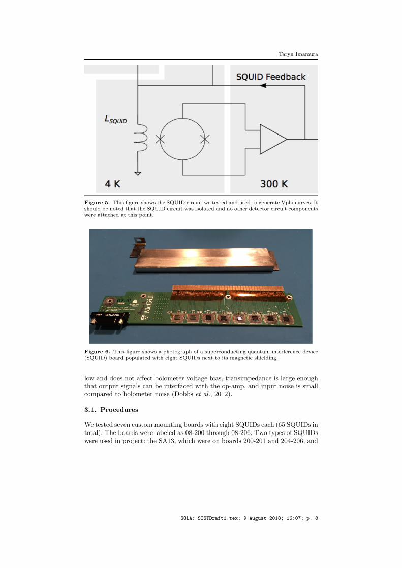
Figure 5. This figure shows the SQUID circuit we tested and used to generate Vphi curves. Itshould be noted that the SQUID circuit was isolated and no other detector circuit componentswere attached at this point.

Figure 6. This figure shows a photograph of a superconducting quantum interference device(SQUID) board populated with eight SQUIDs next to its magnetic shielding.

low and does not affect bolometer voltage bias, transimpedance is large enoughthat output signals can be interfaced with the op-amp, and input noise is smallcompared to bolometer noise (Dobbs et al., 2012).

3.1. Procedures

We tested seven custom mounting boards with eight SQUIDs each (65 SQUIDs intotal). The boards were labeled as 08-200 through 08-206. Two types of SQUIDswere used in project: the SA13, which were on boards 200-201 and 204-206, and



Figure 7. This Figure shows the cryostat setup in which we installed the SQUID Boards(bottom right) for testing.

the StarCryo, which were on boards 202 and 203 with one located on Mezzanine2 Module 4 on board 201. The SA13 SQUIDs have been extensively used inprevious SPT experiments and their behavior is well known. The StarCryoSQUIDs have not been used before and their performance was compared tothe SA13s to supply feedback to their manufacturer. A diagram of the SQUIDcircuit is shown in Figure 5.

First, we used a microscope to read and record each SQUID serial number in aspreadsheet for reference. Next we secured the boards in magnetic shielding. Thismaterial absorbs electromagnetic field lines and would reduce their interferencein SQUID operation. A SQUID board and its magnetic casing is shown in Figure6. Next, we installed the SQUID boards in a cryostat, mounted them on the 2.5K stage of the pulse tube cooler (PTC) as shown in Figure 7, and tuned theSQUIDs so that they operate at their optimum operating point. We used pythonalgorithms entered in terminal to interface with the SQUIDs.

The first step in the tuning process was to heat the SQUIDs using a pythonalgorithm. In this process, current was supplied to a heater resistor next to eachSQUID, raising the devices temperature to its normal state and allowing it tocool quickly. This process reduced the probability of time varying field beingtransformed into spatially trapped flux and was repeated at the beginning ofeach test (Dobbs et al., 2012).

Next, we mapped the SQUID output voltage response and generated “Vphi”curves using a python algorithm that works in the following way. The algorithm


Taryn Imamura

input current biases, Ib, at the Digital-Analog Converter (DAC) though theSQUID’s input coil. The preset parameters did not work for each SQUID sowe changed them to range from 0.6 V to 1.1 V increasing in increments of 0.1V. By convention, the program relays the current bias input in units of Volts.If so desired, the 4.22 KΩ nominal input resistor can be used to convert thisinformation into units of Amps; however, this is not necessary for the purposesof this study. For each current bias Ib, the algorithm steps through values offlux bias, Iif which is the current through the SQUID’s input coil. Finally, the

algorithm measures the voltage out of the op-amp at each Iif , and repeats theprocess.

Figure 8. This figure shows an ideal Vphi curves for the SA13 SQUIDs

We visually checked each Vphi to ensure sure they behaved as expected. Oneof these curves for an SA13 is shown below in Figure 8. This Figure represents anideal Vphi curve because the voltage offset vs flux bias are near perfect sinusoidswhose amplitudes decrease as voltage offset increases. We use the Vphi curvesto extrapolate data such as transimpedance and to choose which current biasoptimizes SQUID performance.

Transimpedance, Z, defines the SQUID small signal response to changes influx bias and it is the quantity that refers the room temperature electronicsnoise back to an equivalent noise current in the SQUID input coil (Dobbs et al.,2012). Simply, transimpedance is a ratio of the output signal to the input sig-nal, or a measurement of the amplifier’s gain. Transimpedance is calculated bytaking the derivative of the Vphi curve. Ideally, we want Z to be maximizedfor optimal SQUID performance. To calculate the optimal transimpedance, weran a python algorithm that tuned the SQUIDs. Generally, any algorithm thattunes the SQUIDs finds the optimal current and flux bias that maximize Z. Theoptimal parameters are those that give a smooth Vphi curve with a high levelof symmetry and steep slope.



Figure 9. This figure shows a non-ideal Vphi curve.

A sinusoidal Vphi curve with the steepest slope represents the ideal currentbias at which to operate the SQUID. For comparison, a non-ideal Vphi curveis shown in Figure 9. This curve is not ideal because its amplitude has a phidependence and its curves are not smooth. In practice, this trait might notalter our data; however, each SQUID amplifies 64 channels and we have a largenumber of SQUIDs available. As a result, we can demand a higher quality ofSQUID performance, even if the reasoning is pedantic.

We then used the Vphi data to extrapolate other behavioral characteristicsof the SQUIDs.

3.2. Analysis and Discussion

We used the Vphi curves and data to calculate three sets of data: transimpedance,peak-to-peak voltage amplitude, and noise. Each data set characterized an im-portant quality in SQUID operation.

After calculating the transimpedance of each SQUID, we generated the his-togram shown in Figure 10 to analyze the overall performance of the system.In Figure 10, the StarCryo data points are shown in green and the SA13 datapoints are shown in purple. As shown in the graph, the StarCryo SQUIDs had alarger spread of transimpedance values and constituted all of the outliers in thedata.

Based on the transimpedance data, several SQUIDs were removed from thefinal circuits and will not be used at the South Pole. The lowest accepted Zthreshold SQUIDs on SPT can have is 400 Ω because SQUIDs tested with atransimpedance below this threshold had too low of a gain and too much noiseresulted in the reading. As seen in Figure 10, four SQUIDs fall below this range


Taryn Imamura

Figure 10. This figure shows a histogram of the transimpedance values for all of the SQUIDs.

and were recorded for removal or further inspection. One SQUID on board 205did not give a transimpedance value most likely due to a broken wirebond ordefective SQUID. This SQUID was also recorded for further inspection.

Next, we calculated the peak-to-peak voltage amplitude, Vpp, of each SQUIDand characterized the data using the histogram shown in Figure 11. This datarepresents the SQUID’s large signal response where distance between the maxand min peaks in each Vphi curve is the current required to produce a fluxquantum through the SQUID coil independent of bias current (Dobbs et al.,2012). We took this measurement as a consistency check for the transimpedancevalues as a SQUID with a high transimpedance (slope) should also yield a largeVpp (distance from peak to trough).

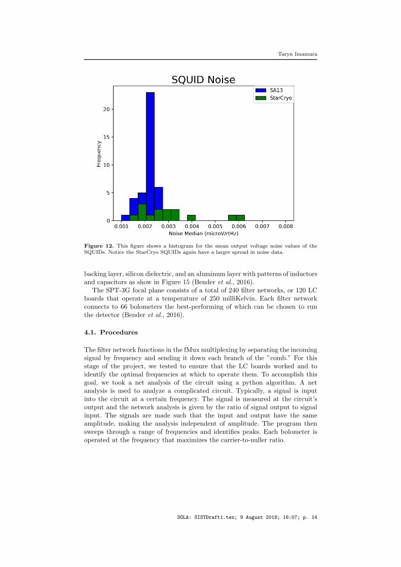
Finally, we measured the SQUID output voltage noise. We collected the noisedata by measuring the output voltage at the op-amp for a few milliseconds at adata rate of 20 MHz. Next, the algorithm measured the Power Spectral Density(PSD). We took the median noise value for each SQUID and graphed them in thehistogram shown in Figure 12. This graph showed the noise of the output voltageof the op-amp. As shown in Figure 12, the StarCryos had a larger spread in theirnoise data and the noise of all SQUIDs centered just above 0.002 µV/rtHz

In addition to the output voltage noise, we computed the input current noise ofthe SQUIDs. Current, voltage, and transimpedance are related by the followingequation:

IZ = V



Figure 11. This figure shows the histogram of the vpp data

We converted the voltage noise data into current noise data by dividing thevoltage noise by the SQUID’s transimpedance. This data was then graphed inFigure 13. This noise data is tighter than the output voltage noise. This isbecause the differing values of Z for each SQUID scale the noise by a differentfactor. By dividing out Z, the noise is scaled by the same factor. As shown inFigure 13, the noise values are around 5 pA/

√Hz. For the detector circuit, the

current noise is expected to be around 15-20 pA/√Hz; however, because the

SQUID circuit was isolated for this portion of testing, the range of noise shownin Figure 13 is acceptable.

Out of 56 SQUIDs, 5 were excluded because they were defective or did notmeet the specifications set for use on SPT-3G. This data yields an 8.9 percentfailure rate with the SQUIDs. Moreover, we found that the StarCryos had alarger distribution in noise and transimpedance data. We will send this feedbackto their manufacturer to help them as they continue to develop their SQUIDtechnology.

4. Testing of Inductor-Capacitor Filter Network

The resonant filter networks, as shown in the circuit diagram in Figure 14. TheLC network of 68 device pairs and wiring is monolithically fabricated on a chip,each of which has three components. These components include an aluminum


Taryn Imamura

Figure 12. This figure shows a histogram for the mean output voltage noise values of theSQUIDs. Notice the StarCryo SQUIDs again have a larger spread in noise data.

backing layer, silicon dielectric, and an aluminum layer with patterns of inductorsand capacitors as show in Figure 15 (Bender et al., 2016).

The SPT-3G focal plane consists of a total of 240 filter networks, or 120 LCboards that operate at a temperature of 250 milliKelvin. Each filter networkconnects to 66 bolometers the best-performing of which can be chosen to runthe detector (Bender et al., 2016).

4.1. Procedures

The filter network functions in the fMux multiplexing by separating the incomingsignal by frequency and sending it down each branch of the ”comb.” For thisstage of the project, we tested to ensure that the LC boards worked and toidentify the optimal frequencies at which to operate them. To accomplish thisgoal, we took a net analysis of the circuit using a python algorithm. A netanalysis is used to analyze a complicated circuit. Typically, a signal is inputinto the circuit at a certain frequency. The signal is measured at the circuit’soutput and the network analysis is given by the ratio of signal output to signalinput. The signals are made such that the input and output have the sameamplitude, making the analysis independent of amplitude. The program thensweeps through a range of frequencies and identifies peaks. Each bolometer isoperated at the frequency that maximizes the carrier-to-nuller ratio.



Figure 13. This figure shows a histogram for the mean current noise values of the SQUIDs.

Figure 14. This figure shows a circuit diagram of the LC resonant filtering network.

Figure 15. This figure shows a photograph of two inductor-capacitor board with cryogenicwiring.


Taryn Imamura

Figure 16. This figure shows the Network Analysis graph of the Carrier-to-Nuller ratiofrequencies.

This particular filter network relies on two input signals, the carrier and thenuller. As a result, we run two network analyses, one for each input signal. Afterrunning a network analysis for each signal, we took the ration of the carrier tonuller signals and generated the graph shown in Figure 16. The circuit usuallyoperates with SQUID feedback as show in Figure 14 which creates a virtualground at that point. Taking the ratio of these input signals simulates theseconditions under which the circuit will operate at the South Pole. Next, thealgorithm identified peaks in the graphs and marked them with a dashed line asshown in Figure 17.

Upon initial visual inspection, we noticed that, in some graphs, the algorithmdid not identify all of the peaks present and, as a result, did not record thesepeaks. This was most likely due to a slight non-uniformity in performance acrossthe LC boards. To ensure the algorithm identified all peaks, we altered itsparameters. We increased the width of the curve the algorithm identifies aspeaks and decreased the signal-to-noise ratio which results in smaller curvesbeing considered peaks.

Finally, we calculated the spacing between individual frequency peaks. Wewant the LC resonant frequencies to be sufficiently far apart to prevent thelikelihood of crosstalk in the data. Crosstalk in the signal would occur if two ormore resonant frequencies were too close that their LC filters registered multiplesignals as having that frequency. The frequency spacing depicted in Figure 18 isideal because it shows that the peaks are separated by at least 20 kHz and thatthe spacing increases as the frequency increases.

5. Conclusions

We found that SQUID transimpedance and noise values were acceptable fordeployment at the South Pole. Ultimately, five SQUIDs did not meet tran-



Figure 17. This figure shows the Carrier to Nuller Network Analysis graph from Figure 16with dotted lines identifying the frequencies of optimized performance.

Figure 18. This figure shows a graph of the frequency spacing of the peaks from Figure 16.

simpedance constraints and were removed from further use. All LC boards passed

our analyses and the ideal frequencies at which to operate them for optimal

detector performance were identified. These components will be transported to

the South Pole during the next Austral Summer for deployment on the SPT.

Additionally, we analyzed the StarCryo SQUID performance compared to

the more developed SA13s. Compared to the SA13s, StarCryos exhibited a

wider range in transimpedance and noise values, making them less precise. This

data will be sent to the StarCryo company as feedback so they can continue to

improve their product and potentially become another source of SQUIDs for the

collaboration.


Taryn Imamura

6. Acknowledgments

Before concluding, I would like to take the time to say thank you to people whohave helped me throughout this summer. First, thank you to my supervisorsBradford Benson, Sasha Rahlin, Adam Anderson, and Donna Kubik for takingthe time to teach me the concepts and skills to complete this project and prepareme for others. Thank you to my mentors: Charlue Orosco, Alex Drlica-Wagner,and Matt Alvarez for helping me prepare my paper and presentation. Thanks toJosemanuel Hernandez for being an incredible friend and person to work with.Finally, I would like to give an enormous thank you to Fermilab and the SISTcommittee for giving me this opportunity and funding my project. This has beenan incredible summer of learning and growth and I and grateful for it.

References

Bender, A., Ade, P., Anderson, A., Avva, J., Ahmed, Z., Arnold, K., Austermann, J., Thakur,R.B., Benson, B., Bleem, L., et al.: 2016, Integrated performance of a frequency domainmultiplexing readout in the spt-3g receiver. In: Millimeter, Submillimeter, and Far-InfraredDetectors and Instrumentation for Astronomy VIII 9914, 99141D. International Societyfor Optics and Photonics. [bender2016]

Benson, B., Ade, P., Ahmed, Z., Allen, S., Arnold, K., Austermann, J., Bender, A., Bleem,L., Carlstrom, J., Chang, C., et al.: 2014, Spt-3g: a next-generation cosmic microwavebackground polarization experiment on the south pole telescope. In: Millimeter, Submil-limeter, and Far-Infrared Detectors and Instrumentation for Astronomy VII 9153, 91531P.International Society for Optics and Photonics. [benson2014]

Carlstrom, J.E., Crawford, T.M., Knox, L.: 2018, Particle physics and the cosmic microwavebackground. arXiv preprint arXiv:1805.06452. [carlstrom2018]

Clarke, J., Braginski, A.I.: 2006, The squid handbook: Applications of squids and squid systems,John Wiley & Sons, ???. [clarke2006]

Dobbs, M., Lueker, M., Aird, K., Bender, A., Benson, B., Bleem, L., Carlstrom, J., Chang,C., Cho, H.-M., Clarke, J., et al.: 2012, Frequency multiplexed superconducting quantuminterference device readout of large bolometer arrays for cosmic microwave backgroundmeasurements. Review of Scientific Instruments 83(7), 073113. [dobbs2012]

Krauss, L.M., Dodelson, S., Meyer, S.: 2010, Primordial gravitational waves and cosmology.Science 328(5981), 989. [krauss2010]


Date post:	20-Oct-2021
Category:	Documents
Upload:	others
View:	1 times
Download:	0 times

Analysis and Characterization of SPT-3G Multiplexing ...

Documents