Analysis of a Load Step Test at Ringhals 4 NPP using...

Analysis of a Load Step Test atRinghals 4 NPP using RELAP5 CodeModel Validation and Verification

Master’s Thesis in Nuclear Science and Technology

ATHANASIOS STATHIS

Department of Applied PhysicsCHALMERS UNIVERSITY OF TECHNOLOGYGothenburg, Sweden 2015

Master’s thesis 2015:NN

Analysis of a Load Step Test at Ringhals 4NPP Using RELAP5 Code

Model Validation and Verification

ATHANASIOS STATHIS

Department of Applied PhysicsDivision of Nuclear Engineering

Chalmers University of TechnologyGothenburg, Sweden 2015

Analysis of a Load Step Test at Ringhals 4 NPP using RELAP5 Code.Model Validation and Verification.ATHANASIOS STATHIS

© ATHANASIOS STATHIS, 2015.

Supervisor: Dr. Jozsef Bánáti, Department of Applied PhysicsExaminer: Assoc. Prof. Anders Nordlund, Department of Applied Physics

Master’s Thesis 2015:NNDepartment of Applied PhysicsDivision of Nuclear EngineeringChalmers University of TechnologySE-412 96 GothenburgTelephone +46 31 772 1000

Cover: 3-loop Westinghouse Pressurised Water Reactor [5].

Typeset in LATEXPrinted by [Name of printing company]Gothenburg, Sweden 2015

iv

Analysis of a Load Step Test at Ringhals 4 NPP Using RELAP5 Code.Model Validation and Verification.ATHANASIOS STATHISDepartment of Applied PhysicsChalmers University of Technology

AbstractRinghals 4 unit, a Westinghouse deign Pressurized Water Reactor, has recentlyundergone a pressurizer and steam generator replacement. In March 2015 the reactorwas licenced to operate at the uprated 3300 MWth nominal thermal power level.Load Step Test is among the first tests performed in the reactor at the upratedpower conditions.

During the Load Step Test, while the reactor is in steady state, the turbinepower is sharply reduced by 10 %. Fast insertion of the control rods follows and thereactor is stabilized in an intermediate steady state. After 3000 s in the intermediatesteady state the control rods are quickly withdrawn in order to sharply increase theturbine power by 10 % and restore the reactor to its nominal steady state.

The purpose of the Load Step Test is to verify that the control systems canmitigate the transient. The data from this test can be used for the assessmentand improvement of RELAP5 model of Ringhals 4. Validation of the model wasperformed by the simulation of the transient.

Thus, the first step is that the code reaches a realistic steady state close to theone of the plant in the beginning of the test. This task is accomplished. The chal-lenges occurred during this stage are mentioned as well the way they were tackled.In addition, strategies for achieving steady state are touched upon.

The next step is the simulation of the whole transient. The process/way ofthinking that led to specific improvements in the model is described, as well as thekey parameters for the further improvement of the model.

In the end, the "goodness" of the improved model is assessed using the FastFourier Transformed Method (FFTBM). FFTBM proves that the model is capableof predicting the transient quite accurately.

Keywords: Fast Fourier Transform Based Method (FFTBM), Load Step Test,RELAP5, Ringhals 4, Transient.

v

AcknowledgementsI would like to express my deep gratitude to my beloved parents, Kaloudis andIrini, and to my beloved brother Vasilis. Thank you for supporting me during mymaster studies despite the financial confinements imposed by the Greek financialcrisis. Thank you very much for your trust and your encouragement. I wouldn’tmake it without you. I devote this thesis to you. I send you my love and my bestwishes to each one to you personally.

I would also like to thank my supervisor, Dr. Jozsef Bánáti for his vital supportand help during this thesis project. I am very glad to cooperate with such anexceptional man. As a supervisor he was very inspiring and kindly offered me thechance to become co-author in one his scientific reports. I have benefited a lot fromhis engineering thinking. I appreciate him a lot and I will definitely miss the nicediscussions we had during our sessions.

Moreover, I would like to thank my industry counsellor, Marie Hagman, for herkind support and her encouragement as well as for her valuable advices.

I also feel thankful for Dr. Andrej Prošek for his valuable contribution to mymaster thesis project. Dr. Prošek kindly answered my questions about FFTBM,providing the programme being used for the FFTBM calculations as well as papersand publications about FFTBM issues.

Special thanks my opponents, Karin Warholm and Roger Hurtig for their com-ments, as well as my examiner Dr. Anders Nordlund for supporting my participationin RELAP5 meetings along with my supervisor.

And last but not least, I would like to send my warm regards to Dr. NikosPetropoulos from Athens. He is the man who taught me the first course in NuclearEngineering and who inspired me to follow this discipline.

Athanasios Stathis, Gothenburg, November 2015

vii

Contents

List of Figures xi

List of Tables xv

Abbreviations xvii

1 Introduction 11.1 Nuclear Energy in Sweden . . . . . . . . . . . . . . . . . . . . . . . . 21.2 Description of LWRs . . . . . . . . . . . . . . . . . . . . . . . . . . . 31.3 Pressurized Water Reactor (PWR) . . . . . . . . . . . . . . . . . . . 4

1.3.1 The Pressurizer (PRZ) . . . . . . . . . . . . . . . . . . . . . . 51.3.2 The Steam Generator . . . . . . . . . . . . . . . . . . . . . . . 6

1.4 Ringhals 4 unit . . . . . . . . . . . . . . . . . . . . . . . . . . . . . . 81.4.1 The new SG . . . . . . . . . . . . . . . . . . . . . . . . . . . . 8

1.5 Aim of the thesis project . . . . . . . . . . . . . . . . . . . . . . . . . 101.6 Thesis outline . . . . . . . . . . . . . . . . . . . . . . . . . . . . . . . 10

2 Modelling of Ringhals 4 Unit 112.1 Modelling of Primary Side . . . . . . . . . . . . . . . . . . . . . . . . 11

2.1.1 Modelling of Reactor Pressure Vessel . . . . . . . . . . . . . . 122.1.2 Heat Source . . . . . . . . . . . . . . . . . . . . . . . . . . . . 132.1.3 Modelling of PRZ . . . . . . . . . . . . . . . . . . . . . . . . . 13

2.2 Modelling of Secondary Side . . . . . . . . . . . . . . . . . . . . . . . 142.2.1 Modelling of Steam Generators . . . . . . . . . . . . . . . . . 14

2.2.1.1 Nodalization of SGs Primary Side . . . . . . . . . . . 142.2.1.2 Nodalization of SGs Secondary Side . . . . . . . . . 14

2.2.2 Turbine Modelling . . . . . . . . . . . . . . . . . . . . . . . . 152.2.3 Inflow Boundary Condition . . . . . . . . . . . . . . . . . . . 15

3 The Load Step Test 21

4 Load Step Test Analysis (1) - Calculating Steady-State 294.1 Achieving Steady-State . . . . . . . . . . . . . . . . . . . . . . . . . . 29

4.1.1 Strategies to reach Steady-State . . . . . . . . . . . . . . . . . 314.2 Steady-State Results . . . . . . . . . . . . . . . . . . . . . . . . . . . 31

5 Load Step Test Analysis (2) - Transient Analysis 41

ix

Contents

5.1 Thermal Power Ratio . . . . . . . . . . . . . . . . . . . . . . . . . . . 415.2 Discrepancies in the PRZ . . . . . . . . . . . . . . . . . . . . . . . . . 445.3 Transient Analysis Results . . . . . . . . . . . . . . . . . . . . . . . . 475.4 Transient Analysis Concluding Remarks . . . . . . . . . . . . . . . . 54

6 Accuracy Quantification using Fast Fourier Transform Based Method(FFTBM) 576.1 FFTBM Outline . . . . . . . . . . . . . . . . . . . . . . . . . . . . . 57

6.1.1 Average Amplitude . . . . . . . . . . . . . . . . . . . . . . . . 576.1.2 Additional Measures for Accuracy Quantification . . . . . . . 59

6.2 Methodology for Code Accuracy Quantification . . . . . . . . . . . . 606.3 FFTBM Analysis . . . . . . . . . . . . . . . . . . . . . . . . . . . . . 606.4 FFTBM Results . . . . . . . . . . . . . . . . . . . . . . . . . . . . . . 616.5 FFTBM Analysis Concluding Remarks . . . . . . . . . . . . . . . . . 69

7 Conclusion 717.1 Summary - Main Conclusions . . . . . . . . . . . . . . . . . . . . . . 717.2 Proposals for Future Work . . . . . . . . . . . . . . . . . . . . . . . . 71

Bibliography 73

x

List of Figures

1.1 Nuclear reactors of Sweden [30]. . . . . . . . . . . . . . . . . . . . . . 21.2 Timeline of nuclear reactors of Sweden [32]. . . . . . . . . . . . . . . 31.3 PWR outline [31]. . . . . . . . . . . . . . . . . . . . . . . . . . . . . . 41.4 A Pressurizer (PRZ) [5]. . . . . . . . . . . . . . . . . . . . . . . . . . 61.5 A Westinghouse Steam Generator [29]. . . . . . . . . . . . . . . . . . 71.6 Timeline of Ringhals 4 unit [4]. . . . . . . . . . . . . . . . . . . . . . 81.7 New SG of Ringhals 4 [5]. . . . . . . . . . . . . . . . . . . . . . . . . 9

2.1 Radial discretization of the core of Ringhals 4 unit with 157 fuelassemblies[5, 7]. . . . . . . . . . . . . . . . . . . . . . . . . . . . . . . 12

2.2 Nodalization of the PRZ [5]. . . . . . . . . . . . . . . . . . . . . . . . 132.3 Nodalization scheme of the primary side of Ringhals 4 unit [5, 7]. . . 162.4 Nodalization of the core. [5, 7]. . . . . . . . . . . . . . . . . . . . . . 172.5 Secondary side discretization of Ringhals 4 unit [5, 7]. . . . . . . . . . 182.6 Nodalization of the SG. [5, 7]. . . . . . . . . . . . . . . . . . . . . . . 19

3.1 Neutron flux and control rod position. . . . . . . . . . . . . . . . . . 223.2 Pressure in the PRZ with time measured by three different channels. 233.3 Level in the PRZ measured by three different channels. . . . . . . . . 233.4 Pressure in the steam lines as measured by the first channel of each

steam line. . . . . . . . . . . . . . . . . . . . . . . . . . . . . . . . . . 243.5 Level in SGs as measured by the first channel of each SG. . . . . . . . 243.6 Temperature in the hot legs as measured by the first channel of each

hot leg. . . . . . . . . . . . . . . . . . . . . . . . . . . . . . . . . . . . 253.7 Temperature in the cold legs as measured by the first channel of each

cold leg. . . . . . . . . . . . . . . . . . . . . . . . . . . . . . . . . . . 253.8 Flow-rate in the three loops as measured by the first channel of each

loop. . . . . . . . . . . . . . . . . . . . . . . . . . . . . . . . . . . . . 263.9 Feedwater-flow rate in the three loops measured by three different

channels. . . . . . . . . . . . . . . . . . . . . . . . . . . . . . . . . . . 263.10 Steam-flow rate in the three steam lines as measured by the first

channel of each steam line. . . . . . . . . . . . . . . . . . . . . . . . . 273.11 Spraying flow controllers output signals (red and green lines) and pro-

portional heaters controller output signals (blue and magenta lines),each measured by two channels. . . . . . . . . . . . . . . . . . . . . . 27

4.1 Thermal Power. . . . . . . . . . . . . . . . . . . . . . . . . . . . . . . 32

xi

List of Figures

4.2 Loop flow-rate. . . . . . . . . . . . . . . . . . . . . . . . . . . . . . . 334.3 Pressure in SGs. . . . . . . . . . . . . . . . . . . . . . . . . . . . . . . 334.4 Level steady-state value in the SGs. . . . . . . . . . . . . . . . . . . . 344.5 Pressure in the PRZ. . . . . . . . . . . . . . . . . . . . . . . . . . . . 344.6 Level in the PRZ. . . . . . . . . . . . . . . . . . . . . . . . . . . . . . 354.7 Feedwater flow-rate. . . . . . . . . . . . . . . . . . . . . . . . . . . . 354.8 Feedwater temperature. . . . . . . . . . . . . . . . . . . . . . . . . . 364.9 Temperature in hot leg. . . . . . . . . . . . . . . . . . . . . . . . . . . 364.10 Temperature in cold leg. . . . . . . . . . . . . . . . . . . . . . . . . . 374.11 Average temperature for the three loops in the hot leg. . . . . . . . . 374.12 Steam temperature. . . . . . . . . . . . . . . . . . . . . . . . . . . . . 384.13 Steam pressure. . . . . . . . . . . . . . . . . . . . . . . . . . . . . . . 38

5.1 Steam flow-rate and thermal power ratio used in the calculation. Thethermal power ratio is deduced from the neutron flux test data. . . . 43

5.2 Steam flow-rate (left axis) and thermal power ratio used in the cal-culation. The thermal power ratio is calculated using the feedwaterflow-rate and the enthalpies of the feedwater and of the steam. . . . . 43

5.3 Steam flow-rate (left axis) and thermal power ratio used in the calcu-lation. The thermal power ratio is calculated based on the tempera-ture difference between the hot and the cold leg. . . . . . . . . . . . . 44

5.4 Charging flow-rate in the primary side. Discrepancies occur duringthe whole transient, however they intensify during the sharp thermalpower decrease and increase. . . . . . . . . . . . . . . . . . . . . . . . 45

5.5 Pressure in the PRZ. Noticeable discrepancies occur between 500 and1500 s as well as after 4000 s. . . . . . . . . . . . . . . . . . . . . . . 46

5.6 Water level in the PRZ. Noticeable discrepancies after 500 s. . . . . . 465.7 Output of spraying flow-rate controller. This control signal is trans-

lated into spraying flow-rate through the valve characteristic curve. . 475.8 Thermal Power input for the transient runs. . . . . . . . . . . . . . . 485.9 Pressure in the pressurizer. . . . . . . . . . . . . . . . . . . . . . . . . 485.10 Level in the PRZ. . . . . . . . . . . . . . . . . . . . . . . . . . . . . . 495.11 Pressure in the SG. . . . . . . . . . . . . . . . . . . . . . . . . . . . . 495.12 Level in the SG. . . . . . . . . . . . . . . . . . . . . . . . . . . . . . . 505.13 Temperature in hot leg. . . . . . . . . . . . . . . . . . . . . . . . . . . 505.14 Temperature in cold leg. . . . . . . . . . . . . . . . . . . . . . . . . . 515.15 Loop average temperature. . . . . . . . . . . . . . . . . . . . . . . . . 515.16 Feedwater flow-rate in the secondary side. . . . . . . . . . . . . . . . 525.17 Steam flow-rate. . . . . . . . . . . . . . . . . . . . . . . . . . . . . . . 525.18 Charging flow-rate (given as boundary condition). . . . . . . . . . . 535.19 Proportional heaters capacity. . . . . . . . . . . . . . . . . . . . . . 535.20 Spraying flow-rate signal. . . . . . . . . . . . . . . . . . . . . . . . . 54

6.1 Average amplitude of the primary pressure. . . . . . . . . . . . . . . . 636.2 Average amplitude of level in the PRZ. . . . . . . . . . . . . . . . . . 636.3 Average amplitudes of the pressure in the SGs. . . . . . . . . . . . . . 646.4 Average amplitudes of the levels in the SGs. . . . . . . . . . . . . . . 64

xii

List of Figures

6.5 Average amplitudes of the hot leg temperatures in the SGs. . . . . . . 656.6 Average amplitudes of the cold leg temperatures in the SGs. . . . . . 656.7 Average amplitudes of the average loop temperatures. . . . . . . . . . 666.8 Average amplitudes of the feedwater flow-rates in the SGs. . . . . . . 666.9 Average amplitudes of the steam flow-rates in the SGs. . . . . . . . . 676.10 Average amplitude of the proportional heaters capacity. . . . . . . . . 676.11 Average amplitude of the spraying flow-rate signal. . . . . . . . . . . 686.12 Total average amplitude. . . . . . . . . . . . . . . . . . . . . . . . . . 68

xiii

List of Figures

xiv

List of Tables

1.1 Data about the nuclear reactors in Sweden. . . . . . . . . . . . . . . . 3

4.1 Steady-state values achieved and expected/desired values accordingto the test data. . . . . . . . . . . . . . . . . . . . . . . . . . . . . . . 32

6.1 Weighting factors for different measured quantities (SB-LOCA) [8,12, 22]. . . . . . . . . . . . . . . . . . . . . . . . . . . . . . . . . . . . 59

6.2 FFTBM analysis variables, weighting factors and results for the 0 −4500 s interval . . . . . . . . . . . . . . . . . . . . . . . . . . . . . . . 62

xv

List of Tables

xvi

Abbreviations

AA Average AmplitudeAAtot Total Average AmplitudeBE Best Estimate

BWR Boiling Water ReactorCV CS Chemical and Volume Control SystemDFT Discrete Fourier TransformationFFT Fast Fourier Transformation

FFTBM Fast Fourier Transform Based MethodLOCA Loss of Coolant AccidentLWR Light Water ReactorMCP Main Circulation PumpND Number of Discrepancies

PHWR Pressurized Heavy Water ReactorPORV Power Operated Relief ValvePRZ PressurizerPWR Pressurized Water ReactorRHRS Residual Heat Removal SystemRPV Reactor Pressure Vessel

SB − LOCA Small Break Loss of Coolant AccidentSCRAM Safety Control Rods Activator Mechanism

SG Steam GeneratorV A Variable Accuracy

V Amax Maximum Variable AccuracyV Amin Minimum Variable Accuracy

xvii

List of Tables

xviii

1Introduction

Nuclear Power is a source of energy used as base load with minimum CO2 emissions.The power density of a nuclear power plant produces by far more power than theconventional and renewable power sources (e.g. wind mills farms, solar panels farm).Nuclear power is also considered cheap as the lifetime of an ordinary plant can beextended to operate around 60 years and the basis. The fuel, uranium, is cheap andits price does not fluctuate significantly.

Uranium price is very unlikely to vary significantly due to political reasons. Itis worth mentioning that the fuel used in most of the light water reactors (LWRs)is enriched around 3-3.5 % 235U . 235U is the isotope that contributes to the energyoutput of the fuel. Thus, there is a huge margin of improvement in fuel efficiency.

Despite the above favorable characteristics of nuclear power public opinion inmany countries is very sceptic about its adoption, mainly due to safety concerns.Chernobyl and Fukushima accidents have damaged a lot the reputation of nuclearenergy.

However the safety of the current third generation reactors has massively im-proved the last decades and nuclear energy is considered a safe energy source. Ahuge effort has been put on the mitigation and prediction/simulation of the most im-portant class of accidents, the loss of coolant accidents (LOCAs) using small scaledfacilities of commercial prototype reactors. In addition, tests are performed in thereactors themselves in order to verify the ability of the control systems to mitigatedeviations from ordinary operation conditions. Among those maneuverability tests,the Load Rejection [6], SCRAM Test and the Load Step Test [7, 4] are the mostimportant. The complexity and the time required for its analysis make the LoadStep Test very suitable for a master thesis project. This master thesis deals withthe analysis of the Load Step Test performed in 2015-03-03 in Ringhals 4 unit.

1

1. Introduction

1.1 Nuclear Energy in SwedenNuclear energy in Sweden accounts for 41.47 % of the total electricity productionin the country just behind hydro-power electricity production which accounts foraround 45 % of the total electricity production.

Figure 1.1: Nuclear reactors of Sweden [30].

The first reactor to be critical in Sweden was a Pressurized Heavy Water Reactor(PHWR) in Ågesta in 1964. This reactor had a power output of 10 MWe and wasused mainly for district heating of the wider Stockholm region. However, it produceda small amount of electricity also. Ågesta reactor operated for 10 years, until 1974when it was permanently shut down.

The first commercial reactor commissioned was Oskarshamn 1 Boiling WaterReactor (BWR) in 1972. Until 1980 another 9 units were commissioned in the sitesof Oskarshamn, Ringhals, Forsmark and Barsebäck.

In the aftermath of Three-Mile-Island accident a referendum was held in Swedenconcerning the future of nuclear energy in the country. The outcome of the referen-dum was to continue with the construction of Ringhals 3 and 4 units and that thereactor of operating units would be 12. In addition the safety systems of Barsebäck3 unit had to be improved. It was also decided that all the units should be phasedout until 2010.

With the occurrence Chernobyl accident in 1985, a new legislation had beenratified in 1987 by the parliament which prohibited the construction of new units.However, in a poll held in 2001 the Swedish people seemed to have a very positiveattitude towards nuclear. 76 % voted for the continuation of nuclear industry.

In 2010 the legislation was modified to allow for improvements in the operatingunits. Life extension for most of the units was granted and investments were headedtowards improving the operated units.

Finally, in 2014 the government has ceased any initiatives for building new unitsand the country is heading towards to the complete phase out of its nuclear powerplants in the foreseeable future.

2

1. Introduction

During 2015 Oskarshamn 2 unit phased out and Oskarshamn 1 unit along withRinghals units 1 and 2 are also expected to stop electricity production by 2020.Barsebäck units 1 and 2 were phased out in 1999 and 2005 respectively.

Reactor Unit Type Status Operator Gross Capacity (MWe) Commercial Operation Decommissioning

Forshmark-1 BWR Operational Vattenfall 1022 1980 2040Forshmark-2 BWR Operational Vattenfall 1158 1981 2041Forshmark-3 BWR Operational Vattenfall 1212 1985 2045Oskarshamn-1 BWR Operational OKG 492 1972 2017-19Oskarshamn-2 BWR Operational OKG 661 1974 2015Oskarshamn-3 BWR Operational OKG 1450 1985 2035 or 2045Ringhals-1 BWR Operational Vattenfall 910 1976 2020Ringhals-2 PWR Operational Vattenfall 847 1975 2019Ringhals-3 PWR Operational Vattenfall 1117 1981 2041Ringhals-4 PWR Operational Vattenfall 1168 1983 2043Ågesta PHWR Shutdown Barsebäck Kraft AB 12 1964 1974Barsebäck-1 BWR Shutdown Barsebäck Kraft AB 615 1975 1999Barsebäck-2 BWR Shutdown Barsebäck Kraft AB 615 1977 2005

Table 1.1: Data about the nuclear reactors in Sweden.

Figure 1.2: Timeline of nuclear reactors of Sweden [32].

1.2 Description of LWRsLight Water Reactors (LWRs) are reactors that use water both as moderator andcoolant. Two designs for LWRs exist. The Pressurized Water Reactor (PWR) andthe Boiling Water Reactor (BWR). These types of reactors use Uranium as nuclearfuel usually 3 % enriched in U235 (the rest comprises of 238U atoms). Thermal energycomes primarily from the fission of 235U .

3

1. Introduction

A fission reaction of 235U occurs when a slowed down neutron/thermal neutronis absorbed by an 235U nucleus. This reaction yields two or three fast neutronsalong with two medium-heavy nuclei and the release of 200MeV energy. These fastneutrons need to be slowed down/moderated so as to be absorbed by other 235Unuclei. Fast neutrons loose most of their kinetic energy by colliding with watermolecules (water used as moderator).

Successive fissioning of 235U leads in a chain reaction and increasing energy outputwhich is controlled by the use of neutron absorbers. In PWRs diluted boron inwater and control rods entering from the bottom of the reactor are used as neutronabsorbers.

Thermal energy is also produced by fissioning of 238U by fast neutrons and byfissioning of 236U and 239Pu. The two last isotopes are formatted by some of thesuccessive decays of 238U when it absorbs fast neutrons.

The fission energy produced is removed by turbulent water passing through chan-nels in the fuel rods to be further utilised for electricity production and for coolingthe fuel rods (water used as coolant).

1.3 Pressurized Water Reactor (PWR)A PWR consist of two circuits, the primary and the secondary. The primary circuitincludes the core the pressurizer (PRZ) and the primary side of the steam generator(SG) and the main circulation pumps (MCP). The secondary circuit includes thesecondary side of the SG as well as the turbines and the condenser.

Figure 1.3: PWR outline [31].

4

1. Introduction

The SG acts as heat exchanger between the primary and the secondary circuitswhereas the PRZ is used for the regulation of the primary pressure.

Energy produced by fission reactions in the core heats the water in the primaryside. The heated water passes from the SG where heat exchange occurs with therelatively cooler water of the secondary side of the SG. Hence, the heated watercools down and recirculates in the primary circuit.

The water in the cold side of the SG receives the heat of the water in the primarycircuit and steam is produced. The steam is headed to the high and low pressureturbines and electricity is produced. After the passage from the turbines, condensersare used to condense the steam which is then recirculated in the secondary circuit.

A brief description of the PRZ and of a SG takes place in the following subsec-tions.

1.3.1 The Pressurizer (PRZ)The PRZ (figure 1.4) is a tank which contains water in its lower part and steamin the upper part, and is used to regulate the pressure in the primary circuit. Inthe upper part the PRZ is connected to a power operated relief valve (PORV) anda spray nozzle, whereas in the bottom part it is equiped with proportional andON-OFF heaters.

The purpose of the PORV and of the spray nozzle is to relieve the pressureincrease in the primary side. PORV achieves that by letting steam to be blowndown through it. The spray nozzle achieves pressure relief by spraying water whichcondenses an amount of steam. Yet, there is always a constant small amount ofspraying in steady state conditions in order to minimize the probability of theirblockage in case of a transient condition.

On the other hand ON-OFF and proportional heaters (both pressure actuated)are used to increase the pressure. Both kind of heaters increase the pressure in thePRZ by expanding the water through heating. Proportional heaters are actuatedin case of large pressure drops and they function always at full capacity. They areused to compensate smaller pressure drops and their capacity is analogous with thepressure deviation from the nominal value.

5

1. Introduction

Figure 1.4: A Pressurizer (PRZ) [5].

1.3.2 The Steam Generator

The SG (figure 1.5) is a tank filled with water which is penetrated by primary sidetubes of U-shape. Water of the SG in the vicinity of U-tubes lies at smaller pressureand temperature than the water flowing through them. As a result heat transferoccurs and the water around the U-tubes starts boiling. This lower section of the SGwhere boiling occurs is referred to as evaporation section. The wet steam producedin the evaporator passes in the steam drum section where wet steam is dried insteam separators before it is headed in the turbines.

6

1. Introduction

Figure 1.5: A Westinghouse Steam Generator [29].

7

1. Introduction

1.4 Ringhals 4 unitRinghals 4 unit is a 3-loop Westinghouse design pressurized water reactor (PWR).Ringhals 4 was commissioned in 1982 with 2783 MWth nominal power level. In2011 the original Westinghouse PRZ and SGs were replaced with AREVA-designcomponents and the turbines were modernized. As a result the reactor would havethe potential to operate for 3300 MWth. In the same year, the first start-up testswere performed with the new components in place, yet, the reactor was still licencedto operate at 2783 MWth nominal power level. After three years of test operationnew test were performed in March 2015 and the reactor was licensed to operate at3300 MWth nominal power level. The Load Step Test was among the tests performedin 2011 and 2015.

Figure 1.6: Timeline of Ringhals 4 unit [4].

1.4.1 The new SGThe new SG is more efficient than the old one due to its innovative design. The newfeatures of the SG are the divider plate and the double wrapper which covers half ofthe bundle wrapper perimeter (figure 1.7). It is known from thermodynamics thatthe heat transfer in the SG depend on the temperature difference between the hotand the cold leg. Increasing the temperature difference translates to an increase inextracted heat from the fluid.

Hence, the droplets coming from the steam separator recirculates in the outerdowncomer. 90 % in the hot side where the droplets are mixed in the bottom of theSG with the fluid in the hot leg, and 10 % in the cold side. As a result, the fluid

8

1. Introduction

temperature in the hot side increases.At the same time feedwater is injected in the downcomer surrounding half of the

bundle wrapper perimeter. The feedwater is mixed with the 10% of the recirculateddroplets in the bottom of the cold side of the SG, and then both are mixed with thefluid flowing in the cold leg. Thus, the temperature of fluid in the cold side drops.

The divider plate separates the cold from the hot side of the SG so that thistemperature difference is sustained. Consequently, more heat is extracted.

Figure 1.7: New SG of Ringhals 4 [5].

9

1. Introduction

1.5 Aim of the thesis projectIn general the aim of the present thesis project is the evaluation and assessment ofthe RELAP5 model of Ringhals 4 unit being used. More specifically, the calculatedresults are compared to measured plant data. The goal is to modify/improve themodel and increase its predicting capabilities for reproduction of the calculated dataas accurately as possible.

The ultimate goal is to obtain a RELAP5 model that will be capable of predictingevery possible transient.

A new contribution of this master thesis is the assessment of the updated modelusing the FFTBM with signal mirroring. It is the first time in Sweden that thismethod is applied for the code assessment of a real plant start-up and maneuver-ability test.

1.6 Thesis outlineThis thesis is divided in six chapters. Chapter 1 is a brief introduction in nuclearenergy. It describes the principles of nuclear power production, the PressurizedWater Reactor (PWR) and the time-line of nuclear industry in Sweden.

Chapter 2 refers to RELAP5 model of Ringhals 4 unit. The most importantparameters and features of the model are described, whereas chapter 3 is devotedto the Load Step performed at 2015-03-03. The reasons for the performance of thiskind of experiment are mentioned and the experimental results are presented.

In order to run the whole transient it is essential for the code to achieve a cal-culated steady-state close to the real one, as indicated by the plant data. Hence,Chapter 4 is devoted to steady-state. The method used for achieving steady-stateis explained and the calculated steady-state results are presented.

Chapter 5 deals with the analysis of the whole transient and the correspondingresults are presented. Issues raised during the transient runs are described as wellas the way they were mitigated. In the end of the chapter the most importantoutcomes of the transient analysis are summarized.

Chapter 6 is dedicated to Fast Fourier Transform Based Method (FFTBM) withsignal mirroring. The outline of FFTBM is described as well as the results and theconclusions of code assessment quantification.For the FFTBM analysis, JSI FFTBMAdd-in 2007 was used, an Excel 2007 application implemented by Dr. Andrej Prošekfrom Jožef Stefan Institute in Ljubljana.

Finally, chapter 7 presents an outline of the outcomes of this thesis, and elaborateson topics raised during steady-state and transient runs. Proposals for future projectsare also included.

10

2Modelling of Ringhals 4 Unit

The purpose of this chapter is to give some general information about the RELAP5model of Ringhals 4. For the scope of this thesis RELAP5/MOD3.3 is used, whichis the newest version of RELAP5 for the time being.

RELAP5 is a best estimate code used for the simulation of transients and pos-tulated accidents. It is a generic code which can also be used for the simulation ofother than nuclear thermal systems. It also plays an important role in licencing,evaluation of mitigation strategies and operational guidelines [5, 7].

Version RELAP5/MOD3.3 is based on a non-homogeneous non-equilibrium modelfor the two phase system which is solved using a partial numerical scheme [11]. Itsimulates important first-order effects related with transients in a simple manner sothat the computational cost remains sufficiently low.

RELAP5 model of Ringhals 4 is a "stand alone" thermohydraulic model compris-ing of two main parts, the primary and the secondary side. It is a representation ofthe prototype reactor and as such it is the compromise between geometrical fidelity,results accuracy, complexity and cpu time. Inevitably, a number of simplificationsare adopted as will be described in the remainder of the chapter.

2.1 Modelling of Primary SideThe most important major components included in the nodalization of the primaryside in figure 2.3 are:

• The reactor pressure vessel (RPV).• The pressurizer (PRZ).• The safety and relief valves.• The normal letdown.• The main circulation pumps (MCPs).• The residual heat removal system (RHRS).• The charging system.A description of the modelling of the most related major components follows in

the upcoming subsections.

11

2. Modelling of Ringhals 4 Unit

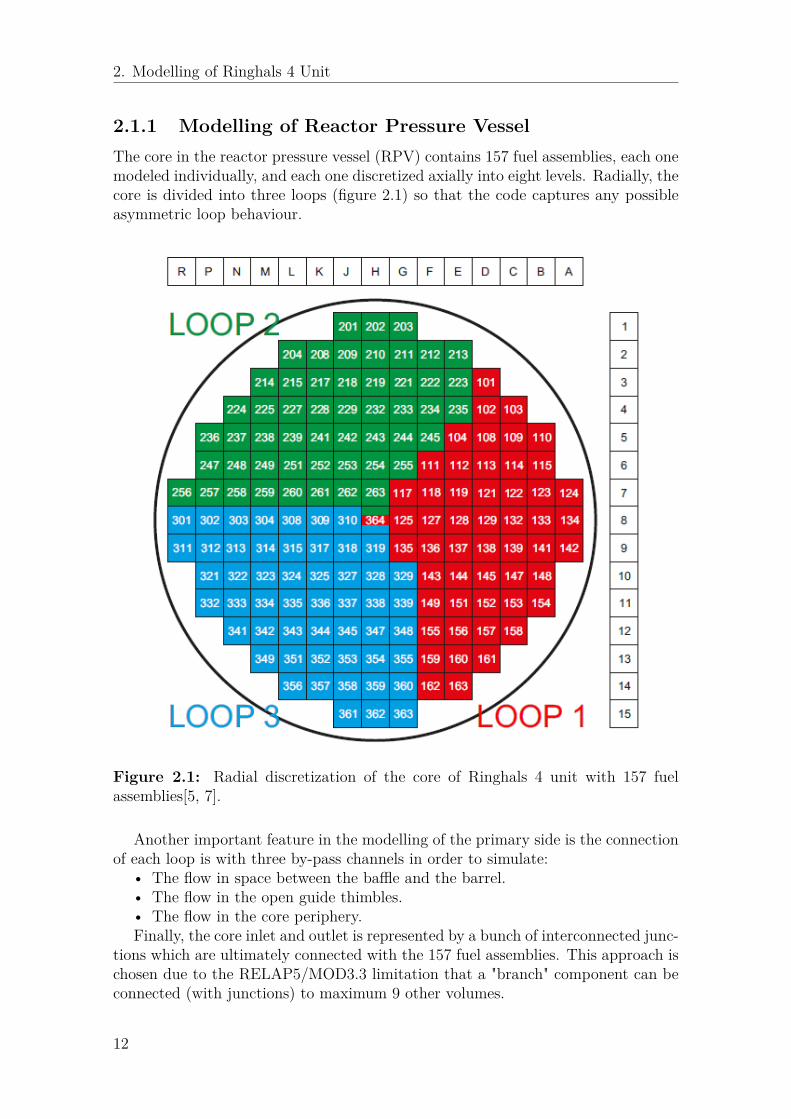
2.1.1 Modelling of Reactor Pressure VesselThe core in the reactor pressure vessel (RPV) contains 157 fuel assemblies, each onemodeled individually, and each one discretized axially into eight levels. Radially, thecore is divided into three loops (figure 2.1) so that the code captures any possibleasymmetric loop behaviour.

Figure 2.1: Radial discretization of the core of Ringhals 4 unit with 157 fuelassemblies[5, 7].

Another important feature in the modelling of the primary side is the connectionof each loop is with three by-pass channels in order to simulate:

• The flow in space between the baffle and the barrel.• The flow in the open guide thimbles.• The flow in the core periphery.Finally, the core inlet and outlet is represented by a bunch of interconnected junc-

tions which are ultimately connected with the 157 fuel assemblies. This approach ischosen due to the RELAP5/MOD3.3 limitation that a "branch" component can beconnected (with junctions) to maximum 9 other volumes.

12


2.1.2 Heat Source

So far, RELAP5 model of Ringhals 4 unit is not coupled with a neutronic code. As aresult this model accounts only for the thermohydraulic features of Ringhals 4 unit,since the reactivity feedbacks and small variations in power cannot be accountedfor. Thus, the thermal power is given as function of time (in a table form). Thermalpower strongly affects a number of variables such as the primary pressure, fluidtemperatures etc.

2.1.3 Modelling of PRZ

The PRZ is modelled as a pipe with 12 components (figure 2.2). The first twovolumes in the bottom of the PRZ contain the proportional heaters and the ON-OFF heaters.

Figure 2.2: Nodalization of the PRZ [5].

13


Proportional heaters regulate moderate pressure deviations and their output isproportional to the pressure deviation from the nominal value, as their name indi-cates. Their maximum output is 375 kW . ON-OFF heaters operate at 1125 kWpower output and they are actuated in case of larger pressure deviations.

The top volume of the PRZ is connected with the modelled spray nozzle (modelledas valve component) and the modelled power operated relief valve (PORV). In thereal plant two spraying valves exist, each injecting maximum 14.52 kg/s, which areconnected to cold legs of loop-1 and 2. In the current R4 RELAP5 model these twospraying valves are modelled as one, which is connected to the cold leg of loop-2,having 28.040 kg/s maximum flow rate.

2.2 Modelling of Secondary SideAs far as the secondary side concerned, the nodalization scheme presented in figure2.5 includes the following major parts:

• The three hot legs (HLs) and cold legs (CLs).• The three steam generators (SGs).• The feedwater system.• The steam dumping lines.• The turbines.As it is mentioned above, a number of simplifications take place in the model.

For instance, the turbine and the condensers in the secondary side are not modelled.In such cases it is quite regular to use boundary conditions.

2.2.1 Modelling of Steam GeneratorsThe nodalization scheme of a SG is presented in figure 2.6. Particularly, this is thenodalizaton scheme of SG-1, but the other two steam generators have exactly thesame nodalization. The only difference lies in the first digit in the numbers assignedto each volume component. For instance, the inlet plenum in SG-1 is denoted ascontrol volume 120 whereas in SG-2 as control volume 220.

2.2.1.1 Nodalization of SGs Primary Side

Water enters in the inlet plenum, volume 120, which is modelled as branch com-ponent, it flows along the U-tubes and exits from the outlet plenum, volume 140,which is modelled as branch component as well. U-tubes, volumes 130-01 to 130-22,are modelled as a pipe with 22 components. Water flows upwards in volumes 130-01to 130-10, and downwards in volumes 130-13 to 130-22.

2.2.1.2 Nodalization of SGs Secondary Side

The description of the nodes below will follow the order of which they first appearto the incoming feedwater flow.

The inner downcomer of the SG receives feedwater from single junction compo-nent 868 and flows downwards through volumes 505-01 to 505-12. Then through

14


single junction 508, water flows upwards starting from volume 510-01 which is thebeginning of the cold side of the riser (vol. 510-01 to 510-07). Following the riser,water starts to boil in the boiler section, which is modelled by volume 530 (4 cells).

Volumes 535 (single cell) and 538 (3 cells) model the evaporator region wherewet steam exists. This mixture flows upwards to the phase seperator, volume 540.Steam continues through the modelled steam dryers whereas the liquid droplets aredriven to the upper part of the downcomer, volume 545-05, and then flow downwardsto the outer downcomer, volume 550-01 to 550-13. Single junction 518 drives thewater droplets in the hot side of the riser, volumes 520-01 to 520-07, where theyflow upwards again.

It is important to mention that feedwater flowing to the inner downcomer 505 isbeing driven by single function 518 to the bottom of the cold part of the riser, volume510-01, where mixing occurs with the droplets coming from the outer downcomer(vol.550-01 to 550-13).

The steam driers and the steam dome are modelled by volumes 560 and 570respectively.

Volumes 510-01 to 510-07 of the cold side of the riser are thermally connected tovolumes 130-16 to 130-22 of the modelled U-tubes. Volumes 520-01 to 520-07 arethermally connected to volumes 130-01 to 130-07 of the modelled U-tubes. Likely-wise, volumes 550-01 to 550-13 are thermally connected to volumes 505-01 to 505-12and to volumes 520-01 to 520-07 as well. In the same trend, volumes 520-01 to 520-07, volumes 510-01 to 510-07, volumes 130-01 to 130-07 and volumes 130-16 to130-22, are thermally interconnected to each other.

It should also be mentioned that the upper part of the downcomer appears bothin the left and in the right side of the nodalization scheme as if they were two distinctvolumes. They constitute one volume though.

In addition, all the volumes of the SG model where flow occurs are modelled aspipe components.

2.2.2 Turbine ModellingIt is a common practise to model the turbines as boundary conditions (vol. 814and 824). A thorough modelling of the turbine has been proven to be very com-plicated. Thus, the turbine is replaced with a time dependent volume, in whichtemperature/quality and pressure have to be defined accordingly so that the modelreproduces (as much as possible) the test data.

2.2.3 Inflow Boundary ConditionThe inflow boundary condition refers to the conditions in time dependent volume851. The pressure and temperature are set as function of time.

15


Figure 2.3: Nodalization scheme of the primary side of Ringhals 4 unit [5, 7].

16


Figure 2.4: Nodalization of the core. [5, 7].

17


Figure 2.5: Secondary side discretization of Ringhals 4 unit [5, 7].

18


Figure 2.6: Nodalization of the SG. [5, 7].

19


20

3The Load Step Test

The purpose of the Load Step Test is to verify that the control systems are capableto handle the rapid power perturbation without the need of activation of any safetysystems.

The Load Step Test can essentially be divided in five phases which are evidentby observation of figure 3.1:

• Phase 1 - Initial Steady-State: This stage corresponds to the initial stateof the plant just before the rapid power decrease.

• Phase 2 - Power Decrease: The turbine power is sharply reduced by10 %. Control rods are rapidly inserted in the core so that the thermal powerlevel reduces approximately 10 %.

• Phase 3 - Intermediate Steady-State: Turbine power is kept constant atthe -10 % reduced power level. Primarily with control rod maneuvering thereactor is stabilised to the new thermal power level, approximately 10 % lowerthan the initial one.

• Phase 4 - Power Increase: Turbine power sharply increases by 10 % andis restored to the its initial value. Control rods are rapidly withdrawn inorder to increase the thermal power level by 10% reaching the thermal powerlevel of phase-1. Nonetheless, the thermal power level overshoots and it peaksat a power level greater than that of the initial steady-state of phase-1, butgradually decreases to the level of the initial steady-state.

• Phase 5 - Stabilizing to the Initial Steady-State: Turbine power is keptconstant to its initial/nominal power level. The reactor is gradually stabilizedto the initial steady-state.

The results of the Load Step Test are presented in the graphs below. For the testmeasurements usually three channels are used for each variable. Some variables,such as the pressure in the SGs or in the steam lines, have to be measured for eachof the SGs and steam line respectively. Three channels are used for each component.Some other variables are measured using two channels, such as the PRZ controllersoutput signals in figure 3.11, and few with only one channel.

As it can be seen from the figures the measurements slightly differ for everycomponent. Yet, they follow the same trend. The oscillating nature of the mea-surements is also obvious. For each component variable the measurements of thedifferent channels are averaged in order for the data to be processed. In the sametrend, similar variables for multiple components are averaged.

21

3. The Load Step Test

However, for the level in the PRZ the channel with the lowest level measurementsis chosen. This is in conformity with the configuration in the prototype reactor. Theoperator chooses which of the three channels will be used for the real-time monitoringof the level in the PRZ.

It is worthy to mention that there is not any direct test data regarding thermalpower, neither the thermal power level that the reactor operates at is a priori known.The thermal power must implicitly be estimated using other test data. One indicatorabout how the thermal power evolves over time is the neutron flux, which is howevernot linearly related with the thermal power level due to reactivity feedbacks.

Figure 3.1: Neutron flux and control rod position.

22


Figure 3.2: Pressure in the PRZ with time measured by three different channels.

Figure 3.3: Level in the PRZ measured by three different channels.

23


Figure 3.4: Pressure in the steam lines as measured by the first channel of eachsteam line.

Figure 3.5: Level in SGs as measured by the first channel of each SG.

24


Figure 3.6: Temperature in the hot legs as measured by the first channel of eachhot leg.

Figure 3.7: Temperature in the cold legs as measured by the first channel of eachcold leg.

25


Figure 3.8: Flow-rate in the three loops as measured by the first channel of eachloop.

Figure 3.9: Feedwater-flow rate in the three loops measured by three differentchannels.

26


Figure 3.10: Steam-flow rate in the three steam lines as measured by the firstchannel of each steam line.

Figure 3.11: Spraying flow controllers output signals (red and green lines) and pro-portional heaters controller output signals (blue and magenta lines), each measuredby two channels.

27


28

4Load Step Test Analysis (1) -

Calculating Steady-State

The first phase of the Load Step Test is a steady-state. Therefore the model shouldrealistically simulate the initial steady-state before the simulation of the other phasesof the transient.

So, the first section of this chapter deals with achieving steady-state using theprevious model of Ringhals 4 tweaking (slightly) specific parameters. The secondsection elaborates on strategies to reach steady-state whereas the third presents thecalculated results.

4.1 Achieving Steady-StateThe code has to be fed with an appropriate input deck. In other words, the variablesneeded for the code to run must be initialized (e.g. the normalized thermal powerlevel). It has to be stated that the initial guess for the initial values of the inputdeck have to be realistic enough. The control systems simulated in RELAP5 ofR4 eventually force all variables to reach a steady-state value. But in case of anunrealistic input deck the initial values the control systems greatly overshoots tryingto stabilize the system and more computational time and resources are needed.

It is also important that all the variables have finally set to a constant valueduring the steady-state runs time interval. In case they do not, it means thatthe modelled reactor is still in transient mode and the results of the following thetransient runs will be distorted.

So, how one could make a good guess for the initial values of the input deck?The answer is by exploiting the initial steady-state test data (measured data corre-sponding to the first phase of the load step test). But a quick overview of the testdata reveals that some of the required input parameters have not been measured,like the thermal power, whereas some others are not measured in SI units (e.g. thepressure in the PRZ is measured as overpressure). RELAP5 requires all the inputparameters in SI units. For instance, the loop flow-rate (figure 3.8) is measuredin [%] and unfortunately the value which is normalized is not known. The samehappens with the neutron flux which is given in [%] but the normalizing value is notknown.

29

4. Load Step Test Analysis (1) - Calculating Steady-State

As a result, the best strategy to initialize the required input variables that aremissing is to assume the behaviour of the reactor symmetrical (e.g the conditionsat every steam line and SG are the same) and perform a heat balance calculationusing averaged values for the three SGs. Thus, using the plant data for the initialsteady-state period, 0 − 338 s, the following quantities are calculated as averages ofthe corresponding values in the three SGs:

• Feedwater flow-rate.• Steam flow-rate.• Hot and cold leg temperature.• Pressure in steam line.The conditions (pressure and temperature) in the charging line of the secondary

side are calculated too, using the plant data for 0 − 338 s. Hence, everything isready to perform the heat balance calculation:

Secondary Side

mfw = 524.57kg/sTfw = 480.92Khfw = 0.889723 × 106kJ/kg

msteam = 517.17kg/sPsteam = 64.31barxsteam = 1hsteam = 2.7797 × 106kJ/kg

¯m = (mF W + msteam)/2 = 521.37kg/sQSG = ¯m(hsteam − hfw) = 985.38MW

Qsecondary = 3 ×QSG = 2956.13MW

Primary Side

Qprimary = Qsecondary

PP RZ = 154.99barTHL = 593.68KTCL = 556.51KhHL = 1.45632 × 106J/kg

hCL = 1.24997 × 106J/kg

mloop = QSG/(hHL − hCL) = 4775.27kg/s

mtotal =3∑

i=1mloop,i = 3 × mloop = 14325.81kg/s

where mfw and Tfw the mass flow-rate and the temperature of the feed-water,QSG the heat produced by one SG, Qprimary the heat produced in the core andQsecondary the total heat in the secondary side produced by all SGs.

30


4.1.1 Strategies to reach Steady-StateThe step following the input deck variables initialization is setting the set-pointvalues in the controllers. The set-points are set accordingly using the componentsaveraged values for the corresponding test data during the initial steady-state period0 − 338 s.

Then, with the set-points set and the desirable values set the user should varythe turbine boundary conditions conditions (pressure),the thermal power level andslightly the pump speed, as long as results close to the expected/desired valuesare obtained (table 4.1). This procedure is time and cpu costly to be performedmanually. Hence, a new control system has been embedded in the model, whichvaries the pressure of turbine boundary condition so that the SG pressure reachesthe desired value. This auxiliary control system must be deleted in the transientruns.

As for the primary pressure the model offers the option to connect the top ofthe pressurizer with a time dependent volume (time dependent vol. 439 - it doesnot appear in the nodalization diagrams) which has pressure equal with the PRZpressure set-point. This time dependent volume acts like a huge steam tank whichwhen connected with a smaller volume, the PRZ , it forces the PRZ pressure to beequal. The connection between the PRZ and the time dependent volume should beeliminated when the transient runs start.

However, another method was applied. The PRZ pressure control system was letto run sufficiently long, in order to converge the pressure to the desired value.

4.2 Steady-State ResultsSeveral steady-state runs were launched, each one with a duration of 6000 s, modi-fying mostly the thermal power and to less extent the pump speed.

A constant negative primary pressure deviation from the PRZ pressure set-pointwas observed in the last seconds of the transient runs. The modeled PRZ con-trol systems configuration was investigated and it turned out that for this primarypressure deviation the proportional heaters didn’t function close to their workingpoint, almost 50 % capacity at 0 % primary pressure deviation, but around 38 %capacity. This means not only improper functioning of the proportional heaters atsteady-state but less heating than expected for the stabilization of PRZ pressurein its steady-state value. Consequently, the heat balance of the PRZ was checked(heat structure 435) and it was found to be imbalanced. As a result, less heat wasexerted from the PRZ walls than was inserted. In other words an excess amountof heat were remaining in the PRZ causing the overestimated pressure in the PRZ(improper capacity of proportional heaters).

From the efforts described above it was concluded that the formerly estimated200 mm thickness of the PRZ insulation was unrealistic, and it was reduced to 10mm. In the new series of steady-state runs with 10 mm insulator thickness, theworking point of the proportional heaters is restored close to 50 % as the primarypressure almost coincides with PRZ pressure set-point.

31


Thus, with the new PRZ insulator thickness and after several initializations andruns the initial conditions of table 4.1 give the best steady-state values which arepresented in the figures below.

The best steady-state values achieved are presented in the following table and tothe figures below.

Parameter Desired Achieved RELAP5 Parameter set-point SettingThermal Power (MW) 2950 2950 cntrlvar-1 cntrlvar-1PRZ Pressure (bar) 154.99 155.04 p-43512 cntrlvar-400PRZ Level (%) 41.72 41.71 cntrlvar-430 cntrlvar-430Hot Leg Temp. (K) 593.68 593.67 tempf-12001 automaticCold Leg Temp (K) 556.51 556.42 tempf-14001 automaticAverage Loop Temp (K) 575.10 575.13 cntrl-434 automaticSG Pressure (Pa) 64.31 64.40 p-57001 p-81401,82401SG Level (%) 66.71 66.71 cntrlvar-502 cntrlvar-503SL Pressure (Pa) 6347000 6338119 p-58505 p-81401,82401Loop Flow-Rate (kg/sec) 4775.27 4772.56 mflowj-18001 cntrlvar-180Feedwater Flow-Rate (kg/sec) 521.37 519.32 mflowj-86800 automaticSteam Flow-Rate (kg/sec) 521.37 519.39 mflowj-59400 automaticFeedwater Temp. (K) 480.92 480.92 tempf-85100 tempf-85100

Table 4.1: Steady-state values achieved and expected/desired values according tothe test data.

Figure 4.1: Thermal Power.

32


Figure 4.2: Loop flow-rate.

Figure 4.3: Pressure in SGs.

33


Figure 4.4: Level steady-state value in the SGs.

Figure 4.5: Pressure in the PRZ.

34


Figure 4.6: Level in the PRZ.

Figure 4.7: Feedwater flow-rate.

35


Figure 4.8: Feedwater temperature.

Figure 4.9: Temperature in hot leg.

36


Figure 4.10: Temperature in cold leg.

Figure 4.11: Average temperature for the three loops in the hot leg.

37


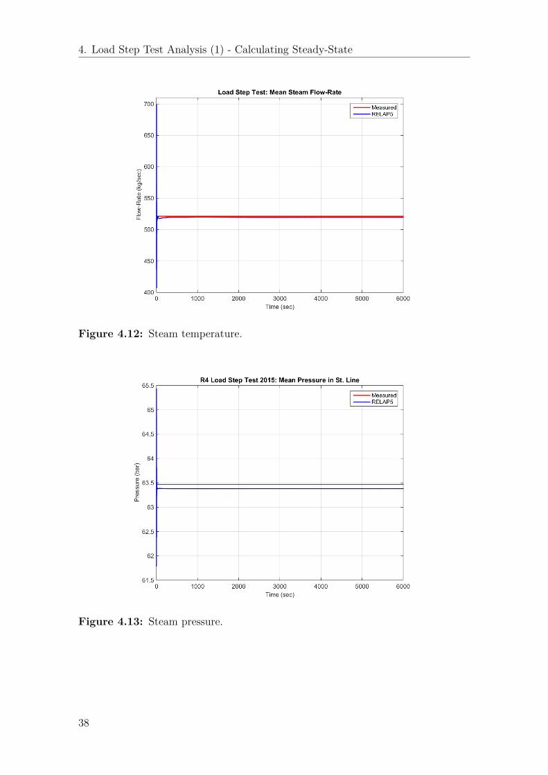
Figure 4.12: Steam temperature.

Figure 4.13: Steam pressure.

38


It can be concluded from table 4.1 and from the figures above that all the variablesconverge during the 6000 s duration of the steady-state runs. Some of them, likethe pressure in the steam lines (figure 4.13) and the pressure in the SGs (figure4.3), converge fast, whereas others, like the hot leg temperature (figure 4.9) andthe pressure in the PRZ (figure 4.5) need thousands of seconds to converge. Thegoal of reaching a realistic steady-state by the code is fulfilled. The next step is theinitiation of the transient runs, each of 4500 sec duration, starting from the end ofthe most successful steady-state run presented above.

39


40

5Load Step Test Analysis (2) -

Transient Analysis

Analysis of the whole transient takes place in this chapter. Transient runs begin atthe end of the steady-state runs. After each run the calculated results are comparedagainst the test data. Experience has shown that when the calculated secondarypressure matches with the corresponding measured values, the other variables tendto converge to their measured values as well. Hence, the first thing to check aftereach run is the pressure in the SGs. The turbine control valve opening is adjustedmanually due to the lack of turbine valve characteristic curve, so that the calculatedsecondary pressure matches with the corresponding one from the test data.

The first issue to be discussed in the following sections of this chapter is thethermal power ratio. Defining a realistic power ratio during the transient is one ofthe most challenging issues when performing transient runs. Then, some issues withthe PRZ control systems found during the transient runs are discussed as well asthe way they were tackled. Finally, the results of the best transient run, with thecorresponding corrections of the model are presented.

5.1 Thermal Power RatioThe current model is a "stand alone" thermohydraulic model and the time evolutionof the thermal power level is not determined in a coupled neutron kinetic code.Consequently, the thermal power is user given input in a general table in the model.It is very important to give a table with realistic thermal power values as functionof time in order to produce better results as possible. However, as it was underlinedin the previous paragraphs, the thermal power is the most determining parameter,which has the strongest influence on the calculated results.

41

5. Load Step Test Analysis (2) - Transient Analysis

Three approaches were tested to derive the thermal power:1. Set the thermal power ratio equal to the neutron flux/neutronic power (%)

plant data. This is equivalent to assume linear interdependence between neu-tron flux and thermal power. The results are presented in figure 5.1.

2. Calculate the thermal power ratio by calculating the enthalpies of the feedwa-ter and of the steam produced. Using the test data for pressure and feedwater,its enthalpy is calculated using water property tables. The enthalpy of the pro-duced steam is calculated using steam properties table for quality x = 1 andthe measured steam pressure values during the whole transient. Hence, thethermal power is calculated as:

Qtot =3∑

i=1QSG,i = 3 × mfw(hsteam − hfw)

where the quantity mfw(hsteam − hfw) is the thermal power produced by oneSG. The thermal power along the transient is normalized with the time av-erage of the calculated power using the above equation, from 0 to 338s. Thecalculated thermal power ratio is presented in figure 5.2.

3. Using the fact that Q = mcp∆T it means that the thermal power ratio will bevarying proportional to the temperature difference ∆T = THL − TCL betweenthe hot and cold leg. The temperature difference between the hot and coldleg is calculated using the corresponding test data for the whole transient, andis normalized with the average of the temperature differences from 0 to 338s.The results are presented in figure 5.3.

Among the three fore-mentioned approaches the third one leads to better results.A quick look in figure 5.3 shows that the steam production/steam flow-rate behavein the same manner as the thermal power ratio. More thermal power translates intomore steam and the opposite, as ones physical intuition dictates, which does nothappen in the two previous approaches. In the first one, the thermal power ratio istilted compared to the steam production during the intermediate steady-state. Inthe second half of the intermediate steady-state less thermal power produces thesame amount of steam as in the first half with more thermal power. This is quiteunphysical. In last part of the transient, after the power uprate the thermal powerdoes not follow the steam production trend either. The second approach is incapableof reflecting the first seconds of the intermediate steady-state as well as the last partof the transient after the power increase.

As long as the thermal power ratio during the transient is set, then a power ratiotable for 99 time entries (RELAP5 confinement) is built using the thermal powerratio from ∆T .

42


Figure 5.1: Steam flow-rate and thermal power ratio used in the calculation. Thethermal power ratio is deduced from the neutron flux test data.

Figure 5.2: Steam flow-rate (left axis) and thermal power ratio used in the calcu-lation. The thermal power ratio is calculated using the feedwater flow-rate and theenthalpies of the feedwater and of the steam.

43


Figure 5.3: Steam flow-rate (left axis) and thermal power ratio used in the calcu-lation. The thermal power ratio is calculated based on the temperature differencebetween the hot and the cold leg.

5.2 Discrepancies in the PRZDuring the transient runs discrepancies in the calculated pressure and level in thePRZ have occurred (figures 5.5 and 5.6). In figure 5.5 it is observed that there arerelatively high discrepancies during the power increase phase, roughly between 500and 1500 s. During this time interval a high pressure overshoot takes place comparedwith the test data. Relatively high overshoots are observed in figure 5.6 between500 and 1500 s as well. Likewise, in the second half of the intermediate steady-stateand after that, the code cannot predict the measured level values as accurate as inthe first phase of the transient. Not to mention that the calculated spraying controlsignal is half of the corresponding measured values during the power increase (figure5.7).

Given that the PRZ pressure controllers have been checked and refined duringthe steady-state runs, the discrepancies in the spraying control signal indicate thatthe PRZ level controller may be a source of these discrepancies. The discrepancies inthe calculated water level in the PRZ could originate due to overfeeding or improperfeeding by the chemical and volume control system (CVCS), and thus, of the feedingflow (figure 5.4). A question may arise that what if the charging flow-rate or thespraying control signal would be equal to the corresponding test values? Would iteliminate the discrepancies in the calculated PRZ pressure and level?

44


In order to answer these questions, the code has been run for two different cases:1. Manual spraying flow-rate and automatic charging flow-rate.2. Manual charging flow-rate and automatic spraying flow-rate.The second approach, the manual water charging of the primary side drastically

improves all the results and consolidated the initial suspicion of poor documentationof the PRZ controllers, especially the of the PRZ level controller. Thus, it is decidedto go along with manual charging water injection in the primary side for the rest ofthe transient calculations.

Figure 5.4: Charging flow-rate in the primary side. Discrepancies occur duringthe whole transient, however they intensify during the sharp thermal power decreaseand increase.

45


Figure 5.5: Pressure in the PRZ. Noticeable discrepancies occur between 500 and1500 s as well as after 4000 s.

Figure 5.6: Water level in the PRZ. Noticeable discrepancies after 500 s.

46


Figure 5.7: Output of spraying flow-rate controller. This control signal is trans-lated into spraying flow-rate through the valve characteristic curve.

5.3 Transient Analysis ResultsIn the last series of transients runs the RELAP5 table of feedwater temperatureis readjusted so as to capture the decrease of feedwater temperature during theintermediate steady-state.

Despite the fact that feedwater temperature changes roughly 4 K it seems thatit affects the heat balance of the system and improves the calculated results whensimulated.

It should also be noted that the length of the charging line is set equal with 10m. Its previous value was 100 m an old estimate by the original developer of thecode. The 100 m value for the length of the charging line seem to be exaggeratedand that is the reason of its replacement with the most realistic 10 m value.

The results of the most successful transient run are presented in the followingpages.

47


Figure 5.8: Thermal Power input for the transient runs.

Figure 5.9: Pressure in the pressurizer.

48


Figure 5.10: Level in the PRZ.

Figure 5.11: Pressure in the SG.

49


Figure 5.12: Level in the SG.

Figure 5.13: Temperature in hot leg.

50


Figure 5.14: Temperature in cold leg.

Figure 5.15: Loop average temperature.

51


Figure 5.16: Feedwater flow-rate in the secondary side.

Figure 5.17: Steam flow-rate.

52


Figure 5.18: Charging flow-rate (given as boundary condition).

Figure 5.19: Proportional heaters capacity.

53


Figure 5.20: Spraying flow-rate signal.

The calculated values follow the trend of the test values and that almost allvariables are predicted with very good precision. However, in some cases, like thefeedwater flow (figure 5.16) overshooting is observed, not significant though, duringthe sharp power decrease and increase phases of the transient. However, a morethorough assessment of the accuracy of the code predictions is given by the FFTBMwith signal mirroring in the following chapter.

5.4 Transient Analysis Concluding RemarksThe charging flow-rate is set as a boundary condition. This approach is followedin order to show that the results produced with charging flow set as boundaryconditions are better than those when the charging flow is regulated automaticallyby the PRZ control systems. It is believed that improper modelling of the PRZ levelcontroller mostly affects negatively the accuracy of the calculated results.

For manual charging flow-rate the calculated results seem to follow the trendof the corresponding test data and the vast majority of the variables are predictedwith very small error, like the primary pressure (figure 5.9) and the loop averagetemperature (figure 5.15). Some others are predicted with a relatively higher errorwhich are still between the acceptability limits. For instance, the steam flow- ratesduring the intermediate steady-state are predicted with relative error less than 5 %.

As for the spraying flow-rate signal concerned, it seems that despite the fact thatthe calculated results follow the trend of the test values, the peak of the sprayingduring the power decrease is not predicted as accurately as other variables, like theprimary pressure. This happens because the calculated control signal decays slowerthan the actual one (not visible in figure 5.20). Again, this has to do with the PRZ

54


controllers inadequate modelling.However it should be noted that mass flow-rates in general are one of the most

difficult values to be predicted by BE-codes.

55


56

6Accuracy Quantification usingFast Fourier Transform Based

Method (FFTBM)

Quite often BE-code users have to deal with the following questions [22]:• How many simplifications can the model afford without deteriorating the pre-

diction accuracy?• What is the margin for necessary improvements in the model?• How to perform an objective assessment of the model?FFTBM is a method that deals with the above questions by depicting the discrep-

ancies between the calculated and the experimental data in the frequency domain.It provides the means to assess the "goodness" of the method.

So far, FFTBM has been applied to primary side transients, especially for SB-LOCAs simulations in small-scaled facilities, secondary side transients as well as inburn-up calculations assessment.

6.1 FFTBM Outline

FFTBM is using Fast Fourier Transformation algorithm (FFT) in order to calculatethe Discrete Fourier Transformation (DFT) of the experimental calculated signals.Thus, N samples from the experimental/calculated signals are needed. When FFTis used, in order for the sampling theorem to be fulfilled (the number of samplesneeded in order the experimental/calculated signal to be reliably represented by thesampled values) N = 2m+1,m = 8, 9, 10, 11. Hence, the sampling frequency readsas:

1τ

= fs = 2fmax = N

Td

= 2m+1

Td

,

where Td is the duration of the sampled signal, τ the time interval between twosuccessive samples and fmax the highest frequency component of the signal. Thesampling theorem does not hold beyond fmax.

6.1.1 Average AmplitudeAverage Amplitude AA is the basic measure used for FFTBM analysis. Supposingthat the difference between the calculated Fcal(t) signal and the experimental one

57

6. Accuracy Quantification using Fast Fourier Transform Based Method (FFTBM)

Fexp(t) reads in the time domain as: ∆F = Fcal(t) − Fexp(t) then, the averageamplitude AA is calculated as:

AA =∑2m

n=0 ∆F (fn)∑2m

n=0 Fexp(fn),

where ∆F (fn) and Fexp(fn) the DFT of ∆F and Fexp as calculated by FFT algorithmrespectively. AA can be interpreted as an integral measure that keeps track ofthe relative magnitude of the discrepancy between the experimental and calculatedvariable over the time history. Calculating the AA value of a variable of interest thefollowing conclusions can be made for its prediction by the code:

• AA ≤ 0.3 corresponds to very good variable prediction.• 0.3 < AA ≤ 0.5 corresponds to good variable prediction.• 0.5 < AA ≤ 0.7 corresponds to poor variable prediction.• AA > 0.7 corresponds to very poor variable prediction.This criterion refers to one variable. Usually, it is favorable to quantify the

overall model accuracy based on a number of different variables Nvar. Thus, thetotal average amplitude AAtot for all of the variables of interest can be computedas:

AAtot =Nvar∑i=1

(wf )i(AA)i

where (wf )i the weighting factor of the i−th variable of interest. The above criterionin this case is modified as:

• AAtot ≤ 0.34 corresponds to very good code prediction.• 0.3 < AAtot ≤ 0.5 corresponds to good code prediction.• 0.5 < AAtot ≤ 0.7 corresponds to poor code prediction.• AAtot > 0.7 corresponds to very poor code prediction.There is a certain limit for the AA or AAtot that should not be overwhelmed for

experienced users, the so called "acceptability limit" AA < 0.4.Those weighting factors are normalized, thus:

Nvar∑i=1

(wf )i = 1

The weighting factor (wf )i of the i− th variable of interest is subsequently definedas:

(wf )i = (wexp)i(wsaf )i(wnorm)i∑Nvari=1 (wexp)i(wsaf )i(wnorm)i

where (wexp)i accounts for the uncertainty due to the instrumentation or of themeasurement method, (wsaf )i the safety relevance of the variable, and (wnorm)i theinterrelation with the primary pressure since in a complex system like a nuclearreactor variables are not completely independent with each other. Primary pressureis a variable of significant importance therefore it is used as a benchmark for fixing(wnorm)i values for different variables. Weighting factors (wexp)i, (wsaf )i and (wnorm)i

are usually referred to as experimental accuracy, safety relevance and primary pres-sure normalization respectively. These three weighting factors are not normalized

58


usually. Their values are a subject of engineering judgment, which introduces adegree of arbitrariness, and as long as their values have been decided for a partic-ular transient they should not be changed when comparing different codes/modelsresults. FFTBM was first introduced for SB-LOCAs and the weighting factors werefirst estimated for this kind of transient, as shown in table 6.1.

Quantity wexp wsaf wnorm

Pressure Drops 0.7 0.7 0.5Mass Inventories 0.8 0.9 0.9Flow-Rates 0.5 0.8 0.5Primary Pressure 1.0 1.0 1.0Secondary Pressure 1.0 0.6 1.1Fluid Temperatures 0.8 0.8 2.4Clad Temperatures 0.9 1.0 1.2Collapsed Levels 0.8 0.9 0.6Core Power 0.8 0.8 0.5

Table 6.1: Weighting factors for different measured quantities (SB-LOCA) [8, 12,22].

6.1.2 Additional Measures for Accuracy QuantificationAdditional measures used in FFTBM analysis are the variable accuracy V Ai of thei − th variable of interest, the minimal and maximal variable accuracy V Amin andV Amax respectively, as well as the number of discrepancies ND [8, 18].

Variable accuracy V Ai of the i − th variable of interest shows what the totalaverage amplitude AAtot would be if the rest of the chosen variables all have thesame weighting factor (wf )i and average amplitude AAi. Therefore it is designatedas:

V Ai = (wf )i · AAi ·Nvar

It should be mentioned that the criterion for AA is applicable for V Ai too.Minimal variable accuracy V Amin and maximal variable accuracy V Amax indicatethe minimum and the maximum variable accuracy among the accuracy amplitudesAAi, i = 1, . . . , Nvar of the Nvar chosen variables.

Consequently, they are defined as:

V Amin = max(V Ai), i = 1, . . . , Nvar

andV Amax = min(V Ai), i = 1, . . . , Nvar

As it is mentioned before the acceptability limit is 0.4 and consequently AAtot < 0.4.Hence, the number of discrepancies ND is equal with the number of variables forwhich V Ai > 0.4. It is obvious that ND = 0 when V Amin < 0.4. It should bementioned that a prerequisite for the application of FFTBM is that the averageamplitude of the primary pressure is AA < 0.1 due to the significant influence ofthis variable in the system.

59


6.2 Methodology for Code Accuracy Quantifica-tion

Initially, a qualitative assessment of the code results should take place to see whetherthe code predicts accurately the measured data and whether the calculated resultsfollow the trend of the measured ones.

Then, the transient is divided in phenomenological windows for which the relevantthermal-hydraulic aspects (RTA) are identified (most important events/phenomenaoccurring). Variables that best describe the RTA are chosen. Then the weightingfactors of the variables are set. The average amplitude AA of each chosen variableas well as the AAtot can be calculated using the increasing time window approach.

In increasing time window approach the transient is divided in equal and succes-sive time slots. Increasing time windows are then made by adding successive timeslots so that the first time window corresponds to the first time slot, the secondtime window to the addition of the two first time slots etc. Hence, the last timewindow corresponds to the whole duration of the transient. AAi for i = 1, . . . , Nvar

and AAtot are calculated for each time window and plotted with time. This is thenew increasing time window approach proposed in [8].

In the old increasing time window approach [22] the transient used to be par-titioned in time slots equal with the duration of each phenomenological window.The time windows were constructed in the same manner as mentioned above, byadding successive time slots. Nonetheless, the new increasing time window approachallows to better track the evolution of AAi or AAtot with time, especially for tran-sients with few phenomenological windows. In addition it reveals when the biggestdiscrepancies occur and their contribution both to variable and total accuracy.

In addition, the discrete calculated and discrete experimental signal are mirroredin the time domain in order to avoid an inherent weakness of the original FFTBMmethod that produced unphysical AA results [10]. AA (AAi or AAtot) should in-crease with increasing time window, since it is an integral discrepancy measurethroughout the increasing time window interval. Consequently as time window in-creases, addition of discrepancies of the newly added time slots occur, which is whyAA should monotonically increase. However this does not happen when the last andthe first point of the discrete signal differ significantly. FFT multiplies the discretesignal so as to create a periodic infinite signal. As a result, any difference betweenthe first sample of each period with the last sample of the previous period increasesthe frequency content of AA, distorting it significantly.

6.3 FFTBM AnalysisThe quantitative analysis is described in the Transient Analysis (2) - TransientResults chapter. The main conclusion of the qualitative analysis is that overall thecalculated results are in very good agreement with the corresponding experimentalvalues.

60


Then, FFTBM with signal mirroring is applied for the quantification of the good-ness of the model used mainly through average amplitude AA.

The transient is partitioned in five phenomenological windows:1. Initial Steady-State, 0 − 338 s2. Power Decrease, 338 − 500 s3. Intermediate Steady-State, 500 − 3914 s4. Power Increase, 3914 − 4300 s5. Stabilizing in the Initial Steady-State, 4300 − 4500 sA number of 25 variables descriptive of the most important RTA were chosen

for the assessment, those that appear as inputs or outputs in the PRZ level andpressure controllers as well as in SG level controller (table 6.2).

The safety and experimental weighting factors used are the same as the onesused for the SB-LOCA transient. The normalised factors are chosen as the aver-age amplitude for each variable divided by the average amplitude of the primarypressure.

For the FFTBM analysis JSI FFTBM Add-in 2007 is used. It is an Excel-2007add-in developed by Jožef Stefan Institute in Ljubljana by Dr. Andrej Prošek. Theuser should tabulate the experimental as long as the calculated data. The optionsprovided by the add-in is FFTBM with or without signal mirroring, Safety AnalysisReport (SAR) analysis and plotting of the experimental versus the calculated data.

6.4 FFTBM ResultsThe results for the biggest time window 0−4500 s are representative of the variablestrends during the whole transient and they are presented in table 6.2. From figure6.1 it can be seen that the primary pressure criterion AA < 0.1.

The evolution of total average accuracy AAtot is depicted in figure 6.12. It canbe seen that the total average accuracy is below the acceptability limit and that theoverall predictions of the code are good.

The number of discrepancies (variables with V A > 0.4) in the 0 − 4500 s timewindow is equal to 5, which is due to the steam flow-rates, the spraying flow-ratesignal and the proportional heaters capacity.

However, from the figures and from the AA - V A data in table 6.2 it can beseen that the spraying flow-rate signal (figure 6.11) is the variable with the mostdeleterious influence in total average accuracy. Its AA and V A are well above theacceptability limit.

The second variable that negatively influences the code accuracy is the propor-tional heaters capacity (figure 6.10) and last, the steam flow-rates figure(6.9). Thebehaviour of spraying and of the proportional heaters substantiates the suspicionsfor the controllers modelling.

Seventeen variables have AA ≤ 0.1. Hence their prediction is excellent and it isvery noticeable that among those variables the most important system variables areincluded. Namely, the primary pressure, the secondary pressure, the levels of theSGs and of the PRZ, and all temperatures.

61


V ariable Weightingfactors 0 − 4500swexp wsaf wnorm AA V A

Primary Pressure 1.0 1.0 1.0 0.02 0.006Level in PRZ 0.8 0.9 4.1 0.09 0.1Pressure in SG-1 1.0 0.6 1.1 0.02 0.004Pressure in SG-2 1.0 0.6 1.3 0.03 0.005Pressure in SG-3 1.0 0.6 1.2 0.03 0.004Level in SG-1 0.8 0.9 4.2 0.09 0.07Level in SG-2 0.8 0.9 4.5 0.10 0.08Level in SG-3 0.8 0.9 4.3 0.10 0.08Hot Leg Temp. in Loop 1 0.8 0.8 0.3 0.02 0.001Hot Leg Temp. in Loop 2 0.8 0.8 0.4 0.02 0.001Hot Leg Temp. in Loop 3 0.8 0.8 0.4 0.02 0.001Cold Leg Temp. in Loop 1 0.8 0.8 11.7 0.01 0.02Cold Leg Temp. in Loop 2 0.8 0.8 11.1 0.01 0.02Cold Leg Temp. in Loop 3 0.8 0.8 11.8 0.01 0.02Average Temp. in Loop 1 0.8 0.8 0.3 0.008 0.0004Average Temp. in Loop 2 0.8 0.8 0.4 0.008 0.0004Average Temp. in Loop 3 0.8 0.8 0.4 0.008 0.0004Feedwater Flow in SG-1 0.5 0.8 11.7 0.26 0.30Feedwater Flow in SG-2 0.5 0.8 11.1 0.25 0.27Feedwater Flow in SG-3 0.5 0.8 11.8 0.27 0.31Spraying Control Signal 0.5 0.8 43.1 0.97 4.15Prop. Heaters Capacity 0.8 0.8 19.7 0.44 1.39Steam Line - 1 Flow 0.5 0.8 14.1 0.32 0.44Steam Line - 2 Flow 0.5 0.8 16.1 0.36 0.58Steam Line - 3 Flow 0.5 0.8 14.9 0.33 0.50Total 0.33

Table 6.2: FFTBM analysis variables, weighting factors and results for the 0−4500s interval

From the total accuracy figure (figure 6.12) and from the spraying flow-rate signalfigure (figure6.11) it can be deduced that it is mostly the discrepancies during thefirst spraying period that contributes negatively to the accuracy of this variable andto the total accuracy. In other words the big jump in AAtot diagram is caused bythe jump occurring in the AA of the spraying flow-rate signal. In the same trendthe discrepancies of every variable during the power decrease phase are greaterthan in the rest of the transient, especially compared to the discrepancies occurringduring the power increase phase. It seems that the modeled control systems areinitially "shocked" due to the power decrease but then they manage to compensatethe transient.

62


Figure 6.1: Average amplitude of the primary pressure.

Figure 6.2: Average amplitude of level in the PRZ.

63


Figure 6.3: Average amplitudes of the pressure in the SGs.

Figure 6.4: Average amplitudes of the levels in the SGs.

64


Figure 6.5: Average amplitudes of the hot leg temperatures in the SGs.

Figure 6.6: Average amplitudes of the cold leg temperatures in the SGs.

65


Figure 6.7: Average amplitudes of the average loop temperatures.

Figure 6.8: Average amplitudes of the feedwater flow-rates in the SGs.

66


Figure 6.9: Average amplitudes of the steam flow-rates in the SGs.

Figure 6.10: Average amplitude of the proportional heaters capacity.

67


Figure 6.11: Average amplitude of the spraying flow-rate signal.

Figure 6.12: Total average amplitude.

68


6.5 FFTBM Analysis Concluding RemarksIn general, on the basis of the FFTBM analysis it can be concluded that the codepredictions of the most important parameters, like the primary and secondary pres-sure are excellent.

Figure 6.12 indicates that the quality of overall code predictions are in the rangeof good agreement. Yet, there is a margin for further improvement by re-examinationand possible re-adjustment of the modeled PRZ controllers, especially the PRZ levelcontroller.

69


70

7Conclusion

This chapter presents the most important results of the previous analysis and arecommendation for future work is given.

7.1 Summary - Main ConclusionsThe main purpose of the Load Step Test is to check the ability of the control systemsto handle the perturbations without triggering any safety or protection systems.This should also be reflected in the simulation of the Load Step Test by the RELAP5model of Ringhals 4, which is successful.

The first step for the simulation of the transient is that the code is able to achievea steady-state close to one of the real reactor. The code reaches a steady-state after6000 s and the steady-state values of the most important variables predict thecorresponding test data values.

Thermal power level throughout the transient is the most important parameteraffecting the calculated results. Deriving it from the temperature difference betweenthe hot and the cold legs is the most reliable way.

Investigation of the calculated PRZ level discrepancies revealed that the causelied in the inappropriate modeling of the CVCS system which affected the feedingflow of the PRZ from the surge line as well as the spraying flow. Hence, the remainingtransient calculations were run with the primary side charging flowrate given as aboundary condition.

The FFTBM analysis shows the overall reliability of the code predictions. Thepredictions of the most important variables, 20 out of the 25 chosen variables, canbe labeled as very good. The predictions for the spraying control signal and theproportional heaters are not satisfactory. The last two indicate that the modellingof the PRZ controllers has to be improved. Thus, additional data like spraying valvecharacteristics will be needed.

7.2 Proposals for Future WorkThe work presented above revealed the inappropriate modelling of the PRZ level con-trol system (CVCS). Consequently, the most important recommendation for futurework is the re-examination of the PRZ control system because this will contributeto the improvement of the results.

71

7. Conclusion

The weighting factors that were set for the FFTBM analysis of the Load StepTest are presented in table 6.2. As it is mentioned in a previous chapter, the weight-ing factors are set for different transient types and their values are a subject ofengineering judgement. It would be useful to further if more appropriate weightingfactors could be set.

Furthermore, development of a PARCS neutron kinetic model for Ringhals 4which will be coupled with the existing RELAP5 model will pave the way for a morecomplete and integrated neutronic-thermalhydraulic model of Ringhals 4, increasingthe model fidelity and ultimating the ability of transient predictions.

Another option for future work is the conversion of RELAP5/MOD3.3 model ofRinghals 4 to TRACE, which is a new and more user-friendly code compared toRELAP5.

72

Bibliography

[1] Information Systems Laboratory Inc., RELAP5/MOD3.3 Code Manual, Vol-ume II: User’s Guide and Input Requirements, 2010, US Nuclear RegulatoryCommission.

[2] Information Systems Laboratory Inc., RELAP5/MOD3.3 Code Manual VolumeV: User’s Guidelines, 2010, US Nuclear Regulatory Commission.

[3] Ringhals 4-Frej Project-Software Settings.[4] J. Bánáti, A. Stathis Validation of the RELAP5 Model of RINGHALS 4 against

a Load Step Test at Uprated Power", Chalmers University of Technology, De-partment of Applied Physics, Division of Nuclear Engineering, 2015.

[5] J. Bánáti, Technical Description of the RELAP5 Model forRINGHALS 4 NPP,Chalmers University of Technology, Department of Applied Physics, Divisionof Nuclear Engineering, 2013.

[6] A. Agung, J. Bánáti, M. Stålek, C. Demaziere, Validation of PARCS/RELAP5coupled codes against a load rejection transient at the Ringhals-3 NPP, NuclearEngineering and Design, 2013, vol.257, p.31-44.

[7] J. Bánáti, Validation of the RELAP5 Model of RINGHALS 4 against the 2011-12-14 ± 10 % Load Step Test", Chalmers University of Technology, Departmentof Applied Physics, Division of Nuclear Engineering, 2013.

[8] A. Prošek, B. Mavko", Quantitative Code Assessment with Fast Fourier Trans-form Based Method improved by Signal Mirroring, Nuclear Regulatory Com-mission, NUREG/IA-0220, December 2009.

[9] H. Glaeser CSNI Integral Test Facility Matrices for validation of Best EstimateThermal-Hydraulic Computer Codes, THICKET 2008-Session III-Paper 04.

[10] A. Prošek, M. Leskovar, B. Mavko, Quantitative Assessment with improved fastFourier transformed based method by signal mirroring, Nuclear Engineering andDesign, 2008, vol.238, p.2668-2677.

[11] A. Petruzzi, F. D’Auria, Thermal Hydraulic System codes in Nuclear ReactorSafety and Qualification Procedures, Science and Technology of Nuclear Instal-lations, 2008.

[12] A. Prošek, JFI FFTBM Add-in 2007 Users Manual, Jožef Stefan Institute,Ljubljana, December 2007.

[13] M. J. Moran, H. N. Shapiro, Fundamentals of Engineering Thermodynamics,5th Edition, SI Units, John Wiley Sons, 2006.

[14] A.Prošek, F. D’Auria, D. J. Richards, B. Mavko, Quantitative assessment ofthermal-hydraulic codes used for heavy water reactor calculations, Nuclear En-gineering and Design, 2006, vol.236, p.295-308.

73

Bibliography

[15] A.Prošek, FFTBM and Primary Pressure Acceptance Criterion, Nuclear En-ergy for New Europe International Conference-2004, 2004, Portoro, Slovenija.

[16] J. Lillington, The future of Nuclear Power, Elsevier, 2004.[17] M. Schleicher, F. Blasinger, Control Engineering, a Guide for Beginners, 3rd

Edition, JUMO GmbH Co. KG, 2003.[18] A. Prošek, B. Mavko, A tool for Quantitative assessment of code calculations

with an improved fast Fourier transform based method, Elektrotehniški vestnik,2003.

[19] J. Wilkie, M. Johnson, R. Katebi, Control Engineering, an Introductory Course,Palgrave Macmillan, 2002.

[20] A.Papaioannou, Fluid Mechanics, Vol. 2, (in Greek), Korali, 2002.[21] A.Prošek, Lessons Learned from Accuracy Assessment of IAEA-SPE-4 Exper-

iment Predictions, Nuclear Energy for New Europe International Conference-2002, 2002, Kranjska Gora, Slovenija.

[22] A. Prošek, F. D’Auria, B. Mavko, Review of Quantitative Accuracy Assessmentwith Fast Fourier Transform Based Method (FFTBM), Nuclear Engineeringand Design, 2002, vol.217, p.179-206.

[23] N. E. Todreas, M. S. Kazimi, Nuclear Systems II, Elements of Thermal Hy-draulic Design, Taylor Francis, 2001.

[24] B. Preshagen, Light Water Reactor Safety, Pergamon Press, 1998.[25] B. Mavko, A. Prošek, F. D’Auria, Determination of code accuracy in predicting

small break LOCA experiment, Nuclear Engineering and Design, 1997, vol.120.[26] N. E. Todreas, M. S. Kazimi, Nuclear Systems I, Thermal Hydraulic Funda-

mentals, Taylor Francis, 1993.[27] S. N. Aksan, F. D’Auria, H. Städke, User Effects on the thermal-hydraulic tran-

sient system code calculations, Nuclear Engineering and Design, 1993, vol.245,p.159-174.

[28] S. N. Aksan, F. D’Auria, H. Städke, CSNI code validation matrix of thermo-hydraulic codes for LWR LOCA and transients, Committee on the safety ofnuclear installations, OECD Nuclear Energy Agency, 1987.

[29] Westinghouse Electric Corporation, Water Reactor Divisions, The Westing-house Pressurized Water Reactor Nuclear Power Plant, 1984.

[30] IAEA country nuclear profiles: Sweden, 2015 edition,http://www-pub.iaea.org/MTCD/Publications/PDF/CNPP2015_CD/countryprofiles/Sweden/Sweden.htm

[31] PWR diagram,http://www.edusolution.com/current_issues/nuclear/nuclear3

[32] IAEA country nuclear profiles: Sweden, 2015 edition,http://www-pub.iaea.org/MTCD/Publications/PDF/CNPP2015_CD/countryprofiles/Sweden/Sweden.htm

74

http://www-pub.iaea.org/MTCD/Publications/PDF/CNPP2015_CD/countryprofiles/Sweden/Sweden.htm


http://www.edusolution.com/current_issues/nuclear/nuclear3



Date post:	23-May-2018
Category:	Documents
Upload:	vokhue
View:	215 times
Download:	2 times

Analysis of a Load Step Test at Ringhals 4 NPP using...

Documents