ANALYSIS OF PANEL PATENT DATA USING POISSON, NEGATIVE BINOMIAL AND GMM ESTIMATION BY Qi Hu B.E. Dalian University of Technology, 1996 M.Mgmt. Dalian University of Technology, 2000 A PROJECT SUBMITTED IN PARTIAL FULFILLMENT OF THE REQUIREMENTS FOR THE DEGREE IN MASTERS OF ARTS In The Department Of Economics O Qi Hu 2002 SIMON FRASER UNIVERSITY July 2002 All rights reserved. This work may not be reproduced in whole or in part, by photocopy or other means, without permission of the author.
Transcript
ANALYSIS OF PANEL PATENT DATA USING POISSON,
NEGATIVE BINOMIAL AND GMM ESTIMATION
BY
Qi Hu
B.E. Dalian University of Technology, 1996
M.Mgmt. Dalian University of Technology, 2000
A PROJECT SUBMITTED IN PARTIAL FULFILLMENT OF THE
REQUIREMENTS FOR THE DEGREE IN MASTERS OF ARTS
In The Department Of Economics
O Qi Hu 2002 SIMON FRASER UNIVERSITY
July 2002
All rights reserved. This work may not be reproduced in whole or in part, by photocopy or other means, without
permission of the author.
APPROVAL
Name: Qi Hu
Degree: M. A. (Economics)
Title of Project: Analysis Of Panel Patent Data Using Poisson, Negative Binomial And GMM Estimation
Examining Committee:
Chair: Brian Krauth
\ 1 T
Peter Kennedy Senior Supervisor
Terry Heaps Supervisor
r Ken Kasa Internal Examiner
Date Approved: Friday July 26,2002
. . 11
PARTIAL COPYRIGHT LICENSE
I hereby grant to Simon Fraser University the right to lend my thesis, project or extended
essay (the title of which is shown below) to users of the Simon Fraser University Library,
and to make partial or single copies only for such users or in response to a request from
the library of any other university, or other educational institution, on its own behalf or
for one of its users. I further agree that permission for multiple copying of this work for
scholarly purposes may be granted by me or the Dean of Graduate Studies. It is
understood that copying or publication of this work for financial gain shall not be
allowed without my written permission.
Title of Project Analysis Of Panel Patent Data Using Poisson, Negative Binomial And GMM Estimation
Author:
Qi
ABSTRACT
The relationship between patent applications and R&D expenditure is a prominent
example of a count data model with panel data. This paper examines the patents-R&D
relationship by estimating three different panel count data models. The data includes 346
firms from 1970 to 1979. First is the Poisson model. Since we have panel data, fixed
effects and random effects models are developed to allow individual firms to have their
own average propensity to patent. Then a more commonly used model, the negative
binomial model, is estimated to allow for overdispersion which typically characterizes
data of this form. The results from these two models are compared using an
overdispersion test and a Hausman test. The fixed effect negative binomial model is
found to be the superior model. These two models assume strict exogeneity of the
explanatory variables. Estimation via GMM is undertaken to address this problem.
DEDICATION
DEDICATED TO MY FAMILY
ACKNOWLEDGEMENTS
I would like to take this opportunity to express my gratitude to my senior supervisor,
professor Peter Kennedy for his invaluable guidance and encouragement throughout the
process of my graduate work. I also thank Professor Terry Heaps, from whom I learned
much about how to write this project in a professional manner. Many thanks to Dr.
Xiannian Sun for his many suggestions on the project. I am also grateful to the faculty
and staff at the SFU Economics Department, for their assistance during my graduate
DEDICATION .............................................................................................................. iv
................................................................................................. ACKNOWLEDGEMENTS v
TABLE OF CONTENTS ............................................................................................ vi
LIST OF TABLES AND FIGURES .............................................................................. vii
I INTRODUCTION .......................................................................................................... 1
I1 LITERATURE REVIEW ............................................................................................ 2
I11 BASIC POISSON REGRESSION MODEL ............................................................. 4
................................................................... 3.1 THE BASIC POISSON REGRESSION MODEL 4 ................................................................................................... 3.2 DATA DESCRIPTION 5
3.3 EMPIRICAL RESULTS OF BASIC POISSON MODEL ...................................................... 6
IV PANEL POISSON REGRESSION MODEL ............................................................ 7
.......................................................................... 4.1 RANDOM EFFECTS POISSON MODEL 8 4.2 FIXED EFFECTS POISSON MODEL .............................................................................. 9
........................................... 4.3 EMPIRICAL RESULTS FOR THE PANEL POISSON MODEL 10
V NEGATIVE BINOMIAL MODEL Ah?) OVERDISPERSION TEST ................. 11
5.1 PANEL NEGATIVE BINOMIAL MODEL .......................................................... 12 ..................................................................................... 5.2 -ST FOR OVERDISPERSIO~' 13
TABLE 6 ESTIMATES OF NEGATIVE BINOM~AL MODEL .................................................. 14
VI HAUSMAN TEST ..................................................................................................... 15
VII GMM ESTIMATION .............................................................................................. 16
....................................................... 7.2 EMPIRICAL RESULT USING GMM ESTIMATION 19 ..................................................................................... 7.3 OVERIDENTIFICATION TEST 20
VIII CONCLUSION ....................................................................................................... 21
APPENDIX I ................................................................................................................... 23
......................................................... Definition of Variables
Descriptive Statistics of Variables .......................................... ....................................... Estimates of the Basic Poisson Mode 1
........................ Estimates of Panel Poisson Model with Random Effects
Estimates of Panel Poisson Model with Fixed Effects ........................... .................................... Estimates of Negative Binomial Model
The Result of The GMM Estimation ................................................ Comparison of Alternative Estimatiors ....................................
vii
I INTRODUCTION
The main focus of this paper is to apply different panel count data models to conduct an
empirical study on the relationship between Patent applications and R&D expenditures,
and to find a better model. For the period of 1970 to 1979 there are 346 firms whose
annual data are used for this study. A simple "Poisson model" is employed first given the
non-negative and discrete nature of the number of patent applications. Since we have
panel data, fixed and random effect Poisson models are applied as well. In addition, we
applied the negative binomial model in order to offset the strong assumptions of the
Poisson models. Our finding was that the negative binomial model with fixed effects
outperforms the other models. To avoid some assumptions that may fail in the context, an
empirical analysis by the generalized method of moments (GMM) is also carried out in
the last part.
The rest of the paper is organized as follows: Section I1 reviews the study of patent-R&D
expenditure relationship in the open literature. Section I11 provides a brief review of the
assumptions of the basic Poisson model and applies this model to the data in order to
obtain a benchmark result. Data description is also included in this part. Section IV takes
into consideration the nature of the panel data. Fixed and random effect models are
applied to allow each individual firm to have its own average propensity to patent.
Section V tests for 'overdispersion' in the data as usually the assumption of equal mean
and variance may be unreasonable. By letting each firm have its own individual Poisson
parameter, we find that the negative binomial model is more suitable than the panel
Poisson model. A Hausman test is conducted in Section VI to decide which model, the
fixed effects or random effects model, is more appropriate. Consistency of the estimators
of both Poisson and Negative Binomial models requires strict exogeneity of the
explanatory variables; however, this assumption is likely to faiI in the patent-R&D
relationship. Therefore, an estimation procedure by the GMM is undertaken in Section
VII. Finally, in Section VIII we draw up a conclusion.
I1 LITERATURE REVIEW
Pakes and Griliches (1984) present the first empirical work designed to study the patent-
R&D relationship. It focuses mainly on the degree of correlation between the number of
patent applications and R&D expenditures over a period of 6 years, as well as the lag
structure relationship. The data used is from 121 U.S. firms over an 8-year period
(1968-1975). Several different types of linear functional forms are examined from which
a linear log-log functional form is then chosen as best. The results show that the
relationship is very strong because there is a high fit ( ~ ~ = 0 . 9 ) in the cross-sectional
model and weaker but still significant ( ~ ~ = 0 . 3 ) for the within-firm time-series dimension.
The effects of the previous R&D expenditures are also significant but relatively small and
the structure is not well defined, which indicates a lag-truncation bias. However this
could not be distinguished from a fixed firm effect. A negative time trend is also found in
the whole data set as well as in the subsets.
Hausman, Hall and Grilliches (1984) continue the work of Pakes and Griliches (1984)
and develop models allowing for the fact that the patents data consists of nonnegative
integers, in the context of panel data. A data set of 128 firms for a period of 7 years
(1968-1974) is used. In this paper, the simple Poisson regression model is applied first.
Given the nature of the panel data set, generalized Poisson models with fixed effects and
random effects are developed which allow each firm to have its own average propensity
to patent. A Hausman test is then carried out to examine whether the fixed effect model
or the random effect model is more appropriate. To allow for 'overdispersion' into the
data, the negative binomial model is also used, and the fixed effects and the random
effects versions of this model are also developed. In addition to the current R&D
expenditures, various other explanatory variables are used (none vs. 5 lagged R&D terms,
a size variable, a science sector dummy variable and an R&D-time interaction variable).
The current R&D in all the specifications exhibits a significant effect, but less so than
that of the linear model as given by Pakes and Griliches's. Adding the firm's specific
effects reduces the coefficients by a small amount. Compared by their loglikelihood
functions, negative binomial models fit better than the ordinary Poisson models. The total
coefficient of R&D expenditures of the different Poisson models falls to between 0.35
and 0.59 whereas for the negative binomial models it lies between 0.37 and 0.60, which
is slightly higher than that of the Poisson model.
Hall, Griliches and Hausman(l986) analyze two larger data sets to try to capture the lag
structure of the patent-R&D relationship. The first has observations for 642 firms over an
8-year period (1972-1979). This data set includes almost all of the manufacturing firms
who reported R&D expenditures. First the properties of the R&D expenditures are
examined and strong evidence of a low order AR process is found. Then some basic
estimations are carried out, with the current R&D, the three lagged R&Ds, the size
variable and the science sector dummy as the explanatory variables. Different empirical
methods, nonlinear least squares, Poisson, Negative binomial and quasi-generalized
pseudo maximum likelihood methods are compared. All the results are qualitatively the
same, showing a strong contemporaneous relationship. In order to distinguish whether
the relatively large coefficient on the last lag is due to the correlation of the last R&D
variable with the R&D expenditures of earlier period, or whether it might be caused by
correlated fixed effects, data for a subset of the firms is used, for their is a longer time
period (346 firms for 10 years). But due to the large standard error, the results are fairly
unstable so there is still not a clear-cut conclusion about the effect of the long run R&D
expenditures on patents.
However, for the patent-R&D relationship, the assumption of strict exogeneity, that is the
current and lagged values of dependent variables do not explain the explanatory
variables, is likely to fail since it is possible that patents may generate additional R&D
expenditures to further develop or improve the embodied innovation. However if this
assumption is violated, the estimation is no longer consistent. Therefore, Montalvo(l997)
gets around the problem of inconsistency by employing the GMM estimation to examine
the second data set used by Hall, et a1 (1986). The explanatory variables include the
current and five lagged R&D expenditures and a time trend. Compared with the
estimators of conditional maximum likelihood and pseudo maximum likelihood, the
contemporaneous R&D and the first lag of the R&D are significantly positive; the total
effect of the R&D on patents is larger than the alternative fixed-effect panel-data
estimators, yet as well the standard errors are larger.
Crepon and Duguet (1997) used the GMM to estimate a patent-R&D relationship with
fixed effects for European data. The data set used consisted of 698 French manufacturing
firms over a 6-year period (1984-1989). Two mothods are used. The first uses the lagged
explanatory variables and an intercept; the second set includes the first set plus all the
independent cross-products of the previous explanatory variables. Results show that the
estimates obtained from the two methods are similar. Also there is an efficiency gain
when using the second set of instruments. When considering the fixed effects, the
estimated return to the R&D is approximately 0.3. Moreover, introducing restrictions on
the serial correlations as well as allowing for weak exogeneity of the R&D do not alter
the results. For the rest of the paper, a dynamic effect is examined by including dummy
variables for firms that have applied for at least one patent in the previous year. The
finding is that for small positive numbers of the past innovations, there are positive
effects on the production of innovation. However, this effect slowly vanishes as the
number of innovations increases.
I11 BASIC POISSON REGRESSION MODEL
3.1 The basic Poisson regression model
The basic Poisson model is
I
where i indexes firms and t indexes years and loga,, = x,, P , xit is a vector of m
regressors for unit i at time t.
This basic Poisson Model embodies some strong assumptions, e.g.
E(Y, I x;,) = a;, = VY,, I x;,)
In this model, it is also assumed that all observations occurred randomly and
independently across firms and across time.
3.2 Data Description
For the period of 1970 to 1979 there are 346 firms in the data set. For each firm there are
ten years of data on patents and logR&D expenditures (this data was obtained from
Bronwyn H. Hall's website). In this paper, the specification used is chosen from one of
the specifications in Hall, et al(1986)'s paper'. The R&D expenditures of the current year
and the five previous years are used as the explanatory variables. In order to account for
the differences in propensity to patent across these firms, a dummy variable for the
scientific sector is added; to proxy the firm size, the book value of the firms in 1971 is
used.
Table 1 and Table 2 show the definition and the descriptive statistics of the variables. The
histogram of the number of patents per million dollar R&D expenditure can be found in
appendix I.
Two specifications are used in this paper. So for the basic Poisson model,
5 5
log lit = a + Po LOGR, + x Pm LOGR,,,, + p, x DYEAR, + BCISECT, + ytOGK, M =l N =2
' Inexplicably the results in Hall(1986) could not be replicated.
Table 1 Definition of Variables I NAME DESCRIPTION I
I I eventually granted I PAT The number of patents applied for during the year that were
I
I I year.. .the previous five years respectively (in 1 972 dollars) I
LOGR,
LOGR1 ,..., LOGR5
The logarithm of the R&D spending during the current year,
(in 1972 dollars)
The logarithm of the R&D spending during the previous one
I I DYEAR2=1 if it is 1976, =0 otherwise;. . . I
I
DYEAR2, ..., DYEAR5
I sector I
Year dummies, in ascending order from 1976. eg.
SCISECT
I
LOGK I The logarithm of the book value of capital in 1972
DYEAR5=1 if it is 1979, =O otherwise
The dummy variable, equal to one for firms in the scientific
Table 2 Descriptive Statistics of Variables
Variable PAT
YEAR SCISECT
LOG K LOG R LOGR1 LOGR2 LOGR3 LOG R4 LOGR5 DYEAR2 DYEAR3 DYEAR4 DY EAR5
formulation over the cross-sectional data formulation is that it permits more general types
of individual heterogeneity. For example, in the estimation of the relationship between
the number of patent applications and the R&D expenditures, if a cross-section model is
used, the only way to control for heterogeneity is to include firm-specific attributes such
as industry, or firm size. When there happen to be other components affecting individual
firm-specific propensity to patent, the estimates may become inconsistent. According to
the nature of patent application, it is very likely that the differences in technological
opportunities or operating skills may affect the observed number of patents. But these
firm specific factors are not captured by the explanatory variables in the basic Poisson
model. In this part, we estimate the effect of the R&D expenditures on patent applications
by individual firms, controlling for individual firm-specific propensity to patent by
including a firm-specific term an unobserved firm-specific propensity to patent. For this
panel Poisson model, the data is assumed to be independent over individual units for a
given year; but it is permitted to be correlated over time for a given individual firm. As in
least square panel data model, two models can be used, fixed effects, where separate
dummies are included for each individual firm; and random effects, where the individual
specific term is drawn from a specified distribution.
4.1 Random Effects Poisson Model
For the Poisson model with intercept heterogeneity, the random effects model as
developed by Hausman et a1 (1984) was:
= air U~
Whereui(= e x p ( ~ ~ ) ) is the firm specific random variable. xit is a vector of regressors
including the overall intercept. ;f, and 4,. (t # t') are correlated because of u, , while
and are uncorrelated by the assumption that ui is independent of ui (i t j)
To estimate the coefficients, ui is assumed to distribute as a gamma random variable with
parameter (6,6) (normalized so that the mean is 1, and the variance is1/6), so
Estimated by maximum likelihood estimation, the results are given in table 4.
SCISECT
Delta
Panel model with random effects I Table 4 Estimates of Panel Poisson Model with Random Effects
Variable
Constant
LOG R
LOGRl
LOGR2
LOGR3
LOG R4
LOG R5
DYEAR2
DYEAR3
DYEAR4
DYEAR5
Without time-invariant var. I With time-invariant var. I
4.2 Fixed effects Poisson Model
For the Poisson model, the specification of fixed effects is:
I
coefficient I std.dev I t-ratio I coefficient std.dev t-ratio
where d l are firm specific dummies, a, (= exp(d,)) are the individual specific effect, 4,
is a vector of regressors.
In order to estimate the fixed effects model, the conditional maximum likelihood method
was developed by Hausman et al(1984). Since y, follows the Poisson distribution, the
sum of patent y, also follows the Poisson distribution. f
The distribution of y, conditional on y, follows a multinomial distribution:
Compared with the fixed effects model, one advantage of the random effects model is
that it is more efficient when correctly specified, that is, relative to the fixed effects
model, it has n additional degrees of freedom. In addition it allows for the use of time-
invariant variables, which in the fixed effects model are absorbed into the individual-
specific effect ai , and are not identified. In contrast, the advantages of the fixed effects
model are that the population distribution of q need not to be specified, which avoids the
inconsistency that might happen in the misspecified random effects model. Rather than
having to assume that the individual effects are uncorrelated with the other regressors, the
estimators of the fixed effects give consistent estimation under all circumstances.
4.3 Empirical Results for the Panel Poisson Model
Table 4 and Table 5 are the results of the estimation of the two models above. According
to the random effects model, the coefficients for LOGR(0.47 and 0.40 respectively) are
much higher than those for the basic model(0.15 and 0.13 respectively). The firm specific
variables, the firm size and the science sector variables still show a strong influence on
patent application, which is consistent with our assumptions that large firms or firms in
the science sectors have more incentive or are more efficient in getting the R&D output
patented. The U-shaped pattern of R&D expenditure coefficients is attenuated. Yet all
year dummies are still negative and significant.
Looking at the results from the panel Poisson model with fixed effects, the current R&D
expenditure also shows a strong influence on the patent application (0.32) both
statistically and economically. However, the first year and fourth year's coefficients are
negative with the first year displaying a significantly negative value, which contradicts
our assumption that previous R&D expenditures should have a diminishing but positive
effect. As for the year dummies, the results are similar to the results of random effect
model.
Table 5 Estimates of Panel Poisson Model with Fixed Effects
V NEGATIVE BINOMIAL MODEL AND OVERDISPERSION TEST
Panel Poisson model with fixed effects
The Poisson model has the strong restriction that the variance and mean are equal.
However, this assumption is often violated in the real count data sets, that is, the data is
Variable
LOG R
LOGRl
LOG R2
LOGR3
LOG R4
LOG R5
DYEAR2
DYEAR3
DYEAR4
DYEAR5
coefficient
0.32221
-0.0871 3
0.07858
0.001 06
-0.00464
0.00261
-0.04261
-0.04005
-0.15712
-0.1 9803
std.dev
0.02846
0.04037
0.03624
0.02621
0.03078
0.02297
0.01 21 7
0.00864
0.00744
0.00832
t-ratio
1 1.32300
-2.15800
2.1 6900
0.04000
-0.15100
0.1 1 300
-3.50200
-4.63400
-21.12300
-23.79700
overdispersed. Overdispersion occurs when the conditional variance exceeds the
conditional mean. This may be caused by unobserved individual heterogeneity, or
excessive zeros in the count data, which is quite common in the real world. When we
examine the statistics of the data, 'PAT' varies from 0 to 515, with distribution skewed to
the left together with a long right tail. This is a common feature of overdispersion, which
shifts the mean towards the origin.
If this violation is true then the Poisson model would be inappropriate. It may lead to
very erroneous and overly optimistic conclusions concerning the statistical significance
of the regressors. To deal with overdispersion, a distribution that permits more flexible
modeling of the variance than the Poisson model should be used, the negative binomial
distribution is such a distribution.
Variable PAT
5.1 PANEL NEGATIVE BINOMIAL MODEL
The negative binomial model allows each firm's Poisson parameter to have its own
random distribution. Like in the panel Poisson model, two different models, the fixed
effects and random effects model are developed and was done by Hausman et al(1984).
Mean 34.772
5.1.1 Negative binomial model with fixed effects
When we add firm specific effects to the negative binomial model, we get:
with E( yit 1 EL ) = a,.@I and Var(y, 1 8,) = Ait (6, + 82)
therefore,
Std.Dev 70.875
Skew. 3.455
Kurt. 17.109
Minimum 0.000
Maximum 515.000
Cases 1730
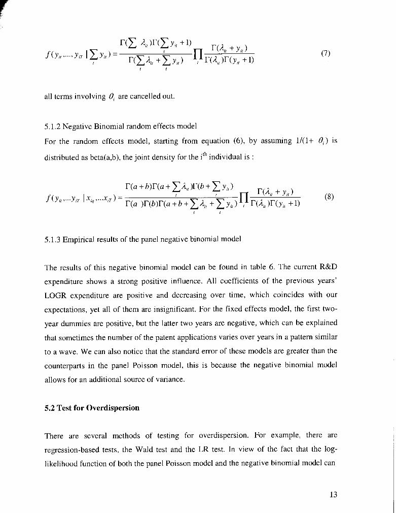
all terms involving 8, are cancelled out.
5.1.2 Negative Binomial random effects model
For the random effects model, starting from equation (6), by assuming 1/(1+ 8 , ) is
distributed as beta(a,b), the joint density for the ith individual is :
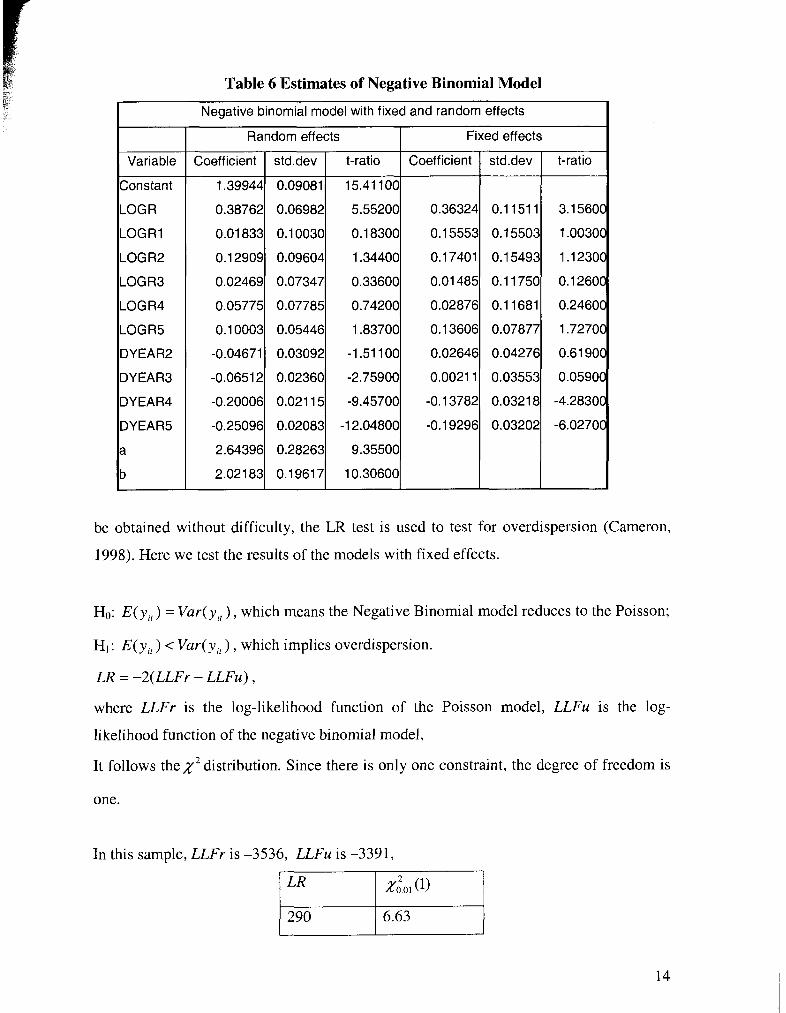
5.1.3 Empirical results of the panel negative binomial model
The results of this negative binomial model can be found in table 6. The current R&D
expenditure shows a strong positive influence. All coefficients of the previous years'
LOGR expenditure are positive and decreasing over time, which coincides with our
expectations, yet all of them are insignificant. For the fixed effects model, the first two-
year dummies are positive, but the latter two years are negative, which can be explained
that sometimes the number of the patent applications varies over years in a pattern similar
to a wave. We can also notice that the standard error of these models are greater than the
counterparts in the panel Poisson model, this is because the negative binomial model
allows for an additional source of variance.
5.2 Test for Overdispersion
There are several methods of testing for overdispersion. For example, there are
regression-based tests, the Wald test and the LR test. In view of the fact that the log-
likelihood function of both the panel Poisson model and the negative binomial model can
Table 6 Estimates of Negative Binomial Model
I Negative binomial model with fixed and random effects I
Variable
Constant
LOG R
LOGR1
LOG R2
LOGR3
LOG R4
LOGR5
DYEAR2
DYEAR3
DY EAR4
DYEAR5
a
b
Random effects
t-ratio I Coefficient I std.dev I t-ratio 1 Fixed effects
Coefficient
1.39944
0.38762
0.01 833
0.1 2909
0.02469
0.05775
0.1 0003
-0.04671
-0.0651 2
-0.20006
-0.25096
2.64396
2.02183 I l l
I std.dev
0.09081
0.06982
0.1 0030
0.09604
0.07347
0.07785
0.05446
0.03092
0.02360
0.021 15
0.02083
0.28263
0.19617
be obtained without difficulty, the LR test is used to test for overdispersion (Cameron,
1998). Here we test the results of the models with fixed effects.
Ho: E(y, ) = Var(y, ) , which means the Negative Binomial model reduces to the Poisson;
HI: E(y, ) < Var(y, ) , which implies overdispersion.
LR = -2(LLFr - LLFu) ,
where LLFr is the log-likelihood function of the Poisson model, LLFu is the log-
likelihood function of the negative binomial model,
It follows thex2 distribution. Since there is only one constraint, the degree of freedom is
one.
In this sample, LLFr is -3536, LLFu is -3391,
As one can see there is strong evidence of overdispersion, thereby the negative binomial
model is more suitable for this sample.
VI HAUSMAN TEST
Although the random effects model can include time-invariant variables and is more
efficient when compared to the fixed effects model, it is consistent only when it is
correctly specified. So it is necessary to test which one is better for our data. The
Hausman test is used on the estimates of the negative binomial model (Hausman, 1984).
Under the null hypothesis, the random effects model is correctly specified, so both the
fixed and the random effects models are consistent, while under the alternative
hypothesis, the random effects are correlated with the regressors, so the random effects
model loses its consistency.
Thus, the Hausman test:
Ho: The random effects model is appropriate. The preferred estimator is A, HI: The fixed effects model is appropriate. The preferred estimator is B , .
The Hausman test is based on the distance:
rH = (aRE - B,q )W t B, 1 - v ( B R E )I-' ( B R , - B F J
It follows that the^: distribution, with a degree of freedom of q (the dimension of P,).
From the result,
So now we can reject the null hypothesis, and accept that the fixed effects model is more
appropriate, since there is strong evidence that the firm specific effects in the random
effects model are correlated with the explanatory variables.
VII GMM ESTIMATION
GMM estimation is a very general estimation method used in econometrics. In some
sense, maximum likelihood and quasi-maximum likelihood can be considered as special
cases of GMM. The generalized method of moments (GMM) has become popular in
recent years since it requires fewer assumptions. The consistency of the estimators from
the Poisson and the Negative Binomial models in this panel count data model requires the
explanatory variables be strictly exogenous. But in the patent-R&D relationship, this
assumption is likely to fail since once a firm succeeds in one patent application, it is
likely that more R&D expenditures will be needed for full development or improvement
of products embodying the patent. Consequently R&D expenditures should not be
considered as strictly exogenous. Moreover, the GMM estimation procedure is not based
on assumptions about the distribution of the error terms. In this part of the paper, the
GMM method is applied to the fixed effects model and the results are compared to those
obtained from the previous sections2.
7.1 Introduction to GMM Method
One approach to get moment conditions for the GMM estimation is to find a set of
instrumental variables ( z, ) and residuals ( E ~ ) to satisfy the orthogonality conditions:
E[z,E,] = 0
Since E, is a function of the parameters, the estimators can be obtained by solving these
moment conditions. If the number of moment conditions (L) equals the number of
parameters (K), it is identified; if L>K, it is overidentified.
Then the sample moment conditions will be:
In case of overidentification, the GMM estimator B, will be obtained by minimizing
F = m(P)'W-'rn(fl) , where w -' is the weight matrix.
2 For a detailed introduction regarding GMM, please refer to Kennedy(2000).
7.1.1 Defining the residuals
The transformation method, developed by Chamberlain (1992), is used here to eliminate
the unobservable effects in the context of sequential moment restrictions for models with
multiplicative fixed effects. The transformation is as follows:
For the fixed effect model,
under weak exogeneity, uit
In order to eliminate the unobserved firm specific effects, rewrite (10) for t+l, and
solving for ai , then substitute back into (9), we obtain:
So vit is uncorrelated with past and current values of x.
Define:
This is the residual we are going to use.
7.1.2 Minimization criterion
Thus the GMM estimator of Pcan be obtained by minimizing
1 where \i: = - ~ ~ : i . , i . ~ ~ , , Ci is $estimated using some predetermined D .
n 1 = 1
The matrix of instruments Zi of this panel count model should look like:
where zi, is some function of the x variables.
Under mild regularity conditions, is consistent and normally distributed with the
asymptotic variance-covariance matrix:
I N where D(B) = -z .Z;VV, ( B )
N
and 0 ( B ) = w@)
7.2 Empirical Result Using GMM Estimation
In this paper, we have n=346, T=5, so the residual v, (P) is:
In order to choose the instrumental variables, we need to check the moment conditions.
The orthogonalitiy conditions of the year dummies with the residuals are same as the
moment conditions of the residual itself, so we can eliminate the redundancy. Since the
residual is uncorrelated with past and present value of the R&D expenditures, zit includes
the intercept and all previous year's LOGR. So there are 34 (7+8+9+10) moment
conditions, which are contrary to the case of strict exogeneity, where a common set of
instruments are used. Here the number of instruments increases with the number of
periods.
The estimates obtained from the negative binomial model with fixed effects are used as
the starting values. Compared with the results of the Poisson Model, the
contemporaneous R&D still has a significant effect on the patent application and the first
year's lagged R&D is no longer negative. The total effect of R&D on patents is larger
than that of the Poisson model, but not as large as the one derived from the negative
binomial model. The standard errors are also larger than that of the Poisson model,
indicating less efficiency in estimation. However, the last lag is negative and significant
and all coefficients of the year dummies are negative.
Table 7 The Result of The GMM Estimation
GMM Estimation I Variable
LOG R
LOG R 1
LOGR2
LOGR3
LOGR4
LOGR5
DY EAR2
DYEAR3
DY EAR4
DYEAR5
7.3 Overidentification Test
Another advantage of the GMM is that it provides an easy specification test for the
validity of the overidentifying restrictions. If it is exactly identified, the criterion for the
GMM estimation (F) should be zero since we can find the estimates to exactly satisfy the
moment conditions. When in the situation of overidentificaiton, the moment conditions
imply substantive restrictions. So if the model we apply to derive the moment condition
is incorrect, some of the sample moment conditions will be systematically violated.
Following Winkelmann(2000), the overidentification test:
zoefficient
0.35437
0.061 83
0.1 1762
0.08297
-0.06742
-0.1 2877
-0.02976
-0.02705
-0.1 271 2
-0.1 7532
Ho: E [ v ~ z , ] = 0 , that is the restrictions are valid.
HI: The specification is invalid.
The overidentification test is based on the minimum criterion function evaluated at
p = B and divided by the sample size, that is: F, = F l n ,
std.dev
0.1 5521
0.05830
0.05307
0.05220
0.04851
0.0461 1
0.01 372
0.01 879
0.02770
0.03572
t-ratio
2.2831 2
1.06059
2.21 61 7
1.58923
-1.38984
-2.79291
-2.1 6939
-1.43921
-4.58974
-4.90832
and the test statistic follows thex; distribution, with a degree of freedom of L-K, where
L is the number of moment conditions (34 in this case) and K is the number of parameters
(10) in this case.
So the result shows we should accept the null hypothesis that all the moment conditions
are valid at a 5% significant level.
VIII CONCLUSION
Several models were applied to study the relationship between patent applications and the
R&D expenditures. Firstly we used the Poisson model with cross-sectional data, which
overlooks the panel nature of the data and controls for heterogeneity only by including
firm specific effects such as firm size or as to whether it belongs to the science sector.
The result is then used for comparison. Then the panel Poisson models with unobservable
fixed effects and random effects are used to control for firm specific effects. One of the
assumptions of the Poisson model is that the mean and the variance should be equal,
which does not usually hold true. From the data description, we also find that the
distribution of the patent application skews to the left together with a long right tail,
which indicates that there might be overdispersion. So the alternative negative binomial
models are applied for overdispersion. Finally the GMM estimation is carried out with
the relaxed assumption of strict exogeneity, since additional R&D expenditures is very
likely to happen when the firm succeeds in a new patent.
Table 8 is the summary of estimators from different models with only time-invariant
variables. Two major results are compared. First is the coefficient of the current year's
R&D expenditure. Since P o ' s are from different generalizations of the Poisson models,
they have the same interpretation and are found to be significantly important in all the
models. The second result that is compared is the sum of all the coefficients of the current
R&D expenditure and previous years' R&D expenditures. It is approximately equal to the
product of the coefficients of R&D expenditures which is the long run effect of R&D
expenditures on patent applications. When comparing the results of different models, I
prefer the Negative Binomial model with fixed effects. According to the overdispersion
test and Hausman test, the Negative Binomial model with fixed effects is more
appropriate compared to other Poisson Models and Negative Binomial models. The result
of the estimation, that is, all coefficients of R&D expenditures are positive and the long
run effect is the highest, is in line with the assumption of the R&D-patent relationship.
Though theoretically only the estimates from the GMM estimation is consistent, it is less
efficient. The result is not very stable because of the large standard error. The only thing
we can conclude from the GMM estimation is that the contemporaneous R&D
expenditure has important effect on the number of patent applications.
Table 8 Comparison of Alternative Estimatiors
t-rati o
Model I I I I
I I I
Panel Poisson with I
Basic Poisson
Panel Poisson with fixed effects
4.3793 0.15 0.69
0.32
random effects Negative Binomial with fixed effects Negative Binomial with random effects GMM
1 1.323
0.36
0.31
0.38
0.35
3.156 0.84
5.552
2.283
0.69
0.42
APPENDIX I
Figure 1 Number of Patents Per Million R&D Expenditure
Std. Dev = 2.90
Mean = 2.9
N = 345.00
number of patents per million R&D expenditure
REFERENCES
Cameron, A.C, Trivedi, P.K. (1998), Regression analysis of count data . New York :
Cambridge University Press.
Crepon, B. and Duguet, E., "Estimating the Innovation Function From Patent Numbers:
GMM on Count Panel Data" Journal of Applied Econometrics 12(1997), 243-263.
Chamberlain, G. (1992), "Comment: Sequential Moment Restrictions in Panel Data,"
Journal of Business and Economic Statistics 10:20-26.
Greene H. William, LIMDEP User's manual and reference guide, version 7.0.
Hausman, J.A., Hall, B. H., and Griliches, Z., "Econometric Models for Count Data With
an Application to the Patents-R&D Relationship", Econometrics 52(1984), 909-938.
Hall, B. H., Griliches, Z., and Hausman, J. "Patents and R&D: Is There a Lag?"
International Economic Review 27(1986), 265-283.
Kennedy, P. (1998), A guide to econometrics. Cambridge: MIT press.
Montalvo, J.G., "GMM Estimation of Count-Panal-Data Models With Fixed Effects and
Predetermined Instruments", Journal of Business & Economic Statistics 15 (1997),
82-89.
Pakes, A., and Griliches, Z., "Patents and R&D at the Firm Level: A First Look", in
R&D, Patents and Productivity, ed. Z. Griliches, Chicago: University of Chicago
Press, (1984) pp. 55-72.
Winkelmann, R. (2000), Econometric analysis of count data. New York : Springer.