University of Calgary PRISM: University of Calgary's Digital Repository Van Horne Institute Van Horne Institute 2006-08 Analysis of the Productive Efficiency of the Urban Transport Networks in France Abbes, Souhir; Bulteau, Julie TRANSPORTATION CONFERENCE -BANFF,ALBERTA,CANADA 2006 http://hdl.handle.net/1880/44334 Presentation Downloaded from PRISM: https://prism.ucalgary.ca
Transcript
University of Calgary
PRISM: University of Calgary's Digital Repository
Van Horne Institute Van Horne Institute
2006-08
Analysis of the Productive Efficiency of the Urban
The urban transportation systems are the basis of the city-dweller's mobility. The costs of the
transportation as well as the economic activity of the agglomeration determine jointly the
performances of the system. The aim of our article is to analyze the costs of the collective
transportation networks and to determine their efficiency.
The results of our study will be useful in the evaluation of the urban transportation policies,
notably the financing politics. To our knowledge, only the collective bus network has been analyzed in
empirical studies. Viton (1981) estimates a translog cost function using a cross section database (the
sample consists of data covering 54 American cities for the year 1975). He concludes that the
collective bus network in the USA is subject to increasing returns to scale and that short run marginal
cost pricing doesn't cover the total operational cost. Finally, the production factors (fuel price and
labor) are little substitutable. The paper of Button and O'Donnell (1985) examines the cost structure of
the urban bus networks in GB in order to analyze the efficiency of the transportation firms. Cross
section data allowed them to examine the relation between the cost structure in 44 departments and the
degree of the involvement of the state (in terms of subsidy and management) in the collective
transportation. This same objective has been pursued by Hensher (1987), whose survey includes 10
transportation firms. One of them is the UTA (Urban Transit Authority), which is subsidized by the
Australian authorities. The other 9 companies are private and operate in Sydney. Finally, Raymond
and Matas (1998) estimated a translog cost function for the urban bus network in Spain. The use of
panel data allowed them to analyze the relative efficiency of every city. Their sample contains 117
observations. However, only the labor factor has been taken in account.
To reach our objective, we have specified and estimated a total cost function of the
transportation for nine French cities: Nantes, Strasbourg, Grenoble, Toulouse, Dunkerque, Dijon,
Angers, Clermont-Ferrand and Reims during the period 1997-2003. According to economic theory, we
have adopted a translogarithmic cost function. Our model contains several independent variables such
as the network length, the traffic expressed in number of traveled kilometers and the price of the labor
factor. Compared to the other empirical studies, our article has the advantage of taking into account
the price of the capital factor represented by the used equipment. Several models have been estimated
in order to find the one that explains cost structures best. Finally, a regression by OLS (Ordinary Least
Square) with dummy variables has been chosen. These variables have permitted us to capture the
heterogeneity of the cities. After comparing the cities, we have observed that Nantes network has the
lowest exploitation charges per trip. We have therefore chosen Nantes as the city of reference.
We used the Christensen and Jorgensen formula (1969) in order to determine the cost of a bus,
tram or subway, and then we made an aggregation to determine the price of the capital in every city.
The results obtained in our article permitted the analysis of efficiency and the calculation of economies
of scale and density.
3
Our article is organized as follows: in the first part, we make a survey of the literature on the
application of the cost functions and we explain the different objectives and the specifications of each.
The second part presents the database and defines the main indicators. Finally, the third part shows the
function used, the estimated econometric model and analyzes the efficiency and the economies of
scale and density.
1. APPLICATION OF THE COST FUNCTIONS IN THE COLLECTIVE URBAN
TRANSPORTATION
In the transport sector, the knowledge of the costs is essential for the decision-maker. Indeed, on
the microeconomic level, precise information concerning the costs of transportation is the basis for
decisions by public authorities. On a strategic and macroeconomic level, the global knowledge of the
costs on the scale of a region or a city enlightens the public proceedings on the choices between
transport modes (Quinet, 1998).
1.1. The different shapes of the cost functions
The approach by cost function is more global than the approach by production function
because it recognizes explicitly that the decisions concerning factor quantities used in the production
of goods are under the control of the firms1.
The hypotheses concerning the substitutability between production factors determine
extensively the different formulations of the production functions. The variable price is the
fundamental variable in the production function. The optimal combination of the factors is realized
implicitly according to their relative prices. Only the production functions with rigid coefficients2
suppose a priori (and that is their limit) the strict complementarity (ex ante and ex post) between the
different factors. The use of CES functions (Constant Elasticity of Substitution) was a first step toward
the removal of such important hypotheses. Therefore, the criteria of elasticity substitution that permits
us to distinguish between complementarity and substitutability prove to be, there again, completely
unusable. Indeed, in this case, as in the precedents, its value is imposed, which constitutes a coercive a
priori for the analysis of the substitutability of the factors. Introducing a bias in the calculations of the
substitution elasticity, the previous functions cannot answer the analysis of the transportation activity.
1 Theoretical reminder: the classic economic theory takes the case of a firm that manufactures a good in qquantity from production factors x, y and z. These variables are joined by the production function that defines the maximal quantity of q good susceptible to be produced from the factors. From there, one defines a cost function as the minimum cost of production of the quantity q.2 For example, the Cobb Douglas function, assuming a perfect substituability before and after the realization of the investments. It supposes that, whatever is the level of production and the proportion of the used factors, the elasticity of substitution is always equal to the unit and the relative part in value of the factors is always constant.
4
The estimation of a cost function implies that the firm minimizes the total cost under the
technical constraint, and supposes that factor prices are exogenous. For the collective transportation
sector in France, this hypothesis is realistic enough. Indeed, the firms cannot modify the prices of the
production factors (labor and equipment prices). In addition, the production level is exogenous, which
justifies the estimation of a cost function.
In transportation, several shapes of cost functions have been used. We can mention, for example,
the Leontief function, the Cobb-Douglas function, and the CES function. As we have just explained,
these forms put restrictions on the production technology. That's why flexible forms, defined as a
second order approximation of the true cost function (Diewert, 1974), are preferable. They are mainly
the quadratic and translogarithmic functions.
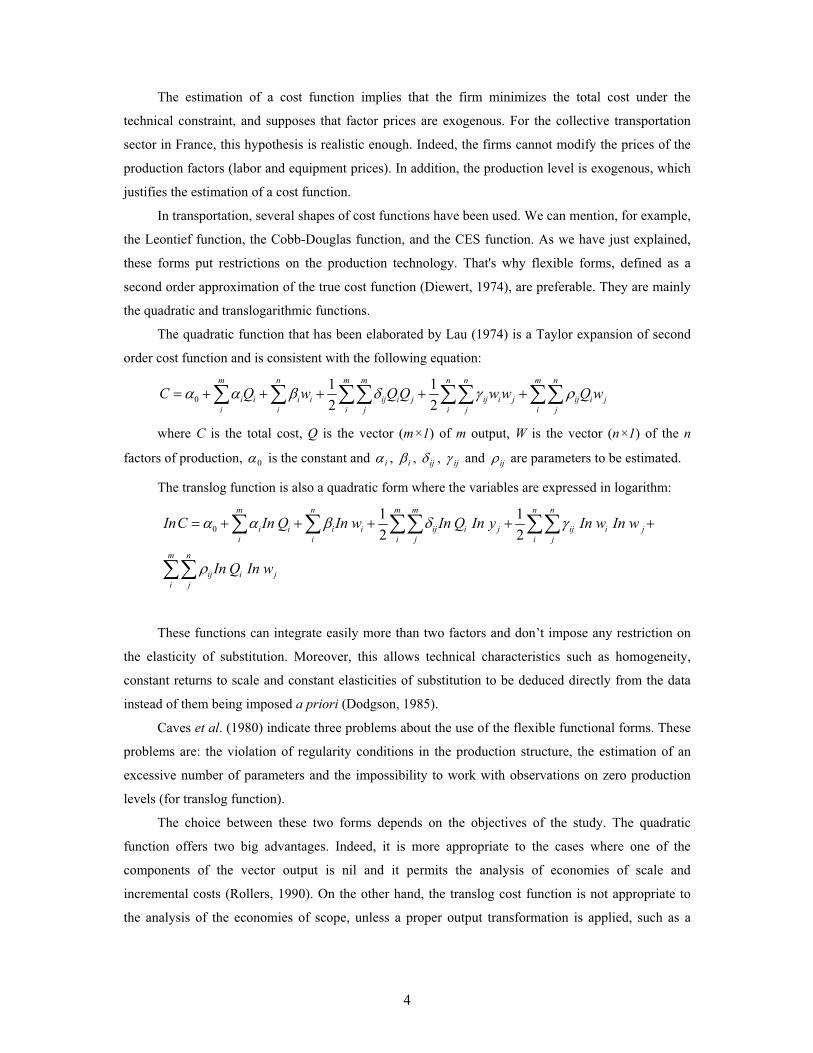
The quadratic function that has been elaborated by Lau (1974) is a Taylor expansion of second
order cost function and is consistent with the following equation:
01 12 2
m n m m n n m n
i i i i ij i j ij i j ij i ji i i j i j i j
C Q w Q Q w w Q w
where C is the total cost, Q is the vector (m×1) of m output, W is the vector (n×1) of the n
factors of production, 0 is the constant and i , i , ij , ij and ij are parameters to be estimated.
The translog function is also a quadratic form where the variables are expressed in logarithm:
01 12 2
m n m m n n
i i i i ij i j ij i ji i i j i j
m n
ij i ji j
InC In Q In w In Q In y In w In w
In Q In w
These functions can integrate easily more than two factors and don’t impose any restriction on
the elasticity of substitution. Moreover, this allows technical characteristics such as homogeneity,
constant returns to scale and constant elasticities of substitution to be deduced directly from the data
instead of them being imposed a priori (Dodgson, 1985).
Caves et al. (1980) indicate three problems about the use of the flexible functional forms. These
problems are: the violation of regularity conditions in the production structure, the estimation of an
excessive number of parameters and the impossibility to work with observations on zero production
levels (for translog function).
The choice between these two forms depends on the objectives of the study. The quadratic
function offers two big advantages. Indeed, it is more appropriate to the cases where one of the
components of the vector output is nil and it permits the analysis of economies of scale and
incremental costs (Rollers, 1990). On the other hand, the translog cost function is not appropriate to
the analysis of the economies of scope, unless a proper output transformation is applied, such as a
5
Box-Cox transformation3. Although this provides a solution, it complicates significantly the interpreta-
tion of parameters.
In contrast, the translog function’s main advantage is that it allows the analysis of the underlying
production structure, such economies of scale, the marginal cost determination ( i ) and the Hessian’s
values ( ij ) through relatively simple tests of an appropriate group of estimated parameters. On the
other hand, the number of parameters to be estimated is larger in the quadratic function than in the
translog (Caves et al., 1980), because the restraints imposed on the translog function to ensure the
conditions of homogeneity of factor prices, symmetry, etc., limiting the number of free parameters to
be estimated4.
1.2. Economic and technical features
The general shape of a cost function for an urban transportation network is the following:
( , , )CT f Q Pi N
Where Q = (Q1,…, Qn) is the vector of the output Q that can consist of one or several
components, P = (P1…, Pm), where Pi is the price of the production factor, and N the network length.
The degree of the global economies of scale is a technical property of the productive process. It
represents the maximal growth that the vector of production can reach while increasing the factors of
production. However, we can calculate the degree of the economies of scale directly through translog
cost function (Panzar and Willig, 1977) as follows:
11 ( ) ( )( )Q N
CT CTSQ N
with Q and N respectively the cost elasticity of the
output and the cost elasticity of the network length.
Another characteristic of the production technology in transport is the economies of density.
These are defined as the increase in costs that result from an increase in output while maintaining the
"network" variable unchanged. Returns to density can be seen as the inverse of the elasticity of total
costs in respect to output:
11 ( )( )Q
CTDQ
3 In this case, the problem can be solved by applying the Box-Cox transformation. In this article, we are not confronted with this problem since the collective transportation service achieves a minimum of km traveled annually. The prices of the production factors are different from zero. 4 Non-normalized quadratic function has m + n + 1 parameters more than the translog function restricted to linear homogeneity in prices.
6
1.3. Specification of the econometric model
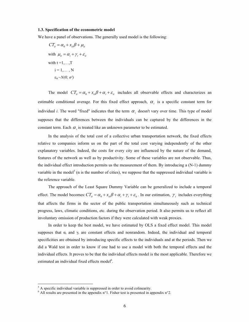
We have a panel of observations. The generally used model is the following:
0it it itCT x
with it i t it
with t =1,…,T
i = 1,… , N
it ~N(0, ²)
The model 0it it i itCT x includes all observable effects and characterizes an
estimable conditional average. For this fixed effect approach, i is a specific constant term for
individual i. The word "fixed" indicates that the term i doesn't vary over time. This type of model
supposes that the differences between the individuals can be captured by the differences in the
constant term. Each i is treated like an unknown parameter to be estimated.
In the analysis of the total cost of a collective urban transportation network, the fixed effects
relative to companies inform us on the part of the total cost varying independently of the other
explanatory variables. Indeed, the costs for every city are influenced by the nature of the demand,
features of the network as well as by productivity. Some of these variables are not observable. Thus,
the individual effect introduction permits us the measurement of them. By introducing a (N-1) dummy
variable in the model5 (n is the number of cities), we suppose that the suppressed individual variable is
the reference variable.
The approach of the Least Square Dummy Variable can be generalized to include a temporal
effect. The model becomes: 0it it i t itCT x . In our estimation, t includes everything
that affects the firms in the sector of the public transportation simultaneously such as technical
progress, laws, climatic conditions, etc. during the observation period. It also permits us to reflect all
involuntary omission of production factors if they were calculated with weak proxies.
In order to keep the best model, we have estimated by OLS a fixed effect model. This model
supposes that i and t are constant effects and nonrandom. Indeed, the individual and temporal
specificities are obtained by introducing specific effects to the individuals and at the periods. Then we
did a Wald test in order to know if one had to use a model with both the temporal effects and the
individual effects. It proves to be that the individual effects model is the most applicable. Therefore we
estimated an individual fixed effects model6.
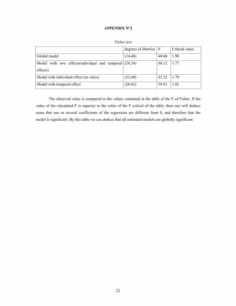
5 A specific individual variable is suppressed in order to avoid colinearity. 6 All results are presented in the appendix n°1. Fisher test is presented in appendix n°2.
7
2. THE DATABASE
2.1. Sample and measurement of the variables
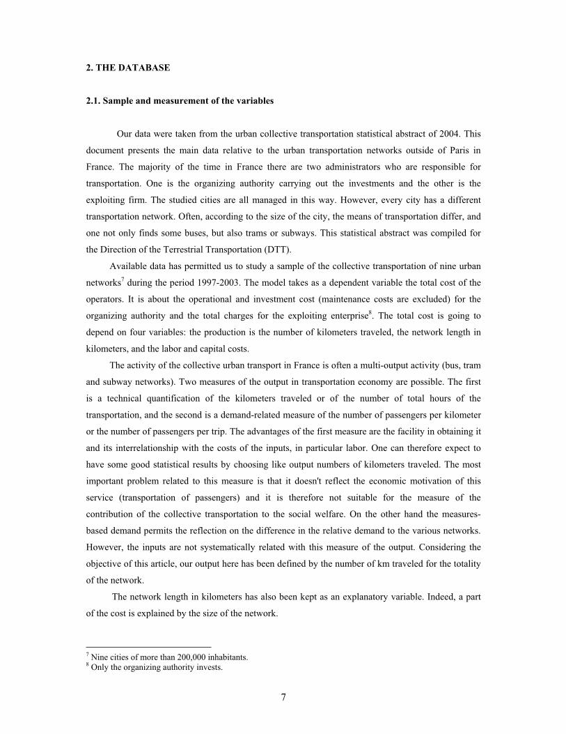
Our data were taken from the urban collective transportation statistical abstract of 2004. This
document presents the main data relative to the urban transportation networks outside of Paris in
France. The majority of the time in France there are two administrators who are responsible for
transportation. One is the organizing authority carrying out the investments and the other is the
exploiting firm. The studied cities are all managed in this way. However, every city has a different
transportation network. Often, according to the size of the city, the means of transportation differ, and
one not only finds some buses, but also trams or subways. This statistical abstract was compiled for
the Direction of the Terrestrial Transportation (DTT).
Available data has permitted us to study a sample of the collective transportation of nine urban
networks7 during the period 1997-2003. The model takes as a dependent variable the total cost of the
operators. It is about the operational and investment cost (maintenance costs are excluded) for the
organizing authority and the total charges for the exploiting enterprise8. The total cost is going to
depend on four variables: the production is the number of kilometers traveled, the network length in
kilometers, and the labor and capital costs.
The activity of the collective urban transport in France is often a multi-output activity (bus, tram
and subway networks). Two measures of the output in transportation economy are possible. The first
is a technical quantification of the kilometers traveled or of the number of total hours of the
transportation, and the second is a demand-related measure of the number of passengers per kilometer
or the number of passengers per trip. The advantages of the first measure are the facility in obtaining it
and its interrelationship with the costs of the inputs, in particular labor. One can therefore expect to
have some good statistical results by choosing like output numbers of kilometers traveled. The most
important problem related to this measure is that it doesn't reflect the economic motivation of this
service (transportation of passengers) and it is therefore not suitable for the measure of the
contribution of the collective transportation to the social welfare. On the other hand the measures-
based demand permits the reflection on the difference in the relative demand to the various networks.
However, the inputs are not systematically related with this measure of the output. Considering the
objective of this article, our output here has been defined by the number of km traveled for the totality
of the network.
The network length in kilometers has also been kept as an explanatory variable. Indeed, a part
of the cost is explained by the size of the network.
7 Nine cities of more than 200,000 inhabitants. 8 Only the organizing authority invests.
8
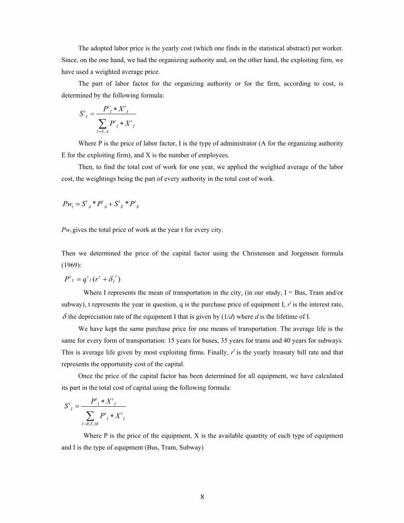
The adopted labor price is the yearly cost (which one finds in the statistical abstract) per worker.
Since, on the one hand, we had the organizing authority and, on the other hand, the exploiting firm, we
have used a weighted average price.
The part of labor factor for the organizing authority or for the firm, according to cost, is
determined by the following formula:
,
t tt I II
t tI I
I E A
P XSP X
Where P is the price of labor factor, I is the type of administrator (A for the organizing authority
E for the exploiting firm), and X is the number of employees.
Then, to find the total cost of work for one year, we applied the weighted average of the labor
cost, the weightings being the part of every authority in the total cost of work.
* *t t t tt A A E EPw S P S P
Pwt gives the total price of work at the year t for every city.
Then we determined the price of the capital factor using the Christensen and Jorgensen formula
(1969):
)( tI
tI
tI
t rqP
Where I represents the mean of transportation in the city, (in our study, I = Bus, Tram and/or
subway), t represents the year in question, q is the purchase price of equipment I, rt is the interest rate,
the depreciation rate of the equipment I that is given by (1/d) where d is the lifetime of I.
We have kept the same purchase price for one means of transportation. The average life is the
same for every form of transportation: 15 years for buses, 35 years for trams and 40 years for subways.
This is average life given by most exploiting firms. Finally, rt is the yearly treasury bill rate and that
represents the opportunity cost of the capital.
Once the price of the capital factor has been determined for all equipment, we have calculated
its part in the total cost of capital using the following formula:
, ,
t tt I II
t tI I
I B T M
P XSP X
Where P is the price of the equipment, X is the available quantity of each type of equipment
and I is the type of equipment (Bus, Tram, Subway)
9
Finally, we have produced the following aggregation in order to obtain the yearly capital price for
every city: t
MtM
tT
tT
tB
tBt PSPSPSPk ***
2.2. The main indicators
The following table shows the different indicators in the provincial transportation networks in
France. The number of trips by residents as well as the number of trips by kilometer can indicate the
frequency of the service. However, these cannot be pertinent indicators for the measure of efficiency
since they don't reflect the relation between the costs and the quantities of the factors. The number of
kilometers by driver reflects, only in part, the efficiency of the labor factor (the administrative staff of
the organizing authority is not taken into account by this indicator).
Table n°1: Average value of the main indicator between 1997 and 2003 for every city
Citiestrip by
residenttrip by km Km by driver
Exploitation
charges per
trip
Exploitation
charges per
km
Rate of
Transportation
Remittance
Nantes 149.1 4.2 21335.3 0.826 3.47 1.75%
Strasbourg 154.4 4.8 16614.6 1.016 4.75 1.75%
Reims 136.8 3.96 19115.8 1.065 4.1 1%
Dijon 144.2 3.65 21036.6 0.916 3.3 1.05%
Angers 94 2.93 23149.3 0.935 2.75 1.05%
Clermont-
Ferrand93.7 3.36 20217.8 1.026 3.41 1.6%
Dunkerque 61.7 2.53 26945.6 1.015 2.97 1%
Grenoble 132.5 4.11 16885.5 1.128 4.6 1.75%
Toulouse 175.5 4.08 19469.5 1.143 4.63 1.75%
average 126.9 3.73 20530 1.007 3.77 -
This table shows a large disparity between the networks studied. The cities that possess the most
efficient networks are Nantes, Dijon, and Angers. Indeed, these networks are located above the
average for the indicators: trips by resident, trips by kilometer and kilometer by driver. These
networks also have exploitation charges per trips and per kilometer below the average. Strasbourg,
Reims, Grenoble and Toulouse appear to be a little less efficient and Clermont-Ferrand seems to
possess the least efficient network in relation to the average of our studied networks.
10
The indicator Km by driver can reflect only the efficiency of the labor factor. Trips by Km
reflect only the frequency of the service. The exploitation charges per trip and kilometers traveled are
therefore the best indicators of the efficiency of the networks.
The Transportation Remittance (TR) is a tax whose exclusive purpose is to pay the expenses of
collective transportation. It is collected only by local collectivities organizing urban collective
transportation. The TR is owed by all firms and administrations of more than 9 employees situated in
an Urban Transportation Perimeter (PTU). The return of the TR is proportional to the salary mass. The
rate voted by the urban transportation organizing authorities cannot pass a percent fixed by the
government. This figure varies from 0.55% to 1.75%, according to the size of the PTU. The TR is a
contribution by the employers to the efforts made by the township to facilitate residence-work
displacements. For the cities of more than 100,000 residents, the TR represents 52% of the sources of
the financing of the urban collective transportation out of Paris. It is the most important source of
financing in urban transportation network (see graphic in appendix n°3).
3. ESTIMATION OF THE ECONOMETRIC MODEL
3.1. The shape of the function
We have estimated several econometric models by the OLS. It is about translog cost functions
explained by the Q output, the prices of labor and capital factor (respectively W and K) and N the
network length. After having estimated several models, we used the Hausman (1978) test in order to
choose between a model with fixed effects and a model with random effects. The model with fixed
effects cities has been kept.
The econometric specification of the model with city effects is the following:
01 1 1ln ln (ln )² ln (ln )² ln (ln )²2 2 2
1ln (ln )² ln *ln ln *ln ln *ln ln *ln2
ln *ln ln *ln
i q qq w ww k kk
n nn qw qk qn wk
wn kn it
CT Q Q W W K K
N N Q W Q K Q N W K
W N K N
This is a translog cost function where CT is total operational cost, Q is kilometers traveled, W is
the price of the labor factor, K is the price of the capital factor, i is specific effects of every city and
it is a random term.
We have chosen as an efficiency indicator the exploitation charges per trip. Nantes appears to
be the most efficient city, which means that the coefficients found for the other cities will be compared
11
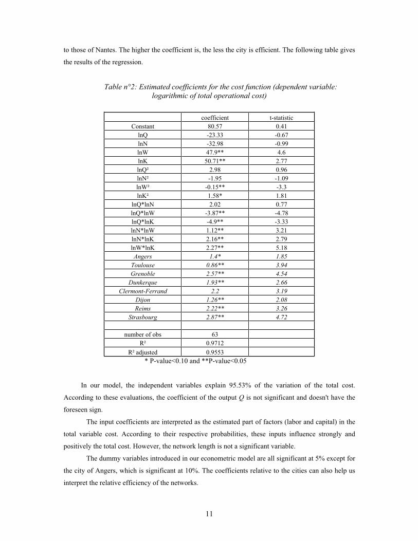
to those of Nantes. The higher the coefficient is, the less the city is efficient. The following table gives
the results of the regression.
Table n°2: Estimated coefficients for the cost function (dependent variable: logarithmic of total operational cost)
According to this table, we can deduce two assumptions.
- First, the financial aid paid to the exploiting firm doesn't influence its efficiency.
13
- Second, this rate influences efficiency. However, in Grenoble and Strasbourg, this aid is
reflected more in the fixed costs. It has been confirmed by several empiric works9 that concluded that
the subsidies generally entail the increase of costs, which is the source of the inefficiency of the
transportation network.
The exploiting firms work collaboration with the organizing authority has produced different
types of contracts (inclusive financial Contribution, Concession, Management or Management to
inclusive price). For the cities of Nantes, Toulouse, Angers, Dunkerque and Clermont-Ferrand, the
length of the contract varies between 5 and 7 years. On the other hand, it rises to 10 years for Reims
and 30 years for Grenoble and Strasbourg. These contracts of such long length often give to the
exploiting firm the status of a local monopoly, which doesn't encourage the reduction of the costs
especially since they benefit from an elevated rate of remittance transportation.
We have also noticed that the ordering of these cities has a relation to the size of the network
with the exception of Grenoble and Strasbourg. We then revalued the model while suppressing the
variable length of the network in order to get the corrected fixed effects. According to the new
ordering, there is not a clear interrelationship between the rate of RT and the efficiency of the network.
However, one notices that Grenoble and Strasbourg remain among the least efficient cities.
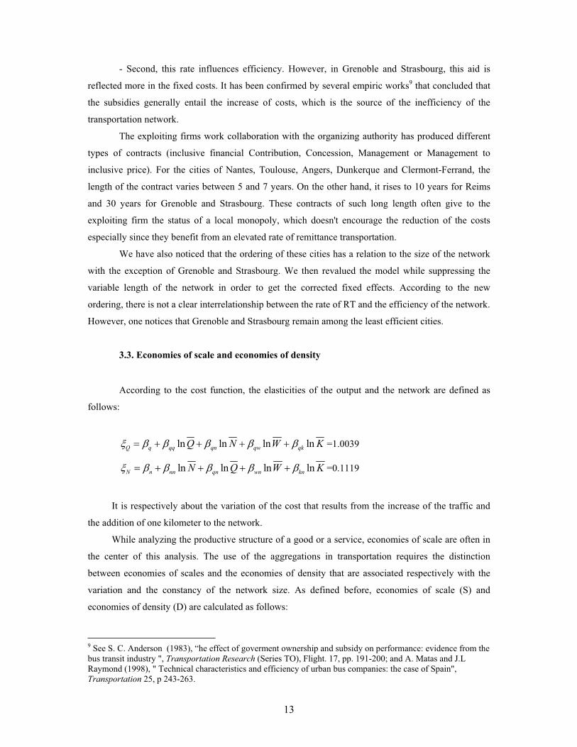
3.3. Economies of scale and economies of density
According to the cost function, the elasticities of the output and the network are defined as
follows:
ln ln ln lnQ q qq qn qw qkQ N W K =1.0039
ln ln ln lnN n nn qn wn knN Q W K =0.1119
It is respectively about the variation of the cost that results from the increase of the traffic and
the addition of one kilometer to the network.
While analyzing the productive structure of a good or a service, economies of scale are often in
the center of this analysis. The use of the aggregations in transportation requires the distinction
between economies of scales and the economies of density that are associated respectively with the
variation and the constancy of the network size. As defined before, economies of scale (S) and
economies of density (D) are calculated as follows:
9 See S. C. Anderson (1983), “he effect of goverment ownership and subsidy on performance: evidence from the bus transit industry ", Transportation Research (Series TO), Flight. 17, pp. 191-200; and A. Matas and J.L Raymond (1998), " Technical characteristics and efficiency of urban bus companies: the case of Spain", Transportation 25, p 243-263.
14
1
Q N
S and 1
Q
D
Considering the positivity of the elasticity of N (which has been proven by most econometric
studies), one generally has S <D.
According to Oum and Waters (1996, p 429), the outputs of density reflect the impact of the
increase of traffic on the average cost to constant size of the network. Economies of scale reflect the
impact of a proportional and equivalent increase of traffic and the size of the network on the average
costs. Thus, in collective transportation, the increasing outputs of scale (S>1) suggest that the traffic
and the size of the network should be increased because the servicing of a larger network has made the
average cost lower. The outputs of constant scale with increasing outputs of density (D>1) imply that
the traffic must increase while maintaining the size of the network constant. According to the previous
definitions, economies of scale and density (calculated to the average of the sample) are the following:
S = 0.8969, D=0.9961,
According to these results, one can note that the network of urban collective transportation in
France is subject to weak diseconomies of scale and to economies of density nearly constant. This
means that to a variable network size, all increase in the traffic entails a slightly higher increase cost,
whereas with size of network constant, the increase in traffic entails a proportional increase in costs.
According to the point of view of the transportation policy, one can conclude that for the French
network, in general, it is preferable to keep constant the size of the network if the traffic must be
increased.
The convention in the econometric studies is to use the sample average to calculate the different
costs (average and marginal) and economies of scale and density. However, this average is often
influenced by the extreme values of the observations, in particular if the sample is heterogeneous
enough, which is the case of our database. An alternative approach would therefore be calculating
economies of scales and density for every city. However, we can evoke two limits to this. The first one
is that the estimated coefficients of the cost function represent no city (it is about relative coefficients
to the set of the network). The second one is that the calculation of a level of output for every city
gives a local measure of economies of scales and therefore cannot be theoretically generalized for
measures (or interpretations) in the long term. While calculating the outputs of density and scale for
every city, we obtained the following results:
15
Table 4: Economies of scale and density:
Rate of remittance
transportationof %
Length of the network on
average
Economies of
scale
Economies of
density
Nantes 1.75 690 0.873 1.018
Toulouse 1.75 697 0.886 1.097
Dijon 1 320.16 0.864 0.881
Angers 1.05 431.6 0.877 0.862
Dunkerque 1.05 225.67 0.979 0.977
Clermont-Ferrand 1.6 236 0.894 0.942
Reims 1 177.83 0.902 0.972
Grenoble 1.75 340.66 0.904 1.16
Strasbourg 1.75 329.33 0.898 1.131
According to these results, we notice that the economies of density are increasing for the cities
of Grenoble and Strasbourg and are constant for Nantes and Toulouse. For the first two cities, it means
that an increase of the output entails a less proportional increase in costs. A reduction of the unit cost
can therefore be considered by an increase in the density (more destination points served) of the
networks (bus, tram and/or subway) in these cities rather than an increase in the size of the network.
The increase in density will permit a better use of resources and an increase in productivity. For
Nantes and Toulouse, we can say that the density of the network is nearly optimal (D~1). Again we
think, that financial aid has a relation to the results in these cities. Indeed, it can happen that a more
elevated remittance rate has permitted a higher density of the network in relation to the other cities.
With regard to economies of scale, we obtain the same results (weak diseconomies) as in the
generalized case of the network, although that comes closer to the unit for some cities. We notice that
the least extended networks have the most elevated scale economies (Dunkerque, Reims, Clermont-
Ferrand). This is coherent enough with economic literature, since the more business increases the
lower the costs. In our survey, we can notice that if the size of the network surpasses a certain size (say
beyond 400 kilometers), the diseconomies of scale are higher (one can also say that the economies of
scales are lower) and the costs in this phase are increased (Nantes, Toulouse and Angers). In most
empirical studies, we obtain the same result except for the increasing economies of scale at the start10.
It confirms the traditional U shape of the average cost curve. Therefore beyond a certain size of the
network, it is preferable that the big enterprises (in particular Toulouse that has a very elevated
10 See Viton for example (1981) and Of Rus and Nombela (1997)
16
average cost) are subdivided into small firms that can serve every segment of the market separately
(tram, subway and/or bus) in order to improve productivity through the encouragement to competitive-
ness.
The following diagram representing the evolution of the average cost with the network size (the
different rates of remittance are taken next to the different corresponding points) confirms our
findings. Indeed, one can easily see that for the two choices that correspond to very elevated average
costs (the cities of Strasbourg and Grenoble), the rate of remittance is equal to 1.75 which means that
in these exploiting firms, an elevated RT doesn't help to produce in an efficient way (results confirmed
by the results of the efficiency analysis).
Graphic 1: Average cost, size of the network and rate of remittance
The interpretation of the report between marginal cost and pricing is complex enough here since
the marginal cost is interpreted as the cost of one supplementary kilometer whereas the tariff is
generally applied according to the time of trip. In order to be able to make some comparisons, the best
is to estimate a cost function that depends on the time where the output is explained by the demand of
trips or by the number of hours traveled.
17
CONCLUSION
This empirical survey analyzes the efficiency of the collective urban transportation network in
France, as well as some technical features of the production process of this service. A translogarithmic
cost function has been estimated using panel data that regroup nine cities of more than 200,000
residents during the period 1997-2003. The analysis of the relative efficiency showed that the most
efficient cities of the network are Nantes and Toulouse. The least efficient cities are Grenoble and
Strasbourg. Since these four cities have the same rate of remittance from the organizing authority, it
led us to develop two different conclusions. The first one is that the rate of remittance has no relation
to the efficiency of the city. This conclusion has been confirmed by the calculation of the corrected
individual effects. The second conclusion is that in the cities of Grenoble and Strasbourg, a more
elevated remittance rate is reflected in part by an increase in fixed costs, hence their inefficiency. This
has been demonstrated by several empirical studies for other transportation networks. In addition, we
have noted that the exploiting enterprises in these two cities (Grenoble and Strasbourg) detain a local
monopoly due to their contracts of exploitation whose length continues for 30 years, which can
explain in part their weak efficiency.
The evaluation of economies of scale and density in the network of transportation in France
has showed that there are weak slight diseconomies of scale and a density of the network nearly
constant: if the traffic must be increased, it will then be necessary to keep the size of the network
constant. In Grenoble and Strasbourg, returns of density are increasing, which means that in these two
cities, it will be possible to lower the unit cost through an increase in density. According to the average
cost curve, one can see that it is rather high for these two cities that benefit at the same time from an
elevated remittance rate. This confirms the second conclusion that we obtained through the efficiency
analysis.
Even though this article takes into account the capital factor represented by the used
equipment, it reveals some limits. On the one hand, the evaluation of a uni-product cost function
hasn’t permitted the study of every transportation network in a detailed way. An estimation of a multi-
product cost function could have permitted us to calculate efficiency and economies of scale for every
means of transportation. The calculations that we have made permit us to know if it is preferable or
not for a city to specialize in the offer of a service (bus, tram or subway) rather than to offer a
combination of these services. On the other hand, the choice of our efficiency indicator can also be a
source of bias in our evaluation.
18
BIBLIOGRAPHY
Bairam E.I., (1998), Production and cost functions: specification, measurement and applications,
Ashgate, United Kingdom.
Baumol, W., Panzar, J. and Willig, R. (1982), Contestable markets and the theory of industry
Structure. New York, Harcourt, Bruce and Jovandich, Inc.
Button K.J et O'Donnell K.J (1985), "An examination of the cost structures associated with providing
urban bus services in Britain", South Journal of Political Economy, Vol 32, No 1, p 67-81.
Caves, W., Christensen, L. R. and Tretheway, M. W. (1980), "Flexible cost functions for multiproduct
firms". The Review of Economics and Statistics. Nº 62, pp. 477-481.
Christensen, R. and Jorgenson, D. W (1969), "The measurement of U.S. real capital input, 1929-
1967". The Review of Income and Wealth. Vol. 5, pp. 293-320.
De Rus G and Nombela G (1997), "Privatisation of Urban Bus Services in Spain". Journal of
Transport Economics and Policy 31(1): 115–129.
Diewert, W. E. (1974), "Applications of duality theory". In M.D. and D.A. Kendnick. Frontiers of
Quantitative Economics. Vol. II, Amsterdam: North-Holland, pp. 106-171.
Dodgson, J.S. (1985): "A survey of recent developments in the measurement of rail total factor
productivity". In Button, K.J. and Pitfield, D. (Eds.), International Railway Economics. Gower,
Aldershot, pp. 13-48.
Fandel, G. (1991), Theory of production and cost, New York.