Evaluating the Productive Efficiency and Performance of U ...

Evaluating the Productive Efficiency and Performanceof U.S. Commercial BanksHH

Richard S. BarrSouthern Methodist University

Kory A. KillgoFederal Reserve Bank of Dallas

Thomas F. Siems*

Federal Reserve Bank of Dallas

and

Sheri ZimmelSouthern Methodist University

December 1999

Abstract: In this study, we use a constrained multiplier, input-oriented, data envelopmentanalysis (DEA) model to evaluate the productive efficiency and performance of U.S.commercial banks from 1984 to 1998. We find strong and consistent relationshipsbetween efficiency and our inputs and outputs, as well as independent measures of bankperformance. Further, our results suggest that the impact of varying economic conditionsis mediated to some extent by the relative efficiencies of the banks that operate in theseconditions. Finally, we find a close relationship exists between efficiency and soundnessas determined by bank examiner ratings.

JEL Classification: C60, D24, G21, L2

Keywords: Banks; Efficiency; Performance; Benchmarking; Data envelopment analysis

H The views expressed in this paper do not necessarily represent those of the Federal Reserve Bank ofDallas or the Federal Reserve System. This research was supported in part by the National ScienceFoundation, grant DMII 93-13346, and the Texas Higher Education Coordinating Board, AdvancedTechnology Program, grant ATP-003613-023.

* Corresponding author. Federal Reserve Bank of Dallas, Research Department, 2200 N. Pearl St., Dallas,Texas, 75201; telephone: 214-922-5129; fax: 214-922-5351; email: [email protected].

1

1. Introduction

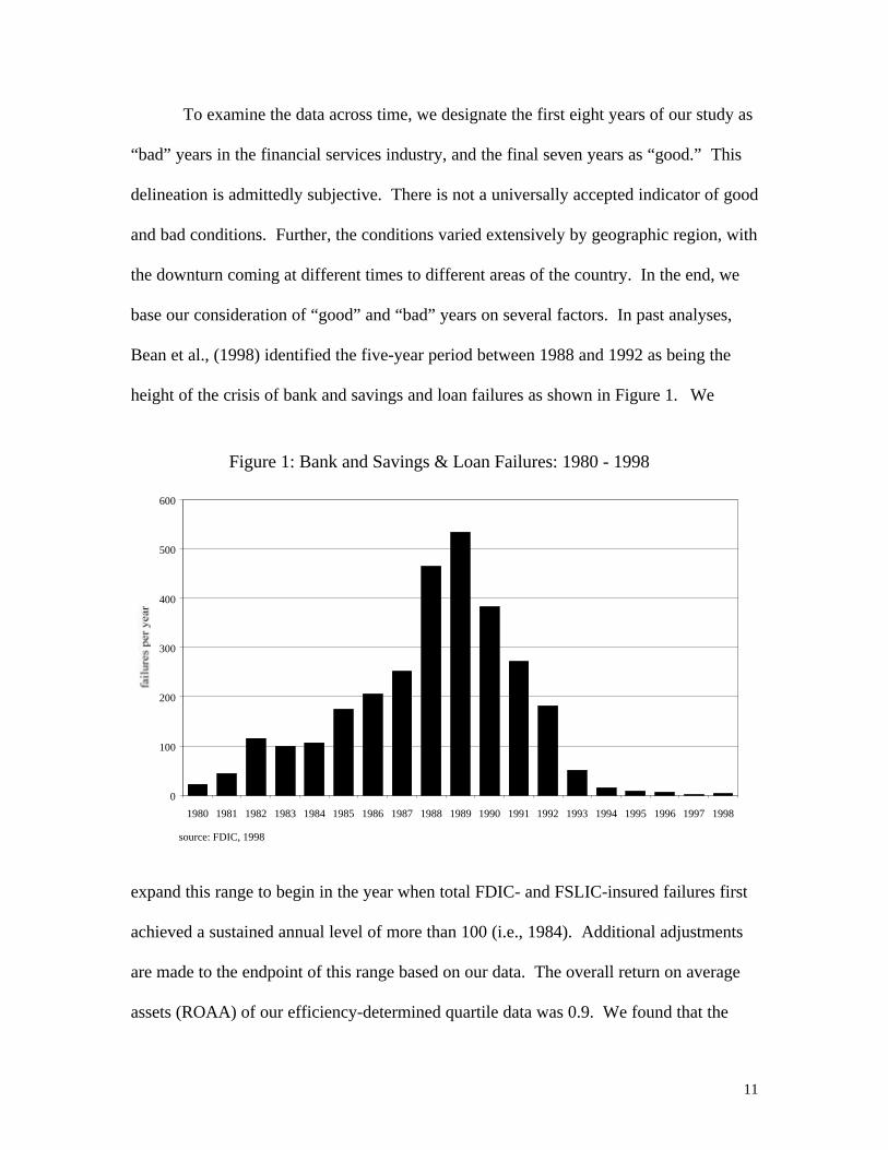
Over the past two decades, substantial research by financial economists in

government and academia from all over the world has gone into evaluating the

efficiencies of financial institutions. Berger and Humphrey (1997) survey 130 studies

that apply frontier efficiency analysis to financial institutions in 21 countries. The vast

majority of these studies were published in the 1990s, highlighting the importance and

greater frequency of this research in recent years.

Not coincidentally, this research and literature has expanded and evolved at a time

of great change in world financial markets. A number of forces have fundamentally

changed the world in which financial services providers compete, including technology,

regulations, and economic changes. For U.S. commercial banks, recent years have

witnessed sweeping changes in the regulatory environment, huge growth in off-balance

sheet risk management financial instruments, the introduction of e-commerce and on-line

banking, and significant financial industry consolidation. All of these forces have made

the U.S. banking industry highly competitive.

In competitive industries, production units can be separated by some standard into

those that perform relatively well and those that perform relatively poorly. Financial

economists have done this “separation” by applying nonparametric and parametric

frontier efficiency analyses. Berger and Humphrey explain that information obtained

from such studies can be used for a variety of reasons. They can inform government

policy by assessing the effects of various regulatory changes on efficiency. Research

issues can be addressed by describing the efficiency of an industry. Additionally,

2

managerial performance can be improved by identifying “best practices” and “worst

practices” associated with high and low efficiency, respectively.

Success in competitive markets demands achieving the highest levels of

performance through continuous improvement and learning. Comparative analyses and

benchmarking information can alert institutions to new paradigms and new practices,

leading to significant increases in firm efficiency and effectiveness. Frontier analysis

methodologies are essentially sophisticated ways to benchmark institutions to determine

the relative performance or efficiency among competing firms. Such analyses can

identify best practice institutions and provide a numerical efficiency score and ranking

for each institution that can be useful to policymakers, industry analysts, and

management of competing firms.

In this paper, we use a constrained-multiplier, input-oriented data envelopment

analysis (DEA) model to quantifiably benchmark the productive efficiency of U.S.

commercial banks. Using the parsimonious DEA model developed by Siems and Barr

(1998), we measure relative productive efficiency of these institutions over the 15-year

period from 1984 to 1998. We find strong and consistent relationships between

efficiency and our inputs and outputs, as well as independent measures of bank

performance. Further, our results suggest that the impact of varying economic conditions

is mediated to some extent by the relative efficiencies of the banks that operate in these

conditions. Finally, we find a close relationship exists between efficiency and soundness

as determined by bank examiner ratings.

3

2. The efficiency of financial institutions

The financial institution efficiency literature is now both large and recent. Berger

and Humphrey (1997) report that of the 130 studies that apply frontier analysis to

determine financial institution efficiency, 116 were published from 1992 to 1997. Berger

and Humphrey also report that there are now enough frontier analysis studies to draw

some tentative comparisons of average efficiency levels both across measurement

techniques and across countries, as well as outline the primary results of the many

applications of efficiency analysis to policy and research issues. They find that overall,

depository financial institutions�banks, savings and loans, and credit

unions�experience annual average technical efficiency ratios of around 77 percent

(median 82 percent).1 Frontier inefficiency, sometimes called X-inefficiency, at

financial institutions has generally been found to consume a considerable portion of

costs, to be a much greater source of performance problems than either scale or product

mix inefficiencies, and to have a strong empirical association with higher probabilities of

failures (see Bauer et al., 1998).

Previous studies have examined efficiency and associated effects on financial

institution performance from several different perspectives. These include the effects of

mergers and acquisitions (see Berger, Demsetz, and Strahan, 1999, and Resti, 1998),

institution failure (see Barr, Seiford, and Siems, 1993, and Cebenoyan, Cooperman, and

Register, 1993), and deregulation issues (see Humphrey and Pulley, 1997, and DeYoung,

1998), among many others. Frontier efficiency models are employed by these

researchers over other performance indicators primarily because these models result in an

1 A 77 percent efficiency measure typically means that if the average firm were producing on the frontier instead of at its currentlocation, then only 77 percent of the resources currently being used would be necessary to produce the same output (or meet the sameobjectives).

4

objectively determined quantified measure of relative performance that removes the

effects of many exogenous factors. This permits the researcher to focus on quantified

measures of costs, inputs, outputs, revenues, profits, etc. to impute efficiency relative to

the best practice institutions in the population.

There are at least four frontier analysis methodologies used to compute financial

institution efficiency, and there is no consensus among researchers on which method is

best. The approaches differ mainly in how they handle random error and their

assumptions regarding the shape of the efficient frontier. The three main parametric

methodologies include the stochastic frontier approach (SFA), the thick frontier approach

(TFA), and the distribution-free approach (DFA). In general, parametric approaches

specify a functional form for the cost, profit, or production relationship among inputs,

outputs, and environmental factors, and allow for random error. The main nonparametric

approach is data envelopment analysis. Originally developed by Charnes, Cooper, and

Rhodes (1978), DEA computes the relative technical (or productive) efficiency of

individual decision-making units by using multiple inputs and multiple outputs.

DEA has proven to be a valuable tool for strategic, policy, and operational

problems, particularly in the service and nonprofit sectors. Its usefulness to

benchmarking is adapted here to provide an analytical, quantitative benchmarking tool

for measuring relative productive efficiency. That is, DEA generally focuses on

technological, or productive, efficiency rather than economic efficiency.

Productive efficiency examines levels of inputs relative to levels of outputs. To

be productively efficient, a firm must either maximize its outputs given its input

quantities, or minimize its inputs given outputs. Economic efficiency is somewhat

5

broader in that it involves optimally choosing the levels and mixes of inputs and/or

outputs based on reactions to market prices. To be economically efficient, a firm seeks to

optimize some economic goal, such as cost minimization or profit maximization. In this

sense, economic efficiency requires both productive efficiency and allocative efficiency.

As discussed in Bauer et al. (1998), it is quite plausible that some productively

efficient firms are economically inefficient, and vice versa. Such efficiency mismatches

depend on the relationship between managers’ abilities to utilize the best technologies

and their abilities to respond to market signals. Productive efficiency requires only input

and output data, whereas economic efficiency also requires market price data. Allocative

efficiency is about doing things right, and economic efficiency is about doing the right

things right. DEA was developed specifically to measure relative productive efficiency,

which is our focus here.

3. Mathematical foundations for DEA

DEA generalizes the Farrell (1957) single-output/single-input technical efficiency

measure to the multiple-output/multiple-input case. DEA optimizes on each individual

observation with the objective of calculating a discrete piecewise linear frontier

determined by the set of Pareto-efficient decision making units (DMUs). Using this

frontier, DEA computes a maximal performance measure for each DMU relative to all

other DMUs. The only restriction is that each DMU lie on the efficient (extremal)

frontier or be enveloped within the frontier. The DMUs that lie on the frontier are the

best practice institutions and retain a value of one; those enveloped by the extremal

6

surface are scaled against a convex combination of the DMUs on the frontier facet closest

to it and have values somewhere between 0 and 1.

Several different mathematical programming DEA models have been proposed in

the literature (see Charnes et al., 1994). Essentially, these various models each seek to

establish which of n DMUs determine the envelopment surface, or best practice

efficiency frontier. The geometry of this envelopment surface is prescribed by the

specific DEA model employed.

To guide this discussion, first assume that there are n banks to be evaluated. Each

bank utilizes varying amounts of m different inputs to produce s different outputs.

Specifically, bank j uses amounts Xj = {xij} of inputs i = 1,...,m and produces amounts Yj

= {yrj} of outputs r = 1,...,s. We assume that the observed values are positive, so that xij >

0 and yrj > 0. The s · n matrix of output measures is denoted by Y and the m · n matrix of

input measures is denoted by X.

We use a constrained-multiplier, CCR input-oriented DEA model to reduce the

multiple-input, multiple-output situation for each bank to a scalar measure of efficiency

(see Charnes, Cooper, and Rhodes, 1978). Consider the following ratio form of the

model:

max EFFk = (3urkyrk)/( 3vikxik)

subject to: (3urkyrj)/( 3vikxij) # 1; j=1,...,n. (1)

3urk > 0; r=1,...,s.

3vik > 0; i=1,...,m.

0 > 0.

7

This model evaluates the relative efficiency of bank k based on the performance

of j=1,...,n banks in the population, where the yrj and xij variables in the model represent

the observed amounts of the rth output and the ith input, respectively, of the jth bank.

Thus, the multiple-input/multiple-output ratio being maximized in the objective function

provides a measure of relative productive efficiency that is a function of the multipliers.

The multipliers are the unit weights for each of the outputs and inputs, designated by urk

and vik, respectively. These are the decision variables in the model, so that the objective

function seeks to maximize the ratio of the total weighted output of bank k divided by its

total weighted input. For the constrained multiplier model, these weights must be within

an established range specified by the analyst. The 0 > 0 in the model represents a non-

Archimedean constant that is smaller than any positive-valued real number.

Each bank’s maximum efficiency score will be less than or equal to 1 by virtue of

the constraints. A value of EFFk = 1 represents full efficiency and it follows that bank k

is a “best practice” bank. When EFFk < 1, then some level of inefficiency is present.

These efficiency values provide not only a way to benchmark productive efficiency, but

also make it possible to identify the sources and amounts of inefficiency in each input

and output for every unit being evaluated (see Bowlin, 1998).

The fractional linear programming problem presented above can be transformed

into an equivalent ordinary linear programming problem following Charnes and Cooper

(1962). The results of this transformation, which are described in Charnes, Cooper, and

Rhodes (1978) results in the following linear programming problem:

max EFFk = 3urkyrk

subject to: 3urkyrj – 3vikxij # 0 (2)

8

3vikxik = 1

-urk # -0

-vik # -0

This formulation, while equivalent to the fractional problem presented earlier, can

be interpreted as maximizing the sum of the weighted outputs (virtual output) for bank k

subject to unit virtual input for bank k while maintaining the condition that virtual output

cannot exceed virtual input for any bank. Charnes et al. (1985) note that this implies the

conditions for Pareto optimality. That is, further increases in this value can be attained

only if some of the xij inputs are increased or if some of the yrj outputs are decreased.

4. Data and model specification

We use year-end data for U.S. commercial banks from 1984 to 1998. To evaluate

productive efficiency, we incorporate the constrained-multiplier, input-oriented DEA

model described in Siems and Barr (1998). This five-input, three-output model captures

the essential financial intermediation functions of a bank and uses variables employed in

similar studies (see Berger and Mester, 1997). Essentially, the model approximates the

bank management decision-making process by incorporating the necessary input

allocation and product mix decisions needed to attract deposits and make favorable loans

and investments.

The five inputs generally represent resources required to operate a bank: salary

expense, premises and fixed assets, other noninterest expense, interest expense, and

purchased funds (which are large dollar deposits). The three outputs primarily represent

9

desired outcomes: earning assets, interest income, and noninterest income. Greater detail

on the variable definitions is given in Table 1.

Using this model, banks allocate resources and control internal processes by

effectively managing their employees, facilities, expenses, and sources and uses of funds

while working to maximize earning assets and total income. Banks that do this best (the

best practice banks) are on the efficient frontier. Banks with too much input or too little

output relative to some subset of their peers, are productively inefficient to some extent.

As stated earlier, we employ a constrained-multiplier model which requires that

the weights (the urk’s and vik’s) be within some prescribed range. These upper and lower

bounds were determined through a survey of experienced bank examiners regarding their

knowledge of factors that are important in judging bank management quality.2 The

survey was intended to identify the correct set of the most important inputs and outputs,

and then evaluate the importance of each variable in relation to the others. Examiners

were asked “Which of the given list of criteria are most important in judging and

influencing the quality of bank management?”

The “given list of criteria” referenced the five inputs and three outputs used in our

model. Table 2 shows the upper and lower bounds on the values of the multipliers that

were established from the survey based on an average of the relative scores given by the

bank examiners. As shown, four of the five publicly available input variables used in our

model have relatively equal importance; only premises/fixed assets has a much lower

average weight range. For the three publicly available output variables, earning assets is

clearly the most important, followed by interest income and then noninterest income.

2 This survey was administered to twelve senior bank examiners at the Federal Reserve Bank of Dallas.

10

5. Hypotheses

Our overall hypothesis in this study is that more efficient institutions differ

significantly from less efficient institutions (as determined by our DEA model) in

measurable ways, and these results can be used for benchmarking. As one would expect,

some measurable differences should manifest themselves particularly in the DEA

model’s inputs and outputs. But we also expect to see differences in a variety of bank

performance measures and between strong and weak institutions as determined by bank

examiner ratings. Specifically, we anticipate that the differences between more efficient

institutions and less efficient institutions would tend to be those summarized in Table 3.

That is, for the inputs and outputs utilized in our model, we expect that more efficient

institutions should tend to have lower expenses, fixed assets, purchased funds,

nonperforming loans, and loans-to-assets. More efficient institutions should also tend to

have higher income, earning assets, and return on average assets. Further, more efficient

institutions should be stronger institutions as determined by bank examiner ratings.

An added benefit of the sequential nature of our data is to enable a rudimentary

longitudinal analysis of efficiency using these inputs, outputs, and related measures. The

15-year range of our data (1984-1998) subsumes periods that were both profitable and

difficult for financial institutions in the United States. We are also interested to see if

these changing conditions have different impacts on the performance measures of

institutions of varying efficiencies. Our overall hypothesis in this regard is that more

difficult banking conditions would tend to exacerbate the differences between more and

less efficient institutions, while improved conditions would close the gap between

efficiency levels.

11

To examine the data across time, we designate the first eight years of our study as

“bad” years in the financial services industry, and the final seven years as “good.” This

delineation is admittedly subjective. There is not a universally accepted indicator of good

and bad conditions. Further, the conditions varied extensively by geographic region, with

the downturn coming at different times to different areas of the country. In the end, we

base our consideration of “good” and “bad” years on several factors. In past analyses,

Bean et al., (1998) identified the five-year period between 1988 and 1992 as being the

height of the crisis of bank and savings and loan failures as shown in Figure 1. We

expand this range to begin in the year when total FDIC- and FSLIC-insured failures first

achieved a sustained annual level of more than 100 (i.e., 1984). Additional adjustments

are made to the endpoint of this range based on our data. The overall return on average

assets (ROAA) of our efficiency-determined quartile data was 0.9. We found that the

Figure 1: Bank and Savings & Loan Failures: 1980 - 1998

0

100

200

300

400

500

600

1980 1981 1982 1983 1984 1985 1986 1987 1988 1989 1990 1991 1992 1993 1994 1995 1996 1997 1998

source: FDIC, 1998

12

average ROAA in each of the years from 1984-1991 was less than 0.9, and that the

average in each of the years from 1992-1998 was greater than 0.9. We therefore use

1991-1992 as the arbitrary but functional “bad-to-good” turning point. The use of these

ranges has the added benefit of bisecting our data into groups of similar size.

6. Model results

Our DEA model was applied to publicly available year-end data reported by U.S.

commercial banks from 1984 through 1998. This 15-year range witnessed a wide variety

of economic climates, in which the banking industry experienced both difficult and

profitable periods. For the purposes of our analysis, de novo institutions (defined as those

institutions that were less than three years old) are not included, as such institutions tend

to have cost structures that differ significantly from more established institutions (see

DeYoung, 1998). Also excluded are banks that reported nonpositive values for any of the

input or output measures,3 as such values are frequently indicative of reporting error or

anomalous operation.

To isolate the relative input and output characteristics of banks for further

analysis, the banks that met our criteria are separated into quartiles by their derived

efficiency score. These four groups serve as the basis for our comparison of more and

less efficient banks vis-à-vis the DEA models’ individual inputs (salary expense, fixed

assets, other noninterest expense, interest expense, purchased funds) and outputs (earning

assets, interest income and noninterest income). To control for banks of varying sizes,

we employ a weighted ratio for each of the eight components using the appropriate asset

3 The exception to this rule was to include institutions with a zero value for purchased funds, which is not uncommon.

13

measure: quarter-end assets for balance sheet-related items (fixed assets, purchased funds

and earning assets) and average assets for the remaining income and expense-related

items. Additionally, we analyze the four groups of institutions using three general

measures of bank performance: return on average assets, the ratio of nonperforming loans

to gross loans, and the ratio of gross loans to total assets.

An important concern at the outset of this study was to evaluate the reliability of

the DEA model over time, i.e., does the efficiency score perform as a consistent measure?

A t-test of the scores reveals that in each year of the study the differences between means

of the most efficient group and the least efficient group are significant at the 0.01 level,

suggesting a level of differentiation that permits us to regard differences between the

efficiency-ranked quartiles as meaningful. As shown in Figure 2, this level of statistical

significance is also observed when comparing the means of each adjacent efficiency

Figure 2: Score by Efficiency Quartile

0.00

0.10

0.20

0.30

0.40

0.50

0.60

1984* 1985* 1986* 1987* 1988* 1989* 1990* 1991* 1992* 1993* 1994* 1995* 1996* 1997* 1998*

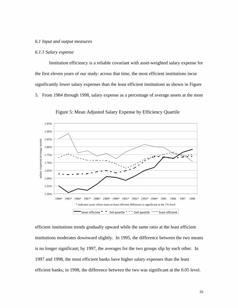
* indicates years where most-to-least efficient difference is significant at the 1% level

most efficient 3rd quartile 2nd quartile least efficient

14

score quartile, suggesting that our convention of quartile-based analysis is also

appropriate.4

An analysis by average asset size also reveals interesting differences between

efficiency groups. In each year of the study, the smallest institutions are most efficient,

and the largest are least efficient, as displayed in Figure 3. Further, the relative positions

of the means of the second and third quartiles remain statistically significant and rank-

distinct5 across the 15 years of the study. This result seems to underscore the potential

for greater inefficiencies in the operation of larger, more complex organizations.

4 When reviewing data based on efficiency scores it is important to bear in mind that the DEA model derives an efficiency score for aparticular institution relative to other institutions in a finite reference group. The score therefore cannot be generalized to periods orinstitutions external to the original reference group, i.e., scores cannot be compared year to year: a score of 0.8 in one year is notnecessarily more efficient than a score of 0.4 the following year.5 Quartile data are rank-distinct in a given period if the four groups of dependent variables remain distinct and congruent with theindependent variable across that time, e.g., the institutions in the lowest efficiency score-based quartile have the highest average salaryexpense, the adjacent efficiency score quartile has the second highest average salary expense, etc.

Figure 3: Score by Size Quartile

0.00

0.05

0.10

0.15

0.20

0.25

0.30

0.35

0.40

1984* 1985* 1986* 1987* 1988* 1989* 1990* 1991* 1992* 1993* 1994* 1995* 1996* 1997* 1998*

* indicates years where largest-to-smallest difference is significant at the 1% level

largest 3rd quartile 2nd quartile smallest

15

Efficiency scores of banks rated as strong and weak by examiners also exhibit

significant differences across the study. As shown in Figure 4, in each year, “strong”

institutions (those with composite CAMELS ratings of “1” or “2”) are significantly more

efficient than “weak” institutions (rated “3”, “4”, or “5”). These results, discussed in

greater detail below, are consistent with the expectation that efficiency and perceived

soundness are covariants.

Figure 4: Score by Overall CAMELS Rating

0.00

0.05

0.10

0.15

0.20

0.25

0.30

0.35

1984* 1985* 1986* 1987* 1988* 1989* 1990* 1991* 1992* 1993* 1994* 1995* 1996* 1997* 1998*

* indicates years where strong-to-weak difference is significant at the 1% level

strong weak

16

6.1 Input and output measures

6.1.1 Salary expense

Institution efficiency is a reliable covariant with asset-weighted salary expense for

the first eleven years of our study: across that time, the most efficient institutions incur

significantly lower salary expenses than the least efficient institutions as shown in Figure

5. From 1984 through 1998, salary expense as a percentage of average assets at the most

efficient institutions trends gradually upward while the same ratio at the least efficient

institutions moderates downward slightly. In 1995, the difference between the two means

is no longer significant; by 1997, the averages for the two groups slip by each other. In

1997 and 1998, the most efficient banks have higher salary expenses than the least

efficient banks; in 1998, the difference between the two was significant at the 0.05 level.

Figure 5: Mean Adjusted Salary Expense by Efficiency Quartile

1.50%

1.55%

1.60%

1.65%

1.70%

1.75%

1.80%

1.85%

1.90%

1.95%

1984* 1985* 1986* 1987* 1988* 1989* 1990* 1991* 1992* 1993* 1994* 1995 1996 1997 1998



17

The first eleven years seem consistent with our hypothesis: the most efficient banks were

the ones that were the best at containing costs, in this case, salary expenses. The last four

years’ results are less clear. It may be that in 1995-1998 the more efficiently managed

institutions started paying higher salaries to attract and retain better qualified employees

in a more competitive labor environment.6 At the same time, the lack of growth in mean

adjusted salary expense among less efficient institutions may be indicative of efforts to

contain or attempt to reduce expenses in order to improve operating efficiencies and

profitability.

6.1.2 Fixed assets

As shown in Figure 6, in each of the 15 years, the most efficient banks have

6 One indication of the tight labor market can be seen in the U.S. unemployment rate, which steadily declined from 7.8 percent of thecivilian labor force in mid-1992 to 4.3 percent by the end of 1998.

Figure 6: Mean Adjusted Fixed Assets by Efficiency Quartile

1.0%

1.2%

1.4%

1.6%

1.8%

2.0%

2.2%

2.4%

2.6%

1984* 1985* 1986* 1987* 1988* 1989* 1990* 1991* 1992* 1993* 1994* 1995* 1996* 1997* 1998*



18

significantly lower fixed asset levels than do the least efficient banks. From 1984 to 1998

the difference between the means of the fixed asset ratios of the most and least efficient

banks narrows from 1.07 percent of assets to 0.41 percent of assets, but the difference

remains statistically significant. In fact, from 1984 through 1992 the differences between

each quartile are significant at the 0.01 level. From 1993 through 1998 these differences

deteriorate initially for the third most efficient quartile, and then for the second most

efficient quartile as well, making this measure much less differentiating of efficiency.

From 1993 to 1998, fixed assets as a percentage of total assets increase an average of 2.7

percent for the three most efficient quartiles, while it decreases 0.3 percent for the least

efficient quartile. These results are consistent with our expectation that the minimization

of fixed (non-earning) assets is among the characteristics that distinguish more efficient

institutions.

6.1.3 Other noninterest expense

Other noninterest expense (comprised of noninterest expenses excluding salary

expenses) also evidences a strong relationship with our efficiency measure. As shown in

Figure 7, the quartile of least efficient banks has significantly higher noninterest expenses

than the most efficient banks for all 15 years. Further, the differences between the means

of all four quartiles remain statistically significant at at least the 0.05 level. The mean

differences are also rank-distinct across the 15 years of the study. Although the

difference between most and least efficient quartiles trends moderately toward zero,

improving conditions do not seem to have a dramatic effect on other noninterest

expenses.

19

6.1.4 Interest expense

As shown in Figure 8, no completely consistent relationship is evident between

Figure 7: Mean Adjusted Other Noninterest Expenseby Efficiency Quartile

1.0%

1.2%

1.4%

1.6%

1.8%

2.0%

2.2%

2.4%

2.6%

1984* 1985* 1986* 1987* 1988* 1989* 1990* 1991* 1992* 1993* 1994* 1995* 1996* 1997* 1998*



Figure 8: Mean Adjusted Interest Expense by Efficiency Quartile

0%

1%

2%

3%

4%

5%

6%

7%

8%

1984* 1985 1986* 1987* 1988* 1989* 1990* 1991 1992* 1993* 1994* 1995* 1996* 1997* 1998*



20

efficiency and interest expense, although there appears to be a slight tendency for less

efficient banks to have higher interest expenses. The difference in interest expense

between the most and least efficient quartiles is statistically significant at the 0.01 level in

13 of the 15 years. In ten of these years, the less efficient institutions incur higher

average interest expenses than their most efficient counterparts; in the other three years

(1986, 1992, and 1993), less efficient banks actually incur significantly lower average

interest expenses than the most efficient banks in the study. Although failing to be

completely consistent, the results overall seem to indicate the highly competitive nature

of banks’ interest rate management. With very few exceptions, year-to-year changes in

interest expense move in the same direction for each quartile for each year of the study.7

Contrary to our expectations, more and less efficient banks become more distinct

on the interest expense measure after the 1991-1992 “bad-to-good conditions” change.

This may be driven in some degree by movement in the purchased funds measure

(discussed in the following section) which follows a similar course.

6.1.5 Purchased funds

In our study, the level of an institution’s purchased funds is inversely related to

efficiency. In each year, purchased funds for the least efficient quartile exceeds that of

the most efficient quartile by a significant difference, as shown in Figure 9. The

differences for each quartile are clearly rank-distinct. Indeed, purchased funds in the

least efficient quartile are always significantly greater than purchased funds in the

adjacent (next-most-efficient) quartile. A gross, overall summary of the 15 years of data

7 There were three exceptions to this pattern: in 1990 interest expense increased for the most efficient quartile while declining in theothers, in 1994 interest expense increased for the least efficient quartile contrary to the other quartiles, and in 1998 interest expensedeclined slightly for one of the quartiles while the other quartiles increased.

21

indicates that the least efficient banks, on average, have year-end purchased funds

equaling 23.3 percent of their total assets; the same ratio for the adjacent quartile and the

most efficient quartile is 12.3 percent and 3.5 percent, respectively. This may reflect

unwillingness or difficulty on the part of less efficient institutions to access less costly

sources of funds (e.g., core deposits).

When examining changes over time, more and less efficient banks become more

distinct on this measure after the 1991-1992 “bad-to-good conditions” change. The

difference between the adjusted level of purchased funds of the most and least efficient

quartiles declines steadily from 1986 to 1992, and rises steadily in each subsequent year.

This trend implies more efficient banks are better able (relative to less efficient banks) to

utilize less expensive sources of funds in improving economic conditions.

Figure 9: Mean Adjusted Purchased Funds by Efficiency Quartile

0%

5%

10%

15%

20%

25%

30%

1984* 1985* 1986* 1987* 1988* 1989* 1990* 1991* 1992* 1993* 1994* 1995* 1996* 1997* 1998*



22

6.1.6 Earning assets

As Figure 10 shows, the differences in earning assets between efficiency quartiles

are dynamic over time. In each year, the least efficient institutions have significantly

lower levels of earning assets than the most efficient institutions. Here again, the

efficiency score-derived quartiles yield average earning asset levels that were rank-

distinct. These relationships persist even as the average earning asset level of all four

quartiles improves over time, from 88.7 percent of total average assets in 1984 to 92.0

percent in 1998. The least efficient quartile experiences the greatest improvement,

increasing from 86.4 percent in 1984 to 91.7 percent in 1998. By comparison, the most

efficient quartile increases its percentage of earning assets from 90.4 to 92.3 across the

same period. While the difference between the most and least efficient quartiles steadily

Figure 10: Mean Adjusted Earning Assets by Efficiency Quartile

86%

87%

88%

89%

90%

91%

92%

93%

1984* 1985* 1986* 1987* 1988* 1989* 1990* 1991* 1992* 1993* 1994* 1995* 1996* 1997* 1998*



23

declines over time, the relative movement of the earning assets levels for all of the

quartiles generally improves.

6.1.7 Interest income

Interest income, an output in our DEA model, exhibits characteristics similar to

the related input factor interest expense. As shown in Figure 11, there appears to be no

consistent relationship between efficiency and interest income. However, of the 15 years

under study, the difference between the most and least efficient quartiles is significant in

eight years. In six of these eight years the most efficient group has higher interest income

than the least efficient group.

Figure 11: Mean Adjusted Interest Income by Efficiency Quartile

6%

7%

8%

9%

10%

11%

12%

1984* 1985* 1986* 1987* 1988 1989* 1990 1991* 1992* 1993* 1994 1995 1996 1997 1998



24

If interest income and interest expense are considered together, an interesting

pattern emerges from 1994 to 1998. Across these five years, the relationship between

efficiency and interest expense, after having fluctuated considerably, seems to settle into

a pattern where the most efficient institutions report consistently and significantly lower

interest expenses than the least efficient institutions. During the same time period,

however, interest income is actually greater in the least efficient quartile than the most

efficient quartile, although the differences failed to reach the 0.01 level of significance8.

These results are congruent with a scenario wherein less efficient institutions make

significantly greater recourse to purchased funds (discussed above) on the expense side,

while having a significantly higher percentage of their asset portfolios composed of loans

(discussed below), which tend to carry greater risk and greater interest return than other

assets.

The longitudinal interaction between the weighted interest income levels of the

most and least efficient quartiles is difficult to characterize. The five-year period

identified as the height of the banking crisis (1988-1992) witnesses two of the three years

of greatest difference in interest income between the most and least efficient quartiles. In

1989, the least efficient quartile has the higher interest income level, and in 1992 the

most efficient quartile has the higher interest income level. After 1994, however, the

differences between the two quartiles on this measure tend toward zero.

8 The differences were statistically significant at the 0.05 level in 1995, 1996, and 1997.

25

6.1.8 Noninterest income

Noninterest income is another highly reliable covariant with measured efficiency.

In each year of our study, the least efficient institutions have significantly higher

noninterest income levels (measured as the ratio of noninterest income to average assets)

than the most efficient institutions as shown in Figure 12. This measure also yields

results that are consistently rank-distinct.9 This finding suggests that less efficient

institutions are more willing to increase earnings by emphasizing this output. This

difference is significant: in our study noninterest income averages 1.40 percent of

average assets for the least efficient banks, and 0.68 percent for the most efficient banks.

9 Data for the most efficient quartile in 1989 reflect the removal of two institutions whose reported results were highly anomalous andskewed the data.

Figure 12: Mean Adjusted Noninterest Incomeby Efficiency Quartile

0.0%

0.5%

1.0%

1.5%

2.0%

2.5%

1984* 1985* 1986* 1987* 1988* 1989* 1990* 1991* 1992* 1993* 1994* 1995* 1996* 1997* 1998*



26

6.2 Bank performance measures

6.2.1 Return on average assets

As shown in Figure 13, return on average assets (ROAA) is positively related to

our efficiency measure. In each year of our study, the differences in ROAA between the

most efficient and least efficient groups are significant at the 0.01 level. Moreover, in

each year, ROAA for each of the efficiency score-based quartiles remains rank-distinct.

ROAA is also a good barometer of the effect that the banking crisis in the 1980s

had on banks of varying efficiencies. The three most efficient quartiles reach their lowest

average ROAA in 1986, when average ROAA for the least efficient banks drops just

below zero. In 1987, as the first three quartiles’ averages begin to rebound, the average

for the least efficient group slides further to –0.17 percent. From this low, ROAA for the

least efficient quartile begins to climb, slowly closing the gap with the other three groups.

Figure 13: Mean ROAA by Score Quartile

-0.40

-0.20

0.00

0.20

0.40

0.60

0.80

1.00

1.20

1.40

1.60

1984* 1985* 1986* 1987* 1988* 1989* 1990* 1991* 1992* 1993* 1994* 1995* 1996* 1997* 1998*



27

From a maximum deficit of 109 basis points below the most efficient quartile in 1987,

average ROAA at the least efficient banks climbs to within 15 basis points in 1994, and

averages a difference of 18 basis points from 1994 through 1998.

Perhaps the least efficient banks have the most room for improvement, which

enables them to impact their situation more effectively and recover more ground as

banking conditions improve. Moreover, as the banking industry consolidated and

became more competitive, the differences in performance between the most and least

efficient banks would be expected to narrow.

6.2.2 Nonperforming loans to gross loans

The percentage of gross loans that are nonperforming reflects a strong difference

between relatively efficient and inefficient banks across varying industry conditions. As

shown in Figure 14, nonperforming loans in 1984 account on average for 2.58 percent of

Figure 14: Mean Nonperforming Loans to Gross Loansby Efficiency Quartile

0.5%

1.0%

1.5%

2.0%

2.5%

3.0%

3.5%

4.0%

1984* 1985* 1986* 1987* 1988* 1989* 1990* 1991* 1992* 1993* 1994 1995 1996 1997 1998



28

gross loans for the most efficient quartile of banks, compared to 2.88 percent for the least

efficient banks. The gap between the two widens with the declining conditions for banks

until 1987, when nonperforming loans are on average 2.35 percent of gross loans for the

most efficient banks, compared to 3.69 percent for their least efficient counterparts.

From 1984 through 1993 the difference between the most and least efficient banks

is statistically significant at the 0.01 level, the most efficient institutions having a much

lower level of nonperforming loans. After 1987, the gap between the two begins to

narrow, with the nonperforming loan ratio decreasing at a faster rate at less efficient

institutions than at more efficient institutions. By 1994, the difference is no longer

statistically significant, a condition which persists through the end of the study period in

1998.

6.2.3 Loan to asset ratio

The ratio of loans to total assets shows a significant difference between the least

and most efficient quartiles, with the least efficient group having a higher concentration

of loans as shown in Figure 15. If a higher loan-to-asset ratio is related to a bank’s

willingness to take on additional risk, these findings are consistent with the view that less

efficient institutions are less risk averse than their more efficient counterparts. This may

also indicate greater attempts by less efficient banks to improve their operating

efficiencies and profitability by increasing revenues through riskier ventures.

Considered over time, these results suggest a banking market that is on the whole

growing more amenable to risk, or perhaps better able to manage and control risk through

other channels (e.g., financial derivatives and other risk management practices). The two

most efficient quartiles reach their lowest loan-to-asset ratio in 1987, after which the

29

percentage of their assets held as loans increases. The two least efficient quartiles both

reach their lowest loan-to-asset ratio in 1993, and increase afterward. It may be that the

upward trend by all four groups, and the fact that the loan-to-asset ratios of the second

and third quartiles exceed the least efficient quartile’s ratio in 1997 and 1998, indicate

improved risk management practices and a highly competitive environment.

6.3 Examiner ratings

In the early 1970s regulators of federal financial institutions, realizing the

advantages of a standardized framework for the examination process, developed a rating

system whereby the most critical components of a financial institution’s overall safety

and soundness could be identified, measured, and quantified. In 1979, the Uniform

Financial Institutions Rating System was adopted. Commonly referred to by the acronym

of its component parts, the CAMEL rating, the outcome of an on-site examination of a

Figure 15: Mean Loans/Assets by Efficiency Quartile

45%

47%

49%

51%

53%

55%

57%

59%

61%

63%

1984* 1985* 1986* 1987* 1988* 1989* 1990* 1991* 1992* 1993* 1994* 1995* 1996* 1997* 1998*



30

financial institution, has become a concise and indispensable tool for examiners and

regulators.

The evaluation factors that comprise an institution’s CAMEL rating are:

Capital adequacyAsset qualityManagement qualityEarnings abilityLiquidityNote: In 1997, a sixth component was added – Sensitivity to market risk

Each of the factors is scored from ‘one’ to ‘five’, with ‘one’ being the strongest

rating. Additionally, a single composite CAMELS rating is determined from these

components, and represents the findings of the examination for the institution as a whole.

The Commercial Bank Examination Manual produced by the Board of Governors of the

Federal Reserve System describes the five composite rating levels as follows:

CAMELS = 1 An institution that is basically sound in every respect.

CAMELS = 2 An institution that is fundamentally sound but has moderateweaknesses.

CAMELS = 3 An institution with financial, operational, or complianceweaknesses that give cause for supervisory concern.

CAMELS = 4 An institution with serious financial weaknesses that couldimpair future viability.

CAMELS = 5 An institution with critical financial weaknesses that renderthe probability of failure extremely high in the near term.

Research involving efficiency and CAMELS ratings is somewhat limited, due in

large part to the restricted nature of the ratings themselves.10 DeYoung (1998), using the

management component of the rating, found that, when comparing well and poorly

10 The CAMELS rating of an institution is held in strictest confidence by regulators. The composite rating is divulged only to themanagement of the examined entity; the six component ratings are kept internal to the regulatory agencies.

31

managed banks, well-managed banks had lower estimated unit costs and higher raw

(accounting-based) unit costs, suggesting that cost-efficient management does involve

expenditures that poorly managed banks tend to fail to make.

We evaluate our DEA results against the CAMELS ratings of banks from 1984

through 1998, anticipating that more efficient institutions would tend to have higher

CAMELS ratings than less efficient institutions. CAMELS ratings, assigned by

examiners at the end of an on-site examination, are “snapshot” evaluations of a given

bank at a given point in time, and are thus perishable quantities (see Cole and Gunther,

1995). Given the dynamic nature of the financial industry, the underlying factors on

which the ratings are based begin to change in some ways immediately after the rating is

given. An example of this might be a poorly rated institution that begins immediately to

implement directives for improvement imposed by its examiners. We therefore wanted

to carefully match our year-end data with CAMELS ratings, ensuring that each was

pertinent and referred to “the same bank.”

To do this, we limit the CAMELS portion of our analysis to banks that received a

rating within a twelve-month window beginning six months before the year-end data

under consideration. To compensate for the fact that in many years there are too few

institutions with lower ratings to construct a statistically adequate sample, we divide the

ratings into two groups. Institutions with composite ratings of “1” or “2” are considered

strong banks and institutions with composite ratings of “3”, “4”, or “5” are considered

weak banks. As shown in Figure 4 (earlier in the text), banks with strong CAMELS

ratings have significantly higher efficiency scores than banks with weak ratings. This

relationship was constant across all 15 years in the study.

32

7. Conclusion

In this study, we employ a constrained-multiplier, input-oriented DEA model to

evaluate the relative productive efficiency of U.S. commercial banks across a 15-year

period. The DEA model offers numerous benefits, including the ability to target areas of

relative efficiency between banks. Perhaps most importantly, it allows analysis of

multiple aspects of a financial institution’s performance, unlike more common

benchmarking methodologies that focus on only one of many interrelated measures at a

time. DEA creates an analysis that is broader without sacrificing depth of insight, an

analysis that is more pertinent and hence applicable to the real-world operations of

complex financial institutions.

We divide commercial banks into quartiles based on their DEA-derived efficiency

score, and find that in each year of our 15-year review each quartile has significantly

higher efficiency scores than the quartile beneath it. A similar, rank-distinct relationship

is discovered between efficiency quartiles on the weighted measures of noninterest

income, other noninterest expense, and purchased funds (all three inversely related to

efficiency), as well as earning assets and return on average assets (both positively related

to efficiency). The relationship between efficiency and interest income and expense is

not as pervasive, perhaps as a result of market competition, but there is still a noticeable

tendency for efficiency to be positively correlated with interest income and negatively

related to interest expense. There is also a strong negative relationship between the most

efficient and least efficient quartiles of banks on the percentage of assets that were fixed

assets and the percentage of total assets that were loans.

33

The level of nonperforming loans to total loans is significant and negatively

related to the efficiency scores of the most and least efficient quartiles from 1984 through

1993. The relationship of efficiency to salary expense is similar from 1984 through 1994.

It is likely that nonperforming loans and salary expense lose their predictive power vis-à-

vis efficiency as a result of the same external forces: the improving economy, improving

conditions of financial institutions after the difficulties of the 1980s, and financial

industry consolidation.

We examine the change in our independent variables over time, particularly

noting the change in the difference between the most and least efficient quartiles. We

find that only return on average assets, the ratio of nonperforming loans-to-gross loans,

and the relative level of purchased funds seem to be impacted by improved economic

conditions. The “most-efficient-to-least-efficient” differences of the other variables in

the study seem to trend across the 15-year period independent of economic conditions.

Consistent with previous research, we find a significant relationship between

CAMELS ratings and efficiency scores: institutions rated by examiners as the strongest

have higher efficiency scores than those institutions rated as the weakest in each year of

our study. This finding suggests that DEA might be a useful off-site bank surveillance

tool to monitor banks between on-site examinations.

DEA represents a potential for significant advance in the comparative analysis of

financial institutions. Limited until fairly recently by the lack of affordable, large scale

computational resources, frontier estimation techniques such as DEA offer analysts the

ability to appreciate an organization in greater depth by enabling the concurrent study of

the multiple variables that impact a firm’s efficiency, and hence its competitiveness,

34

potential, and even viability. As already noted, DEA models can be used to develop off-

site monitoring tools for use by regulators and examiners. Banks can employ such

models internally to benchmark their own processes, finding potential areas for

improvement as well as gauging the potential and efficacy of their efforts as they operate

in an industry which is increasingly characterized by accelerating change and

competition. Finally, industry analysts and policymakers can use DEA as a powerful tool

for understanding more about the behavior of institutions and markets in this rapidly

changing and increasingly complex industry.

35

References

Barr, R.S., Seiford, L.M., Siems, T.F., 1993. An Envelopment-Analysis Approach toMeasuring the Managerial Efficiency of Banks. Annals of Operations Research 45, 1-19.

Bauer, P.W., Berger, A.N., Ferrier, G.D., Humphrey, D.B., 1998. Consistency Conditionsfor Regulatory Analysis of Financial Institutions: A Comparison of Frontier EfficiencyMethods. Journal of Economics and Business 50(2), 85-114.

Bean, M.L., Duncan-Hodge, M., Ostermiller, W.R., Spaid, M., Stockton, R.S., 1998.Managing the Crisis: The FDIC and RTC Experience (Federal Deposit InsuranceCorporation, Washington).

Berger, A.N., Demsetz, R.S., Strahan, P.E., 1999. The Consolidation of the FinancialServices Industry: Causes, Consequences, and Implications for the Future. Journal ofBanking and Finance 23, 135-194.

Berger, A.N., Humphrey, D.B., 1997. Efficiency of Financial Institutions: InternationalSurvey and Directions for Future Research. European Journal of Operational Research98(2), 175-212.

Berger, A.N., Mester, L.J., 1997. Inside the Black Box: What Explains Differences in theEfficiencies of Financial Institutions? Journal of Banking and Finance 21, 895-947.

Bowlin, W.F., 1998. Measuring Performance: An Introduction to Data EnvelopmentAnalysis (DEA). Journal of Cost Analysis, 3-27.

Cebenoyan, A.S., Cooperman, E.S., Register, C.A., 1993. Firm Inefficiency and theRegulatory Closure of S&Ls: An Empirical Investigation. Review of Economics andStatistics 75, 540-545.

Charnes, A., Cooper, W.W., 1962. Programming with Linear Fractional Functionals.Naval Research Logistics Quarterly 9(3/4), 181-185.

Charnes, A., Cooper, W.W., Golany, B., Seiford, L., Stutz, J., 1985. Foundations of DataEnvelopment Analysis for Pareto-Koopmans Efficient Empirical Production Functions.Journal of Econometrics 20, 91-107.

Charnes, A., Cooper, W.W., Lewin, A.Y., Seiford, L.M., 1994. Data EnvelopmentAnalysis: Theory, Methodology and Applications (Kluwer Academic Publishers,Norwell, MA).

Charnes, A., Cooper, W.W., Rhodes, E., 1978. Measuring the Efficiency of DecisionMaking Units. European Journal of Operational Research 2(6), 429-444.

36

Cole, R.A., Gunther, J.W., 1995. A CAMEL Rating’s Shelf Life. Financial IndustryStudies, 13-20.

DeYoung, R., 1998. Management Quality and X-Inefficiency in National Banks. Journalof Financial Services Research 13(1), 5-22.

Farrell, M.J., 1957. The Measurement of Productive Efficiency. Journal of the RoyalStatistical Society, Series A, General, Part 3, 253-281.

Humphrey, D.B., Pulley, L.B., 1997. Banks’ Responses to Deregulation: Profits,Technology, and Efficiency. Journal of Money, Credit, and Banking, 73-93.

Resti, A., 1998. Regulation Can Foster Mergers, Can Mergers Foster Efficiency? TheItalian Case. Journal of Economics and Business 50(2), 157-169.

Siems, T.F., Barr, R.S., 1998. Benchmarking the Productive Efficiency of U.S. Banks.Financial Industry Studies, Federal Reserve Bank of Dallas, 11-24.

37

Table 1

Variable Definitions

Call Report Item CodeINPUTS

Salary Expense RIAD4135Premises and Fixed Assets RCFD2145Other Noninterest Expense RIAD4093 – RIAD4135Interest Expense RIAD4073Purchased Funds* RCFD0278 + RCFD0279 + RCON2840 +

RCFD2850 + RCON6645 + RCON6646

OUTPUTSEarning Assets** RCFD2122 – (RCFD1407 + RCFD1403) +

RCFD0390 + RCFD0071 + RCFD0276 +RCFD0277 + RCFD2146

Interest Income RIAD4107Noninterest Income RIAD4079

* Purchased Funds are federal funds purchased and securities sold under agreement torepurchase, demand notes issued to the U.S. Treasury, other borrowed money, timecertificates of deposit of $100,000 or more, and open-account time deposits of $100,000or more.

** Earning Assets are total loans less loans past due 90 days or more and loans innonaccrual status, plus total securities, interest-bearing balances, federal funds sold andsecurities purchased under agreements to resell, and assets held in trading accounts.

38

Table 2

Constraints for the Multipliers (Weights) in the DEA Model

Lower Bound Upper BoundInputs

Salary Expense 15.8% 35.9%Premises/Fixed Assets 3.1% 15.7%Other Noninterest Expense 15.8% 35.9%Interest Expense 17.2% 42.8%Purchased Funds 12.1% 34.0%

OutputsEarning Assets 40.9% 69.5%Interest Income 25.7% 46.9%Noninterest Income 10.2% 20.2%

39

Table 3

Hypotheses: Relative Characteristics of More Efficient Banks

Characteristic More Efficient Institutions Less Efficient InstitutionsSalary expense Lower Higher

Other noninterest expense Lower HigherNoninterest income Higher Lower

Interest expense Lower HigherInterest income Higher Lower

Fixed assets Lower HigherEarning assets Higher Lower

Purchased funds Lower HigherROAA Higher Lower

Nonperforming loans Lower HigherLoans to assets Lower Higher

CAMELS ratings Stronger Weaker

Date post:	18-Jan-2022
Category:	Documents
Upload:	others
View:	3 times
Download:	0 times

Evaluating the Productive Efficiency and Performance of U ...

Documents