Anatomy-based Regularization Methods for Dynamic PET ...

Eighth Hungarian Conference on Computer Graphics and Geometry, Budapest, 2016

Anatomy-based Regularization Methods for Dynamic PETReconstruction

Ágota Kacsó and László Szirmay-Kalos

Budapest University of Technology and Economics (e-mail: [email protected])

AbstractThis paper examines and compares regularization methods for direct parametric dynamic PET reconstruction,when the space-time activity function needs to be recovered from measurements. In binned mode reconstruction,the measurement time is decomposed to frames and events are binned. In order to mimic high-speed phenom-ena, frames must be short, thus the number of events in a frame is very low, making frame-wise reconstructionimpossible. To attack this problem, regularization is needed that enforces smoothness both in the temporal andspatial domains. For temporal regularization, different kinetic models are used. For spatial regularization, wecan subtract a penalty term from the likelihood of the measured data that penalizes unacceptable solutions, orthe reconstruction can be filtered in every iteration to project the actual estimate into the subspace of acceptablesolutions. The objective of this paper is to analyze these options and compare their effectiveness.

1. Introduction

In dynamic Positron Emission Tomography (PET), we mea-sure how the density of a radiotracer changes in time at dif-ferent voxels of the examined object, thus dynamic tomog-raphy reconstructs a space-time density xV (t). The spatialvariation of the density is defined on a grid 20, 2, 3, 4, 26, 15, forexample, in voxels. Using the space-time density, the ex-pected number of radioactive decays in voxel V in differ-ential time dt is xV (t)dt. The positron emitted at a decay an-nihilates with an electron generating two oppositely directedgamma-photons, which might be detected by the tomograph.A PET/CT system collects the events of simultaneous pho-ton incidents in detector pairs, called Line Of Response orLOR. The measurement time is decomposed into finite timeintervals, called frames ∆t1, . . . ,∆tNT with interval centerst1, . . . , tT , and events are binned in frames. We denote thenumber of events in LOR L and frame T by yL,T .

If fast dynamic changes are to be recovered, frames mustbe short and consequently the number of events in a frameis rather low. This means that reconstruction done indepen-dently in frames is either impossible or leads to very noisydata. To attack this problem, regularization is needed thatenforces the smoothness both in the temporal and the spatialdomains.

2. Dynamic PET reconstruction

The state of the art and previous work on direct estimationof kinetic parametric images for dynamic PET are surveyedin review article 28.

The event rate λL(t) in LOR L at time t is the sum of thecontributions of all voxels in the volume at this time:

λL(t) =NV

∑V=1

ALV xV (t)

where system matrix AL,V expresses the probability that adecay in voxel V generates an event in LOR L.

During iterative Expectation Maximization (ML-EM) re-construction 16, unknown coefficients are found to maximizethe probability of the actually measured data. Assuming thatthe measured number of hits in LOR L in time interval ∆tTfollows a Poisson distribution and is statistically indepen-dent of other LORs and frames, the log-likelihood of thecurrent measurement is

logL= ∑L

∑T

(yL,T logλL(tT )−λL(tT )∆tT

). (1)

The high variance of the involved random variables makesthe optimization process fit the solution to noise, resultingin unacceptably high variation reconstructions. The tempo-

Kacsó, Szirmay-Kalos / Anatomy-based Regularization Methods for Dynamic PET Reconstruction

ral and spatial variation of the solution must be kept undercontrol, which is the responsibility of regularization.

2.1. Temporal regularization

For temporal regularization, we assume that the time activityfunction of voxel V can be expressed by a common kineticmodel

xV (t) = F(θV , t),

where spatially dependent properties are encoded in alow dimensional vector of parameters θ. Such models canbe based on the mathematical description of the biologi-cal/chemimal processes or on compartment analysis 5, 30, 29.

2.2. Spatial regularization with a penalty term

One possibility to impose spatial regularization is to includea penalty term R(θ) into the optimization target function.Thus, we find the extremum of the following functional:

E(θ) = logL(θ)−R(θ). (2)

The penalty term should be high for unacceptable solu-tions and small for acceptable ones. Standard regularizationmethods like Tikhonov regularization and Truncated Singu-lar Value Decomposition (TSVD) assume the data set tobe smooth and continuous, and thus enforce these prop-erties during reconstruction. However, the typical data inPET reconstruction are different, there are sharp features thatshould not be smoothed with the regularization method. Weneed a penalty term that minimizes the unjustified oscillationwithout blurring sharp features. An appropriate penalty termis the total variation (TV) of the solution 14, 11, 10, 12. Totalvariation regularization may create stair-like artifacts, whichcan be reduced by Bregman iteration 23.

The inclusion of the anatomic information into spatialregularization is straightforward, smoothness should be im-posed only inside anatomically homogeneous regions butnot on their boundaries 1.

2.3. Method of sieves

In this approach, the optimization target is not modified, butthe iterated approximation is filtered in each iteration step.Several authors proposed the inclusion of a voxel space fil-tering step in the reconstruction loop 17, 9 and it turned outthat it is equivalent to the method of sieves that seeks to con-strain the EM solution to a subspace of all possible solutions18, 19, 27. The objective of filtering is to find an acceptable so-lution that is close to the solution proposed by the iteration.Filtering can also exploit anatomic information gathered bya CT or an MR 24.

2.4. The proposed method

The reconstruction means the solution of the optimizationproblem of Equation 2. The optimization target has an ex-tremum where all partial derivatives are zero:

∂E(θ)∂θV,P

= 0.

Computing the partial derivatives, we obtain(∑L

AL,V

)∑T

∂F∂θV,P

∣∣∣∣tT

(xV,T (θ)

F(θV , tT )−∆tT

)− ∂R

∂θV,P= 0,

(3)where xV,T is the result of a static forward projection andback projection taking the data from frame T :

λL,T = ∑V ′

AL,V ′F(θV ′ , tT )

xV,T = F(θV , tT ) ·∑L AL,V

yL,TλL,T

∑L AL,V.

In this equation kinetic model F depends on unknown pa-rameter vector of the given voxel θV , while xV,T and R de-pend on the parameter vectors of all voxels. Additionally,xV,T is the only factor that is affected by the elements ofthe system matrix. Thus, if xV,T and R were known, then thecomputation could be decoupled for different voxels and canbe made independent of the huge system matrix.

To achieve this, a subiteration is included into the mainiteration solution of this equation. In the subiteration expen-sive terms like xV,T and R are not re-evaluated, they are up-dated just in the main iteration steps, which update xV,T andR. The task of the subiteration is the solution of the followingfunction for θ(n+1)

V :(∑L

AL,V

)∑T

∂F(θ(n+1)V )

∂θV,P

∣∣∣∣∣tT

(xV,T (θ(n))

F(θ(n+1)V , tT )

−∆tT

)−

∂R(θ(n)V )

∂θV,P= 0. (4)

Assuming that xV,T is constant, Equation 4 describes justa single voxel, and can thus be solved independently for allvoxels. We use the Iterative Coordinate Descent algorithmfor the solution, which leads to set of parameters for thisparticular voxels, which define a time activity curve F(θV , t)that fits to xV,T .

For the regularization, we consider the options of tempo-ral regularization via kinetic models, spatial regularizationwith the penalty of the total variation of the activity, thepenalty of the total variation of the parameters, filtering theactivity, and filtering the parameters.


2.5. Temporal regularization with various kineticmodels

Time activity F(θ, t) depends on the concentration C(θ, t)of the radiotracer and on the known decay constant λ of theradiotracer:

F(θ, t) =C(θ, t)exp(−λt).

The concentration is searched in a finite function seriesform defined by parameter vector θ. The basis functions ofthis approximation can be general, like B-splines of Mixtureof Gaussians, or can be derived from the biological modelsof the diffusion.

2.5.1. Mixture of Gaussians

In this case, the basis functions are temporal Gaussians de-fined by fixed time value tP and temporal deviation σP:

C(θ, t) = ∑P

aP ·exp(− (t−tP)2

2σ2P

)√

2πσP, θ = (a1, . . . ,aNP)

Deviation σP should be selected to guarantee that the dropto the next time values is not too large.

2.5.2. Spectral method

In spectral method, we also assume the knowledge of theblood input function Cp(t) that describes the radiotracer con-centration in the blood from where diffusion can start. Thebasis functions are convolutions of exponentials of prede-fined exponents αP and the known blood input function:

C(θ, t) = ∑P

aP ·αP exp(−αPt)∗Cp(t), θ = (a1, . . . ,aNP).

The Binding Potential (BP) can be directly computed fromthe coefficients of the spectral method:

BP =−1+NP

∑P=1

aP

2.5.3. Patlak method

The Patlak method is appropriate for the case of irreversiblecompartment at steady state, when the two basis functionsare the blood input function and its integral:

C(θ, t) = a1

t∫0

Cp(τ)dτ+a2Cp(t), θ = (a1,a2).

We assume that the steady state is reached when Cp starts todecrease. Parameter a1 is proportional to the metabolic rate.

2.5.4. Relative equilibrium plot

The Relative Equilibrium Plot is a modified version of theLogan Plot and can be used to describe reversible tracers atsteady state. The basis functions are the blood input functionand its negative derivative:

C(θ, t) = a1Cp(t)−a2dCp(t)

dt, θ = (a1,a2).

Due to the steady state assumption, this model is valid whent is in the range where Cp(t) is already decreasing thus itsderivative is negative. The binding potential can be com-puted from a1 as BP = a1 −1.

2.5.5. Two-tissue-compartment model

The two-tissue-compartment model is based on the solutionof differential equations describing material exchange be-tween compartments.

C(θ, t)= a1 ·α1 exp(−α1t)∗Cp(t)+a2 ·α2 exp(−α2t)∗Cp(t),

θ = (a1,a2,α1,α2).

2.6. Spatial regularization with penalizing the totalvariation

Total variation can be calculated for the reconstructed activ-ity function xV (t):

TV (x) =∫

|∇x|dv ≈

∑V

√(xV r − xV )2 +(xVu − xV )2 +(xV f − xV )2

assuming that voxels are cubic and at unit distance and de-noting the right, upper and front neighbors of voxel V by V r,Vu, and V f , respectively.

Alternatively, we can obtain the weighted sum of varia-tions of individual parameters:

TV (θ) = ∑P

ρP

∫|∇θP|dv

where ρP is the weight of parameter P.

2.7. Spatial filtering

We apply a Gaussian filtering scheme separately for the ac-tivity 9, 8, 13 in the first alternative and for each parameter inthe second.

For each voxel, the activities in the neighboring voxelsof the same anatomic regions are taken and summed havingweighted by a distance dependent Gaussian G(V ′,V ). Thesum of weighted parameter values is finally divided by thesum of weights, and the result replaces the original unfilteredparameter value:

x̂V =∑V ′ xV ′G(V ′,V )

∑V ′ G(V ′,V )


where weight G(V ′,V ) is the Gaussian of the distance be-tween the centers of voxels V and V ′ if these voxels belongto the same anatomic structure and zero otherwise.

In case of parametric filtering, the same procedure is exe-cuted for each voxel and parameter.

θ̂V,P =∑V ′ θV ′,PG(V ′,V )

∑V ′ G(V ′,V ).

3. Results

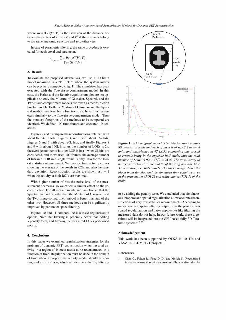
To evaluate the proposed alternatives, we use a 2D brainmodel measured in a 2D PET 22 where the system matrixcan be precisely computed (Fig. 1). The simulation has beenexecuted with the Two-tissue-compartment model. In thiscase, the Patlak and the Relative equilibrium plot are not ap-plicable so only the Mixture of Gaussian, Spectral, and theTwo-tissue-compartment models are taken as reconstructionkinetic models. Both the Mixture of Gaussian and the Spec-tral method use four basis functions, i.e. have four param-eters similarly to the Two-tissue-compartment model. Thusthe memory footprints of the methods to be compared areidentical. We defined 100 time frames and executed 10 iter-ations.

Figures 2 and 3 compare the reconstructions obtained withabout 8k hits in total, Figures 4 and 5 with about 16k hits,Figures 6 and 7 with about 80k hits, and finally Figures 8and 9 with about 160k hits. As the number of LORs is 2k,the average number of hits per LOR is just 4 when 8k hits areconsidered, and as we used 100 frames, the average numberof hits in a LOR in a single frame is only 0.04 for the low-est statistics measurement. We provide time activity curvesshowing the average of the voxels in ROIs and also the stan-dard deviation. Reconstruction results are shown at t = 1when the activity at both ROIs are maximal.

With higher number of hits the noise level of the mea-surement decreases, so we expect a similar effect on the re-construction. For all measurements, we can observe that theSpectral method is better than the Mixture of Gaussian, andthe Two-tissue-compartment model is better than any of theother two. However, all three methods can be significantlyimproved by parameter space filtering.

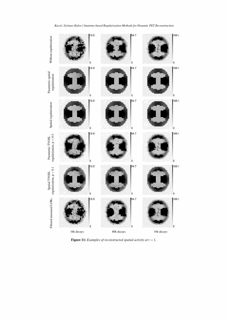
Figures 10 and 11 compare the discussed regularizationoptions. Note that filtering is generally better than addinga penalty term, and filtering the measured LORs performedpoorly.

4. Conclusions

In this paper we examined regularization strategies for theproblem of dynamic PET reconstruction when the total ac-tivity in a region of interest needs to be reconstructed as afunction of time. Regularization must be done in the domainof time where a proper time activity model should be cho-sen, and also in space, which is possible either by filtering

0

2

4

6

8

10

12

14

0 1 2 3 4 5 6 7 8 9 10

activ

ity [B

q/m

l]

time [s]

reference ROI=1reference ROI=2

Cp(t)

Figure 1: 2D tomograph model: The detector ring contains90 detector crystals and each of them is of size 2.2 in voxelunits and participates in 47 LORs connecting this crystalto crystals being in the opposite half circle, thus the totalnumber of LORs is 90× 47/2 = 2115. The voxel array tobe reconstructed is in the middle of the ring and has 32×32 resolution, i.e. 1024 voxels. The lower image shows theblood input function and the simulated time activity curvesin the gray matter (ROI 2) and white matter (ROI 1) of thebrain.

or by adding the penalty term. We concluded that simultane-ous temporal and spatial regularization allow accurate recon-structions of very low statistics measurements. According toour experience, spatial filtering outperforms the penalty termspatial regularization and naive approaches like filtering themeasured data do not help. In our future work, these algo-rithms will be integrated into the GPU based fully-3D Tera-tomo system 6, 7, 25.

Acknowledgement

This work has been supported by OTKA K–104476 andVKSZ-14 PET/MRI 7T projects.

References

1. Chan C., Fulton R., Feng D. D., and Meikle S. Regularizedimage reconstruction with an anatomically adaptive prior for


Para

met

ric

reco

nstr

uctio

nw

ithpa

ram

etri

cre

gula

riza

tion

0

2

4

6

8

10

12

14

0 1 2 3 4 5 6 7 8 9 10

activ

ity [B

q/m

l]

time [s]

reconstruction ROI=1reference ROI=1


Cp(t)

0

2

4

6

8

10

12

14

0 1 2 3 4 5 6 7 8 9 10

activ

ity [B

q/m

l]

time [s]



Cp(t)

0

2

4

6

8

10

12

14

0 1 2 3 4 5 6 7 8 9 10

activ

ity [B

q/m

l]

time [s]



Cp(t)

Para

met

ric

reco

nstr

uctio

nw

ithou

tpa

ram

etri

cre

gula

riza

tion

0

2

4

6

8

10

12

14

0 1 2 3 4 5 6 7 8 9 10

activ

ity [B

q/m

l]

time [s]



Cp(t)

0

2

4

6

8

10

12

14

0 1 2 3 4 5 6 7 8 9 10

activ

ity [B

q/m

l]

time [s]



Cp(t)

0

2

4

6

8

10

12

14

0 1 2 3 4 5 6 7 8 9 10

activ

ity [B

q/m

l]

time [s]



Cp(t)

Mixture of Gaussians Spectral Two-tissue-compartment

Figure 2: Time activity functions of voxels in different ROIs, the average and the standard deviation are depicted, the totalnumber of hits is 8k.

Para

met

ric

reco

nstr

uctio

nw

ithpa

ram

etri

cre

gula

riza

tion

Para

met

ric

reco

nstr

uctio

nw

ithou

tpa

ram

etri

cre

gula

riza

tion

Mixture of Gaussians Spectral Two-tissue-compartment Reference

Figure 3: Examples of reconstructed spatial activity at t = 1, when the total number of hits is 8k.

Kacsó, Szirmay-Kalos / Anatomy-based Regularization Methods for Dynamic PET ReconstructionPa

ram

etri

cre

cons

truc

tion

with

para

met

ric

regu

lari

zatio

n

0

5

10

15

20

25

0 1 2 3 4 5 6 7 8 9 10

activ

ity [B

q/m

l]

time [s]



Cp(t)

0

5

10

15

20

25

0 1 2 3 4 5 6 7 8 9 10

activ

ity [B

q/m

l]

time [s]



Cp(t)

0

5

10

15

20

25

0 1 2 3 4 5 6 7 8 9 10

activ

ity [B

q/m

l]

time [s]



Cp(t)

Para

met

ric

reco

nstr

uctio

nw

ithou

tpa

ram

etri

cre

gula

riza

tion

0

5

10

15

20

25

0 1 2 3 4 5 6 7 8 9 10

activ

ity [B

q/m

l]

time [s]



Cp(t)

0

5

10

15

20

25

30

0 1 2 3 4 5 6 7 8 9 10

activ

ity [B

q/m

l]

time [s]



Cp(t)

0

5

10

15

20

25

0 1 2 3 4 5 6 7 8 9 10

activ

ity [B

q/m

l]

time [s]



Cp(t)



Para

met

ric

reco

nstr

uctio

nw

ithpa

ram

etri

cre

gula

riza

tion

Para

met

ric

reco

nstr

uctio

nw

ithou

tpa

ram

etri

cre

gula

riza

tion




ram

etri

cre

cons

truc

tion

with

para

met

ric

regu

lari

zatio

n

0

20

40

60

80

100

120

140

0 1 2 3 4 5 6 7 8 9 10

activ

ity [B

q/m

l]

time [s]



Cp(t)

0

20

40

60

80

100

120

140

0 1 2 3 4 5 6 7 8 9 10

activ

ity [B

q/m

l]

time [s]



Cp(t)

0

20

40

60

80

100

120

140

0 1 2 3 4 5 6 7 8 9 10

activ

ity [B

q/m

l]

time [s]



Cp(t)

Para

met

ric

reco

nstr

uctio

nw

ithou

tpa

ram

etri

cre

gula

riza

tion

0

20

40

60

80

100

120

140

0 1 2 3 4 5 6 7 8 9 10

activ

ity [B

q/m

l]

time [s]



Cp(t)

0

20

40

60

80

100

120

140

0 1 2 3 4 5 6 7 8 9 10

activ

ity [B

q/m

l]

time [s]



Cp(t)

0

20

40

60

80

100

120

140

0 1 2 3 4 5 6 7 8 9 10

activ

ity [B

q/m

l]

time [s]



Cp(t)



Para

met

ric

reco

nstr

uctio

nw

ithpa

ram

etri

cre

gula

riza

tion

Para

met

ric

reco

nstr

uctio

nw

ithou

tpa

ram

etri

cre

gula

riza

tion




ram

etri

cre

cons

truc

tion

with

para

met

ric

regu

lari

zatio

n

0

50

100

150

200

250

0 1 2 3 4 5 6 7 8 9 10

activ

ity [B

q/m

l]

time [s]



Cp(t)

0

50

100

150

200

250

0 1 2 3 4 5 6 7 8 9 10

activ

ity [B

q/m

l]

time [s]



Cp(t)

0

50

100

150

200

250

0 1 2 3 4 5 6 7 8 9 10

activ

ity [B

q/m

l]

time [s]



Cp(t)

Para

met

ric

reco

nstr

uctio

nw

ithou

tpa

ram

etri

cre

gula

riza

tion

0

50

100

150

200

250

0 1 2 3 4 5 6 7 8 9 10

activ

ity [B

q/m

l]

time [s]



Cp(t)

0

50

100

150

200

250

0 1 2 3 4 5 6 7 8 9 10

activ

ity [B

q/m

l]

time [s]



Cp(t)

0

50

100

150

200

250

0 1 2 3 4 5 6 7 8 9 10

activ

ity [B

q/m

l]

time [s]



Cp(t)



Para

met

ric

reco

nstr

uctio

nw

ithpa

ram

etri

cre

gula

riza

tion

Para

met

ric

reco

nstr

uctio

nw

ithou

tpa

ram

etri

cre

gula

riza

tion




With

outr

egul

ariz

atio

n

0

5

10

15

20

25

0 1 2 3 4 5 6 7 8 9 10

activ

ity [B

q/m

l]

time [s]



Cp(t)

0

20

40

60

80

100

120

140

0 1 2 3 4 5 6 7 8 9 10

activ

ity [B

q/m

l]

time [s]



Cp(t)

0

50

100

150

200

250

0 1 2 3 4 5 6 7 8 9 10

activ

ity [B

q/m

l]

time [s]



Cp(t)

Para

met

ric

spat

ial

regu

lari

zatio

n

0

5

10

15

20

25

0 1 2 3 4 5 6 7 8 9 10

activ

ity [B

q/m

l]

time [s]



Cp(t)

0

20

40

60

80

100

120

140

0 1 2 3 4 5 6 7 8 9 10

activ

ity [B

q/m

l]

time [s]



Cp(t)

0

50

100

150

200

250

0 1 2 3 4 5 6 7 8 9 10

activ

ity [B

q/m

l]

time [s]



Cp(t)

Spat

ialr

egul

ariz

atio

n

0

5

10

15

20

25

0 1 2 3 4 5 6 7 8 9 10

activ

ity [B

q/m

l]

time [s]



Cp(t)

0

20

40

60

80

100

120

140

0 1 2 3 4 5 6 7 8 9 10

activ

ity [B

q/m

l]

time [s]



Cp(t)

0

50

100

150

200

250

0 1 2 3 4 5 6 7 8 9 10

activ

ity [B

q/m

l]

time [s]



Cp(t)

TV

OSL

regu

lari

zatio

n,ρ=

0.1

0

5

10

15

20

25

0 1 2 3 4 5 6 7 8 9 10

activ

ity [B

q/m

l]

time [s]



Cp(t)

0

20

40

60

80

100

120

140

0 1 2 3 4 5 6 7 8 9 10

activ

ity [B

q/m

l]

time [s]



Cp(t)

0

50

100

150

200

250

0 1 2 3 4 5 6 7 8 9 10

activ

ity [B

q/m

l]

time [s]



Cp(t)

Para

met

ric

TV

OSL

regu

lari

zatio

n,ρ=

0.5

0

5

10

15

20

25

0 1 2 3 4 5 6 7 8 9 10

activ

ity [B

q/m

l]

time [s]



Cp(t)

0

20

40

60

80

100

120

140

0 1 2 3 4 5 6 7 8 9 10

activ

ity [B

q/m

l]

time [s]



Cp(t)

0

50

100

150

200

250

0 1 2 3 4 5 6 7 8 9 10

activ

ity [B

q/m

l]

time [s]



Cp(t)

Filte

red

mea

sure

dL

OR

s

0

5

10

15

20

25

0 1 2 3 4 5 6 7 8 9 10

activ

ity [B

q/m

l]

time [s]



Cp(t)

0

20

40

60

80

100

120

140

0 1 2 3 4 5 6 7 8 9 10

activ

ity [B

q/m

l]

time [s]



Cp(t)

0

50

100

150

200

250

0 1 2 3 4 5 6 7 8 9 10

activ

ity [B

q/m

l]

time [s]



Cp(t)

16k decays 80k decays 160k decays

Figure 10: Comparison of different regularization options for the two-tissue compartment model


With

outr

egul

ariz

atio

nPa

ram

etri

csp

atia

lre

gula

riza

tion

Spat

ialr

egul

ariz

atio

nPa

ram

etri

cT

VO

SLre

gula

riza

tion,

ρ=

0.5

Spat

ialT

VO

SLre

gula

riza

tion,

ρ=

0.1

Filte

red

mea

sure

dL

OR

s

16k decays 80k decays 16k decays

Figure 11: Examples of reconstructed spatial activity at t = 1.


positron emission tomography. Phys. Med. Biol., 54:7379–400, 2009.

2. B. Csébfalvi. An evaluation of prefiltered reconstructionschemes for volume rendering. IEEE Transactions on Visu-alization and Computer Graphics, 14(2):289–301, 2008.

3. B. Csébfalvi. An evaluation of prefiltered B-spline reconstruc-tion for quasi-interpolation on the body-centered cubic lattice.IEEE Transactions on Visualization and Computer Graphics,16(3):499–512, 2010.

4. B. Csébfalvi. Cosine-weighted B-spline interpolation: A fastand high-quality reconstruction scheme for the body-centeredcubic lattice. IEEE Transactions on Visualization and Com-puter Graphics, 19(9):1455–1466, 2013.

5. M.E. Kamasak, C.A. Bouman, E.D. Morris, and K. Sauer. Di-rect reconstruction of kinetic parameter images from dynamicpet data. Medical Imaging, IEEE Transactions on, 24(5):636–650, May 2005.

6. M. Magdics and et al. TeraTomo project: a fully 3D GPUbased reconstruction code for exploiting the imaging capabil-ity of the NanoPET/CT system. In World Molecular ImagingCongress, 2010.

7. M. Magdics and et al. Performance Evaluation of Scatter Mod-eling of the GPU-based “Tera-Tomo” 3D PET Reconstruction.In IEEE Nuclear Science Symposium and Medical Imaging,pages 4086–4088, 2011.

8. M. Magdics, L. Szirmay-Kalos, B. Tóth, and T. Umenhof-fer. Fast positron range calculation in heterogeneous mediafor 3D PET reconstruction. In IEEE Nuclear Science Sympo-sium Conference Record (NSS/MIC), 2012.

9. M. Magdics, L. Szirmay-Kalos, B. Tóth, and T. Umenhoffer.Filtered sampling for PET. In IEEE Nuclear Science Sympo-sium Conference Record (NSS/MIC), 2012.

10. Milán Magdics and László Szirmay-Kalos. Optimization inComputer Engineering - Theory and Applications, chapter To-tal Variation Regularization in Maximum Likelihood Estima-tion. Scientific Research Publishing, 2011.

11. Milán Magdics, Balázs Tóth, Balázs Kovács, and LászlóSzirmay-Kalos. Total variation regularization in PET recon-struction. In KÉPAF, pages 40–53, 2011.

12. Milán Magdics and László Szirmay-Kalos. Optimization inComputer Engineering, chapter Total Variation Regularizationin Maximum Likelihood Estimation, pages 155–168. Scien-tific Research, 2011.

13. László Papp, Gábor Jakab, Balázs Tóth, and László Szirmay-Kalos. Adaptive bilateral filtering for PET. In IEEE Nuclearscience symposium and medical imaging conference, MIC’14,pages M18–104, 2014.

14. M. Persson, D. Bone, and H. Elmqvist. Total variationnorm for threedimensional iterative reconstruction in limitedview angle tomography. Physics in Medicine and Biology,46(3):853–866, 2001.

15. G. Rácz and B. Csébfalvi. Tomographic reconstruction on thebody-centered cubic lattice. In Proceedings of Spring Confer-ence on Computer Graphics (SCCG), 2015.

16. L. Shepp and Y. Vardi. Maximum likelihood reconstructionfor emission tomography. IEEE Trans. Med. Imaging, 1:113–122, 1982.

17. Eddy T.P. Slijpen and Reek J. Beekman. Comparison of post-filtering and filtering between iterations for SPECT recon-struction. IEEE Trans. Nuc. Sci., 46(6):2233–2238, 1999.

18. Donald L. Snyder and M.I. Miller. The use of sieves tostabilize images produced with the em algorithm for emis-sion tomography. IEEE Transactions on Nuclear Science,32(5):3864–3872, Oct 1985.

19. Donald L. Snyder, M.I. Miller, Lewis J. Thomas, and D.G.Politte. Noise and edge artifacts in maximum-likelihood re-constructions for emission tomography. IEEE Transactionson Medical Imaging, 6(3):228–238, Sept 1987.

20. L. Szirmay-Kalos. Monte-Carlo Methods in Global Illumina-tion — Photo-realistic Rendering with Randomization. VDM,Verlag Dr. Müller, Saarbrücken, 2008.

21. L. Szirmay-Kalos, M. Magdics, and B. Tóth. Multiple im-portance sampling for PET. IEEE Trans Med Imaging,33(4):970–978, 2014.

22. L. Szirmay-Kalos, M. Magdics, B. Tóth, and T. Bükki. Aver-aging and Metropolis iterations for positron emission tomog-raphy. IEEE Trans Med Imaging, 32(3):589–600, 2013.

23. L. Szirmay-Kalos, B. Tóth, and G. Jakab. Efficient Bregmaniteration in fully 3d PET. In IEEE Nuclear science symposiumand medical imaging conference, MIC’14, 2014.

24. László Szirmay-Kalos, Milán Magdics, and Balázs Tóth. Vol-ume enhancement with externally controlled anisotropic dif-fusion. The Visual Computer, pages 1–12, 2016.

25. László Szirmay-Kalos, Balázs Tóth, and Milán Magdics. GPUComputing Gems, chapter Monte Carlo Photon Transport onthe GPU, pages 234–255. Morgan Kaufmann Publishers,2010.

26. V. Vad, B. Csébfalvi, P. Rautek, and E. Gröller. Towards anunbiased comparison of CC, BCC, and FCC lattices in termsof prealiasing. Computer Graphics Forum (Proceedings of Eu-roVis), 33(3):81–90, 2014.

27. Eugene Veklerov and J. Llacer. The feasibility of images re-constructed with the methods of sieves. IEEE Transactions onNuclear Science, 37(2):835–841, Apr 1990.

28. G. Wang and J. Qi. Direct estimation of kinetic parametricimages for dynamic pet. Theranostics, 3(10):802–815, 2013.

29. Guobao Wang and Jinyi Qi. An optimization transfer al-gorithm for nonlinear parametric image reconstruction fromdynamic pet data. Medical Imaging, IEEE Transactions on,31(10):1977–1988, Oct 2012.

30. Jianhua Yan, Beata Planeta-Wilson, and R.E. Carson. Direct4d list mode parametric reconstruction for pet with a novel emalgorithm. In Nuclear Science Symposium Conference Record,2008. NSS ’08. IEEE, pages 3625–3628, Oct 2008.

Date post:	27-Dec-2021
Category:	Documents
Upload:	others
View:	2 times
Download:	0 times

Anatomy-based Regularization Methods for Dynamic PET ...

Documents