+ All Categories
Home > Documents > AND PHYSICS W R FAIRBAI UNCLRSSIFIED AFOSR- S-21 F/ 14/2 L ...

AND PHYSICS W R FAIRBAI UNCLRSSIFIED AFOSR- S-21 F/ 14/2 L ...

Date post: 18-Dec-2021
Category:
Upload: others
View: 2 times
Download: 0 times
Share this document with a friend
64
AD-A163 857 THE EXPERIMENTAL AND ANALYTICAL DEVELOPMENT OF A 1/1 SENSITIVE SUPERCONDUCTIN.. (U) STANFORD UNIV CA DEPT OF PHYSICS W R FAIRBAI 30 OCT 05 AFOSR-TR-87-0924 UNCLRSSIFIED AFOSR- S-21 F/ 14/2 L mIIIIIIIIEII IIIIIIIIIIIIIIlfflfflf EIIEIIEEIIIIEE llEEE"..lll
Transcript

AD-A163 857 THE EXPERIMENTAL AND ANALYTICAL DEVELOPMENT OF A 1/1SENSITIVE SUPERCONDUCTIN.. (U) STANFORD UNIV CA DEPT OFPHYSICS W R FAIRBAI 30 OCT 05 AFOSR-TR-87-0924

UNCLRSSIFIED AFOSR- S-21 F/ 14/2 L

mIIIIIIIIEIIIIIIIIIIIIIIIIlfflfflfEIIEIIEEIIIIEEllEEE"..lll

au

L =

MICROCOPY RESOLUTION TEST CHARTNATIONtAL BUREAU OF STANDARDS- 1963-A

SECURITY CLASSIFICATION OF THIS PAGE

=MW~CUMEfIREPORT SECURITY CLASSIFICATION AD- 18 057so

Unclassified01 1,A - 18 052&. SECURITY CLASSIFICATION AU Fbbln 3. U4b LHIUTON/A VAILABILITY OF REPORT

2b. 0OECLASSIFPICAT ION/DOWN GRA OI " HtULE_

4. PERFORMING ORGANIZATION REP@ NUMERI ~ 5. MONITORING ORGANIZATION REPORT NUMBER(S)

Ba. NAME OF PERFORMING ORGANIZATION 6~b. OFFICE SYMBOL 7a. NAME OF MONITORING ORGANIZI(If applica ble)

Stanford University I_______ AFOSRGe. ADDRESS (City. State and ZIP Codei 7b. ADDRESS (City. State and ZIP Code)

Department of Physics Building 410Standford University Boiling AFB, Washington D.C. 20332-6448

St.anford.CA__94305 ____________________________

Em. NAME OF FUNDINGISPONSORING 8Sb. OFFICE SYMBOL 9. PROCUREMENT INSTRUMENT IDENTIFICATION NUMBERORGANIZATION (if applible)

AFOSR I NP AFOSR-85-0021

Be. ADDRESS (City. State and ZIP Code) 10. SOURCE OF FUNDING NOS.

Blg40PROGRAM PROJECT TASK WORK UNIT

BligABWahntnDC203-48ELEMENT NO. NO. NO. NO.Boiin ABWahigtn .C 233-64861102F 2301 A8

11. TITLE 'Include Security Clasiication) "THE EXPERIMENTAL ANALYTICAL D~EVELOPMENT IOF A SENSIT[VE SUPER-CONDUCTING ACCELEROMETER AND GRAVITY GRADIOMJET " II12. PERSONAL AUTHOR(S)Dr. William M. Fairbank

13. TYPE OF REPORT 13b. TIME COVERED 14. DATE OF REPORT (Yr., Mo.. Day) IG. AGE COUNT

FINAL IFROM84 /1l1/01 TO 8' 0 ' 59

16. SUPPLEMENTARY NOTATION

17. COSATI CODES 18. SUBJECT TERMS (Con tinue on reuerse if necessary and identify by btock number)

FIELD GROUP F SUB. GR. '2Superconducting Accelorometer;' Gravity Gradiometer,

Experiment, Theory

IS.,ABSTRACT tCon tinu. on reverse it necessary and identify by block numberl

A previously developed gravity gradiometer was further developed to become a verysensitive gravitational gradiometer. A passive subtraction of the thermal sensi-tivity can be accomplished at low frequencies. This subtraction can be extendedto higher frequencies by coupling the temperature sensing coil more tightly intemperature to the gradient sensing coil. This could be accomplished by mountingthe temperature se/rsing coil to the inside surface of the gradient sensing coilform.,

20. OISTRISUTION/AVAILASILITY OF ABSTRACT 21. ABSTRACT SECURITY CLASSIFICATION

UNCLASSIF IEO/UNLI MITEO0 SAME AS RIPT. ItOTIC USERS UNCLASSIFIED

22&. NAME OF RESPONSIBLE INDIVIDUAL 22b. TELEPHONE NUMBER 22c. OFFICE SYMBOL

ROBERT J. BARKER(IcueAtCo)

DD FORM 1473, 83 APR AITI ON OF I JAN 73 IS OBSOLETE. UNCLASSIFIED

99r7 7 2 8 f 1 t2g SECURITY CLASSIFICATION OF THIS PAGE

Department of PhysicsStanford University

Stanford, CA 94305

FINAL REPORT AFOSRTh 87-0924

Wo the

AIR FORCE OFFICE OF SCIENTIFC RESEARCH

for

THE EXPERIMENTAL AND ANALY71CAL DEVELOPMENT OF A SENSIVESUPERCONDUCTING ACCELEROMETER AND GRAVrTY GRADIOMETE

Air Force Contract # AFOSR 85-0021

November 1, 1984 - October 30, 1985

WlamProfessor of Physics

FORWARD

Under previous support from the AFOSR, we developed a superconductingaccelerometer and gravity gradiometer with the ultimate objective of measuring the inversesquare law of gravity. This accelerometer is described in the final report to the AFOSR forContract # 80-0067. The present report covers a grant of $30,000 to further develop thisinstrument as a very sensitive gravitational gradiometer. During the past year we worked toimprove this gradiometer, and the result of this work is desccribed in the enclosed paper.The work was done primarily by Joel Parke, a visiting graduate student from theUniversity of Maryland, together with his professor, H. J. Paik, who was on sabbaticalleave from the University of Maryland.

Accesion For

NTIS CRAI iDTIC TABUnannounced -

Jt:Fstification

By ............Dist! ibtotn

Availabil,;y (odjes

O Av. ., ;-j'd orDist" fb:tc ;i I

1OrIIn-i ________

We have demonstrated that a passive subtraction of the

thermal sensitivity can be accomplished at low frequencies. This

subtraction can be extended to higher frequencies by coupling the

temperature sensing coil more tightly in temperature to the

gradient sensing coil. This could be accomplished by mounting the

temperature sensing coil to the inside surface of the gradient

sensing coil form. This would minimize the thermal time constant

between the gradient coil and the temperature coll. It is'

believed that such a geometry would allow cancellation at

frequencies below 0.1 Hz. This combined with conventional

temperature stabilization of the inner vacuum can would allow the

inverse square law test to be carried out.

-2-

Nola* in Superconducting Gravity Gradiometers

W. M. Falrbank and R. R. MapolesDepartment of Physics

Stanford University, Stanford, CA 94305

D. DeBraDepartment of Aeronautics and AstronauticsStanford University, Stanford, CA 94305

and

R. 3. Paik, J. W. ParkeDepartment at Physics and Astronomy

University of Maryland, College Park, MD 20742
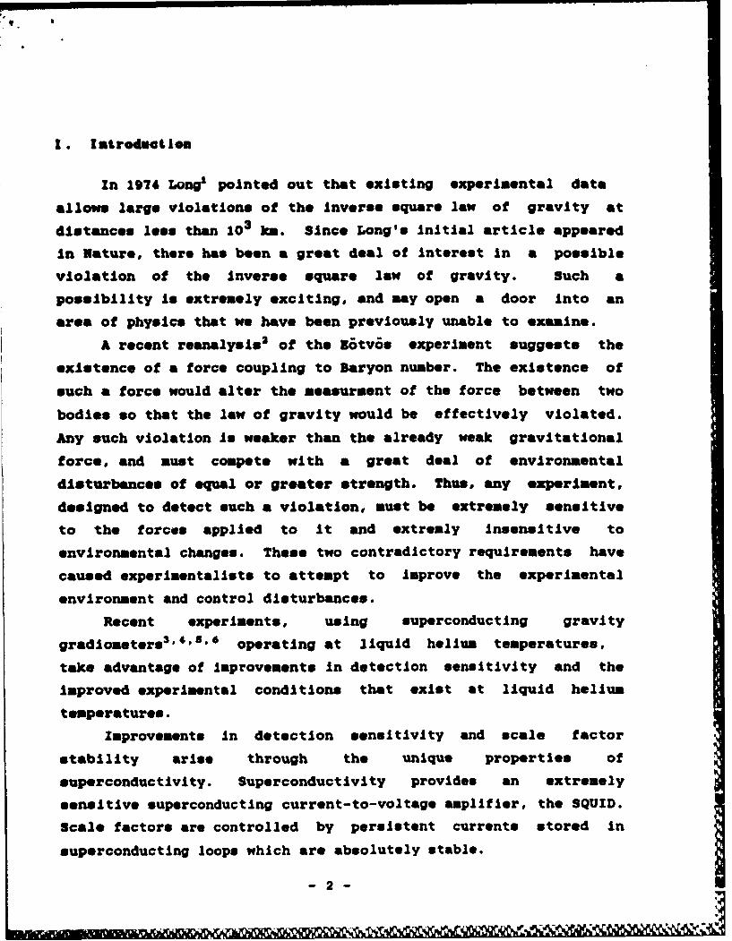
!. lmtroduation

In 1974 Long' pointed out that existing experimental data

allows large violations of the inverse square law of gravity at

distances less than 103 km. Since Long's initial article appeared

in Nature, there has been a great deal of interest in a possible

violation of the inverse square law of gravity. Such a

possibility is extremely exciting, and may open a door into an

area of physics that we have been previously unable to examine.

A recent reanalysis2 of the i6tv6s experiment suggests the

existence of a force coupling to Baryon number. The existence of

such a force would alter the measurment of the force between two

bodies so that the law of gravity would be effectively violated.

Any such violation is weaker than the already weak gravitational

force, and must compete with a great deal of environmental

disturbances of equal or greater strength. Thus, any experiment,

designed to detect such a violation, must be extremely sensitive

to the forces applied to it and extremly insensitive to

environmental changes. These two contradictory requirements have

caused experimentalists to attempt to improve the experimental

environment and control disturbances.

Recent experiments, using superconducting gravity

gradlometers3 '4,' 6 operating at liquid helium temperatures,

take advantage of improvements in detection sensitivity and the

improved experimental conditions that exist at liquid helium

temperatures.

Improvements in detection sensitivity and scale factor

stability arise through the unique properties of

superconductivity. Superconductivity provides an extremely

sensitive superconducting current-to-voltage amplifier, the SQUID.

Scale factors are controlled by persistent currents stored in

superconducting loops which are absolutely stable.

-2-

The experimental conditions that exist at 4 K are vastly

superior to those that exist at room temperature. The thermal

and mechanical properties of materials are much more stable. The

Brownlan motion due to the thermal phonon background is also

greatly reduced.

Despite these advantages and Improvements, superconducting

gradiometers still suffer from environmental disturbances. Three

main types of disturbances are important. Temperature fluctuations

disturb scale factors, change the penetration depth of niobium,

and cause mechanical parts to contract and expand. Seismic noise

partially couples to the differential modes of the gradiometer.

Rotation of the gradiometer introduces centrifugal forces that

must be separated from the true gravitational, or at least

noninertial, forces acting on the gradiometer. Lastly, magnetic

fields can be picked up by the sensing loops in the gradiometer

and amplified by the SQUID, introducing additional fictitious

signals.

All present superconducting gravity gradlometers suffer from

these same noise sources. During 1984 and 1985, we were able to

study these noise sources in the Stanford Gravity Gradlometer .

At the start of this work, excess noise in the low frequency

regime was thought to be due to excess thermal sensitivity in the

superconducting readout circuitry. In order to treat and study

this effect, a second superconducting readout circuit sensitive

only to changes in temperature was added to the gradlometer and

coupled to the readout circuit.

By coupling both the gradient sensing coll and the

temperature sensing coil to the output SQUID, a passive

subtraction of the thermal sensitivity can be accomplished at low

frequencies. At the same time, by storing current in only one of

the sensing loops, thermal or gravity gradient effects can be

independently examined.

3 'A

r r~r . 9 , %, . " . , '--f , w-

4 I

The temperature sensing circuit Is coupled directly to the

gravity gradient sensing circuit through a second transformer.

This change In the readout circuit made It necessary to

recalibrate the instrument. The analysis for the gradient sensing

circuit has been previously done by Napoles' in his thesis. An

extension of this analysis, including thermal effects, is

presented in Section 1x.

During the study of the thermal sensitivity of the

gradiometer, it was determined that two primary sources of excess

noise exist in the gradiometer below 0.2 Hz. These are the

large thermal drift in the readout circuit, and the notion of flux

trapped in the gradioneter and the surrounding shields.

-4-

I1. The Basic Gradlometer

The Stanford Gradlometer4 utlllzes a displacement differencing

method to detect gravitational gradients. The gradient sensing

coil Is rigidly attached to one of the proof masses, and measures

the distance to the second proof mass. By measuring the relative

motion of the two proof masses directly, a partial common mode

balance exists before any of the tuning circuits are activated.

It is this feature that Is the basis of the displacement

differencing design.

The gradiometer is shown schematically In Figure 1. All

parts are cylindrically symmetric. Each of the two proof masses

is supported by two mechanical springs. These mechanical springs

are folded cantilevers cut Into circular disks of niobium and

confine the two proof masses to move along a single axis with a

high degree of mechanical compliance.

When a gravitational gradient Is applied along the sensitive

axis of the gradlometer, the two proof masses move relative to

each other. This notion modulates the Inductance of the gradient

sensing coil which in turn is coupled to the SQUID amplifier which

amplifies this small change in current. The gradient sensing coil

is mounted on the face of m, on a 0.25 cm thick coil form of Macor

machinable ceramic. The sensing coil is wound in a single layer

on the surface of this coil form. It consists of 400 turns of

0.089 mm diameter nlobium wire.

Since the Meissner effect will not allow the magnetic field

from the gradient sensing coil to penetrate the second proof mass

2 , the inductance of the gradient sensing coil may be written as

( 1 ) L a -= A Gd o + A ,, ( x , -X , ) , te

where Ac Is the change In inductance/meter given by Pon2 AG, n. =

-5-

the number of turns/meter, A.- the area of the 6.9 cm diameter

sensing coil, and dc- the effective initial separation of the coil

from the proof mass n2. xi and x. represent displacements of mi

and a2# respectively.

In addition to this modulation of the gradient sensing coil

inductance by the relative motion of m and u2, any change in

temperature will cause a change in the effective spacing, d0 .

This can be represented by a temperature dependent term AOT (T-To)

so that L.19 completely described by

(2) LO - AGdo + A(x 2 -X,) + AOT(T-To)

where AGT gives the change in inductance/Kelvln, and will be

calculated in Section V.

The temperature sensing coil LT was wound as two solenoidal

coils on the outside of the cylindrical casing of the gradiometer.

Each coil has a diameter of 11.43 cm, a width of 2.17 cm, and

consists of 240 turns of 0.089 as niobium wire. These coils are

held in place by a thin layer of Stycast epoxy, and shielded by a

second superconducting niobium shield. Any change in temperature

will cause a change In the effective spacing of the coil to the

niobium casing. The inductance of the temperature sensing coil

can be written as

(3) LT - ATA + ATT(T-TO)

where ATT is the change in Inductance/Kelvin, dT is the effective

initial separation, and AT is the inductance/meter given by

2pon2 AT , where nT - the number of turns/meter of 0.089 mm

diameter niobium wire, and AT - the area of one of the temperature

sensing coils. ATT will be calculated in Section V.

These sensing coils, for gradient and temperature, are

coupled together using two Impedance matching transformers, and

-6-

connected to the rf SQUID as shown in Figure 2. The final

output current containing both gradient and thermal terms is

amplified by the SQUID.

The degree of coupling from the gradient sensing is

proportional to the magnitude of IGO* Similarly, the coupling from

the temperature sensing coil is controlled by . To see this

quantitatively, It is necessary to write three flux conservation

equations, one for each of the loops in Figure 2. These are

(4) (L2 + Le)(IGO+ 0 ) + M2 3 i - (AGdo + L2 )Io0 0

(5) (L3 + L6 + LS)i + M23 (IGO+ iG) + M,6(ITO+ IT) - M23 1GO+ M,5TO

(6) (L,+ L4 )(I.r o + i.T) + Mi I - (AA + L4 )1.ro

where the self-inductances L and mutual inductances NJ are

defined In Figure 2, and 10 and iT represent signal currents for

gradient and temperature. Substituting Eqs. (2) and (3) into Eqs.

(4), (5) and (6), linearizing the equations, and solving for the

output current I, we obtain

M23 IGOAG (x 2 - x 1 )

(7) 1 - +23

(Aod 0 + L s)(L3 + [s + 1,4) - M{2 :3

g 23 IOOAOT

+

(A d + L2 )(L + LS + L4) - M23

}(T-T o )

(A d, + ,)( L + L + L. ) - M, },2,-T., ,

where L- the effective inductance of the gradient sensing coil,

-7

La, as seen through the transformer (L3 , L3 ) by the SQUID, which is

given by12M2

(6) 23(L + Acd )

and L; - the effective inductance of the temperature sensing coil

LT Pas seen through the transformer (L.,L ) by the SQUID, which is

given by

(9) L4 - L5- - Ad(L,+ A^Td )

In examining the output current i, a natural separation of

the two signals, gradient and thermal, can be seen. If we

concentrate on the mechanical motion of the gradiometer, we may

simplify Eq. (7). Ignoring thermal effects, we have

N2 1 0GoA G (x2 - x1 )

(10) i W

(Ar do+ L2 )(L3 + Is+ L4) M123

A gravitational gradient r applied to the gradiometer causes

a displacement of the two proof masses which Is controlled by the

stiffness of the differential spring constant mw. Thus

(1) ix 2 - x1 I b 2 r

where w. is the dlffirential resonance frequency, and b is the

baseline between the two accelerometers.

Thus, when a gradient r is applied to the gradiometer, an output

current ir is produced:

-8-

(12) ir b 3-O(A dg+ L2 )(L 3 + L + - M23

The SQUID amplifies this small current and produces an output

voltage given by

(13) v r - R I r

where R - 2 x 10⁵ 0.

Equation (12) shows only part of the dependence of ir on IGO.

As expected, the differential resonance frequency w. is dependent

on the coupling between the mechanical system and the sensing

cicultry.

A natural measure of this coupling can be given by

2 3

(14) 2 0;2D

where wo is the resonance frequency of the differential mode when

the stored current IGO is zero.

In order to calculate the degree of coupling, 0, and

understand the way in which the sensing current affects the

differential resonance frequency, we must look at the reaction

forces on the proof masses m, and m. due to the magnetic pressure

from the gradient sensing coil. This force is given by

(15) F21 . - A ^o 1 A 1 AG 12 + A i I21GG0Go 0 G GO

where 1o may be calculated by solving Eqs. (4), (5), and (6). We

have

-9-

(16) - A(x 2 - x

L2 * 0 d0) - M /(L 3 + LS +f4Y

where we have Ignored second order terms, and terms dependent on

(T - TO).

Substituting Sq. (16) into Zq. (15), we obtain the force, F21'

of the gradient sensing coil on m2:

(17) 11 - o - - x,)

where

(I8a) 'o " * ~

(lea FO A 120A2I

(lob) 19C n 0

(L2 + A0&a do S/ (L 3 + LS +L4)

We can begin to see the dependence of wo on the degree of

coupling from the gradient sensing coil. The electrical circuit

supplies a DC force which tends to separate the two proof masses,

and an additional spring constant IkE which adds to the mechanical

spring constant. Newton s equations of motion for m1 and m give

for the two modes of the gradlometer

(19a) d (x2 -x() + 2 (x2 -x 1dt2 2 1 a x 1

(19b) t2 (x2 + x,) a (- + (m + x1 )

where M - the mass of the gradiometer casing, k Is the mechanical

spring constant from the folded cantilever springs supporting each

of the proof masses, and m - m W in2 .

The differential and common mode frequency can be seen from

- 10 -

- .'- w~~ g~ EtRfX )--- Wo9 ~ ~ ~ '~ :.~~.

Eqs. (19) to be

(20a) 4U2m~ 2 2 E

(20b) g2 ~~22mWC "0 +R

To complete the analysis, a dependence of k on IO must be

included. This dependence arises through the change in the

equilibrium spacing of the gradient sensing coil, d., as the

magnetic pressure on proof masses a, and increases.

In the Stanford gradiometer, unless the sensing current, IO,

was greater than 4.0 A, the sensing coil and the proof mass m2

touch. Thus for 10, > 1GF - 4.0 A, the gradient sensing coil

equilibrium spacing, do , is given by

(21) do - do + C k Gk

where do - the effective spacing of the gradient sensing coil when

I6 M IOFZGO - GF

Combining Eq. (21) with Eqs. (18) and (20), we may solve for

the complete dependence of 2 on 12

2 A2 x2

(22) c 6 + I GoD 0 A 2W 2

m{A do + 2 + Ok (3 + LS 23+ L )

- 11 -

By setting

(23a) LO a do + L.3 - N 2 3, + LS + L4

A2

(23b) a IaLo (2w) 2

Eq. (22) may be written as

1(2w)2 Y 12(24) Go o 2 I •W., W. + 0 o- 12,,

The dependence of ,2 on 12. can now be seen clearly.

Initially, while 12 : * still small, it is constant at w. As

increases, w 2 climbs to a constant value of 32 for large 12.

This implies that the range of coupling, 0, is 0 to 2/3.

A plot of the experimental data fP versus 12 and a fit to Eq.

(24) is shown in Figure 3. The numerical fit gives

(25a) fo,* 1 p = 68.9 Hz

(25b) -*XP = 31.4 Hz2 /A2

From the geometry of the cantilever springs as given by

Napoles4 and using the classical formula for a bent beam, we have

(26) f2 M 3 Lih l0 T ,t2 (2w )2

where a - 1.07 kg Is the mass of each proof mass, w = 9.55 x

10"3m is the width of each cantilever, h = 7.1 x 1O 4m 1s the

- 12-

thickness of each cantilever, t a 1.115 x 1O-3 is the length of

each cantilever, and 2 - 126.5 x 10P N/m is the Young's modulus of

niobium at 4.2 K. Equation (26) gives

(27) fOLh - 74.4 Hz

This is in fair agreement with f• #*XP" A further check can

be obtained by calculating f. from the fc in Eq. (20b). Using

fc,*XP 0 76.9 Hz, and M - 6.69 kg, we obtain

(28) f• - 69.2 Hz .

This Is In good agreement with fOfexp"

In the previous work with the gradlometer, a f• of 60 Hz, and a

10r - 3.0 A is reported by Mapoles.4 The shift in f• and In I.,

can possibly be accounted for if a shift 1n the equilibrium

position of the springs occurred.

y may be computed from Eq. (23b) by using AG - 0.79 H/m, m =

1.07 kg, do - 250 pm. L2 - 186 pH, ,2 3 - 22 pH, L3 - 4.9 pH, Ls

- 2 pH + 0.6 pH (stray Inductance), and [4 - 0.7 pH. This value

of L4 is computed by substituting L. - 0.8 pH, M45 - 4.4 pH, d =.

19 pm, AT - 2.48 H/m, and L4 - 43 pH into Eq. (9). This results

in a theoretical value for y:

(29) thy - 45 Hz2 /A

Experimentally, we found a smaller number, -rxp 31.4 Hz2 /A2 ,

as given in Eq. (25b).

Now that we have a clear understanding of the mode structure

of the gradlometer and the superconducting readout circuitry, we

are in a position to examine the Intrinsic noise of the

gradiometer.

- 13 -

11. SQUID Amplifier Noise and 3rovnian Notion

If the gradlometer Is operated in a perfectly quiet

environment, i.e., with no seismic noise, no background magnetic

field, and no thermal drift, then the theoretical performance of

the gradiometer is limited by the SQUID amplifier noise and the

noise force coming from the phonon background at 4.2 K.

The SQUID amplifier noise is specified as the equivalent

Input noise energy in J/Hz at the SQUID Input sensing coil L.:

(30) i8 df - , df

where 3 N,s a 6 x 10-29 J/Hz.

This effective noise current at the Input to the SQUID

amplifier is equivalent to a gradient noise, r. ,, acting on the

gradiometer. To see this clearly, we may rewrite Eq. (12) using

Zqs. (14), (18), and (20):

F2 b2 M2 2 m2

(31) 12 a 33

r 413 (L3 + 1.3 +L;) 2 A2

where B is the amplifier coupling as defined in Eq. (14). By

substituting 2 In place of 12 , we may solve for the effective

gradient noise due to the SQUID amplifier noise:.

2 ~~ BA:0 (L3 + 1.3 + 14) 2 EN,(32) r2 df = m df(32) A's m= 2 2 •-

The effective gradient noise due to the phonon background at

4.2 K may be computed from the noise force given by the Nyquist

theorem:

(33)3 df df

-14-

. . -,, .--,ag ' " "'" e # ; ' ' '

This is equivalent to a gradient noise of

(34) r2 df- a dQ

Those two sources of gradient noise give a lower bound on theperformance of the gradiometer:

SA313 (L~ + L + [.4)(35) r2 df Go3W' df + Sk3 df

N oWVM b3' 32 LS b2nQ d

In general, it is necessary to minimize this sum as afunction of I1Go' However, in this case, the amplifier noise is

dominant. The Brownian motion noise may be computed by using T u

4.2 IC, fo a 84 Hz. m - 1.07 kg. b a 3.2 cm. 1k3 n 1.381 x 10²j/X.

Q M ax log:

(36) r WT - 0.068 %/Hz1/2

where 1 E - 1 Zotv6s unit - 109s-2 Is a unit of gravity gradient.

This will be much less than r. , , and we may minimize r. by

Itself* This is equivalent to minimizing

100

This is a minimum when

(38) 1 20 f - 10

Using f0,*,,, - 68.8 Hz and -,, 31.4 Hz2 le , we have IG ,*. -

6.71 A or equivalently, using Sq. (24). we find

(39) 3* 2 or a a 1/3ID 2; opt,

Substituting the optimum current into r. . gives

M 2 1:r)(

( 0 df7r2( j - )arL T- L s+ ;)2 EZR.s

(40) r.d - .*2b2 M23 LSf

Substituting r.xp a 31.4 Hz2 /A2 , fo ,.xp = 68.9 Hz, L3 = 4.9 PH,

L- 2 PH, a - 1.07 kg, b - 3.2 cm, N23 - 22 PH, r - 4.0 A,

R. ,- 5 x 10- 29 J/Hz, and A. a 0.79 H/n, we obtain

(41) F ,,a 2.2 I/Hz 12

Ne may also calculate the scale factor from Eq. (31):

iF b MN 33 0 a(42) - b-23 gr 2I 1 p(L 3 + Ls + 14) As

Using Zq. (13) and substituting in numerical factors, we find

(43) 1 - 0.62 PV/ZF

r,,G is the basic noise of the gradlometer and any additional

noise is due to thermal, seismic, or magnetic noise in the

experimental environment.

For the original Stanford Gradiometer, with a different

transformer, Mapoles4 reported previously that 7 = 70 Hz2 /A2 ,

IGO op&= 4.2 A, and

(44) VE - 1.2 pV/E or F. - 1.14 I/Hz1/ 2

r

This decrease of the gradient-to-voltage scale factor is partially

due to the smaller coupling of the new transformer used In the

present work. However, it does not seem that the factor of 2

-16- " '" "

decrease can be accounted for entirely by this. The most likely

parameter that has changed over 4 years is the coil spacing d0.

Apparently, do has increased from approximately 55 on to 250 am.

This change may be due to a dust particle, or a partial failure of

the epoxy bond that holds the gradient sensing coil to the Macor

coil form. Without disassembly, it is impossible to completely

determine the cause.

- 17 -

111. Gradiom.ter Pertormance

Theoretically, (ignoring environmental noise), the output of

the gradlometer should be white noise at the level of 1.4 pV/Hz1 / 2

from 0.01 Hz to the peaks due to the resonance of the gradiometer

in the common and differential mode. After storing a current

close to the optimum, IGo - 6.69 A, in the gradiometer sensing

coil and balancing the common mode acceleration out of the

differential mode, we obtained the data shown in Figures 4, 5, and

6.

The quietest region occurs Just below 1 Hz with a noise of

approximately 36 E/Hz1 / 2 . This is sixteen times the noise floor

due to the amplifier noise alone, and it must have been caused by

environmental noise. What is even worse is the climb in noise

level below 0.1 Hz since this region is where the inverse square

law experiment is to be performed. In the region where one may

see the signal from the 3.24 x 10 kg steel cylindrical shell, as

It is raised and lowered over the experiment, the noise is

approximately 250 I/Hz1 '2 . This level is unacceptably high, and

must be due to environmental noise, either large thermal drift or.

the movement of flux trapped in the cryostat. The various peaks

seen In the data are caused by resonances in the vibration

isolation used to remove seismic noise from the gradiometer.

- 18 -

IV. Thermal Noise in the Gradiometer

The basic sensitivity of the gradlometer to changes In

temperature is shown in Eq. (7). If we concentrate on changes In

the output current due to a change In temperature, it apprears

that we can slmpllfy Eq. (7) to read

M 23 1 GO GT(45 ) 1 (T - To (

(^od+ LI)(r+ I.S+ LI) -142,

+ M46 ITOATT

(ATdT+ %)(L5+ LS + L ° M 5

This is not correct, it is important to realize that the proof

masses are free to move In response to any change In the

gradiometer sensing current IGO+ 10• A change in the gradiometer

sensing current produces a force

(46) F21 a AG iG IGO

which attempts to seperate the proof masses a distance

(47) x2 - x I G GO

Substituting Eq. (47) into Eqs. (4), (5), and (6), linearizing the

equations, and solving for the current 1, we obtain

-19-

r 2 3 1ooAT --(48) 1 - (T - To ) (1-B)

+ N4 ITOATT4

(ATdT+ L4 )(l+ LS+ LZ') - N2

where L.' is the effective Inductance of the gradient SrAs'j% coil,

when the proof masses are allowed to move, as seen through the

transformer (L. ,L3 ) by the SQUID. Li' is given by

3 k(49) Lo' - Ls - +3 ka

L + A C42. A k ,+ ^Td)(Lg+ L.+ LC - 45

((L4.+ ATdT)(LS+ [6 + L 3 )-M2 5

In writing Eq. (48), we have assumed that the temperature of the

gradiometer is the same everywhere. This should certainly be true

at a low enough frequency. However, we will see that this is not

true above approximately 0.01 Hz. A more accurate assumption is

that each sensing coil has its own temperature; i.e.,

N 2 3M1GoAOT(T - T 0 ) M45ITOATT(TT - TO)(50) 1 W . (1-8) +{Cod + LS2T-3 + 2) = M 3 (ATd+ L4 )(L5 + [-,+ L')

where Ta and TT are the temperatures of the gradient sensing coil

and the temperature sensing coil, respectively.

In examining Eq. (48), is seems clear that the thermal

- 20-

sensitivity of the gradiometer may be "dropped out" by a correct

adjustment of the temperature sensing current, ITO' as a function

of IGO' However, Eq. (50) shows that this cancellation will occur

only at sufficiently low frequencies where T. a TT. At higher

frequencies, a complicated thermal structure will be seen.

At the start of this work, it was felt that the difference in

temperature throughout the gradiometer should be negligible below a

frequency of approximately 0.1 Hz. We have seen in the

experiment, however, that the relevant time scale is on the order

of 100 s. Below 0.01 Hz, Eq. (48) starts to approximate the

thermal situation in the gradiometer reasonably well.

Indeed, the time scales for thermal heat pulses to move

within the gradiometer are on the order of 10 a; however, the

phase shift is still apparent at 100 a. This is because thermal

system are first order in nature.

The gradiometer can be broken up Into several Isolated

thermal pieces. Heat first reaches the outside casing (at Tc with

a heat capacity Cc), then passes to the bulk of the gradlometer

(at T. with heat capacity C.). From the bulk of the gradiometer,

heat moves slowly through the thin niobium springs to the two

proof masses m and m2 (at TN with heat capacity CM), and finally

heat moves slowly through the Macor coil form to the gradient

sensing coil (at T. with heat capacity C.). This is schematically

represented in Figure 7.

The thermal equations of "motion" can be written as

(a) dT P(t) (T¢- T)

dt CC C

dT5 (Ta- Tc ) CC (Ta- TM) CM(51b) - -

dt TcS CS 95 CS

- 21 -

dTM (TM- To )(51c) dt

(5d)dT( (TG- T1)dt ,

where P(t) is heat applied to the outside casing and Tr iS the time

constant for heat transfer from the i-th part to the J-th part.

Using this model, and applying a heat Impulse to the outside

casing through a heater coil, we obtained the parameters given in

Table 1. Typical data and fit to the model are shown In Figures

8 and 9.

A partial verification of these parameters may be obtained by

examining Cc /Cs and CM/CB with an exchange gas pressure

approximately 10-3 p.

Since heat capacity is proportional to mass,

(52) CM mi +m 2 1.07 ka + 1.07 kg 0.32CS + Cc mc + m 6.69 Kg

Similarly from Table 1,

CM C/C B

(53) C - M- 0.35

These numbers are in good agreement.

Using the thermal model of the gradiometer and looking at the

steady state response, we may compute the transfer function:

- 22 -

- -.

(54) T - ToTC

This transfer function will tell us the degree of balance

between the temperature at the outside case and the temperature

at the gradient sensing coil. Setting P(t)/C c m A e'and solving

for the steady state response, we obtain

(5(5) T -

O{CB'FBTcSTNG5 *2 s[TCTN(CN* C ) sN(TNCC + TC )J

+ CC (TBN + TNO )+ (CN+ CS )Tc}

(DTNo+ 1) {CB T N T cea2 + [Tca(cN+ CS) + FBNlCCls + CC)

This transfer function is plotted in Figure 10 for the data with

approximately 10-3p exchange gas. It is clear from the plot that

the temperature of the outside casing and the temperature of the

gradient sensing coil are very different above 0.01 Hz and no

temperature balance is possible above this point.

With a little thought, It also becomes clear that the

temperature of the gradient sensing coil fluctuates much less than

the temperature of the case. At high frequencies, say above

0.2 Hz, all of the thermal noise reaching the case should be much

suppressed when it reaches the gradient sensing coil.

Quantitatively, if we examine the transfer function

-23 -

K b

(56)1

am C5

a IT ca. (TO*.+ No, + T F C.No+ TNTMC 3s[TDN+ TNC+ TC9 ( CM CO + CBI

d;C C )I

it is clear that the gradiometer sensing coil is well filtered by

this third order low-pass function. Substituting in the

parameters from Table 1 for an exchange gas pressure of

approximately 10" p, we obtain

(57) To M _ _ _ _ _ _ _ _ _ _

Tc -jf3 (lgs) 3 -f 2 (46s) 2 +jf(91gs)+1

where we have set a - 2wjf. At a frequency of 0.01 Hz, the

difference between.T. and Tc is only 1.6 db. However, at 0.1 Hz,

TO fluctuations are suppressed by 26 db. This increases to 39 db

at 0.2 Hz. Clearly, thermal fluctuations should make no

contribution to environmental noise in the gradioneter above 0.2

Hz. This is our first indication that the excess noise in the

gradiometer may be due to another source.

By storing currents, I TO - 4.02 A and 1o , 0 A, in the

gradlometer, we can magnify thermal noise and suppress Inertial

disturbances. This data Is plotted in Figure 11.

Comparing this with our previous data in Figure 5, we see

that our excess noise above 0.2 Hz must be related to Inertial

disturbances. This comparison is shown more clearly in Figure 12.

Below 0.2 Hz, the excess noise may be due to the movement of

magnetic flux trappped in the shields surrounding the gradloneter,

-24-

or due to fluctuations In temperature. Inertial disturbances

should be somewhat suppressed below 0.2 Hz since, In this region,

seismic disturbances drop In amplitude and there are no resonance

peaks in the gradiometer suspension structure. This drop in

amplitude, which Is measured with a room temperature accelerometer

constructed at the University of Maryland, is shown In Figure 13.

At worst, the seismic noise should provide a flat background, and

yet we observe a sharp Increase as f becomes zero.

If we examine the output of the gradiometer without any

current stored in the readout circuitry, we obtained the data in

Figure 14. We observe a large amount of excess noise. This noise

cannot be caused by temperature changes in the gradiometer, as the

amount of residual current trapped in the gradiometer is very

small. Typical data for the gradiometer ouput voltage, with no

current stored, is plotted as a function of time, is shown in

Figure 15. Flux movement is shown clearly in Figure 15.

The type of step function, as shown In Figure 15, will produce

noise with a 1 /fa characteristic when it is spectrally decomposed.

This noise will contribute to the excess noise in the gradlometer

below 0.2 Hz. By comparing the data in Figures 14 and 11, we

conclude that, while the movement of flux is important, it is not

the major source of noise below 0.2 Hz. Adding a p-metal shield

to the dewar would eliminate the low frequency noise due to the

movement of trapped flux, but excess thermal noise would still be

present. The flux noise is, however, very important in any

experiment in which the signal frequency lies above 0.1 Hz.

Mapoles' previously reported a thermal sensitivity of the

gradiometer, dV/dT, equal to 31.6 x (Io/ 1 A) V/K . This is an

extraordinary sensitivity to temperature changes. If the

gradlometer has 6.69 A stored in the gradient sensing coil, It is

necessary to stabilize the temperature to better than 6.6

nX/Hz 1/2, over the region of experimental interest, in order to

- 25 -

. .h.-n . .

limit the contribution of thermal noise to the total noise so that

the SQUID amplifier noise dominates.

By adding the readout circuit sensitive only to changes in

temperature, it was hoped that a passive subtraction of temperature

changes could be attained for frequencies below 0.1 Hz. We found

that this subtraction did not occur until approximately I mlz. At

this frequency, we did observe much Improvement in the thermal

sensitivity of the gradiometer.

-26-

- .26 - .1i

V. Thermal Sensitivity in the Gradlometer

During the original work on the Stanford Gradiometer, the

only candidate for the mechanism that produces the high thermal

sensitivity of gradiometer , dV/dT, wan the change in the

penetration depth of niobium as a function of temperature. This

effect was 10 times too small, and the actual mechanism was

unknown. Whatever the mechanism, it was thought that it should

decrease as the temperature was lowered below 4.2 K. Napoles

constructed a cold plate in order to cool the gradiometer. This

did not, however, improve the thermal performance.

We now know that three major mechanisms affect the thermal

sensitivity of the gradiometer. These are, the change in

penetration depth of niobium, the thermal expansion of Stycast epoxy

at cryogenic temperatures, and the change in Young's modulus of

niobium below the superconducting transition point.

For the first effect, Mapoles' reports that

(58) dA(T) 2%o _) T )1-3/2

dT TC TC ~TC

where X 440 A and Tc - 9.2 K for niobium. At 4.5 K,

(S9) dX(T) . 1.22 x 1- 9 m/KdT

It is difficult to determine the thermal expansion

coefficient of Stycast epoxy at 4.5 K, but an estimate may

be obtained from Serafinl and Koenig of

dL(60) f1.5 x 1i0 /K

L dT

- 27 -

The change in Young's modulus of niobium as reported by

Kramer and Sauer9 is dependent on the degree of stress In the

sample, the degree of chemical purity, and the frequency at which

It Is measured. A rough estimate of this appears to be

dY

(Sla) .1 - 25 x 10 /K at 4.5 KY dT

(Gib) IdY

( Sib)50 x 10- 6 /K at 3 K and belowY dT

These three effects can be used to compute the expected change

In self-inductance of the gradient sensing coil and the temperature

sensing coil.

The temperature sensing coil Is shown schematically In Figure

16. The thickness of the layer of epoxy bonding the niobium wire

to the niobium casing of the gradiometer is approximately 130 pm.

If we assume that the wire moves half the distance that the epoxy

expands or contracts, then the change In the coil spacing may be

computed as

d =T 1 dL(62) [ }65P Px - 0.98 x 10 - 9 m/K

dT epoxyLdT

The change In the penetration depth of niobium contributes twice,

once at the surface of the wire and again at the surface of the

casing. There arises, however, a factor of one half which cancels

this. The pentratlon depth is defined as the mean distance over

which the magnetic field B penetrates a superconductor. If BO is

the field strength at the surface and B(x) is the field strength

Inside the superconductor, then

-28-

(63) 5(x) U so* -

The amount of magnetic energy that penetrates the inside of the

superconductor per unit area is equal to

x6f I B2 "-2x/(T) dx - X (T)(64) f ;,L4fl. - 0TP

0 0

The resulting change in self-inductance effectively modifies dT as

(65) - 2 x 7x d)(T) = 1.2 x 10 -9 n/KdT J dT

The change In dT due to penetration depth changes and thermal

expansion add together to give

(66) - 2.2 x I0 -9 M/K

total

ATT can now be computed by setting

(67) ATT - AT X w 2.49 H/m x 2.2 x 10 9 m/K - 5.5 nH/Kd total1

The gradient sensing coil is shown schematically in Figure

17. The sensing coil is held to the Macor coil form by a thin

layer of Stycast epoxy approximately 125 pm thick. This Macor

coil form is held to the proof mass m by a second layer of

Stycast epoxy approximately 25 pm thick.

- 29 -

Because the thermal expansion of the epoxy moves the sensing

coil and the coil form towards the proof mass ml, the equilibrium

spacing do is reduced. As previously, we assume that the niobium

sensing coil moves half as much as the expansion of the epoxy

bonding it to the coil form. To this is added the expansion of

the thin layer bonding the coil form to the proof mass a2 . The

expansion of epoxy gives,

(68) 4T] -- (65 pm+ 25 pm) x1 d - 1.4 X iV i/KL dT

The change in d. due to penetration depth changes is

identical to the change in dT#

1r

( = 2 x 1x dLl T + 1.2 x 10 9 m/KdT J dTL ponetrotlon

At this point, we immediately notice that Eqs. (64) and (65)

almost cancel each other. Thus, without a third mechanism to

provide additional thermal sensitivity, there is no hope of

explaning the large thermal sensitivity of the gradiometer.

This third mechanism is provided by the niobium springs that

support the proof masses. Because the Young's modulus changes as

a function of temperature, the equilibrium spacing d. fluctuates

with temperature.

The sensitivity of the gradlometer output to this change is

directly proportional to how much the springs are loaded. To see

this clearly, we may compute the equilibrium spacing of the two

proof masses. The magnetic force causing the masses to separate

is

- 30 -

&•".A -AC PA.. . . . . . , .. ,. . / .. .' ' '

(70) B27A 71 2IG

This defines the equilibrium stretch d.ST Setting the

restoring force equal to the magnetic force, we obtain

(71 49 T - A 12

where the factor of 2 enter* because both proof masses Rove.

Solving for d8Te we find

A0 1 2(72) doT FG

The mechanical spring constant k is directly proportional to the

Young's modulus of niobium. Differentiating d. with respect to

temperature, using Eq. (25) and setting k - mw;, we find

] AI 12 dYrd~ddT -- Mri2 Y dT dTJ

sopring spring

Setting A. 0.79 H/m. a - 1.07 kg, f0 *XM 68.9 Hz, 1I pot

6.69 A, and using Eqs. (61) , we obtain:

(74a) d d1o 4.4 x 10⁻⁹ r/K at 4.8 KdTJId pri ng

(74b) ( d G . 1- /K at 3 Kand belowI d sopri ng

- 31-

In contrast to the change in penetration depth, this effect is much

larger at 3 K than at 4.5 K.

Equations (68), (69), and (74) combine to give

(75a) -dd - 4.6 x 10⁹ r/K at 4.5 KdTJ

(75b) [do...] 9.0 x 10⁻⁹ r/K at 3 K and belowdT

AGT can now be computed by setting

(76) A T A . x ,

substituting in Eqs. (75) and setting AG = 0.79 H/m, we obtain

(77a) AGT - 3.6 nH/K at 4.5 K ,

(77b) AGT - 7.1 nIH/K at 3 K and below.

di/dT for the gradlometer may now be computed.

Differentiating Eq. (48) with respect to the gradient sensing coil

temperature and the temperature sensing coil temperature, we

obtain

(78a) - dia - (1-0)0 (A d + L2 )(L3 + LS + ) - M333

- 32 -

(78b) I di L)(T. TT L ') - M

ITO aT (A~dr 12- 04

By Substituting, Eqs. (67) and (77), and other numerical

parameters into these equations, we obtain

(79a) 1 di - . 05A at 4.5 K

(79b) 1 l 4.0Ox 105 /K at 3X and below

(80) 1 di - 3.7 x 10- /K at 4.5 X

gsing Eq. (13), we can calculate the corresponding change in output

voltage:

(81a) [a. R 100 . - 4. 0 V/K at 4.-5 K

(b)(aT. 0)mRIG 7 8.0 V/K at 3 K

-33-

(82) aTT R 1 aT .4 V/K at 4.5 K

Experimentally, we found

(93a) (TO3 q - 30.0 V/K at 4.5 K

(84) IST] 17.5 V/K at 4.5 K

Hapoles measured previously

(83b) Fa3 43.6 V/K at 2.4 K

Comparing Eqs. (84) and (82), we find that the experimental

value is twice as large as the theoretical value, and our rough

estimate for the expansion of stycast epoxy at 4.5K must be too

small by a factor of two.

Comparing Eqs. (83) and (81) we find that the experimental

value is much larger than the theoretical value. The change In

Young's modulus ,as reported by Kramer and Bauer' *Is stronglydependent on the chemical purity and the degree of stream In the

sample. It is also dependent on the frequency at which It 1*.

-34-

A~~~ .:11111I 61.

measured. Kramer and Saue report dY/dT for 80 kHz and 240

kI~z. The value at 240 kliz is approximately half as large as that

at SO kilz. Perhaps It is reasonable to suspect that dY/dT is 2 to

3 times larger at 70 H~z. If we substitute

(I5 dT 75 x10- /K at 4.3 K

anid use a thermal expansion coefficent for stycast epoxy that Is

twice as large, I.e.

1dL -(66) - - 3.0Ox 1O /K

L dT

we obtain:

(67) T 12.7 V/K at 4.5 K.[ )t. hy

This is still too small.

Experimentally, dV/dT. Increases below 3.0 K. This is evidence

that our understanding of the thermal properties of the

gradiometer is basically correct.

35

VI. Conclusion

At the start of this work, excess noise In the low frequency

regime was thought to be due to excess sensitivity to thermal drift

in the gradient sensing circuit. We have confirmed this for

frequecies below 0.2 Hz. At higher frequencies, we have shown that

there should be no contribution from thermal drift.

Previously the large sensitivity of the gradiometer to

thermal drift was not understood. We now understand that this is

primarily due to change in Young's modulus of niobium with

temperature.

In addition to the noise generated by the thermal drift at

low frequencies, we have also found that the motion of flux

trapped In the lead shield surrounding the gradlometer leads to

noise with a 1/fa characteristic. The addition of a p-metal

shield to the cryostat would remove this.

We have demonstrated that a passive subtraction of the thermal

sensitivity can be accomplished at low frequencies. This

subtraction can be extended to higher frequencies by coupling the

temperature sensing coil more tightly thermally to the gradient

sensing coil. This could be accomplished by mounting the

temperature sensing coil to the inside surface of the gradient

sensing coil form. This would minimize the thermal time constant

between the gradient coil and the temperature coil. It is believed

that such a geometry would allow cancellation at frequencies below

0.1 Hz. This combined with conventional temperature stabilization

of the inner vacuum can would allow the inverse square law test to

be carried out.

Another way of reducing the temperature sensitivity of the

Stanford Oradiometer is using a current-differencing scheme employed

In the gradiometer developed at the University of Mayland6 . In this

device, the displacements of the two proof masses are sensed by two

-36-

A

:-,

separate sensing coils, each mounted on the same side of the

respective pratt mass. A temperature change now produces efftects

which look like a comazon acceleration and are therefore rejected byI

the common mode balance of the two sensing loops.I

-37-

Ackunowledgement

We wush to acknowledge the valuable contributions by Dr. Mike

McAshan.

- 38-

REFERENCES

1. D. R. Long, Nature 260, 417 (1976).

2. 3. Fishbasch, D. Sudarsky. A. Szafer, C. Talmadge, andS. R. Aronson, Phys. Rev. Lett. 56, 3 (1986).

3. H. A. Chan, Ph.D. thesis, University at Maryland, College Park.Maryland (1962). unpublished.

4. 1. R. Mapoles, Ph.D. theass Stanford University, Stanford,California (1981). unpublished.

5. H. J7. Paik, J7. Astronaut. Sci. 29, 1 (1981).

6. H. A. Chan, N. J7. Paik, N. V. Moody and 3. W. Parke,IEEE Trans. Magnetics, HAG-21, 411 (1985).

7. Model 330 RI SQUID system, Diozagnetic Technologies. Inc.,San Diego, California.

8. Serafini and Koenig In Cryogenic Properties of Polymers.

9. 1. J7. Kramer and C. L. Sauer, Phy. Rev., 163, 407, (1967).

-39-

N 111 1110 1 !1! 1 11

Table 1.

Presure cc /C cm /CB Ir am~ co~ T G

S10- p 0.73 0.60 6.3 a 0.46 0 5.24 a20 p 0.67 0.96 1.1 a 0.13 s 1.37 a

100 p 0.47 1.5 0.99 a 0.43 a 0.69 a

-40

mo-.0I 0

doo

Eor

c3 J7

4 -.-...

t I

tm~

qqD

SI'

I-iS

U

~4C

(%y#)

C

DCVI

K

ft.

I

I -F

41

. . . . . . .. ...

LA I 't ,i,.

.9 . 0

(A'I . I I 'I t

I * . III I

* *1 I* I2 a 1***~~ -*-i-* .1

'~ ~L S I i a

-- Ia I I .1I I I I

I .. :I * S a * M7s.~-.

I .

-- ~&'~~O- 0 ? dEb~~p~q~ .;~j~: a I -I I I9 a I I . a 4 I a

____ a 5 9 1L J 1 I:

-I *f** f I.......-.-- I a ~~I

I ~-***----**-~*! at aI - U

* j . ~ ,. *1*I

I * a 4 ~ .

-- I a

I I I I I7.I I ( I 9 a a . . a a,

* 9 a

, 1 71r- __

-Ht---i___ -

___ I __

~S J4.~~A.~*~b* J. .~: ~

II.

jjvt.:4 9 a'

PIN

. ... . . . .. . . .. . .

. .. ... ..... .. ... .. 7

. _.. . .. . .

oL~ts;&~~ Liheco4er RPCCT

Rfce

(J1,t-m3. CM

Macor V, C

F~ure7 Tlevrd V, meI

Ap

* ~~~~~~~ ~ ~ j 4 1U ,i. ** ****. . , .

- . -* .~ -h.--~4 .f ~ . ...a ~j~ -.- 4 L

i.~I.. a.(ON

17 * . . * .

*1P. - .

FTTFTTTTmT.TTTT J - ~JT - L...J 7TTFT~

-' I.-.±----...,

* 'AL. ~' 111111 sj....:.~ -1hC ~ i~~I V.'

t~Ii7I 4 J I I .. . . & A'-- I I .-.-. --I-~I-------- -~ c9I I

. I I * I.8

~

* *

. ..... ~ jf *1 I-a4 .4 *

* :. . .1 *1--- - - - ---.--.- .---.-. .- .-----. ,----.** .------------- --

7 K.- SI1.

U* -.. -.. . . -.- -- 3~~~ -. -.-

(. . ~. .

.4

I-

±

g~Lr~

I . I I

( -II I . p

~ z~z z.. I *

'. -. . -. - --.- ' : r , - -:\ , , - , .... .. .. ...... . .. .T... .... 4" " ..." . :. " .'

... . . i .. I" ' I t ! I ;" Ii : 1 .*

!,..i°. -....

S. - - . - . . ' . .I i\--i . . .i . : - . -i q .'- .

• ,..: \ . , -.i .: .

•-|. .. ,E. .. . . . I. . . .

" - . . - . .. . . ..- .. ...- ..... ...... -

"C .. .. i .

.a:..? . . f

II

-- '

.. . ... . . . .. . - -I ,

. . . . . . .. . . . . ..4 . . . _

T -~ T ~ ~~1-*1.

I. .

-4

I ~iI - .

H ~4i L 4- -L:~I--t-i ~ :.

.

. . I

.a.-.

K <~- 2* . I ~*'~ .:I

I

..

* 4

* a a

--- -.-- w.. .~ .---- ~J- - - --

a a a

- -a--.- -.- .9 -a-

- -t

a I

aI . . I I

te~ -I-

-I---~- - ~~1~~~

I.

:.4

I I I ~ . ..

a .~ ~jj .:1:4:>

-- - -

-~

.1 .. I -

7 t .j:. i I-I- I .7I:

~ * j..

1!Ta

~T. 9:

* .

. *

* a --- :1--

____

::I..>.......-. ______ -.

- -~- ~-

I . i . j .. a..

-.

.aI a

* . a I

IZYIIIIIILIZ I>" *1-

I I

a * .

I--a

.' * __ -.

___ ____ I ~ C

I-- ______

I..... -~ -

............. *1i 1 ~*

1 _________

a.

-

V

~iI-i * - 1~ Ti771~

<1 Pa. %aJI. %a

f~I~ I- T~1~I

I -I t~-.-J-.

*. ... .... ..~

-~~~ 75)- - -

.. ... ...

E ** -

20

2

d.

j

V -

I iI~

1- -4---4--I- ... ~L NI . I I I . I . .1* ____

I I .jI 0

I *~ .......!........ - ~0~ - -

- - I I I Ir-r

* I I. I I -3~ I . * -I

.1 0 * * 4 .

C * 0

* . I-- *

9 .0-. .--.-..-- . ---.3 - .. - -. --

I 0 0 Ig1 0 . 0~. 0

-i- - ... L* * I I --

* :. **i*~** ~ 0 .j.: .~

* I . . . . S* . . *9 0

- -- ~

o . I *_____ * . 0 - - - 0

* . . .9

I. * 4 . a

~1 0

- __ __ - -I- -.- - - -* . 0

£ .* j. * .l*; I

.3 d -~ Th -" ~ -

I

*1 :. ___ jj*~ *I*--**-- 1

_ __I ____ ____ -

) F I jI I

-. 9 _____ ____ _____

*.. _______

I II . -

_____ ______ _____ _____ I _____

* 0. 1=-i I--.I E~±~ii L.

0~*

19

-~4-~-.-h~-~ 0

.0~* ~

777 : .....- -

--, i I

I ....... .. . . L4

-. - -- ' - ' ' - I -- _r ,

.. . ' . . ... .. ,

] ." .... .' .. ... ... . .. .. -_

I A M -

_..4 .......

. ..._ ... . ....... L. .

, , I _ > -T .. i ....

'~~- ---- .- :"- _ " . -.i' -!: -

• • 1 -

_ _ _.'_".__'": . . .r-" : ' .. .: '

. . .. . . .I.. . - " . .. : -- -: : "i"'. ...:1 .

t '"" .. . .... ..- i t . :: .-.

• " " •4. I .. ....

. ....,-.,-:' :. _

.. ....J! -

, . . .S... ... ....., - ... . . -S .. I-i. . .. - " -

" t i" ! I ! . -i-1:... 1 !.iL _:

-' I' -. ...-..] .-.I~

-- i--- ' ___i --; ...V E-,: i :!: . I. 1

.... ... .. i IS

OCOo 0cO Epoxid

R re 16 Ternper-*oce Sensur Co011

moiom mm

100 00

o0000<

'

tnob'imw re M Icc ocI l

41 q - -

Q% IL E

Fiaurz 17 ymacIevlt Seiasfl O

lilip


Recommended