Thermal ratcheting of a P91 steel cylinder under an axial moving temperature distribution M. E. Angiolini a, G. Aiellob, P. Matheronb, L. Pillonia, G. M. Giannuzzia

a ENEA Via Anguillarese, 301 - 00123 Rome, Italy b CEA Saclay, F-91191 Gif sur Yvette, France Abstract The progressive inelastic deformation, commonly referred as ratchetting, is a major concern in the design of components and structures submitted to mechanical and thermal cyclic loads in the plastic range. In the RCC-MRx code, the design assessment against ratcheting is performed by applying a simplified method based on the elastic analysis of the structure. The design rule uses a diagram, called efficiency diagram, elaborated essentially on the basis of the results of tension/torsion experiments. In this work the application of the RCC-MRx efficiency diagram to P91 steel has been investigated. It has been considered the thermal ratcheting of a cylinder subjected to a moving axial temperature gradient with no primary stresses applied. The thermal loads have been produced via hot liquid thermal shocks, by dipping a cylindrical mock-up in a molten eutectic mixture of sodium and potassium nitrates. The experimental results show that the present efficiency diagram in RCC-MRx is not suited for P91 steel. Its use for the design would foresee cumulative strains lower than those observed experimentally which is clearly not conservative. This result confirms the results obtained in previous tension-torsion ratcheting tests and provides additional data for the development of a modified efficiency diagram suited for 9Cr steel. 1. Introduction Modified 9Cr 1Mo steel, designated T/P91 steel, was developed during the 70's and has been used extensively in the power generation industry due to its excellent mechanical properties. In recent years, P91 has been considered for use in several proposed Gen IV reactor concepts for out-of-core (pressure vessel, piping, etc.) and for in-core (cladding, wrappers, and ducts) components due to its excellent resistance to radiation damage [1,2]. P91 presents high yield strength, low thermal expansion coefficient (at least 30% lower than austenitic steels) and high thermal conductivity. This makes it extremely resistant to thermal loads and thermal fatigue. On the other hand, because of its softening behaviour under cyclic loads, P91 is known to exhibit “material ratcheting” i.e. accumulation of plastic deformation [3,4]. Ratcheting occurs in structures submitted to cyclic loading in the plastic range with a non-zero mean stress (primary or secondary). It is a phenomenon determined by both the inelastic behaviour of the materials and the behaviour of the structures considered. Even for structures that are designed to behave in the elastic regime, plastic zones may exist and under certain combinations of the primary and secondary loads, under cycling, there may be accumulation of plastic strain with increments at each cycle [5]. In the RCC-MRx code, the design assessment against ratcheting is performed by applying a simplified method based on the elastic analysis of the structure. The design rule uses a diagram, called efficiency diagram, elaborated essentially on the basis of the results of tension/torsion experiments. It consists in determining an effective primary stress Peff which, if applied alone in the same condition of time and temperature, would lead to the same accumulated strain obtained by the application of a constant primary stress P combined with the cyclic secondary stress. The efficiency diagram given in the RCC codes has been constructed and validated starting from a considerable number of results of experimental tests performed on austenitic stainless steels. With

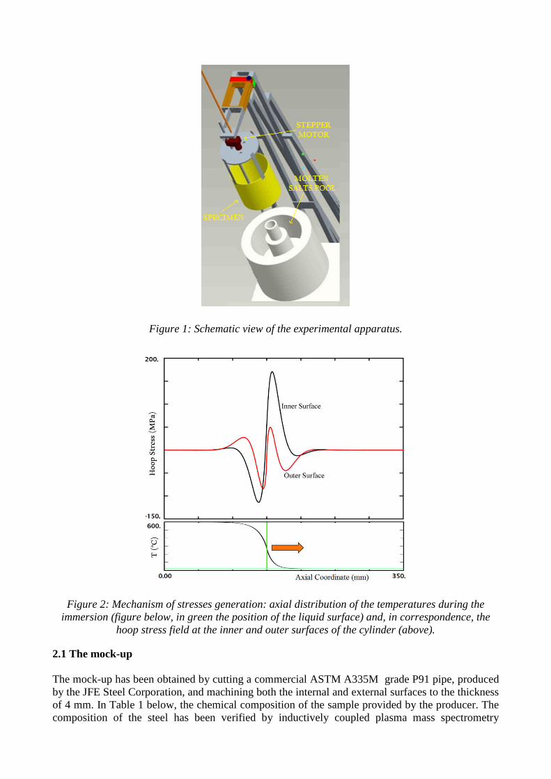
respect to the austenitic steels, 9Cr 1Mo steels, as well as the other ferritic/martensitic steels, present a very limited strain-hardening capability and soften under cyclic loads. So the application of the efficiency diagram for the analysis of T/P91 components requires the evaluation of the present rule and eventually the development of a modified efficiency diagram to take into account their specific behaviour. Objective of this work has been to provide experimental data for verification of the RCC-MRx ratcheting rule for P91 steel. It has been considered the situation representative of the ratcheting due to the variations of the free level of the coolant on the reactor vessel of a molten metal reactor: during the operation the coolant level moves up and down cyclically and the walls of the reactor vessel are cyclically subjected to a travelling axial temperature distribution. The stresses exerted on the structure are mainly linked to the movement of the axial thermal gradient since at the free surface the primary stresses are low or negligible. However, despite the absence of primary loads, there is a risk of progressive deformation [7,8,9]. This is a known problem and in the past, many studies and experimental programs have been undertaken in order to find reliable methods of structural analysis directly applicable to this specific case, where the primary type stresses are null or negligible [10,11]. These studies led to an improved design rule in RCC-MR and to the application of a simplified analysis based on the calculation of the primary stresses not only on the basis of dead weight, pressure or moment loads but also taking into account that a fraction of the secondary membrane stresses acts as a primary stress [12,13]. This work is part of a more general experimental campaign carried out in the frame of the FP7 MATTER Project for the assessment of the design rules for P91 components. Experiments in support of the development of an improved ratcheting rule have been performed by means of tension-torsion ratcheting tests performed on P91 tubular specimens and reported in P. Matheron et al. [6]. Tension-torsion experiments and the thermal ratcheting tests, presented in this work, both indicate that the present rule for ratcheting is not conservative and predicts cumulative strains lower than those observed experimentally. A modification of the efficiency diagram rule of the RCC-MRx code is necessary in order to take into account the specific behaviour of 9%Cr steels. 2. Experimental part To represent the problem, it was chosen as model an hollow cylinder subjected to a thermal gradient with axial symmetry cyclically varying with time and no primary loads applied. The thermal loads have been produced via hot liquid thermal shocks by dipping, with a speed of 1 mm/s, a cylindrical mock-up, with an external diameter of 406 mm and thickness of 4 mm, in a molten eutectic mixture of sodium and potassium nitrates (NaNO3 60%-KNO3 40% melting point at 221°C and stable in air up to 600°C) at 570°C. After each thermal shock the mock-up was extracted from the molten salts pool and cooled to room temperature. A schematic diagram of the experimental facility is given in Figure 1. The mock-up is mounted on a metallic frame equipped with a stepper motor that makes possible to move it along the vertical direction with careful control of position and speed. The specimen speed during the immersion, the temperature of the molten salts and the thickness of the mock-up have been optimized by FEM simulations in order to approach the combination of variables that maximize the hoop stress. During the immersion, a temperature field with axial symmetry travelling upward is generated and, in correspondence, each point of the cylinder experiences a tensile hoop stress field before the contact with the liquid surface followed by a compressive hoop stress field when it gets below the liquid level (Figure 2).

Figure 1: Schematic view of the experimental apparatus

Figure 2: Mechanism of stresses generation: immersion (figure below, in green the position of the liquid surface

hoop stress field at the inner and outer surfaces of the cylinder

2.1 The mock-up The mock-up has been obtained by cutting a commercial by the JFE Steel Corporation, and machining both the internal and external surfaces to the thickness of 4 mm. In Table 1 below, the chemical composition of the steel has been

Schematic view of the experimental apparatus

Mechanism of stresses generation: axial distribution of the temperatures , in green the position of the liquid surface) and, in correspondence

at the inner and outer surfaces of the cylinder (above)

up has been obtained by cutting a commercial ASTM A335M grade P91 pipeand machining both the internal and external surfaces to the thickness

chemical composition of the sample provided by the producerhas been verified by inductively coupled plasma mass spectrometry

Schematic view of the experimental apparatus.

temperatures during the and, in correspondence, the

(above).

ASTM A335M grade P91 pipe, produced and machining both the internal and external surfaces to the thickness

provided by the producer. The inductively coupled plasma mass spectrometry

analyses. The height of the sample has been fixed to 410 mm in order to have a wide region along the vertical axis where the distance from the top and bottom of the sample was larger tlength L of the thermo-elastic stressesformula [14].

L = π /β with

where Rm is the mean radius, t is the thickness andThe sample has been instrumented (external surface along the axial directionthe mock-up to 200 mm and at Diametrically opposed, along the axial direction have been bottom and at 100 mm, 150 mm, 200 mm and 265 mm to check the axialtemperature field. Element C Si Mn P

% 0, 1 0,26 0,41 0,018

Table 1: The chemical composition

During each thermal transient the temperature data have been recorded every 0.2 sec by aspeed data acquisition system. 2.2 Strain Measurements The measurement of the deformations required to dismount the sample from the frame and the acquisition of its profile with a scanninguses a water coupled ultrasound transducervertical direction, to acquire the distance from the sample's surface. rotating platform that allows to performis 10-3 mm for the radial measurement (distance from the transducer), an error of 0.1 mm for the axial repositioning and an error of 0.1° for the disk rotation. circumferential points for 400 circumference scans along the vertical direcSince the distance measured by the ultrasound sensor at each point is relative to the position of the mock-up on the rotating table, different error in the measurements made of a periodic component with period 2component of the error has been eliminated by averaging the circumferential measurements

The height of the sample has been fixed to 410 mm in order to have a wide region along the vertical axis where the distance from the top and bottom of the sample was larger t

elastic stresses, that has the value of 69 mm, calculated according to the

(1)

is the mean radius, t is the thickness and ν is the Poisson's ratio. The sample has been instrumented (Figure 3) with 16 k-type laminated thermocouples

axial direction: on one side about every 50 mm from the bottom edge of to 200 mm and at 110 mm, 160 mm, 210 mm, 265mm, 275 mm

Diametrically opposed, along the axial direction have been placed 5 thermocouples, one at the at 100 mm, 150 mm, 200 mm and 265 mm to check the axial

S Ni Cr Mo Al Ti V 0,003 0,19 8,54 0,86 0,002 0,001 0,198

: The chemical composition of the material used for the experiments

Figure 3: Thermocouples scheme

During each thermal transient the temperature data have been recorded every 0.2 sec by a

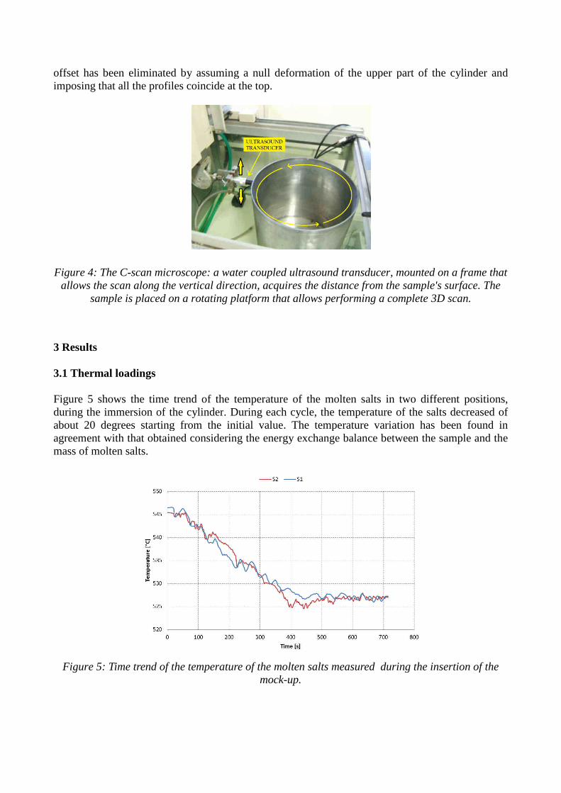
The measurement of the deformations required to dismount the sample from the frame and the scanning ultrasonic water-jet probe C-scan.

ultrasound transducer, mounted on a frame that allows the scan along the acquire the distance from the sample's surface. The sample is placed on a

perform a complete 3D scan (Figure 4). The precision of the system mm for the radial measurement (distance from the transducer), an error of 0.1 mm for the

axial repositioning and an error of 0.1° for the disk rotation. During each measurement 72 circumferential points for 400 circumference scans along the vertical direction have been acquired.

he distance measured by the ultrasound sensor at each point is relative to the position of the ifferent positioning of the sample on the rotating table introduce an

ade of a periodic component with period 2π and an offset. The periodic component of the error has been eliminated by averaging the circumferential measurements

tRm/)1(34 2νβ −=

The height of the sample has been fixed to 410 mm in order to have a wide region along the vertical axis where the distance from the top and bottom of the sample was larger than the decay

, that has the value of 69 mm, calculated according to the

thermocouples placed on the about every 50 mm from the bottom edge of

275 mm, and 350 mm. 5 thermocouples, one at the

at 100 mm, 150 mm, 200 mm and 265 mm to check the axial-symmetry of the

Nb N Zr 0,074 0,0383 0,005

of the material used for the experiments

During each thermal transient the temperature data have been recorded every 0.2 sec by an high

The measurement of the deformations required to dismount the sample from the frame and the . The C-scan apparatus

t allows the scan along the The sample is placed on a

. The precision of the system mm for the radial measurement (distance from the transducer), an error of 0.1 mm for the

During each measurement 72 tion have been acquired.

he distance measured by the ultrasound sensor at each point is relative to the position of the positioning of the sample on the rotating table introduce an

and an offset. The periodic component of the error has been eliminated by averaging the circumferential measurements. The

offset has been eliminated by assuming a null deformation of the upper part of the cylinderimposing that all the profiles coincide at the top.

Figure 4: The C-scan microscopeallows the scan along the vertical direction

sample is placed on a rotating platform

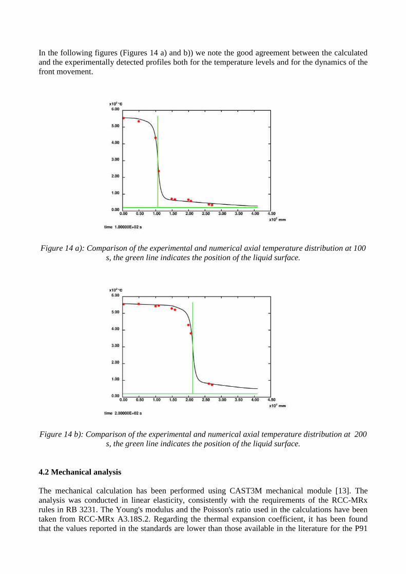
3 Results 3.1 Thermal loadings Figure 5 shows the time trend of the temperature of the molten salts during the immersion of the cylinderabout 20 degrees starting from the initial value. The temperature variation has been found in agreement with that obtained considering the energy exchange balance between the sample andmass of molten salts.

Figure 5: Time trend of the temperature of the molten salts measured during the insertion of the

offset has been eliminated by assuming a null deformation of the upper part of the cylinderimposing that all the profiles coincide at the top.

microscope: a water coupled ultrasound transducer, mounted on a frame that allows the scan along the vertical direction, acquires the distance from the sample's surface

rotating platform that allows performing a complete 3D scan

shows the time trend of the temperature of the molten salts in two cylinder. During each cycle, the temperature of the salts decreased of

about 20 degrees starting from the initial value. The temperature variation has been found in agreement with that obtained considering the energy exchange balance between the sample and

Time trend of the temperature of the molten salts measured during the insertion of the mock-up.

offset has been eliminated by assuming a null deformation of the upper part of the cylinder and

mounted on a frame that from the sample's surface. The

allows performing a complete 3D scan.

in two different positions, each cycle, the temperature of the salts decreased of

about 20 degrees starting from the initial value. The temperature variation has been found in agreement with that obtained considering the energy exchange balance between the sample and the

Time trend of the temperature of the molten salts measured during the insertion of the

Figure 6: Time trend of the temperature of the mock

Figure 6 reports the plot of the time trend of the temperaturethermocouples located at different distances from the bottom of the sample. The thermocouple labelled F1 is located at the bottom and tFigure 3. The recordings show that the temperature at which the contact with the salts takeincreases due to the heat diffusion in the steel and the radiation heating by the liquid and the parts of the facility (red arrow). It is clearly shown a decreasing trend of the maxima of all the registrations also (blue arrow), due to the temperature decrease of the bath, decrease that is more pronounced at the entrance of the cylinder. A tentative to homogenize the temperature of the bath by using an impeller made things worse: the wavelets produced by the impeller in the moltesurface caused a dramatic drop of the gradient.By subtracting the trend over time of the temperature measured by adjacent thermocouples and dividing by their distance we obtain a quite accurate evaluation of temperature gradient at the various positions. show the time trend of the gradientare the same outlined above, that are the decrease of the maximum intensitfrom the bottom of the mock-up due to the heat diffusion in the sample, heating of the sample by the radiation field from the experimental apparatussalts at the entrance of the sample.

Time trend of the temperature of the mock-up during the first cycle recorded at different distances from the bottom.

reports the plot of the time trend of the temperature of the mockthermocouples located at different distances from the bottom of the sample. The thermocouple labelled F1 is located at the bottom and the others at increasing heights according to the scheme of

he recordings show that the temperature at which the contact with the salts takeo the heat diffusion in the steel and the radiation heating by the liquid and the

. It is clearly shown a decreasing trend of the maxima of all the due to the temperature decrease of the bath, decrease that is more

pronounced at the entrance of the cylinder. A tentative to homogenize the temperature of the bath by using an impeller made things worse: the wavelets produced by the impeller in the moltesurface caused a dramatic drop of the gradient. By subtracting the trend over time of the temperature measured by adjacent thermocouples and dividing by their distance we obtain a quite accurate evaluation of time trend of

dient at the various positions. Figures 7 and 8, relative to the 1st, and 21th cycle, trend of the gradient, measured as above, at various heights. The common features

are the same outlined above, that are the decrease of the maximum intensity increasing the distance up due to the heat diffusion in the sample, heating of the sample by

the experimental apparatus and the local temperature decrease of the molten ple.

up during the first cycle recorded at different

of the mock-up measured by the thermocouples located at different distances from the bottom of the sample. The thermocouple

he others at increasing heights according to the scheme of he recordings show that the temperature at which the contact with the salts takes place,

o the heat diffusion in the steel and the radiation heating by the liquid and the hot . It is clearly shown a decreasing trend of the maxima of all the due to the temperature decrease of the bath, decrease that is more

pronounced at the entrance of the cylinder. A tentative to homogenize the temperature of the bath by using an impeller made things worse: the wavelets produced by the impeller in the molten salts

By subtracting the trend over time of the temperature measured by adjacent thermocouples and time trend of the axial

relative to the 1st, and 21th cycle, at various heights. The common features

y increasing the distance up due to the heat diffusion in the sample, heating of the sample by

local temperature decrease of the molten

Figure 7: Time trend of

Figure 8: Time trend of

The comparison of the graphs in thermal axial gradient decreased from values around 25The origin of the gradient decrease has been individuated as due to the thermal radiation coming from the molten salts bath and caused by the change of emissivity of the sample surface due to oxidation. During the first cycles, the steel surface had high reflectivity (Figure 9 right), while as the number of tests increased, oxidation turned the surfacto an intense brown colour (Figure

Figure 9: During the first cycles, the steel surface of tests increased, oxidation turned the surface of the mock

As a result, there was a decrease of the thermal stresses 50th, no residual deformations have been measured.In order to fix the issues outlined above, it has been decided to upgrade the experimental system. Radiation shields have been realized and installed. has also been installed, to eliminate the temperature drthe shields and additional heaters is given in

Time trend of the temperature gradient at the first cycle.

Time trend of the temperature gradient at the 21th cycle.

in Figures 7 and 8 shows that increasing the number of cycles, the thermal axial gradient decreased from values around 25-28 °C/mm to values below 20 °C/mm. The origin of the gradient decrease has been individuated as due to the increased

from the molten salts bath and caused by the change of emissivity of the sample surface due to oxidation. During the first cycles, the steel surface had high reflectivity

), while as the number of tests increased, oxidation turned the surfacto an intense brown colour (Figure 9 left).

During the first cycles, the steel surface had high reflectivity (rigth), while as the number of tests increased, oxidation turned the surface of the mock-up to an intense brown colour (

As a result, there was a decrease of the thermal stresses and, during the cycles from the 16

residual deformations have been measured. In order to fix the issues outlined above, it has been decided to upgrade the experimental system. Radiation shields have been realized and installed. An additional heater close to the liquid surface

, to eliminate the temperature drop at the entrance. A schematic drawing of the shields and additional heaters is given in Figure 10.

the temperature gradient at the first cycle.

the temperature gradient at the 21th cycle.

that increasing the number of cycles, the 28 °C/mm to values below 20 °C/mm.

increased heating by the from the molten salts bath and caused by the change of emissivity of the

sample surface due to oxidation. During the first cycles, the steel surface had high reflectivity ), while as the number of tests increased, oxidation turned the surface of the mock-up

rigth), while as the number intense brown colour (left).

and, during the cycles from the 16th to the

In order to fix the issues outlined above, it has been decided to upgrade the experimental system. close to the liquid surface

op at the entrance. A schematic drawing of

Figure 10: Schematic diagram of the shields

The upgrades of the system have shown a good performance and the by the thermal shocks returned to values similar to those observed on the nonbeginning of the tests, as shown in

Figure 11: Trend over time of the temperature gradient at the 57th cycle.

Since the positioning system of the experimental apparatus was not fully automated, a small delay (few seconds) by the operators in positioning the sample over the aperture of the molten saltscaused differences up to 30 °C in the temperature of the sample before the entrance in the bath. The resulting temperature gradients have shown a certain variability with values in the range 2528°/mm. 3.2 Residual radial displacements Measurements of the radial deformation have been performed at the 0100th cycle. Data have been processed according to the procedure outlined in paragraph Figure 12 shows the results of the ultrasound sensor and the horizontal axis the distance from the received sample is not perfectly cylindrical and the radius at the bottom is at the top.

Schematic diagram of the shields and additional heater

The upgrades of the system have shown a good performance and the temperature gradient produced by the thermal shocks returned to values similar to those observed on the non-

as shown in Figure 11 relative to the 57th cycle.

Trend over time of the temperature gradient at the 57th cycle.

Since the positioning system of the experimental apparatus was not fully automated, a small delay (few seconds) by the operators in positioning the sample over the aperture of the molten saltscaused differences up to 30 °C in the temperature of the sample before the entrance in the bath. The resulting temperature gradients have shown a certain variability with values in the range 25

Residual radial displacements

Measurements of the radial deformation have been performed at the 0th, 8th

cycle. Data have been processed according to the procedure outlined in paragraph shows the results of the measurements, the vertical axis reports the distance from the

ultrasound sensor and the horizontal axis the distance from the bottom of the sample. The asreceived sample is not perfectly cylindrical and the radius at the bottom is about

and additional heater installed.

temperature gradient produced -oxidised sample at the

Trend over time of the temperature gradient at the 57th cycle.

Since the positioning system of the experimental apparatus was not fully automated, a small delay (few seconds) by the operators in positioning the sample over the aperture of the molten salts bath, caused differences up to 30 °C in the temperature of the sample before the entrance in the bath. The resulting temperature gradients have shown a certain variability with values in the range 25-

th, 16th, 50th and at the cycle. Data have been processed according to the procedure outlined in paragraph 2.2.

s reports the distance from the of the sample. The as-

about 2.2 mm larger than

Figure 12: C-scan results. Distance from the ultrasound sensor vs. the distance from the

Figure 13: Residual deformation cycles vs. the distance from the bottom of the sample

The graph in Figure 13 shows the residual deformation radius of the mock up shrank progressively in the region interested by the thermal loads. The maximum shrinkage with respect to the boundary effects, as defined in paragraph Analysing Figure 12 it is possible to note that the shape of the profile relative to the assample shows some differences compared to the curves relative to the measurements of the profile after the various cycles. There is the possibility that the differences are due to the release of residual stresses, produced by the fabrication process and by the successive machiningcycles. Residual stresses release should not be considered for strain due to the thermal cycling. stain have been considered and evaluated towards the existing rules for ratchetingThe first, obtained considering the radius shrinkage with has a value of 0,22%. The second values of plastic strain has been calculated considering the total

scan results. Distance from the ultrasound sensor vs. the distance from the the sample.

Residual deformation with respect to the as-received sample after 8, 16, 50 and 100 vs. the distance from the bottom of the sample.

shows the residual deformation with respect to the as-radius of the mock up shrank progressively in the region interested by the thermal loads. The

respect to the as-received mock-up, in the region not affected by the as defined in paragraph 2.1, is of the order of 0.45 mm.

is possible to note that the shape of the profile relative to the assample shows some differences compared to the curves relative to the measurements of the profile

various cycles. There is the possibility that the differences are due to the release of residual produced by the fabrication process and by the successive machining

cycles. Residual stresses release should not be considered for the evaluation of the total plastic strain due to the thermal cycling. For this reason in the analysis of the data, two values of plastic

d evaluated towards the existing rules for ratchetingthe radius shrinkage with respect to the as-received mock

The second values of plastic strain has been calculated considering the total

scan results. Distance from the ultrasound sensor vs. the distance from the bottom of

received sample after 8, 16, 50 and 100

-received samples. The radius of the mock up shrank progressively in the region interested by the thermal loads. The

he region not affected by the

is possible to note that the shape of the profile relative to the as-received sample shows some differences compared to the curves relative to the measurements of the profile

various cycles. There is the possibility that the differences are due to the release of residual produced by the fabrication process and by the successive machining, during the first

the evaluation of the total plastic For this reason in the analysis of the data, two values of plastic

d evaluated towards the existing rules for ratcheting. received mock-up, that

The second values of plastic strain has been calculated considering the total

deformation at the 100th cycle assuming as baseline the profile at the 8th cycle and has a value of 0,10%. In both cases the measurements of the deformations have been performed at distances from the bottom larger than the decay length of the thermo-elastic stresses as defined in formula (1) of paragraph 2.1 in order to exclude boundary effects. 3.3 Tensile properties of the sample In order to analyse the data and assess the validity of the existing ratcheting rules, as well to contribute to elaborate the efficiency diagram for P91, the trend over the temperature of the tensile properties of the steel have been measured. The results for Rp0,2 are reported in Table 2.

T °C 20 200 300 400 450 500 550 600

Rp0.2 Exp 547 483 463 450 440 418 382 320

Table 2: Trend over the temperature of the measurements of Rp0,2 .

4. Finite elements analysis 2D axisymmetric finite elements simulations have been carried out in order to determine the (secondary) stresses acting on the mock-up for application of the efficiency diagram rule. 4.1 Thermal analysis The purpose of the thermal analysis has been the reconstruction of the axial and radial temperature profiles over time to be used as input for the successive mechanical calculuations. The analyses have been conducted using the thermal module of the CAST3M FEM code, developed at CEA in Saclay [13]. A rectangular isoparametric 8 nodes element has been used for meshing, with 6 nodes in the thickness and one every 0.5 mm in the axial direction, for a total of 4920 elements and 16413 nodes. To take into account the displacement of the molten salt free surface, and thus the space-time variation of the boundary condition on the specimen, an appropriate procedure has been used that, given the speed of descent of the specimen, evaluates the speed of advancement of the level relative to the specimen and at each time step recalculates:

• the position of the free surface, • the spatial profiles of temperature and heat transfer coefficients relative to the air and the

salts side, • the additional conductivity matrix and thermal force matrix associated with the convective

boundary condition. The experimental temperature profiles fitting has been carried out using as boundary conditions the trend over time of the temperature of the bath, while the values of the heat transfer coefficients used have been appropriately increased (2300 W/°C m2) with respect to the values calculated with theoretical assessments (1400 W/°C m2), to account for the presence of additional convective motions, attributable to the current leaked from the electrical heating coils. For the part above the molten salt it has been always used a convective type condition, suitably calibrated through comparison with the temperature profiles experimentally detected on the test section. Not taking into account this energy exchange of the emerged part would have resulted in an improper stress increase on the cold side of the heat front. The values of the thermal properties of P91, conductivity, density and specific heat have been taken from RCC-MRx A3.18S.2.

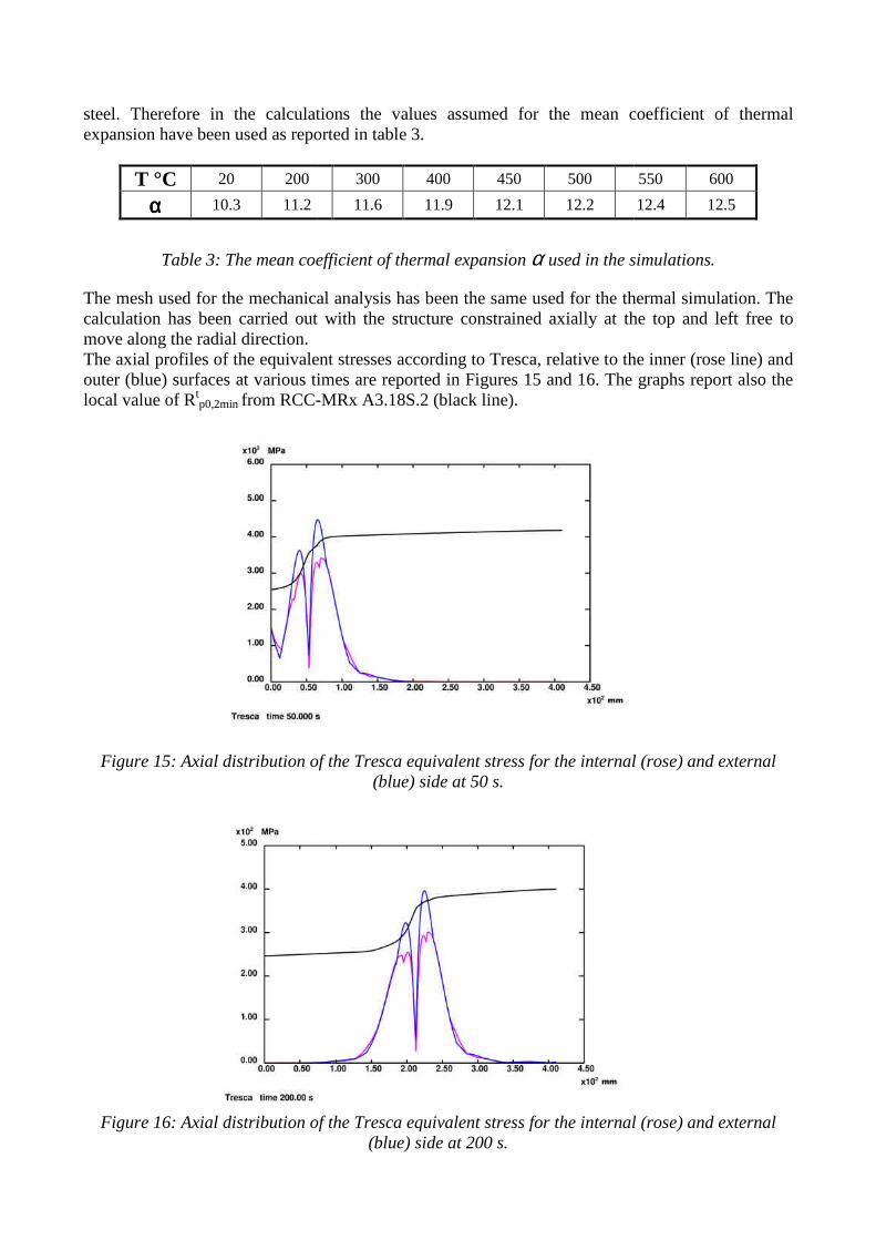
In the following figures (Figures and the experimentally detected profiles both for the temperature levels and for the dynamics of the front movement.

Figure 14 a): Comparison of the experimental and numerical axial temperature distribution at s, the green line indicates the position of the liquid surface

Figure 14 b): Comparison of the experimental and numerical axial temperature distribution at s, the green line indicates the position of the liquid surface

4.2 Mechanical analysis The mechanical calculation has been performed using CAST3M mechanical module [13]. The analysis was conducted in linear elasticity, consistently with the requirements of rules in RB 3231. The Young's modulus and the Poisson's ratio used in the calculations have been taken from RCC-MRx A3.18S.2. Regarding the thermal expansion coefficient, it has been found that the values reported in the standards are lower tha

Figures 14 a) and b)) we note the good agreement between the calculated and the experimentally detected profiles both for the temperature levels and for the dynamics of the

Comparison of the experimental and numerical axial temperature distribution at

the green line indicates the position of the liquid surface

Comparison of the experimental and numerical axial temperature distribution at

green line indicates the position of the liquid surface

The mechanical calculation has been performed using CAST3M mechanical module [13]. The analysis was conducted in linear elasticity, consistently with the requirements of

in RB 3231. The Young's modulus and the Poisson's ratio used in the calculations have been MRx A3.18S.2. Regarding the thermal expansion coefficient, it has been found

that the values reported in the standards are lower than those available in the literature for the P91

) we note the good agreement between the calculated and the experimentally detected profiles both for the temperature levels and for the dynamics of the

Comparison of the experimental and numerical axial temperature distribution at 100 the green line indicates the position of the liquid surface.

Comparison of the experimental and numerical axial temperature distribution at 200 green line indicates the position of the liquid surface.

The mechanical calculation has been performed using CAST3M mechanical module [13]. The analysis was conducted in linear elasticity, consistently with the requirements of the RCC-MRx

in RB 3231. The Young's modulus and the Poisson's ratio used in the calculations have been MRx A3.18S.2. Regarding the thermal expansion coefficient, it has been found

n those available in the literature for the P91

steel. Therefore in the calculations expansion have been used as reported in table

T °C 20 200

αααα 10.3 11.2

Table 3: The mean coefficient of thermal expansion

The mesh used for the mechanical analysis has been the same used for the thermal calculation has been carried out with the structure constrained move along the radial direction. The axial profiles of the equivalent stresses according to Tresca, relative to the inner (rose line) and outer (blue) surfaces at various times are reported in local value of Rtp0,2min from RCC-

Figure 15: Axial distribution of the Tresca equivalent stress for the internal (rose) and external

Figure 16: Axial distribution of the Tresca

steel. Therefore in the calculations the values assumed for the mean coefficient of thermal reported in table 3.

300 400 450 500

11.6 11.9 12.1 12.2

The mean coefficient of thermal expansion α used in the simulations

The mesh used for the mechanical analysis has been the same used for the thermal calculation has been carried out with the structure constrained axially at the top and left free to

The axial profiles of the equivalent stresses according to Tresca, relative to the inner (rose line) and ) surfaces at various times are reported in Figures 15 and 16. The grap

-MRx A3.18S.2 (black line).

Axial distribution of the Tresca equivalent stress for the internal (rose) and external

(blue) side at 50 s.

Axial distribution of the Tresca equivalent stress for the internal (rose) and external (blue) side at 200 s.

for the mean coefficient of thermal

550 600

12.4 12.5

used in the simulations.

The mesh used for the mechanical analysis has been the same used for the thermal simulation. The axially at the top and left free to

The axial profiles of the equivalent stresses according to Tresca, relative to the inner (rose line) and . The graphs report also the

Axial distribution of the Tresca equivalent stress for the internal (rose) and external

equivalent stress for the internal (rose) and external

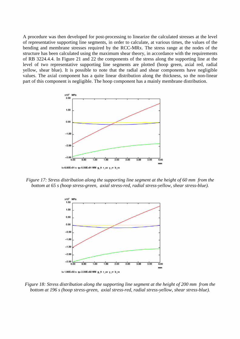
A procedure was then developedof representative supporting line segments, in order to calculate, at varioubending and membrane stresses required by the RCCstructure has been calculated using the maximum shear theory, in accordance with the requirements of RB 3224.4.4. In Figure 21 and level of two representative supporting line segmentsyellow, shear blue). It is possible to note that the radial and shear components have negligible values. The axial component has a quite linear distribution along the thickness, so the part of this component is negligible. The hoop component has a mainly membrane distribution.

Figure 17: Stress distribution along the supporting line segmebottom at 65 s (hoop stress-green,

Figure 18: Stress distribution along the supporting line segment at the height of bottom at 196 s (hoop stress-green,

A procedure was then developed for post-processing to linearize the calculated stresses at the level of representative supporting line segments, in order to calculate, at various times, the values of the bending and membrane stresses required by the RCC-MRx. The stress range at the nodes of the structure has been calculated using the maximum shear theory, in accordance with the requirements

and 22 the components of the stress along the supporting line level of two representative supporting line segments are plotted (hoop green, axial red, radial yellow, shear blue). It is possible to note that the radial and shear components have negligible alues. The axial component has a quite linear distribution along the thickness, so the

part of this component is negligible. The hoop component has a mainly membrane distribution.

Stress distribution along the supporting line segment at the height of 60 mm from the

green, axial stress-red, radial stress-yellow, shear stress

Stress distribution along the supporting line segment at the height of

green, axial stress-red, radial stress-yellow, shear stress

to linearize the calculated stresses at the level s times, the values of the

MRx. The stress range at the nodes of the structure has been calculated using the maximum shear theory, in accordance with the requirements

the components of the stress along the supporting line at the are plotted (hoop green, axial red, radial

yellow, shear blue). It is possible to note that the radial and shear components have negligible alues. The axial component has a quite linear distribution along the thickness, so the non-linear

part of this component is negligible. The hoop component has a mainly membrane distribution.

nt at the height of 60 mm from the yellow, shear stress-blue).

Stress distribution along the supporting line segment at the height of 200 mm from the yellow, shear stress-blue).

5. Verification of the conservatism of RCC-MRx RB 3261.1.1 for P91 The verification of the conservativism of the ratcheting rule RB 3261.1.1 in RCC-MRx for P91 steel requires a series of data obtained from both numerical calculations and experiments:

• The secondary stresses range ∆Q • The equivalent secondary membrane stress Qm • The maximum equivalent membrane stress Max(σm) • The temperature corresponding to maximum Qm

5.1 Determination of ∆Q The stress range ∆Q is calculated by linearizing the stresses originated from the secondary load, along the supporting line segment, according to RB 3224.5.5 and 3224.4.4, and considering the maximum value of the difference of the secondary membrane stress: ∆� = ��� ��� − �′�� (2) where t and tˈ are the times that maximize ∆Q. Table 4 reports the maximum values per cycle for the selected sections. 5.2 Determination of Qm Table 4 reports the two values of the equivalent secondary membrane stress Qm, corresponding to the passage of the cold side and hot side of the traveling temperature distribution. The first column in the table reports the distance of the section from the bottom of the sample. The average temperature on the section and the corresponding time are also reported.

5.3 Determination of secondary ratio SR and the efficiency index V The secondary ratio (RB 3261.1.1.1) has been calculated as follows SR= ∆Q/ Max(σm) (3)

Where Max (σm) is half the maximum of the membrane stress σm in correspondence of the hot side. In our case the primary loads are null and σm coincides with Qm. Moreover, since Qm is less than the yield stress, there is no need to apply the Neuber method. Since the secondary ratio SR results greater than 4, the efficiency index V is calculated with the RCC-MRx diagram as follows: V=1/SR0,5 (4) 5.4 Determination of the experimental efficiency index � The experimental efficiency index � is calculated as follows: � = Max(σm)/Peff_ex (5)

where Max(σm) is defined in (3) Peff_ex is calculated on the basis of the total deformations measured eP , according to A3.18AS.451 as follows: Peff_ex=C0 * (R

tp0,2 Exp) * (ep)

n0 (6)

Where C0 and n0 are the parameters given in table A3.18AS.451, Rt

p0,2 Exp is taken from Table 2 and ep is the experimental plastic strain. As stated in paragraph 3.2.2, the comparison between the efficiency index V and the experimental efficiency index � is carried out for two values of plastic strain:

• the plastic strain ep obtained considering the profile of the as received sample as baseline with a value of 0.22%,

• the plastic strain ep obtained considering the total deformation respect to the 8th cycle as baseline with a value of 0.10%.

The corresponding values of Peff_ex(0.10%), Peff_ex(0.22%), as well as the values of the experimental efficiency index � (0.10%) and � (0.22%) are reported in Table 4 for all the sections considered. 6. Discussion As show in Table 4 for all the sections considered and for both values of plastic strain considered, the efficiency index V, calculated according to RB3261.1113, results always higher than the experimental efficiency index �: � = ���σ��

����> � = ���σ��

����_�� (7)

Thus, it follows that P��� < P���_�� , that is: the effective primary stress evaluated according to the rule is lower than the value calculated on basis of the actual deformations. In other terms, the cumulated deformation predicted by the efficiency diagram is lower than the experimental one. These results confirm those obtained in P. Matheron et al. [6] by means of tension-torsion ratcheting tests performed on P91 tubular specimens. This is shown in Figure 19, where the experimental points have been represented in the space of the efficiency diagram variables (SR,�). It can be seen that all points representative of the tests are located under the efficiency diagram of RCC-MRx. Therefore, this diagram, in its present form, does not form a lower envelope for tests done with 9Cr steel. Its use for the design would foresee cumulative strains lower than those observed experimentally and is not conservative.

Figure 19 : Representation of the tests on the efficiency diagram.

The experimental results obtained in the framework of the MATTER project show therefore that the present efficiency diagram in RCC-MRx is not suited for 9Cr steels, both in the case of

“mechanical” and "thermal” ratcheting. Starting from these results, a new efficiency diagram could be defined as a lower envelope of the experimental points. It must be noted however that, in the efficiency diagram rule, the limitation of the ratcheting consists in defining an allowable value for the effective primary stress Peff. This value corresponds to a maximum allowable cumulative strain: in other words, the efficiency diagram rule allows to express a limit on the allowable strain as a limit on the allowable stress that can be calculated starting from the results of elastic analysis. The adaptation of the efficiency diagram rule to 9Cr steels implies therefore not only the development of a new efficiency diagram but also the definition of appropriate limits for Peff suited to P91. Considering the difference in behaviour between 9Cr steels and austenitic steels (strain hardening, cyclic hardening or softening), it is necessary to reconsider the stress limitation as a function of strain limits required for the material. In particular, it should be compatible with minimum values of total elongation under maximum load, which are much lower than those of austenitic steels. Particular attention should therefore be given to the limit of Peff in the case of 9Cr steel: this is however outside the scope of this work, whose aim was to verify the validity of the present efficiency diagram for 9Cr steels under thermal ratcheting. 7. Conclusions Modified 9Cr 1Mo steel, considered as structural material in several proposed Gen IV reactor concepts for out-of-core and for in-core components, due to its high yield strength, low thermal expansion coefficient and high thermal conductivity is extremely resistant to the thermal loads and thermal fatigue. On the other hand, because of its softening behaviour under cyclic loads, P91 is known to exhibits “material ratcheting” i.e. accumulation of plastic deformation. In the RCC-MRx code, the design assessment against ratcheting is performed by applying a simplified method, the efficiency diagram rule, based on elastic analysis of the structure. The efficiency diagram has been however been constructed and validated starting from a considerable number of results of experimental tests performed on austenitic stainless steels. It must therefore be reconsidered for 9Cr steels. Thermal ratcheting tests have been performed on a P91 mock-up in order to verify the applicability of the present RCC_MRX efficiency diagram rule for ratchetting to P91 Components. It has been considered the ratchetting induced by a moving axisymmetric temperature gradient with no primary loads applied. The thermal loads have been produced via hot liquid thermal shocks, by dipping a cylindrical mock-up in a molten eutectic mixture of sodium and potassium nitrides. The sample has been instrumented with thermocouples to follow the temperature evolution along the axis during the successive immersions. Measurements of the residual deformation were performed at selected cycles and show that the radius of the mock up shrank progressively in the region interested by the thermal loads. Finite element simulations where then performed to reconstruct the temperature profiles and stresses acting on the mock-up in order to obtain relevant quantities for the calculation of the efficiency index V as defined by the current diagram in the code. The comparison of the values where than compared with the values of the efficiency index experimentally determined which were found to be lower. Therefore, this diagram, in its present form, does not form a lower envelope for tests done with 9Cr steel and its application is not conservative. Its use for the design would predict to cumulative strains lower than those observed experimentally. This result confirms those obtained in previous tension-torsion ratcheting tests. The work performed in the framework of the MATTER project has paved the way for the development of a new efficiency diagram rule suited for 9Cr steels. This implies not only the development of a new efficiency diagram, but also the definition of appropriate stress limitations for the effective primary stress Peff. This limit must be defined as a function of the maximum allowable strain limits for this material, in particular the total strain under maximum load.

Acknowledgment The authors wish to acknowledge the support from the MATTER project under the umbrella of EERA Joint Program for Nuclear Materials (Grant Agreement n° 269706 – FP7-Fission-2010). References

1. K.L. Murty, I. Charit Journal of Nuclear Materials 383 (2008) 189–195 2. R. L. Klueh “Elevated temperature ferritic and martensitic steels and their application to

future nuclear reactors” ORNL/TM-2004/176 November 2004 3. L. Kunz , P. Luka´s Materials Science and Engineering A 319–321 (2001) 555–558 4. Koo, Gyeong-Hoi, Lee, Jae-Han International Journal of Pressure Vessels and Piping 84(5)

(2007) 284-292 5. H. Hübel Nuclear Engeneering and Design 162 (1996) 55–65 6. P. Matheron, G. Aiello, C. Caes, P. Lamagnere, A. Martin, M. Sauzay, Tension–torsion

ratcheting tests on 9Cr steel at high temperature, Nuclear Engineering and Design, 284 2015 207-214 ISSN 0029-5493,

7. T. Igari H. Wada M.Ueta Transactions of the ASME 122 (2000) 130-138 8. D.Watanabe, Y. Chuman, T. Otani, H. Shibamoto K. Inoue, N. Kasahara Nuclear

Engineering and Design 238 (2008) 389-398 9. H-Y Lee, J-B Kim and J-H Lee International Journal of Pressure Vessels and Piping 80

(2003) 41-48 10. ASME Section III Rules for construction of nuclear power plant components

Div. I-Subsection NH elevated temperature service 1998 edition 11. RCC-MRx "Règles de Conception et de construction des matériels Mécaniques des

installations nucléaires" (Design and construction rules for Mechanical equipment in nuclear facilities), AFCEN, 2013 edition

12. M.T. Cabrillat, J.M. Gatt, Y. Lejeail, A New Approach for Primary Overloads Allowance in Ratchetting Evaluation, Paper E4-456, SMIRT-13 E09-1 Porto Alegre Brazil 1995

13. Y Yang, M.T. Cabrillat SMIRT-18 F02-6 Beijing China 2005 14. S. Timoshenko , S. Woinowsky-Krieger, Theory of plates and shells, Mcgraw-Hill College,

2 edition June 1959 p. 480 15. CAST3M http://www-cast3m.cea.fr/

Table 4: Synoptic table for the verification of the conservatism of RCC-MRXRB 3261.1.1 for P91.

Sec.Lev

mm

ΔQ

MPa

Qm

MPa

Max(σm)

MPa

θm

°C

t

s

SR

-

V

-

Peff_ex(0,10%)

MPa

v(0,10%)

-

Peff_ex(0,22%)

MPa

v(0,22%)

-

36 849 240 102 25,5

“ 248 124 455 42 6,847 0,382 418 0,297 441 0,281

40 845 239 102 29

“ 246 123 457 46 6,870 0,382 417 0,295 440 0,280

60 812 251 116 48

“ 229 115 458 65 7,06 0,376 417 0,276 440 0,261

80 800 254 125 67

“ 222 111 458 84 7,207 0,372 417 0,276 440 0,252

100 785 249 133 86

217 109 459 103 7,202 0,373 417 0,261 439 0,248

150 751 238 142 133

208 104 455 150 7,221 0,372 418 0,249 441 0,236

200 724 230 148 180

200 100 441 196 7,24 0,372 422 0,236 445 0,225

250 702 222 143 226

195 98 445 244 7,16 0,374 421 0,233 444 0,221

300 401 199 126 270