117
Anomalous transport in a toroidal plasma Master Thesis Anne Schad Bergsaker December 2012
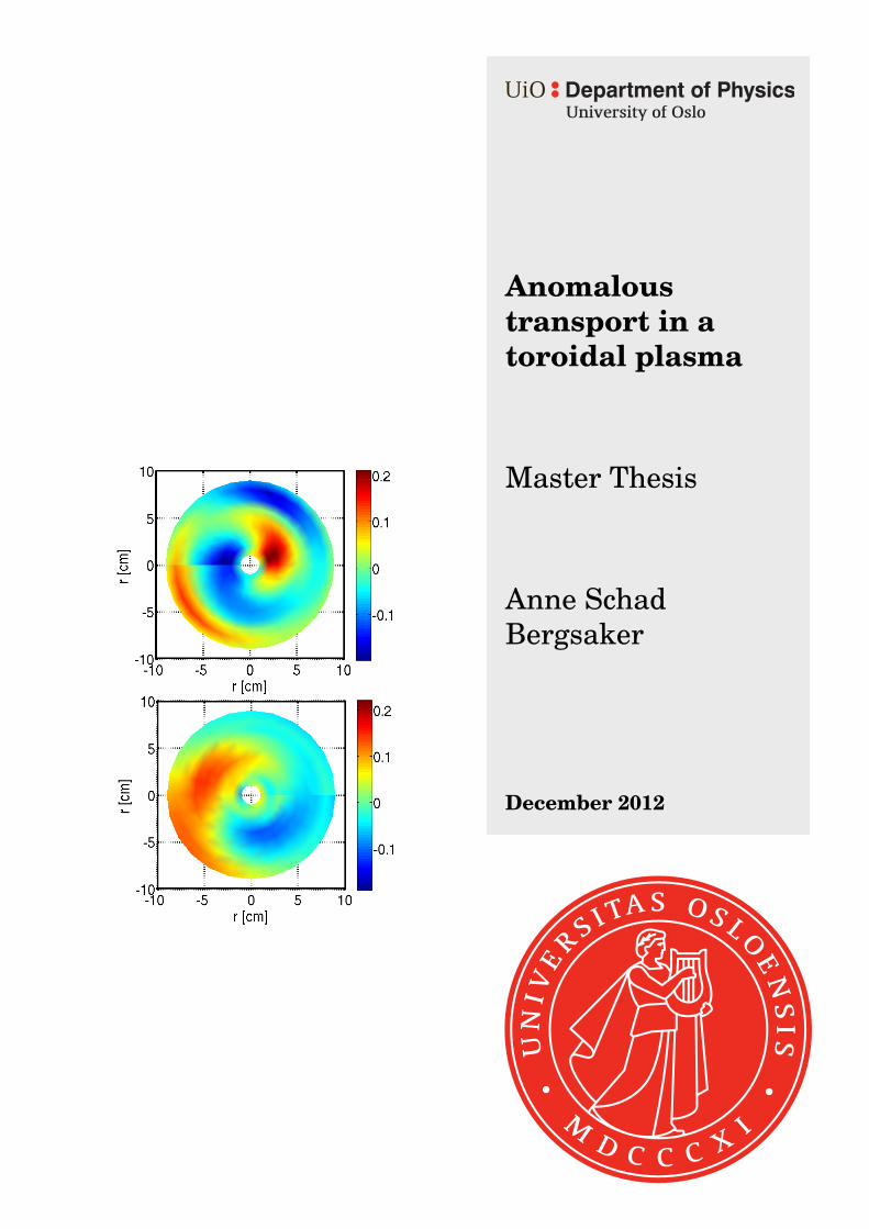
Anomaloustransport in atoroidal plasma
Master Thesis
Anne SchadBergsaker
December 2012

Abstract
Experimentally obtained data from the toroidal Blaamann device have been anal-ysed. Blaamann is a simple magnetised torus with no rotational transform, andplasma is generated by a discharge from a hot filament emitting electrons. The datawere obtained using a three pin Langmuir probe in combination with a stationaryreference probe. Sampled floating potential and electron saturation currents from19 different positions along the horizontal central line in a poloidal cross section,enabled us to study the turbulent transport within the plasma column.
Several statistical properties of the data were investigated. The average trans-port of flux is outwards, with large fluctuations in signals near the filament, butdecreasing with distance from the source. A clear and systematic relation betweenskewness and kurtosis was also identified.
Through use of cross correlation functions and the conditional sampling tech-nique we were able to investigate the nature of the anomalous transport, as wellas identify coherent structures. These structures appear to be burst-like in nature,with a lifetime of ∼ 100 µs. There is some indication that these structures arevortex-like. The coherent structures propagate around the poloidal cross sectionalong with the rest of the plasma column, rotating with the E × B/B2-velocity,and at the same time transporting plasma radially out of the column, giving riseto spiral trajectories.

ii Abstract

Acknowledgments
Firstly I would like to thank my supervisor Prof. Hans L. Pecseli for giving methis opportunity, and for all his help and advise throughout this process, and forreading through my thesis more times than I care to count. Your encouragementand guiding has been invaluable, and really I appreciate it.
I would also like to thank Prof. Ashild Fredriksen at the University of Tromsøfor all her help during my stay in Tromsø, and after. Thank you for not onlyputting up with all my e-mails, but actually answering them as well.
Prof. em. Jan Trulsen for taking an interest in my thesis, and offering insightfulcomments on my results.
Thanks to Hans Brenna, Christoffer Stausland, Elling Hauge-Iversen and allthe rest of you guys at the Plasma and space physics group for interesting andhelpful discussions, for happy lunch hours and good company.
And to AJ for reminding me that even physicists need some time off every nowand then.
Finally, the Magnifica, for making great coffee and keeping me awake and alertin these final stages.

iv Acknowledgments
Contents
Abstract i
Acknowledgments iii
1 Introduction 1
1.1 Motivation for this study . . . . . . . . . . . . . . . . . . . . . . . . 3
1.2 Structure of the thesis . . . . . . . . . . . . . . . . . . . . . . . . . 4
2 The basics of plasma physics 5
2.1 Basic plasma parameters . . . . . . . . . . . . . . . . . . . . . . . . 5
2.1.1 Thermal velocity . . . . . . . . . . . . . . . . . . . . . . . . 6
2.1.2 The plasma frequency . . . . . . . . . . . . . . . . . . . . . 6
2.1.3 The Debye length . . . . . . . . . . . . . . . . . . . . . . . . 6
2.1.4 The plasma parameter . . . . . . . . . . . . . . . . . . . . . 7
2.2 Single particle motion . . . . . . . . . . . . . . . . . . . . . . . . . 7
2.2.1 E×B-drift . . . . . . . . . . . . . . . . . . . . . . . . . . . 7
2.2.2 Curvature drift . . . . . . . . . . . . . . . . . . . . . . . . . 9
2.2.3 ∇B-drift . . . . . . . . . . . . . . . . . . . . . . . . . . . . . 10
2.2.4 Polarisation drift . . . . . . . . . . . . . . . . . . . . . . . . 10
2.3 Fluid model . . . . . . . . . . . . . . . . . . . . . . . . . . . . . . . 11
2.4 Plasma sheath and presheath . . . . . . . . . . . . . . . . . . . . . 11
2.4.1 Sheath region . . . . . . . . . . . . . . . . . . . . . . . . . . 12
2.4.2 The presheath . . . . . . . . . . . . . . . . . . . . . . . . . . 12
2.5 Langmuir probes . . . . . . . . . . . . . . . . . . . . . . . . . . . . 13
3 Turbulent plasma transport 15
3.1 Classical diffusion . . . . . . . . . . . . . . . . . . . . . . . . . . . . 15
3.2 Turbulent diffusion . . . . . . . . . . . . . . . . . . . . . . . . . . . 17
3.2.1 Single particle turbulent diffusion . . . . . . . . . . . . . . . 18
3.3 Plasma blob transport . . . . . . . . . . . . . . . . . . . . . . . . . 21
vi CONTENTS
4 The Blaamann experiment 254.1 The plasma tank . . . . . . . . . . . . . . . . . . . . . . . . . . . . 254.2 Probe diagnostics . . . . . . . . . . . . . . . . . . . . . . . . . . . . 264.3 Plasma rotation and drifts . . . . . . . . . . . . . . . . . . . . . . . 344.4 Fluctuating velocities . . . . . . . . . . . . . . . . . . . . . . . . . . 36
5 Methods 375.1 The probability density function . . . . . . . . . . . . . . . . . . . . 37
5.1.1 Theoretical model for the local particle flux . . . . . . . . . 385.2 Moments . . . . . . . . . . . . . . . . . . . . . . . . . . . . . . . . . 38
5.2.1 Skewness-kurtosis relations . . . . . . . . . . . . . . . . . . . 405.3 Correlation functions and power spectra . . . . . . . . . . . . . . . 435.4 Conditional sampling and averaging . . . . . . . . . . . . . . . . . . 45
5.4.1 Reference signals . . . . . . . . . . . . . . . . . . . . . . . . 47
6 Results 496.1 The raw data . . . . . . . . . . . . . . . . . . . . . . . . . . . . . . 496.2 PDFs . . . . . . . . . . . . . . . . . . . . . . . . . . . . . . . . . . . 51
6.2.1 Comparison with theoretical model for the flux distribution . 536.2.2 Joint PDF for velocity and density . . . . . . . . . . . . . . 53
6.3 Moments . . . . . . . . . . . . . . . . . . . . . . . . . . . . . . . . . 576.3.1 Skewness/kurtosis relation for plasma flux . . . . . . . . . . 596.3.2 Skewness/variance relation for plasma flux . . . . . . . . . . 60
6.4 Correlation functions . . . . . . . . . . . . . . . . . . . . . . . . . . 626.4.1 Autocorrelation functions and power spectra . . . . . . . . . 626.4.2 Cross correlation . . . . . . . . . . . . . . . . . . . . . . . . 62
6.5 Conditional sampling . . . . . . . . . . . . . . . . . . . . . . . . . . 676.5.1 Outward bursts . . . . . . . . . . . . . . . . . . . . . . . . . 676.5.2 Inward transport . . . . . . . . . . . . . . . . . . . . . . . . 756.5.3 Dynamics of the flux-component . . . . . . . . . . . . . . . . 776.5.4 Conditional variance . . . . . . . . . . . . . . . . . . . . . . 80
7 Discussion and conclusion 837.1 Statistical properties . . . . . . . . . . . . . . . . . . . . . . . . . . 83
7.1.1 General properties of the plasma fluctuations . . . . . . . . . 837.1.2 Skewness kurtosis relations . . . . . . . . . . . . . . . . . . . 84
7.2 Coherent structures . . . . . . . . . . . . . . . . . . . . . . . . . . . 857.3 Anomalous transport . . . . . . . . . . . . . . . . . . . . . . . . . . 86
7.3.1 Vortex structures . . . . . . . . . . . . . . . . . . . . . . . . 877.4 Summary . . . . . . . . . . . . . . . . . . . . . . . . . . . . . . . . 887.5 Future perspectives . . . . . . . . . . . . . . . . . . . . . . . . . . . 89
CONTENTS vii
A Source code 91A.1 Plotting samples of raw data . . . . . . . . . . . . . . . . . . . . . . 92A.2 Probability density functions . . . . . . . . . . . . . . . . . . . . . . 92
A.2.1 Experimental data . . . . . . . . . . . . . . . . . . . . . . . 92A.2.2 Theoretical model . . . . . . . . . . . . . . . . . . . . . . . . 93A.2.3 Joint PDF . . . . . . . . . . . . . . . . . . . . . . . . . . . . 94
A.3 Statisitical moments . . . . . . . . . . . . . . . . . . . . . . . . . . 95A.3.1 All sets treated as one long string of data . . . . . . . . . . . 95A.3.2 All sets treated separately . . . . . . . . . . . . . . . . . . . 97A.3.3 Including the Argon plasma data . . . . . . . . . . . . . . . 99
A.4 Autocorrelation and FFT . . . . . . . . . . . . . . . . . . . . . . . 100A.5 Cross correlation . . . . . . . . . . . . . . . . . . . . . . . . . . . . 101A.6 Conditional sampling . . . . . . . . . . . . . . . . . . . . . . . . . . 102
Bibliography 105

viii CONTENTS
Chapter 1
Introduction
Plasma is a partially or fully ionised gas in which a portion of the electrons and ionscan move about freely. The ionisation makes plasma significantly different fromclassical neutral gases since the charged components have a high mobility. Thisallows the flow of charged particles that generates currents and magnetic fields.Forces due to electromagnetic effects are important in describing the propertiesand dynamics of plasmas, as electric and magnetic forces allow the particles tointeract over large distances. Since plasma is in nature so different from a gas, itis often referred to as the fourth state of matter.
Even though over 90% of all visible matter in the universe consists of plasma,it was not discovered until the late 1800s, when Sir William Crookes conducted hisexperiments on Crookes tubes discovering what he referred to as radiant matter(Crookes, 1879). The term plasma was first used by Irving Langmuir in 1928(Langmuir, 1928). He needed to find a name for the non-sheath region of thedischarge in mercury, and he did not wish to invent a new word. Somehow hefound inspiration in the medical term blood plasma, even though his colleagueTonks later specified that Langmuir did not in any way see gaseous plasma as ananalogue to the liquid component of blood (Tonks, 1967).
Plasma is formed in the Earth’s near as well as more distant environment,i.e. in the ionosphere and magnetosphere as well as in distant space. Study andmodelling of plasmas is therefore to some extent motivated by the need to havespace equipment, such as satellites and rockets functioning in an environmentdominated by plasma. Industrial plasmas on the other hand are used for variousprocesses, perhaps the most notable of which is thermonuclear fusion, which is seenas a promising new way of generating electricity. Through thermonuclear fusion,the goal is to achieve a steady state referred to as self-sustained burn, which meansthat once the process is started it will continue in principle indefinitely, generatingenergy. Many different devices were considered originally, where early suggestionsconsisted of various pinch-types (Bishop, 1958). In modern days most devices have
2 Introduction
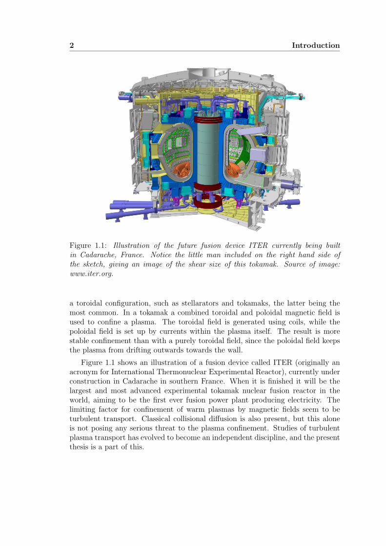
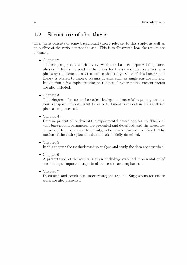
Figure 1.1: Illustration of the future fusion device ITER currently being builtin Cadarache, France. Notice the little man included on the right hand side ofthe sketch, giving an image of the shear size of this tokamak. Source of image:www.iter.org.
a toroidal configuration, such as stellarators and tokamaks, the latter being themost common. In a tokamak a combined toroidal and poloidal magnetic field isused to confine a plasma. The toroidal field is generated using coils, while thepoloidal field is set up by currents within the plasma itself. The result is morestable confinement than with a purely toroidal field, since the poloidal field keepsthe plasma from drifting outwards towards the wall.
Figure 1.1 shows an illustration of a fusion device called ITER (originally anacronym for International Thermonuclear Experimental Reactor), currently underconstruction in Cadarache in southern France. When it is finished it will be thelargest and most advanced experimental tokamak nuclear fusion reactor in theworld, aiming to be the first ever fusion power plant producing electricity. Thelimiting factor for confinement of warm plasmas by magnetic fields seem to beturbulent transport. Classical collisional diffusion is also present, but this aloneis not posing any serious threat to the plasma confinement. Studies of turbulentplasma transport has evolved to become an independent discipline, and the presentthesis is a part of this.
Motivation for this study 3
The experimental data analysed in this study are from an experiment con-ducted with the Blaamann plasma device. It is a simple magnetised torus, whichmeans it has a simple magnetic configuration. The magnetic field is purely toroidal,with no poloidal component, i.e. there is no rotational transform. The Blaamanndevice consists of a rather small toroidal tank. Originally it was constructed andset up in 1989 at the University in Tromsø, though it does not remain there today.Blaamann is not a fusion device, but a tank designed to do simple experimentson toroidal plasma. In the present study we intend to focus on anomalous, i.e.non-collisional transport within the plasma column, looking at both statisticalproperties of the fluctuating density, velocity and flux, as well as singling outlarger events. The latter is to enable us to to investigate the possibility that wehave larger coherent structures, and if so, how they are transported within theplasma. As there is no poloidal field to help with confinement, we have some lossof plasma as it is transported outwards, but this is on average balanced by theproduction of plasma over time (Rypdal et al., 1994).
1.1 Motivation for this study
The overall aim of this thesis is to study the anomalous transport within a toroidalplasma. Turbulent flows have a unique ability to disperse particles at a rate whichgreatly exceeds transport by classical molecular diffusion. The dominant mecha-nism within turbulent transport in plasmas is in many cases found to be transportdue to low-frequency electrostatic waves that are strongly magnetic field aligned.However, in this study we will focus on analysing the turbulent fluctuations, whilethe driving mechanism (a plasma instability) will not be addressed.
Turbulence in itself is difficult to simulate realistically, as most systems tend tobe too complex to cover all contributing factors. Experimental data offer a uniqueinsight into the turbulent nature of plasmas, without requiring great computationalresources beyond handling and treating the recorded data. Even though we onlyhave data along the horizontal midline of a circular cross section we intend toshow that much can still be deduced concerning transport within the entire crosssection, and consequently the entire plasma column.
In addition, simple magnetised tori play in important role in the understandingof tokamak transport. It is easier to accomplish a good comparison between theoryand experiment when dealing with a simpler case. Studying the results from adevice such as Blaamann offers a chance to check theoretical models against realexperimental results.
4 Introduction
1.2 Structure of the thesis
This thesis consists of some background theory relevant to this study, as well asan outline of the various methods used. This is to illustrated how the results areobtained.
Chapter 2This chapter presents a brief overview of some basic concepts within plasmaphysics. This is included in the thesis for the sake of completeness, em-phasising the elements most useful to this study. Some of this backgroundtheory is related to general plasma physics, such as single particle motion.In addition a few topics relating to the actual experimental measurementsare also included.
Chapter 3This chapter offers some theoretical background material regarding anoma-lous transport. Two different types of turbulent transport in a magnetisedplasma are presented.
Chapter 4Here we present an outline of the experimental device and set-up. The rele-vant background parameters are presented and described, and the necessaryconversion from raw data to density, velocity and flux are explained. Themotion of the entire plasma column is also briefly described.
Chapter 5In this chapter the methods used to analyse and study the data are described.
Chapter 6A presentation of the results is given, including graphical representation ofour findings. Important aspects of the results are emphasised.
Chapter 7Discussion and conclusion, interpreting the results. Suggestions for futurework are also presented.
Chapter 2
The basics of plasma physics
Since plasma differs significantly from all other states of matter, a brief overviewof the basic concepts regarding the general description of a plasma is included inthis chapter. The motion occurring within a plasma due to electric and magneticforces is also described here, as this is very relevant to the plasma motion withinBlaamann. As this is a study of experimental data, a short introduction to themechanics of basic probes is also included, as well as concepts that are relevantfor plasma confinement.
An important concept in plasma physics is quasi-neutrality. A plasma is said tobe quasi-neutral as long as the total number of electrons on a large scale is roughlythe same as the number of ions, i.e. overall the electric charge of the plasma isclose to zero. There can still occur small perturbations, but this happens only onsmall characteristic time and length-scales, and will generally be shielded by thesurrounding plasma.
When dealing with highly dilute plasmas, it is convenient to describe the motionin the plasma by single particle motion. In such cases no collective interactionneeds to be taken into account, and only the background fields affecting the chargedparticle is needed to describe the motion. However, if the density of the plasmais sufficiently large, interactions mediated by electric and magnetic forces has tobe accounted for. Interaction can be assumed to occur in essentially two differentways. One possibility is that we have collisional processes, i.e. interaction betweenonly two particles at a time. The other possibility is that we have a large numberof particles that simultaneously affect the motion of one selected reference particle.
2.1 Basic plasma parameters
There are four parameters that prove useful when describing a plasma. Theseare the thermal velocity, the plasma frequency, the Debye length and the plasma

6 The basics of plasma physics
parameter. Therefore brief definitions of all four are included here. In this studywe use the definition where the temperature is given in eV, which is equivalent toa temperature in Kelvin satisfying the relation κT = eφ.
2.1.1 Thermal velocity
The thermal velocity is the typical velocity of the thermal motion of the particlesin a fluid or gas. Hence it is also a measure of temperature. The definition usedhere is
uth,s =
(eTsms
)1/2
, (2.1)
where e is elementary charge, Ts is the temperature given in eV and ms themass of particle species s. This definition has excluded a numerical constant forsimplicity. The expression is found numerically from conservation of energy, i.e.from 1
2ms〈u2〉 = 3
2eTs for monoatomic gases with three degrees of freedom, and
u2th = 〈u2〉.
2.1.2 The plasma frequency
A characteristic time scale is the inverse of the plasma frequency, ωpe, defined as
ωpe =
(e2n
ε0me
)1/2
, (2.2)
where n is the number density and me is the electron mass. Consider a slab ofplasma within which the electrons have been slightly displaced with respect to theions. This small perturbation in the charge density distribution sets up an electricfield. Since the electrons are much smaller and lighter than the ions, they arealso much more mobile. The result is that the electrons start to oscillate aboutthe equilibrium position with a characteristic frequency ωpe. The correspondingplasma period is then τp = 2π/ωpe.
2.1.3 The Debye length
The characteristic length scale in a plasma is the Debye length, λDe.
λDe =
(ε0Teen
)1/2
(2.3)
A plasma particle moving with the thermal velocity uth will travel one Debyelength in one plasma period. Physically, this distance characterises a shielding
Single particle motion 7
distance. When a single charge q is introduced into a plasma, the surroundingparticles of opposite charge will attempt to screen off the electric potential arisingdue to q. The result is that further away from the charge, this minor perturbationis close to undetectable, and only the collective behaviour of all the particles inthe plasma can be observed. At a distance of one Debye length from q, the electricpotential of this charge is reduced by a factor of e−1, i.e. the charge is shielded bythe surrounding plasma.
2.1.4 The plasma parameter
From the Debye length and the plasma density the plasma parameter can beconstructed.
Np = nλ3De (2.4)
This dimensionless quantity is related to the average number of particles containedwithin a sphere with radius λDe. As long as the number of particles within theDebye sphere is large, any small perturbation within it will not be noticed a certaindistance from it. This is because the many other particles within the sphereshield off any small perturbation, thus the overall electric field is not noticeablyinfluenced. However, if the number of particles within the Debye sphere is low,any change of the charge distribution within it might have a significant effect onthe surroundings, and the electric field might be perturbed. Thus the plasmaparameter is a tool that enables us to predict whether a plasma will be dominatedby the discrete nature of the particles, or their collective behaviour. We have thatλ3De ∼ n−3/2T 1/2, which means that Np ∼ n−1/2T 3/2. This means that Np will
increase either if T increases or n decreases. Thus any plasma with Np 1 willbe hot and dilute.
2.2 Single particle motion
The simplest version of a plasma imaginable is a plasma consisting of only oneparticle. This may seem like a gross oversimplification, but it turns out that thebehaviour that can be deduced for a single particle in magnetic and electric fields,is also applicable to more complex plasmas.
2.2.1 E×B-drift
The most significant force affecting a particle travelling through a combined electricand magnetic field is the Lorentz force,
F = q(E + U×B) . (2.5)
8 The basics of plasma physics
Consider a particle with charge q and mass m moving with a velocity U througha uniform B-field. The equation of motion for the particle is then
md
dtU⊥ = qU⊥ ×B . (2.6)
The magnetic field cannot impart any energy to a charged particle, since the forceis perpendicular to the displacement. As the acceleration is perpendicular to U⊥,we have that U⊥ is constant in magnitude but not in direction. The result is thatthe particle will gyrate in a circular orbit with a radius given by the initial velocity,the Larmor radius
rL =mU⊥qB
, (2.7)
and a frequency known as the cyclotron frequency
Ωc =qB
m. (2.8)
If one should also introduce a constant electric field with a component perpen-dicular to the magnetic field, the resulting equation of motion would be
md
dtU = q(E⊥ + U×B) . (2.9)
By introducing a new velocity U∗ ≡ U − E⊥ × B/B2, where U is the originalvelocity, it can be shown that the resulting velocity consists of two parts. Oneaccounting for the gyromotion due to the magnetic field, and one accounting forthe average motion of the gyro-centre. The latter is given below and is generallyknown as the E×B-velocity.
UE×B =E⊥ ×B
B2(2.10)
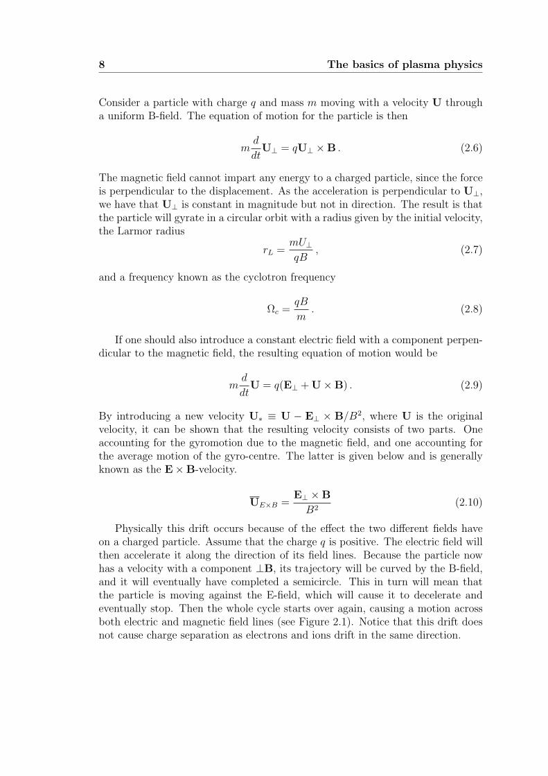
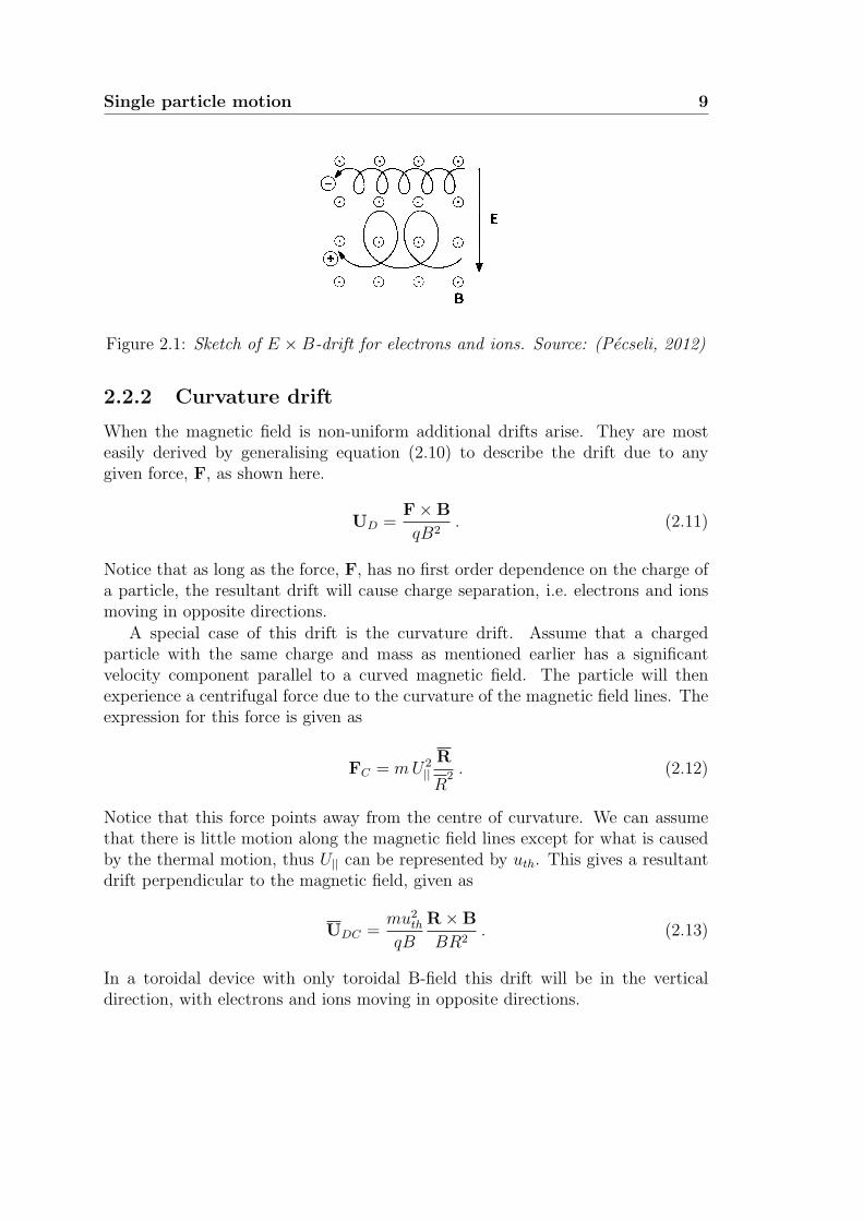
Physically this drift occurs because of the effect the two different fields haveon a charged particle. Assume that the charge q is positive. The electric field willthen accelerate it along the direction of its field lines. Because the particle nowhas a velocity with a component ⊥B, its trajectory will be curved by the B-field,and it will eventually have completed a semicircle. This in turn will mean thatthe particle is moving against the E-field, which will cause it to decelerate andeventually stop. Then the whole cycle starts over again, causing a motion acrossboth electric and magnetic field lines (see Figure 2.1). Notice that this drift doesnot cause charge separation as electrons and ions drift in the same direction.
Single particle motion 9
Figure 2.1: Sketch of E ×B-drift for electrons and ions. Source: (Pecseli, 2012)
2.2.2 Curvature drift
When the magnetic field is non-uniform additional drifts arise. They are mosteasily derived by generalising equation (2.10) to describe the drift due to anygiven force, F, as shown here.
UD =F×B
qB2. (2.11)
Notice that as long as the force, F, has no first order dependence on the charge ofa particle, the resultant drift will cause charge separation, i.e. electrons and ionsmoving in opposite directions.
A special case of this drift is the curvature drift. Assume that a chargedparticle with the same charge and mass as mentioned earlier has a significantvelocity component parallel to a curved magnetic field. The particle will thenexperience a centrifugal force due to the curvature of the magnetic field lines. Theexpression for this force is given as
FC = mU2||
R
R2 . (2.12)
Notice that this force points away from the centre of curvature. We can assumethat there is little motion along the magnetic field lines except for what is causedby the thermal motion, thus U|| can be represented by uth. This gives a resultantdrift perpendicular to the magnetic field, given as
UDC =mu2
th
qB
R×B
BR2. (2.13)
In a toroidal device with only toroidal B-field this drift will be in the verticaldirection, with electrons and ions moving in opposite directions.
10 The basics of plasma physics
∆
|B|
B
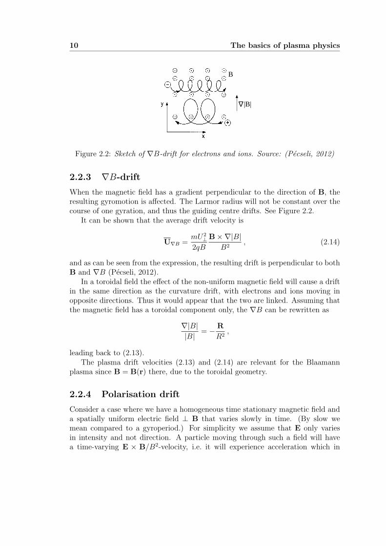
Figure 2.2: Sketch of ∇B-drift for electrons and ions. Source: (Pecseli, 2012)
2.2.3 ∇B-drift
When the magnetic field has a gradient perpendicular to the direction of B, theresulting gyromotion is affected. The Larmor radius will not be constant over thecourse of one gyration, and thus the guiding centre drifts. See Figure 2.2.
It can be shown that the average drift velocity is
U∇B =mU2
⊥2qB
B×∇|B|B2
, (2.14)
and as can be seen from the expression, the resulting drift is perpendicular to bothB and ∇B (Pecseli, 2012).
In a toroidal field the effect of the non-uniform magnetic field will cause a driftin the same direction as the curvature drift, with electrons and ions moving inopposite directions. Thus it would appear that the two are linked. Assuming thatthe magnetic field has a toroidal component only, the ∇B can be rewritten as
∇|B||B|
= − R
R2,
leading back to (2.13).The plasma drift velocities (2.13) and (2.14) are relevant for the Blaamann
plasma since B = B(r) there, due to the toroidal geometry.
2.2.4 Polarisation drift
Consider a case where we have a homogeneous time stationary magnetic field anda spatially uniform electric field ⊥ B that varies slowly in time. (By slow wemean compared to a gyroperiod.) For simplicity we assume that E only variesin intensity and not direction. A particle moving through such a field will havea time-varying E × B/B2-velocity, i.e. it will experience acceleration which in
Fluid model 11
the particles own frame of reference can be interpreted as a form of an artificialgravitational acceleration, g. This gravitational acceleration is given as the timederivative of the E×B/B2-velocity
g = −(
1
B2
)d
dt(E×B) .
The resulting force F = mg gives rise to the following velocity
Up =m
eB2
d
dtE . (2.15)
This drift velocity is called the polarisation drift and it is dependent on charge.Electrons and ions will move in opposite directions.
Equivalently, this can be used to describe the drift of a particle moving througha spatially inhomogeneous time-stationary electric field, since the particle willexperience this as d
dtE 6= 0 in its own frame of reference.
In Blaamann we have an electric field that consists of a time-stationary radialbackground field, E0, with an additional fluctuating component, causing an E ×B/B2 as well as a polarisation drift.
2.3 Fluid model
When treating a plasma consisting of many particles, it is possible to treat thisas an N -body problem, taking into account all the forces acting on every singleparticle, including interaction effects. However, when investigating macroscopicprocesses, it is much simpler to treat a plasma as a conducting fluid, and it turnsout that the two different models yield the same results as long as the analysis iscarried out consistently to the same order (Goldston and Rutherford, 1995).
The fluid model treats the plasma as a collection of fluid elements, thus onlyevaluating bulk parameters. These include particle density, flow velocity, currentdensity, charge density and temperature over a collection of particles within a fluidelement. Since this study is based on experimental data containing measurementsof bulk parameters, and the spatial resolution is such that any microscopic effectswould not be detected, it will be reasonable to treat the plasma tube containedwithin the Blaamann plasma tank as an electromagnetic fluid.
2.4 Plasma sheath and presheath
Any quasi-neutral plasma contained in a vacuum chamber will be joined to surfacesby a thin positively charged layer called a sheath. These arguments will in principlealso apply to probe surfaces and similar.
12 The basics of plasma physics
2.4.1 Sheath region
Assume we have a plasma contained within a vacuum chamber, and that there isonly a negligible electric field present. This means that the potential within theplasma is ∼ 0. When electrons and ions collide with the wall they recombine, andare thus lost. As electrons are significantly more mobile than ions, they are lostmore quickly, resulting in a build-up of positive charge near the wall. Thereforea potential must exist to contain the more mobile charged species, allowing theflow of positive and negative particles to the wall to be balanced (Chen, 1984).The non-neutral potential region between the quasi-neutral plasma and the wallis called a sheath, and is typically a few λDe wide. An ion entering the sheath willthen be accelerated towards the wall, while an electron will be reflected back intothe plasma. The electron density near the wall will always be less than the iondensity, as it decays on the order of a Debye length, shielding the electrons fromthe wall.
The Bohm sheath criterion states that the velocity of an ion in the sheath mustbe greater than or equal to the Bohm velocity, uB
us ≥ uB =
(eTeM
)1/2
, (2.16)
where Te is given in electronvolts. The Bohm velocity is in itself the acousticvelocity of ions, and thus ions are supersonic in the sheath. (Chen, 1984; Liebermanand Lichtenberg, 2005)
2.4.2 The presheath
In order to ensure continuity of ion flux, there must be a finite electric field in theplasma over the same area, generally much wider than the sheath. This region iscalled the presheath. The presheath itself is not field free, but E is very small here,so there is a small potential drop. This potential drop accelerates the ions to theBohm velocity, causing a transition from subsonic flow velocity in the bulk plasmato supersonic flow in the sheath. At the exact boundary between the sheath andthe presheath, the ions have a velocity equal to the Bohm velocity.
In Blaamann we will have sheaths and presheaths both surrounding the outerwall, but also around the Langmuir probes used to measure floating potentialand electron saturation current. The nature of the sheath and presheath regionsmust be taken into account when using the data to find the corresponding densityfluctuations.
Langmuir probes 13
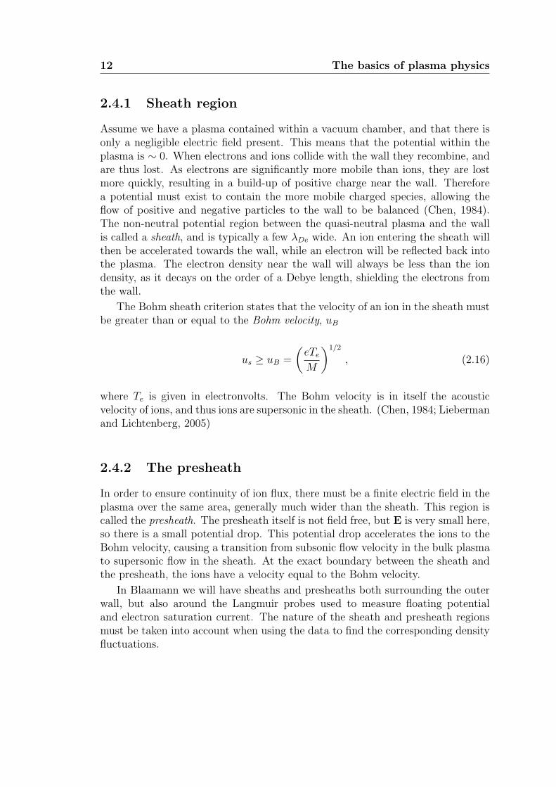
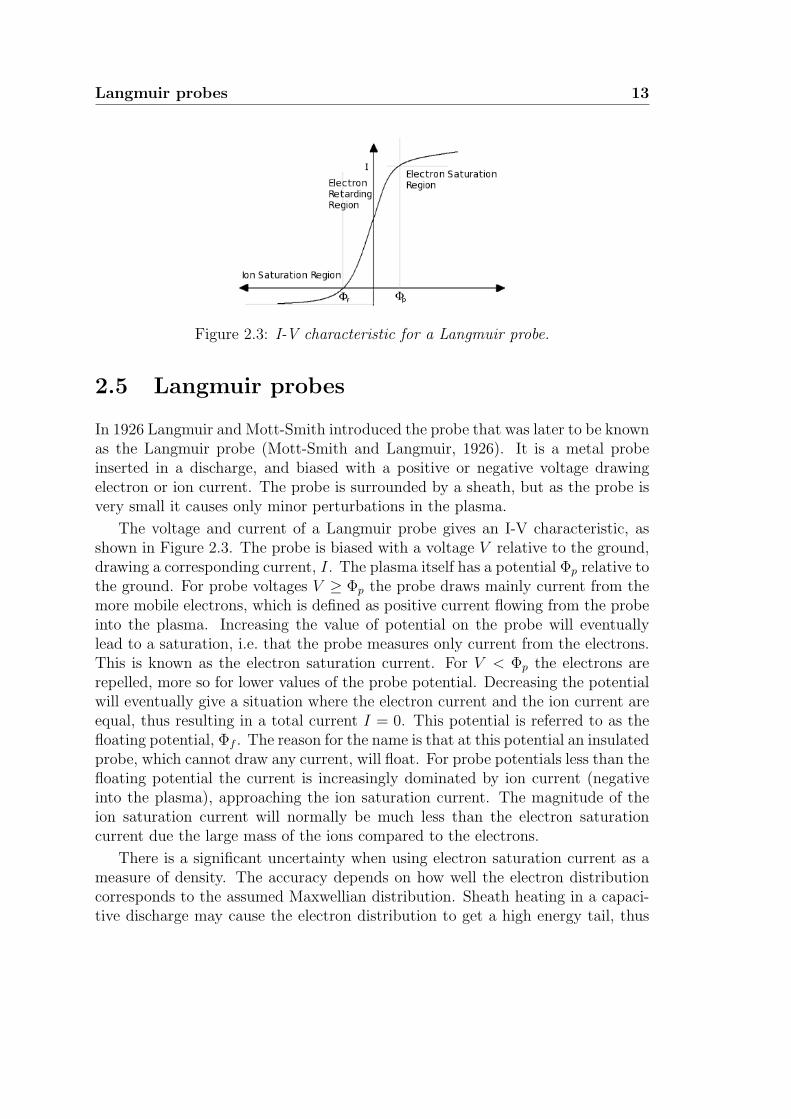
Figure 2.3: I-V characteristic for a Langmuir probe.
2.5 Langmuir probes
In 1926 Langmuir and Mott-Smith introduced the probe that was later to be knownas the Langmuir probe (Mott-Smith and Langmuir, 1926). It is a metal probeinserted in a discharge, and biased with a positive or negative voltage drawingelectron or ion current. The probe is surrounded by a sheath, but as the probe isvery small it causes only minor perturbations in the plasma.
The voltage and current of a Langmuir probe gives an I-V characteristic, asshown in Figure 2.3. The probe is biased with a voltage V relative to the ground,drawing a corresponding current, I. The plasma itself has a potential Φp relative tothe ground. For probe voltages V ≥ Φp the probe draws mainly current from themore mobile electrons, which is defined as positive current flowing from the probeinto the plasma. Increasing the value of potential on the probe will eventuallylead to a saturation, i.e. that the probe measures only current from the electrons.This is known as the electron saturation current. For V < Φp the electrons arerepelled, more so for lower values of the probe potential. Decreasing the potentialwill eventually give a situation where the electron current and the ion current areequal, thus resulting in a total current I = 0. This potential is referred to as thefloating potential, Φf . The reason for the name is that at this potential an insulatedprobe, which cannot draw any current, will float. For probe potentials less than thefloating potential the current is increasingly dominated by ion current (negativeinto the plasma), approaching the ion saturation current. The magnitude of theion saturation current will normally be much less than the electron saturationcurrent due the large mass of the ions compared to the electrons.
There is a significant uncertainty when using electron saturation current as ameasure of density. The accuracy depends on how well the electron distributioncorresponds to the assumed Maxwellian distribution. Sheath heating in a capaci-tive discharge may cause the electron distribution to get a high energy tail, thus
14 The basics of plasma physics
leaving the bulk electrons significantly colder than assumed through equilibriumdischarge with a Maxwellian distribution (Lieberman and Lichtenberg, 2005).
In this study cylindrical probes were used to measure floating potential andelectron saturation current. However, electron diffusion across magnetic field linesis greatly inhibited.
D⊥ =D||
1 + ω2cτ
2c
,
where ωc is the gyration frequency, τc is the mean collision time, and D|| is thedrift coefficient along B while D⊥ is the drift coefficient ⊥ B. Because of this acylindrical probe drawing electron current will behave similarly to a plane probemeasuring conditions where there is no magnetic field. The only difference is thatthe effective probe area becomes equal to the probe cross section along the fieldlines, rather than the actual surface area of the cylindrical probe. Since the probeonly collects electrons from a thin plasma layer corresponding to two times theprobe cross section (front and back), it can be treated like a plane probe.
Chapter 3
Turbulent plasma transport
It has been shown by Rypdal et al. (1994) that no classical mechanisms can accountfor the transport of charge from the filament to the wall in Blaamann. Bothexperimental and theoretical evidence suggests that the charge transport is dueto turbulent processes, and that this turbulence is also what causes the cross fieldplasma transport. However, the question is whether this turbulence in mainlydiffusive or burst-like is nature.
This chapter outlines the mechanisms of turbulent diffusion as well as plasmablob transport.
3.1 Classical diffusion
In classical diffusion collisions between particles cause them to wander significantdistances from their respective starting positions. In a non-uniform plasma theresult of such motion is a net migration of particles from an area with high densityto one with lower density, thus levelling out any large scale density gradients.Mathematically it is described by the diffusion equation in one spatial dimension
∂n
∂t=
∂
∂x
(D∂n
∂x
), (3.1)
where D is the diffusion coefficient.A simple and illustrative way of describing diffusion is the random walk model.
Assuming a number of particles are moving randomly along a straight line with astep length of ∆x taken at equal intervals of time ∆t, we can estimate the averagemotion. If there are many similar particles that all start out from x = 0, all withan equal chance of moving to the left or to the right, the average position of thegroup of particles will be
〈x〉 = 0
16 Turbulent plasma transport
at any given time. However, after some time the group will have spread out. Eventhough it will have spread a nearly equal distance on either side, the root-mean-square position will not be zero. It can be shown that this quantity increases intime as
d
dt〈x2〉 =
(∆x)2
∆t,
which gives
〈x2〉 =(∆x)2t
∆t,
where the aforementioned diffusion coefficient is related through D ∼ (∆x)2/∆t.Thus in classical diffusion the spread of the particles goes as 〈x2〉 ∼ t.
This can be generalised to three dimensions, with the diffusion equation be-coming
∂n
∂t= ∇ · (D∇n) . (3.2)
Note that since charged particles can move freely along magnetic field lines, dif-fusion parallel to the magnetic field is reduced by collisions. However, diffusionacross the magnetic field is enhanced by collisions. We will focus on transportacross B.
As D has dimension [D] = length2/time, it seems reasonable that we canestimate the diffusion coefficient for diffusion due to electron-ion collisions by atypical step length and the time between collisions. The latter is merely theinverse of the collision frequency, νie. A typical step length will be given by theLarmor radius, but it is important to keep in mind that rL is much greater forions than for electrons. In a magnetic field conservation of momentum demandsthat the gyro-centre of two particles with equal but opposite charge must movethe same distance after a collision, because we must have q1∆r
(1)c + q2∆r
(2)c = 0.
rc is the position of the respective gyro-centres. This means that even though anion in principle could move a typical step length ∼ rLi, it is bound by the electronLarmor radius. Thus both electrons and ions will have a typical step length of∼ rLe (Pecseli, 2012).
For a fully ionised plasma we have D⊥ ∼ r2Leνei. Inserting (2.7) for rLe and
νei ∼ ωpe/Np, we find that
D⊥ ∼n
B2√T.
This means that increasing the magnetic field strength will reduce collisional dif-fusion, as will increasing the temperature or reducing the density. Physically wehave that when the magnetic field strength is increased, the Larmor radius de-creases. This means that both electrons and ions gyrate in smaller circles, and thedistance travelled due to a collisions is smaller. Thus more collisions are needed
Turbulent diffusion 17
for a charged particle to be able to escape the bulk plasma. Similarly, if the tem-perature is increased we get an increase in Np, giving a corresponding decreasein collision frequency. If there are less collisions, the motion of charged particlesacross magnetic field lines will be slower. Increasing the particle density will nat-urally give a greater collisions frequency, as there will be more particles to collidewith. Consequently we will have an increase in collisional diffusion across B.
The scaling remains accurate (with a different numerical factor) for collisionswith neutrals. Ions will then not be bound by the electron Larmor radius, but theelectron and ion dynamics are locked by the requirement of quasi-neutrality, andas an order of magnitude the coefficient retains the electron Larmor radius as aneffective length scale, with appropriate collision frequency.
3.2 Turbulent diffusion
One of the most important properties of turbulent flows is their ability to disperseparticles at a rate which by far exceeds transport by classical molecular diffusion.This is a property of both neutral fluids and plasmas alike. Whenever there is adensity gradient in a plasma, a drift wave instability will eventually occur, settingup a transverse isobar wavefront in the plasma between dense and less dense areas.During the linear growth phase, the drift wave instability is closely connected withparticle transport along the direction of the density gradient. The question ishow the saturated turbulent fluctuating field (assuming that such a state exists)transports particles.
First we make some general remarks on this problem, and present some ofthe basic results on turbulent diffusion. The outline is independent of the dimen-sionality of the problem and the ideas apply equally well for three dimensionaland two dimensional turbulence, assuming the plasma to be homogeneous andisotropic. Particle displacement will be expressed in terms of a velocity, but thisvelocity can be obtained from an electrostatic electric field in magnetized plasmasas u(r, t) = E(r, t) × B0/B0 for homogeneous magnetic fields. We assume lowfrequency turbulence in which relevant frequencies are ω Ωci, where Ωci is theion cyclotron frequency. This model will then assume two dimensional turbulencein the plane ⊥ B0. Polarisation drifts along ∂E/∂t are ignored, i.e. to the accuracy〈ω〉/Ωci ≈ 10−3.
Many experiments have demonstrated that turbulent transport is an impor-tant mechanism in for instance fusion plasma experiments (Liewer, 1985), andsignificant efforts have been made to understand this mechanism for anomaloustransport also in the context of drift wave turbulence (Horton, 1999).

18 Turbulent plasma transport
3.2.1 Single particle turbulent diffusion
We start by considering the simplest possible problem, namely the one where asingle particle is released in a homogeneous and isotropic turbulent velocity field,u(r, t). Assuming that the particle is convected passively by the flow, we want todetermine its mean square displacement with respect to the origin of release. Forsimplicity we take this to be at the origin (Roberts, 1957).
Since, by assumption, dr(t)/dt = u(r(t), t), we have in a given realisation ofthe flow that the particle position is given as
r(t) =
∫ t
0
u(r(t′), t′)dt′ . (3.3)
The average position 〈r(t)〉 vanishes, since we have assumed 〈u(r(t), t)〉 = 0. Thisis actually not quite as self evident as it might appear, since we can assume fromthe outset only that 〈u(r, t)〉 = 0, but this is concerning a function of a spatial aswell as a temporal variable, while 〈u(r(t), t)〉 is a function of time alone.
The mean square displacement is a positive quantity, and we find
r(t) · dr(t)
dt=
1
2
dr2(t)
dt= u(r(t), t) ·
∫ t
0
u(r(t′), t′)dt′ =
∫ t
0
u(r(t), t) · u(r(t′), t′)dt′ .
(3.4)Taking the ensemble average, we have
d
dt
⟨r2(t)
⟩= 2
∫ t
0
〈u(r(t), t) · u(r(t′), t′)〉 dt′ . (3.5)
For time stationary turbulence we have a dependence of time separations only suchas
〈u(r(t), t) · u(r(t′), t′)〉 = RL(t− t′)〈u2〉
with the subscript L reminding us to sample the velocity field along a Lagrangianorbit, i.e. follows the path of the single particle. We introduced RL as the nor-malised Lagrangian velocity correlation function, RL(0) = 1. By the assumptionof time stationary Lagrangian velocities, we implicitly assume that all spatial po-sitions visited by the randomly moving particle are statistically similar, i.e. weassume the turbulent velocity field to be spatially homogeneous.
When integrating (3.4) as
⟨r2(t)
⟩= 2〈u2〉
∫ t
0
∫ t′′
0
RL(t′′ − t′)dt′dt′′
Turbulent diffusion 19
it is an advantage to introduce the variables τ ≡ t′′ − t′ and s ≡ t′′, giving theJacobian
J =
∂τ
∂t′′∂τ
∂t′
∂s
∂t′′∂s
∂t′
=1 -11 0
= 1
so that dt′′dt′ = dτds. Transforming the variables as indicated, we note that wecan change the order of integration as∫ t
0
∫ s
0
RL(τ)dτds =
∫ t
0
∫ t
τ
RL(τ)dsdτ
=
∫ t
0
RL(τ)
∫ t
τ
dsdτ
=
∫ t
0
RL(τ)(t− τ)dτ
to give ⟨r2(t)
⟩= 2t〈u2〉
∫ t
0
(1− τ/t)RL(τ)dτ . (3.6)
Two relevant limiting cases of (3.6) can be distinguished here (Roberts, 1957).
1. Very short times, where it can be assumed that the correlation functionRL(τ) ≈ 1. In this limit we find⟨
r2(t)⟩≈ 〈u2〉t2
which is often called the ballistic limit since it is the result we would haveobtained by assuming the particle to follow straight lines of orbit, r(t) = ut,and simply average over all velocities. This kind of motion will be burst-like.One can experience finding auto-correlation functions that are not differen-tiable for τ = 0, and in such cases the ballistic limit does not exist. Suchcases require that 〈(du/dt)2〉 diverges. With finite particle inertia we wouldexpect that du/dt should be finite at all times. The absence of a ballisticlimit simply indicates a very rapidly changing velocity field, and the intervalwhere RL(τ) ≈ 1 may be negligible.
2. Very large times, t → ∞, where it can be assumed that∫ t
0RL(τ)dτ ≈ τL,
introducing the Lagrangian integral correlation time
τL ≡∫ ∞
0
RL(τ)dτ . (3.7)
20 Turbulent plasma transport
In this limit we find the important result⟨r2(t)
⟩≈ 2tτL〈u2〉 . (3.8)
At least formally this looks like the result one obtains by using the classicaldiffusion equation with a diffusion coefficient D ≡ 2τL〈u2〉 to obtain themean square particle displacement. Such cases have⟨
r2(t)⟩∼ t .
The limit of times much larger than the Lagrangian correlation time is con-sequently called the diffusion limit. This limiting case is consistent with arandom walk with a typical length step τL
√〈u2〉 per time τL, consistent with
a mixing length model.
By the assumption of a stationary random process for the turbulent velocityfield, i.e. averages depend on time differences only and not absolute times,we are in effect implying that the process is also spatially homogeneous.Otherwise the particle would occupy, from time to time during its randommotion, spatial regimes where the statistical properties of u(r, t) differedfrom the rest of the flow. Was this the case, we would experience sequencesof the Lagrangian temporal velocity signal, where the statistical propertieswere distinguishable from the rest.
In reality we will never experience a fully homogeneous random vector field.However, for some finite time interval where a particle is, by high proba-bility, confined to a locally homogeneous field we might use such idealisedapproximations. In the Blaamann plasma we might assume local spatial ho-mogeneity in a “doughnut-shaped” region around the origin (x, y) = (0, 0)(see Figure 4.5). Within this region it might be possible to observe the dif-fusion limit, in principle. We will find, however, that no such diffusion limitwill be identified with the analysis tools used in this project.
Note that r(t) is not a time-stationary random process, although it is derivedfrom u(r, t) which can be assumed to be so. The initial time (the time when theparticle was released) has a special role for r(t).
Introducing the Lagrangian power spectrum,
SL(ω) ≡ (1/2π)
∫ ∞−∞
RL(t)e−iωtdt ,
with
RL(t) =
∫ ∞−∞
SL(ω)eiωtdω ,
Plasma blob transport 21
we can write the result (3.6) on the form
⟨r2(t)
⟩= t2 〈u2〉
∫ ∞−∞
(sin(ωt/2)
ωt/2
)2
SL(ω)dτ . (3.9)
The function sin2(ωt/2)/(ωt/2)2 originates from the Fourier transform of the “tri-angular” function 1 − τ/t entering the convolution (3.6). For large times it isevident that dispersion of the test particle is primarily due to the low frequenciesin the Lagrangian spectrum. We have
limt→∞
sinωt/2
ω/2= πδ(ω) ,
so we recover τL = SL(ω = 0). Note that oscillations in the Lagrangian spectrumwith frequencies being multiples of 1/t do not contribute to the particle displace-ment. This is because they return the particle to its starting point after a time t.Often it is assumed that low frequencies in (3.9) corresponds to large wavelengths(or rather large scales), but we should be aware that there is no a priori reason toexpect this.
By (3.9) our problem seems to be solved once and for all, at least for the caseof homogeneous isotropic turbulence. However, it is not so, since we do not knowthe spectrum SL(ω), and it is very complicated to obtain it experimentally. Ithas been a major enterprise over the years to find ways of predicting SL(ω) onthe basis of the more readily measurable Eulerian correlation function. Amazinglygood results can be obtained, at least as far as predictions of 〈r2(t)〉 are concerned.However, this might as well imply that this is a very robust result, and that almostany reasonable guess on RL will give acceptable results. After all, we must requirethat RL(0) = 1 and that RL(t → ∞) → 0, and with a little common sense allreasonable guesses of RL tend to look more or less the same.
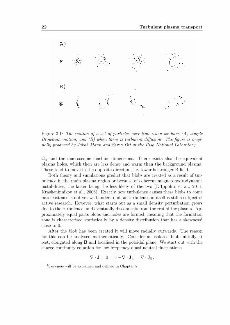
The asymptotic stage of turbulent transport is diffusion-like but the interme-diate steps are very different as illustrated in Figure 3.1.
3.3 Plasma blob transport
An alternative method of transport within plasma across magnetic field lines isblob transport. A blob is a plasma structure that is elongated along the magneticfield. It is significantly denser and warmer than the surrounding plasma, and highlylimited in size across magnetic field lines. It travels in the radial direction fromstrong magnetic fields to weaker, i.e. in the direction of −∇B. In a torus this wouldmean motion towards the outer wall on the low field side. They are also referred toas mesoscale structures because their perpendicular size is intermediate between
22 Turbulent plasma transport
Figure 3.1: The motion of a set of particles over time when we have (A) simpleBrownian motion, and (B) when there is turbulent diffusion. The figure is origi-nally produced by Jakob Mann and Søren Ott at the Risø National Laboratory.
Ωci and the macroscopic machine dimensions. There exists also the equivalentplasma holes, which then are less dense and warm than the background plasma.These tend to move in the opposite direction, i.e. towards stronger B-field.
Both theory and simulations predict that blobs are created as a result of tur-bulence in the main plasma region or because of coherent magnetohydrodynamicinstabilities, the latter being the less likely of the two (D’Ippolito et al., 2011;Krasheninnikov et al., 2008). Exactly how turbulence causes these blobs to comeinto existence is not yet well understood, as turbulence in itself is still a subject ofactive research. However, what starts out as a small density perturbation growsdue to the turbulence, and eventually disconnects from the rest of the plasma. Ap-proximately equal parts blobs and holes are formed, meaning that the formationzone is characterised statistically by a density distribution that has a skewness1
close to 0.After the blob has been created it will move radially outwards. The reason
for this can be analysed mathematically. Consider an isolated blob initially atrest, elongated along B and localised in the poloidal plane. We start out with thecharge continuity equation for low frequency quasi-neutral fluctuations
∇ · J = 0 =⇒ −∇ · J⊥ = ∇ · J|| ,1Skewness will be explained and defined in Chapter 5
Plasma blob transport 23
where J⊥ is the perpendicular current density and J|| is the magnetic field-alignedcurrent density. The perpendicular current can be written as a sum of the plasmainertia current and the current due to guiding centre drifts. If the magnetic field isnon-uniform, we will have guiding centre drifts due to ∇B and curvature, causinga current
JB =P
Bb× (κ+∇ lnB) , (3.10)
where b is a unit vector in the direction of B, P is the plasma pressure andκ = (b ·∇)b the magnetic field curvature vector. As κ is pointing inwards towardsthe centre of the torus and the magnetic field oriented along the toroidal direction(counter clockwise when viewed from above), the current density JB sets up anelectric field within the blob, pointing downwards. The resultant E×B-drift willthen be radially outwards towards the outer edge of the torus.
Inserting (3.10) into the continuity equation gives
∇ ·(ρmB
d
dt
∇⊥φB
)+
1
Bb× (κ+∇ lnB) · ∇P = ∇ · J||
where the first term is the plasma inertia current (Garcia, 2009). ρm is the plasmamass density and φ the electrostatic potential. The left hand side of this equationgives a relationship between speed of the blob Cb and parameters such as sizeacross field lines, `, pressure amplitude within the blob, ∆P , and curvature radiusof the magnetic field, R.
CbCs∼(
2`
R
∆P
Π
)1/2
.
Π is the background plasma pressure. This shows that a larger or denser blobwill move faster than a smaller, more dilute blob. Numerical simulations of blobstructures with a Gaussian pressure distribution have shown that a blob startingout from rest will have a radial drift at the centre of the structure, but as theblob accelerates, the structure itself changes shape, and an asymmetric wavefrontforms with a steep front and a trailing wake, giving it a characteristic mushroom-like shape. In some cases the blob will distort further, and eventually dissolvecompletely.
The experimental definition of a blob has varied in literature, depending onthe data available. Generally, the very minimum required for a positive identifi-cation of a blob is a single point measurement of a density distribution which ispositively skewed and non-Gaussian in the outer midplane, as this is indicative ofa large positive density perturbation passing the probe. However, distinguishingbetween a non-Gaussian blob-like structure and the Gaussian background tendsto be difficult, since the blob itself has developed from this Gaussian backgroundturbulence.

24 Turbulent plasma transport
In the presence of blobs in toroidal plasma, the skewness of the density distri-bution tends to increase with increased distance from the blob birth zone. In somecases the skewness will be negative closer to the plasma centre, indicating plasmaholes having propagated inwards. Near the birth zone the blobs tend to be smalland hard to detect, but closer to the outer wall, blobs are expected to be largeand dominant. Because of the asymmetry due to magnetic curvature in a toroidaldevice giving a toroidal field, it is somewhat unclear whether blobs exist in theinside regions of the torus, and also in which direction they might propagate.
Blobs contribute large positive burst in the density time signal. Probe measure-ments of identifiable blobs have shown that the probability distribution of particledensity signals are positively skewed and have heavy tails due to the many largebursts in the time series, hence also the kurtosis is expected to be greater than 3,which is the kurtosis of a random Gaussian process. However, though a densitydistribution with positive skewness and large kurtosis are characteristic when wehave blob transport, they are not necessarily evidence of the presence of blobs inthe plasma.
Chapter 4
The Blaamann experiment
4.1 The plasma tank
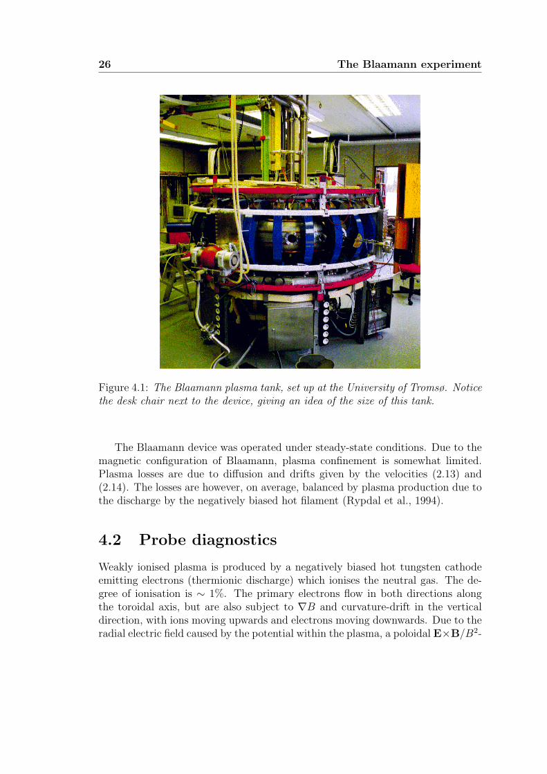
In 1989 the Blaamann plasma experiment (see Figure 4.1) was constructed at theUniversity of Tromsø. The purpose of the device was to offer the opportunity tostudy the behaviour of turbulent weakly magnetised plasma, as well as instabil-ities and anomalous transport. This was done by confining plasma on magneticfield lines within a toroidal vacuum chamber and measuring spatial and temporalchanges in density, potential difference and electron temperature across a poloidalcross section. A thorough description of both how Blaamann was built and howit works in detail can be found in Rypdal et al. (1994) and Brundtland (1992).Here we will give a brief description in order to illustrate how the experiment inquestion was conducted, and how the data were obtained.
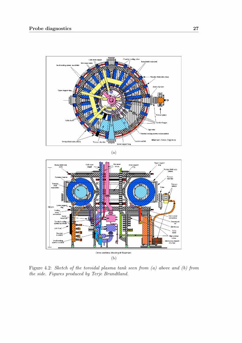
Schematic set-up of the experiment is shown in Figure 4.2a) (from above) andb) (from the side). The experiment consists of a stainless steel vacuum chambershaped like a torus with major radius R = 651.5 mm and minor radius r = 133.5mm, hence the width of the chamber is small compared to the major circumference.The chamber itself is comprised of four 90 degree bends connected together withconflat flanges, and each section has a sector chamber for improved access. 24circular coils (marked blue) provide a toroidal magnetic field of up to 0.4 T. Thisfield is almost homogeneous with a magnetic ripple δB/B that varies from 0.002in the central part of the poloidal cross section to 0.01 near the outer wall. Eighthorizontally positioned coils centred around the major axis can provide small radialand vertical magnetic fields (marked red and white respectively). All along thesurface of the tank is a series of square copper tubes working as water cooling. Inaddition there is also a vacuum pump and a power supply. The entire set-up isheld in place by a supporting rack as indicated by the dark grey sections in Figure4.2. The entire device weighs about 350 kg.
26 The Blaamann experiment
Figure 4.1: The Blaamann plasma tank, set up at the University of Tromsø. Noticethe desk chair next to the device, giving an idea of the size of this tank.
The Blaamann device was operated under steady-state conditions. Due to themagnetic configuration of Blaamann, plasma confinement is somewhat limited.Plasma losses are due to diffusion and drifts given by the velocities (2.13) and(2.14). The losses are however, on average, balanced by plasma production due tothe discharge by the negatively biased hot filament (Rypdal et al., 1994).
4.2 Probe diagnostics
Weakly ionised plasma is produced by a negatively biased hot tungsten cathodeemitting electrons (thermionic discharge) which ionises the neutral gas. The de-gree of ionisation is ∼ 1%. The primary electrons flow in both directions alongthe toroidal axis, but are also subject to ∇B and curvature-drift in the verticaldirection, with ions moving upwards and electrons moving downwards. Due to theradial electric field caused by the potential within the plasma, a poloidal E×B/B2-
Probe diagnostics 27
(a)
(b)
Figure 4.2: Sketch of the toroidal plasma tank seen from (a) above and (b) fromthe side. Figures produced by Terje Brundtland.
28 The Blaamann experiment
drift is also set up, causing a rotation of the plasma column. A circular poloidallimiter extending 2.5 cm inwards from the wall receives any discharge current be-tween the filament and the ground. Since there is no toroidal electric current norpoloidal magnetic field except the radial and vertical fields which can be imposed,there is no rotational transform. A steady state situation is achieved where theplasma generation and losses are balanced. Note that this condition should herebe understood to mean in an averaged sense.
The experiment in question was carried out in August 2003. It was conductedusing helium plasma held at a constant background pressure of ∼ 2.0 × 10⁻⁴
mbar and with a discharge current of 1.0 A. The toroidal field current was 350A, resulting in a magnetic field strength of 1540 G (0.154 T) at a reference pointin the centre of a poloidal cross section. The filament was biased at 140 V withrespect to the surrounding walls. The electric field E and the plasma density nhave both a dc and a fluctuating component, while the magnetic field is consideredto be constant in time. We assume quasi-neutrality, i.e. n = ne ≈ ni.
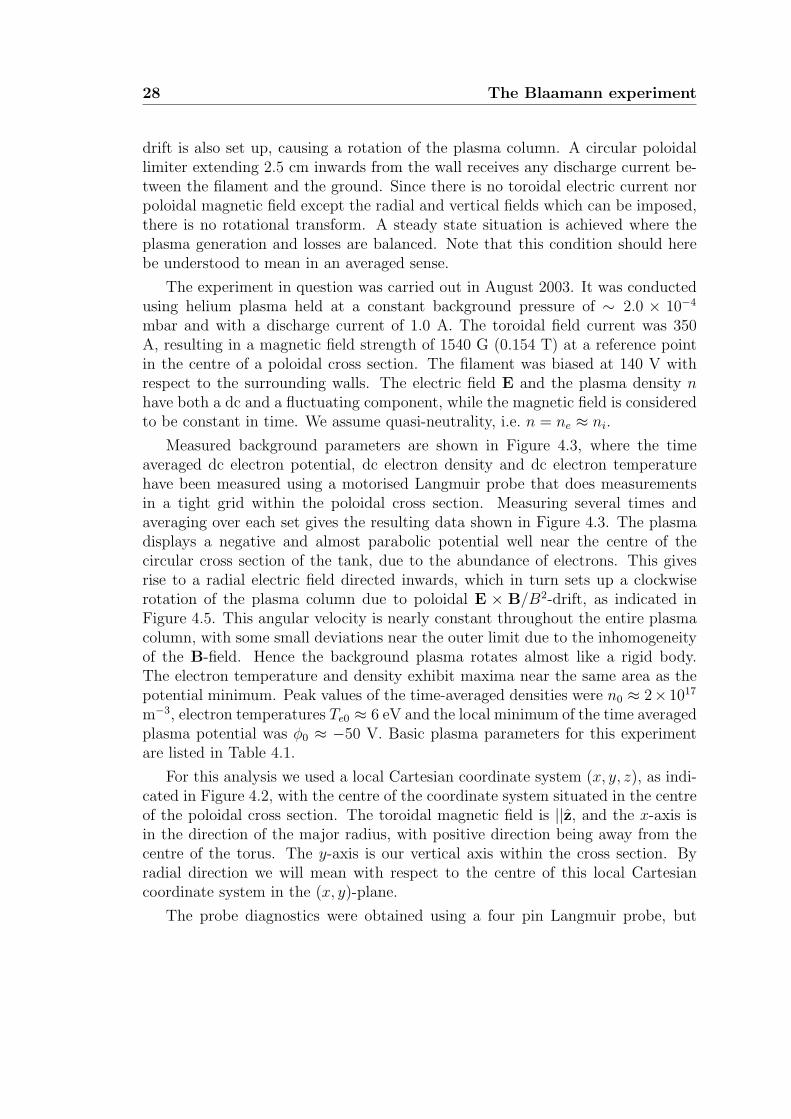
Measured background parameters are shown in Figure 4.3, where the timeaveraged dc electron potential, dc electron density and dc electron temperaturehave been measured using a motorised Langmuir probe that does measurementsin a tight grid within the poloidal cross section. Measuring several times andaveraging over each set gives the resulting data shown in Figure 4.3. The plasmadisplays a negative and almost parabolic potential well near the centre of thecircular cross section of the tank, due to the abundance of electrons. This givesrise to a radial electric field directed inwards, which in turn sets up a clockwiserotation of the plasma column due to poloidal E × B/B2-drift, as indicated inFigure 4.5. This angular velocity is nearly constant throughout the entire plasmacolumn, with some small deviations near the outer limit due to the inhomogeneityof the B-field. Hence the background plasma rotates almost like a rigid body.The electron temperature and density exhibit maxima near the same area as thepotential minimum. Peak values of the time-averaged densities were n0 ≈ 2× 10¹⁷
m−3, electron temperatures Te0 ≈ 6 eV and the local minimum of the time averagedplasma potential was φ0 ≈ −50 V. Basic plasma parameters for this experimentare listed in Table 4.1.
For this analysis we used a local Cartesian coordinate system (x, y, z), as indi-cated in Figure 4.2, with the centre of the coordinate system situated in the centreof the poloidal cross section. The toroidal magnetic field is ||z, and the x-axis isin the direction of the major radius, with positive direction being away from thecentre of the torus. The y-axis is our vertical axis within the cross section. Byradial direction we will mean with respect to the centre of this local Cartesiancoordinate system in the (x, y)-plane.
The probe diagnostics were obtained using a four pin Langmuir probe, but
Probe diagnostics 29
Figure 4.3: The dc electron density Ne, dc electron temperature Te and dc plasmapotential Vp for a poloidal cross section. All parameters are time averaged andobtained using a computer controlled motorised Langmuir probe. The coordinate(0, 0) is taken to be the middle of a poloidal cross section. The vertical filamentis placed near where Ne has a sharp maximum, and Te displays an elongated peak.Figure provided by Ashild Fredriksen.
only three of the pins were actually in use. In addition to this there was also afixed reference probe. All probes were 5 mm long and had a radius of 0.125 mm.The constellation is shown in Figure 4.5. The reference probe was positioned at5 cm above the horizontal centre line of the poloidal cross section indicated bya small circle in the figure, and measured floating potential. The four pin probewas movable along the horizontal midplane and consisted of two pins measuringpotential and one measuring electron saturation current, with the fourth pin beingobsolete. Measurements were done along the horizontal centre line in positionsfrom x = −9 cm to x = +9 cm, in leaps of one cm, giving a total of 19 differentpositions. At every position 5 datasets were collected. The data was digitizedusing a 12-bit digitizer at a sampling rate of 250 kHz with 104 samples per set,
30 The Blaamann experiment
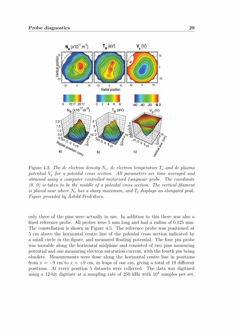
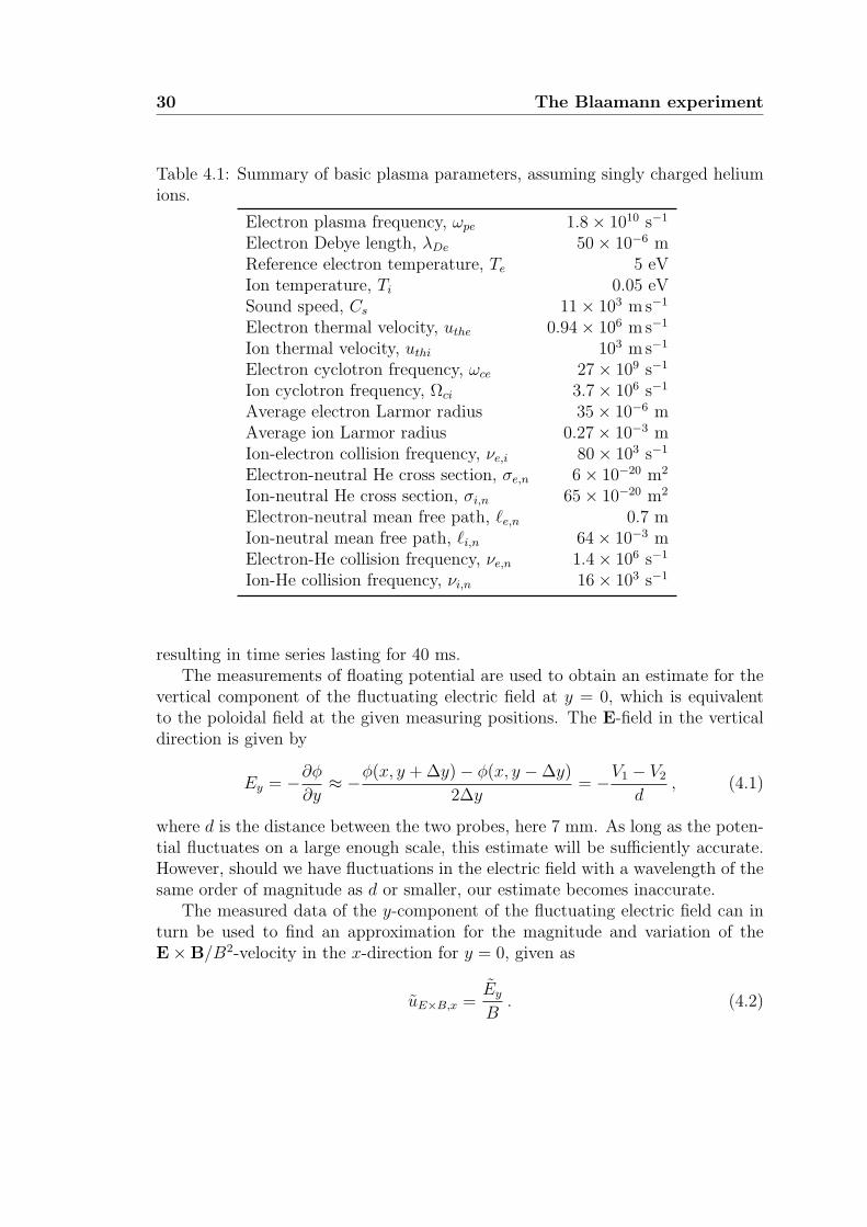
Table 4.1: Summary of basic plasma parameters, assuming singly charged heliumions.
Electron plasma frequency, ωpe 1.8× 10¹⁰ s−1
Electron Debye length, λDe 50× 10−6 mReference electron temperature, Te 5 eVIon temperature, Ti 0.05 eVSound speed, Cs 11× 103 m s−1
Electron thermal velocity, uthe 0.94× 10⁶ m s−1
Ion thermal velocity, uthi 103 m s−1
Electron cyclotron frequency, ωce 27× 109 s−1
Ion cyclotron frequency, Ωci 3.7× 10⁶ s−1
Average electron Larmor radius 35× 10−6 mAverage ion Larmor radius 0.27× 10⁻³ mIon-electron collision frequency, νe,i 80× 103 s−1
Electron-neutral He cross section, σe,n 6× 10⁻²⁰ m2
Ion-neutral He cross section, σi,n 65× 10−20 m2
Electron-neutral mean free path, `e,n 0.7 mIon-neutral mean free path, `i,n 64× 10−3 mElectron-He collision frequency, νe,n 1.4× 10⁶ s−1
Ion-He collision frequency, νi,n 16× 103 s−1
resulting in time series lasting for 40 ms.The measurements of floating potential are used to obtain an estimate for the
vertical component of the fluctuating electric field at y = 0, which is equivalentto the poloidal field at the given measuring positions. The E-field in the verticaldirection is given by
Ey = −∂φ∂y≈ −φ(x, y + ∆y)− φ(x, y −∆y)
2∆y= −V1 − V2
d, (4.1)
where d is the distance between the two probes, here 7 mm. As long as the poten-tial fluctuates on a large enough scale, this estimate will be sufficiently accurate.However, should we have fluctuations in the electric field with a wavelength of thesame order of magnitude as d or smaller, our estimate becomes inaccurate.
The measured data of the y-component of the fluctuating electric field can inturn be used to find an approximation for the magnitude and variation of theE×B/B2-velocity in the x-direction for y = 0, given as
uE×B,x =EyB. (4.2)
Probe diagnostics 31
−60 −40 −20 0 20 40 600
50−10
0
10
R0
r0
x
y
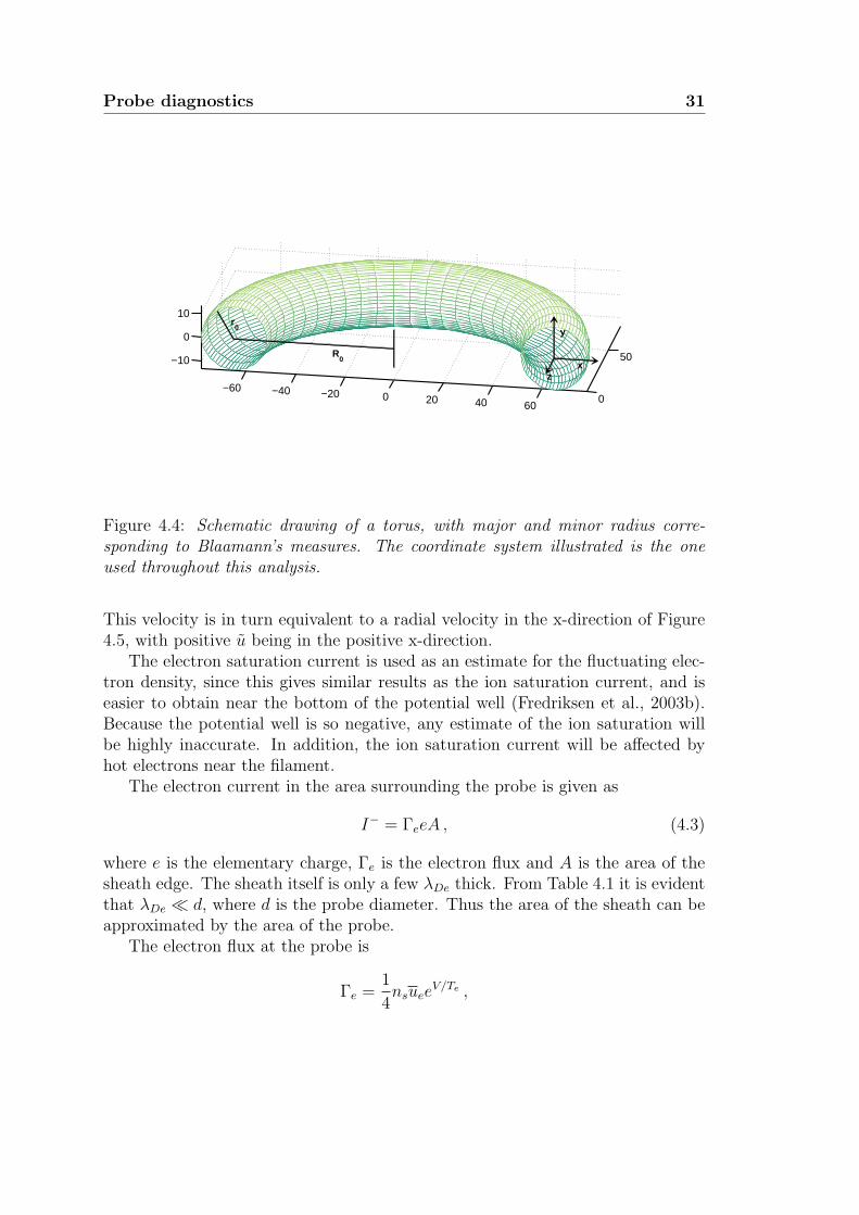
z
Figure 4.4: Schematic drawing of a torus, with major and minor radius corre-sponding to Blaamann’s measures. The coordinate system illustrated is the oneused throughout this analysis.
This velocity is in turn equivalent to a radial velocity in the x-direction of Figure4.5, with positive u being in the positive x-direction.
The electron saturation current is used as an estimate for the fluctuating elec-tron density, since this gives similar results as the ion saturation current, and iseasier to obtain near the bottom of the potential well (Fredriksen et al., 2003b).Because the potential well is so negative, any estimate of the ion saturation willbe highly inaccurate. In addition, the ion saturation current will be affected byhot electrons near the filament.
The electron current in the area surrounding the probe is given as
I− = ΓeeA , (4.3)
where e is the elementary charge, Γe is the electron flux and A is the area of thesheath edge. The sheath itself is only a few λDe thick. From Table 4.1 it is evidentthat λDe d, where d is the probe diameter. Thus the area of the sheath can beapproximated by the area of the probe.
The electron flux at the probe is
Γe =1
4nsuee
V/Te ,
32 The Blaamann experiment
5cm0
−5cm
y
xCH1
CH2
nB
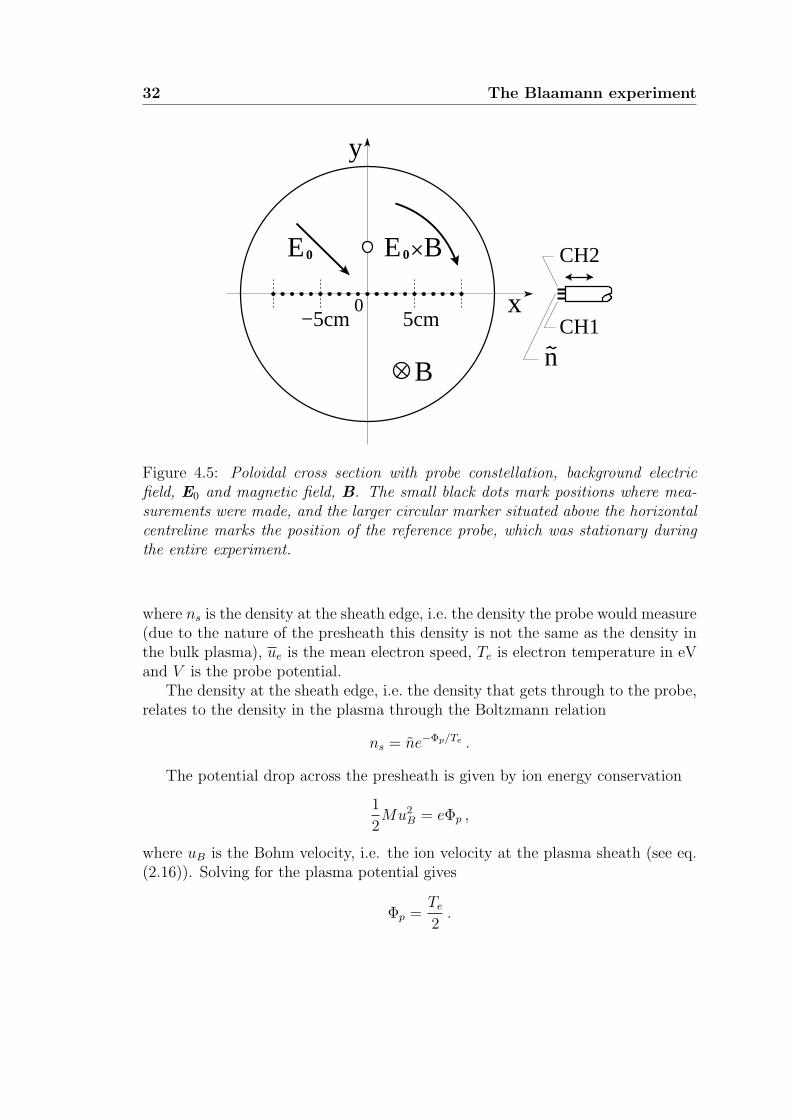
BEE0 0
Figure 4.5: Poloidal cross section with probe constellation, background electricfield, E0 and magnetic field, B. The small black dots mark positions where mea-surements were made, and the larger circular marker situated above the horizontalcentreline marks the position of the reference probe, which was stationary duringthe entire experiment.
where ns is the density at the sheath edge, i.e. the density the probe would measure(due to the nature of the presheath this density is not the same as the density inthe bulk plasma), ue is the mean electron speed, Te is electron temperature in eVand V is the probe potential.
The density at the sheath edge, i.e. the density that gets through to the probe,relates to the density in the plasma through the Boltzmann relation
ns = ne−Φp/Te .
The potential drop across the presheath is given by ion energy conservation
1
2Mu2
B = eΦp ,
where uB is the Bohm velocity, i.e. the ion velocity at the plasma sheath (see eq.(2.16)). Solving for the plasma potential gives
Φp =Te2.
Probe diagnostics 33
Thus the density at the sheath edge relates to the density in the main plasmathrough
ns = ne−1/2 ≈ 0.61n .
Assuming the electron velocity to have a Maxwellian distribution
f(u) = n( m
2πeT
)3/2
exp
(−mu
2
2eTe
)gives an average electron velocity of
ue =
(8eTeπme
)1/2
,
where me is the electron mass. me is known and Te is measured. With the temper-ature given in Table 4.1 this velocity is approximately ue ≈ 1.5× 10⁶ m/s. It hasbeen experimentally shown that even though the electron temperature fluctuates,with the low pressure that we have, these fluctuations do not significantly affectthe density (Fredriksen et al., 2003a). Therefore the electron temperature can beapproximated by a fixed value. In deriving the electron velocity we have assumedthat the electrons have three translational degrees of freedom.
Due to the highly limited electron motion across magnetic field lines, the cylin-drical probes can be treated like plane probes. This means that the effective surfacearea of the probe can be estimated as two times the cross section of the probe,i.e. the product of the diameter of the pins times their length. The circular endsection is so small that it is neglected here. Thus we have
A ≈ 2ld
which gives the final expression for the electron current. (Lieberman and Lichten-berg, 2005)
I− =1
4e
(8eTeπme
)1/2
2ldn exp
((V − Φp)
Te
).
Since the electron saturation current is the current that is measured when Φp = V ,the exponential disappears, and we have
I−sat = en
(eTe
2πme
)1/2
2ld . (4.4)
Solving for the fluctuating density n gives
n =I−sateld
(πme
2eTe
)1/2
. (4.5)
34 The Blaamann experiment
The fluctuating particle flux within the plasma is given as the product of thefluctuating density and the velocity.
Γx(x, t) = n(x, t)ux(x, t) (4.6)
The flux will also have a component n0(x)ux(x, t) due to the background density.However, this will on average be zero, and is therefore not investigated in thisstudy.
4.3 Plasma rotation and drifts
As mentioned a spatially averaged radial electric field component E0(r) gives riseto a rotation of the plasma column. Assuming a parabolic potential and a homo-geneous magnetic field given by its value near the centre of the device, one canestimate a rotation frequency Ω0/2π ≈ 8× 10³ Hz.
Estimating the individual rotation frequencies for the electrons and ions re-quires more consideration. The ion rotation frequency can be found from(
1 + 2Ω+
Ωci
)(Ω0
Ωci
− Ω+
Ωci
−(
Ω+
Ωci
)2)
=
(νi,nΩci
)2Ω+
Ωci
(4.7)
where the right hand side accounts for collisional friction due to the stationaryneutral gas, and the left hand side includes the effect of centrifugal forces onthe ions (Odajima, 1978). There would be a similar expression for the electronrotation frequency. However, given the low collision frequency, νen, compared tothe electron cyclotron frequency, ωce, found in Table 4.1, we can assume that theelectrons rotate with Ω0, and ignore friction and centrifugal forces.
The result of this difference in rotation frequency for the ions and electrons ischarge separation. Consider a localised plasma density enhancement or depletionat some finite radial position. Such a perturbation will be polarised due to thecharge separation, giving rise to electric fields. These electric fields will in turncause radial motion of the density perturbation, with depletions and enhancementsmoving in opposite directions.
In order to estimate the polarisation of a local plasma density perturbation,we need the difference in rotation frequency between the electrons and the ions.
∆Ω ≈ Ω0 − Ω+
which gives the relative displacement of the electrons with respect to the ions asapproximately
∆Ωtr
Plasma rotation and drifts 35
for a density perturbation δn at a position r at a time t > 0. The resulting electricfield is then
E ≈ te δn r∆Ω/ε0εr
where εr is the relative dielectric constant. Assuming that this can be estimatedusing the standard form for flute type slow plasma variations gives εr ≈ 1 +δnMc2µ0/B
2. For large perturbations this approaches εr ≈ δnMc2µ0/B2, and for
small perturbations we have εr ≈ 1. For the first case we find a radial velocity ofthe density perturbation
E/B ≈ trΩci∆Ω
independent of density, noting that the position varies with time, i.e. r = r(t). Inthe other limit we find
E/B ≈ tr δΩ2pi ∆Ω/Ωci
with δΩ2pi ≡ δne2/Mε0. Taking a perturbation δn/n ≈ 0.1 at a position x =
50 mm, we find εr ≈ 300, so the first case is relevant in the central parts of theplasma.
Using the parameters from Table 4.1 we find that both Ω0/Ωci 1 andνi,n/Ωci 1, indicating that the difference in rotation velocities for the elec-trons and the ions has a small contribution to the azimuthal current. However,the polarisation of a localised density perturbation can become important as itincreases with time.
To estimate this polarization we make the series expansion from the solutionof (4.7) to find
Ω+ ≈ Ω0 − Ω20/Ωci − Ω0(νi,n/Ωci)
2
givingΩci∆Ω ≈ Ω2
0 + ΩciΩ0(νi,n/Ωci)2
where the last term is small with parameters from Table 4.1. We therefore have
E/B = dr/dt ≈ trΩ20
with solution
r(t) = a exp
(1
2Ω2
0t2
)where a = r(0). This result indicates that a density perturbation can propagatesignificant radial distances during one rotation of the plasma column. In a fixedframe, the density perturbation will appear to follow a spiralling orbit. Also the∇B-gradient drift will contribute to the polarisation of a local plasma densityenhancement or depletion. To estimate the relative magnitude of the two polari-sations we compare the ∇B-velocity ≈ 0.6×10² m s−1 with r∆Ω ≈ 2.5×10² m s−1,
36 The Blaamann experiment
where we used R ≈ R0 for estimating the ∇B-velocity and r ≈ 50 mm for the dif-ferential rotation velocity. Other parameters were taken from Table 4.1. The twopolarisation effects seem to be of the same order of magnitude, but the ion ∇B-drift is in the positive y-direction on both the low and high magnetic field sides,and is therefore partially compensated by the plasma rotation. The polarisationdue to the differential rotation gives a drift that is always in the radial direction.We also note that a collisional drag will reduce the effect of the ∇B-gradient drift,while it will increase the differential rotation, see (4.7).
The radial drift deduced from these arguments come in addition to the bulkplasma rotation. If we follow a blob moving in the plasma column, it will follow a“spiral-like” orbit in the laboratory frame of reference.
4.4 Fluctuating velocities
In the following we identify the fluctuating plasma velocity component ⊥ B asE × B/B2, where we ignore polarisation drifts to the accuracy 〈ω〉/Ωci ≈ 10−3.For homogeneous magnetic fields and electrostatic fluctuations we have
∇ ·(E×B
)B2
= −∇ ·(∇φ×B
)B2
= 0 .
For the present case, however, we have B = B(r) so that ∇ · E×B/B2 6= 0, andthe plasma flow is slightly compressible. These velocities should be compared togradient and curvature drifts. We will find that root-mean-square E×B/B2-driftsare largest by about an order of magnitude. All these velocities are, however, smallcompared to the sound speed, see Table 4.1.
With our set-up and the parameters given in Table 4.1 we can estimate thevelocities associated with ∇B- and curvature drifts. The common factor in thetwo drift velocities is
∇BB
= − R
R2= − 1
Rr ≈ −1.53r ,
with magnitude in m−1. The curvature drift is given by equation (2.13), and for anelectron this would be approximately UDC ≈ 50 m/s directed downwards. Equiv-alently for the ∇B-drift, assuming the perpendicular velocity U⊥ is comparableto the average electron velocity is approximately U∇B ≈ 64 m/s, also directeddownwards for electrons. We will later find a fluctuating velocity with rms value∼ 500 m/s. As a reference we have Cs ≈ 104 m/s.
Chapter 5
Methods
In analysing the radial flux data from the Blaamann experiment we looked at anumber of different aspects and features of the datasets. The data files containsix variables, where two are derived (velocity and flux), and the other four areraw data (measurements of floating potentials and saturation currents). The mainfocus of this study is to investigate the nature of the plasma transport withinBlaamann by looking at the density, velocity and flux fluctuations in the plasmacolumn.
5.1 The probability density function
The measured time series by themselves are difficult to interpret directly. In orderto get an overall impression of the data we estimated the respective probabilitydensity functions (PDF) of the flux, velocity and density. This was done by group-ing the data into bins, and counting the number of observations within each bin,just like one would make a histogram. In order to normalise the function, thecounter for each bin was divided by both the total number of data points and thesize of the bin, thus ensuring that the area under the graph is equal to one.
We have five datasets for almost every position, with four sets for positions0 cm and -1 cm. In addition, one of the sets recorded for position -1 cm had tobe eliminated, due to some disturbance occurring during the first 2 ms of data.The PDF of each variable was estimated by grouping all the sets together into onelong time series and estimating the PDF for each position. This means that eachPDF is estimated from 50.000 points (40.000 for probe position x = 0 cm, and30.000 for x = −1 cm). The PDF is estimated for all positions, giving a set of 19functions showing how the distribution changes with probe position. The PDF ineach position is normalised individually.
A joint PDF for the velocity and the density was also found, in order to il-
38 Methods
lustrate how these two quantities relate. This was done similarly to the ordinaryPDFs, but corresponding data points from density measurements and velocitymeasurements were investigated simultaneously. Each event would then fall withina square of a grid where density values were along the x-axis and velocity valuesalong the y-axis. The result is then equivalent to a three dimensional histogram.
5.1.1 Theoretical model for the local particle flux
Assuming that the individual components that make up the flux signal, i.e. thedensity and velocity, are Gaussian in nature, Carreras et al. (1996) have deduced atheoretical joint distribution function for the fluctuating density and the velocitysignals.
f(n, ur) =1
2π
√1− γ2
WuWn
exp
[−(
u2r
2W 2u
+n2
2W 2n
+ γurn
WnWu
)](5.1)
Wu and Wn are the standard deviations of the velocity and density respectively, inthe absence of correlation. γ is the signed correlation between density and velocity,which means |γ| < 1. By introducing Γ = nur it can be shown that (5.1) gives thefollowing theoretical distribution for the fluctuation-induced turbulent flux.
p(Γ) =1
π
√1− γ2
WuWn
K0
(|Γ|
WuWn
)exp
(−γ Γ
WuWn
)(5.2)
K0 is the modified Bessel function of the second kind. γ will be estimated fromthe correlation coefficient for density and velocity for each position. Wu and Wn
are taken to be equal to σn and σu, i.e. the respective standard deviations of theexperimentally obtained density and velocity.
We intend to test the results of this model against the PDFs of flux obtainedfrom the experimental data.
5.2 Moments
Describing my data more quantitatively than a PDF requires calculating the lowerorder moments, thus finding specific numbers to describe the shape of the distri-butions. We will concentrate on the first four moments, as they are the ones thatare most easily interpreted and understood.
The first moment is the mean, µ, approximated as
µ = 〈x〉 =1
N
N∑i=1
xi (5.3)
Moments 39
for a dataset consisting of N measurements, where xi denotes the ith data point.The mean will only tell around which value the time series oscillates over the courseof the entire series. A standard normal distribution has 〈x〉 = 0.
The higher order central moments are given as
µn = 〈(x− 〈x〉)n〉 (5.4)
and are all centred around the sample mean.The second moment is the biased variance. This is related to the width of the
corresponding PDF, thus giving the spread of the data around the mean.
µ2 = σ2 = 〈(x− 〈x〉)2〉 (5.5)
For a random Gaussian process σ can take any value.Variance can be normalised by dividing by 〈x〉2, making σ2 dimensionless,
whereas the estimated mean is the only moment we cannot normalise. 〈x〉 willtherefore be in arbitrary units, while the higher order moments are dimensionless.
The third moment is the skewness, which indicates if and how a distributionof numbers may be skewed compared to the mean. If the distribution is perfectlysymmetric the skewness will be zero, as is the case for a Gaussian random process.If the left tail of the distribution is more pronounced than the right tail, theskewness is said to be negative, and similarly if the right tail is more pronouncedthe skewness is considered to be positive. The expression given underneath isnormalized with respect to the standard deviation. A large skewness indicates aclear deviation from the Gaussian distribution.
S =µ3
µ3/22
=〈(x− 〈x〉)3〉〈(x− 〈x〉)2〉3/2
(5.6)
The fourth moment is the kurtosis, and is given beneath in its normalizedform. It is a measure of how tall and slim or alternatively how short and wide thedistribution is compared to the normal distribution. In addition, it is a measureof the weight of the tails. A set of data that are have a Gaussian distributionwill have a normalized kurtosis of three. A kurtosis of less than three indicates adistribution that is wider and shorter than the normal distribution and that hasless heavy tails, whereas a kurtosis of more than three is indicative of a distributionthat is more peaked and has longer tails than the normal.
K =µ4
µ22
=〈(x− 〈x〉)4〉〈(x− 〈x〉)2〉2
(5.7)
A finite database can only provide an estimate for averages, not the true val-ues. With the large database available at each spatial position we can ignore this
40 Methods
uncertainty and assume that for instance (5.3) is an exact relation for a finite butlarge N -value.
Consider a random variable x and assume that you have found an estimate1N
∑Nj=1 xj for the average µ ≡ 〈x〉. The error e on the estimate is given as
e ≡
⟨(〈x〉 − 1
N
N∑j=1
xj
)2⟩.
We find
e = 〈x〉2 +1
N2
⟨(N∑j=1
xj
)2⟩− 2
⟨〈x〉 1
N
N∑j=1
xj
⟩.
The last sum is easy: each term in the sum becomes 〈x〉 and we have N of these,so we find all in all −2〈x〉2 for this term. The second term is written as
1
N2
N∑k=1
N∑j=1
〈xjxk〉 .
The double sum contains two sorts of terms: N terms where j = k and N(N − 1)terms where j 6= k. In the former case we have
〈x2j〉 = 〈x2〉
for each term, in the latter case we find
〈xjxk〉 = 〈xj〉〈xk〉 = 〈x〉2 .
Consequently we have
e = 〈x〉2 +1
N2(N〈x2〉+N(N − 1)〈x〉2)− 2〈x〉2
giving
e =1
N(〈x2〉 − 〈x〉2) .
We have e→ 0 for N →∞ as expected, in such a way that the root-mean-squareerror decreases as 1/
√N . The discussion can be extended to other averages.
5.2.1 Skewness-kurtosis relations
In order to discuss the possibility for a systematic relation between the skewnessand the kurtosis of the plasma flux signal we begin by introducing a simple two-level model, where we assume that the flux is “burst-like”, i.e. it is either vanishing
Moments 41
or it assumes a constant positive value γ > 0 in a short time interval. This meansthat the time variation of the flux event has a so called “top-hat” shape. Thetemporal duration of the flux event ∆τ is finite, so Gaussian or exponential pulses,for instance, are excluded. The random process is assumed to be time stationary,and the probability for encountering a plasma burst at some position is constant intime. At some fixed position at any given time it is assumed that the probabilityfor being in the interval ∆τ is 0 ≤ α ≤ 1. It is essential for the following discussionthat flux events do not overlap. This analysis addresses a plasma flux signal, sincethis is what we are concerned with here, but the arguments can just as easily beapplied for a density or velocity signal.
If we have a long time record of duration T , we have α = µ∆τ where µ ≈〈N〉/T is the number density of the appropriate flux-pulses in the record. Uncer-tainties arise due to end-effects, which can be made arbitrarily small by increasingT .
After averaging over different realisations, the probability density for the plasmaflux in this basic model is
P (Γ) = (1− α)δ(Γ) + αδ(Γ− γ) , (5.8)
where the first term accounts for the cases where the flux vanishes, i.e. at timeswhere no plasma burst is intercepted at the detection position, and the secondterm gives the probability distribution within a flux tube (the “top hat”). For thecase given by (5.8) we can obtain
〈Γm〉 = αγm
with m = 1, 2, 3, . . ., giving the average value
〈Γ〉 = αγ ,
the variance
σ2 ≡ 〈(Γ− 〈Γ〉)2〉 = α(1− α)γ2 ,
the skewness
S = α(1 + 2α− 3α2)γ3/σ3/2
and kurtosis
K = α(1− 4α + 6α2 − 3α3)γ4/σ4 ,
implying here the exact relation K = S 2 + 1 for any α. This can easily bedemonstrated by insertion. For this particular signal we have S = 0 when α =1/2.
42 Methods
The ”top-hat” model also gives a relation between normalized variance andskewness in the analytic form
σ2/〈Γ〉2 = 1 +1
2
(S 2 + S
√S 2 + 4
).
Note that this expression assumes 〈Γ〉 6= 0, so it will not apply for positions nearthe center of the plasma.
Generally it can be shown that K ≥ S 2 + 1 holds for any probability distri-bution, with the exception of PDFs with σ = 0 which are singular in the presentcontext. (We use here the definition where K = 3 for a Gaussian distribution.)More generally we actually have
K = AS 2 +B , (5.9)
where A and B are constants. The simple analytical model (5.8) and its generali-sations have been widely discussed in, e.g. studies of concentration fluctuations inturbulent environments (Jørgensen et al., 2010).
The model (5.8) can be generalised by allowing for a more general temporalform of the burst event containing a random parameter a with PDF P (a). Moreparameters can readily be included. We denote this form Ga(τ) for 0 ≤ τ ≤ ∆τand Ga(τ) = 0 otherwise. One example could be G(τ) = a sinp(πτ/∆τ) for 0 ≤τ ≤ ∆τ , where p is a fitting parameter. With this generalisation we find
P (Γ) = (1− α)δ(Γ) + α1
∆τ
∫ ∞0
∫ ∆τ
0
δ(Γ−Ga(τ))dτP (a)da , (5.10)
where it is assumed that a burst event is encountered at any time τ ∈ 0; ∆τ withequal probability. The previous results for 〈Γ〉, σ2, S and K are now generalised.We find, for instance,
〈Γm〉 = (α/∆τ)
∫ ∞0
∫ ∆τ
0
Ga(τ)mdτP (a)da .
The expression (5.10) can be formulated differently, but it turns out that this formis the most convenient here. For completeness, we might add that (except for thetop-hat signal) the distribution of amplitudes P (a) is not simply related to theprobability density of the signal amplitude, since a is the amplitude of a localmaximum. If we have the joint probability density of the flux and its two firstderivatives Γ(t), dΓ(t)/dt, d2Γ(t)/dt2 as PJ(Γ,Γ′,Γ′′) then P (a) =
∫∞0PJ(a,Γ′ =
0,Γ′′)dΓ′′.Extensions of the idealised model (5.8) have been presented by e.g. Jørgensen
et al. (2010), basically relying on generalisations included in (5.10). They found
Correlation functions and power spectra 43
that a parabolic relation like (5.9) remained but with A > 1 and B > 1. Thenumerical value of A and B depend on the structure shape Ga(τ).
Garcia (2012) discusses a model where pulses are superimposed randomly. Thepulses can in principle have infinite support, i.e. are not constrained to a finitetemporal or spatial domain. The position of one pulse or structure is there assumedto be independent of the position of all the others. This model will consequentlyhave the possibility of overlapping of two or more structures. Such models havebeen widely used for modelling random signals (Pecseli, 2000; Pecseli and Trulsen,1993). The model discussed by for instance (5.6) assumes that the basic pulses orstructures do not overlap: such a model seems much more reasonable here, since itis unlikely that one plasma burst can begin before the previous one has terminated.
5.3 Correlation functions and power spectra
A correlation function describes how two measurements made at different times t1and t2 are related, and measures how closely a dataset resembles itself at a latertime. It can also be used as a measure of predictability of a signal based on pastdata in the time series. It is defined as
C(t1, t2) ≡ 〈Y (t1)Y (t2)〉〈Y 2〉
, (5.11)
where σ2Y is the variance and 〈Y (t1)Y (t2)〉 is the autocovariance function of dataset
Y . Here the two events are from within the same time series. In such a case thefunction is called an autocorrelation function, i.e. it shows how a time series iscorrelated with itself.
The cross correlation function gives the correlation between two different timeseries, and can be considered as a measure of how well one measured quantity canbe used to predict the development of another. It is important to remember thatone might not know which variable is the cause and which is the effect. The crosscorrelation function is given as a similar expression as (5.11).
C(t1, t2) ≡ 〈X(t1)Y (t2)〉√〈X2〉〈Y 2〉
(5.12)
Assuming that we have a time stationary process, the above expressions canbe simplified by introducing τ which denotes the difference between t1 and t2, i.e.τ = t2 − t1.
CY Y (τ) =〈Y (t+ τ)Y (τ)〉
σ2Y
(5.13)
44 Methods
With the current data it is reasonable to assume that we have time stationaryevents, as there is little reason to assume that the PDF changes greatly throughoutthe time series.
Similarly for the cross correlation function we have
CXY (τ) =〈X(t)Y (t+ τ)〉√
σ2Xσ
2Y
. (5.14)
The discrete form of the above expression for the cross correlation function is
CXY (τ) =1n
∑n−τi=1 X(i)Y (i+ τ)√
σ2Xσ
2Y
. (5.15)
It is equivalent for the autocorrelation function.As we have several datasets for each probe position, it is convenient to combine
the results into one correlation function. The correct way of finding the average isgiven below, where the average of the covariance function between the two variablesX and Y , and the variance of X and Y all are found separately. The factor 1/5 isomitted from each average, as they cancel each other.
CXY (τ) =
∑5j=1
(1n
∑n−τi=1 X(i)Y (i+ τ)
)j√∑5
j=1 σ2X,j
∑5j=1 σ
2Y,j
(5.16)
Physically, a correlation function is a measure of a signals ability to interfere witheither itself (auto correlation) or with another (cross correlation), and for theauto correlation function this interference is always greatest at τ = 0. The crosscorrelation function can reach its maximum value for any τ depending on how thetwo signals are connected, and how the two probes are positioned according to oneanother. The correlation function yields physical information on e.g. time scalesof a process, or delay between two related processes.
In the current analysis it is most instructive to investigate how the physicalquantities, i.e. floating potential, density, velocity and flux are correlated withthe reference probe. The reference probe is situated a quarter of a revolutionfrom the positive probe positions, given that we follow the direction of the E ×B/B2-drift, and three quarters of a revolution from the negative probe positions.Any correlation between the reference probe and data from the moveable probeindicates that some structure with enhanced values for density or velocity (or both)has passed one of the probes and then the other, i.e. a coherent structure of somesort.
From the auto correlation function of a variable at a given position, the powerspectrum can be found by calculating the Fourier transform of said function. This
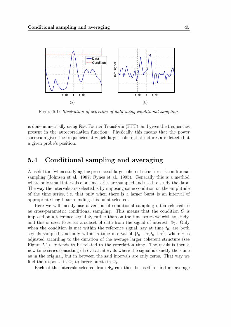
Conditional sampling and averaging 45
t−dt t t+dt
DataCondition
(a)
t−dt t t+dt
Dat
a si
gnal
(b)
Figure 5.1: Illustration of selection of data using conditional sampling.
is done numerically using Fast Fourier Transform (FFT), and gives the frequenciespresent in the autocorrelation function. Physically this means that the powerspectrum gives the frequencies at which larger coherent structures are detected ata given probe’s position.
5.4 Conditional sampling and averaging
A useful tool when studying the presence of large coherent structures is conditionalsampling (Johnsen et al., 1987; Øynes et al., 1995). Generally this is a methodwhere only small intervals of a time series are sampled and used to study the data.The way the intervals are selected is by imposing some condition on the amplitudeof the time series, i.e. that only when there is a larger burst is an interval ofappropriate length surrounding this point selected.
Here we will mostly use a version of conditional sampling often referred toas cross-parametric conditional sampling. This means that the condition C isimposed on a reference signal Φ1 rather than on the time series we wish to study,and this is used to select a subset of data from the signal of interest, Φ2. Onlywhen the condition is met within the reference signal, say at time t0, are bothsignals sampled, and only within a time interval of t0 − τ, t0 + τ, where τ isadjusted according to the duration of the average larger coherent structure (seeFigure 5.1). τ tends to be related to the correlation time. The result is then anew time series consisting of several intervals where the signal is exactly the sameas in the original, but in between the said intervals are only zeros. That way wefind the response in Φ2 to larger bursts in Φ1.
Each of the intervals selected from Φ2 can then be used to find an average
46 Methods
response, given as
Φca = 〈Φ2|C〉 , (5.17)
thus giving the conditionally averaged signal that is expected in Φ2, given that con-dition C is met in Φ1. This averaging over conditionally sampled subsets extractsthe coherent parts of the dataset, suppressing the uncorrelated parts. In otherwords, the turbulent fluctuations are averaged out, giving the average response inΦ2 to a spike in Φ1.
It is important to make sure that none of the intervals selected from either ofthe two datasets overlap, as that would mean that some measurements are sampledtwice in the conditional averaging. If intervals were to overlap there would be noguarantee that they are independent of each other. As we have already mentioned,we are already assuming that a model with no overlapping bursts is applicableto our data, thus it is not unreasonable to set this additional condition of onlysampling individual events that are clearly separated from the previous and thenext event within a time series.
Typically we will use conditions which are related to the standard deviation ofthe reference signal, e.g. C is Φ1 ≥ 1.5σ. We will spend some time investigatingthe effect of changing this condition for a higher or lower value.
The conditional averaging technique offers similar results as the cross correla-tion functions, which seems reasonable as they both in some way give a relationbetween a reference signal and another time series. The conditional average with|Φ1| > 1.5σ is a first approximation of the cross correlation function between thereference signal and the signal of interest. However, conditional averaging is alsosensitive to polarisation, as long as the conditional limit is set to be either a pos-itive or a negative number, and not both, i.e. if the condition is e.g. Φ1 > 1.5σ.Such a condition ensures that only large positive bursts are selected, ignoring allothers. This is useful when studying fluctuating data, as one is allowed to selectonly flow with enhanced positive speed, density, etc. If the condition is set to|Φ1| > 1.5σ however, the sensitivity to polarity disappears.
The conditional variance is defined as
Vcon =〈(Φ2 − 〈Φ2|C〉)2|C〉
〈(Φ2|C)2〉, (5.18)
and gives the level of reproducibility of the entire event, i.e. shape, position andtrajectory. Vcon can only take positive values between 0 and 1. A low variancemeans a high level of reproducibility, whereas a variance close to 1 means littleor no reproducibility. We use here the same definition of conditional variance asØynes et al. (1998).
Conditional sampling and averaging 47
5.4.1 Reference signals
The conditional sampling and averaging technique can be used to study any kindof physical quantity measured as a time series. In this study it would be possible touse it to investigate the velocity and density signals, as well as the flux. However,we will concentrate on the flux signal as it gives the most information with regardsto the transport of plasma within the tank. However, there is no limit on how manyconditions we can impose on the data when conditionally sampling fragments, thuswe can add conditions not only on the reference signal but also on the other signals.Since we will want to distinguish between transport in and out of the plasma,one additional condition will be Γ ≷ 0. Finally, distinguishing between densityenhancements and depletions and propagation in and out of the plasma, will beinteresting, and thus another condition will be u ≷ 0, or equivalently n ≷ 0.
The flux signal is the product of the fluctuating component of velocity anddensity. Therefore it seems likely that it will be more closely related to a referencesignal that is either a measure of velocity or density, rather than one that is a mea-sure of floating potential. As mentioned the electric field is directly proportionalto a velocity, and is also related to potential through
Ey = −∂φ∂y
.
In general we have that the potential is a function of space and time. Introducingthe coordinate ξ = y− u0t which gives position relative to the background motionwe can write the potential as φ(y− u0t, t). Differentiating this signal with respectto ξ is equivalent to differentiating with respect to y, since
∂ξ
∂y= 1 .
Thus we have∂φ
∂y=∂φ
∂ξ.
However, since we have floating potential φ as a time series, we only have the optionof differentiating with respect to time. As it turns out, this is not a problem.
∂φ
∂t= −u0
∂φ
∂ξ+∂φ(ξ, t′)
∂t′≈ −u0
∂φ
∂ξ= u0Eξ
Here we have assumed that ∂φ/∂t′ is small, i.e. implicitly we assume that the timeevolution is slow in the rotating frame of reference. The time derivative of φ isproportional to Ey as long as the fluctuations are small, meaning that we can treatu0 as a constant. Therefore we can assume that the time derivative of the signal

48 Methods
from the reference probe will be proportional to an electric field, and thus also toa velocity signal.
Ey ∼∂φ
∂t,
which will be assumed in the ensuing analysis.
Chapter 6
Results
The aim of this study is to investigate statistical properties of the data fromBlaamann, and to use this to infer a conclusion regarding the turbulent transport ofplasma within a simple magnetised torus. In this chapter our results are presentedand described.
6.1 The raw data
As mentioned these data consist of a number of sets collected at 19 differentpositions. Originally there were five sets for each position. However, for bothpositions 0 cm and -1 cm the final set is empty, i.e. no data. In addition, one setcollected at -1 cm had to be eliminated due to some disturbance causing very largeharmonic oscillations in the data during the first 2 ms of the set. Possibly the probewas situated in the middle of the plasma beam, thus causing the disturbance, butthere is really know way of knowing the cause for certain.
The raw data in itself offers little insight into the transport and motion ofplasma within the toroidal tank. However, a few samples of the data collectedat several different positions are included here for completeness, and in order toillustrate what the various time series look like (see Figure 6.1). It is clear thatthe signals fluctuate between much larger values nearer the centre, which is closerto the filament, with the greatest fluctuations found for x = −1 cm. The datacollected near the centre will most likely be very chaotic, and are not as valuableto our analysis as the datasets collected a little further out. However, they areuseful in illustrating the large amount of fluctuations occurring near the centre.Further out we have much smaller fluctuations. Note that there is not a symmetricdecrease in levels. The smallest fluctuations are found for x = −9 cm, with thecorresponding position on the outside demonstrating somewhat greater variation.
The density signal oscillates very quickly, whereas the velocity shows some signs
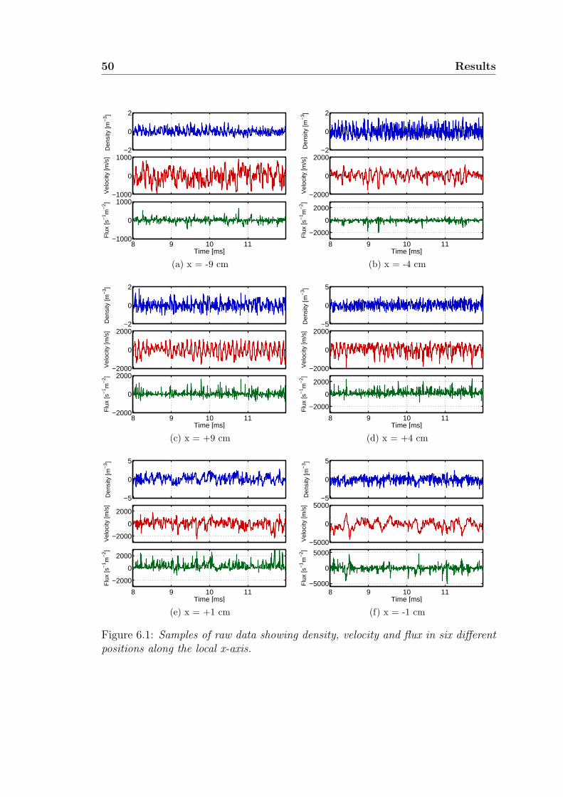
50 Results
−2
0
2D
ensi
ty [m
−3 ]
−1000
0
1000
Vel
ocity
[m/s
]
8 9 10 11−1000
0
1000
Time [ms]
Flu
x [s
−1 m
−2 ]
(a) x = -9 cm
−2
0
2
Den
sity
[m−
3 ]
−2000
0
2000
Vel
ocity
[m/s
]
8 9 10 11
−2000
0
2000
Time [ms]
Flu
x [s
−1 m
−2 ]
(b) x = -4 cm
−2
0
2
Den
sity
[m−
3 ]
−2000
0
2000
Vel
ocity
[m/s
]
8 9 10 11−2000
0
2000
Time [ms]
Flu
x [s
−1 m
−2 ]
(c) x = +9 cm
−5
0
5
Den
sity
[m−
3 ]
−2000
0
2000
Vel
ocity
[m/s
]
8 9 10 11
−2000
0
2000
Time [ms]
Flu
x [s
−1 m
−2 ]
(d) x = +4 cm
−5
0
5
Den
sity
[m−
3 ]
−2000
0
2000
Vel
ocity
[m/s
]
8 9 10 11
−2000
0
2000
Time [ms]
Flu
x [s
−1 m
−2 ]
(e) x = +1 cm
−5
0
5
Den
sity
[m−
3 ]
−5000
0
5000
Vel
ocity
[m/s
]
8 9 10 11−5000
0
5000
Time [ms]
Flu
x [s
−1 m
−2 ]
(f) x = -1 cm
Figure 6.1: Samples of raw data showing density, velocity and flux in six differentpositions along the local x-axis.
PDFs 51
of occasional harmonic bursts with a somewhat lower frequency, as can be seenfor instance in Figure 6.1d) in the interval 10-12 ms. Such bursts will be studiedmore closely using the conditional sampling technique.
It is also worth noticing the larger positive flux events in d) (x = 4 cm) atapproximately 8.5 ms, 10.5 ms and 11.5 ms with corresponding negative spikesin velocity and density. This indicates that we here have a density depletionmoving in the negative direction, i.e. inwards. Note that for negative positions anegative velocity corresponds to a velocity in the direction of the wall, i.e. outwards.Equivalently for x = −4 cm there are two clear negative spikes in the flux signal,one at 9.0 ms and one about 300 µs later, corresponding to negative spikes invelocity and positive spikes in density, which means these are density enhancementsmoving outwards.
6.2 PDFs
The first approach in studying the data from Blaamann was to find the probabilitydensity functions of the measured and derived quantities. The result of this isshown in Figure 6.2, where we have included the PDFs of velocity, flux and density,as well as the distribution we found for one for the probes measuring floatingpotential (channel 1). The equivalent distribution of the data from channel 2 isnot included as it is nearly identical to the one for channel 1 and thus would notcontribute with any additional insight.
As we can see, the floating potential has generally larger fluctuations for posi-tive x-values, i.e. on the outer side of the torus, with the widest PDFs at x = 7−8cm from the centre. There is also a slight asymmetry for the positive positions, witha skewness leaning towards positive values for the floating potential for positionsnear the wall, and towards negative values closer to the centre and the filament.For negative positions, the PDFs are more peaked, and also more symmetric.
The density distributions are rather varied for the different positions. For theinnermost positions the PDF is rather symmetric and peaked, with most fluctu-ations within an interval of ±1 m−3. However, as one moves towards the centre,the PDFs become increasingly skewed, leaning towards negative values. They arealso less peaked, with fluctuations occurring within a larger interval of densities.Nearing the filament, the skewness changes towards positive values. The distribu-tions also widen a great deal, indicating more large scale fluctuations of density inthis region. Nearing the outermost positions, the skewness changes again, leaningonce more towards negative values. For the outermost point the PDF is nearlysymmetric.
The PDFs for the velocity are all fairly symmetric, and there is less variation inwidth as well. The only exceptions are two of the positions closest to the filament,
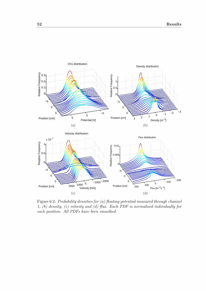
52 Results
−50
5
−5
0
5
0
0.1
0.2
0.3
Potential [V]
Ch1 distribution
Position [cm]
Rel
ativ
e F
requ
ency
(a)
−3−2−10123
−5
0
5
0
0.5
1
Density [m−3]
Density distribution
Position [cm]
Rel
ativ
e F
requ
ency
(b)
−2000−1000010002000
−5
0
5
0
0.5
1
x 10−3
Velocity [m/s]
Velocity distribution
Position [cm]
Rel
ativ
e F
requ
ency
(c)
−200−100
0100
200
−5
0
5
0
0.005
0.01
Flux [m−2s−1]
Flux distribution
Position [cm]
Rel
ativ
e F
requ
ency
(d)
Figure 6.2: Probability densities for (a) floating potential measured through channel1, (b) density, (c) velocity and (d) flux. Each PDF is normalised individually foreach position. All PDFs have been smoothed.
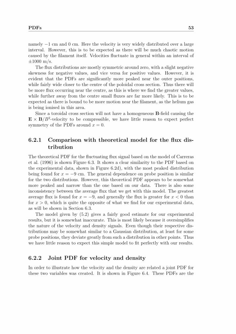
PDFs 53
namely −1 cm and 0 cm. Here the velocity is very widely distributed over a largeinterval. However, this is to be expected as there will be much chaotic motioncaused by the filament itself. Velocities fluctuate in general within an interval of±1000 m/s.
The flux distributions are mostly symmetric around zero, with a slight negativeskewness for negative values, and vice versa for positive values. However, it isevident that the PDFs are significantly more peaked near the outer positions,while fairly wide closer to the centre of the poloidal cross section. Thus there willbe more flux occurring near the centre, as this is where we find the greater values,while further away from the centre small fluxes are far more likely. This is to beexpected as there is bound to be more motion near the filament, as the helium gasis being ionised in this area.
Since a toroidal cross section will not have a homogeneous B-field causing theE × B/B2-velocity to be compressible, we have little reason to expect perfectsymmetry of the PDFs around x = 0.
6.2.1 Comparison with theoretical model for the flux dis-tribution
The theoretical PDF for the fluctuating flux signal based on the model of Carreraset al. (1996) is shown Figure 6.3. It shows a clear similarity to the PDF based onthe experimental data, shown in Figure 6.2d), with the most peaked distributionbeing found for x = −9 cm. The general dependence on probe position is similarfor the two distributions. However, this theoretical PDF appears to be somewhatmore peaked and narrow than the one based on our data. There is also someinconsistency between the average flux that we get with this model. The greatestaverage flux is found for x = −9, and generally the flux is greater for x < 0 thanfor x > 0, which is quite the opposite of what we find for our experimental data,as will be shown in Section 6.3.
The model given by (5.2) gives a fairly good estimate for our experimentalresults, but it is somewhat inaccurate. This is most likely because it oversimplifiesthe nature of the velocity and density signals. Even though their respective dis-tributions may be somewhat similar to a Gaussian distribution, at least for someprobe positions, they deviate greatly from such a distribution in other points. Thuswe have little reason to expect this simple model to fit perfectly with our results.
6.2.2 Joint PDF for velocity and density
In order to illustrate how the velocity and the density are related a joint PDF forthese two variables was created. It is shown in Figure 6.4. These PDFs are the
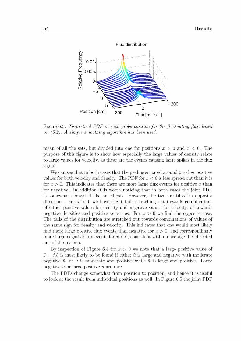
54 Results
−2000
200
−5
0
5
0
0.005
0.01
Flux [m−2s−1]
Flux distribution
Position [cm]
Rel
ativ
e F
requ
ency
Figure 6.3: Theoretical PDF in each probe position for the fluctuating flux, basedon (5.2). A simple smoothing algorithm has been used.
mean of all the sets, but divided into one for positions x > 0 and x < 0. Thepurpose of this figure is to show how especially the large values of density relateto large values for velocity, as these are the events causing large spikes in the fluxsignal.
We can see that in both cases that the peak is situated around 0 to low positivevalues for both velocity and density. The PDF for x < 0 is less spread out than it isfor x > 0. This indicates that there are more large flux events for positive x thanfor negative. In addition it is worth noticing that in both cases the joint PDFis somewhat elongated like an ellipsis. However, the two are tilted in oppositedirections. For x < 0 we have slight tails stretching out towards combinationsof either positive values for density and negative values for velocity, or towardsnegative densities and positive velocities. For x > 0 we find the opposite case.The tails of the distribution are stretched out towards combinations of values ofthe same sign for density and velocity. This indicates that one would most likelyfind more large positive flux events than negative for x > 0, and correspondinglymore large negative flux events for x < 0, consistent with an average flux directedout of the plasma.
By inspection of Figure 6.4 for x > 0 we note that a large positive value ofΓ ≡ nu is most likely to be found if either u is large and negative with moderatenegative n, or u is moderate and positive while n is large and positive. Largenegative n or large positive u are rare.
The PDFs change somewhat from position to position, and hence it is usefulto look at the result from individual positions as well. In Figure 6.5 the joint PDF
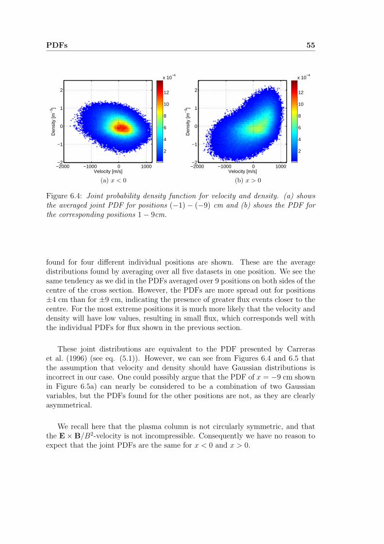
PDFs 55
Velocity [m/s]
Den
sity
[m−
3 ]
−2000 −1000 0 1000−2
−1
0
1
2
2
4
6
8
10
12
x 10−4
(a) x < 0Velocity [m/s]
Den
sity
[m−
3 ]
−2000 −1000 0 1000−2
−1
0
1
2
2
4
6
8
10
12
x 10−4
(b) x > 0
Figure 6.4: Joint probability density function for velocity and density. (a) showsthe averaged joint PDF for positions (−1)− (−9) cm and (b) shows the PDF forthe corresponding positions 1− 9cm.
found for four different individual positions are shown. These are the averagedistributions found by averaging over all five datasets in one position. We see thesame tendency as we did in the PDFs averaged over 9 positions on both sides of thecentre of the cross section. However, the PDFs are more spread out for positions±4 cm than for ±9 cm, indicating the presence of greater flux events closer to thecentre. For the most extreme positions it is much more likely that the velocity anddensity will have low values, resulting in small flux, which corresponds well withthe individual PDFs for flux shown in the previous section.
These joint distributions are equivalent to the PDF presented by Carreraset al. (1996) (see eq. (5.1)). However, we can see from Figures 6.4 and 6.5 thatthe assumption that velocity and density should have Gaussian distributions isincorrect in our case. One could possibly argue that the PDF of x = −9 cm shownin Figure 6.5a) can nearly be considered to be a combination of two Gaussianvariables, but the PDFs found for the other positions are not, as they are clearlyasymmetrical.
We recall here that the plasma column is not circularly symmetric, and thatthe E×B/B2-velocity is not incompressible. Consequently we have no reason toexpect that the joint PDFs are the same for x < 0 and x > 0.
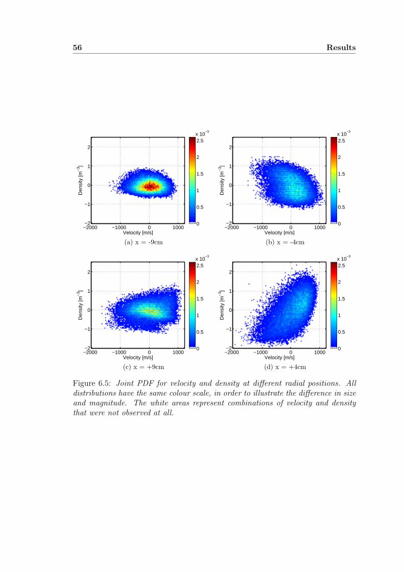
56 Results
Velocity [m/s]
Den
sity
[m−
3 ]
−2000 −1000 0 1000−2
−1
0
1
2
0
0.5
1
1.5
2
2.5x 10
−3
(a) x = -9cmVelocity [m/s]
Den
sity
[m−
3 ]
−2000 −1000 0 1000−2
−1
0
1
2
0
0.5
1
1.5
2
2.5x 10
−3
(b) x = -4cm
Velocity [m/s]
Den
sity
[m−
3 ]
−2000 −1000 0 1000−2
−1
0
1
2
0
0.5
1
1.5
2
2.5x 10
−3
(c) x = +9cmVelocity [m/s]
Den
sity
[m−
3 ]
−2000 −1000 0 1000−2
−1
0
1
2
0
0.5
1
1.5
2
2.5x 10
−3
(d) x = +4cm
Figure 6.5: Joint PDF for velocity and density at different radial positions. Alldistributions have the same colour scale, in order to illustrate the difference in sizeand magnitude. The white areas represent combinations of velocity and densitythat were not observed at all.
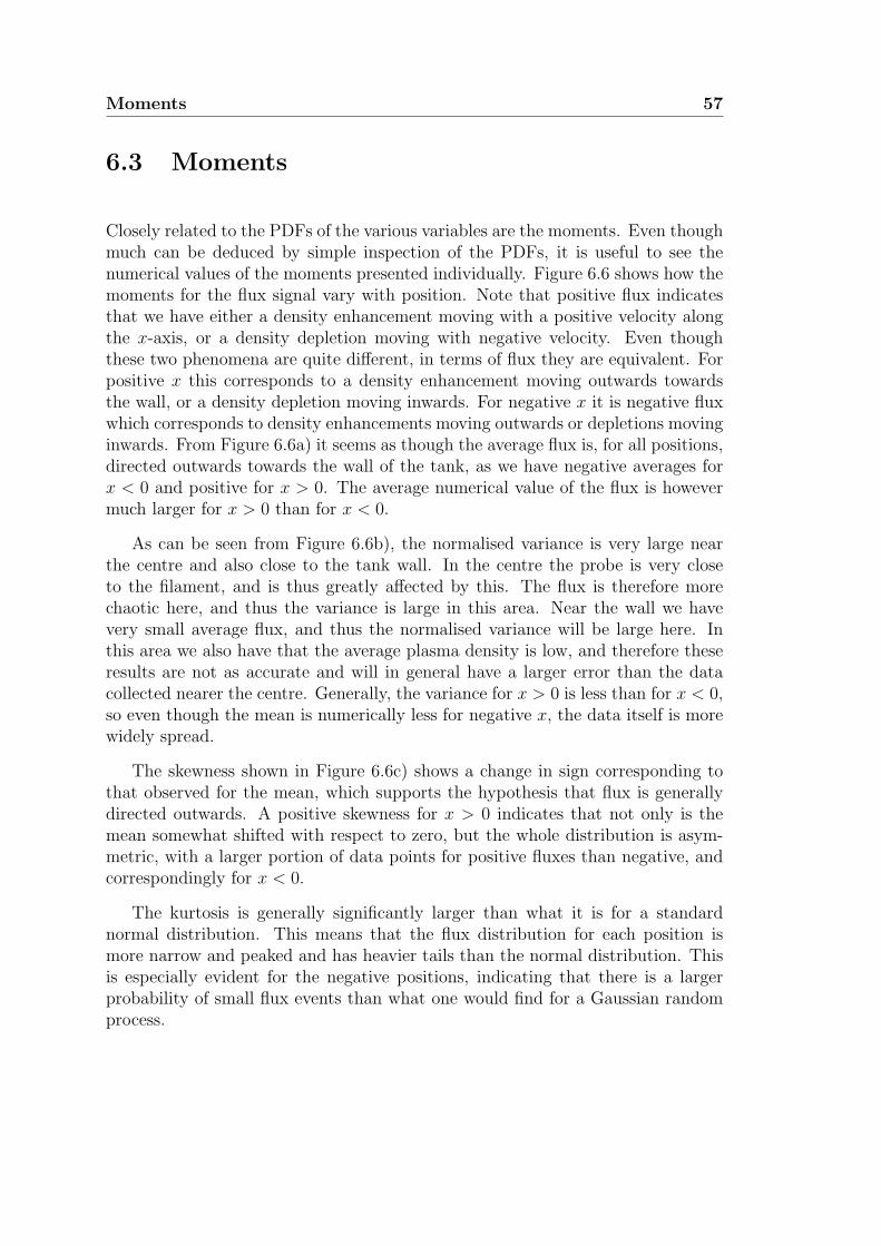
Moments 57
6.3 Moments
Closely related to the PDFs of the various variables are the moments. Even thoughmuch can be deduced by simple inspection of the PDFs, it is useful to see thenumerical values of the moments presented individually. Figure 6.6 shows how themoments for the flux signal vary with position. Note that positive flux indicatesthat we have either a density enhancement moving with a positive velocity alongthe x-axis, or a density depletion moving with negative velocity. Even thoughthese two phenomena are quite different, in terms of flux they are equivalent. Forpositive x this corresponds to a density enhancement moving outwards towardsthe wall, or a density depletion moving inwards. For negative x it is negative fluxwhich corresponds to density enhancements moving outwards or depletions movinginwards. From Figure 6.6a) it seems as though the average flux is, for all positions,directed outwards towards the wall of the tank, as we have negative averages forx < 0 and positive for x > 0. The average numerical value of the flux is howevermuch larger for x > 0 than for x < 0.
As can be seen from Figure 6.6b), the normalised variance is very large nearthe centre and also close to the tank wall. In the centre the probe is very closeto the filament, and is thus greatly affected by this. The flux is therefore morechaotic here, and thus the variance is large in this area. Near the wall we havevery small average flux, and thus the normalised variance will be large here. Inthis area we also have that the average plasma density is low, and therefore theseresults are not as accurate and will in general have a larger error than the datacollected nearer the centre. Generally, the variance for x > 0 is less than for x < 0,so even though the mean is numerically less for negative x, the data itself is morewidely spread.
The skewness shown in Figure 6.6c) shows a change in sign corresponding tothat observed for the mean, which supports the hypothesis that flux is generallydirected outwards. A positive skewness for x > 0 indicates that not only is themean somewhat shifted with respect to zero, but the whole distribution is asym-metric, with a larger portion of data points for positive fluxes than negative, andcorrespondingly for x < 0.
The kurtosis is generally significantly larger than what it is for a standardnormal distribution. This means that the flux distribution for each position ismore narrow and peaked and has heavier tails than the normal distribution. Thisis especially evident for the negative positions, indicating that there is a largerprobability of small flux events than what one would find for a Gaussian randomprocess.
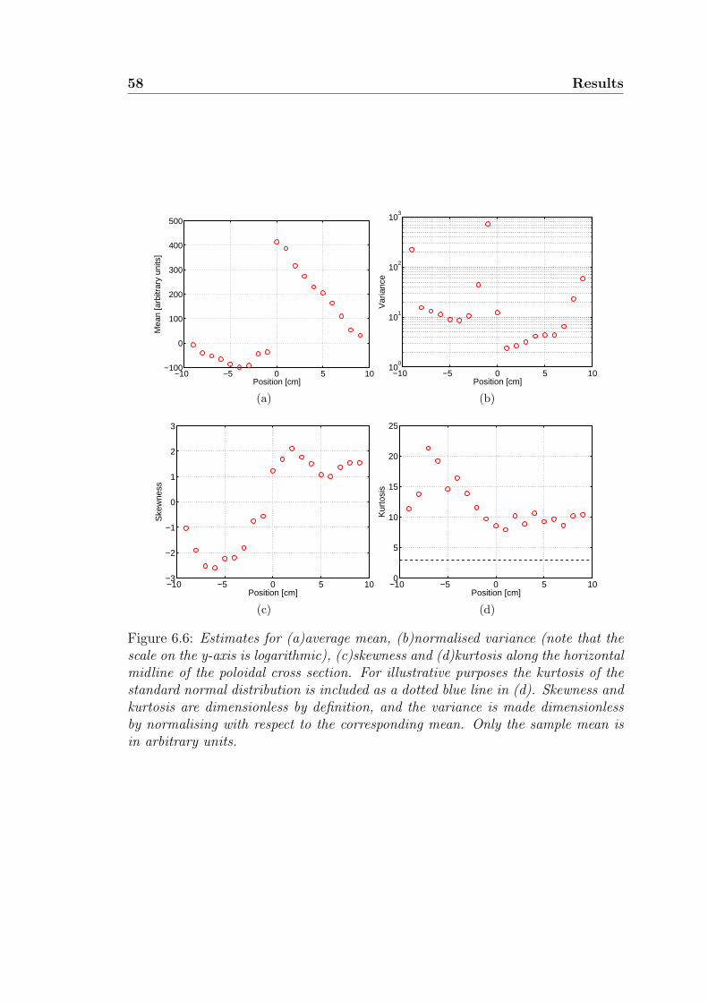
58 Results
−10 −5 0 5 10−100
0
100
200
300
400
500
Position [cm]
Mea
n [a
rbitr
ary
units
]
(a)
−10 −5 0 5 1010
0
101
102
103
Position [cm]V
aria
nce
(b)
−10 −5 0 5 10−3
−2
−1
0
1
2
3
Position [cm]
Ske
wne
ss
(c)
−10 −5 0 5 100
5
10
15
20
25
Position [cm]
Kur
tosi
s
(d)
Figure 6.6: Estimates for (a)average mean, (b)normalised variance (note that thescale on the y-axis is logarithmic), (c)skewness and (d)kurtosis along the horizontalmidline of the poloidal cross section. For illustrative purposes the kurtosis of thestandard normal distribution is included as a dotted blue line in (d). Skewness andkurtosis are dimensionless by definition, and the variance is made dimensionlessby normalising with respect to the corresponding mean. Only the sample mean isin arbitrary units.
Moments 59
−4 −2 0 2 40
5
10
15
20
25
30
Skewness
Kur
tosi
s
(a)
−4 −2 0 2 40
5
10
15
20
25
30
Skewness
Kur
tosi
s(b)
Figure 6.7: (a)Skewness/kurtosis relation with both data points from each datasetseparately (blue), and grouped according to position (red). The green curve is thefitted curve, and the blue curve is the curve corresponding to a two level model.(b) The same relation but including data from datasets of argon plasma (black),also recorded in an experiment conducted using Blaamann. The green curve is thefitted curve based on the original data from the helium plasma experiment, and theblue dashed curve corresponds to the two level model, and is the absolute theoreticalminimum of any data point. The black point in (0, 0) is a remnant from missingdata sets, and can be disregarded.
6.3.1 Skewness/kurtosis relation for plasma flux
In investigating the relation between skewness and kurtosis for the flux, both theoriginal data from this particular experiment was used, supplemented by data fromanother experiment conducted using Blaamann, but with argon plasma rather thanhelium. The experimental set-up for the argon experiment was somewhat different.About half the data was recorded with a low gas pressure (1.0× 10⁻⁴ mbar, whichis half of what we had for the helium plasma), and the rest with high pressure(1.0 × 10⁻³ mbar). In addition, measurements were made for several differentvalues of the toroidal field current, which ranged from 100 A up to 600 A. 23datasets exist for each configuration, with probes positioned similarly to what wasdone in the helium experiment.
The results using only our original data is shown in Figure 6.7a), where both theskewness and kurtosis of each individual set is included (marked as blue circles),as well as the resulting moments found when combining the individual sets intoone large set for each radial position (red circles). As indicated in Section 5.2.1, wemight expect to see some relation between the skewness and the kurtosis resembling
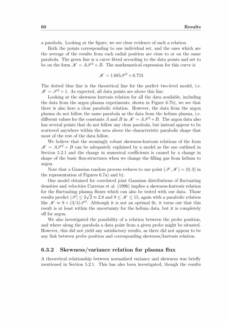
60 Results
a parabola. Looking at the figure, we see clear evidence of such a relation.Both the points corresponding to one individual set, and the ones which are
the average of the results from each radial position are close to or on the sameparabola. The green line is a curve fitted according to the data points and set tobe on the form K = AS 2 +B. The mathematical expression for this curve is
K = 1.685S 2 + 6.753
The dotted blue line is the theoretical line for the perfect two-level model, i.e.K = S 2 + 1. As expected, all data points are above this line.
Looking at the skewness kurtosis relation for all the data available, includingthe data from the argon plasma experiments, shown in Figure 6.7b), we see thatthere is also here a clear parabolic relation. However, the data from the argonplasma do not follow the same parabola as the data from the helium plasma, i.e.different values for the constants A and B in K = AS 2 +B. The argon data alsohas several points that do not follow any clear parabola, but instead appear to bescattered anywhere within the area above the characteristic parabolic shape thatmost of the rest of the data follow.
We believe that the seemingly robust skewness-kurtosis relations of the formK = AS 2 + B can be adequately explained by a model as the one outlined inSection 5.2.1 and the change in numerical coefficients is caused by a change inshape of the basic flux-structures when we change the filling gas from helium toargon.
Note that a Gaussian random process reduces to one point (S ,K ) = (0, 3) inthe representation of Figures 6.7a) and b).
One model obtained for correlated joint Gaussian distributions of fluctuatingdensities and velocities Carreras et al. (1996) implies a skewness-kurtosis relationfor the fluctuating plasma fluxes which can also be tested with our data. Thoseresults predict |S | ≤ 2
√2 ≈ 2.8 and 9 ≤ K ≤ 15, again with a parabolic relation
like K ≈ 9 + (3/4)S 2. Although it is not an optimal fit, it turns out that thisresult is at least within the uncertainty for the helium data, but it is completelyoff for argon.
We also investigated the possibility of a relation between the probe position,and where along the parabola a data point from a given probe might be situated.However, this did not yield any satisfactory results, as there did not appear to beany link between probe position and corresponding skewness/kurtosis relation.
6.3.2 Skewness/variance relation for plasma flux
A theoretical relationship between normalised variance and skewness was brieflymentioned in Section 5.2.1. This has also been investigated, though the results
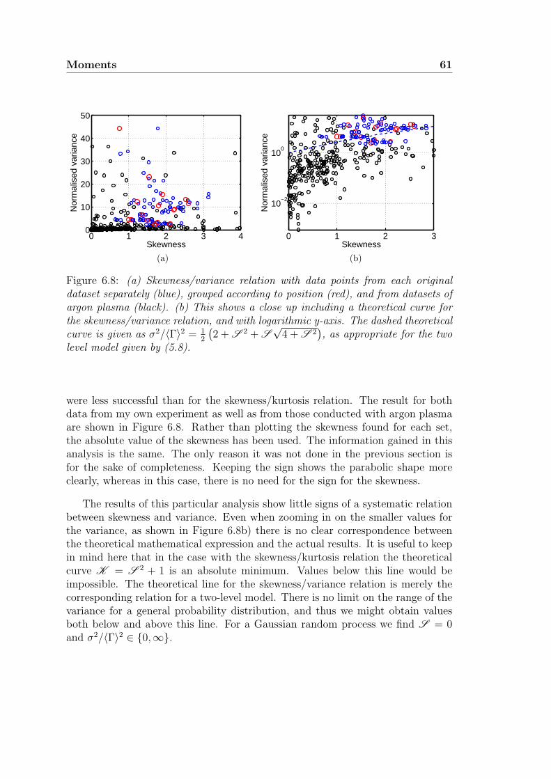
Moments 61
0 1 2 3 40
10
20
30
40
50
Skewness
Nor
mal
ised
var
ianc
e
(a)
0 1 2 3
10−2
100
Skewness
Nor
mal
ised
var
ianc
e(b)
Figure 6.8: (a) Skewness/variance relation with data points from each originaldataset separately (blue), grouped according to position (red), and from datasets ofargon plasma (black). (b) This shows a close up including a theoretical curve forthe skewness/variance relation, and with logarithmic y-axis. The dashed theoreticalcurve is given as σ2/〈Γ〉2 = 1
2
(2 + S 2 + S
√4 + S 2
), as appropriate for the two
level model given by (5.8).
were less successful than for the skewness/kurtosis relation. The result for bothdata from my own experiment as well as from those conducted with argon plasmaare shown in Figure 6.8. Rather than plotting the skewness found for each set,the absolute value of the skewness has been used. The information gained in thisanalysis is the same. The only reason it was not done in the previous section isfor the sake of completeness. Keeping the sign shows the parabolic shape moreclearly, whereas in this case, there is no need for the sign for the skewness.
The results of this particular analysis show little signs of a systematic relationbetween skewness and variance. Even when zooming in on the smaller values forthe variance, as shown in Figure 6.8b) there is no clear correspondence betweenthe theoretical mathematical expression and the actual results. It is useful to keepin mind here that in the case with the skewness/kurtosis relation the theoreticalcurve K = S 2 + 1 is an absolute minimum. Values below this line would beimpossible. The theoretical line for the skewness/variance relation is merely thecorresponding relation for a two-level model. There is no limit on the range of thevariance for a general probability distribution, and thus we might obtain valuesboth below and above this line. For a Gaussian random process we find S = 0and σ2/〈Γ〉2 ∈ 0,∞.

62 Results
6.4 Correlation functions
The correlation functions of the various variables would give an indication of thepresence of coherent structures. Any large correlation indicates the existence of astructure of some coherence, either in time or in space, and in some cases both.
6.4.1 Autocorrelation functions and power spectra
The autocorrelation functions for density, velocity and flux are presented in Figure6.9. Here we see that there is a clear periodicity in both density and velocity,though with less correlated regions near the centre. It also appears as though thedensity is more correlated for x < 0, while velocity is most correlated for x > 0.They seem to be fluctuating with the same frequency, which is confirmed by thepower spectra shown in Figure 6.10. Both have clear peaks for a frequency ofabout 10 kHz, which is very close to the estimated rotation frequency discussedin Section 4.3. Generally, both velocity and density have peaks for slightly lowerfrequencies for x > 0 than for x < 0, though the difference is only of about ∼ 1kHz.
Looking at the autocorrelation of the flux signal there appears to be morefluctuations, but with much lower correlation. Since the flux signal is the product ofthe density and the velocity we would expect to see at least a second order harmonicoscillation, and possibly also higher order harmonics as well. Turning to the powerspectrum of the flux shown in Figure 6.9c) we see in addition to the peak near 10kHz also significant peaks around 20 kHz. There are also some signs of a thirdharmonic for positions 7−9cm. As indicated by both the autocorrelation functionand the power spectrum of the flux, this signal appears to be more complex thanthe velocity and density signals.
A model consistent with the results in Figure 6.9 assumes that the fluctuat-ing density as well as electric field component have a large amplitude part witha very short correlation time, superimposed on an oscillating part with smalleramplitude. This corresponds to the background plasma rotating, combined withthe brief occurrence of coherent structures. The two parts seem independent. Thisargument will in principle apply to all x-positions.
6.4.2 Cross correlation
We investigated the cross correlation of the reference probe signal with signalsalong the x-axis for floating potential, density, velocity and flux. The results arepresented in Figure 6.11. In all cases we see a correlation for both positive andnegative positions, with somewhat more chaos near the central positions. Neither
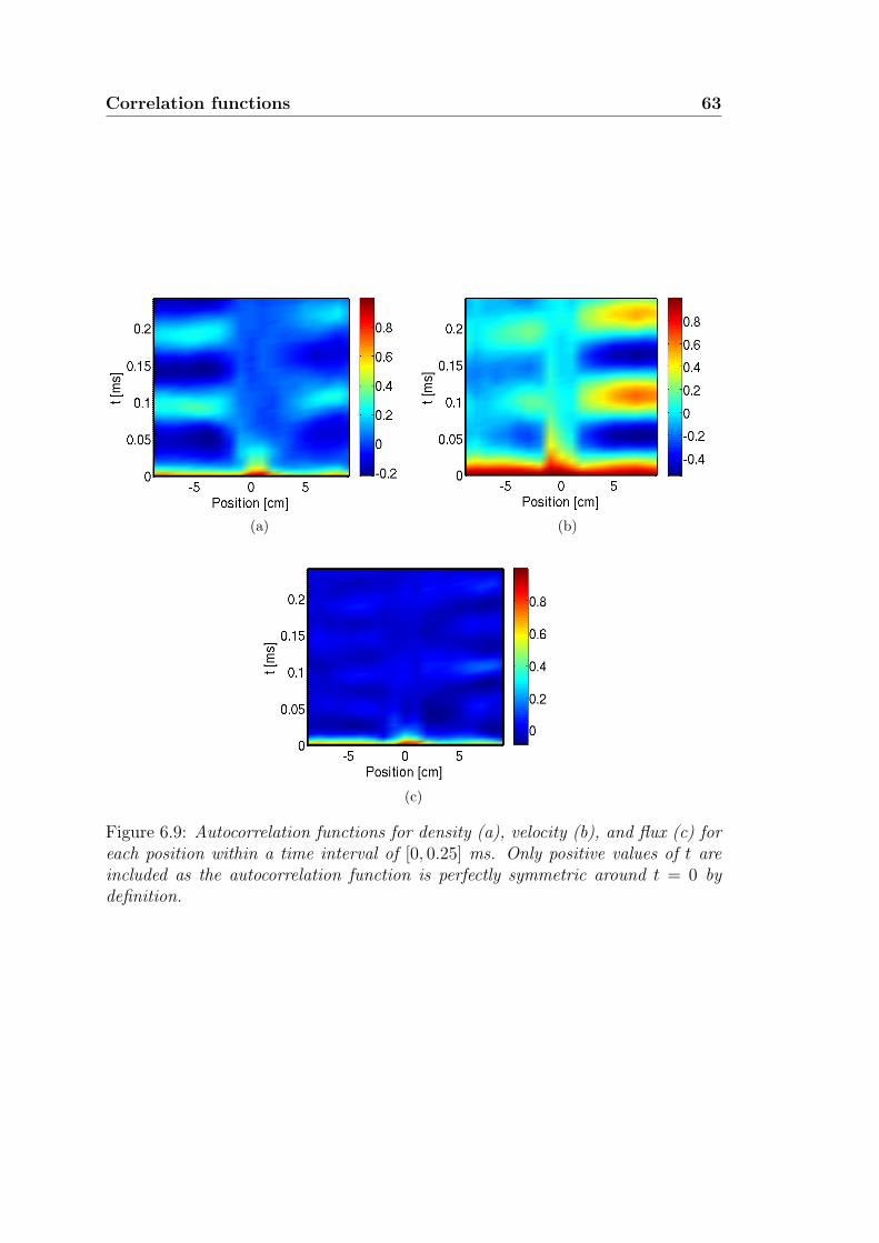
Correlation functions 63
(a) (b)
(c)
Figure 6.9: Autocorrelation functions for density (a), velocity (b), and flux (c) foreach position within a time interval of [0, 0.25] ms. Only positive values of t areincluded as the autocorrelation function is perfectly symmetric around t = 0 bydefinition.
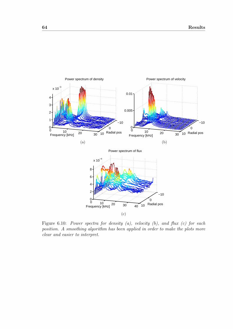
64 Results
−10
0
100 10 20 30
0
1
2
3
4
x 10−3
Radial pos
Power spectrum of density
Frequency [kHz]
(a)
−10
0
100 10 20 30
0
0.005
0.01
Radial pos
Power spectrum of velocity
Frequency [kHz]
(b)
−10
0
100 10 20 30 40
0
2
4
6
8
x 10−4
Radial pos
Power spectrum of flux
Frequency [kHz]
(c)
Figure 6.10: Power spectra for density (a), velocity (b), and flux (c) for eachposition. A smoothing algorithm has been applied in order to make the plots moreclear and easier to interpret.
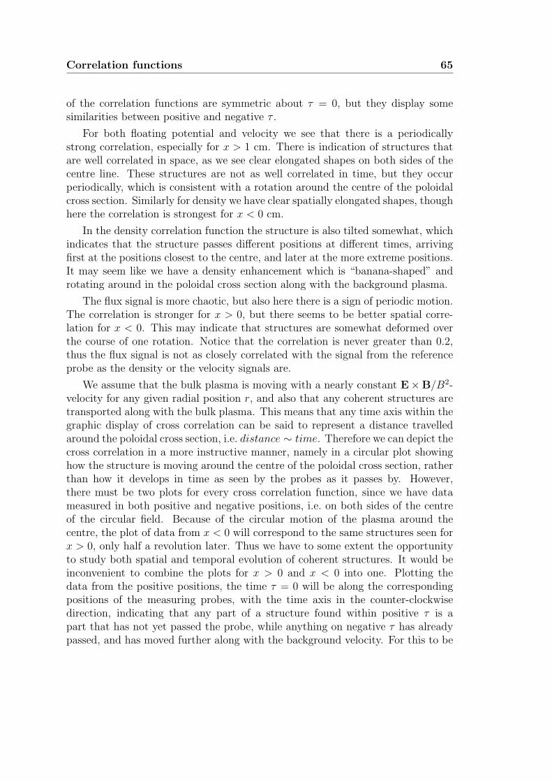
Correlation functions 65
of the correlation functions are symmetric about τ = 0, but they display somesimilarities between positive and negative τ .
For both floating potential and velocity we see that there is a periodicallystrong correlation, especially for x > 1 cm. There is indication of structures thatare well correlated in space, as we see clear elongated shapes on both sides of thecentre line. These structures are not as well correlated in time, but they occurperiodically, which is consistent with a rotation around the centre of the poloidalcross section. Similarly for density we have clear spatially elongated shapes, thoughhere the correlation is strongest for x < 0 cm.
In the density correlation function the structure is also tilted somewhat, whichindicates that the structure passes different positions at different times, arrivingfirst at the positions closest to the centre, and later at the more extreme positions.It may seem like we have a density enhancement which is “banana-shaped” androtating around in the poloidal cross section along with the background plasma.
The flux signal is more chaotic, but also here there is a sign of periodic motion.The correlation is stronger for x > 0, but there seems to be better spatial corre-lation for x < 0. This may indicate that structures are somewhat deformed overthe course of one rotation. Notice that the correlation is never greater than 0.2,thus the flux signal is not as closely correlated with the signal from the referenceprobe as the density or the velocity signals are.
We assume that the bulk plasma is moving with a nearly constant E×B/B2-velocity for any given radial position r, and also that any coherent structures aretransported along with the bulk plasma. This means that any time axis within thegraphic display of cross correlation can be said to represent a distance travelledaround the poloidal cross section, i.e. distance ∼ time. Therefore we can depict thecross correlation in a more instructive manner, namely in a circular plot showinghow the structure is moving around the centre of the poloidal cross section, ratherthan how it develops in time as seen by the probes as it passes by. However,there must be two plots for every cross correlation function, since we have datameasured in both positive and negative positions, i.e. on both sides of the centreof the circular field. Because of the circular motion of the plasma around thecentre, the plot of data from x < 0 will correspond to the same structures seen forx > 0, only half a revolution later. Thus we have to some extent the opportunityto study both spatial and temporal evolution of coherent structures. It would beinconvenient to combine the plots for x > 0 and x < 0 into one. Plotting thedata from the positive positions, the time τ = 0 will be along the correspondingpositions of the measuring probes, with the time axis in the counter-clockwisedirection, indicating that any part of a structure found within positive τ is apart that has not yet passed the probe, while anything on negative τ has alreadypassed, and has moved further along with the background velocity. For this to be
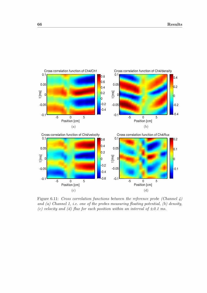
66 Results
(a) (b)
(c) (d)
Figure 6.11: Cross correlation functions between the reference probe (Channel 4)and (a) Channel 1, i.e. one of the probes measuring floating potential, (b) density,(c) velocity and (d) flux for each position within an interval of ±0.1 ms.
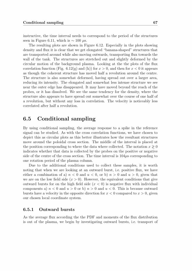
Conditional sampling 67
instructive, the time interval needs to correspond to the period of the structuresseen in Figure 6.11, which is ∼ 100 µs.
The resulting plots are shown in Figure 6.12. Especially in the plots showingdensity and flux it is clear that we get elongated “banana-shaped” structures thatare transported around while also moving outwards, transporting flux towards thewall of the tank. The structures are stretched out and slightly deformed by thecircular motion of the background plasma. Looking at the the plots of the fluxcorrelation function (Fig. 6.12(g) and (h)) for x > 0, and then for x < 0 it appearsas though the coherent structure has moved half a revolution around the centre.The structure is also somewhat deformed, having spread out over a larger area,reducing its intensity. The elongated and somewhat less intense structure we seenear the outer edge has disappeared. It may have moved beyond the reach of theprobes, or it has dissolved. We see the same tendency for the density, where thestructure also appears to have spread out somewhat over the course of one half ofa revolution, but without any loss in correlation. The velocity is noticeably lesscorrelated after half a revolution.
6.5 Conditional sampling
By using conditional sampling, the average response to a spike in the referencesignal can be studied. As with the cross correlation functions, we have chosen todepict this as circular plots as this better illustrates how the resultant structuresmove around the poloidal cross section. The middle of the interval is placed atthe position corresponding to where the data where collected. The notation x ≷ 0indicates whether that data is collected by the probes on the positive or negativeside of the centre of the cross section. The time interval is 104µs corresponding toone rotation period of the plasma column.
Due to the additional conditions used to collect these samples, it is worthnoting that when we are looking at an outward burst, i.e. positive flux, we haveeither a combination of a) n < 0 and u < 0, or b) n > 0 and u > 0, given thatwe are on the low field side (x > 0). However, the equivalent conditions that giveoutward bursts for on the high field side (x < 0) is negative flux with individualcomponents a) n < 0 and u > 0 or b) n > 0 and u < 0. This is because outwardbursts have a velocity in the opposite direction for x < 0 compared to x > 0, givenour chosen local coordinate system.
6.5.1 Outward bursts
As the average flux according the the PDF and moments of the flux distributionis out of the plasma, we begin by investigating outward bursts, i.e. transport of
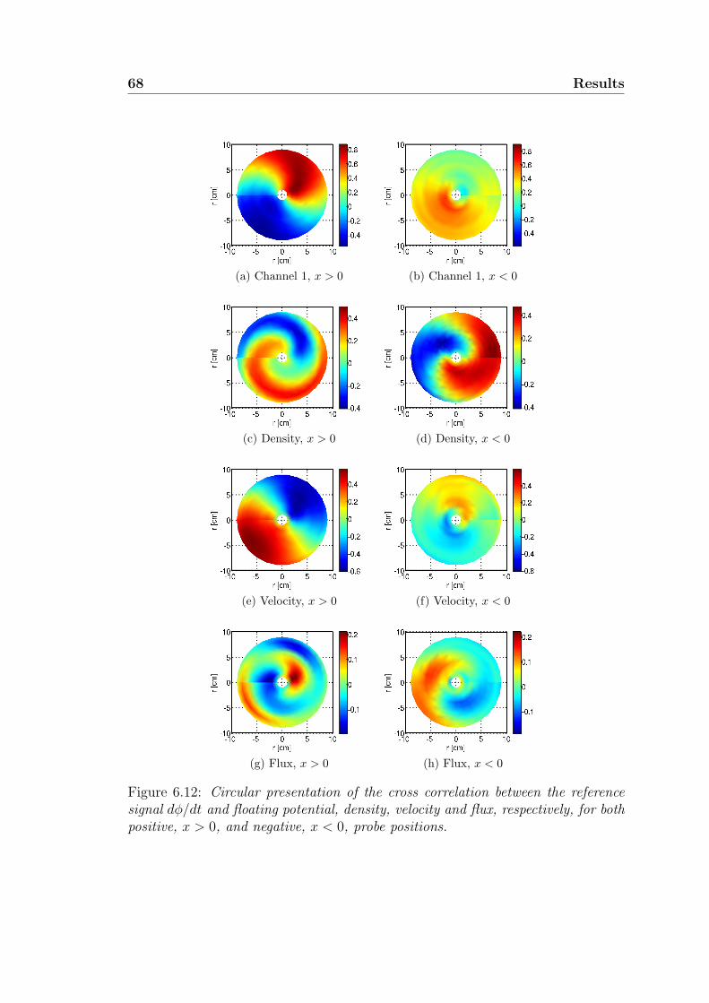
68 Results
(a) Channel 1, x > 0 (b) Channel 1, x < 0
(c) Density, x > 0 (d) Density, x < 0
(e) Velocity, x > 0 (f) Velocity, x < 0
(g) Flux, x > 0 (h) Flux, x < 0
Figure 6.12: Circular presentation of the cross correlation between the referencesignal dφ/dt and floating potential, density, velocity and flux, respectively, for bothpositive, x > 0, and negative, x < 0, probe positions.
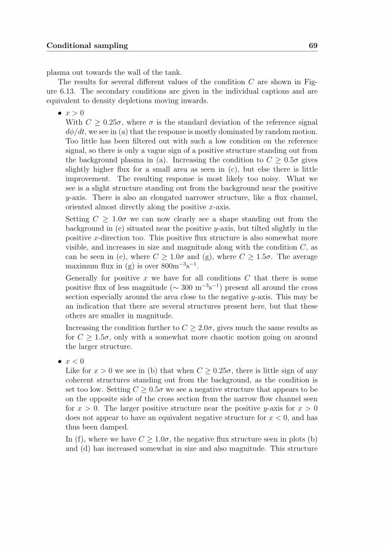
Conditional sampling 69
plasma out towards the wall of the tank.The results for several different values of the condition C are shown in Fig-
ure 6.13. The secondary conditions are given in the individual captions and areequivalent to density depletions moving inwards.
x > 0With C ≥ 0.25σ, where σ is the standard deviation of the reference signaldφ/dt, we see in (a) that the response is mostly dominated by random motion.Too little has been filtered out with such a low condition on the referencesignal, so there is only a vague sign of a positive structure standing out fromthe background plasma in (a). Increasing the condition to C ≥ 0.5σ givesslightly higher flux for a small area as seen in (c), but else there is littleimprovement. The resulting response is most likely too noisy. What wesee is a slight structure standing out from the background near the positivey-axis. There is also an elongated narrower structure, like a flux channel,oriented almost directly along the positive x-axis.
Setting C ≥ 1.0σ we can now clearly see a shape standing out from thebackground in (e) situated near the positive y-axis, but tilted slightly in thepositive x-direction too. This positive flux structure is also somewhat morevisible, and increases in size and magnitude along with the condition C, ascan be seen in (e), where C ≥ 1.0σ and (g), where C ≥ 1.5σ. The averagemaximum flux in (g) is over 800m−3s−1.
Generally for positive x we have for all conditions C that there is somepositive flux of less magnitude (∼ 300 m−3s−1) present all around the crosssection especially around the area close to the negative y-axis. This may bean indication that there are several structures present here, but that theseothers are smaller in magnitude.
Increasing the condition further to C ≥ 2.0σ, gives much the same results asfor C ≥ 1.5σ, only with a somewhat more chaotic motion going on aroundthe larger structure.
x < 0Like for x > 0 we see in (b) that when C ≥ 0.25σ, there is little sign of anycoherent structures standing out from the background, as the condition isset too low. Setting C ≥ 0.5σ we see a negative structure that appears to beon the opposite side of the cross section from the narrow flow channel seenfor x > 0. The larger positive structure near the positive y-axis for x > 0does not appear to have an equivalent negative structure for x < 0, and hasthus been damped.
In (f), where we have C ≥ 1.0σ, the negative flux structure seen in plots (b)and (d) has increased somewhat in size and also magnitude. This structure
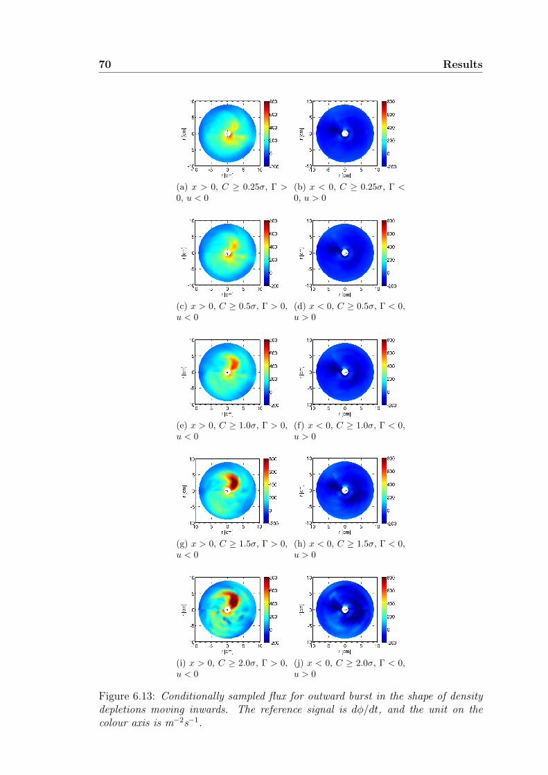
70 Results
(a) x > 0, C ≥ 0.25σ, Γ >0, u < 0
(b) x < 0, C ≥ 0.25σ, Γ <0, u > 0
(c) x > 0, C ≥ 0.5σ, Γ > 0,u < 0
(d) x < 0, C ≥ 0.5σ, Γ < 0,u > 0
(e) x > 0, C ≥ 1.0σ, Γ > 0,u < 0
(f) x < 0, C ≥ 1.0σ, Γ < 0,u > 0
(g) x > 0, C ≥ 1.5σ, Γ > 0,u < 0
(h) x < 0, C ≥ 1.5σ, Γ < 0,u > 0
(i) x > 0, C ≥ 2.0σ, Γ > 0,u < 0
(j) x < 0, C ≥ 2.0σ, Γ < 0,u > 0
Figure 6.13: Conditionally sampled flux for outward burst in the shape of densitydepletions moving inwards. The reference signal is dφ/dt, and the unit on thecolour axis is m−2s−1.
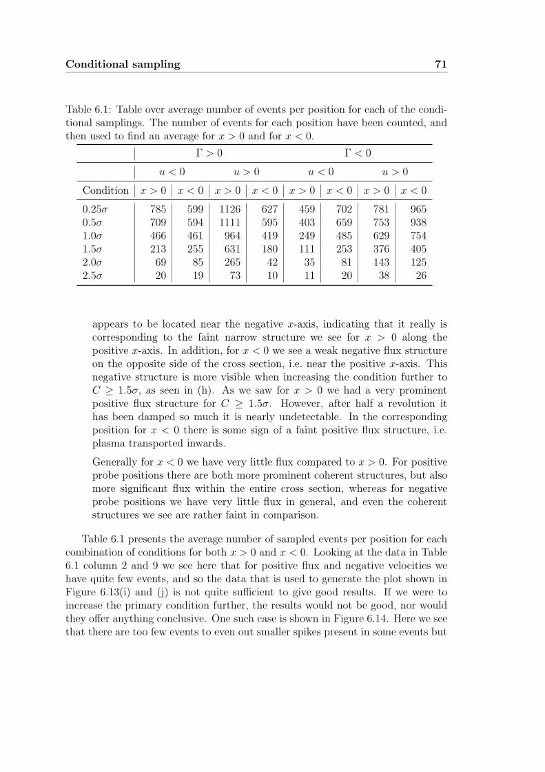
Conditional sampling 71
Table 6.1: Table over average number of events per position for each of the condi-tional samplings. The number of events for each position have been counted, andthen used to find an average for x > 0 and for x < 0.
Γ > 0 Γ < 0
u < 0 u > 0 u < 0 u > 0
Condition x > 0 x < 0 x > 0 x < 0 x > 0 x < 0 x > 0 x < 0
0.25σ 785 599 1126 627 459 702 781 9650.5σ 709 594 1111 595 403 659 753 9381.0σ 466 461 964 419 249 485 629 7541.5σ 213 255 631 180 111 253 376 4052.0σ 69 85 265 42 35 81 143 1252.5σ 20 19 73 10 11 20 38 26
appears to be located near the negative x-axis, indicating that it really iscorresponding to the faint narrow structure we see for x > 0 along thepositive x-axis. In addition, for x < 0 we see a weak negative flux structureon the opposite side of the cross section, i.e. near the positive x-axis. Thisnegative structure is more visible when increasing the condition further toC ≥ 1.5σ, as seen in (h). As we saw for x > 0 we had a very prominentpositive flux structure for C ≥ 1.5σ. However, after half a revolution ithas been damped so much it is nearly undetectable. In the correspondingposition for x < 0 there is some sign of a faint positive flux structure, i.e.plasma transported inwards.
Generally for x < 0 we have very little flux compared to x > 0. For positiveprobe positions there are both more prominent coherent structures, but alsomore significant flux within the entire cross section, whereas for negativeprobe positions we have very little flux in general, and even the coherentstructures we see are rather faint in comparison.
Table 6.1 presents the average number of sampled events per position for eachcombination of conditions for both x > 0 and x < 0. Looking at the data in Table6.1 column 2 and 9 we see here that for positive flux and negative velocities wehave quite few events, and so the data that is used to generate the plot shown inFigure 6.13(i) and (j) is not quite sufficient to give good results. If we were toincrease the primary condition further, the results would not be good, nor wouldthey offer anything conclusive. One such case is shown in Figure 6.14. Here we seethat there are too few events to even out smaller spikes present in some events but
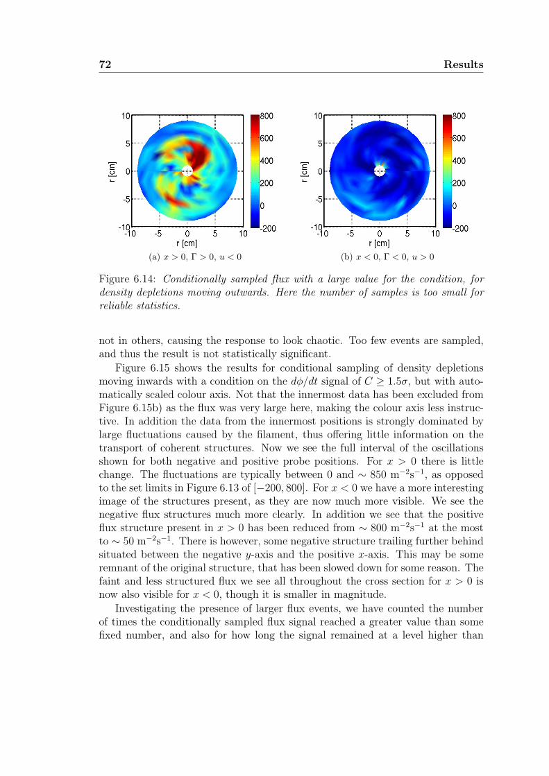
72 Results
(a) x > 0, Γ > 0, u < 0 (b) x < 0, Γ < 0, u > 0
Figure 6.14: Conditionally sampled flux with a large value for the condition, fordensity depletions moving outwards. Here the number of samples is too small forreliable statistics.
not in others, causing the response to look chaotic. Too few events are sampled,and thus the result is not statistically significant.
Figure 6.15 shows the results for conditional sampling of density depletionsmoving inwards with a condition on the dφ/dt signal of C ≥ 1.5σ, but with auto-matically scaled colour axis. Not that the innermost data has been excluded fromFigure 6.15b) as the flux was very large here, making the colour axis less instruc-tive. In addition the data from the innermost positions is strongly dominated bylarge fluctuations caused by the filament, thus offering little information on thetransport of coherent structures. Now we see the full interval of the oscillationsshown for both negative and positive probe positions. For x > 0 there is littlechange. The fluctuations are typically between 0 and ∼ 850 m−2s−1, as opposedto the set limits in Figure 6.13 of [−200, 800]. For x < 0 we have a more interestingimage of the structures present, as they are now much more visible. We see thenegative flux structures much more clearly. In addition we see that the positiveflux structure present in x > 0 has been reduced from ∼ 800 m−2s−1 at the mostto ∼ 50 m−2s−1. There is however, some negative structure trailing further behindsituated between the negative y-axis and the positive x-axis. This may be someremnant of the original structure, that has been slowed down for some reason. Thefaint and less structured flux we see all throughout the cross section for x > 0 isnow also visible for x < 0, though it is smaller in magnitude.
Investigating the presence of larger flux events, we have counted the numberof times the conditionally sampled flux signal reached a greater value than somefixed number, and also for how long the signal remained at a level higher than
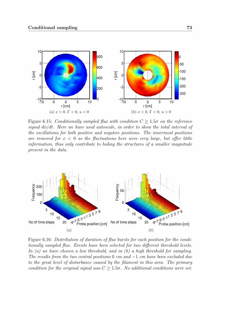
Conditional sampling 73
(a) x > 0, Γ > 0, u < 0 (b) x < 0, Γ < 0, u > 0
Figure 6.15: Conditionally sampled flux with condition C ≥ 1.5σ on the referencesignal dφ/dt. Here we have used autoscale, in order to show the total interval ofthe oscillations for both positive and negative positions. The innermost positionsare removed for x < 0 as the fluctuations here were very large, but offer littleinformation, thus only contribute to hiding the structures of a smaller magnitudepresent in the data.
(a) (b)
Figure 6.16: Distribution of duration of flux bursts for each position for the condi-tionally sampled flux. Events have been selected for two different threshold levels.In (a) we have chosen a low threshold, and in (b) a high threshold for sampling.The results from the two central positions 0 cm and −1 cm have been excluded dueto the great level of disturbance caused by the filament in this area. The primarycondition for the original signal was C ≥ 1.5σ. No additional conditions were set.
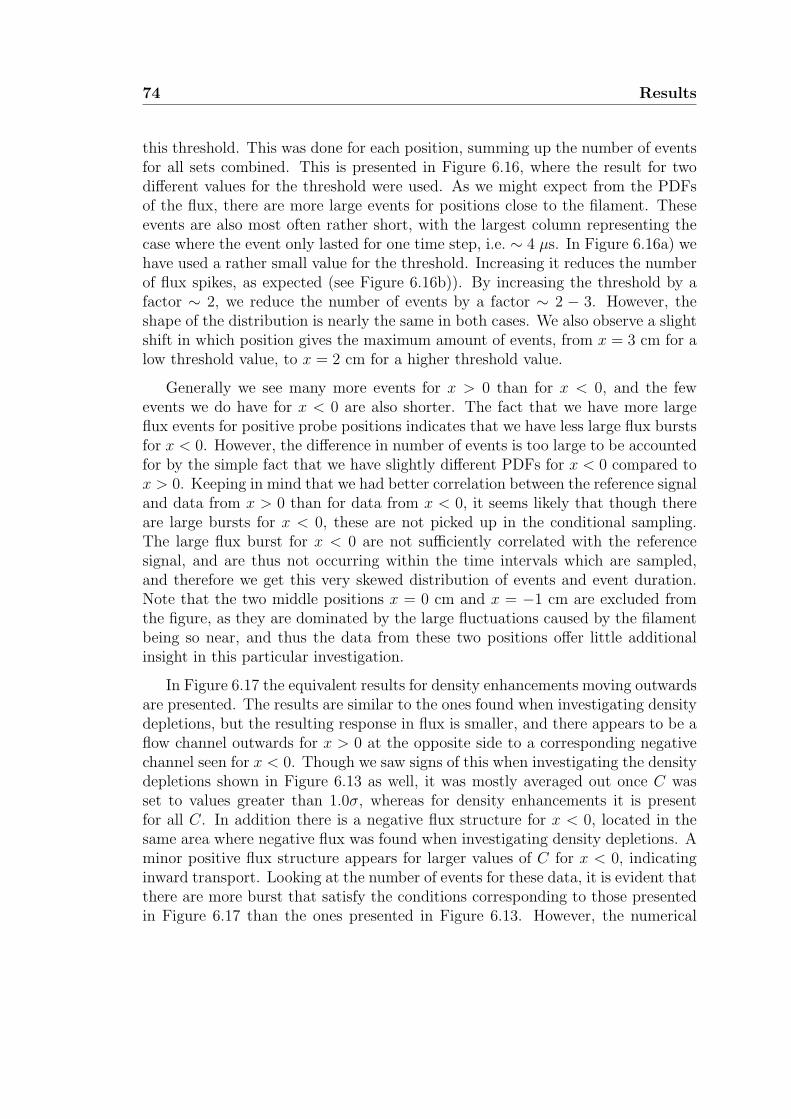
74 Results
this threshold. This was done for each position, summing up the number of eventsfor all sets combined. This is presented in Figure 6.16, where the result for twodifferent values for the threshold were used. As we might expect from the PDFsof the flux, there are more large events for positions close to the filament. Theseevents are also most often rather short, with the largest column representing thecase where the event only lasted for one time step, i.e. ∼ 4 µs. In Figure 6.16a) wehave used a rather small value for the threshold. Increasing it reduces the numberof flux spikes, as expected (see Figure 6.16b)). By increasing the threshold by afactor ∼ 2, we reduce the number of events by a factor ∼ 2 − 3. However, theshape of the distribution is nearly the same in both cases. We also observe a slightshift in which position gives the maximum amount of events, from x = 3 cm for alow threshold value, to x = 2 cm for a higher threshold value.
Generally we see many more events for x > 0 than for x < 0, and the fewevents we do have for x < 0 are also shorter. The fact that we have more largeflux events for positive probe positions indicates that we have less large flux burstsfor x < 0. However, the difference in number of events is too large to be accountedfor by the simple fact that we have slightly different PDFs for x < 0 compared tox > 0. Keeping in mind that we had better correlation between the reference signaland data from x > 0 than for data from x < 0, it seems likely that though thereare large bursts for x < 0, these are not picked up in the conditional sampling.The large flux burst for x < 0 are not sufficiently correlated with the referencesignal, and are thus not occurring within the time intervals which are sampled,and therefore we get this very skewed distribution of events and event duration.Note that the two middle positions x = 0 cm and x = −1 cm are excluded fromthe figure, as they are dominated by the large fluctuations caused by the filamentbeing so near, and thus the data from these two positions offer little additionalinsight in this particular investigation.
In Figure 6.17 the equivalent results for density enhancements moving outwardsare presented. The results are similar to the ones found when investigating densitydepletions, but the resulting response in flux is smaller, and there appears to be aflow channel outwards for x > 0 at the opposite side to a corresponding negativechannel seen for x < 0. Though we saw signs of this when investigating the densitydepletions shown in Figure 6.13 as well, it was mostly averaged out once C wasset to values greater than 1.0σ, whereas for density enhancements it is presentfor all C. In addition there is a negative flux structure for x < 0, located in thesame area where negative flux was found when investigating density depletions. Aminor positive flux structure appears for larger values of C for x < 0, indicatinginward transport. Looking at the number of events for these data, it is evident thatthere are more burst that satisfy the conditions corresponding to those presentedin Figure 6.17 than the ones presented in Figure 6.13. However, the numerical
Conditional sampling 75
value of the flux is generally greater for density depletions propagating inwards.
As mentioned in Section 5.4 we used a reference signal that is the time deriva-tive of the data from the reference probe, as this can be considered to be equivalentto an electric field signal, which would be better related to the flux than a float-ing potential signal. In Figure 6.18 is the resulting conditional average with theoriginal signal from the reference probe as a reference signal, with C ≥ 1.5σ ascondition for the reference probe signal, looking at density enhancements propa-gating outwards. Here we see less sign of coherent structures than we do in thecorresponding plots presented in Figure 6.17(g) and (h). We do not have the sameclear enhancement standing out from the background, like we did with dφ/dt asa reference, nor do we see the narrow flow channel as clearly. The resulting fluxis also even lower than the flux found using the time derivative of the referenceprobe. We also seem to find negative flux structures for x < 0 in different areas ofthe cross section, compared to what we found using dφ/dt as a reference signal.
6.5.2 Inward transport
Although the net average transport is out of the plasma column, we neverthelessfind occasional inward transport as well, see for instance the flux PDF in Figure6.2d). We can study such events as well using the conditional averaging technique,by changing the additional conditions to correspond to either density depletionsmoving outwards or enhancements moving inwards.
Figure 6.19 shows the results of conditional sampling and averaging with condi-tions corresponding to inward transport. For simplicity only a few different valuesof the main condition C are included here. However, what is interesting here isthat we find a flow channel of negative flux for both u < 0 and u > 0, corre-sponding to density enhancements flowing inwards and density depletions flowingoutwards (for x > 0). This channel of negative flux is slightly stronger in mag-nitude for u < 0, but the channel is wider for u > 0. In addition we also havethe coherent structure of positive flux flowing around along with the bulk plasma.For x < 0 we see clear signs of a corresponding positive flux channel at oppositesides to the negative channel seen for x > 0, though this structure appears to bestronger for u < 0 than u > 0, indicating greater magnitude for density depletionsmoving outwards. In addition we also see a faint negative structure that appearsto correspond to the positive structure visible for x > 0. Inward transport is ratherunexpected as it goes against what might be expected due to turbulent diffusionor blob transport.
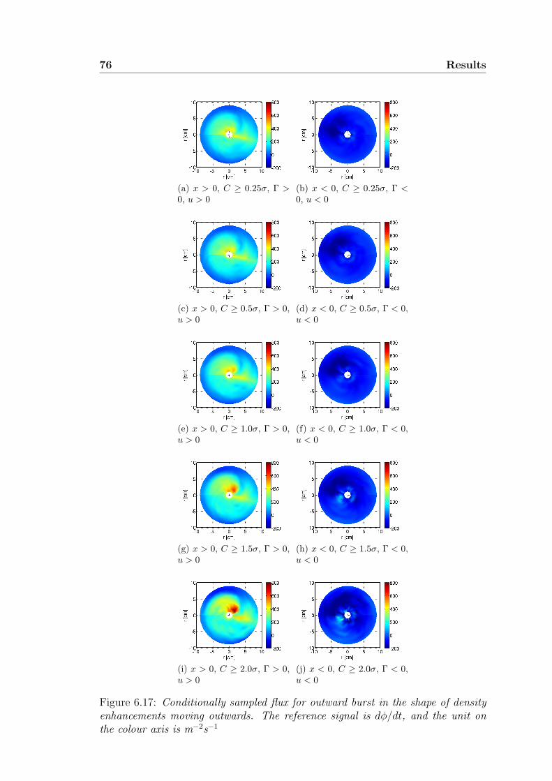
76 Results
(a) x > 0, C ≥ 0.25σ, Γ >0, u > 0
(b) x < 0, C ≥ 0.25σ, Γ <0, u < 0
(c) x > 0, C ≥ 0.5σ, Γ > 0,u > 0
(d) x < 0, C ≥ 0.5σ, Γ < 0,u < 0
(e) x > 0, C ≥ 1.0σ, Γ > 0,u > 0
(f) x < 0, C ≥ 1.0σ, Γ < 0,u < 0
(g) x > 0, C ≥ 1.5σ, Γ > 0,u > 0
(h) x < 0, C ≥ 1.5σ, Γ < 0,u < 0
(i) x > 0, C ≥ 2.0σ, Γ > 0,u > 0
(j) x < 0, C ≥ 2.0σ, Γ < 0,u < 0
Figure 6.17: Conditionally sampled flux for outward burst in the shape of densityenhancements moving outwards. The reference signal is dφ/dt, and the unit onthe colour axis is m−2s−1
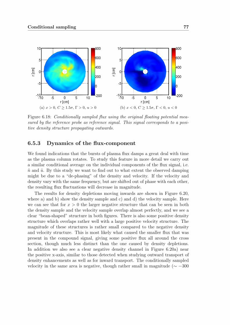
Conditional sampling 77
(a) x > 0, C ≥ 1.5σ, Γ > 0, u > 0 (b) x < 0, C ≥ 1.5σ, Γ < 0, u < 0
Figure 6.18: Conditionally sampled flux using the original floating potential mea-sured by the reference probe as reference signal. This signal corresponds to a posi-tive density structure propagating outwards.
6.5.3 Dynamics of the flux-component
We found indications that the bursts of plasma flux damps a great deal with timeas the plasma column rotates. To study this feature in more detail we carry outa similar conditional average on the individual components of the flux signal, i.e.n and u. By this study we want to find out to what extent the observed dampingmight be due to a “de-phasing” of the density and velocity. If the velocity anddensity vary with the same frequency, but are shifted out of phase with each other,the resulting flux fluctuations will decrease in magnitude.
The results for density depletions moving inwards are shown in Figure 6.20,where a) and b) show the density sample and c) and d) the velocity sample. Herewe can see that for x > 0 the larger negative structure that can be seen in boththe density sample and the velocity sample overlap almost perfectly, and we see aclear “bean-shaped” structure in both figures. There is also some positive densitystructure which overlaps rather well with a large positive velocity structure. Themagnitude of these structures is rather small compared to the negative densityand velocity structure. This is most likely what caused the smaller flux that waspresent in the compound signal, giving some positive flux all around the crosssection, though much less distinct than the one caused by density depletions.In addition we also see a clear negative density channel in Figure 6.20a) nearthe positive x-axis, similar to those detected when studying outward transport ofdensity enhancements as well as for inward transport. The conditionally sampledvelocity in the same area is negative, though rather small in magnitude (∼ −300
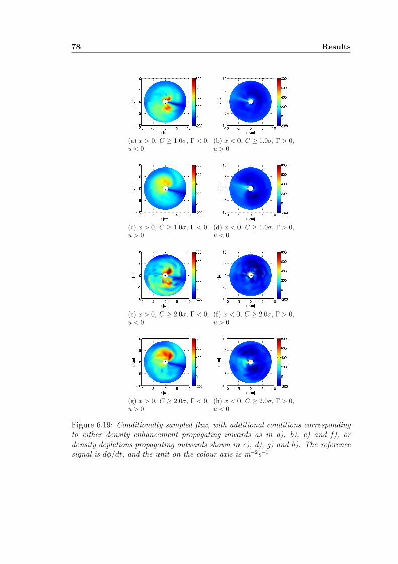
78 Results
(a) x > 0, C ≥ 1.0σ, Γ < 0,u < 0
(b) x < 0, C ≥ 1.0σ, Γ > 0,u > 0
(c) x > 0, C ≥ 1.0σ, Γ < 0,u > 0
(d) x < 0, C ≥ 1.0σ, Γ > 0,u < 0
(e) x > 0, C ≥ 2.0σ, Γ < 0,u < 0
(f) x < 0, C ≥ 2.0σ, Γ > 0,u > 0
(g) x > 0, C ≥ 2.0σ, Γ < 0,u > 0
(h) x < 0, C ≥ 2.0σ, Γ > 0,u < 0
Figure 6.19: Conditionally sampled flux, with additional conditions correspondingto either density enhancement propagating inwards as in a), b), e) and f), ordensity depletions propagating outwards shown in c), d), g) and h). The referencesignal is dφ/dt, and the unit on the colour axis is m−2s−1
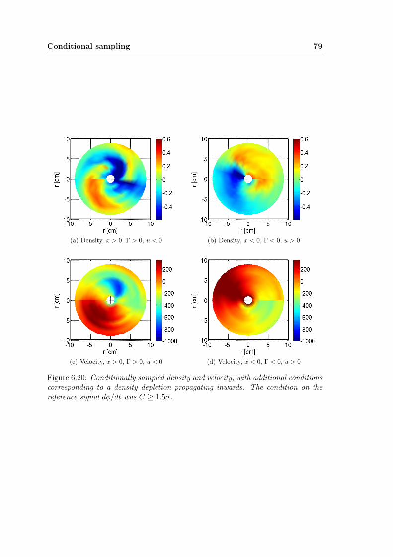
Conditional sampling 79
(a) Density, x > 0, Γ > 0, u < 0 (b) Density, x < 0, Γ < 0, u > 0
(c) Velocity, x > 0, Γ > 0, u < 0 (d) Velocity, x < 0, Γ < 0, u > 0
Figure 6.20: Conditionally sampled density and velocity, with additional conditionscorresponding to a density depletion propagating inwards. The condition on thereference signal dφ/dt was C ≥ 1.5σ.
80 Results
m/s).However, as one moves half a revolution to the negative positions, i.e. x < 0,
we see that the density depletion we saw in a) has reduced in magnitude by afactor ∼ 2. However, the negative channel that originally was near the positive x-axis, has moved around the cross section to the negative x-axis, and is still nearlyequal in magnitude. The positive density structure has mostly maintained its size,though there has been some expansion causing a slight reduction in magnitude. Inthe velocity sample for x < 0 we see that the original negative velocity structurewhich for these positions would be a corresponding positive structure has movedsomewhat further around the cross section. Near the negative y-axis, where wewould now expect to find the coherent structure that is so clear and large inmagnitude for x > 0, we have very small velocities, and the resultant flux willthen be greatly reduced, as we see in Figure 6.13h). However, we have significantvelocities in the area where the narrow density channel is now found. Hence thisstructure is what we do see in the compound signal for x < 0 and correspondingconditions. The velocity maximum has been reduced by a factor ∼ 2 during halfa revolution.
Hence it seems like much of the reason for the damping of the flux signal isthat the velocity and the density develop at different rates, causing them to de-phase. This de-phasing changes which flux structure is most evident as the plasmacolumn rotates.
6.5.4 Conditional variance
As mentioned in Chapter 5 conditional variance as defined by (5.18) is a measureof reproducibility of a signal. For low values of Vcon we have high reproducibilityand for high values of Vcon reproducibility is low. However, it is more intuitive tointerpret a plot of Crep = 1−Vcon, as high values correspond to high reproducibility.Figure 6.21 shows this for a given set of conditions. We consider this one figure tobe representative for all the different combinations of conditions.
Here we see that there is a fairly high level of reproducibility for the areas inwhich we find the coherent flux structures. This is the case for both the largerounded structure near the positive y-axis, but also for the narrow channel thatwe have seen in several figures previously, but which is not that prominent forthese particular conditions (C ≥ 1.5σ, F > 0 and u < 0). This indicates that eventhough this flow channel is very faint in our conditionally sampled average, it isclearly a significant part of the signal. Anywhere else in the cross section Crep isnearly 0, indicating that these sections are too unpredictable. The highest level ofreproducibility found is ∼ 0.6.
Having Crep = 1 is very unlikely as it means that we can reproduce our resultsperfectly.
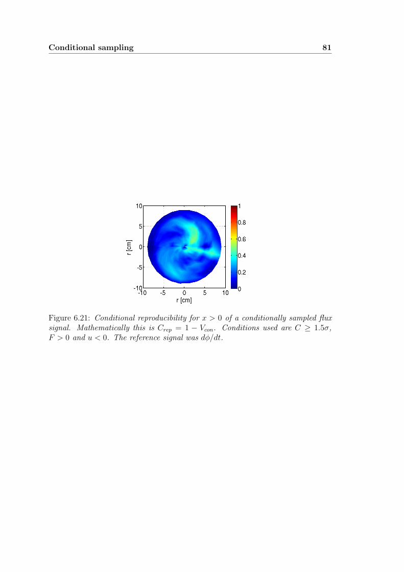
Conditional sampling 81
Figure 6.21: Conditional reproducibility for x > 0 of a conditionally sampled fluxsignal. Mathematically this is Crep = 1 − Vcon. Conditions used are C ≥ 1.5σ,F > 0 and u < 0. The reference signal was dφ/dt.

82 Results
Chapter 7
Discussion and conclusion
In this chapter the results presented in Chapter 6 are discussed and interpreted,attempting to explain what our results mean. The discussion is linked to thedifferent forms of turbulent transport outlined previously. The results are thensummarised and some suggestions for future work are outlined. Note that thedriving mechanism for the turbulent transport will not be addressed.
7.1 Statistical properties
The statistical properties of the data offer much insight into the average motionwe see in the plasma, and are thus useful in studying the motion of the turbulentpart of the plasma column as a whole. Single flux bursts are less prominent in thispart of the analysis and will be discussed later.
7.1.1 General properties of the plasma fluctuations
Looking at the PDFs of velocity, density and flux it appears as though we havelarger values for all variables on the low-field side. The distributions are morepeaked for x < 0, indicating smaller flux events, corresponding with the expectedlower velocities and density perturbations. It is important to keep in mind thatour configuration is toroidal, and thus not symmetric around a toroidal axis. Theideal case would be to have an infinitely long cylindrical tank. However, this isimpossible in the real world, although many Q-machine experiments (Motley, 1975)operate with long magnetised plasma columns. When using such experimentaldevices one has to deal with the additional effects caused by plasma reaching theend of the tank. The other realistic option is to use a torus, where there is no end,but where the magnetic field is curved. However, in a torus there is a significantdifference between the inner side of the tank and the outer side. When the plasma
84 Discussion and conclusion
column rotates around the toroidal axis, moving from the low-field side to thehigh-field side, the plasma must be compressed due to conservation of mass. Thisis because the circumference is greater on the low field side than on the high fieldside, so the same amount of plasma needs to be denser in order to occupy the samearea in the poloidal cross section, while being compressed in the toroidal direction.
The largest fluctuations are found near the centre of the cross section. Theplasma source is located near here, and thus there is more turbulence in this area.In addition, the motion seems to be less coherent with respect to the motion ofplasma located further away from the source. The plasma discharge at the filamentcauses much disturbance, and thus there is little sign of coherence here. The largerstructures are mostly detectable for positions |x| ≥ 2cm.
The joint PDFs of velocity and density demonstrate that there is a correlationbetween the sign of these to physical quantities, and that this correlation changeswhen moving from negative positions to positive. For x > 0 the correlation ispositive, i.e. positive velocity tends to indicate positive density as well and viceversa, whereas for x < 0 it is negative. Clearly large positive flux events arefavoured for x > 0, and here the largest flux events tend to be caused by plasmadepletions moving inwards, though the most frequent events are plasma blobsmoving outwards. The further away from the centre the probes are positioned, thesmaller the fluctuations appear to be, and thus the joint PDF is also more limited.
7.1.2 Skewness kurtosis relations
The investigation of a possible relation between skewness and kurtosis for the fluxsignal gave excellent results. A clear parabolic connection can be seen similar towhat was found by Labit et al. (2007), although they analysed a different signal.Not only was it evident for the particular data from this experiment, but it couldalso be seen for the data sampled from an argon plasma experiment, also conductedusing Blaamann. However, the parabola resulting from the latter data appearedto have different coefficients A and B. This indicates that the general relationK = AS 2 + B may well be a general property of the fluctuations in a plasmacolumn, though that it would likely be useful to treat the different types of plasmaseparately.
It has previously been demonstrated that smoke columns appear to have thischaracteristic relation between skewness and kurtosis too (Jørgensen et al., 2010).They also found a relation between skewness and normalised variance, that we wereunable to reproduce here. Given the electromagnetic nature of plasma fluctuations,it is interesting to see that at least the characteristic relation between skewnessand kurtosis can be detected in plasma as well as in a neutral gas.
Coherent structures 85
7.2 Coherent structures
From both the cross correlation functions and the conditional sampling and av-eraging it seems evident that we have coherent structures in the plasma. Thesestructures appear to be moving around the poloidal cross section along with theclock-wise E×B/B2-velocity of the background plasma, as well as moving in theradial direction. The size of these structures are ∼ 4cm across and ∼ 7 cm inlength. The structure appears to be elongated in the radial direction, as well assomewhat distorted by the circular motion, giving it a bean-like shape. The dis-tribution within the structure indicates a slightly steeper edge in front than inthe back, but there is little sign of the typical mushroom-shape associated withplasma blobs. The poloidal background angular velocity is fairly similar in magni-tude throughout the entire plasma column, which means the background plasmarotates almost like a rigid body. The coherent structure is transported aroundwith the background plasma, but at the same time it is propagating outwards inthe radial direction, getting distorted and eventually dissolving. Typically, onesuch structure will propagate around the poloidal cross section in 100µs, given theperiod of the oscillations in the cross correlation function between the flux andthe reference probe. The coherent nature of the structure is maintained for ∼ 1revolution.
When we were investigating positive bursts of flux we found more events whenlooking for enhancements moving outwards than depletions moving inwards. How-ever, the amplitude of the averaged events were larger for u < 0. This indicatesthat the largest flux events are caused by holes moving inwards rather than en-hancements moving outwards, but that enhancements moving inwards are morecommon. This is consistent with the joint probability distribution of the velocityand flux shown in Figures 6.4 and 6.5. For positive positions the tail stretchingtowards negative u and n is longer and reaches greater numerical values for u,than the corresponding positive tail, while the peak of the distribution is slightlyshifted towards combinations of positive density and velocity.
The coherent structures are mainly detected on the outer side of the torus, i.e.the low B-field side. On this side the curvature and ∇B-drifts contribute to themotion of the electrons, while slowing ions down. On the high B-field side, wehave to opposite case, with electrons in the bulk plasma being slowed down bythe drifts due to inhomogeneities in the magnetic field. Some of the reason forwhy we mainly see coherent structures for x > 0 is that the correlation betweenthe reference signal and the data from the moveable probe is greatly reduced afterthree quarters of a revolution. For x > 0 the plasma has only moved a quarter ofa revolution, and therefore we have better correlation, and more evident coherentstructures are found. When conditionally sampling data from x < 0 it is likely thatsome of the larger events are not sampled, simply because they are not moving
86 Discussion and conclusion
with the exact same speed as the background plasma, and are therefore not withinthe conditionally sampled time intervals.
The flux structures are observed to be damped rather quickly, and appear tomove approximately one revolution before dissolving. However, the flux correlationsignal has a longer correlation period, and thus it appears as though the flux signalis not merely damped by a reduction of u and n, but is reduced because the velocityand density fluctuations move out of phase, hence reducing the resulting flux signal.Whether this is due to a global difference in phase throughout the whole signal,or if it is caused by small phase differences within single events is difficult to say.In order to investigate this one would have to look more closely on each event, butlimited time prevented me from doing so here.
It is important to remember that the resulting coherent structure found usingconditional sampling may differ a great deal from the individual structures. Seeingas the resulting conditional average based on few events shows a much more turbu-lent picture, with smaller structures appearing in a addition to the structure seenin corresponding plots based on more events, it appears as though the structuresin the flux signal constitute a variety of shapes.
It has been shown previously that the conditional averaging technique has atendency to give too small amplitudes for the coherent structures (Teliban et al.,2007). As we can see on our data as well, the amplitude of the coherent structuresappear to increase with increasing trigger level, i.e. the condition C, indicatingthat we are including events which cause a damping of the amplitude. This ten-dency can be dealt with by computing the correlation between the selected events,and removing those which cause this amplitude damping. However, one of the ad-vantages of the conditional sampling technique is that it is easy to implement andinterpret, thus we have kept it in its simple form, and adding additional conditionson the other signals to improve it instead.
7.3 Anomalous transport
The turbulence we see in these data is characterised by a broad spectrum, with afew narrow spikes in the power spectra. Given that we see evidence of coherentstructures in the conditional averages, it is evident that we have bursts and har-monic oscillations which are phase correlated. If they were not, they would havebeen eliminated through the averaging, rather than emphasised.
The transport we see here appears to be consistent with turbulent transport,though it is quite clear that we are looking at events within the ballistic limit. Theballistic motion is mediated by a coherent plasma flow-channel having a looselywound spiral form. Our structures maintain their shape for about one revolution,and are transported around in the azimuthal direction with a rotation frequency
Anomalous transport 87
of ∼ 10 kHz. Hence we are dealing with short timescales. The structures thatwe detect are elongated and seem consistent with the early time evolution of astructure whose motion is dominated by turbulent diffusion (see Figure 3.1). Nodiffusion limit is found. This is consistent with the findings of Fattorini et al.(2012).
Despite the fact that previous studies have shown indication of blob motionalso in experiments similar to the Blaamann plasma (D’Ippolito et al., 2011), inthese data there does not seem to be much proof of it. Even though we havepositively skewed density distribution for the outer positions, the correspondingkurtosis is very close to the Gaussian value. There is also little evidence in thedata of structures exhibiting the characteristic shape associated with blobs.
7.3.1 Vortex structures
An interesting discovery was the presence of a negative flow channel that wasvisible for both positive and negative probe positions. This channel is limited inwidth, but is clearly extended outwards from the very centre of the cross sectionto the more extreme positions. Considering our background material we would ingeneral only expect transport out of the plasma, and as we have seen, of a burst-like nature. However, inward transport of plasma may be an indication that thisparticular structure is part of a compound structure that is more complex than amere flow channel.
Combined with the fact that we find this channel of inward transport in com-bination with outward transport elsewhere in the cross section indicates that wemay have large scale vortex structures here. They are harder to identify as we donot have data from the entire cross section, but only along a string along the localx-axis. It is also important to keep in mind that when conducting the conditionalsampling with the additional conditions, it is only the midpoint of each intervalthat has to satisfy the conditions. We have no guarantee that the structures we seeanywhere else in the cross section follow the same criteria. Thus even though wedemand that the mid point only samples events corresponding to density enhance-ments moving outwards, any structure that is not situated near the middle of thetime interval in which data has been conditionally sampled, but still exhibiting apositive flux may in fact be a density depletion moving inwards. We have no wayof separating the two from each other since they are equivalent when it comes totransport of plasma.
When looking at the conditionally sampled velocity shown in Figure 6.21 we seethat velocity tends to be positive on one side of the cross section and negative on theopposite side. This indicates that we have structures moving inwards on one side,and moving outwards on the opposite side, consistent with a vortex transportingplasma around in large circles, while also being transported clockwise around the
88 Discussion and conclusion
cross section by the background E × B-drift. Plasma propagating outwards willthen be caught in such a vortex, which then drags the plasma back towards thecentre of the column, giving this channel of local negative flux. Whether theconfiguration consists of one or two vortices is difficult to say for certain. Bothcases have been identified in previous studies.
Vortices or vortex-like structures in the Blaamann plasma is consistent withother experiments conducted using Blaamann, such as Øynes et al. (1998); Fredrik-sen et al. (2003b). Interestingly enough it is also consistent with the results of Huldet al. (1991), in which a cylindrical plasma device was used.
7.4 Summary
The aim of this study has been to study the flux of plasma in a simple magnetisedtorus with no rotational transform. The transport has been studied using varioustechniques, including studying probability distributions, correlation and use ofconditional sampling.
The distribution of the flux was compared to a theoretical model deducedby Carreras et al. (1996). We found that our experimental data are similarlydistributed, though the details of the theoretical distribution give less accurateresults, as it is an oversimplification of our case. Assuming Gaussian distributedvelocity and density becomes too great a simplification to give excellent results. Itis also interesting to notice that even though the theoretical model is a universalmodel that ought to be applicable to all kinds of plasma, we found that in termsof skewness and kurtosis it was not appropriate as a model for argon plasma.
Our study of the turbulent flows within the toroidal Blaamann plasma hasrevealed coherent structures propagating around with the background plasma, butalso transporting plasma out towards the wall of the tank, following spiral orbits.These structures appear in nature to be burst-like, i.e. within the short timescalesof turbulent diffusion, and show little indication of being blob-like.
Statistically the average flow is out of the plasma, as is expected given themagnetic configuration of this experiment. We see this also from the estimatedaverage of the flux in each position. However, we have some inward transport inaddition, which leads us to believe that we have large scale vortices or vortex-likestructures in the plasma. These cause plasma to be transported around in smallercircles, while at the same time propagating around the poloidal cross section alongwith the background plasma.

Future perspectives 89
7.5 Future perspectives
As there is a limited amount of time one is allowed to spend on a Master thesis,there are a number of goals and ideas that could not be realised in time. However,should the opportunity appear, the ideas believed to be most interesting are listedhere. If we should get a chance to continue this study we could look into thefollowing:
Investigate intermittency in more detail.
Implement a matched filter, either by searching for a pre-chosen signal shape,or by investigating the curvature of the individual bursts and comparing themfor each set and probe position.
Further investigation of skewness/kurtosis relation could prove interesting.One possibility is to look into the relation for density or velocity fluctuationsindividually, rather than the combined flux signal.
Comparing with synthetic data, by simulating a two-dimensional image ofthe transport that we see, with similar distribution of density and velocity.
Compare with data from other devices, both simple magnetised tori andtokamaks.
Conduct a similar investigation of the available argon data, where partshave been analysed already in the present study when discussing a possibleuniversal relation between skewness and kurtosis.
Out of curiosity one might investigate the conditionally sampled signal fornegative spikes, though we would expect the results to be similar to thosewe have already found for positive spikes.

90 Discussion and conclusion

Appendix A
Source code
Here we include all the Matlab code used to analyse the Blaamann data numer-ically. All code is based on the methods described in Chapter 5, and is includedhere to show numerically how it was all implemented. As the programs all arerather short and simple, there is not a separate chapter about them in the thesis.The code is thoroughly commented in order to explain what is the function ofeach step in every program. In some cases Matlab already had a function thatcalculated a particular quantity we were interested in. In such cases the Matlabfunction was used, as that tended to give the most efficient programs.
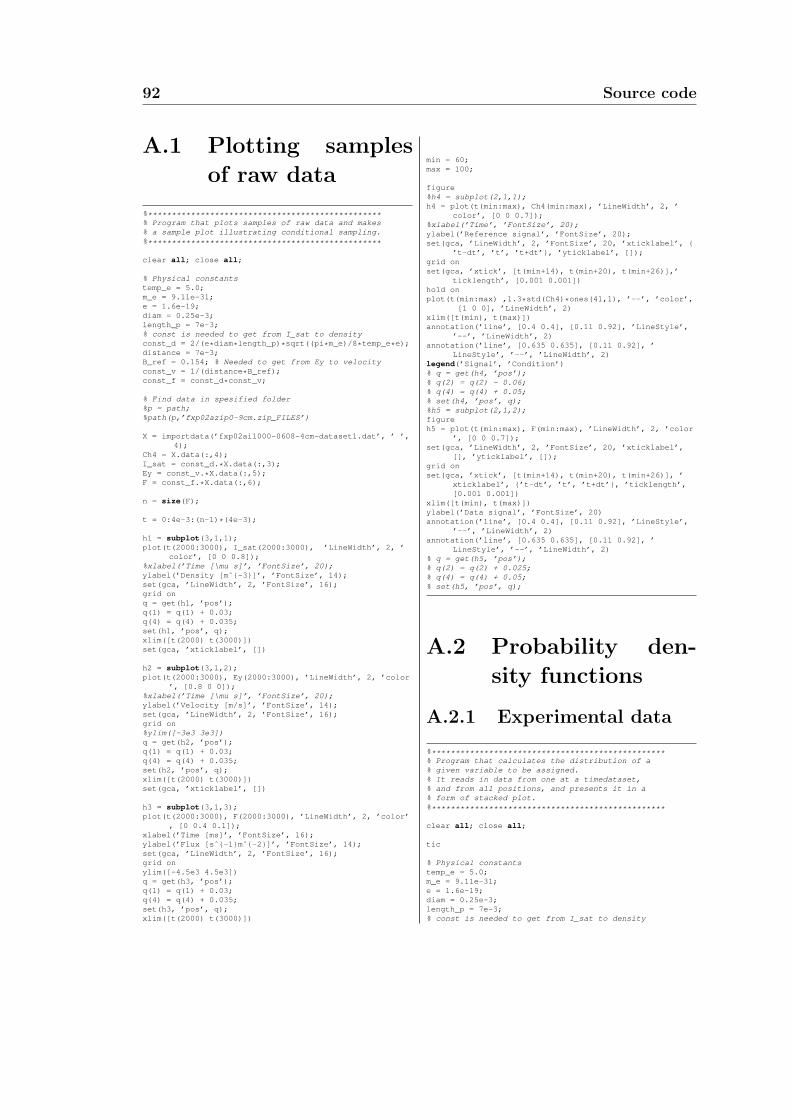
92 Source code
A.1 Plotting samples
of raw data
%*************************************************% Program that plots samples of raw data and makes% a sample plot illustrating conditional sampling.%*************************************************
clear all; close all;
% Physical constantstemp_e = 5.0;m_e = 9.11e-31;e = 1.6e-19;diam = 0.25e-3;length_p = 7e-3;% const is needed to get from I_sat to densityconst_d = 2/(e*diam*length_p)*sqrt((pi*m_e)/8*temp_e*e);distance = 7e-3;B_ref = 0.154; % Needed to get from Ey to velocityconst_v = 1/(distance*B_ref);const_f = const_d*const_v;
% Find data in spesified folder%p = path;%path(p,’fxp02azip0-9cm.zip_FILES’)
X = importdata(’fxp02ai1000-0608-4cm-dataset1.dat’, ’ ’,4);
Ch4 = X.data(:,4);I_sat = const_d.*X.data(:,3);Ey = const_v.*X.data(:,5);F = const_f.*X.data(:,6);
n = size(F);
t = 0:4e-3:(n-1)*(4e-3);
h1 = subplot(3,1,1);plot(t(2000:3000), I_sat(2000:3000), ’LineWidth’, 2, ’
color’, [0 0 0.8]);%xlabel(’Time [\mu s]’, ’FontSize’, 20);ylabel(’Density [mˆ-3]’, ’FontSize’, 14);set(gca, ’LineWidth’, 2, ’FontSize’, 16);grid onq = get(h1, ’pos’);q(1) = q(1) + 0.03;q(4) = q(4) + 0.035;set(h1, ’pos’, q);xlim([t(2000) t(3000)])set(gca, ’xticklabel’, [])
h2 = subplot(3,1,2);plot(t(2000:3000), Ey(2000:3000), ’LineWidth’, 2, ’color
’, [0.8 0 0]);%xlabel(’Time [\mu s]’, ’FontSize’, 20);ylabel(’Velocity [m/s]’, ’FontSize’, 14);set(gca, ’LineWidth’, 2, ’FontSize’, 16);grid on%ylim([-3e3 3e3])q = get(h2, ’pos’);q(1) = q(1) + 0.03;q(4) = q(4) + 0.035;set(h2, ’pos’, q);xlim([t(2000) t(3000)])set(gca, ’xticklabel’, [])
h3 = subplot(3,1,3);plot(t(2000:3000), F(2000:3000), ’LineWidth’, 2, ’color’
, [0 0.4 0.1]);xlabel(’Time [ms]’, ’FontSize’, 16);ylabel(’Flux [sˆ-1mˆ-2]’, ’FontSize’, 14);set(gca, ’LineWidth’, 2, ’FontSize’, 16);grid onylim([-4.5e3 4.5e3])q = get(h3, ’pos’);q(1) = q(1) + 0.03;q(4) = q(4) + 0.035;set(h3, ’pos’, q);xlim([t(2000) t(3000)])
min = 60;max = 100;
figure%h4 = subplot(2,1,1);h4 = plot(t(min:max), Ch4(min:max), ’LineWidth’, 2, ’
color’, [0 0 0.7]);%xlabel(’Time’, ’FontSize’, 20);ylabel(’Reference signal’, ’FontSize’, 20);set(gca, ’LineWidth’, 2, ’FontSize’, 20, ’xticklabel’,
’t-dt’, ’t’, ’t+dt’, ’yticklabel’, []);grid onset(gca, ’xtick’, [t(min+14), t(min+20), t(min+26)],’
ticklength’, [0.001 0.001])hold onplot(t(min:max) ,1.3*std(Ch4)*ones(41,1), ’--’, ’color’,
[1 0 0], ’LineWidth’, 2)xlim([t(min), t(max)])annotation(’line’, [0.4 0.4], [0.11 0.92], ’LineStyle’,
’--’, ’LineWidth’, 2)annotation(’line’, [0.635 0.635], [0.11 0.92], ’
LineStyle’, ’--’, ’LineWidth’, 2)legend(’Signal’, ’Condition’)% q = get(h4, ’pos’);% q(2) = q(2) - 0.06;% q(4) = q(4) + 0.05;% set(h4, ’pos’, q);%h5 = subplot(2,1,2);figureh5 = plot(t(min:max), F(min:max), ’LineWidth’, 2, ’color
’, [0 0 0.7]);set(gca, ’LineWidth’, 2, ’FontSize’, 20, ’xticklabel’,
[], ’yticklabel’, []);grid onset(gca, ’xtick’, [t(min+14), t(min+20), t(min+26)], ’
xticklabel’, ’t-dt’, ’t’, ’t+dt’, ’ticklength’,[0.001 0.001])
xlim([t(min), t(max)])ylabel(’Data signal’, ’FontSize’, 20)annotation(’line’, [0.4 0.4], [0.11 0.92], ’LineStyle’,
’--’, ’LineWidth’, 2)annotation(’line’, [0.635 0.635], [0.11 0.92], ’
LineStyle’, ’--’, ’LineWidth’, 2)% q = get(h5, ’pos’);% q(2) = q(2) + 0.025;% q(4) = q(4) + 0.05;% set(h5, ’pos’, q);
A.2 Probability den-
sity functions
A.2.1 Experimental data
%*************************************************% Program that calculates the distribution of a% given variable to be assigned.% It reads in data from one at a timedataset,% and from all positions, and presents it in a% form of stacked plot.%*************************************************
clear all; close all;
tic
% Physical constantstemp_e = 5.0;m_e = 9.11e-31;e = 1.6e-19;diam = 0.25e-3;length_p = 7e-3;% const is needed to get from I_sat to density
Source code 93
const_d = 2/(e*diam*length_p)*sqrt((pi*m_e)/8*temp_e*e);distance = 7e-3;B_ref = 0.154; % Needed to get from Ey to velocityconst_v = 1/(distance*B_ref);const_f = const_d*const_v;
% Number of intervals in histogramn = 201;V_edges = linspace(-200, 200, n);binwidth = abs(V_edges(2)-V_edges(1));f_k = zeros(n, 19);
N = 10000; % Number of datapoints
for l=-9:1:9
% Assigns the right folder for data% from the corresponding positionif l<0
p = path;path(p, ’fxp02azip-1--9cm.zip_FILES’)
elsep = path;path(p, ’fxp02azip0-9cm.zip_FILES’)
end
% Excludes dataset 5 for position -1cm and 0cm,% as they are missing. Set 4 for -1cm is% removed due to error.if l==-1
S = 3;elseif l==0
S = 4;else
S = 5;end
Ch1 = zeros(N*S, 1);Ch2 = zeros(N*S, 1);I_sat = zeros(N*S, 1);Ch4 = zeros(N*S, 1);Ey = zeros(N*S, 1);F = zeros(N*S, 1);
% Read in datafor i=1:S
X(i) = importdata(sprintf(’fxp02ai1000-0608-%dcm-dataset%d.dat’, l, i), ’ ’, 4);
Ch1((i-1)*N+1:N*i) = X(i).data(:, 1);Ch2((i-1)*N+1:N*i) = X(i).data(:, 2);I_sat((i-1)*N+1:N*i) = X(i).data(:, 3);Ch4((i-1)*N+1:N*i) = X(i).data(:, 4);Ey((i-1)*N+1:N*i) = X(i).data(:, 5);F((i-1)*N+1:N*i) = X(i).data(:, 6);
end
% Assign variablev1 = const_f*F;y1 = ’Flux’;
% Generates values along x-axisdt = 4e-6;t = linspace(0, dt*(N-1), N);
% Sorts data in ascending orderV = sort(v1, 1);
%f = zeros(n, 1);
f_k(:,l+10) = ksdensity(V(:), V_edges, ’function’, ’pdf’);
%f_k(:,l+10) = (histc(v1(:), V_edges))/(S*N*binwidth);
end
y = -9:1:9;
figureh2 = surf(V_edges, y, f_k’);set(h2, ’LineWidth’, 2.5, ’EdgeColor’, ’interp’, ’
FaceColor’, ’none’, ’MeshStyle’, ’Row’)shading flatcolormap jet
%colorbar(’location’, ’EastOutside’);%caxis([0 30]);hidden offtitle(sprintf(’%s distribution’, y1), ’FontSize’, 20)grid onset(gca,’FontSize’,20, ’LineWidth’, 2)xlabel(sprintf(’%s [mˆ-2sˆ-1]’, y1), ’FontSize’, 20)
;ylabel(’Position [cm]’, ’FontSize’, 20);zlabel(’Relative Frequency’, ’FontSize’, 20);xlim([min(V_edges) max(V_edges)])ylim([-9.1 9.1])zlim([0 max(max(f_k))])view([10 30 35]);%saveas(h2,sprintf(’pdf%s.eps’, y1), ’psc2’)
toc
A.2.2 Theoretical model
%*************************************************% Program that calculates the theoretical% distribution of a the flux signal% for all positions, and presents it in a% form of stacked plot.%*************************************************
clear all; close all;
tic
% Physical constantstemp_e = 5.0;m_e = 9.11e-31;e = 1.6e-19;diam = 0.25e-3;length_p = 7e-3;% const is needed to get from I_sat to densityconst_d = 2/(e*diam*length_p)*sqrt((pi*m_e)/8*temp_e*e);distance = 7e-3;B_ref = 0.154; % Needed to get from Ey to velocityconst_v = 1/(distance*B_ref);const_f = const_d*const_v;
% Number of intervals in histogramn = 1601;V_edges = linspace(-200, 200, n);binwidth = abs(V_edges(2)-V_edges(1));
N = 10000; % Number of datapoints
f_k = zeros(n, 19);
%gamma = 0.85;
smooth_param = [45 45 45 45 45 45 65 65 275 301 301 275205 185 115 105 55 55 55];
for l=-9:1:9
% Assigns the right folder for data% from the corresponding positionif l<0
p = path;path(p, ’fxp02azip-1--9cm.zip_FILES’)
elsep = path;path(p, ’fxp02azip0-9cm.zip_FILES’)
end
% Excludes dataset 5 for position -1cm and 0cm,% as they are missing. Set 4 for -1cm is% removed due to error.if l==-1
S = 3;elseif l==0
S = 4;else
94 Source code
S = 5;end
Ch1 = zeros(N*S, 1);Ch2 = zeros(N*S, 1);I_sat = zeros(N*S, 1);Ch4 = zeros(N*S, 1);Ey = zeros(N*S, 1);F = zeros(N*S, 1);
% Read in datafor i=1:S
X(i) = importdata(sprintf(’fxp02ai1000-0608-%dcm-dataset%d.dat’, l, i), ’ ’, 4);
Ch1((i-1)*N+1:N*i) = X(i).data(:, 1);Ch2((i-1)*N+1:N*i) = X(i).data(:, 2);I_sat((i-1)*N+1:N*i) = X(i).data(:, 3);Ch4((i-1)*N+1:N*i) = X(i).data(:, 4);Ey((i-1)*N+1:N*i) = X(i).data(:, 5);F((i-1)*N+1:N*i) = X(i).data(:, 6);
end
% Assign variablev1 = const_f*F;y1 = ’Flux’;
sigma_n = std(const_d*I_sat);sigma_v = std(const_v*Ey);
gamma = corrcoef(const_d*I_sat, const_v*Ey);
% Generates values along x-axisdt = 4e-6;t = linspace(0, dt*(N-1), N);
p = (1/pi)*((sqrt(1-gamma(1,2)ˆ2))/(sigma_n*sigma_v))*besselk(0, abs(V_edges(:))./(sigma_n*sigma_v)).*exp(-gamma(1,2)*V_edges(:)./(sigma_n*sigma_v));
% Sorts data in ascending order%V = sort(v1, 1);p((n-1)/2+1) = (p((n-1)/2)+p((n-1)/2+2))/2+(p((n-1)
/2)-p((n-1)/2-1));
mean(p)
%f_k(1:9*(n-1)/20,l+10) = smooth(p(1:9*(n-1)/20),175);
%f_k(11*(n-1)/20:n,l+10) = smooth(p(11*(n-1)/20:n),175);
%f_k(9*(n-1)/20+1:11*(n-1)/20-1,l+10) = smooth(p(9*(n-1)/20+1:11*(n-1)/20-1), smooth_param(l+10));
f_k(:, l+10) = smooth(p, smooth_param(l+10));end
y = -9:1:9;
figureh = surf(V_edges, y, f_k’);set(h, ’LineWidth’, 2.5, ’EdgeColor’, ’interp’, ’
FaceColor’, ’none’, ’MeshStyle’, ’Row’)shading flatcolormap jet%colorbar(’location’, ’EastOutside’);%caxis([0 30]);hidden offtitle(sprintf(’%s distribution’, y1), ’FontSize’, 20)grid onset(gca,’FontSize’,20, ’LineWidth’, 2)xlabel(sprintf(’%s [mˆ-2sˆ-1]’, y1), ’FontSize’, 20)
;ylabel(’Position [cm]’, ’FontSize’, 20);zlabel(’Relative Frequency’, ’FontSize’, 20);xlim([min(V_edges) max(V_edges)])ylim([-9.1 9.1])zlim([0 max(max(f_k))])view([10 30 35]);
toc
A.2.3 Joint PDF
%*************************************************% Program that calculates the joint PDF of v_x and% density. This is done directly from the dataset% by looking at v_x(i) and d(i).%*************************************************
clear all; close all;
tic% Physical constantstemp_e = 5.0;m_e = 9.11e-31;e = 1.6e-19;diam = 0.25e-3;length_p = 7e-3;% const is needed to get from I_sat to densityconst_d = 2/(e*diam*length_p)*sqrt((pi*m_e)/8*temp_e*e);distance = 7e-3;B_ref = 0.154; % Needed to get from Ey to velocityconst_v = 1/(distance*B_ref);const_f = const_d*const_v;
% Number of datapointsN = 10000;
% Number of intervals in histogramnd = 100;nv = 100;
% Creates intervals for histogramD_edges = linspace(-2, 2.5, nd);V_edges = linspace(-2000, 1200, nv);
% Redefines interval vectors to work% better when finding the joint PDFD_edges = [(D_edges) max(D_edges)+(D_edges(2)-D_edges(1)
)];V_edges = [(V_edges) max(V_edges)+(V_edges(2)-V_edges(1)
)];
% Joint PDFJ_dep = zeros(nd,nv);
%empty array for size of distributionsize_dist = zeros(19,1);
for l=1:1:9%J_dep(:,:) = 0;
% Assigns the right folder for data% from the corresponding position
if l<0p = path;path(p, ’fxp02azip-1--9cm.zip_FILES’)
elsep = path;path(p, ’fxp02azip0-9cm.zip_FILES’)
end
% Excludes dataset 5 for position -1cm and 0cm,% as they are missing. Set 4 from -1cm is% removed due to error.if l==-1
S = 3;elseif l==0
S = 4;else
S = 5;end
for q=1:S% Read in data from positions 0-9 cmX(q) = importdata(sprintf(’fxp02ai1000-0608-%dcm
-dataset%d.dat’, l, q), ’ ’, 4);%Ch1(:, q) = X(q).data(:, 1);%Ch2(:, q) = X(q).data(:, 2);D = const_d*X(q).data(:, 3);%Ch4(:, q) = X(q).data(:, 4);V = const_v*X(q).data(:, 5);%F(:, q) = X(q).data(:, 6);
Source code 95
% Calculating joint PDFfor i=1:N
for j=1:length(D_edges)-1for k=1:length(V_edges)-1
if D(i) < D_edges(j+1) && D(i)>=D_edges(j) && V(i)<V_edges(k+1)&& V(i)>= V_edges(k)
J_dep(j, k) = J_dep(j, k) + 1;end
endend
endend
%J_dep = J_dep./(S*N);end
J_dep = J_dep./(N*9*5);
% Plot dependent joint PDFfigureh1 = image(V_edges(1:nv), D_edges(1:nd), J_dep, ’
CDataMapping’, ’Scaled’);shading interp;%set(h1)colormap jet;colorbargrid onxlabel(’Velocity [m/s]’, ’FontSize’, 16)ylabel(’Density [mˆ-3]’, ’FontSize’, 16)caxis([0 13.5e-4])%zlabel(’Relative Frequency’, ’FontSize’, 24)%axis tight%xlim([V_edges(1) V_edges(nv+1)]);%ylim([D_edges(1) D_edges(nd+1)]);%set(gca, ’YDir’, ’reverse’)set(gca, ’LineWidth’, 2, ’FontSize’, 16, ’YDir’, ’normal
’)%title(’Joint PDF’, ’FontSize’, 20)%view([0 0 90])
toc
A.3 Statisitical mo-
ments
A.3.1 All sets treated asone long string ofdata
%*************************************************% Program for investigating the moments of the% timeseries, and plotting them aginst position,% but also againts each other. For each position% the mean of the moment in question is calculated% from the mean of all the datasets.%*************************************************
%clear all; close all;
% Physical constantstemp_e = 5.0;m_e = 9.11e-31;e = 1.6e-19;diam = 0.25e-3;length_p = 7e-3;% const is needed to get from I_sat to densityconst_d = 2/(e*diam*length_p)*sqrt((pi*m_e)/8*temp_e*e);distance = 7e-3;B_ref = 0.154; % Needed to get from Ey to velocity
const_v = 1/(distance*B_ref);const_f = const_d*const_v;
N = 10000; % Number of datapoints
m = zeros(19, 1);va = zeros(19, 1);skew = zeros(19, 1);kurt = zeros(19, 1);
for k=-9:1:9% Assigns the right folder for data from% the corresponding positionif k<0
p = path;path(p, ’fxp02azip-1--9cm.zip_FILES’)
elsep = path;path(p, ’fxp02azip0-9cm.zip_FILES’)
end
% Excludes dataset 5 for positions 0cm and -1cm,% as they is missing, in addition to set 4 for% postion -1cm as it is wrong.if k==-1
S = 3;elseif k==0
S = 4;else
S = 5;end
I_sat = zeros(N*S, 1);Ey = zeros(N*S, 1);F = zeros(N*S, 1);
% Read in data from positions 0-9 cmfor i=1:S
X(i) = importdata(sprintf(’fxp02ai1000-0608-%dcm-dataset%d.dat’, k, i), ’ ’, 4);
I_sat((i-1)*N+1:i*N) = const_d*X(i).data(:, 3);Ey((i-1)*N+1:i*N) = const_v*X(i).data(:, 5);F((i-1)*N+1:i*N) = const_f*X(i).data(:, 6);
end
% Assign variablev1 = F;y1 = ’Flux’;
m(k+10) = mean(v1, 1);va(k+10) = var(v1, 1)/(m(k+10))ˆ2;skew(k+10) = skewness(v1, 1);kurt(k+10) = kurtosis(v1, 1);
end
x = linspace(-9,9,19);%% % Makes ordinary plots of moments vs. position% figure(6)% h1 = plot(x, m, ’ro’);% set(h1, ’MarkerSize’, 10, ’LineWidth’, 2)% grid on% set(gca, ’LineWidth’, 2, ’FontSize’, 20)% xlabel(’Position [cm]’, ’FontSize’, 20)% ylabel(’Mean [arbitrary units]’, ’FontSize’, 20)% hold on% %saveas(h1,sprintf(’meanvspos%s.eps’, y1), ’psc2’)%% figure(8)% h2 = semilogy(x, va, ’ro’);% set(h2, ’MarkerSize’, 10, ’LineWidth’, 2)% grid on% set(gca, ’LineWidth’, 2, ’FontSize’, 20)% xlabel(’Position [cm]’, ’FontSize’, 20)% ylabel(’Variance’, ’FontSize’, 20)% hold on% %ylim([0 100])% %saveas(h2,sprintf(’varvspos%s.eps’, y1), ’psc2’)%% figure(3)% h3 = plot(x, skew, ’ro’);% set(h3, ’MarkerSize’, 10, ’LineWidth’, 2)% grid on
96 Source code
% set(gca, ’LineWidth’, 2, ’FontSize’, 20)% xlabel(’Position [cm]’, ’FontSize’, 20)% ylabel(’Skewness’, ’FontSize’, 20)% hold on% %saveas(h3,sprintf(’skewvspos%s.eps’, y1), ’psc2’)%% figure(4)% h4 = plot(x, kurt, ’ro’);% set(h4, ’MarkerSize’, 10, ’LineWidth’, 2)% grid on% hold on% normline = plot(linspace(-10,10,10), 3*ones(10,1),
’--’);% set(normline, ’LineWidth’, 2)% set(gca, ’LineWidth’, 2, ’FontSize’, 20)% xlabel(’Position [cm]’, ’FontSize’, 20)% ylabel(’Kurtosis’, ’FontSize’, 20)% %ylim([0 25])% %saveas(h4,sprintf(’kurtvspos%s.eps’, y1), ’psc2’)
% % Makes plot of kurtosis vs. skewness squared plussone. Each marker has
% % size and color according to position.% for l=1:9% figure(5)% h5 = plot(kurt(l), skew(l)ˆ2+1, ’ro’);% set(h5, ’MarkerSize’, (-4*(l-11)), ’LineWidth’, 2)% hold on% end%% figure(5)% h7 = plot(kurt, skew.ˆ2+1, ’ro’);% hold on% set(h7, ’MarkerSize’, 10, ’LineWidth’, 2)% grid on% set(gca, ’LineWidth’, 2, ’FontSize’, 20)% xlabel(’Kurtosis’, ’FontSize’, 20)% ylabel(’Skewnessˆ2 + 1’, ’FontSize’, 20, ’FontWeight’,
’Bold’)% xlim([0, 20])% ylim([0, 20])%% x1 = linspace(0, 20, 20);% figure(5)% stipline = plot(x1, x1, ’--’);% set(stipline, ’LineWidth’, 2)% %hold off% %saveas(h8,’kurtvsskewsq.eps’, ’psc2’);
% for l=1:9% figure(5)% h6(l) = plot(kurt(l+10), skew(l+10)ˆ2+1, ’bo’);% set(h6(l), ’MarkerSize’, (4*(l+1)), ’LineWidth’,
2);% end%% legend([h5, h7, h6(1)], ’Negative x-values’, ’x=0’, ’
Positive x-values’, ’Location’, ’NorthWest’)
% % Makes plot of skewness vs. kurtosis. Each marker has% % size and color according to position.% for l=1:9% figure(6)% h8 = plot(skew(l), kurt(l), ’ro’);% set(h8, ’MarkerSize’, (-4*(l-11)), ’LineWidth’, 2)% hold on% end
% figure(1)% h9 = plot(skew, kurt, ’ro’);% set(h9, ’MarkerSize’, 10, ’LineWidth’, 2)% grid on% set(gca, ’LineWidth’, 2, ’FontSize’, 20)% xlabel(’Skewness’, ’FontSize’, 20)% ylabel(’Kurtosis’, ’FontSize’, 20)% hold on%saveas(h9,’skewvskurt.eps’, ’psc2’);
% for l=1:9% figure(6)% h10(l) = plot(skew(l+10), kurt(l+10), ’bo’);% set(h10(l), ’MarkerSize’, 4*(l+1), ’LineWidth’, 2)% hold on
% end%% legend([h8, h9, h10(1)], ’Negative x-values’, ’x=0’, ’
Positive x-values’)
% % Makes plot of kurtosis vs. variance squared plussone. Each marker has
% % size and color according to position.% for l=1:9% figure(7)% h11 = plot(kurt(l), va(l), ’ro’);% set(h11, ’MarkerSize’, (-4*(l-11)), ’LineWidth’,
2)% hold on% end
% figure(7)% h12 = plot(kurt, va, ’ro’);% set(h12, ’MarkerSize’, 10, ’LineWidth’, 2)% grid on% set(gca, ’LineWidth’, 2, ’FontSize’, 20)% ylabel(’Variance/<s>ˆ2’, ’FontSize’, 20)% xlabel(’Kurtosis’, ’FontSize’, 20)% hold on% %saveas(h12,’kurtvsvar.eps’, ’psc2’);
% for l=1:9% figure(7)% h13(l) = plot(kurt(l+10), va(l+10), ’bo’);% set(h13(l), ’MarkerSize’, 4*(l+1), ’LineWidth’, 2)% hold on% end%% legend([h11, h12, h13(1)], ’Negative x-values’, ’x=0’,
’Positive x-values’)
% % Makes plot of skewness vs. variance squared plussone. Each marker has
% % size and color according to position.% for l=1:9% figure(8)% h14 = plot(skew(l), va(l), ’ro’);% set(h14, ’MarkerSize’, (-4*(l-11)), ’LineWidth’,
2)% hold on% end%% figure(8)% h15 = plot(skew(10), va(10), ’go’);% set(h15, ’MarkerSize’, 4, ’LineWidth’, 2)% grid on% set(gca, ’LineWidth’, 2, ’FontSize’, 20)% xlabel(’Skewness’, ’FontSize’, 20)% ylabel(’Variance’, ’FontSize’, 20)%% for l=1:9% figure(8)% h16(l) = plot(skew(l+10), va(l+10), ’bo’);% set(h16(l), ’MarkerSize’, 4*(l+1), ’LineWidth’, 2)% hold on% end%% legend([h14, h15, h16(1)], ’Negative x-values’, ’x=0’,
’Positive x-values’)
figure(2)h = semilogy(abs(skew), va, ’ro’);set(h, ’MarkerSize’, 10, ’LineWidth’, 2)grid onset(gca, ’LineWidth’, 2, ’FontSize’, 20)xlabel(’Skewness’, ’FontSize’, 20)ylabel(’Normalised variance’, ’FontSize’, 20)hold onylim([0 10])xlim([0 4])%saveas(h,’absskewvsvar.eps’, ’psc2’);
Source code 97
A.3.2 All sets treated sepa-rately
%*************************************************% Program for investigating the moments of the% timeseries, and plotting them aginst position,% but also againts each other. For each position the% mean of the moment in question is calculated from% the mean of all the datasets.%*************************************************
%clear all; close all;
N = 10000; % Number of datapoints% Physical constantstemp_e = 5.0;m_e = 9.11e-31;e = 1.6e-19;diam = 0.25e-3;length_p = 7e-3;% const is needed to get from I_sat to densityconst_d = 2/(e*diam*length_p)*sqrt((pi*m_e)/8*temp_e*e);distance = 7e-3;B_ref = 0.154; % Needed to get from Ey to velocityconst_v = 1/(distance*B_ref);const_f = const_d*const_v;
m = zeros(19*5-3, 1);va = zeros(19*5-3, 1);skew = zeros(19*5-3, 1);kurt = zeros(19*5-3, 1);
counter = 0;for k=-9:1:9
% Assigns the right folder for data from thecorresponding position
if k<0p = path;path(p, ’fxp02azip-1--9cm.zip_FILES’)
elsep = path;path(p, ’fxp02azip0-9cm.zip_FILES’)
end
% Excludes dataset 5 and 4 for position -1cm,% and set 5 for 0 cm, as they are missing.% Set 4 for -1cm is also removed due to error.if k==-1
S = 3;elseif k==0
S = 4;else
S = 5;end
I_sat = zeros(N, S);Ey = zeros(N, S);F = zeros(N, S);
% Read in data from positions 0-9 cmfor i=1:S
X(i) = importdata(sprintf(’fxp02ai1000-0608-%dcm-dataset%d.dat’, k, i), ’ ’, 4);
I_sat(:, i) = const_d*X(i).data(:, 3);Ey(:, i) = const_v*X(i).data(:, 5);F(:, i) = const_f*X(i).data(:, 6);
end
% Assign variablev1 = F;y1 = ’Flux’;
Mean = zeros(S, 1);Variance = zeros(S, 1);Skewness = zeros(S, 1);Kurtosis = zeros(S, 1);
for j=1:SMean(j) = mean(v1(:,j));Variance(j) = var(v1(:,j), 1)/(Mean(j)ˆ2);% The 1 indicates that the calculated standard
% deviation devides by n and not n-1.Skewness(j) = skewness(v1(:,j), 1);Kurtosis(j) = kurtosis(v1(:,j), 1);
end
if k==-1 && S==3m(41:43) = Mean;va(41:43) = Variance;skew(41:43) = Skewness;kurt(41:43) = Kurtosis;counter = 1;
elseif k==-1 && S==4m(41:44) = Mean;va(41:44) = Variance;skew(41:44) = Skewness;kurt(41:44) = Kurtosis;
elseif k==0 && counter==1m(44:47) = Mean;va(44:47) = Variance;skew(44:47) = Skewness;kurt(44:47) = Kurtosis;
elseif k==0 && counter==0m(45:48) = Mean;va(45:48) = Variance;skew(45:48) = Skewness;kurt(45:48) = Kurtosis;
elseif k<-1m((k+10)*S-S+1:(k+10)*S) = Mean;va((k+10)*S-S+1:(k+10)*S) = Variance;skew((k+10)*S-S+1:(k+10)*S) = Skewness;kurt((k+10)*S-S+1:(k+10)*S) = Kurtosis;
elseif k>0 && counter==1m((k+10)*S-S-2:(k+10)*S-3) = Mean;va((k+10)*S-S-2:(k+10)*S-3) = Variance;skew((k+10)*S-S-2:(k+10)*S-3) = Skewness;kurt((k+10)*S-S-2:(k+10)*S-3) = Kurtosis;
elsem((k+10)*S-S-1:(k+10)*S-2) = Mean;va((k+10)*S-S-1:(k+10)*S-2) = Variance;skew((k+10)*S-S-1:(k+10)*S-2) = Skewness;kurt((k+10)*S-S-1:(k+10)*S-2) = Kurtosis;
end
end
x1 = linspace(-9,9,19);x2 = [-9 -8 -7 -6 -5 -4 -3 -2 1 2 3 4 5 6 7 8 9];x = sort([x1,x1,x1,x2,x2, 0]);
% % Makes ordinary plots of moments vs. position% figure(6)% h1 = plot(x, m, ’o’);% set(h1, ’MarkerSize’, 7, ’LineWidth’, 2)% grid on% set(gca, ’LineWidth’, 2, ’FontSize’, 20)% xlabel(’Position [cm]’, ’FontSize’, 20)% ylabel(’Mean’, ’FontSize’, 20)% hold on%% figure(8)% h2 = plot(x, va, ’o’);% set(h2, ’MarkerSize’, 7, ’LineWidth’, 2)% grid on% set(gca, ’LineWidth’, 2, ’FontSize’, 20)% xlabel(’Position [cm]’, ’FontSize’, 20)% ylabel(’Variance’, ’FontSize’, 20)% %ylim([0 100])% hold on%% figure(3)% h3 = plot(x, skew, ’o’);% set(h3, ’MarkerSize’, 7, ’LineWidth’, 2)% grid on% set(gca, ’LineWidth’, 2, ’FontSize’, 20)% xlabel(’Position [cm]’, ’FontSize’, 20)% ylabel(’Skewness’, ’FontSize’, 20)% hold on%% figure(4)% h4 = plot(x, kurt, ’o’);% set(h4, ’MarkerSize’, 7, ’LineWidth’, 2)% grid on% set(gca, ’LineWidth’, 2, ’FontSize’, 20)
98 Source code
% xlabel(’Position [cm]’, ’FontSize’, 20)% ylabel(’Kurtosis’, ’FontSize’, 20)% hold on%% % % Makes plot of kurtosis vs. skewness squared pluss
one. Each marker has% % % size and color according to position.% % for l=1:9% % figure(5)% % h5 = plot(kurt(l), skew(l)ˆ2+1, ’ro’);% % set(h5, ’MarkerSize’, (-4*(l-11)), ’LineWidth’,
2)% % hold on% % end%% figure(5)% h7 = plot(kurt, skew.ˆ2+1, ’o’);% hold on% set(h7, ’MarkerSize’, 7, ’LineWidth’, 2)% grid on% set(gca, ’LineWidth’, 2, ’FontSize’, 20)% xlabel(’Kurtosis’, ’FontSize’, 20)% ylabel(’Skewnessˆ2 + 1’, ’FontSize’, 20, ’FontWeight’,
’demi’)% xlim([0, 20])% ylim([0, 20])%% x_lin = linspace(0, 20, 20);% figure(5)% stiplin = plot(x_lin, x_lin, ’--’);% set(stiplin, ’LineWidth’, 2, ’Color’, [0 0 0.4])%% modelFun2 = @(q,x) q(1).*x+q(2);% startingVals2 = [1 1];% coefEsts2 = nlinfit(kurt, skew.ˆ2+1, modelFun2,
startingVals2);% xgrid = linspace(0,20,20);% line(xgrid, modelFun2(coefEsts2, xgrid), ’Color’,[0
0.4 0], ’LineWidth’, 2);% hold off%% % for l=1:9% % figure(5)% % h6(l) = plot(kurt(l+10), skew(l+10)ˆ2+1, ’bo’);% % set(h6(l), ’MarkerSize’, (4*(l+1)), ’LineWidth’,
2);% % end% %% % legend([h5, h7, h6(1)], ’Negative x-values’, ’x=0’,
’Positive x-values’, ’Location’, ’NorthWest’)
% % Makes plot of skewness vs. kurtosis. Each marker has% % size and color according to position.% for l=1:9% figure(6)% h8 = plot(skew(l), kurt(l), ’ro’);% set(h8, ’MarkerSize’, (-4*(l-11)), ’LineWidth’, 2)% hold on% end%% figure(1)% h9 = plot(skew, kurt, ’bo’);% set(h9, ’MarkerSize’, 7, ’LineWidth’, 2)% grid on% set(gca, ’LineWidth’, 2, ’FontSize’, 20)% xlabel(’Skewness’, ’FontSize’, 20)% ylabel(’Kurtosis’, ’FontSize’, 20)% hold on% xlim([-4 4])% ylim([0 30])%% modelFun = @(p,x) p(1).*x.ˆ2+p(2);% startingVals = [1 1];% coefEsts = nlinfit(skew, kurt, modelFun, startingVals)
;% xgrid = linspace(-6,6,100);% line(xgrid, modelFun(coefEsts, xgrid), ’Color’,[0 0.4
0], ’LineWidth’, 2);% %hold off%% figure(1)% terline = plot(xgrid, xgrid.ˆ2+1, ’--’);% set(terline, ’LineWidth’, 2)
% for l=1:9% figure(6)% h10(l) = plot(skew(l+10), kurt(l+10), ’bo’);% set(h10(l), ’MarkerSize’, 4*(l+1), ’LineWidth’, 2)% hold on% end%% legend([h8, h9, h10(1)], ’Negative x-values’, ’x=0’, ’
Positive x-values’)
% % Makes plot of kurtosis vs. variance squared plussone. Each marker has
% % size and color according to position.% for l=1:9% figure(7)% h11 = plot(kurt(l), va(l), ’ro’);% set(h11, ’MarkerSize’, (-4*(l-11)), ’LineWidth’,
2)% hold on% end
% figure(7)% h12 = plot(kurt, va, ’o’);% set(h12, ’MarkerSize’, 7, ’LineWidth’, 2)% grid on% set(gca, ’LineWidth’, 2, ’FontSize’, 20)% ylabel(’Variance’, ’FontSize’, 20)% xlabel(’Kurtosis’, ’FontSize’, 20)% hold on
% for l=1:9% figure(7)% h13(l) = plot(kurt(l+10), va(l+10), ’bo’);% set(h13(l), ’MarkerSize’, 4*(l+1), ’LineWidth’, 2)% hold on% end%% legend([h11, h12, h13(1)], ’Negative x-values’, ’x=0’,
’Positive x-values’)
% % Makes plot of skewness vs. variance squared plussone. Each marker has
% % size and color according to position.% for l=1:9% figure(8)% h14 = plot(skew(l), va(l), ’ro’);% set(h14, ’MarkerSize’, (-4*(l-11)), ’LineWidth’,
2)% hold on% end%% figure(8)% h15 = plot(skew(10), va(10), ’go’);% set(h15, ’MarkerSize’, 4, ’LineWidth’, 2)% grid on% set(gca, ’LineWidth’, 2, ’FontSize’, 20)% xlabel(’Skewness’, ’FontSize’, 20)% ylabel(’Variance’, ’FontSize’, 20)%% for l=1:9% figure(8)% h16(l) = plot(skew(l+10), va(l+10), ’bo’);% set(h16(l), ’MarkerSize’, 4*(l+1), ’LineWidth’, 2)% hold on% end%% legend([h14, h15, h16(1)], ’Negative x-values’, ’x=0’,
’Positive x-values’)
figure(2)h = semilogy(abs(skew), va, ’bo’);set(h, ’MarkerSize’, 7, ’LineWidth’, 2)grid onset(gca, ’LineWidth’, 2, ’FontSize’, 20)xlabel(’Skewness’, ’FontSize’, 20)ylabel(’Normalised variance’, ’FontSize’, 20)hold on
x_lin2 = 0:0.1:3;semilogy(x_lin2, 0.5*(2+x_lin2.ˆ2+x_lin2.*sqrt(4+x_lin2
.ˆ2)), ’--’, ’LineWidth’, 2)ylim([0 30])
Source code 99
xlim([0 3])% hold offhold on
A.3.3 Including the Argonplasma data
%*************************************************% Program that reads in data from the Argon% plasma experiment, and calculates skewness,% variance, mean and kurtosis. Due to some% sets missing, a method that skips these% had to be implemented.%*************************************************
clear all; close all;
% Number of points per setN = 10000;
% Empty array for fluxf = zeros(N, 1);
% Number of datasetsS = 23;
for j=1:6% Empty arrays for skewness and kurtosisvariance = zeros(S, 1);skew = zeros(S, 1);kurt = zeros(S, 1);
p = path;path(p,’arbvarhp’)
for i=1:23if i==12 && j==2
continueend% Read datafid = fopen(sprintf(’arb%d00hp.TXT’, j));if j==2 && i>12
C1 = textscan(fid, ’%f %f %f %f’, ’delimiter’, ’ ’, ’HeaderLines’, (i-1)
*10003-8958);else
C1 = textscan(fid, ’%f %f %f %f’, ’delimiter’, ’ ’, ’HeaderLines’, 42+(i-1)*10003);
endfclose(fid);% Calculate fluxf(:) = -(C11-C12).*C13;% Calculate skewness and kurtosis of fluxvariance(i) = var(f, 1)/(mean(f))ˆ2;skew(i) = skewness(f);kurt(i) = kurtosis(f);
end
% figure(1)% h1 = plot(skew, kurt, ’ko’);% grid on% xlabel(’Skewness’, ’FontSize’, 20)% ylabel(’Kurtosis’, ’FontSize’, 20)% %title(’Skewness-kurtosis relation for flux’, ’
FontSize’, 20)% set(h1, ’LineWidth’, 2, ’MarkerSize’, 7)% set(gca, ’LineWidth’, 2, ’FontSize’, 20)% xlim([-4, 4])% ylim([0, 30])% hold on
figure(2)h3 = semilogy(abs(skew), variance, ’ko’);grid onxlabel(’Skewness’, ’FontSize’, 20)ylabel(’Normalised variance’, ’FontSize’, 20)
%title(’Skewness-variance relation for flux’, ’FontSize’, 20)
set(h3, ’LineWidth’, 2, ’MarkerSize’, 7)set(gca, ’LineWidth’, 2, ’FontSize’, 20)%xlim([-4, 4])%ylim([0, 25])hold on
end
for j=1:6% Empty arrays for skewness and kurtosisvariance = zeros(S, 1);skew = zeros(S, 1);kurt = zeros(S, 1);
p = path;path(p,’arbvarlp’)
if j==4for i=3:23
% Read datafid = fopen(sprintf(’arb%d00lp.TXT’, j));C1 = textscan(fid, ’%f %f %f %f’, ’delimiter
’, ’ ’, ’HeaderLines’, 11048+(i-3)
*10003);fclose(fid);% Calculate fluxf(:) = -(C11-C12).*C13;% Calculate skewness and kurtosis of fluxvariance(i) = var(f)/(mean(f))ˆ2;skew(i) = skewness(f);kurt(i) = kurtosis(f);
endelse
for i=1:23% Read datafid = fopen(sprintf(’arb%d00lp.TXT’, j));C1 = textscan(fid, ’%f %f %f %f’, ’delimiter
’, ’ ’, ’HeaderLines’, 42+(i-1)*10003);fclose(fid);% Calculate fluxf(:) = -(C11-C12).*C13;% Calculate skewness and kurtosis of fluxvariance(i) = var(f)/(mean(f))ˆ2;skew(i) = skewness(f);kurt(i) = kurtosis(f);
endend
% figure(1)% h2 = plot(skew, kurt, ’ko’);% grid on% xlabel(’Skewness’, ’FontSize’, 20)% ylabel(’Kurtosis’, ’FontSize’, 20)% %title(’Skewness-kurtosis relation for flux’, ’
FontSize’, 20)% set(h2, ’LineWidth’, 2, ’MarkerSize’, 7)% set(gca, ’LineWidth’, 2, ’FontSize’, 20)% xlim([-4, 4])% ylim([0, 30])% hold on%
figure(2)h5 = semilogy(abs(skew), variance, ’ko’);grid onxlabel(’Skewness’, ’FontSize’, 20)ylabel(’Normalised variance’, ’FontSize’, 20)%title(’Skewness-variance relation for flux’, ’
FontSize’, 20)set(h5, ’LineWidth’, 2, ’MarkerSize’, 7)set(gca, ’LineWidth’, 2, ’FontSize’, 20)%xlim([-4, 4])%ylim([0, 25])hold on
end
for j=10:5:15% Empty arrays for skewness and kurtosisvariance = zeros(S, 1);skew = zeros(S, 1);kurt = zeros(S, 1);
p = path;
100 Source code
path(p,’arbvarlp’)
for i=1:23if j==15 && i==10
continueend% Read datafid = fopen(sprintf(’arb%d0pla.TXT’, j));if j==15 && i>10
C1 = textscan(fid, ’%f %f %f %f’, ’delimiter’, ’ ’, ’HeaderLines’, (i-1)
*10003-8955);else
C1 = textscan(fid, ’%f %f %f %f’, ’delimiter’, ’ ’, ’HeaderLines’, 45+(i-1)*10003);
endfclose(fid);% Calculate fluxf(:) = -(C11-C12).*C13;% Calculate skewness and kurtosis of fluxvariance(i) = var(f)/(mean(f))ˆ2;skew(i) = skewness(f);kurt(i) = kurtosis(f);
end
% figure(1)% h2 = plot(skew, kurt, ’ko’);% grid on% xlabel(’Skewness’, ’FontSize’, 20)% ylabel(’Kurtosis’, ’FontSize’, 20)% %title(’Skewness-kurtosis relation for flux’, ’
FontSize’, 20)% set(h2, ’LineWidth’, 2, ’MarkerSize’, 7)% set(gca, ’LineWidth’, 2, ’FontSize’, 20)% xlim([-4, 4])% ylim([0, 30])% hold on
figure(2)h4 = semilogy(abs(skew), variance, ’ko’);grid onxlabel(’Skewness’, ’FontSize’, 20)ylabel(’Normalised variance’, ’FontSize’, 20)%title(’Skewness-variance relation for flux’, ’
FontSize’, 20)set(h4, ’LineWidth’, 2, ’MarkerSize’, 7)set(gca, ’LineWidth’, 2, ’FontSize’, 20)%xlim([-4, 4])%ylim([0, 25])hold on
end
A.4 Autocorrelation
and FFT
%*************************************************% Program calculating the Fast Fourier Transform% of a variable’s autocorrelation function.% This is done for every position, and the auto% correlation function is calculated for each set,% and averaged.%*************************************************
clear all; close all;
tic
% Physical constantstemp_e = 5.0;m_e = 9.11e-31;e = 1.6e-19;diam = 0.25e-3;length_p = 7e-3;% const is needed to get from I_sat to densityconst_d = 2/(e*diam*length_p)*sqrt((pi*m_e)/8*temp_e*e);
distance = 7e-3;B_ref = 0.154; % Needed to get from Ey to velocityconst_v = 1/(distance*B_ref);const_f = const_d*const_v;
n = 10000;
% Generates values along x-axisdt = 4e-6;t = linspace(0, dt*(n-1), n);
% Empty array for the auto correlation functionC_v1 = zeros(n, 1);% Empty array for the fourier transformsfft_v1 = zeros(n, 1);yy = zeros(1200, 19);
Fs = 250; % Samplingsfrekvensfrek = (Fs/2)*linspace(0,1,n/2);
for l=-9:1:9% Assigns the right folder for data% from the corresponding positionif l<0
p = path;path(p, ’fxp02azip-1--9cm.zip_FILES’)
elsep = path;path(p, ’fxp02azip0-9cm.zip_FILES’)
end
% Excludes dataset 5 for positions 0cm and -1cm,% as they are missing. Set 4 for -1cm is% removed due to error.
if l==-1S = 3;
elseif l==0S = 4;
elseS = 5;
end
v1_d = zeros(n, S);
var_v1 = zeros(S, 1);
for k=1:SX(k) = importdata(sprintf(’fxp02ai1000-0608-%dcm
-dataset%d.dat’, l, k), ’ ’, 4);Ch1 = X(k).data(:,1);Ch2 = X(k).data(:,2);d = X(k).data(:, 3);Ch4 = X(k).data(:, 4);v = X(k).data(:, 5);f = X(k).data(:, 6);
% Assign variablev1 = const_d.*d;y1 = ’density’;
% Calculate meansmean_v1 = mean(v1);% Calculate stdvar_v1(k) = var(v1);
%Autocorrelation functionfor i=1:n
R_v1 = 0;for j=1:n-i+1
R_v1 = R_v1 + ((v1(j)-mean_v1)*(v1(j+i-1)-mean_v1));
%R_v1 = R_v1 + (v1(j))*(v1(j+i-1));endv1_d(i,k) = R_v1;
endend
v1_dd = sum(v1_d,2);
C_v1(:) = v1_dd./(n*sum(var_v1));
% Fouriertransformfft_v1(:) = fft(C_v1(:), n)/n;
Source code 101
y = 2*abs(fft_v1(1:1200));yy(:,l+10) = smooth(y, 25);
end
r = -9:1:9;
% figure% h = surf(t(1:50), r, C_v1(1:50, :));% title(sprintf(’Autocorrelation function of %s/%s’, y1,
y2), ’FontSize’, 20)% grid on% colormap jet% shading interp% colorbar(’location’, ’EastOutside’)% set(gca,’FontSize’,20, ’LineWidth’, 2, ’box’, ’on’, ’
YDir’, ’reverse’)% view([270,90])% %caxis([-0.2 0.2])% %xlim([0, n*dt])% xlabel(’t [ms]’, ’FontSize’, 20)% ylabel(’Position [cm]’, ’FontSize’, 20)% %zlabel(’Correlation’, ’FontSize’, 20)% axis ij;% axis tight;% %saveas(h,sprintf(’autocorr%s.eps’, y1), ’psc2’)
% plot power spectrumfigureh1 = mesh(r, frek(1:1200), yy);%h1 = plot(frek(1:1500), yy);grid onset(h1, ’MeshStyle’, ’Column’, ’LineWidth’, 2)set(gca, ’LineWidth’, 2, ’FontSize’, 18)hidden off%ylim([0 30])caxis([0.0 4e-3])xlabel(’Radial pos’, ’FontSize’, 18);ylabel(’Frequency [kHz]’, ’FontSize’, 18);title(sprintf(’Power spectrum of %s’, y1), ’FontSize’,
18)view([80,30,30])%axis tightzlim([0 4.5e-3])%saveas(h1,sprintf(’powerspec%s.eps’, y1), ’psc2’)
toc
A.5 Cross correlation
%*************************************************% Program for calculating the crosscorrelation% between two signals given i the command window.% The variables are given from a preset file in a% given folder. Only one file read at a time.% The cross correlation function is calculated% for both positive and negative time values, and
plotted% againts a time axis.%*************************************************
clear all; close all;
tic
% Physical constantstemp_e = 5.0;m_e = 9.11e-31;e = 1.6e-19;diam = 0.25e-3;length_p = 7e-3;% const is needed to get from I_sat to densityconst_d = 2/(e*diam*length_p)*sqrt((pi*m_e)/8*temp_e*e);distance = 7e-3;B_ref = 0.154; % Needed to get from Ey to velocityconst_v = 1/(distance*B_ref);const_f = const_d*const_v;
%S = 5; % Number of datasetsn = 10000; % Number of datapoints
tau=100;
C_v1v2 = zeros(2*tau+1, 19);%C_v1v3 = zeros(2*tau-1, 19);%C_diff = zeros(2*tau-1, 19);
v1v2 = zeros(2*tau+1, 1);
for l=-9:1:9% Assigns the right folder for data from% the corresponding positionif l<0
p = path;path(p, ’fxp02azip-1--9cm.zip_FILES’)
elsep = path;path(p, ’fxp02azip0-9cm.zip_FILES’)
end
% Excludes dataset 5 for position -1cm and 0cm,% and set 4 for -1 cm, as they are missing.if l==-1
S = 3;elseif l==0
S = 4;else
S = 5;end
% Empty matrises for data from different channelsCh1 = zeros(n, S);Ch2 = zeros(n, S);d = zeros(n, S);Ch4 = zeros(n, S);v = zeros(n, S);f = zeros(n, S);
% Load datafor k=1:S
X(k) = importdata(sprintf(’fxp02ai1000-0608-%dcm-dataset%d.dat’, l, k), ’ ’, 4);
Ch1(:,k) = X(k).data(:,1);Ch2(:,k) = X(k).data(:,2);d(:,k) = const_d*X(k).data(:, 3);Ch4(:,k) = X(k).data(:, 4);v(:,k) = const_v*X(k).data(:, 5);f(:,k) = const_f*X(k).data(:, 6);
end
% Assign variable 1 and 2v1 = Ch4;y1 = ’Ch4’;v2 = const_f*f;y2 = ’Flux’;
% Calculate means and variancemean_v1 = zeros(S, 1);mean_v2 = zeros(S, 1);var_v1 = zeros(S, 1);var_v2 = zeros(S, 1);for k=1:S
mean_v1(k) = mean(v1(:,k));mean_v2(k) = mean(v2(:,k));var_v1(k) = var(v1(:,k));var_v2(k) = var(v2(:,k));
end
% Cross correlationv1v2_d = zeros(2*tau+1, S);
v1v2(:) = 0.0;
% Calculates the cross correlation for both% positive and negative taufor k=1:S
for i=0:tauR_v1v2 = 0;for j=1:n-i
%R_v1v2 = R_v1v2 + (v1(j,k)-mean_v1(k))
*(v2(j+i,k)-mean_v2(k));
102 Source code
R_v1v2 = R_v1v2 + v1(j,k)*v2(j+i,k);endv1v2_d(i+tau+1,k) = R_v1v2;
endfor q=0:tau
R2_v1v2 = 0;for p=q+1:n
%R2_v1v2 = R2_v1v2 + (v1(p,k)-mean_v1(k))*(v2(p-q,k)-mean_v2(k));
R2_v1v2 = R2_v1v2 + v1(p,k)*v2(p-q,k);endv1v2_d(tau-q+1,k) = R2_v1v2;
endend
v1v2 = sum(v1v2_d,2);
% Divide by std of the two variables and the lengthof the dataset
C_v1v2(:,l+10) = v1v2./(n*sqrt(sum(var_v1)*sum(var_v2)));
end
% Generates values along x-axisdt = 4e-3;t = linspace(-tau*dt, tau*dt, 2*tau+1);y_1 = -9:1:9;
% Plot cross correlation functionfigure(1)h = surf(t, y_1, C_v1v2’);title(sprintf(’Cross correlation function of %s/%s’, y1,
y2), ’FontSize’, 20)grid oncolormap jetshading interpcolorbar(’location’, ’EastOutside’)set(gca,’FontSize’,20, ’LineWidth’, 2, ’box’, ’on’, ’
YDir’, ’reverse’)view([270,90])%caxis([0 0.6])%xlim([0, n*dt])xlabel(’t [ms]’, ’FontSize’, 20)ylabel(’Position [cm]’, ’FontSize’, 20)%zlabel(’Correlation’, ’FontSize’, 20)axis ij;axis tight;%saveas(h,sprintf(’crosscorr%s%s.eps’, y1,y2), ’psc2’)
x = -9:1:9;y3 = ’negative’;theta = (2*pi)/(t(2*tau+1)-t(1)).*t;
[thg,rg] = meshgrid(theta, x(1:9));%f = inline(’C_v1v2’, ’theta’,’r’);%u = feval(f,thg,rg);
[x,y,z] = pol2cart(thg,rg,C_v1v2(:,1:9)’);
figure(2); clf;h2 = surf(x,y,z);colorbar(’location’, ’EastOutside’)set(gca, ’FontSize’, 20, ’LineWidth’, 2, ’box’, ’on’)xlabel(’r [cm]’, ’FontSize’, 20)ylabel(’r [cm]’, ’FontSize’, 20)view(2)caxis([-0.19 0.22])axis square;shading interp%saveas(h2,sprintf(’crosscorrpolar%s%s%s.eps’, y1,y2,y3)
, ’psc2’)
toc
A.6 Conditional sam-
pling
%*************************************************% Program that finds the indexes where the data% from Ch4 are greater than the standard deviation% times a given constant. These indices are used to% select snippets of data from another set. This% is called conditional sampling.%*************************************************
clear all; close all;
tic
% Physical constantstemp_e = 5.0; %eVm_e = 9.11e-31;e = 1.6e-19;diam = 0.25e-3;length_p = 7e-3;% const is needed to get from I_sat to densityconst_d = 2/(e*diam*length_p)*sqrt((pi*m_e)/8*temp_e*e);distance = 7e-3;B_ref = 0.154; % Needed to get from Ey to velocityconst_v = 1/(distance*B_ref);const_f = const_d*const_v;
% Number of data pointsN = 10000;
% Width of interval to be selected from variable 2delta_t = 52e-6;
% Sampling rateFs = 250e3;
% Number of datapoints to selectdl = delta_t*Fs;
Ds = 19; % Antall datasett
% Empty arraysphi_con1 = zeros(2*dl+1,Ds);phi_con2 = zeros(2*dl+1,Ds);phi_con_med1 = zeros(2*dl+1,Ds);phi_con_med2 = zeros(2*dl+1,Ds);sigma_con1 = zeros(2*dl+1,Ds);sigma_con2 = zeros(2*dl+1,Ds);
% counter for number of eventscounter = zeros(19, 1);
%curv_edges = linspace(-0.2e-3, 0.2e-3, 100);
t_hist = (1:1:20);Dt_kk = zeros(length(t_hist), 19);
for l=-9:1:9phi_con1(:, l+10) = 0;phi_con2(:, l+10) = 0;phi_con_med1(:, l+10) = 0;phi_con_med2(:, l+10) = 0;sigma_con1(:, l+10) = 0;sigma_con2(:, l+10) = 0;% Assigns the right folder for data% from the corresponding positionif l<0
p = path;path(p, ’fxp02azip-1--9cm.zip_FILES’)
elsep = path;path(p, ’fxp02azip0-9cm.zip_FILES’)
end
% Excludes dataset 5 for position -1cm and 0cm% as they are missing,% as well as set 4 from -1cm since it is wrong.if l==-1
S = 3;
Source code 103
elseif l==0S = 4;
elseS = 5;
end
q = 1;
for k=1:S% imports datafilesX = importdata(sprintf(’fxp02ai1000-0608-%dcm-
dataset%d.dat’, l, k), ’ ’, 4);Ch1 = X.data(:, 1);Ch2 = X.data(:, 2);I_sat = (const_d).*X.data(:, 3);Ch4 = X.data(:, 4);V = (const_v).*X.data(:, 5);F = (const_f).*X.data(:, 6);
% Assign variablesn=N-1;v1 = zeros(n, 1);for w=1:n
v1(w) = (Ch4(w+1)-Ch4(w))/2;endy1 = ’Channel 4’;v2 = F(2:n+1);y2 = ’Flux’;
% Filter% selects intervals where condition is metj = 1; % interval no.len = 0; % counts length of time intervaldt = 0; % center of intervalgamma = 1.5*std(v1); % Threshold value%cond = ’0.5std’; % string for figure titlefor i=dl+1:n-1-dl % loop starts at dl+1 to
% ensure that no interval% includes negative indices.
if v1(i) < gammacontinue % returns to top of the loop
again.endif v1(i)>=gamma % tests for value of
reference signallen = len+1; % Counterif v1(i+1)< gamma % checks if loop has
reached% end of current
interval.% NB must have same
inequality% as top if-test!
% selects central point of interval.If interval
% consits of odd number of points,mid point is
% selected. If interval consists ofeven number of
% points, the greater of the two midpoints is
% selected.if mod(len,2) == 1
dt(j) = i-((len-1)/2);else
i1 = i-len/2;i2 = i-len/2+1;[C I] = max(abs((v1([i1,i2]))));if I==1
dt(j) = i1;else
dt(j) = i2;end
endlen = 0; % sets length counter to
zeroif V(dt(j))<0 && F(dt(j))>0
% test to ensure this intervaldoes not overlap with
% previous intervalif j>1 && dt(j)-dl-1<dt(j-1)+dl
+1continue
endj = j+1; % counts on to next
intervalend
endend
endcounter(l+10) = counter(l+10)+j-1;
% Defining empty arrays for storing the% subsets of v1 and v2, both as a new string% with only these datapoints, and as a string% with correct number of zeros between% intervals to correspond to initial time series
.var1 = zeros(2*dl+1, length(dt));var2 = zeros(2*dl+1, length(dt));va1 = zeros(n, 1);va2 = zeros(n, 1);
% Finding the valies of the two series% for the intervals where the% condition is met.for p=1:(length(dt))
va1(dt(p)-dl:dt(p)+dl) = v1(dt(p)-dl:dt(p)+dl);
va2(dt(p)-dl:dt(p)+dl) = v2(dt(p)-dl:dt(p)+dl);
var1(1:1:2*dl+1, p) = v1(dt(p)-dl:dt(p)+dl);var2(1:1:2*dl+1, p) = v2(dt(p)-dl:dt(p)+dl);
end
% Counts the number of large flux events leftafter conditional
% sampling.dt(:,:) = 0;threshold = 1400;ddt = 0;for i=1:n-1
if va2(i)>thresholdddt = ddt+1; % Counterif va2(i+1) < threshold
dt(q, k) = ddt; % Store size ofinterval
q = q+1; % Continues on to nextinterval
ddt = 0;end
elsedt(q, k) = 0;continue
endend
% Averaging over the intervals, and adding% together for each dataset, finding the% conditional average, median and std.phi_con1(1:1:2*dl+1, l+10) = phi_con1(1:1:2*dl
+1, l+10) + mean(var1, 2);% The number 2 specifies the dimension% along which the mean is found, here along% the second dimension, i.e. over the events,% not over time.phi_con2(1:1:2*dl+1, l+10) = phi_con2(1:1:2*dl
+1, l+10) + mean(var2, 2);%phi_con2_sq(1:1:2*dl+1,l+10) = phi_con2_sq
(1:1:2*dl+1,l+10) + mean(var2.ˆ2, 2);phi_con_med1(1:1:2*dl+1, l+10) = phi_con_med1
(1:1:2*dl+1, l+10) + median(var1, 2);phi_con_med2(1:1:2*dl+1, l+10) = phi_con_med2
(1:1:2*dl+1, l+10) + median(var2, 2);%sigma_con1(1:1:2*dl+1, l+10) = sigma_con1
(1:1:2*dl+1, l+10) + var(var1, 1, 2);sigma_con2(1:1:2*dl+1, l+10) = sigma_con2(1:1:2*
dl+1, l+10) + var(var2, 1, 2)./(mean(var2.ˆ2, 2));
end
[s1 s2] = size(dt);Dt = zeros(s1, 1);Dt_k = zeros(length(t_hist), S);
104 Source code
% Generates histogram matrix from the filter foreach threshold value
for k=1:SDt = 1*sort(dt(:,k),1);Dt_k(:,k) = (histc(Dt(:), t_hist(:)));Dt(:) = 0.0;
enddt(:,:) = 0;Dt_kk(:,l+10) = sum(Dt_k, 2);
% Saving the conditional average for each position,% and dividing by the number of datasets.phi_con1(:, l+10) = phi_con1(:, l+10)./S;phi_con2(:, l+10) = phi_con2(:, l+10)./S;phi_con_med1(:, l+10) = phi_con_med1(:, l+10)./S;phi_con_med2(:, l+10) = phi_con_med2(:, l+10)./S;sigma_con1(:, l+10) = sigma_con1(:, l+10)./S;sigma_con2(:, l+10) = sigma_con2(:, l+10)./S;
end
Dt_kk(:,10) = NaN;Dt_kk(:, 9) = NaN;
% defining a time axis and a position axist = linspace(-10ˆ3*delta_t, 10ˆ3*delta_t, 2*dl+1);r = -9:1:9;
%% circular plot%r = -9:1:9;theta = (2*pi)/(t(length(t))-t(1)).*t;
[thg,rg] = meshgrid(theta, r(1:9));
[x,y,z] = pol2cart(thg,rg,phi_con2(:,1:9)’);
figure;h2 = surf(x,y,z);colorbar(’location’, ’EastOutside’)set(gca, ’FontSize’, 28, ’LineWidth’, 2, ’box’, ’on’)xlabel(’r [cm]’, ’FontSize’, 28);ylabel(’r [cm]’, ’FontSize’, 28);%caxis([-1000 350])shading interpview(2)axis equalxlim([-10 10])ylim([-10 10])
[thg2,rg2] = meshgrid(theta, r(11:19));
[x2,y2,z2] = pol2cart(thg2,rg2,phi_con2(:,11:19)’);
figureh3 = surf(x2,y2,z2);colorbar(’location’, ’EastOutside’)set(gca, ’FontSize’, 28, ’LineWidth’, 2, ’box’, ’on’)xlabel(’r [cm]’, ’FontSize’, 28);ylabel(’r [cm]’, ’FontSize’, 28);%caxis([-1000 350])shading interpview(2)axis equalxlim([-10 10])ylim([-10 10])
[thg3,rg3] = meshgrid(theta, r(10:19));
[x3,y3,z3] = pol2cart(thg3,rg3,1-sigma_con2(:,10:19)’);
figureh4 = surfc(x3, y3, z3);colorbar(’location’, ’EastOutside’);set(gca, ’FontSize’, 28, ’LineWidth’, 2, ’box’, ’on’);xlabel(’r [cm]’, ’FontSize’, 28);ylabel(’r [cm]’, ’FontSize’, 28);shading interp
caxis([0, 1])hidden offview(2)axis equal
xlim([-10 10])ylim([-10 10])
[thg4,rg4] = meshgrid(theta, r(1:10));
[x4,y4,z4] = pol2cart(thg4,rg4,1-sigma_con2(:,1:10)’);
figureh5 = surfc(x4, y4, z4);colorbar(’location’, ’EastOutside’);set(gca, ’FontSize’, 28, ’LineWidth’, 2);xlabel(’r [cm]’, ’FontSize’, 28);ylabel(’r [cm]’, ’FontSize’, 28);shading interpcaxis([0, 1])hidden off
% [thg5,rg5] = meshgrid(theta, r(11:19));%% [x5,y5,z5] = pol2cart(thg5,rg5,phi_con_med2(:,11:19)’)
;%% figure% h6 = surfc(x5, y5, z5);% colorbar(’location’, ’EastOutside’);% set(gca, ’FontSize’, 28, ’LineWidth’, 2, ’box’, ’on’);% xlabel(’r [cm]’, ’FontSize’, 28);% ylabel(’r [cm]’, ’FontSize’, 28);% shading interp% %caxis([0, 1])% hidden off% view(2)% axis equal% xlim([-10 10])% ylim([-10 10])%% [thg6,rg6] = meshgrid(theta, r(1:9));%% [x6,y6,z6] = pol2cart(thg6,rg6,phi_con_med2(:,1:9)’);%% figure% h7 = surfc(x6, y6, z6);% colorbar(’location’, ’EastOutside’);% set(gca, ’FontSize’, 28, ’LineWidth’, 2, ’box’, ’on’);% xlabel(’r [cm]’, ’FontSize’, 28);% ylabel(’r [cm]’, ’FontSize’, 28);% shading interp% %caxis([0, 1])% hidden off% view(2)% axis equal% xlim([-10 10])% ylim([-10 10])
figureb=bar3(t_hist, Dt_kk, ’hist’);%xlim([-9 9]);set(b, ’EdgeColor’, [0.1 0.1 0.1])xlabel(’Probe position [cm]’, ’FontSize’, 20)ylabel(’No of time steps’, ’FontSize’, 20)zlabel(’Frequency’, ’FontSize’, 20)set(gca, ’FontSize’, 20,’xtick’, 1:2:19, ’xticklabel’,
-9:2:9)%title(sprintf(’%s’, y1))grid onylim([0.5 max(t)+0.5])axis tight
toc
Bibliography
A. S. Bishop. Project Sherwood The U.S. Program in Controlled Fusion. Addison-Wesley Publishing Company, Inc., Reading, Massachusetts, USA, 1958.
T. Brundtland. A description of the vacuum chamber for the blaamann plasmaexperiment. Vacuum, 43(3):185–187, 1992.
B. A. Carreras, C. Hidalgo, E. Sanchez, M. A. Pedrosa, R. Balbın, I. Garcıa-Cortes,B. van Milligen, D. E. Newman, and V. E. Lynch. Fluctuation-induced flux atthe plasma edge in toroidal devices. Physics of Plasmas, 3(7):2664–2672, 1996.
F. F. Chen. Introduction to Plasma Physics and Controlled Fusion. Plenum Press,2 edition, 1984. ISBN 0-306-41332-9.
W. Crookes. The Bakerian Lecture: On the Illumination of Lines of MolecularPressure, and the Trajectory of Molecules. Philosophical Transactions, 170:135–164, 1879.
D. A. D’Ippolito, J. R. Myra, and S. J. Zweben. Convective transport by intermit-tent blob-filaments: Comparison of theory and experiment. Physics of Plasmas,18(6), 2011.
L. Fattorini, A. Fredriksen, H. L. Pecseli, C. Riccardi, and J. K. Trulsen. Tubu-lent transport in a toroidal magnetized plasma. Plasma Physics and ControlledFusion, 54(8), 2012.
A. Fredriksen, C. Riccardi, L. Cartegni, D. Draghi, R Trasarti-Battistoni, andH. E. Roman. Statistical analysis of turbulent flux and intermittency in thenonfusion magnetoplasma blaamann. Physics of Plasmas, 10(11):4335–4340,2003a.
A. Fredriksen, C. Riccardi, L. Cartegni, and H. L. Pecseli. Coherent structures,transport and intermittency in a magnetized plasma. Plasma Physics and Con-trolled Fusion, 45(5):721–733, 2003b.
106 BIBLIOGRAPHY
O. E. Garcia. Blob Transport in the Plasma Edge: a Review. Plasma and FusionResearch: Review Articles, 4(19):1–7, 2009.
O. E. Garcia. Stochastic modeling of intermittent scrape-off layer plasma fluctua-tions. Physical Review Letters, 108(26), 2012.
R. J. Goldston and P. H. Rutherford. Introduction to Plasma Physics. Instituteof Physics Publishing Ltd, 1995. ISBN 0-7503-0183-X.
W. Horton. Drift waves and transport. Reviews of modern physics, 71(3):735–778,1999.
T. Huld, A. H. Nielsen, H. L. Pecseli, and J. Juul Rasmussen. Coherent structuresin twodimensional plasma turbulence. Physics of Fluids B-Plasma Physics, 3(7):1609–1625, 1991.
H. Johnsen, H. L. Pecseli, and J. Trulsen. Conditional eddies in plasma turbulence.Physics of Fluids, 30(7):2239–2254, 1987.
H. E. Jørgensen, T. Mikkelsen, and H. L. Pecseli. Concentration fluctuations insmoke plumes released near ground. Boundary-Layer Meteorology, 137(3):345–372, 2010.
S. I. Krasheninnikov, D. A. D’Ippolito, and J. R. Myra. Recent theoretical progressin understanding coherent structures in edge and sol turbulence. Journal ofPlasma Physics, 74(5):679–717, 2008.
B. Labit, I. Furno, A. Fasoli, A. Diallo, S. H. Muller, G. Plyushchev, M. Podesta,and F. M. Poli. Universal statistical properties of drift-interchange turbulencein TORPEX plasmas. Physical Review Letters, 98(25), 2007.
I. Langmuir. Oscillations in ionized gases. Proceedings of the National Academyof Sciences of the United States of America, 14(8):627–637, 1928.
M. A. Lieberman and A. J. Lichtenberg. Principles of Plasma Discharges andMaterials Processing. John Wiley & Sons, Inc., Hoboken, New Jersey, USA, 2edition, 2005. ISBN 978-0-471-72001-0.
P. C. Liewer. Measurements of microturbulence in tokamaks and comparisons withtheories of turbulence and anomalous transport. Nuclear Fusion, 25(5):543–621,1985.
R. W. Motley. Q Machines. Academic Press, New York, USA, 1975.
BIBLIOGRAPHY 107
H. M. Mott-Smith and I. Langmuir. The Theory of Collectors in Gaseous Dis-charges. Physical Review, 28:727–763, 1926.
K. Odajima. Effects of Radial Electric Field on Drift Wave Instability in a WeaklyIonized Plasma. Journal of the Physical Society of Japan, 44(5):1685–1693, 1978.
ITER Organization. The iter project. www.iter.org, 2012.
H. L. Pecseli and J. Trulsen. On the interpretation of experimental methods forinvestigating nonlinear wave phenomena. Plasma Physics and Controlled Fusion,35:1701–1715, 1993.
H. L. Pecseli. Fluctuations in Physical Systems. Cambridge University Press, 2000.ISBN 0 521 65592 7.
H. L. Pecseli. Waves and Oscillations in Plasmas. Taylor & Francis, UK, 2012.
P. H. Roberts. On the application of a statistical approximation to the theory ofturbulent diffusion. Journal of Mathematics and Mechanics, 6(6):781–799, 1957.
K. Rypdal, E. Grønvoll, F. Øynes, A. Fredriksen, R. J. Armstrong, J. Trulsen, andH. L. Pecseli. Confinement and turbulent transport in a plasma torus with norotational transform. Plasma Physics and Controlled Fusion, 36(7):1099–1114,1994.
I. Teliban, D. Block, A. Piel, and F. Greiner. Improved conditional averagingtechnique for plasma fluctuation diagnostics. Plasma Physics and ControlledFusion, 49(4):485–497, 2007.
L. Tonks. Birth of plasma. American Journal of Physics, 35(9):857–858, 1967.
F. Øynes, H. Pecseli, and K. Rypdal. Fluctuations in a magnetized toroidal plasmawithout rotational transform. Physical Review Letters, 75(1):81–84, 1995.
F. J. Øynes, O. M. Olsen, H. L. Pecseli, A. Fredriksen, and K. Rypdal. Experi-mental study of low-frequency electrostatic fluctuations in a magnetized toroidalplasma. Physical Review E, 57(2):2242–2255, 1998.


