IN DEGREE PROJECT ELECTRICAL ENGINEERING,SECOND CYCLE, 30 CREDITS

, STOCKHOLM SWEDEN 2017

Anomaly Detection in A Multivariate DataStream in a Highly Scalable and Fault Tolerant Architecture

ANAS HAMADEH

KTH ROYAL INSTITUTE OF TECHNOLOGYSCHOOL OF ELECTRICAL ENGINEERING

Acknowledgment

My profound gratitude to Leif Jonsson my supervisor from Ericsson for hissupport and constant feedback. I had been extremely privileged to work andlearn from him. Furthermore, to Jin Huang, my KTH supervisor, who had beenin many of our meetings an eye opener to details that helped me to enhance myscientific way of thinking. To Ming Xiao, my examiner who had been so quickin his responses and in offering support.Thanks to the Swedish Institute for granting me a scholarship to study at KTHas it has been an amazing opportunity to come to Sweden and learn academicallyand culturally.No words can be enough to thank my family for the support they provide. Mom,dad, and sis, I love you.

Abstract

The process of monitoring telecommunication systems performance by inves-tigating Key Performance Indicators (KPI) and Performance Measurements(PMs) is crucial for valuable sustainable solutions and requires analysts’ in-tervention with profound knowledge to help mitigate vulnerabilities and risks.This work focuses on PMs anomaly detection in order to automate the pro-cess of discovering unacceptable Radio Access Network (RAN) performance byleveraging K-means|| algorithm and producing an anomaly scoring mechanism.It also offers a streaming, fault tolerant, scalable and loosely coupled archi-tecture to process data on the fly based on a normal behavior model. Theproposed architecture is used to test the anomaly scoring system where variousdata patterns are ingested. The tests focused on inspecting the anomaly score’sconsistency, variability and sensitivity. The results were highly impacted by thereal-time standardization process of data, and the scores were not entirely sensi-tive to changes in constant features; however, the experiment yielded acceptableresults when the correlation between features was taken into account.

Sammanfattning

Processen att overvaka telekommunikationssystems utforande genom att un-dersoka Key Performance Indicators (KPI) och Performance Measurements (PMs)ar helt avgorande for vardefulla hallbara losningar och kraver intervention avdataanalytiker med djup kunskap for att mildra sarbarheter och risker. Detta ar-bete fokuserar pa att upptacka PMs-anomali for att automatisera processen attupptacka oacceptabelt utforande hos Radio Access Network genom att anvandaK-means|| algoritmen och producerar en mekanism for poang ge anomalier. Deterbjuder aven en strommande, feltolerant, skalbar och lost bunden arkitektur foratt behandla data i realtid baserat pa en normalbeteendemodell. Den foreslagnaarkitekturen anvands for att testa poangsystemet for anomalier som matas medolika datamonster. Testet fokuserade pa att granska anomalinpoangens sta-bilitet, variation och kanslighet. Resultaten pa verkades till stor del av realtids-standardiseringsprocessen av data, och de var inte fullt kansliga forandringari konstanta funktioner; Experimentet gav emellertid godtagbara resultat narkorrelationen mellan funktioner beaktades.

Contents

1 Introduction 11.1 Definitions . . . . . . . . . . . . . . . . . . . . . . . . . . . . . . . 11.2 Data Characteristics . . . . . . . . . . . . . . . . . . . . . . . . . 11.3 Big Data Streaming Architectures . . . . . . . . . . . . . . . . . 2

1.3.1 Stream Processing . . . . . . . . . . . . . . . . . . . . . . 21.3.2 Kappa and Lambda Architectures . . . . . . . . . . . . . 3

1.4 Related Work in Anomaly Detection . . . . . . . . . . . . . . . . 4

2 An architecture to detect anomalies in a multivariate data stream 62.1 Input Data - RNC/UTRAN performance measurements . . . . . 62.2 Architecture . . . . . . . . . . . . . . . . . . . . . . . . . . . . . . 7

2.2.1 Collection and Visualization - ELK . . . . . . . . . . . . . 72.2.2 Normalization/Standardization - Python . . . . . . . . . . 92.2.3 Consumer/Producer broker - Kafka . . . . . . . . . . . . 102.2.4 Core Processing - Spark Structured Streaming . . . . . . 10

2.3 Modeling and data Analytics . . . . . . . . . . . . . . . . . . . . 112.3.1 Normal behavior Model construction . . . . . . . . . . . . 122.3.2 K-means|| clustering and Outliers scoring . . . . . . . . . 17

3 Experiments and Results 213.1 Real-Time Data Analysis . . . . . . . . . . . . . . . . . . . . . . 213.2 Synthesized Data Analysis . . . . . . . . . . . . . . . . . . . . . . 21

3.2.1 Standardization and anomalies . . . . . . . . . . . . . . . 223.2.2 Experiments . . . . . . . . . . . . . . . . . . . . . . . . . 24

4 Evaluation and Discussion 26

5 Conclusions and Future Work 28

i

Chapter 1

Introduction

This chapter starts by making theoretical definitions and categorizations ofanomalies in data and communication networks. Then it discusses the im-portance of detecting anomalies and how they fit in real world applications. Itconcludes by mentioning related work, challenges and this thesis’s approach totackle the problem.

1.1 Definitions

An anomaly in the context of computer science means an unpredicted, andusually rare, software, hardware, or end-user behavior at a specific point orperiod of time. This may be in the form of point anomalies, or over a periodof time, as context and collective anomalies[16]. A comprehensive survey onAnomaly Detection[16] describes Anomalies as ”patterns in data that do notconform to a well defined notion of normal”. This may lead us to the fact thatan ”Anomaly” is a generic term, and the process of discovering it is utterlydependent on the nature and the setup of the observed data and the desiredoutcome.

1.2 Data Characteristics

Inspecting data nature and its properties is one of the defining factors that con-tributes in choosing a proper anomaly detection method. Basically, a collectionof data can be referred to as a collection of records, events, points, etc. Andthey are normally depicted as rows in a table. Each of these records have oneor multiple values, which usually are mentioned as properties, features, traitsor characteristics. Normally, Records would constitute a table’s rows and theirfeatures are its columns, taking into consideration that records have an equalnumber of features. Those features can hold diverse data types; however, val-ues of corresponding features among different records must hold the same datatype. Univariate data means that each piece of data holds one features (Onedimensional space), while multivariate data refers to pieces of data consistingof more than one feature (Multidimensional space).

Moving further from the basics, the nature of data whether it is numerical,textual, continuous or categorical impacts the decision of which detection tech-

1

nique to use. Also, with the existence of myriad data structures and formats,it is crucial to investigate which tools to be used in order to satisfy businessrequirements that includes, but not limited to, scalability and fault tolerance.Data formats can be broken down into three main categories: Structured(Avro,Parquet, MySql, ORC, etc.), Semi-structured (XML, JSON, etc.), and Unstruc-tured (TXT, CSV, etc.)[30]. Deeming data whether it is structured or not de-pends on the existence and the rigorousness of its schema. Making a decisionof which data format to adopt is mainly dependent on the use-case in hand andthe nature of compromises that would suit it best e.g. prioritizing structuredapproach at the expense of overhead, or choosing high data processing speedsat the expense of uncompressed data.

In data preprocessing phase, data is transformed and fixed to become a suit-able input for the detection algorithm and to achieve the required objective.This includes for example dealing with missing values, and in some cases trans-forming categorical or textual features to vectors e.g. one-hot coding method[5].

Lastly, in a world where the pace of innovation is rapidly growing, businessrequirements are evolving, and an exploding amount of information is flowingamong different entities, it is reasonable to give ”Big data” the honor to haveits own characteristics. It is worth mentioning that IP traffic is expected toapproach 278 Exabytes (EB) per month in 2021 compared to 96 EB per monthin 2016[24]. Additionally, We may observe emerging technologies such as Cog-nitive Expert Advisor, Blockchain, and Autonomous Vehicles are on their wayto maturity and entering a plateau of productivity phase[27]. These technolo-gies, among many other current ones, are expected to produce huge amount oftextual, graphical and numerical information.

IBM characterizes big data with four V’s[23]:

• Volume (Scale of data): the annual global IP traffic is expected to ap-proach the 3.3 ZB margin 1 by 2021 compared to 1.2 ZB in 2016, and theamount of video that will be transfered through the global IP networkseach month in 2021 will need nearly five million years to be watched[24].

• Velocity (Speed of data)

• Veracity (Certainty of data)

• Variety (Diversity of Data): Whether it is structured, unstructured, semistruc-tured.

1.3 Big Data Streaming Architectures

1.3.1 Stream Processing

When it comes to stream processing, we need to differentiate between real-timeand mini batch processing techniques. The former means to deal with datapieces as they arrive with no intentions to group them in smaller chunks beforethe process takes place. Unlike real-time processing, mini batch processinggroups individual records into one block of data in memory within a specifiedtime period e.g. one second, and then pass that block to the processing unit.

1One Zettabyte equals one trillion Gigabytes

2

Both of these techniques impose different limitations and requirements, but asa general rule, if the system is unable to handle a latency that goes beyond onesecond, mini batch processing is not the way to go[19].

1.3.2 Kappa and Lambda Architectures

In an attempt to formalize the design of real-time processing architectures, twodesigns have been introduced: Kappa and Lambda. Architectures[20]. Overthe years, several endeavors were made to establish a design for real-time dataprocessing that exhibits fault tolerant and scalable features. Depending onbusiness requirements, those designs may also be required to compute batchjobs and analyze historical data. Nathan Marz was among those who were thefirst to approach the issue and proposed LA (Lambda Architecture)[26]. From ahigh overview, the system serves real-time and batch processing actions, it suitswide range of use cases where low latency is essential, and it can be observedon figure 1.1 However, critics pointed out several fall backs to such design.

Figure 1.1: Lambda Architecture[26]

The criticisms focused on the overhead to maintain and develop these systemswhere code needs to be changed on different layers for every amendment. Asa response, Kappa architecture[7][26] were introduced to simplify the design byremoving the batch layer and making the system utterly reliant on the real-time engine as depicted in figure 1.2 What needs to be addressed here is thatthese proposals are abstractions, and both architectures do not contradict eachother, nor do they eliminate the other. In fact, they can co exist, for example, ithappens when the batch schedule occurs so infrequently that the running systemis occasionally execute on one layer. Also, it might turn to be a challengingdecision to choose which one to operate, as both serve well in a specific setup,and the decision of what and when to run each is utterly dependent on thebusiness use case.

Handful amount of technologies nowadays provide us the ability to imple-ment any data processing architecture we desire. To name a few: Apache Kafka,

3

Figure 1.2: Kappa Architecture[20]

Apache Storm, Apache Spark Streaming, Apache Hbase, and Apache Samza.

1.4 Related Work in Anomaly Detection

Significant number of methods have been introduced in this domain, each ofwhich has a set of use cases, advantages, and disadvantages[8][29][28][15]. Inorder to demystify these methods, they can be broken down into three categories:supervised, semi-supervised, and unsupervised learning techniques[16][22][18].In addition to that is also time series decomposition and robust statistics[34].

To start with, several researches put time series analysis under the spot light,particularly the type of analytics that leads to forecasting the future as it hasbeen done by facebook:prophet which relies on additive regression model[33]and ARIMA (Autoregressive Integrated Moving Average) models[14] which iscommonly used in a non-stationary time series. In the area of anomaly detection,these methods play a role by comparing the forecasted values to the measuredones, and thereafter use a distance measure (Euclidean, Manhattan, Cosine, etc.) to deem whether the value falls in an expected range or not. As time seriesanalysis and forecasting is known to be a topic of interest, we may mention thatit also needs, as any other technique, a certain set of requirements to achieve thebest results. These requirements may ask for a significant amount of historicaldata to produce accurate estimations, thus making these approaches less efficientin a real-time detection anomaly setup.

From machine learning point of view, solving this problem may take threedifferent tracks: supervised, semi-supervised, and unsupervised learning. Whenit comes to the supervised approach, it requires a training set, which in the caseof anomaly detection it must be also labeled. However, anomalies by definitionare scarce, and the time of their occurrence and their values are unexpected,thus, this method is unable to reach its full potential for that purpose. Theusage of semi-supervised technique mitigates the issues that the supervised ap-proach suffers from, as it rely on both labeled and unlabeled data. Lastly, inan unsupervised approach, a wider range of use cases is served, but that comeswith a trade of with accuracy[18].

4

In anomaly detection, unsupervised learning (using K-means for example)may lead to detect unexpected, however uninteresting, anomalies.

In this work, training data is established based on robust statistics, a modelis built using K-means|| [12], and finally the detection is based on the euclideandistance measure.

5

Chapter 2

An architecture to detectanomalies in a multivariatedata stream

2.1 Input Data - RNC/UTRAN performance mea-surements

Data to be analyzed are performance measurements for a Radio Access NetworkUTRAN that has a Radio Network Controller RNC to manage radio resourcesand control several NodeBs. Node B is the middle point between a user handset,or user equipment UE, and the rest of the cellular network, namely, it is thefirst interface a mobile faces when initiating/receiving a connection. In GSMit is called BTS (Base transceiver station); however, they differ in technologyusages.There are nearly 900 performance measurements, and they are concerned inevery aspect of the network. They include, but not limited to, the number of callreestablishment attempts, payload traffic in the downlink, number of MAC-esPDUs, total number of discarded SDUs on a DTCH in the downlink, number ofabnormal RRC disconnections, number of RAB establishment attempts, numberof system disconnections due to Soft Handover, and many others.

To get an overview on the data we have in hand, t-SNE and box plotting areused. t-SNE[35] (t-Distributed Stochastic Neighbor Embedding) is a dimension-ality reduction algorithm that is commonly used to visualize high dimensionaldata by applying a set of transformations that leads to two or three dimensionaldata space. You can observe on figure 2.1 a month of data that exhibits nearly900 features and 3000 records. Please note that colors represent hours, similarcolors depict adjacent hours, and the closer the data points on the graph themore similar they are. You may observe the blue hue is focused on the leftcorner at the bottom and the red hue is more focused at the top, which tellsus that adjacent hours exhibits similar behavior with respect to performancemeasurements values. The x and y axis labels are relevant to t-SNE algorithmoutput and explaining these values or the parameters of that output is not inthe scope of this thesis.

6

Figure 2.1: t-Distributed Stochastic Neighbor Embedding

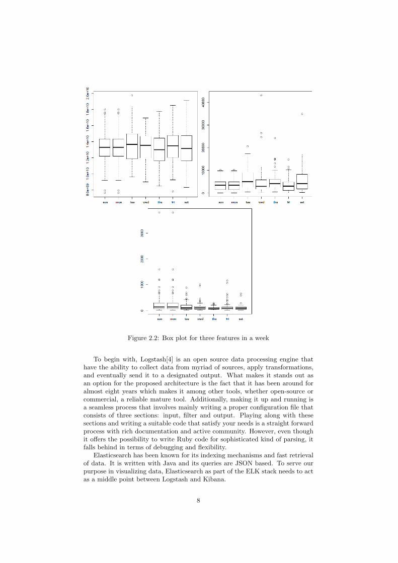
To give the reader another view using a more standard approach, we choseto plot three features using box plots. Using box plot helps to understand thedistribution of data and to provide descriptive analytics. They can be observedon figure 2.2 and you can notice the different behavior every feature exhibitsduring a week and that the values of a feature can be hundreds, thousands, oreven billions of units.

This section and the impact of its findings can be identified later on whenwe talk about standardization and clustering, especially when the number ofclusters is calculated as you can go back to figure 2.1 for comparison.

2.2 Architecture

The architecture consists of four main entities. They can be summarized ascollection and preprocessing entities, publish-subscribe messaging system, real-time and offline core processing engine, and data visualization pipeline. Tounderstand the connections between the architecture’s components and theirunderlying used technologies, refer to figure 2.3 below that depicts data flowwhile it is being processed from the time of collection until the final output.The core principles that have been considered throughout the whole designprocess is for the architecture to achieve three things: efficiency, scalability, andfault tolerance.

2.2.1 Collection and Visualization - ELK

ELK[17] is a stack that stands for three engines: Logstash as a data processingpipeline, Elasticsearch as a distributed system search engine, and Kibana as aweb interface that interacts directly with Elasticsearch to visualize the indexedpieces of data.

7

Figure 2.2: Box plot for three features in a week

To begin with, Logstash[4] is an open source data processing engine thathave the ability to collect data from myriad of sources, apply transformations,and eventually send it to a designated output. What makes it stands out asan option for the proposed architecture is the fact that it has been around foralmost eight years which makes it among other tools, whether open-source orcommercial, a reliable mature tool. Additionally, making it up and running isa seamless process that involves mainly writing a proper configuration file thatconsists of three sections: input, filter and output. Playing along with thesesections and writing a suitable code that satisfy your needs is a straight forwardprocess with rich documentation and active community. However, even thoughit offers the possibility to write Ruby code for sophisticated kind of parsing, itfalls behind in terms of debugging and flexibility.

Elasticsearch has been known for its indexing mechanisms and fast retrievalof data. It is written with Java and its queries are JSON based. To serve ourpurpose in visualizing data, Elasticsearch as part of the ELK stack needs to actas a middle point between Logstash and Kibana.

8

Figure 2.3: Data Flow Architecture

Kibana[3] is the last brick in the stack. It offers a seamless experience tovisualize and explore data stored in Elasticsearch. Its role in our design is toshow dashboards. These dashboards show anomaly scores, clusters distances,and essential core performance measurements. A threshold can be set so when-ever a value exceeds its limit, which in our case is the anomaly score, a visualrepresentation can be introduced e.g. red colored values, or an initiation of ascript that can alarm responsible personnel.

2.2.2 Normalization/Standardization - Python

It is fundamental to normalize/standardize data before feeding it to a cluster-ing algorithm, otherwise high positive/negative valued features will dominatethe process of model building, thus yielding to skewed results. The process ofscaling, namely squeezing data to fit the range between 0 and 1, is harmful con-sidering the changes that may occur on data distribution, therefore the values ofoutliers that need to be detected. The choice of using standardization 1 has beenobvious in this case, considering that all features will equally be represented tothe algorithm, and existed outliers will still exist.

One issue needs to be observed however. It is the fact that we do not have agrasp on a finite amount of data. The proposed system is designed to expect aninfinite stream. This means, standardization wise, a sliding window mechanismis needed, and that if the window is moving forward for each coming value ratherthan basing it on time, each value will be scaled differently. The impact of thatprocess is proportional to the window size and number of events per time unit.This will be discussed further in the evaluation section later on.

The standardization activity is accomplished using a python script wherefor each coming value, it stores it in a temporary file that holds recent received

1(Xi −mean)/standard deviation

9

values that constitute 24hours of events, updates it by removing the oldestrecord, standardize data, and eventually send the last record to output, whichin our case is to Kafka. This windowing activity has a window size of 97 and awindow movement that occurs for every received record. Notice here that thismechanism is a double edged sword. Moving the window for every record iscomputationally expensive; however, it assures that the process has an updatedview over exactly the last 24h of records. This is required due to the fact thatPMs over days do not exhibit similar behavior, and it offers better estimationsthan following the more common solution to move the window based on a time orrecords count interval. Considering that we have weekdays, weekends, holidays,and even more importantly, random public events and concerts imposes differentoverall behavior on a stream of data, therefore a high accurate standardizationprocess is required.

Nevertheless, in the light of the high cost the proposed standardization mech-anism may obtrude, a moving window every one hour can be reasonable but itis not evaluated nor is it discussed in this thesis.

It is worth mentioning that this component is deemed to be temporary untilSpark Structured Streaming allows for real-time learning and fitting models forwhich it’ll be discussed further in 2.2.4

2.2.3 Consumer/Producer broker - Kafka

The main purpose for putting up this entity is to avoid falling into back-pressureproblems and to establish a loosely coupled system. It is evident that Sparkis capable of processing huge loads of information. It is also true that in ourcurrent system the number of values for every 15 minutes does not exceed athousand. Nevertheless, since scalability has always been in most cases a crucialrequirement, an expectation of high loads of data coming through the systemis necessary. Also we need to consider that running many instances of a scriptas a producer is not usually a big issue if a well configured broker exists, buton the other hand demanding another instance of Spark to run on a deployedcluster in a production environment will cause much more hassle.

Another reason for the usage of Kafka is the fact that we need to assumethat each entity might fail or restarted while doing its job. For Spark to goup and running after a failure and start from where it has left off is usuallyaccomplished with the help of values like offsets. Kafka and Spark, our coreprocessing entity, are naturally connected with well established libraries andoffsets are sent within each message sent to Spark. So in any case Spark fails,Kafka is there to keep the state of the system saved.

2.2.4 Core Processing - Spark Structured Streaming

The choice of using Spark itself came after a handful of considerations. Simplyput, Spark[1] provides high speed processing engine compared to, for example,Hadoop MapReduce, ease of use bearing in mind its support for four dominantprogramming languages, generality considering that one application can pro-cess SQL queries, streaming, machine learning operations, and graph analyticsseamlessly, and finally, Spark does not need a specialized platform as it can runon Hadoop, Mesos, or as a standalone.

10

As for choosing Spark Structured Streaming, it was driven by multiple rea-sons. With the assumption that the reader heard of Spark Streaming since it hasbeen around for some time, the added values that Spark Structured Streamingadds on the table will only be mentioned.

Spark Structured Streaming is fairly new, and it has been introduced andunder extensive development since Spark 2.0 almost a year ago. It is a fault-tolerant stream processing engine that has DataFrames/Datasets in its coredata structure where calculations may be performed in SQL-like queries, and itis built on Spark SQL engine. This allows it to embrace the power of Spark’sSQL Catalyst Optimizer[10] where building extensible query optimizers is donewith the support of advanced programming languages properties. StructuredStreaming focuses on three aspects: Consistency, fault tolerance, and simplicity.By consistency, Spark assures that as long as all source inputs are generatingsequential streams, the output will take the same order. For fault tolerance,Spark saves the state of running processes in order to recover in case of failure.However, this not always true and it depends on what input sources or outputsinks are put in use. For example, using a socket input results in making Struc-tured Streaming incapable of recovering from input failures, unless it has beencoded by hand and offsets are included in received data. Lastly, its simplicitycomes from the fact that it uses Spark’s Dataframe and Dataset API makingthe process of initiating and processing queries a seamless one.

One might ask, what are its drawbacks? And why didn’t standardizationtake place in Spark Structured Streaming rather than assigning it to a Pythonscript? In fact, Spark Structured Streaming suffers from being incapable oflearning models on the fly. Namely, standardization in Spark is applied usingStandardScaler class. This process needs a prior knowledge of the data in hand,a model needs to be learned, and then for each coming value a transforma-tion can be achieved. For the time being, creating a machine learning pipelinefor Structure Streaming is not yet implemented, but there is already an opendiscussion on Jira[25] in order for such feature to see the light in the future.

In the proposed design, Spark has two tasks:

• In an offline manner: Learning and saving a normal model based on ahistorical set of data.

• In a real-time manner: Analyzing data received from Kafka, thereafterthrowing results into a file storage where checkpoints are defined in caseof failure.

These two tasks are discussed comprehensively in sections 2.3.1 and 2.3.2

2.3 Modeling and data Analytics

As discussed earlier, myriad number of algorithms and techniques are used toanalyze data, and in our case, the purpose is to detect unusual and unpredictedbehavior. As for K-means|| [12] algorithm, it is needless to say that numerousnumber of algorithms are more sophisticated compared to it, and in most casescomputationally more expensive e.g. Neural networks; however, knowing theextent to which we need such algorithms utterly depends on the use case inhand.

11

If we start from an extremely simplified approach in which the detectionprocess is for a single numerical dimensional space, statistical approaches inthat case helps in detecting and forecasting future values, for example, mov-ing average, moving median, and even a more sophisticated one, Autoregressiveintegrated moving average[14]. The problem escalates when the number of di-mensions increases, and the distribution and the values’ range at each dimensionare dissimilar. Then the scope of preferred algorithms expands to encompassdimensional reduction, clustering, and classification based algorithms amongmany others.

For this thesis, K-means|| is the chosen algorithm to be evaluated for ouruse case. The reasons that lie behind such a decision vary. Despite the fact thatnumerous papers examined streaming K-means clustering[6][9][21][32], to ourknowledge, the studies of K-means|| in a streaming environment for multivari-ate data as a holistic approach are limited in the scientific domain. Generally,the studies have been investigating and enhancing narrow pieces of the entirepicture of detecting abnormalities using the original K-means algorithm. Forexample, the focus has been to approximate and make a better performanceon iterative updates over K-means centroids [13] with the assumption that in-put data is well-clusterable and normalized. In other cases, studies proposedimprovements to real time queries for clusters’ state[36]. Lastly, Apache SparkStreaming offers, through out the support of mllib API, a well established im-plementation for streaming K-means. It is based on the mini-batch K-meansrule [31], and its control mechanism over estimates is achieved by what it callsa decay parameter. However, at the time of this writing it is not supported inSpark Structured Steamering for reasons mentioned earlier in 2.2.4. Further,our choice of employing K-means|| instead of the original K-means algorithm isdriven by several shortcomings the later suffers from, which will be discussedwhen building a normal model is examined in 2.3.1.

In short, this thesis tries to be more empirical than it is to be theoretical. Inthe next subsections, the two main tasks the core processing unit is responsiblefor are discussed and a simplified design is depicted in Figure 2.4

2.3.1 Normal behavior Model construction

In this process we try to tackle two problems. First we need to seek a generalizedmodel; namely, reaching a state where the entire set of values a day has is takeninto account. Secondly, it is imperative to avoid to mistakenly model outliers asnormal points. Especially taking into consideration the fact that K-means|| issignificantly sensitive to divergent inputs in a way that shifts computed centroidsdramatically.

In the beginning, we gathered the values of one week from the tenth to thesixteenth of December as training data. The available data that we had at thispoint represented the month of December, and our choice to pick that week wasfairly random; however, it was driven by our tendency to avoid abnormal days,that is public holidays.

In order to acquire a sense of how each day differ from another, three fea-tures2 are randomly chosen, and for each day of the week, they are plotted and

2In our use case, every record/value holds approximately a thousand features, and eachday is represented with a hundred values, roughly

12

Figure 2.4: Modeling And Data Analysis

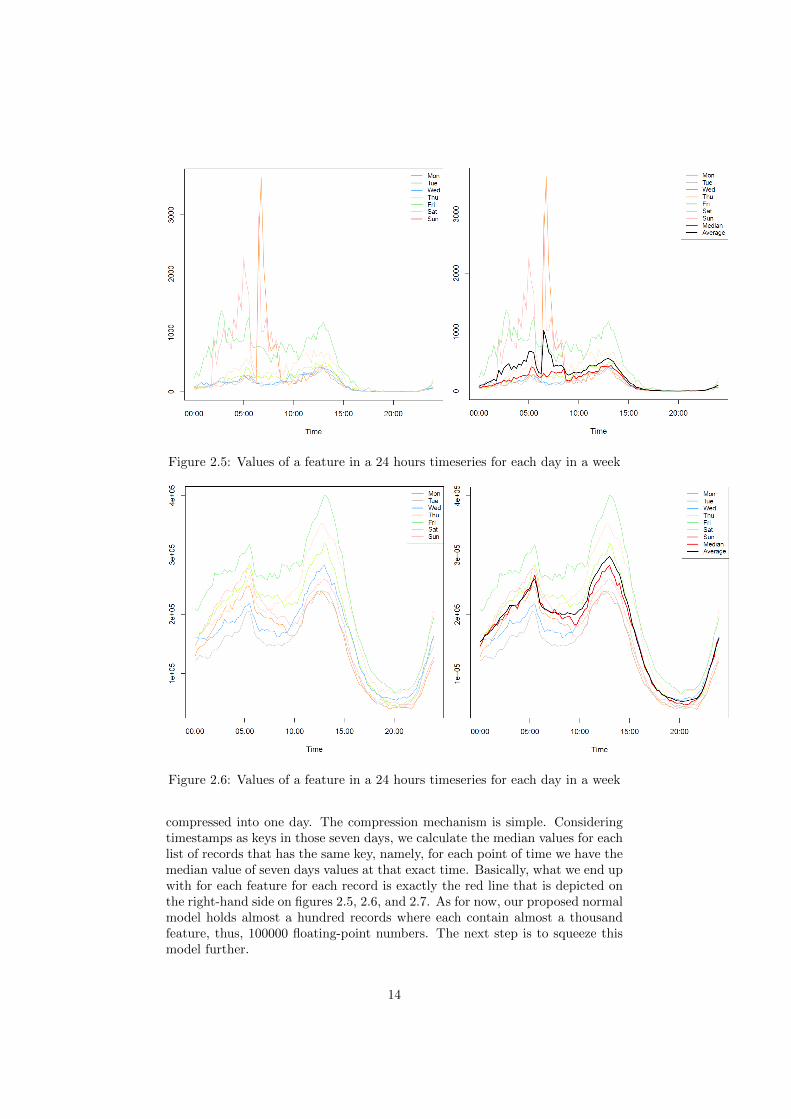
can be observed on Figure 2.5, 2.6, and 2.73. Each figure holds on the left-handside the values of a feature in a 24 hours timeseries for each day in a week, andon the right-hand side it holds the exact same values but added to them theiraverage and median charts. Notice on Figure 2.5 the non-stationary nature ofthe timeseries and that at least three days, which are Monday, Friday, and Sun-day, are divergent compared to the patterns that is followed by the other fourdays. You may also pay attention to the effect that the values have on theirassociated average and median values. The average chart is clearly more sen-sitive to high positive/negative values, while the median chart is more resilientto such changes. The same can be said for the rest of the figures.

This leads us to the first step in our model building. We take advantageof what robust statistics can offer. As for data that is derived from a widerange of probability distributions, going for traditional statical measurementsis not recommended nor is it considered accurate e.g. the usage of averageand standard deviation, as these measurement have a prior assumption overdata being normally distributed. That is when robust statistics steps in andmake an effort to deal with data regardless of its underlying distribution, and,unsurprisingly, catching outliers is one of its applications. In order to fulfillour endeavor to reach a normal model, the values of our training week shall be

3Please note that due to confidentiality constraints, the titles of the Y-axis have beenomitted

13

Figure 2.5: Values of a feature in a 24 hours timeseries for each day in a week

Figure 2.6: Values of a feature in a 24 hours timeseries for each day in a week

compressed into one day. The compression mechanism is simple. Consideringtimestamps as keys in those seven days, we calculate the median values for eachlist of records that has the same key, namely, for each point of time we have themedian value of seven days values at that exact time. Basically, what we end upwith for each feature for each record is exactly the red line that is depicted onthe right-hand side on figures 2.5, 2.6, and 2.7. As for now, our proposed normalmodel holds almost a hundred records where each contain almost a thousandfeature, thus, 100000 floating-point numbers. The next step is to squeeze thismodel further.

14

Figure 2.7: Values of a feature in a 24 hours timeseries for each day in a week

In general, K-means algorithm suffers from several setbacks:

• Sensitivity to outliers.

• Its initial random choice of centroids results in a high level of inaccuracy ofapproximations while taking into account the objective function, that is,minimizing WSSSE (Within Set Sum of Squared Error) in every cluster.

• Inability to dynamically figure out the approximate number of clusters.

The first obstacle is avoided appreciably by our previous step when we wentfor robust statistics. As for the second issue, in the learning and detection phase,K-means|| [12] is used. It is a scalable parallelized extension of K-means++.K-means++ [11] is in an extension of K-means, where in essence it is the samealgorithm; however it tries to overcome the issue of random centers initializationand it is ”O(log k)-competitive with the optimal clustering”[11]. Pay attentionto how K-means++ is distinguished from the traditional algorithm in Figure 2.8(steps 1a, 1b and 1c). Note that D(x) refers to the shortest distance between adata point and its closest center.

Figure 2.8: K-means++ Algorithm[11]

As for the last challenge, estimating what the best value of K can be achievedby several methods[2]. In this thesis, the elbow method is implemented, and also,

15

Figure 2.9: K-means Algorithm[11]

the study of our data in section 2.1 can be taken as a reference. Elbow method’smain objective is to find the optimal number of clusters by minimizing both, thenumber of clusters and the value of WSSSE (Within Set Sum of Squared Error).These two variables vary inversely, that is, a number of clusters that is equalto the number of data points results in a zero valued WSSSE, and the highestvalue of WSSSE occurs when there is only one cluster. The process is to runK-means|| and calculate WSSSE for every number of clusters, say, from one toten. Then by plotting the resulted data points, it is likely that we end up witha line chart that has an elbow shape, otherwise, we need to seek other means tofind the optimal number of clusters. In that chart, the point, where the elbowtakes its shape, has the best estimation of how many clusters the data has, thatis, where a sudden and significant decrease in WSSSE values variations occur.Running this technique on our recently computed model (A day that consists ofmedian values of a week form the tenth to the sixteenth of December) producedFigure 2.10

Figure 2.10: Elbow method for standardized data

The importance of standardization in our methodology process cannot beover emphasized. Note the difference between 2.10 which is based on standard-ized data and 2.11 which is based on raw data. Considering the fact that wedeal with multivariate data makes the second figure simply futile.

16

Figure 2.11: Elbow method for unstandardized data

It can be inferred by figure 2.10 that having four clusters is a reasonablenumber the we can use in training our final model.

Now, that the mentioned issues K-means suffers from are alleviated, it istime to go to the final step in our endeavor to acquire a normal behavior model.Basically, by implementing K-means|| on our day of median values with K equalsfour as input, our normal behavior model shall be ready.

2.3.2 K-means|| clustering and Outliers scoring

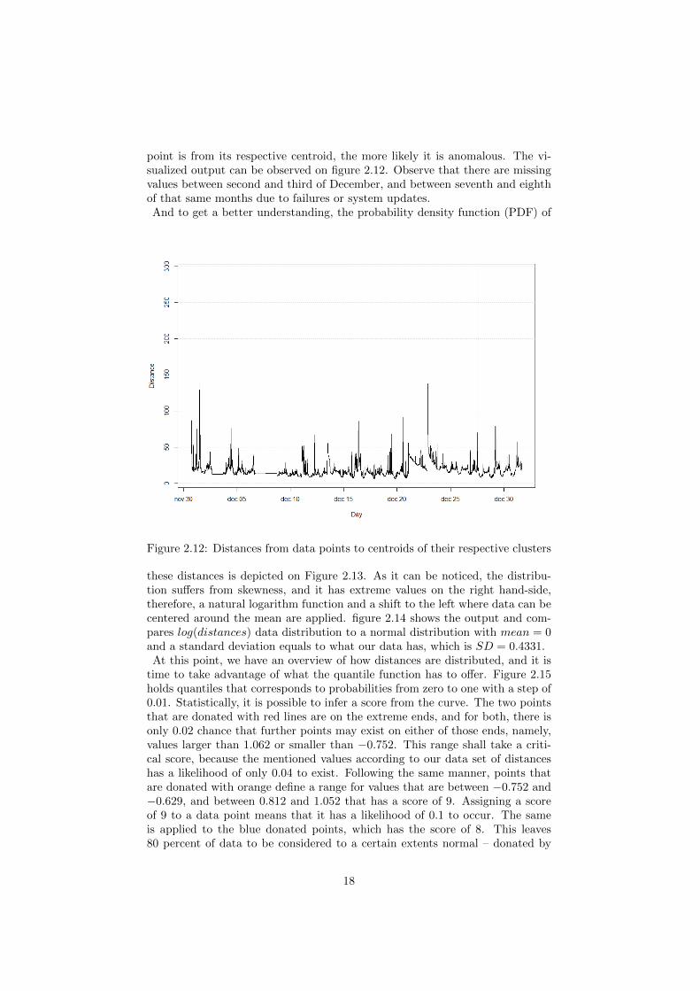
What was discussed in the previous section is done in an offline manner wherewe had a prior knowledge of the training set of data. However, in this sectionwe prepare the streaming system to receive records and analyze them.First, records are received and standardized by a Python script. The standard-ization is based on z-score and it occurs for each coming record. That is, foreach datum, the script updates a temporary set of values that constitutes thelast 24hours of data. It standardizes it based on its existent values. Finally, itsends the yielded standardized record to Kafka.Kafka holds data for a configured period of time with a configured number ofpartitions and topics. Within this period, consumers have the possibility tosubscribe to topics and request data from them. In our case, the consumer isSpark Structured Streaming; however, several consumers may exist.When Spark instance starts, the saved normal behavior model that has beencomputed will be loaded. Flowing records will be parsed, assigned to clusters,their distances to centroids (imported from the normal model) is calculated, anda score is given for each data point of how anomalous it may be.The process of making a scoring mechanism started by passing a set of a month’sdata to the system. This data holds nearly 2900 records where each has almosta thousand feature. The distances between each record and the centroid of theirrespective clusters are saved. The assumption here is that the further a data

17

point is from its respective centroid, the more likely it is anomalous. The vi-sualized output can be observed on figure 2.12. Observe that there are missingvalues between second and third of December, and between seventh and eighthof that same months due to failures or system updates.And to get a better understanding, the probability density function (PDF) of

Figure 2.12: Distances from data points to centroids of their respective clusters

these distances is depicted on Figure 2.13. As it can be noticed, the distribu-tion suffers from skewness, and it has extreme values on the right hand-side,therefore, a natural logarithm function and a shift to the left where data can becentered around the mean are applied. figure 2.14 shows the output and com-pares log(distances) data distribution to a normal distribution with mean = 0and a standard deviation equals to what our data has, which is SD = 0.4331.At this point, we have an overview of how distances are distributed, and it is

time to take advantage of what the quantile function has to offer. Figure 2.15holds quantiles that corresponds to probabilities from zero to one with a step of0.01. Statistically, it is possible to infer a score from the curve. The two pointsthat are donated with red lines are on the extreme ends, and for both, there isonly 0.02 chance that further points may exist on either of those ends, namely,values larger than 1.062 or smaller than −0.752. This range shall take a criti-cal score, because the mentioned values according to our data set of distanceshas a likelihood of only 0.04 to exist. Following the same manner, points thatare donated with orange define a range for values that are between −0.752 and−0.629, and between 0.812 and 1.052 that has a score of 9. Assigning a scoreof 9 to a data point means that it has a likelihood of 0.1 to occur. The sameis applied to the blue donated points, which has the score of 8. This leaves80 percent of data to be considered to a certain extents normal – donated by

18

Figure 2.13: Distances PDF

Figure 2.14: log(Distances) data distribution compared to a normal distribu-tion

green lines – but still has scores for further inspections. Please note that in anoptimal normal distribution, the score would be proportional to absolute values,and there is no need then to have low and high thresholds since both high andlow limits will be the same in their unsigned version. Meaning, for example,both absolute values of the two red points will be equal in that case.The output of this stage – which is the output of Spark Structured Streaming

– for each input record is normalized data accompanied by its distance from itsassociated centroid and its anomaly score.

19

Figure 2.15: Quantile function - Distances

20

Chapter 3

Experiments and Results

In this chapter, we test our proposed system against real and synthesized data.By the end, a set of results is presented to carry this thesis to the final chapterof results evaluation and discussion. The experiments start with real data andthen continues with synthesized ones in order to have a grasp on how change ofvalues will influence the anomaly score.While keeping that in mind, the tests will focus on high anomaly scores fre-quency, and how our score will react to synthetic anomalous data.

3.1 Real-Time Data Analysis

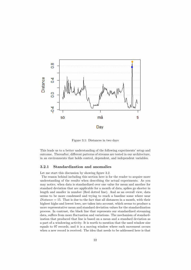
For this part, data of a two days has been gathered and fed to our streamingarchitecture. The data is for the 17th and 18th of September 2017. We considerthese two days a good choice for testing purposes as it includes working and non-working days, therefore, it is expected to incorporate high levels of fluctuationsand irregularities. Running our processes resulted in figure 3.1 As you maynotice, no red points are reported, one orange point for distances that has ananomaly score of nine, and a blue one for distances that has an anomaly scoreof eight. The higher, or lower, a value of a distance, the higher a score gets. It isup to business needs sensitivity to choose which points for which anomaly scoreto inspect, and up to the specialist based on his/her accumulated experience toconsider which scores need to be looked after. According to our observations, ascore of 10 implies a high level of necessity to initiate an investigation behindthe existence of that record. Orange colored points are anticipated to have lesssever consequences, and have a higher likelihood to appear as false positive-ish–since our system is not a decisive one and does not claim a 100% positivity– .As for the rest of points, the endeavor to catch a legit anomaly develops to beharder.

3.2 Synthesized Data Analysis

At this section we dive deep into how our system reacts to different patternsof inputs. By doing so, the reader will have a more profound insight on howefficient the system is. First, standardization is put under the spot light andanalyzed considering the distinction between offline and real-time processing.

21

Figure 3.1: Distances in two days

This leads us to a better understanding of the following experiments’ setup andoutcome. Thereafter, different patterns of streams are tested in our architecture,in an environments that holds control, dependent, and independent variables.

3.2.1 Standardization and anomalies

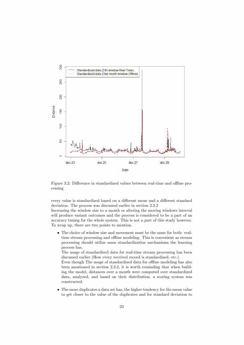
Let me start this discussion by showing figure 3.2.The reason behind including this section here is for the reader to acquire more

understanding of the results when describing the actual experiments. As youmay notice, when data is standardized over one value for mean and another forstandard deviation that are applicable for a month of data, spikes go shorter inlength and smaller in number (Red dotted line). And as an overall view, dataseems to be more condensed and trying to reach a baseline some where nearDistance = 15. That is due to the fact that all distances in a month, with theirhighest highs and lowest lows, are taken into account, which seems to produce amore representative mean and standard deviation values for the standardizationprocess. In contrast, the black line that represents our standardized streamingdata, suffers from more fluctuation and variations. The mechanism of standard-ization that produced that line is based on a mean and a standard deviation asa part of a windowing activity. It is worth to mention that the used window sizeequals to 97 records, and it is a moving window where each movement occurswhen a new record is received. The idea that needs to be addressed here is that

22

Figure 3.2: Difference in standardized values between real-time and offline pro-cessing

every value is standardized based on a different mean and a different standarddeviation. The process was discussed earlier in section 2.2.2Increasing the window size to a month or altering the moving windows intervalwill produce variant outcomes and the process is considered to be a part of anaccuracy tuning for the whole system. This is not a part of this study however.To wrap up, there are two points to mention.

• The choice of window size and movement must be the same for both: real-time stream processing and offline modeling. This is convenient as streamprocessing should utilize same standardization mechanisms the learningprocess has.The usage of standardized data for real-time stream processing has beendiscussed earlier (How every received record is standardized, etc.).Even though The usage of standardized data for offline modeling has alsobeen mentioned in section 2.3.2, it is worth reminding that when build-ing the model, distances over a month were computed over standardizeddata, analyzed, and based on their distribution, a scoring system wasconstructed.

• The more duplicates a data set has, the higher tendency for the mean valueto get closer to the value of the duplicates and for standard deviation to

23

reach zero. This fact will be addressed in following experiments in thecontext of data standardization.

3.2.2 Experiments

Several considerations have been taken into account.• The architectural environment shall be the same for all tests. Exactly as

depicted in Figure 2.3• As a control variable, a day in the test data set is passed into the system

in every test attempt in order for the standardization window to be fulland to be exactly the same in every test before feeding the system with-need to be tested- synthesized data.

• The mission is to send various synthesized records in each experiment andobserve the change on our dependent variable, the anomaly score, basedon independent variables, which are features, a record holds.

The tests have been executed on:• Red Hat Enterprise Linux Server. Release 6.4 (Santiago):

Kernel Linux 2.6.32-358.6.2.el6.x86 64• Memory: 126 GB• 18 Processiors: Intel(R) Xeon(R) CPU X5675 @ 3.07GHz

And the components of the architecture had the following SW version:• ELK: Logstash 5.5.0, Elasticsearch 5.5.0, and Kibana 5.5.0• Kafka 2.11-0.11.0.0• Zookeeper 3.4.10• Spark 2.2.0

As for the tests, we have a day which we will call (C).And a synthesized record that has an anomaly score of zero, which we will call(I0). And another, a score of ten, for which we will call (I10). The patternsare sent to the architecture as input, their output on Kibana is observed, andtheir anomaly score is recorded and will be called (D). This arrow (→ ) donatessending order. So A → B, means the sending starts from A and continues toB.

Patterns to be tested are:1. C → I0 (10 records)2. C → I10 (10 records)3. C → I0 → Customized I0 where 19 features1 out of the total 900 are

changed and assigned the maximum value they had in a month (10 records)4. C → I0 → Customized I0 where 19 features out of the total 900 are

changed and assigned the minimum values they had in a month (10 records)5. C → I0 → A data record that has the highest value for a Load Control

feature in a month with respect to all other features. (10 records)6. C → I0 → Customized I0 where one feature out of the total 900 that

has been known to be a constant zero for a whole month is changed to a1000 (10 records)

1These values are under a category concerned in Load Control

24

7. C → I0 → Customized I0 where 10 features out of the total 900 thathave been known to be constant zeros for a whole month are changed toa 1000 (10 records)

On table 3.1 you may spot the results. For each experiment, a sequence ofsaved anomaly scores is recorded. The first score in the sequence is associatedwith the first synthesized record that has been sent. So for example, in ex.1, thefirst score must be (0) as it is associated with I0, and afterwards, we observethe change of scores in the next 9 records.

Experiment No. Anomaly scores1 0, 0, 2, 3, 3, 4, 5, 5, 6, 62 10, 9, 8, 8, 8, 7, 7, 7, 6, 63 0, 6, 4, 2, 0, 0, 1, 2, 3, 4, 54 0, 5, 2, 1, 0, 1, 1, 2, 3, 4, 45 0, 9, 9, 8, 8, 7, 7, 7, 6, 6, 56 0, 2, 0, 1, 2, 3, 4, 4, 5, 6, 67 0, 8, 7, 6, 4, 3, 2, 1, 0, 0, 1

Table 3.1: Experiments’ Results

Experiments 1 and 2 are to test for scores consistency and to show stan-dardization effect. 3 and 4 are for observing the effect of features change onanomaly scores. 5 is similar to 3 and 4; however, instead of only changing aset of features out of the whole set, it takes into account the correlation of allfeatures. Lastly, 6 and 7 are to test for sensitivity and what effect changing aconstant will hold against anomaly scores.

25

Chapter 4

Evaluation and Discussion

As a general statement, the results are to a certain extent satisfactory, and nosurprising outcome can be noticed. However, several points need to be men-tioned.As for the experiments themselves, they are considered to be internally validconsidering the distinction between dependent, independent, and control vari-ables that has been accomplished. This was possible by starting every experi-ment from scratch, then feeding the system with predefined data, and eventuallymonitor the output. As for external validity, the tests comprised a set of pos-sibilities to test for consistency, variability, and sensitivity; however, within astreaming environment that consists of a standardization component for datathat has almost 900 features, it is not entirely correct to say that it is 100%externally valid. For example, altering our choices for what to use as controlvariables may produce slightly different output compared to that we acquired,mainly due to the sensitivity of the standardization process. But, through ourpractical experimentation, the overall conclusions that we reached, which willbe discussed in the following paragraphs, are externally valid.// In the firstpart, where two days data were injected as a stream into the system in orderto acquire a sort of a sense of how many possible anomalies our system willproduce, the results are convenient. These data points are not labeled and inour use case with the high number of features it is not possible to investigatethe authenticity of a possible anomaly. This makes our evaluation for this issueutterly based on our experience with data on one hand, and on related workon the other. It is also worth reminding that the assumption here is that thefurther a data point is from its centroid, the more anomalous it is likely to be.As for a score of 9 or 8, it is up to the analyst whether to dig deep into thoseoccurrences, however in our experimentation, specifically Ex.5, a score of 9 or 8does refer to a possible anomaly and it is encouraged to be investigated.For the analysis of synthesized data, experiments were conducted to observescores characteristics during operation time. As for scores consistency, extremescore values had the tendency to change score immediately after a second, or atmost a third, record is sent. In Ex.1, the score changed form 0 to 2 after threesent records. While in Ex.2, as soon as a second record was processed, the scorehad decreased by 1 from 10 to 9. As the sequence of records goes by, the scoredeviate dramatically, even though the record has the same values. The explana-tion here is that for every copy of record and due to the standardization process,

26

features approach the value of 0. And that comes as a result of a mean valuethat is getting closer to every feature value for each coming copy. So, dependingon centroids exact location in the denominational space in our normal model,the more copies of a record the system receive, the closer that record will getto the zeroed center of that dimensional space. We come to the conclusion thatin this setup, an analysis shall take interest in all high score values and mustnot assume that a decrease in a value of a score means a change of behavior.This is helpful for annoying situations were several alarms are triggered for thesame reason. In this process, a high score would trigger an alarm mechanism,thereafter a high score gets smoothed out if the anomaly persists. Neverthe-less, one can argue that this method is not entirely convenient, as this behaviorneeds to be learned by the analyst to understand the output. So if one desireto construct scores that are strongly connected to their associated records, thestandardization process needs to exclude all records that have high anomalyscores values. Therefore, for every record that has a high score, it shall not beincluded in the standardization process for the next coming record.As for Ex.3 and 4, changing 19 features, which constitutes 2.11% of the total900, to reach their maximum/minimum values they had in a month yielded poorresults, where a score of 6 or 5 is not truly considered an unusual behavior. Butit is worth to mention, that this is a part of an experiment and in a real worldscenario it is highly unlikely to have this kind of record due to the fact that these19 features are not independent from the rest of the measurements, and variouscorrelations exists among the whole set of features. This has led to Ex.5, wherewe try to consider these connections among features. In order to do so, insteadof only changing a set of features out of the whole set, the record takes intoaccount the correlation of all features. You may notice, the result for Ex.5 ismore convenient. A score of 9 gives an analyst the assumption that an anomalymay be present.Lastly, to test for sensitivity, a search for constant features was conducted.These features happen to a hold a value of 0. Before going further into eval-uations for Ex.6 and 7, one thing needs to be noted. You may need to knowthat the standardization for (0,0,0,1) is similar to (0,0,0,10000) which resultsto (-0.5,-0.5,-0.5,1.5). In other words, in a sequence of zeros, changing a valueto any real numbered value does not change the data distribution, thus, theoutput standardization will be the same. By projecting this on our two lastto-be-discussed experiments, we may conclude that the system shall not be ex-pected to notice a difference between high or low deviation from a constantzero, therefore for those two experiments we chose to change a feature to be a1000 arbitrarily, without expecting a different output if we chose otherwise. Asfor their result, the 6th, in which one feature was changed out of the total 900,did not contribute significantly in changing the score that increased from 0 to2. But in the 7th, changing ten constant features, which constitutes only 1,11%out of the whole features set, managed to push the score from 0 to 8. It canbe argued that it is not acceptable to give only a score of 8 to our synthesizedrecord considering that the changed 10 features were mostly constant the wholemonth, and any alteration in their values must yield to the highest anomalyscore possible.

27

Chapter 5

Conclusions and FutureWork

Those results helped shaping a structure of several ideas to improve them. Fur-ther experimentation shall be done on a standardization window, since it has acrucial part in the process. Since it is extremely sensitive to outliers, increasingits size to reach a limit where it is big enough in proportion to the numberof estimated anomalies is expected to produce better results, especially for thescore’s sensitivity part. Remember that the window size must be the same inthe learning and detecting phase. On a different thought, records that are asso-ciated with high scores must be excluded from the standardization process. Itis anticipated for this method to increase the detection efficiency.

28

References

[1] Apache spark - lightning-fast cluster computing. https://spark.apache.org/. [Online; accessed March 4, 2017].

[2] Cluster analysis in r: determine the optimal number of clusters -stack overflow. https://stackoverflow.com/questions/15376075/

cluster-analysis-in-r-determine-the-optimal-number-of-clusters/

15376462/#15376462. [Online; accessed April 26, 2017].

[3] Kibana: Explore, visualize, discover data — elastic. https://www.

elastic.co/products/kibana. [Online; accessed June 6, 2017].

[4] Logstash: Collect, parse, transform logs — elastic. https://www.elastic.co/products/logstash. [Online; accessed June 6, 2017].

[5] Sklearn preprocessing one hot encoder - documentation. http:

//scikit-learn.org/stable/modules/generated/sklearn.

preprocessing.OneHotEncoder.html, 2017. [Online; accessed Aug27, 2017].

[6] Marcel R. Ackermann, Marcus Martens, Christoph Raupach, KamilSwierkot, Christiane Lammersen, and Christian Sohler. Streamkm++: Aclustering algorithm for data streams. J. Exp. Algorithmics, 17:2.4:2.1–2.4:2.30, May 2012.

[7] Anishek Agarwal. Kappa architecture : In practice anishekagarwal medium. https://medium.com/@anishekagarwal/

kappa-architecture-in-practice-b0a4870f3da6, August 2016.[Online; accessed July 25, 2017].

[8] Subutai Ahmad and Scott Purdy. Real-time anomaly detection for stream-ing analytics. CoRR, abs/1607.02480, 2016.

[9] Nir Ailon, Ragesh Jaiswal, and Claire Monteleoni. Streaming k-meansapproximation. In Y. Bengio, D. Schuurmans, J. D. Lafferty, C. K. I.Williams, and A. Culotta, editors, Advances in Neural Information Pro-cessing Systems 22, pages 10–18. Curran Associates, Inc., 2009.

[10] Michael Armbrust. Making apache spark the fastest open source streamingengine - the databricks blog. https://databricks.com/blog/2017/06/

06/simple-super-fast-streaming-engine-apache-spark.html, June2017. [Online; accessed July 14, 2017].

29

[11] David Arthur and Sergei Vassilvitskii. K-means++: The advantages ofcareful seeding. In Proceedings of the Eighteenth Annual ACM-SIAM Sym-posium on Discrete Algorithms, SODA ’07, pages 1027–1035, Philadelphia,PA, USA, 2007. Society for Industrial and Applied Mathematics.

[12] Bahman Bahmani, Benjamin Moseley, Andrea Vattani, Ravi Kumar, andSergei Vassilvitskii. Scalable k-means++. Proc. VLDB Endow., 5(7):622–633, March 2012.

[13] Vladimir Braverman, Adam Meyerson, Rafail Ostrovsky, Alan Roytman,Michael Shindler, and Brian Tagiku. Streaming k-means on well-clusterabledata. In Proceedings of the Twenty-second Annual ACM-SIAM Symposiumon Discrete Algorithms, SODA ’11, pages 26–40, Philadelphia, PA, USA,2011. Society for Industrial and Applied Mathematics.

[14] Jason Brownlee. How to create an arima model fortime series forecasting with python - machine learn-ing mastery. https://machinelearningmastery.com/

arima-for-time-series-forecasting-with-python/, 2017 January.[Online; accessed October 22, 2017].

[15] B. Bse, B. Avasarala, S. Tirthapura, Y. Y. Chung, and D. Steiner. Detect-ing insider threats using radish: A system for real-time anomaly detectionin heterogeneous data streams. IEEE Systems Journal, 11(2):471–482, June2017.

[16] Varun Chandola, Arindam Banerjee, and Vipin Kumar. Anomaly detec-tion: A survey. ACM Comput. Surv., 41(3):15:1–15:58, July 2009.

[17] ELK. Powering data search, log analysis, analytics — elastic. https:

//www.elastic.co/products. [Online; accessed June 6, 2017].

[18] ANDRE ERIKSSON. A framework for anomaly detection withapplica-tions to sequences. Master’s thesis, KTH, School of Computer Science andCommunication (CSC), 2014.

[19] Reza Farivar and Bobby Evans. Q&a with bobby evans (ya-hoo) on storm - university of illinois at urbana-champaign — cours-era. https://www.coursera.org/learn/cloud-applications-part2/

lecture/bJ5Ee/3-3-6-q-a-with-bobby-evans-yahoo-on-storm, 2017.[Online; accessed March 25, 2017].

[20] Julien Forgeat. Data processing architectures lambda and kappa —ericsson research blog. https://www.ericsson.com/research-blog/

data-processing-architectures-lambda-and-kappa/, November 2015.[Online; accessed April 5, 2017].

[21] S. Guha, A. Meyerson, N. Mishra, R. Motwani, and L. O’Callaghan. Clus-tering data streams: Theory and practice. IEEE Transactions on Knowl-edge and Data Engineering, 15(3):515–528, May 2003.

[22] Victoria J. Hodge and Jim Austin. A survey of outlier detection method-ologies. Artificial Intelligence Review, 22(2):85–126, Oct 2004.

30

[23] IBM Big Data and Analytics Hub. Extracting business value from the 4v’s of big data. [Online; accessed June 27, 2017].

[24] Cisco Visual Networking Index. White paper: The zettabyte era: Trendsand analysis. Technical Report 1465272001812119, Cisco public, June 2017.

[25] JIRA. [spark-16424] add support for structured streaming to the ml pipelineapi - asf jira. https://issues.apache.org/jira/browse/SPARK-16424.[Online; accessed May 19, 2017].

[26] Nathan Marz. Lambda architecture lambda-architecture.net. http://

lambda-architecture.net/. [Online; accessed April 5, 2017].

[27] Kasey Panetta. Top trends in the gartner hype cy-cle for emerging technologies, 2017 - smarter with gart-ner. https://www.gartner.com/smarterwithgartner/

top-trends-in-the-gartner-hype-cycle-for-emerging-technologies-2017/,August 2017. [Online; accessed Sep 01, 2017].

[28] Jos Ramn Pasillas-Daz and Sylvie Ratt. An unsupervised approach forcombining scores of outlier detection techniques, based on similarity mea-sures. Electronic Notes in Theoretical Computer Science, 329(SupplementC):61 – 77, 2016. CLEI 2016 - The Latin American Computing Conference.

[29] Q. Plessis, M. Suzuki, and T. Kitahara. Unsupervised multi scale anomalydetection in streams of events. In 2016 10th International Conference onSignal Processing and Communication Systems (ICSPCS), pages 1–9, Dec2016.

[30] JEREMY RONK. Structured, semi structured and unstructured data— jeremy ronk. https://jeremyronk.wordpress.com/2014/09/01/

structured-semi-structured-and-unstructured-data/, SEPTEM-BRE 2014. [Online; accessed Aug 27, 2017].

[31] D. Sculley. Web-scale k-means clustering. In Proceedings of the 19th In-ternational Conference on World Wide Web, WWW ’10, pages 1177–1178,New York, NY, USA, 2010. ACM.

[32] Michael Shindler, Alex Wong, and Adam Meyerson. Fast and accuratek-means for large datasets. In Proceedings of the 24th International Con-ference on Neural Information Processing Systems, NIPS’11, pages 2375–2383, USA, 2011. Curran Associates Inc.

[33] Letham B Taylor SJ. Forecasting at scale. PeerJ Preprints 5:e3190v2,2017.

[34] Owen Vallis, Jordan Hochenbaum, and Arun Kejariwal. A novel techniquefor long-term anomaly detection in the cloud. In Proceedings of the 6thUSENIX Conference on Hot Topics in Cloud Computing, HotCloud’14,pages 15–15, Berkeley, CA, USA, 2014. USENIX Association.

[35] Laurens van der Maaten. t-sne. https://lvdmaaten.github.io/tsne/,2017. [Online; accessed April 16, 2017].

31

[36] Y. Zhang, K. Tangwongsan, and S. Tirthapura. Streaming k-means clus-tering with fast queries. In 2017 IEEE 33rd International Conference onData Engineering (ICDE), pages 449–460, April 2017.

32

TRITA EE 2017:177

ISSN 1653-5146

www.kth.se