ANOVA ‐ Analysis of Variance

ANOVA ‐ Analysis of Variance

• Extends independent‐samples t test

ANOVA ‐ Analysis of Variance

• Extends independent‐samples t test

• Compares the means of groups of independent observations

ANOVA ‐ Analysis of Variance

• Extends independent‐samples t test

• Compares the means of groups of independent observations

– Don’t be fooled by the name.  ANOVA does not compare variances.

ANOVA ‐ Analysis of Variance

• Extends independent‐samples t test

• Compares the means of groups of independent observations

– Don’t be fooled by the name.  ANOVA does not compare variances.

• Can compare more than two groups

ANOVA – Null and Alternative Hypotheses

Say the sample contains K independent groups

ANOVA – Null and Alternative Hypotheses

Say the sample contains K independent groups

• ANOVA tests the null hypothesis 

H0: μ1 = μ2 = … = μK

– That is, “the group means are all equal”

ANOVA – Null and Alternative Hypotheses

Say the sample contains K independent groups

• ANOVA tests the null hypothesis 

H0: μ1 = μ2 = … = μK

– That is, “the group means are all equal”

• The alternative hypothesis is

H1: μi ≠ μj for some i, j

– or,  “the group means are not all equal”

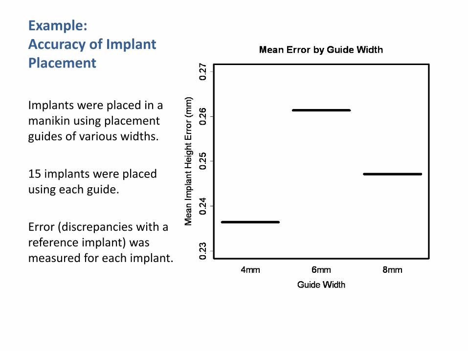
Example:  Accuracy of Implant Placement

Implants were placed in a manikin using placement guides of various widths.

15 implants were placed using each guide.

Error (discrepancies with a reference implant) was measured for each implant. 

Example:  Accuracy of Implant Placement

The overall mean of the entire sample was 0.248 mm.

This is called the “grand” mean, and is often denoted by       . 

If H0 were true then we’d expect the group means to be close to the grand mean.

X

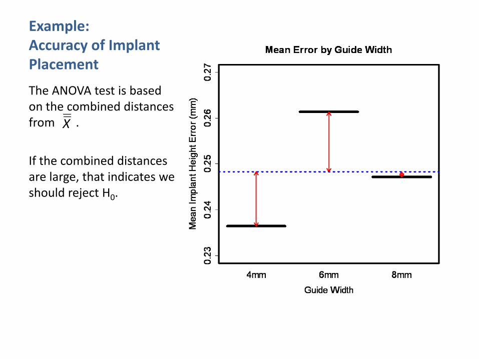
Example:  Accuracy of Implant Placement

The ANOVA test is based on the combined distances from       .

If the combined distances are large, that indicates we should reject H0.

X

The Anova Statistic

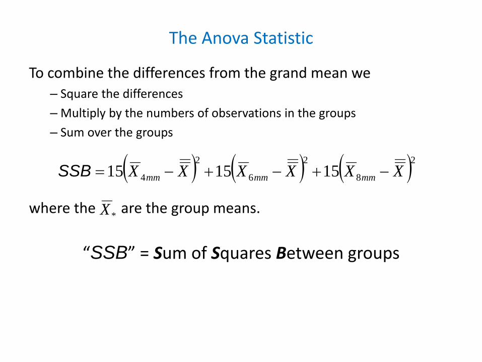
To combine the differences from the grand mean we – Square the differences 

– Multiply by the numbers of observations in the groups

– Sum over the groups

where the       are the group means.

“SSB” = Sum of Squares Between groups

( ) ( ) ( )28

2

6

2

4 151515 XXXXXX mmmmmm −+−+−= SSB

*X

The Anova Statistic

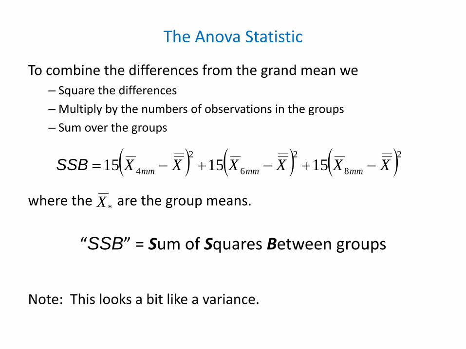
To combine the differences from the grand mean we – Square the differences 

– Multiply by the numbers of observations in the groups

– Sum over the groups

where the       are the group means.

“SSB” = Sum of Squares Between groups

Note:  This looks a bit like a variance.

( ) ( ) ( )28

2

6

2

4 151515 XXXXXX mmmmmm −+−+−= SSB

*X

How big is big?

• For the Implant Accuracy Data, SSB = 0.0047

• Is that big enough to reject H0?

• As with the t test, we compare the statistic to the variability of the individual observations.

• In ANOVA the variability is estimated by the Mean Square Error, or MSE

MSEMean Square Error

The Mean Square Error is a measure of the variability after the group effects have been taken into account.

where xij is the ith

observation in the jth

group.  

( )∑∑ −−

=j i

jij XxKN

MSE 21

MSEMean Square Error

The Mean Square Error is a measure of the variability after the group effects have been taken into account.

where xij is the ith

observation in the jth

group.  

( )∑∑ −−

=j i

jij XxKN

MSE 21

MSEMean Square Error

The Mean Square Error is a measure of the variability after the group effects have been taken into account.

Note that the variation of the means seems quite small compared to the variance of observations within groups

( )∑∑ −−

=j i

jij XxKN

MSE 21

Notes on MSE

• If there are only two groups, the MSE is equal to the pooled estimate of variance used in the equal‐variance t test.

• ANOVA assumes that all the group variances are equal.

• Other options should be considered if group variances differ by a factor of 2 or more.

ANOVA F Test

• The ANOVA F test is based on the F statistic

where K is the number of groups.

• Under H0 the F statistic has an “F” distribution, with K‐1 and N‐K degrees of freedom (N is the total number of observations)

MSEKSSB

F)1( −

=

Implant Data:F test p‐value

To get a p‐value we compare our F statistic to an F(2, 42) distribution.

Implant Data:F test p‐value

To get a p‐value we compare our F statistic to an F(2, 42) distribution.

In our example

211.420467.20047.==F

Implant Data:F test p‐value

To get a p‐value we compare our F statistic to an F(2, 42) distribution.

In our example

The p‐value is 

211.420467.20047.==F

( ) 81.0211(2,42) =>  .  FP

ANOVA Table

Sum of Squares df

Mean Square F Sig.

Between Groups .005 2 .002 .211 .811

Within Groups .466 42 .011

Total .470 44

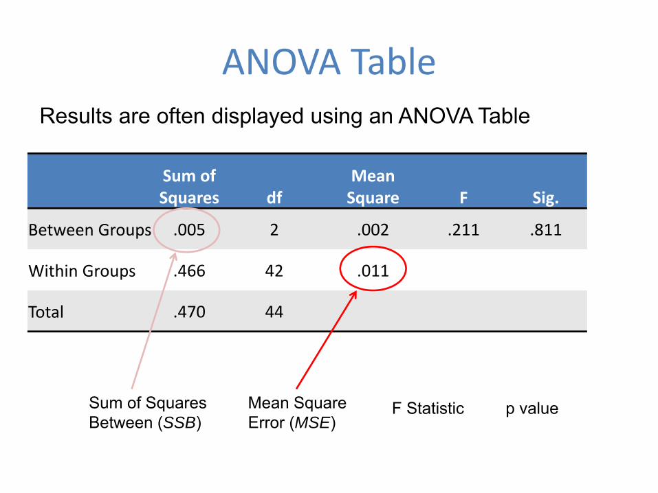
Results are often displayed using an ANOVA Table

ANOVA Table

Sum of Squares df

Mean Square F Sig.

Between Groups .005 2 .002 .211 .811

Within Groups .466 42 .011

Total .470 44

Results are often displayed using an ANOVA Table

Sum of Squares Between (SSB)

Mean Square Error (MSE)

F Statistic p value

Pop Quiz!: Where are the following quantities presented in this table?

ANOVA Table

Sum of Squares df

Mean Square F Sig.

Between Groups .005 2 .002 .211 .811

Within Groups .466 42 .011

Total .470 44

Results are often displayed using an ANOVA Table

Sum of Squares Between (SSB)

Mean Square Error (MSE)

F Statistic p value

ANOVA Table

Sum of Squares df

Mean Square F Sig.

Between Groups .005 2 .002 .211 .811

Within Groups .466 42 .011

Total .470 44

Results are often displayed using an ANOVA Table

Sum of Squares Between (SSB)

Mean Square Error (MSE)

F Statistic p value

ANOVA Table

Sum of Squares df

Mean Square F Sig.

Between Groups .005 2 .002 .211 .811

Within Groups .466 42 .011

Total .470 44

Results are often displayed using an ANOVA Table

Sum of Squares Between (SSB)

Mean Square Error (MSE)

F Statistic p value

ANOVA Table

Sum of Squares df

Mean Square F Sig.

Between Groups .005 2 .002 .211 .811

Within Groups .466 42 .011

Total .470 44

Results are often displayed using an ANOVA Table

Sum of Squares Between (SSB)

Mean Square Error (MSE)

F Statistic p value

Post Hoc Tests

Sum of Squares df

Mean Square F Sig.

Between Groups

33383 3 11128 5.1 .002

Within Groups

4417119 2007 2201

Total 4450502 2010

NHANES I data, women 40-60 yrs old. Compare cholesterol between periodontal groups.

The ANOVA shows good evidence (p = 0.002) that the means are not all the same.

Which means are different?

Can directly compare the subgroups using “post hoc” tests.

Least Significant Difference test

Sum of Squares df

Mean Square F Sig.

Between Groups

33383 3 11128 5.1 .002

Within Groups

4417119 2007 2201

Total 4450502 2010

The most simple post hoc test is called the Least Significant Difference Test.

The computation is very similar to the equal-variance t test.

Compute an equal-variance t test, but replace the pooled variance (s2) with the MSE.

N MeanStd. 

DeviationHealthy 802 221.5 46. 2

Gingivitis 490 223.5 45.3

Periodontitis 347 227.3 48.9

Edentulous 372 232.4 48. 8

Least Significant Difference Test: Examples

Sum of Squares df

Mean Square F Sig.

Between Groups

33383 3 11128 5.1 .002

Within Groups

4417119 2007 2201

Total 4450502 2010

Compare Healthy group to Periodontitis group:

Compare Gingivitis group to Periodontitis group:

N MeanStd. 

DeviationHealthy 802 221.5 46. 2

Gingivitis 490 223.5 45.3

Periodontitis 347 227.3 48.9

Edentulous 372 232.4 48. 8

( )92.1

347180212201

3.2275.221−=

+−

=T

055.0)92.1(2 1147 =>⋅= tPp

( )15.1

347149012201

3.2275.223−=

+−

=T

25.0)15.1(2 835 =>⋅= tPp

Post Hoc Tests: Multiple Comparisons

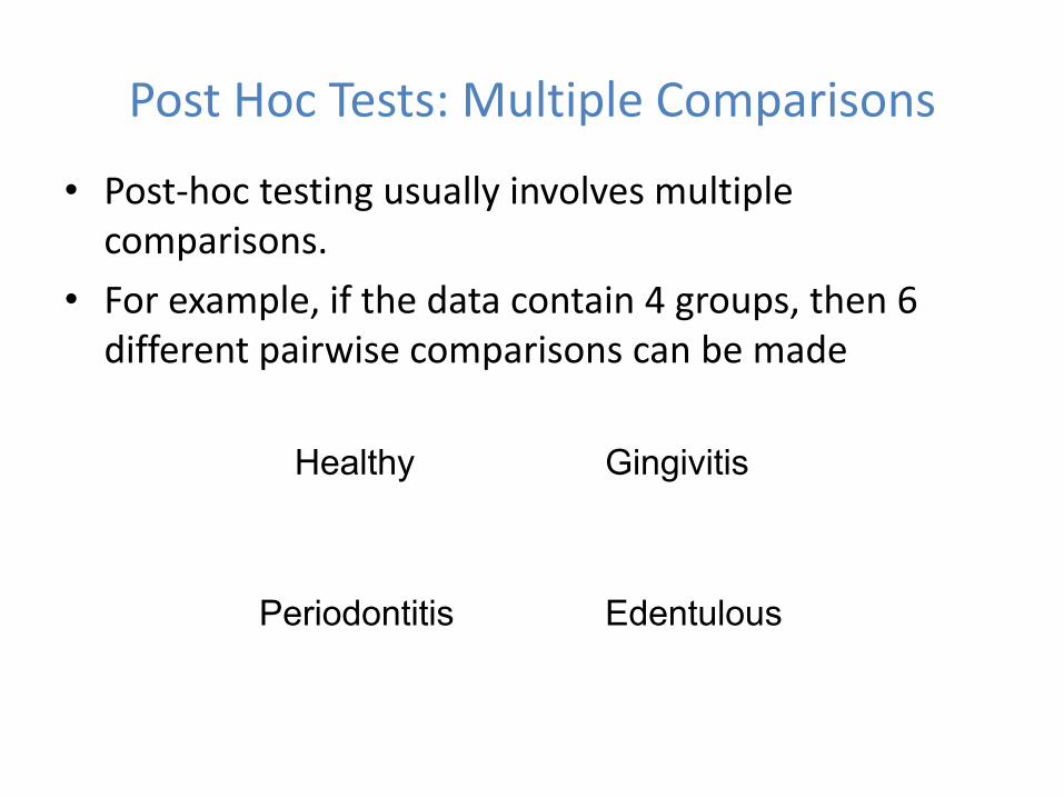
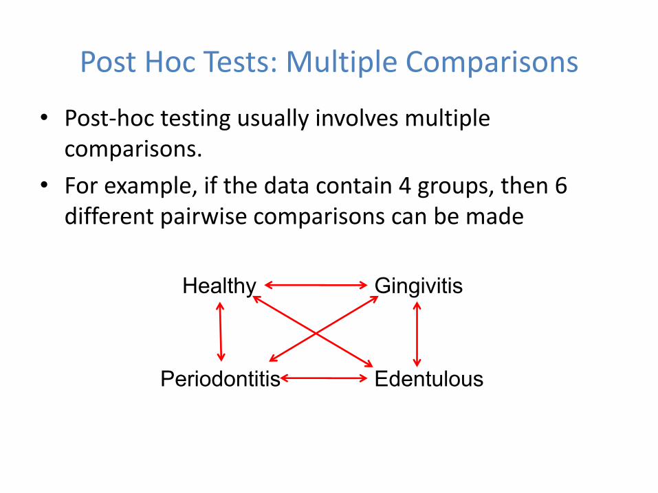
• Post‐hoc testing usually involves multiple comparisons.

Post Hoc Tests: Multiple Comparisons

• Post‐hoc testing usually involves multiple comparisons.

• For example, if the data contain 4 groups, then 6 different pairwise comparisons can be made

Healthy Gingivitis

Periodontitis Edentulous

Post Hoc Tests: Multiple Comparisons

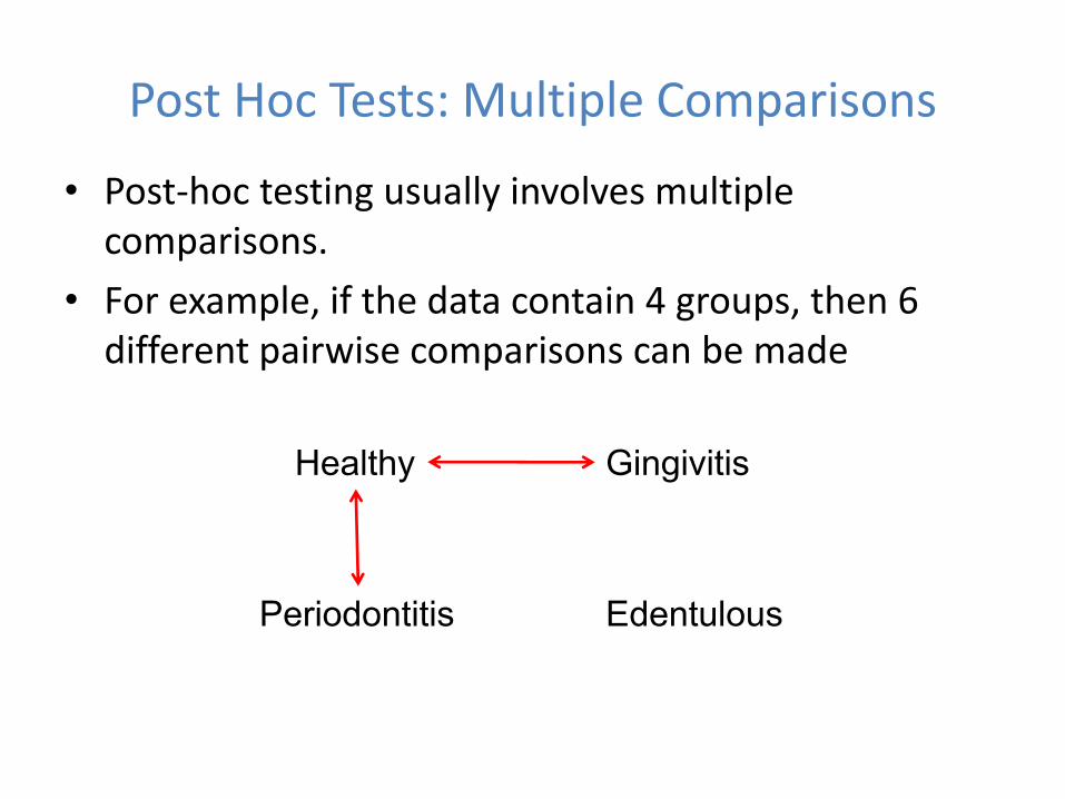
• Post‐hoc testing usually involves multiple comparisons.

• For example, if the data contain 4 groups, then 6 different pairwise comparisons can be made

Healthy Gingivitis

Periodontitis Edentulous

Post Hoc Tests: Multiple Comparisons

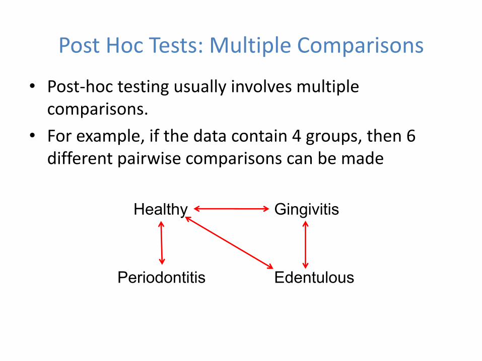
• Post‐hoc testing usually involves multiple comparisons.

• For example, if the data contain 4 groups, then 6 different pairwise comparisons can be made

Healthy Gingivitis

Periodontitis Edentulous

Post Hoc Tests: Multiple Comparisons

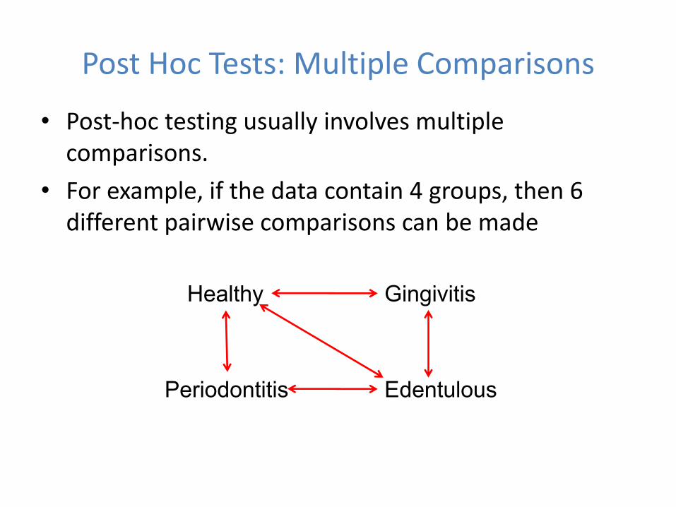
• Post‐hoc testing usually involves multiple comparisons.

• For example, if the data contain 4 groups, then 6 different pairwise comparisons can be made

Healthy Gingivitis

Periodontitis Edentulous

Post Hoc Tests: Multiple Comparisons

• Post‐hoc testing usually involves multiple comparisons.

• For example, if the data contain 4 groups, then 6 different pairwise comparisons can be made

Healthy Gingivitis

Periodontitis Edentulous

Post Hoc Tests: Multiple Comparisons

• Post‐hoc testing usually involves multiple comparisons.

• For example, if the data contain 4 groups, then 6 different pairwise comparisons can be made

Healthy Gingivitis

Periodontitis Edentulous

Post Hoc Tests: Multiple Comparisons

• Post‐hoc testing usually involves multiple comparisons.

• For example, if the data contain 4 groups, then 6 different pairwise comparisons can be made

Healthy Gingivitis

Periodontitis Edentulous

Post Hoc Tests: Multiple Comparisons

• Each time a hypothesis test is performed at significance level α, there is probability α of rejecting in error.

• Performing multiple tests increases the chances of rejecting in error at least once.

Post Hoc Tests: Multiple Comparisons

• Each time a hypothesis test is performed at significance level α, there is probability α of rejecting in error.

• Performing multiple tests increases the chances of rejecting in error at least once.

• For example:– if you did 6 independent hypothesis tests at the α = 0.05

Post Hoc Tests: Multiple Comparisons

• Each time a hypothesis test is performed at significance level α, there is probability α of rejecting in error.

• Performing multiple tests increases the chances of rejecting in error at least once.

• For example:– if you did 6 independent hypothesis tests at the α = 0.05

– If, in truth, H0 were true for all six.

Post Hoc Tests: Multiple Comparisons

• Each time a hypothesis test is performed at significance level α, there is probability α of rejecting in error.

• Performing multiple tests increases the chances of rejecting in error at least once.

• For example:– if you did 6 independent hypothesis tests at the α = 0.05

– If, in truth, H0 were true for all six.

– The probability that at least one test rejects H0 is 26%

Post Hoc Tests: Multiple Comparisons

• Each time a hypothesis test is performed at significance level α, there is probability α of rejecting in error.

• Performing multiple tests increases the chances of rejecting in error at least once.

• For example:– if you did 6 independent hypothesis tests at the α = 0.05

– If, in truth, H0 were true for all six.

– The probability that at least one test rejects H0 is 26%

– P(at least one rejection) = 1‐P(no rejections) = 1‐.956 = .26

Bonferroni Correction for Multiple Comparisons

• The Bonferroni correction is a simple way to adjust for the multiple comparisons.

Bonferroni Correction• Perform each test at significance level α.

• Multiply each p-value by the number of tests performed.

• The overall significance level (chance of any of the tests rejecting in error) will be less than α.

Example: Cholesterol Data post‐hoc comparisons

Group 1 Group 2

Mean Difference (Group 1 -Group 2)

Least Significant Difference

p-valueBonferroni

p-valueHealthy Gingivitis -2.0 .46 1.0Healthy Periodontitis -5.8 .055 .330Healthy Edentulous -10.9 .00021 .00126Gingivitis Periodontitis -3.9 .25 1.0Gingivitis Edentulous -8.9 .0056 .0336Periodontitis Edentulous -5.1 .147 .88

Example: Cholesterol Data post‐hoc comparisons

Conclusion: The Edentulous group is significantly different than the Healthy group and the Gingivitis group (p < 0.05), after adjustment for multiple comparisons

Group 1 Group 2

Mean Difference (Group 1 -Group 2)

Least Significant Difference

p-valueBonferroni

p-valueHealthy Gingivitis -2.0 .46 1.0Healthy Periodontitis -5.8 .055 .330Healthy Edentulous -10.9 .00021 .00126Gingivitis Periodontitis -3.9 .25 1.0Gingivitis Edentulous -8.9 .0056 .0336Periodontitis Edentulous -5.1 .147 .88