31
Multiple comparisons Modeling and ANOVA Multiple comparisons and ANOVA Patrick Breheny April 19 Patrick Breheny STA 580: Biostatistics I 1/31

Multiple comparisonsModeling and ANOVA
Multiple comparisons and ANOVA
Patrick Breheny
April 19
Patrick Breheny STA 580: Biostatistics I 1/31

Multiple comparisonsModeling and ANOVA
IntroductionThe Bonferroni correctionThe false discovery rate
Multiple comparisons
So far in this class, I’ve painted a picture of research in whichinvestigators set out with one specific hypothesis in mind,collect a random sample, then perform a hypothesis test
Real life is a lot messier
Investigators often test dozens of hypotheses, and don’talways decide on those hypotheses before they have looked attheir data
Hypothesis tests and p-values are much harder to interpretwhen multiple comparisons have been made
Patrick Breheny STA 580: Biostatistics I 2/31

Multiple comparisonsModeling and ANOVA
IntroductionThe Bonferroni correctionThe false discovery rate
Environmental health emergency . . .
As an example, suppose we see five cases of a certain type ofcancer in the same neighborhood
Suppose also that the probability of seeing a single case inneighborhood this size is 1 in 10
If the cases arose independently (our null hypothesis), thenthe probability of seeing three cases in the neighborhood in asingle year is
(110
)5= .00001
This looks like pretty convincing evidence that chance alone isan unlikely explanation for the outbreak, and that we shouldlook for a common cause
This type of scenario occurs all the time, and suspicion isusually cast on a local industry and their waste disposalpractices, which may be contaminating the air, ground, orwater
Patrick Breheny STA 580: Biostatistics I 3/31
Multiple comparisonsModeling and ANOVA
IntroductionThe Bonferroni correctionThe false discovery rate
. . . or coincidence?
But there are a lot of neighborhoods and a lot of types ofcancer
Suppose we were to carry out such a hypothesis test for100,000 different neighborhoods and 100 different types ofcancer
Then we would expect (100, 000)(100)(.00001) = 100 of thesetests to have p-values below .00001 just by random chance
As a result, further investigations by epidemiologists and otherpublic health officials rarely succeed in finding a commoncause
The lesson: if you keep testing null hypotheses, sooner orlater, you’ll find significant differences regardless of whether ornot one exists
Patrick Breheny STA 580: Biostatistics I 4/31

Multiple comparisonsModeling and ANOVA
IntroductionThe Bonferroni correctionThe false discovery rate
Breast cancer study
If an investigator begins with a clear set of hypotheses inmind, however, and these hypotheses are independent, thenthere are methods for carrying out tests while adjusting formultiple comparisons
For example, consider a study done at the National Institutesof Health to find genes associated with breast cancer
They looked at 3,226 genes, carrying out a two-sample t-testfor each gene to see if the expression level of the gene differedbetween women with breast cancer and healthy controls (i.e.,they got 3,226 p-values)
Patrick Breheny STA 580: Biostatistics I 5/31
Multiple comparisonsModeling and ANOVA
IntroductionThe Bonferroni correctionThe false discovery rate
Probability of a single mistake
If we accepted p < .05 as convincing evidence, what is theprobability that we would make at least one mistake?
P (At least one error) = 1 − P (All correct)
≈ 1 − .953,226
≈ 1
If we want to keep our overall probability of making a type Ierror at 5%, we need to require p to be much lower
Patrick Breheny STA 580: Biostatistics I 6/31

Multiple comparisonsModeling and ANOVA
IntroductionThe Bonferroni correctionThe false discovery rate
The Bonferroni correction
Instead of testing each individual hypothesis at α = .05, wewould have to compare our p-values to a new, lower value α∗,where
α∗ =α
h
where h is the number of hypothesis tests that we areconducting (this approach is called the Bonferroni correction)
For the breast cancer study, α∗ = .000015
Note that it is still possible to find significant evidence of agene-cancer association, but much more evidence is needed toovercome the multiple testing
Patrick Breheny STA 580: Biostatistics I 7/31

Multiple comparisonsModeling and ANOVA
IntroductionThe Bonferroni correctionThe false discovery rate
False discovery rate
Another way to adjust for multiple hypothesis tests is the falsediscovery rate
Instead of trying to control the overall probability of a type Ierror, the false discovery rate controls the proportion ofsignificant findings that are type I errors
If a cutoff of α for the individual hypothesis tests results in ssignificant findings, then the false discovery rate is:
FDR =hα
s
Patrick Breheny STA 580: Biostatistics I 8/31

Multiple comparisonsModeling and ANOVA
IntroductionThe Bonferroni correctionThe false discovery rate
False discovery rate applied to the breast cancer studyproblem
So for example, in the breast cancer study, p < .01 for 207 ofthe hypothesis tests
By chance, we would have expected 3226(.01) = 32.26significant findings by chance alone
Thus, the false discovery rate for this p-value cutoff is
FDR =32.26
207= 15.6%
We can expect roughly 15.6% of these 207 genes to bespurious results, linked to breast cancer only by chancevariability
Patrick Breheny STA 580: Biostatistics I 9/31

Multiple comparisonsModeling and ANOVA
IntroductionThe Bonferroni correctionThe false discovery rate
Breast cancer study: Visual idea of FDR
p
Fre
quen
cy
0.0 0.2 0.4 0.6 0.8 1.0
010
020
030
0
Patrick Breheny STA 580: Biostatistics I 10/31

Multiple comparisonsModeling and ANOVA
IntroductionThe Bonferroni correctionThe false discovery rate
Breast cancer study: FDR vs. α
0.00 0.01 0.02 0.03 0.04 0.05
0.00
0.05
0.10
0.15
0.20
0.25
0.30
α
FD
R
Patrick Breheny STA 580: Biostatistics I 11/31

Multiple comparisonsModeling and ANOVA
IntroductionThe Bonferroni correctionThe false discovery rate
Other examples
The issue of multiple testing comes up a lot – for example,
Subgroup analyses: separately analyses of the subjects by sexor by age group or patients with severe disease/mild disease
Multiple outcomes: we might collect data on whether thepatients died, how long the patients were in the intensive careunit, how long they required mechanical ventilation, howmany days they required treatment with vasopressors, etc.
Multiple risk factors for a single outcome
Patrick Breheny STA 580: Biostatistics I 12/31
Multiple comparisonsModeling and ANOVA
IntroductionExplained and unexplained variability
Comparing multiple groups
A different kind of multiple comparisons issue arises whenthere is only one outcome, but there are multiple groupspresent in the study
For example, in the tailgating study, we compared illegal drugusers with non-illegal drug users
However, there were really four groups: individuals who usemarijuana, individuals who use MDMA (ecstasy), individualswho drink alcohol, and drug-free individuals
Patrick Breheny STA 580: Biostatistics I 13/31
Multiple comparisonsModeling and ANOVA
IntroductionExplained and unexplained variability
The problem with multiple t-tests
We talked about how to analyze one-sample studies andtwo-sample studies; how do we test for significant differencesin a four-sample study?
We could carry out 6 different t/Mann-Whitney tests (one foreach two-group comparison), but as we have seen, this willincrease our type I error rate (unless we correct for it)
Instead, it is desirable to have a method for testing the singlehypothesis that the mean of all four groups is the same
To do this, however, we will need a different approach to thanthe ones we have used so far in this course: we will need tobuild a statistical model
Patrick Breheny STA 580: Biostatistics I 14/31
Multiple comparisonsModeling and ANOVA
IntroductionExplained and unexplained variability
The philosophy of statistical models
There are unexplained phenomena that occur all around us,every day: Why do some die while others live? Why does onetreatment work better on some, and a different treatment forothers? Why do some tailgate the car in front of them whileothers follow at safer distances?
Try as hard as we may, we will never understand any of thesethings in their entirety; nature is far too complicated to everunderstand perfectly
There will always be variability that we cannot explain
The best we can hope to do is to develop an oversimplifiedversion of how the world works that explains some of thatvariability
Patrick Breheny STA 580: Biostatistics I 15/31
Multiple comparisonsModeling and ANOVA
IntroductionExplained and unexplained variability
The philosophy of statistical models (cont’d)
This oversimplified version of how the world works is called amodel
The point of a model is not to accurately represent exactlywhat is going on in nature; that would be impossible
The point is to develop a model that will help us tounderstand, to predict, and to make decisions in the presenceof this uncertainty – and some models are better at this thanothers
The philosophy of a statistical model is summarized in afamous quote by the statistician George Box: “All models arewrong, but some are useful”
Patrick Breheny STA 580: Biostatistics I 16/31
Multiple comparisonsModeling and ANOVA
IntroductionExplained and unexplained variability
Residuals
What makes one model better than another is the amount ofvariability it is capable of explaining
Let’s return to our tailgating study: the simplest model is thatthere is one mean tailgating distance for everyone and thateverything else is inexplicable variability
Using this model, we would calculate the mean tailgatingdistance for our sample
Each observation yi will deviate from this mean by someamount ri: ri = yi − y
The values ri are called the residuals of the model
Patrick Breheny STA 580: Biostatistics I 17/31

Multiple comparisonsModeling and ANOVA
IntroductionExplained and unexplained variability
Residual sum of squares
We can summarize the size of the residuals by calculating theresidual sum of squares:
RSS =∑i
r2i
The residual sum of squares is a measure of the unexplainedvariability that a model leaves behind
For example, the residual sum of squares for the simple modelof the tailgating data is (−23.1)2 + (−2.1)2 + . . . = 230, 116.1
Note that residual sum of squares doesn’t mean much byitself, because it depends on the sample size and the scale ofthe outcome, but it has meaning when compared to othermodels applied to the same data
Patrick Breheny STA 580: Biostatistics I 18/31
Multiple comparisonsModeling and ANOVA
IntroductionExplained and unexplained variability
A more complex model
A more complex model for the tailgating data would be thateach group has its own unique mean
Using this model, we would have to calculate separate meansfor each group, and then compare each observation to themean of its own group to calculate the residuals
The residual sum of squares for this more complex model is(−18.9)2 + (2.1)2 + . . . = 225, 126.8
Patrick Breheny STA 580: Biostatistics I 19/31
Multiple comparisonsModeling and ANOVA
IntroductionExplained and unexplained variability
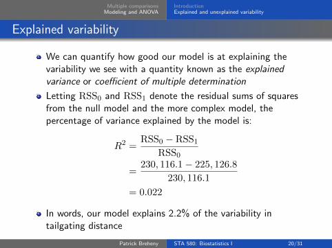
Explained variability
We can quantify how good our model is at explaining thevariability we see with a quantity known as the explainedvariance or coefficient of multiple determination
Letting RSS0 and RSS1 denote the residual sums of squaresfrom the null model and the more complex model, thepercentage of variance explained by the model is:
R2 =RSS0 − RSS1
RSS0
=230, 116.1 − 225, 126.8
230, 116.1
= 0.022
In words, our model explains 2.2% of the variability intailgating distance
Patrick Breheny STA 580: Biostatistics I 20/31
Multiple comparisonsModeling and ANOVA
IntroductionExplained and unexplained variability
Complex models always fit better
Still, the more complex model has a lower residual sum ofsquares; it must be a better model then, right?
Not necessarily; the more complex model will always have alower residual sum of squares
The reason is that, even if the population means are exactlythe same for the four groups, the sample means will beslightly different
Thus, a more complex model that allows the modeled meansin each group to be different will always fit the observed databetter
But that doesn’t mean it would explain the variability of futureobservations any better (this concept is called overfitting)
Patrick Breheny STA 580: Biostatistics I 21/31

Multiple comparisonsModeling and ANOVA
IntroductionExplained and unexplained variability
ANOVA
The real question is whether this reduction in the residual sumof squares is larger than what you would expect by chancealone
This type of model – one where we have several differentgroups and are interested in whether the groups have differentmeans – is called an analysis of variance model, or ANOVA forshort
The meaning of the name is historical, as this was the firsttype of model to hit on the idea of looking at explainedvariability (variance) to test hypotheses
Today, however, many different types of models use this sameidea to conduct hypothesis tests
Patrick Breheny STA 580: Biostatistics I 22/31

Multiple comparisonsModeling and ANOVA
IntroductionExplained and unexplained variability
Parameters
To answer the question of whether the reduction in RSS issignificant, we need to keep track of the number ofparameters in a model
For example, the null model had one parameter: the commonmean
In contrast, the more complex model had four parameters: theseparate means of the four groups
Let’s let d denote the number of parameters, so d0 = 1 andd1 = 4
Patrick Breheny STA 580: Biostatistics I 23/31
Multiple comparisonsModeling and ANOVA
IntroductionExplained and unexplained variability
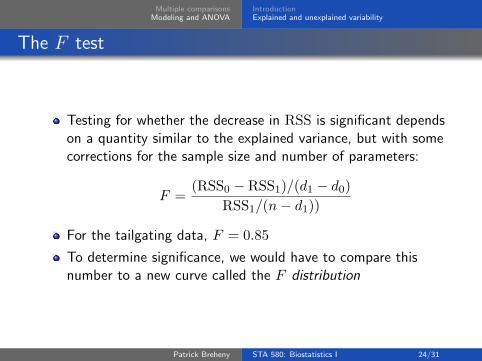
The F test
Testing for whether the decrease in RSS is significant dependson a quantity similar to the explained variance, but with somecorrections for the sample size and number of parameters:
F =(RSS0 − RSS1)/(d1 − d0)
RSS1/(n− d1))
For the tailgating data, F = 0.85
To determine significance, we would have to compare thisnumber to a new curve called the F distribution
Patrick Breheny STA 580: Biostatistics I 24/31

Multiple comparisonsModeling and ANOVA
IntroductionExplained and unexplained variability
F distribution
0 1 2 3 4 5
0.0
0.1
0.2
0.3
0.4
0.5
0.6
0.7
F
Den
sity
p=0.47
Patrick Breheny STA 580: Biostatistics I 25/31
Multiple comparisonsModeling and ANOVA
IntroductionExplained and unexplained variability
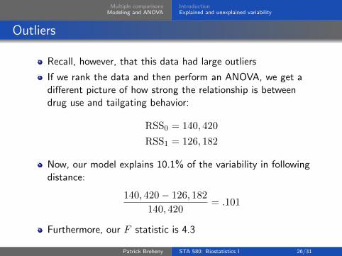
Outliers
Recall, however, that this data had large outliers
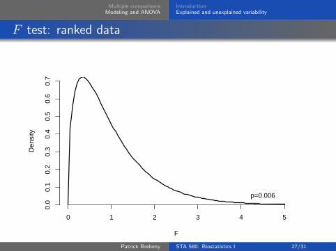
If we rank the data and then perform an ANOVA, we get adifferent picture of how strong the relationship is betweendrug use and tailgating behavior:
RSS0 = 140, 420
RSS1 = 126, 182
Now, our model explains 10.1% of the variability in followingdistance:
140, 420 − 126, 182
140, 420= .101
Furthermore, our F statistic is 4.3
Patrick Breheny STA 580: Biostatistics I 26/31
Multiple comparisonsModeling and ANOVA
IntroductionExplained and unexplained variability
F test: ranked data
0 1 2 3 4 5
0.0
0.1
0.2
0.3
0.4
0.5
0.6
0.7
F
Den
sity
p=0.006
Patrick Breheny STA 580: Biostatistics I 27/31

Multiple comparisonsModeling and ANOVA
IntroductionExplained and unexplained variability
Means and CIs: Original
020
4060
80
Dis
tanc
e
ALC MDMA NODRUG THC
Patrick Breheny STA 580: Biostatistics I 28/31

Multiple comparisonsModeling and ANOVA
IntroductionExplained and unexplained variability
Means and CIs: Ranked
020
4060
8010
0
rank
(Dis
tanc
e)
ALC MDMA NODRUG THC
Patrick Breheny STA 580: Biostatistics I 29/31
Multiple comparisonsModeling and ANOVA
IntroductionExplained and unexplained variability
ANOVA for two groups?
We have seen that ANOVA models can be used to testwhether or not three or more groups have the same mean
Could we have used models to carry out two-groupcomparisons?
Of course; however, comparing the amount of variabilityexplained by a two-mean vs. a one-mean model producesexactly the same test as Student’s t-test
Patrick Breheny STA 580: Biostatistics I 30/31
Multiple comparisonsModeling and ANOVA
IntroductionExplained and unexplained variability
Other uses for statistical models
Statistical models have uses far beyond comparing multiplegroups, such as adjusting for the effects of confoundingvariables, predicting future outcomes, and studying therelationships between multiple variables
Statistical modeling is a huge topic, and we are barelyskimming the surface today
Statistical models are the focus of the next course in thissequence, Biostatistics II (CPH 630)
Patrick Breheny STA 580: Biostatistics I 31/31


