Understand how ‘analysis of variance’(ANOVA) can

be used to test for the equality of three or more

population means.

Understand and use the terms like ‘response

variable’, ‘a factor’ and ‘a treatment’ in the analysis

of variance.

Learn how to summarize F-ratio in the form of an

ANOVA table.

Objectives

ANOVA

The null hypothesis states that there is no significant difference among population

mean, that is, H0 : μ1 = μ2 . However, there may be situations where more than two

populations are involved and we need to test the significance of differences between

three or more sample means. We also need to test the null hypothesis that three or

more populations from which independent samples are drawn have equal (or

homogeneous) means against the alternative hypothesis that population means are

not all equal. Let μ1 = μ2 =…….. =μr be the mean value for population 1, 2, . . ., r

respectively. Then from sample data we intend to test the following hypotheses:

H0 : μ1 = μ2 =…….. =μr

and H1 : Not all μj are equal ( j = 1, 2, . . ., r)

In other words, the null and alternative hypotheses of population means imply that

the null hypothesis should be rejected if any of the r sample means is different from

the others.

Examples:

• Effectiveness of different promotional devices in terms of sales

• Quality of a product produced by different manufacturers in

terms of attribute

• Production volumes in different shifts in a factory

• Yield from plots of land due to varieties of seeds, fertilizers and

cultivation methods

• Effectiveness of different techniques of improving employees

morale.

The following are few terms that will be used during discussion on

analysis of variance:

A sampling plan or experimental design is the way that a

sample is selected from the population under study and

determines the amount of information in the sample.

An experimental unit is the object on which a measurement

or measurements is taken. Any experimental conditions

imposed on an experimental unit provides effect on the

response.

A factor or criterion is an independent variable whose values

are controlled and varied by the researcher.

A level is the intensity setting of a factor.

A treatment or population is a specific combination of factor

levels.

The response is the dependent variable being measured by

the researcher.

Examples 1: For a production volume in three shifts in a factory, there are

two variables—days of the week and the volume of production in each

shift. If one of the objectives is to determine whether mean production

volume is the same during days of the week, then the dependence (or

response) variable of interest, is the mean production volume. The

variables that are related to a response variable are called factors, that is,

a day of the week is the independent variable and the value assumed by a

factor in an experiment is called a level. The combinations of levels of the

factors for which the response will be observed are called treatments, i.e.

days of the week. These treatments define the populations or samples

which are differentiated in terms of production volume and we may need

to compare them with each other.

Examples in Managerial Aspects:

Example 2: A tyre manufacturing company plans to conduct a tyre

quality study in which quality is the independent variable called factor

or criterion and the treatment levels or classifications are low, medium

and high quality. The dependent (or response) variable might be the

number of kilometers driven before the tyre is rejected for use.

Example 3: A study of daily sales volumes may taken by using a

completely randomized design with demographic setting as the

independent variable. A treatment levels or classification would be

inner-city stores, stores in metro cities, stores in state capitals, stores in

small towns, etc. The dependent variables would be sales in rupees.

The following assumptions are required for analysis of variance:

1. Each population under study is normally distributed with a

mean μr that may or may not be equal but with equal variance

2. Each sample is drawn randomly and is independent of other

samples.

2

r

Approach of ANOVA

• One-way classification

• Two-way classification

• Direct method

• Short-cut method

• Coding method

Testing Equality of Population Means: One-way

ClassificationSuppose our aim is to make inferences about r population means μ1,μ2, . .

. μr based on independent random samples of size n1, n2, . . ., nr, from

normal populations with a common variances σ2. That is, each of the

normal population has same shape but their locations might be different.

The null hypothesis to be tested is stated as:

H0 : μ1 = μ 2 = . . . = μ r

H1 : Not all μ j ( j = 1, 2, . . ., r) are equal

Let nj = size of the jth sample ( j = 1, 2,...., r)

n = total number of observations in all samples combined

(i.e. n = n1 + n2 + . . . + nr)

xij = the ith observation value within the sample from jth population

The observations values obtained for r independent samples based on one-

criterion classification can be arranged as shown in the following table.

One-Criterion Classification of Data

k

i

r

jij

r

jj

k

iiji

r

jj

k

iijj

xn

xrk

xxk

x

TTxT

1 111

11

111

where

The values of xi are called sample means and is the grand mean

of all observations (or measurements) in all the samples.

Since there are k rows and r columns in table, therefore, total

number of observations are rk = n, provided each row has equal

number of observations. But, if the number of observations in each

row varies, then the total number of observations is n1 + n2 + . . . +

nr = n.

x

Steps for Testing Null Hypothesis

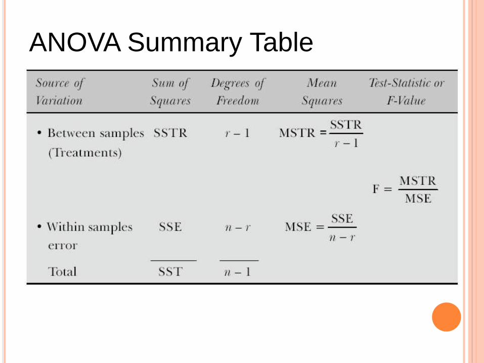
ANOVA Summary Table

Short-Cut Method

Inferences About Population (Treatment)

Means

Two-way Analysis of Variance

Analysis of variance in which two criteria (or variables) are used to analyze the

difference between more than two population means.

The two-way analysis of variance can be used to

explore one criterion (or factor) of interest to partition the sample data so

as to remove the unaccountable variation, and arriving at a true

conclusion.

investigate two criteria (factors) of interest for testing the difference

between sample means.

consider any interaction between two variables.

In two-way analysis of variance we are introducing another term called ‘blocking variable’ to

remove the undesirable accountable variation. A block variable is the variable that the

researcher wants to control but is not the treatment variable of interest. The term ‘blocking’

refers to block of land and comes from agricultural origin. The ‘block’ of land might make some

difference in the study of growth pattern of varieties of seeds for a given type of land. R. A.

Fisher designated several different plots of land as blocks, which he controlled as a second

variable. Each of the seed varieties were planted on each of the blocks. The main aim of his

study was to compare the seed varieties (independent variable). He wanted only to control the

difference in plots of land (blocking variable). ‘Blocking’ is an extension of the idea of pairing

observations in hypothesis testing. Blocking provides the opportunity for one-to-one

comparison of prices, where any observed difference cannot be due to difference among

blocking variables.

The partitioning of total variation in the sample data is shown below:

General ANOVA Table for Two-way

Classification

As stated above, total variation consists of three parts: (i) variation between

columns, SSTR; (ii) variation between rows, SSR; and (iii) actual variation due

to random error, SSE. That is

SST = SSTR + (SSR + SSE)

The degrees of freedom associated with SST are cr – 1, where c and r are the

number of columns and rows, respectively

Degrees of freedom between columns = c – 1

Degrees of freedom between rows = r – 1

Degrees of freedom for residual error = (c – 1) (r – 1) = N – n – c + 1

The test-statistic F for analysis of variance is given by

Ftreatment = MSTR/MSE; MSTR > MSE or MSE/MSTR; MSE > MSTR

Fblocks = MSR/MSE; MSR > MSE or MSE/MSR; MSE > MSR

Decision rule

If Fcal < Ftable, accept null hypothesis H0

Otherwise reject H0