Anticipation of Monetary Policy and Open Market Operations · Anticipation of Monetary Policy and...

Anticipation of Monetary Policyand Open Market Operations∗

Seth B. Carpentera and Selva Demiralpb

aFederal Reserve BoardbDepartment of Economics, Koc University

Central banking transparency is now a topic of great inter-est, but its impact on the implementation of monetary policyhas not been studied. This paper documents that anticipatedchanges in the target federal funds rate complicate open mar-ket operations. We provide theoretical and empirical evidenceon the behavior of banks and the Open Market Trading Desk.We find a significant shift in demand for funds ahead ofexpected target rate changes and that the Desk only incom-pletely accommodates this shift in demand. This anticipationeffect, however, does not materially affect other markets.

JEL Codes: E5, E52, E58.

1. Introduction

Through time, the Federal Reserve has been perceived as becomingmore open and transparent. For example, explicit announcements ofchanges in the target federal funds rate began in 1994. With pre-dictable changes in monetary policy, financial markets move beforethe Federal Reserve, not just in reaction to it. Lange, Sack, andWhitesell (2003) find empirical evidence of an anticipation effect in

∗The views expressed are those of the authors and do not necessarily reflectthose of the Board of Governors, the Federal Reserve System, or other membersof the staff. We thank Kristin van Gaasbeck, James Hamilton, Mark Gertler,seminar participants at the Board of Governors of the Federal Reserve System,and staff at the Open Market Trading Desk at the Federal Reserve Bank of NewYork for their invaluable comments. Author contact: Carpenter: Mail Stop 59,20th and C Street NW, Washington, DC 20551; e-mail: [email protected]: Department of Economics, Koc University, Istanbul, Turkey; e-mail:[email protected].

25

26 International Journal of Central Banking June 2006

the market for Treasury securities in the months prior to changes inmonetary policy.

In this paper, we investigate whether a similar type of anticipa-tion effect exists in the federal funds market, the overnight loans ofbalances on deposit at the Federal Reserve. The supply of balancesin this market is influenced by the Open Market Trading Desk atthe Federal Reserve Bank of New York in order to push tradingin the market toward the target rate determined by the FederalOpen Market Committee (FOMC). On the one hand, because thismarket is the most directly affected by monetary policy, one mightthink that an anticipation effect would more likely be present in thismarket. On the other hand, supply is controlled by the Desk to off-set any rate pressures. As a result, deviations from the target couldreflect constraints that the Desk faces in accomplishing its goal. Pre-dictable changes in the target rate could therefore have implicationsfor the conduct of open market operations. In addition, an antici-pation effect is related to, but distinct from, changes in the fundsrate that are a result of an announcement by the Federal Reserve.Demiralp and Jorda (2002) and Hanes (2005) analyze these so-calledopen-mouth operations by looking at the movement of the funds rateafter a target change announcement, not prior to it.

In this paper, we look into why an anticipation effect in thefederal funds market exists and what the broader implications are.We present evidence that the federal funds rate tends to move in thedirection of an anticipated change in policy prior to that change. Weestimate econometric models of the federal funds market at a dailyfrequency in the spirit of Hamilton (1997, 1998) and Carpenter andDemiralp (forthcoming) to filter out the systematic variation in thefunds rate and to estimate the movement that is attributable solelyto the anticipation effect. Turning from the price side to the quan-tity side, we present results on the supply of reserve balances thatsuggest that the Desk increases the supply of balances in response tothe anticipation effect. The fact that federal funds trade away fromthe current target, however, suggests that the change in supply is notsufficient to achieve the target. Indeed, in its annual report for 2004,the Desk acknowledged that it has attempted to offset only par-tially a shift in demand, because fully offsetting the demand couldlead to unwanted volatility in the federal funds market. We attemptto assess this rationale based on our results.

Vol. 2 No. 2 Anticipation of Monetary Policy 27

Because the anticipation effect is the result of a shift in demand,we present an optimizing, dynamic programming model of a repre-sentative bank’s demand for daily reserve balances to explain theshift in demand.1 The model indicates that demand is shifted by afinite amount, suggesting that a full offset to the shift in demand ispossible. First, we discuss the open market operations that would benecessary to counteract this effect. We conclude that it is possiblethat fully offsetting the rise in rates before fully anticipated movescould result in a substantial decline in the funds rate relative to thetarget following the FOMC meeting in question. We then documentthat over the period studied, there has been no significant increasein volatility surrounding the meetings. Lastly, we show that therehas been little spillover from the funds market to other financialmarkets.

2. Data and Econometric Evidence

To examine the anticipation effect, we turn to the market for FederalReserve balances. Reserve requirements, based on banks’ customers’reservable deposits, are satisfied either with vault cash or with bal-ances at the Federal Reserve. These balances are called requiredreserve balances. In addition, banks may contract with the FederalReserve to hold more balances to facilitate the clearing of transac-tions through their accounts. These balances are called contractualclearing balances. Holdings of required balances—the sum of requiredreserve balances and contractual clearing balances—are averagedover a fourteen-day period called a maintenance period. Any bal-ances held beyond the required level are called excess balances. Themarket for balances is discussed in more detail in section 3.

We use business-day data from February 1994 through July 2005.The starting date reflects the Federal Reserve’s adoption of a policyof announcing changes in the target federal funds rate. We spec-ify an equation with the deviation of the effective federal funds ratefrom its target as the dependent variable, and we specify an equationwith the level of daily excess reserves as the dependent variable. Foreach equation, we include a lagged dependent variable to capture the

1In this paper we frequently use the generic word “bank” to represent depos-itory and other institutions with accounts at the Federal Reserve.


autoregressive behavior. We also include dummy variables for eachday of the maintenance period to control for systematic variationin the variables; Carpenter and Demiralp (forthcoming) documentan intra-maintenance-period pattern to the federal funds rate. Weinclude the level of cumulative reserve balances to control for thefact that demand for balances has a maintenance-period-frequencycomponent as well as a daily-frequency component. In an extremeexample, on the last day of a maintenance period, one would expectdemand to be lighter than usual if banks had already satisfied theirbalance requirements for the period. We include the error for thedaily forecast of balances made by the Federal Reserve. Hamilton(1998) and Carpenter and Demiralp (forthcoming) use this vari-able to measure the liquidity effect in the funds market. We useit here to capture deviations in price and quantity that are dueto unintentional changes in reserve balances. As shown later, ourresults for the liquidity effect are broadly consistent with previouswork.

We also include separate dummy variables for “special pressuredays”—specifically, the day after a holiday; quarter end; year end;first of the month; fifteenth of the month; month end; and settle-ment of Treasury two-, three-, five-, and ten-year notes, includingTreasury inflation-protected securities.2 These are days of increasedpayment flows through banks’ reserve accounts and, as a result, rep-resent days of increased uncertainty. Increased uncertainty shouldbe associated with a greater demand for balances to avoid an over-draft. Finally, for the excess balances equation, we include carryover,broken down by bank size. Everything else remaining the same, ahigher level of balances carried over from the previous maintenanceperiod should induce banks to hold lower balances in the currentmaintenance period.

While the regressions include the control variables as well as thevariables of interest, to ease exposition, we present the coefficientson these control variables first in table 1 before presenting the restof the results from the model. Looking at the dummies for the days

2We exclude Treasury bill auctions, as these are regular weekly auctions andare thus captured by our daily dummy variables. The exceptions to this wouldbe the handful of occasions when bill auctions were delayed due to debt limitconstraints.


Table 1. Control Variables

Sample Period: January 26, 1994–July 13, 2005*

(Deviation fromTarget)t (Daily ER)t

Variable Coeff. s.e. Coeff. s.e.

Lagged Dependent Variable 0.27 0.047 0.27 0.026

DFirst Thursday −0.00082 0.015 0.65 0.28

DFirst Friday −0.058 0.016 0.056 0.26

DFirst Monday 0.0033 0.016 1.53 0.22

DFirst Tuesday −0.049 0.015 0.93 0.23

DFirst Wednesday −0.032 0.015 0.98 0.23

DSecond Thursday 0.00030 0.015 1.54 0.23

DSecond Friday −0.064 0.015 1.66 0.22

DSecond Monday 0.026 0.016 4.13 0.27

DSecond Tuesday −0.040 0.018 4.22 0.41

DSecond Wednesday 0.12 0.031 9.63 1.23

Cumulative ER× DFirst Friday −0.011 0.0030 −0.082 0.069

Cumulative ER× DFirst Monday −0.0083 0.0048 −0.089 0.069

Cumulative ER× DFirst Tuesday −0.0082 0.0028 −0.35 0.073

Cumulative ER× DFirst Wednesday −0.016 0.0041 −0.37 0.072

Cumulative ER× DSecond Thursday −0.017 0.0038 −0.70 0.074

Cumulative ER× DSecond Friday −0.013 0.0049 −1.0039 0.093

Cumulative ER× DSecond Monday −0.016 0.010 −1.79 0.24

Cumulative ER× DSecond Tuesday −0.040 0.011 −2.058 0.47

Cumulative ER× DSecond Wednesday −0.090 0.024 −4.11 1.22

(Forecast Miss)t −0.0095 0.0035 0.79 0.038

DMonth End 0.027 0.034 2.45 0.26

DMonth Start 0.012 0.021 1.60 0.22

DQuarter End 0.28 0.0764 4.27 0.41

DQuarter Start 0.17 0.081 2.54 0.42

DYear End −0.45 0.17 5.047 1.21

DYear Start 0.25 0.11 1.94 0.81

(continued)


Table 1 (continued). Control Variables




DMid-Month 0.09 0.012 2.31 0.20

DDay Before Holiday −0.02 0.017 0.10 0.19

DDay After Holiday −0.06 0.077 1.73 0.21

DTreasury 2 0.11 0.041 −0.85 0.36

DTreasury 3 0.065 0.032 −0.51 0.41

DTreasury 5 0.098 0.045 1.47 0.39

DTreasury 10 −0.045 0.016 −0.33 0.39

(Required Operating Balances)t 0.00070 0.00059 −0.042 0.0085

Target 0.0014 0.0012 −0.13 0.023

(Carry-in Large)t — — −0.51 0.43

(Carry-in Other)t — — 4.69 1.85

(Carry-in Large)t × Anticipated ∆ — — −5.17 12.0080× DOne Day Before a Tightening

(Carry-in Large)t × Anticipated ∆ — — −2.931 10.021× DOne Day Before an Easing

Note: Tables 1 and 2 report the results from the same regression but split the variablesinto two groups for exposition.*Data for 2001 exclude September 11 through September 19.

of the maintenance period, we note that both Fridays have negativeand statistically significant coefficients in the federal funds equation,as shown in the second and third columns. These results suggest thatthe funds rate consistently trades soft to the target on Fridays andindicate that the Desk typically provides more reserves on Fridaysthan are demanded at the target. Also of note is that the fundsrate systematically trades firm to the target on the last day of themaintenance period. From the excess balances equation, shown inthe last two columns, we can see that excess balances tend to startoff low early in the period and gradually rise, peaking on settlementWednesday.


Looking at the coefficients on cumulative excess, although manyof the coefficients in the federal funds equation are statistically sig-nificant, they are only economically significant on the last two days,where an extra $1 billion of cumulative excess is associated with 4and 9 basis points of softness, respectively. The negative coefficientsin the excess balances equation suggest that the Desk recognizesthe pressure that cumulative excess places on banks’ demand forbalances and works to offset the effect.

The carryover variable is negative for the large banks, indicatingthat these institutions act with the motivation to maximize prof-its and use their reserves efficiently. The coefficient is positive forsmall banks, confirming our understanding that these institutions donot closely manage their reserve positions. In order to test whetherthe banks boost their balances in the maintenance period before ananticipated rate hike in order to carry over the surplus, we inter-act lagged carryover balances with anticipated policy changes onthe day before a target change for large banks. The coefficients areinsignificant.

The coefficient on the forecast miss is consistent with results inCarpenter and Demiralp (forthcoming) for the funds rate equation.Essentially, this coefficient says that a $1 billion change in reservebalances changes the federal funds rate about 1 basis point. For theexcess balances equation, the coefficient is slightly (but statisticallysignificantly) less than unity. Hamilton (1997) suggests that theseexogenous changes in reserve balances are partially offset by borrow-ing from the discount window, an interpretation consistent with acoefficient below 1. The other variables have similar, logical interpre-tations. On balance, these control variables should allow us to focusexclusively on the anticipation effect, feeling confident that we haveaccounted for other systematic variation in the dependent variables.

2.1 Measuring Anticipation

Figure 1 shows the deviation of the effective federal funds rate fromthe target rate on days leading up to policy changes at FOMC meet-ings over the period 1994 to 2004. As can be seen, on days prior toincreases in the target, the funds rate was on average above thetarget rate, and on days prior to decreases in the target, the fundsrate was below the target. While this evidence is suggestive, it does


Figure 1. Federal Funds Rate Deviations from TargetSurrounding a Target Change (1994–2004)

*Data for 2001 exclude September 11 through September 19.

not control for whether or not the change in the target rate wasexpected—the crux of the anticipation effect.

To measure the degree of anticipation of changes in the targetrate, we use a technique that generalizes the methodology proposedby Kuttner (2001) to measure expectations of the Federal Reserve’spolicy actions based on the price of federal funds futures contracts.3

The key idea is that the spot-month rate for federal funds futurescontracts on a particular day t reflects the expected average fundsrate for that month, conditional on the information prevailing up tothat date.4 Based on this fact and knowing that the effective funds

3One ironic implication of the present paper is that a systematic anticipationeffect should tend to get priced into futures contracts. As a result, the method forinferring anticipated changes is likely biased. Preliminary investigation of the phe-nomenon suggests that the bias is likely small, but future research should strive tomake the estimation precise. In any event, this bias implies that we will understateany anticipation effect we find, so our general results should be unaffected.

4Naturally, this measure presumes that market participants are aware of thetarget and can observe the changes. If the market participants were unaware thatthe target had changed, expectations would not necessarily reflect the changesin the policy instrument.


rate as a monthly average is very close to the target rate (typicallywithin a few basis points), the spot-month futures rate on any dayk prior to a target change that is expected to occur on day t can beexpressed as

Spot Ratek =[(Nb × ρt−1) + (Na × Ek(ρt)]

N+ µk, k < t, (1)

where ρt is the target funds rate on day t, Ek is the expectationsoperator based on information as of day k, and µk is a term that mayrepresent the risk premium or day-of-month effects in the futuresmarket. In an efficient market with risk-neutral investors, this termwould be zero. Nb is the number of days before a target change, Na

is the number of days after a target change, and hence N = Nb +Na

is the total number of days in a given month.Assuming that the target change occurs on day t, the spot rate

on day t is given by

Spot Ratet =[(Nb × ρt−1) + (Na × ρt)]

N+ µt. (2)

The difference between the spot-month rates prior to and afterthe target change—i.e., equation (2) − equation (1)—gives us thepolicy surprise as of day k:

Spot Ratet − Spot Ratek

= Φ [ρt − Ek(ρt)]︸︷︷︸Unanticipated target change as of day k

, where Φ =(

Na

N

). (3)

Equation (3) is used to compute the policy surprise on any dayk prior to a target change that takes place on day t (i.e., k < t),except for two cases:

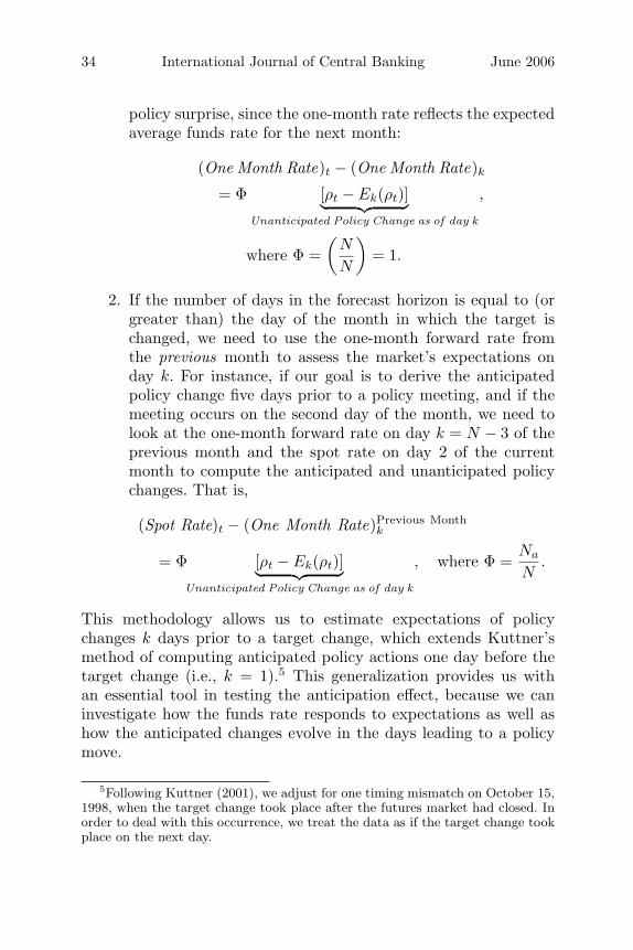
1. Kuttner (2001) notes that the day-t targeting error and therevisions in the expectation of future targeting errors maybe nontrivial at the end of the month. Consequently, if atarget change occurs in the last three days of the month, thedifference in one-month forward rates is used to derive the


policy surprise, since the one-month rate reflects the expectedaverage funds rate for the next month:

(One Month Rate)t − (One Month Rate)k

= Φ [ρt − Ek(ρt)]︸︷︷︸Unanticipated Policy Change as of day k

,

where Φ =(

N

N

)= 1.

2. If the number of days in the forecast horizon is equal to (orgreater than) the day of the month in which the target ischanged, we need to use the one-month forward rate fromthe previous month to assess the market’s expectations onday k. For instance, if our goal is to derive the anticipatedpolicy change five days prior to a policy meeting, and if themeeting occurs on the second day of the month, we need tolook at the one-month forward rate on day k = N − 3 of theprevious month and the spot rate on day 2 of the currentmonth to compute the anticipated and unanticipated policychanges. That is,

(Spot Rate)t − (One Month Rate)Previous Monthk

= Φ [ρt − Ek(ρt)]︸︷︷︸Unanticipated Policy Change as of day k

, where Φ =Na

N.

This methodology allows us to estimate expectations of policychanges k days prior to a target change, which extends Kuttner’smethod of computing anticipated policy actions one day before thetarget change (i.e., k = 1).5 This generalization provides us withan essential tool in testing the anticipation effect, because we caninvestigate how the funds rate responds to expectations as well ashow the anticipated changes evolve in the days leading to a policymove.

5Following Kuttner (2001), we adjust for one timing mismatch on October 15,1998, when the target change took place after the futures market had closed. Inorder to deal with this occurrence, we treat the data as if the target change tookplace on the next day.


2.2 Estimating the Anticipation Effect

Before we present the regression coefficients associated with theanticipation effect, it is informative to take a look at how the accu-racy of policy expectations has evolved in time. Figure 2 displays thecomponents of target changes that are unanticipated by the mar-ket for policy tightenings and easings, respectively.6 Consistent withthe improvements in the transparency of monetary policy actions,the component of target changes that surprised market participantsdeclined gradually over time both for policy tightenings and policyeasings.

As noted above, we interacted the expected change in the federalfunds rate with dummy variables for one through nine days before apolicy change. To avoid conditioning our estimation on whether ornot there was a policy change, a fact that is only known ex post,7 wefocus exclusively on anticipation of policy changes that took placeat FOMC meetings.8 Of course, during our sample period, therewere intermeeting policy changes, but these moves were all surprises,and we do not believe that banks planned in advance for them. Wedo, however, want to allow for an asymmetry between an expectedincrease and an expected decrease. We interact the expected changein the funds rate with a dummy variable that denotes an upcomingFOMC meeting. To allow for the asymmetry, we create one dummyfor meetings where there was either no change or an increase inthe funds rate and another for meetings where there was either nochange or a decrease in the funds rate. We assume, therefore, that thesign of an impending change in the target rate change is known bybanks—an assumption we view as entirely plausible. Because some

6Unanticipated change is computed as the difference between the actual sizeof a target change and the anticipated change.

7We thank Jim Hamilton for pointing out our previous error in conditioningon information only knowable ex post.

8Prior to 1998, during the period of contemporaneous reserve accounting,reserve requirements and contractual clearing balances were calculated over acomputation period that overlapped with all but the last two days of the mainte-nance period over which the requirements were to be satisfied. Since 1998, com-putation periods have ended prior to the beginning of the maintenance period.We interacted dummy variables for the lagged-accounting period with the antici-pation variable to test whether or not this structural shift affects our results. Wefail to reject that the coefficients are jointly equal to zero.


Figure 2. Unanticipated Target Changes on the Daybefore a Policy Action

of the observations that are multiple days prior to a policy move arein a previous maintenance period, we include in our estimation onlythose anticipations that are in the same maintenance period, withinwhich the motivation to clear arbitrage opportunities is dominant.


Table 2. Anticipation Effect



Anticipated ∆ × DNine Days Before a Tightening 0.055 0.054 1.33 0.88

Anticipated ∆ × DEight Days Before a Tightening 0.056 0.058 0.050 0.57

Anticipated ∆ × DSeven Days Before a Tightening 0.014 0.044 1.23 0.58

Anticipated ∆ × DSix Days Before a Tightening 0.057 0.043 0.41 0.47

Anticipated ∆ × DFive Days Before a Tightening 0.028 0.044 0.31 0.34

Anticipated ∆ × DFour Days Before a Tightening 0.12 0.055 0.68 0.40

Anticipated ∆ × DThree Days Before a Tightening 0.29 0.060 1.26 0.34

Anticipated ∆ × DTwo Days Before a Tightening 0.37 0.052 1.87 0.34

Anticipated ∆ × DOne Day Before a Tightening 0.46 0.067 1.17 0.44

Anticipated ∆ × DNine Days Before an Easing 0.078 0.083 1.45 1.0089

Anticipated ∆ × DEight Days Before an Easing 0.11 0.13 0.38 0.53

Anticipated ∆ × DSeven Days Before an Easing −0.066 0.19 −0.37 0.57

Anticipated ∆ × DSix Days Before an Easing −0.11 0.11 −0.30 0.48

Anticipated ∆ × DFive Days Before an Easing −0.0078 0.049 0.26 0.57

Anticipated ∆ × DFour Days Before an Easing 0.078 0.058 −0.57 0.46

Anticipated ∆ × DThree Days Before an Easing 0.017 0.059 −0.20 0.46

Anticipated ∆ × DTwo Days Before an Easing 0.18 0.11 −0.34 0.56

Anticipated ∆ × DOne Day Before an Easing 0.23 0.076 −0.055 0.74

DDay of a Tightening −0.18 0.048 0.42 0.57

DDay of an Easing 0.089 0.029 −0.38 0.36

DDay of a Tightening × Unanticipated ∆ −0.50 0.62 −5.40 7.60

DDay of an Easing × Unanticipated ∆ 0.43 0.56 5.22 2.97

Notes: Tables 1 and 2 report the results from the same regression but split the vari-ables into two groups. For Daily ER regressions, the anticipated change variable isreplaced with a dummy variable where |Anticipated ∆| > 0.125.

The results shown are from the regression that had the controlvariables reported in table 1. As shown in the second and thirdcolumns of table 2, the results for the federal funds rate equationindicate a statistically significant anticipation effect in the fundsmarket only for four days prior to a tightening and for two days prior


to an easing.9 The coefficients suggest that the funds rate moves inthe direction of the anticipated change, but not fully. Prior to antic-ipated tightenings, the funds rate moves almost halfway—or about121/2 basis points for an anticipated 25-basis-point policy move—tothe anticipated new target on the day before the policy change andis elevated as many as three days prior. For anticipated easings, theeffect is much more muted, although it is still statistically signif-icant. This asymmetric effect will be confirmed in our theoreticalmodel presented below. Because requirements are satisfied over atwo-week period, there is an option value to waiting until the latterpart of the period to satisfy these requirements. Given this pattern,which is reflected both in the data and in our model, there is lessscope for banks to react to an anticipated easing by lowering bal-ances further to take advantage of lower expected rates later in theperiod. Doing so would increase the probability of a costly overnightoverdraft, and so the anticipation effect in this case is attenuated.For anticipated policy easings, the funds rate appears to move lessthan one-fourth of the way to the anticipated new target, or about 6basis points for a 25-basis-point reduction in the target funds rate.

We do find some evidence that the Desk accommodates theincrease in demand for reserve balances prior to an anticipated pol-icy tightening—as indicated by the positive, statistically significantcoefficients up to four days prior to a tightening, shown in the lasttwo columns. Those results imply that over the four days before afully anticipated increase in the target federal funds rate, the Deskprovides between $.75 and $1.75 billion more in excess reserve eachday than would be typical, holding all other things constant, fora total of about $5 billion. Taking the results of the two equationstogether, however, we can infer that the increase in supply is not suf-ficient to fully offset the increased demand; the evidence is the fundsrate trading firm to the target despite an increased provision of bal-ances. These results imply that the Desk leans against the firmnessbut does not fully counteract it. Similarly, prior to anticipated policy

9For the excess balances equation, we replace the expected change with adummy variable that equals 1 if the expected change is greater than 121/2 basispoints; that is to say, better than even odds of at least a 25-basis-point change.This substitution is made because banks must decide if they think a change iscoming or not, rather than acting on the size of the change, in order to shiftbalances.


easings, the Desk does not drain sufficient balances to offset fully thesoftness in the market, likely in an effort to avoid leaving the Systemwith insufficient balances.

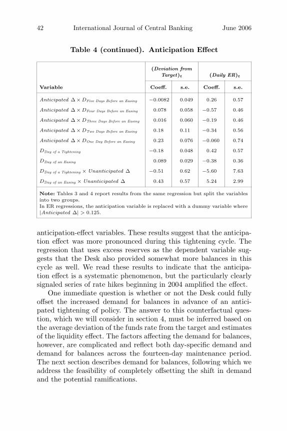
The tightening episode that began in June 2004 has been char-acterized as particularly well anticipated and predictable. As anextension, we test to see if the anticipation effect is different in thisrecent episode. Tables 3 and 4 present the same regressions but withdummy variables for the 2004 tightening episode interacted with our

Table 3. Control Variables




Lagged Dependent Variable 0.27 0.047 0.27 0.026

DFirst Thursday −0.0033 0.016 0.59 0.28

DFirst Friday −0.061 0.016 0.0040 0.26

DFirst Monday 0.0011 0.016 1.46 0.23

DFirst Tuesday −0.051 0.015 0.87 0.24

DFirst Wednesday −0.034 0.015 0.94 0.23

DSecond Thursday −0.0014 0.015 1.49 0.23

DSecond Friday −0.066 0.015 1.63 0.23

DSecond Monday 0.024 0.016 4.11 0.27

DSecond Tuesday −0.041 0.018 4.18 0.41

DSecond Wednesday 0.12 0.031 9.58 1.23

Cumulative ER× DFirst Friday −0.011 0.0030 −0.084 0.069

Cumulative ER× DFirst Monday −0.0087 0.0048 −0.10 0.070

Cumulative ER× DFirst Tuesday −0.0083 0.0028 −0.35 0.073

Cumulative ER× DFirst Wednesday −0.016 0.0041 −0.37 0.072

Cumulative ER× DSecond Thursday −0.018 0.0038 −0.70 0.073

Cumulative ER× DSecond Friday −0.013 0.0050 −1.0070 0.093

(continued)


Table 3 (continued). Control Variables




Cumulative ER× DSecond Monday −0.016 0.010 −1.80 0.25

Cumulative ER× DSecond Tuesday −0.040 0.011 −2.07 0.48

Cumulative ER× DSecondWednesday −0.090 0.024 −4.10 1.22

(Forecast Miss)t −0.0094 0.0035 0.79 0.038

DMonth End 0.025 0.035 2.45 0.26

DMonth Start 0.013 0.021 1.58 0.22

DQuarter End 0.28 0.077 4.27 0.41

DQuarter Start 0.17 0.081 2.55 0.43

DYear End −0.45 0.17 5.051 1.21

DYear Start 0.25 0.11 2.017 0.76

DMid-Month 0.091 0.012 2.33 0.20

DDay Before Holiday −0.020 0.017 0.11 0.19

DDay After Holiday −0.060 0.077 1.74 0.21

DTreasury 2 0.11 0.041 −0.89 0.36

DTreasury 3 0.067 0.032 −.44 0.40

DTreasury 5 0.098 0.045 1.52 0.39

DTreasury 10 −0.044 0.016 −.34 0.39

(Required Operating Balances)t 0.00072 0.00057 −.041 0.0085

Target 0.0018 0.0013 −.13 0.024

(Carry-in Large)t — — −.54 0.43

(Carry-in Other)t — — 4.67 1.85

(Carry-in Large)t × Anticipated ∆ — — −.58 9.70× DOne Day Before a Tightening

(Carry-in Large)t × Anticipated ∆ — — −.74 10.070× DOne Day Before an Easing

Note: Tables 3 and 4 report results from the same regression but split the variablesinto two groups.*Data for 2001 exclude September 11 through September 19.


Table 4. Anticipation Effect



Anticipated ∆ × DNine Days Before a Tightening 0.057 0.068 0.84 0.14

Anticipated ∆ × DEight Days Before a Tightening 0.013 0.045 0.18 0.55

Anticipated ∆ × DSeven Days Before a Tightening 0.037 0.048 0.90 0.69

Anticipated ∆ × DSix Days Before a Tightening 0.034 0.042 0.80 0.53

Anticipated ∆ × DFive Days Before a Tightening −0.026 0.039 0.38 0.46

Anticipated ∆ × DFour Days Before a Tightening 0.076 0.058 0.15 0.46

Anticipated ∆ × DThree Days Before a Tightening 0.21 0.067 0.78 0.30

Anticipated ∆ × DTwo Days Before a Tightening 0.31 0.055 1.060 0.46

Anticipated ∆ × DOne Day Before a Tightening 0.42 0.086 0.38 0.44

Anticipated ∆ × DNine Days Before a Tightening −0.0035 0.067 1.015 1.66× D2004

Anticipated ∆ × DEight Days Before a Tightening 0.31 0.12 −0.50 1.60× D2004

Anticipated ∆ × DSeven Days Before a Tightening −0.16 0.11 1.43 1.015× D2004

Anticipated ∆ × DSix Days Before a Tightening 0.17 0.061 −1.54 0.61× D2004

Anticipated ∆ × DFive Days Before a Tightening 0.26 0.048 −0.22 0.61× D2004

Anticipated ∆ × DFour Days Before a Tightening 0.18 0.096 1.45 0.65× D2004

Anticipated ∆ × DThree Days Before a Tightening 0.27 0.11 1.027 0.64× D2004

Anticipated ∆ × DTwo Days Before a Tightening 0.19 0.12 1.74 0.53× D2004

Anticipated ∆ × DOne Day Before a Tightening 0.11 0.11 1.87 0.76× D2004

Anticipated ∆ × DNine Days Before an Easing 0.07 0.083 1.46 1.0053

Anticipated ∆ × DEight Days Before an Easing 0.11 0.13 0.39 0.53

Anticipated ∆ × DSeven Days Before an Easing −0.068 0.19 −0.35 0.56

Anticipated ∆ × DSix Days Before an Easing −0.11 0.11 −0.28 0.49

(continued)


Table 4 (continued). Anticipation Effect



Anticipated ∆ × DFive Days Before an Easing −0.0082 0.049 0.26 0.57

Anticipated ∆ × DFour Days Before an Easing 0.078 0.058 −0.57 0.46

Anticipated ∆ × DThree Days Before an Easing 0.016 0.060 −0.19 0.46

Anticipated ∆ × DTwo Days Before an Easing 0.18 0.11 −0.34 0.56

Anticipated ∆ × DOne Day Before an Easing 0.23 0.076 −0.060 0.74

DDay of a Tightening −0.18 0.048 0.42 0.57

DDay of an Easing 0.089 0.029 −0.38 0.36

DDay of a Tightening × Unanticipated ∆ −0.51 0.62 −5.60 7.63

DDay of an Easing × Unanticipated ∆ 0.43 0.57 5.24 2.99

Note: Tables 3 and 4 report results from the same regression but split the variablesinto two groups.In ER regressions, the anticipation variable is replaced with a dummy variable where|Anticipated ∆| > 0.125.

anticipation-effect variables. These results suggest that the anticipa-tion effect was more pronounced during this tightening cycle. Theregression that uses excess reserves as the dependent variable sug-gests that the Desk also provided somewhat more balances in thiscycle as well. We read these results to indicate that the anticipa-tion effect is a systematic phenomenon, but the particularly clearlysignaled series of rate hikes beginning in 2004 amplified the effect.

One immediate question is whether or not the Desk could fullyoffset the increased demand for balances in advance of an antici-pated tightening of policy. The answer to this counterfactual ques-tion, which we will consider in section 4, must be inferred based onthe average deviation of the funds rate from the target and estimatesof the liquidity effect. The factors affecting the demand for balances,however, are complicated and reflect both day-specific demand anddemand for balances across the fourteen-day maintenance period.The next section describes demand for balances, following which weaddress the feasibility of completely offsetting the shift in demandand the potential ramifications.


3. The Demand for Balances and the Anticipationof Policy

The demand side of the federal funds market comes from banks’desire to hold balances at the Federal Reserve. Banks exchange theirholdings of Federal Reserve balances in the federal funds market.Total demand for balances can be broken down into three compo-nents. First, the demand for required reserve balances—that is, fundson deposit at the Federal Reserve to satisfy reserve requirements—isa function of regulatory requirements imposed on banks by the Fed-eral Reserve. The Federal Reserve requires that banks hold reserves,either on deposit at the Federal Reserve or as vault cash, relatedto the level of their customers’ transactions deposits. In addition,banks with low levels of required reserve balances but with signifi-cant transactions hitting their Federal Reserve accounts may wish tohold contractual clearing balances with the Federal Reserve to helpguard against overdrafts. Lastly, banks may wish to hold balancesin addition to the required or contracted level—excess balances—because deficiencies on requirements and overnight overdrafts arepenalized, and so holding excess balances serves as a buffer.10 Wewill now discuss these components in further detail, which will pro-vide the institutional background for the demand model developedin the appendix.

3.1 Required Reserve Balances

Required reserves are a function of the level of reservable depositsat banks. Over a two-week computation period, the average level ofdeposits and the reserve requirement are calculated. Over the asso-ciated two-week maintenance period, which begins on a Thursday(seventeen days after the end of the computation period) and endson a Wednesday, a bank must satisfy these requirements by holdingreserves on deposit at the Federal Reserve or as vault cash. Balancesheld on a Friday are automatically also attributed to the following

10For a more complete discussion of the demand for reserve balances andthe federal funds market, see Carpenter and Demiralp (forthcoming) and thereferences therein.


Saturday and Sunday. The requirement must be satisfied on aver-age over the maintenance period, which means that, for purposesof reserve requirements, balances are perfectly substitutable acrossdays of the maintenance period.

Because of the lag between the computation period and the main-tenance period, reserve requirements are known with certainty inadvance of the maintenance period.11 Banks are allowed to carryover small excesses or deficiencies from one maintenance period tothe next. Hence, a small deficiency in one period can be made up inthe next period, and a small excess can be used in the subsequentperiod to fulfill requirements. However, banks can only carry overexcesses or deficiencies for one maintenance period. Deficiencies inrequired reserve balances beyond carryover provisions are penalizedat a rate of 1 percentage point (annual rate) above the primarycredit rate (that is, the discount rate) in effect for borrowing fromthe Federal Reserve Bank on the first day of the calendar month inwhich the deficiency occurs.12

3.2 Contractual Clearing Balances

Contractual clearing balances facilitate clearing of transactionsdrawn on banks’ Federal Reserve accounts, and their use wasexpanded with the Monetary Control Act in 1980 to help deposi-tory institutions with low required reserve balances limit the riskof overdrafts without having to hold large levels of excess balances.Banks must agree in advance of a maintenance period to hold agiven level of contractual clearing balances, and—as with requiredreserve balances—this level must be met on a period-average basis.Beginning in January 2004, banks were allowed to adjust the levelof contractual clearing balances each maintenance period, but thelevel may not be adjusted within a maintenance period. Contractualclearing balances differ from required reserves in an important way;

11In 1984, the Federal Reserve began “contemporaneous reserve accounting” inwhich the computation and maintenance period overlapped, and banks only knewtheir reserve requirement with certainty for the final two days of the maintenanceperiod. In 1998, the Federal Reserve returned to “lagged reserve accounting.”

12Prior to January 2003, reserve deficiency charges were calculated as 2 per-centage points above the discount rate.


banks receive implicit interest on their holdings of contractual clear-ing balances, up to the contracted amount (plus a small allowance),in the form of credits to defray the cost of services—such as checkclearing—provided by the Federal Reserve. Contractual clearing bal-ances are subject to a clearing balance band of plus or minus thegreater of $25,000 or 2 percent of the contracted level, giving thebank a bit of leeway in satisfying their requirements. Deficienciesbeyond the clearing band up to 20 percent of the level of contrac-tual clearing balances are assessed a penalty of 2 percent per annum,and deficiencies greater than 20 percent of contractual clearing bal-ances are assessed a penalty of 4 percent per annum. Balances in abank’s account at the Federal Reserve are first applied to requiredreserve balances and subsequently used to satisfy contractual clear-ing balances.

3.3 Excess Balances

Any balances held in excess of those required to satisfy either of theabove requirements are considered to be excess balances. Becausethese balances earn no return and do not satisfy any regulatoryrequirement, they have an opportunity cost of the prevailing fed-eral funds rate. Large banks tend to manage their reserve accountsclosely and typically end each maintenance period close to zeroexcess balances. Smaller banks, for which the dollar value of theopportunity cost may be relatively small, sometimes have excessbalances, because the transactions cost of closely managing theiraccounts would be too high. That said, excess balances serve asa buffer against a possible costly overnight overdraft. Transactionsthat are settled late in the day on a bank’s Federal Reserve accountcould unexpectedly drive the balance below zero; borrowing fromthe discount window is currently priced 1 percentage point over thetarget rate, and overnight overdrafts are assessed a fee of 4 percent-age points (annual rate) above the target federal funds rate—morethan a slap on the wrist. As a result, banks often demand greaterlevels of excess balances when flows in and out of their accounts arein greater volumes, and thus a greater uncertainty attends their end-of-day balance. From 1994 to 2004, total balances averaged about$20.8 billion, of which $11.7 billion were required reserve balances,$7.3 billion were contractual clearing balances, and $1.5 billion were


excess balances. The lowest total balances were around $12 billionfor a couple of days in 2000.

3.4 Demand for Balances and Policy Changes

As discussed above, figure 1 displays the average deviation of the fed-eral funds rate from the target in the four days prior to and the fourdays following changes in the target federal funds rate since 1994. Asthe figure indicates, there is a clear, consistent pattern of funds ratesfirm relative to the target on days before increases in the target rateand funds rates soft to the target on days before decreases in thetarget rate. One of the simplest explanations for this phenomenon isintertemporal arbitrage. If banks expect the funds rate to be highertomorrow, and funds are perfectly substitutable across days, there isan incentive to bid aggressively for the funds rate today in order toavoid borrowing funds when interest rates are expected to be high.Although Hamilton (1997) shows that there are systematic changesin the funds rate, and thus a strict martingale property does notexist in the federal funds rate, we could expect arbitrage to work atleast partially in that direction.

The appendix presents in detail a dynamic-optimization modelof daily reserve demand for a representative large bank, akin to thatpresented in Clouse and Dow (2002). The bank’s objective is to min-imize the expected cost of maintaining its reserve position subjectto fees imposed for overdrafts, reserve deficiencies, and contractualclearing balance deficiencies. The bank must choose a target levelfor reserve balances each day before a random shock to its level ofbalances is realized. The top panel of figure 3 plots the pattern ofdaily excess for large banks averaged over maintenance periods from1994 to present. The bottom panel plots the level of daily excessimplied by the model when the federal funds rate is set equal to2 percent each day. The intra-maintenance-period pattern is qual-itatively similar, lending support to the descriptive power of themodel. Of note is the fact that derived demand for excess balancesis lower on Fridays but tends to increase through the maintenanceperiod. The intuition is that on a Friday, the bank must pay threedays of interest in borrowing reserve balances, but an overdraft onFriday is penalized for only one day’s overdraft. As a result, on arelative basis, overdrafts are cheaper on Fridays than on other days,


Figure 3. Daily Excess Balances

*Large bank excess is calculated from 1994 to present.

and banks hold less excess as insurance. For the general uptrend, theintuition is as follows. Because holding excess funds is costly, bankswould like to balance reducing excess against the expected cost ofan overdraft and a deficiency. Banks want to avoid getting lockedin to too large a cumulative reserve position early in the period,because there is limited scope to reduce balances on the last days


of the maintenance period without incurring a high expected cost ofan overdraft. Hence, they wait until late in the maintenance periodto obtain more information about their remaining reserve need andthen hold sufficient balances to meet their requirements. Recall thatthese day-of-the-maintenance-period shifts in demand for balanceswere incorporated into our empirical models.

Next, we simulate maintenance periods in which banks correctlyanticipate that the federal funds rate will be raised from 2 percent to21/4 percent on the first or the second Tuesday of the maintenanceperiod.13 Figure 4 plots the results. Demand for balances in eachcase is shifted earlier in time relative to the baseline. Banks want tohold more of their reserve balances when funds are cheap and lesswhen funds are more costly. This result may seem obvious, but it isimportant to note that demand is not shifted so much that there iszero demand on days after the rate increase. In particular, the sametension exists between holding funds early in the period and the pos-sibility of getting locked in to an overly high level of excess balances.

We also simulate maintenance periods in which the federal fundsrate is lowered 25 basis points from 21/4 percent to 2 percent, again onthe first or the second Tuesday of the maintenance period. Figure 5shows the results, and the pattern is reversed qualitatively. The opti-mal strategy is for a bank to run leaner balances early in the main-tenance period in order to fulfill its requirements after the fundsrate is lower. The anticipation effect is not symmetric, however, forincreases and decreases in the funds rate. Given that the optimalstrategy with no expected change in the funds rate is for banks tocarry fewer reserves early in the period, an anticipated decrease inthe funds rate reinforces the baseline case, whereas an anticipatedincrease in the funds rate works against the bank’s typical strategy.Indeed, as we have already seen earlier in the empirical results, ananticipated decline in the funds rate creates less of a change fromthe optimal program under an unchanged funds rate than does ananticipated increase.

As was stated before, this model is only one of demand for reservebalances, and our results in this section suggest that demand shouldbe shifted if the funds rate is expected to change. By combiningthese results from our empirical findings on both quantity and price

13Typically, FOMC meetings and announced changes to the target fall onTuesdays.



in the previous section, we can make inferences about supply anddemand together.

4. Implications of the Anticipation Effect

We now explore the strategy of the Desk of only partially offsettingthe anticipation effect. Our theoretical model suggests an interiorsolution for the portion of demand for balances that is shifted prior



to the anticipated change; that is to say that a finite quantity ofbalances should be able to satisfy this demand on the days beforethe policy tightening. The intuition is fairly simple. Demand forbalances comprises day-specific demand to cover payments in andout of a bank’s Federal Reserve account and maintenance-perioddemand to cover reserve requirements and contractual clearingbalance requirements. If a large amount of balances are provided


before the policy decision, the quantity of balances demanded follow-ing the target change would fall, perhaps dramatically. As a result,either the quantity supplied would outstrip the quantity demandedand federal funds would trade far below the target rate, or bankswould have extremely lean balances and run a higher risk of over-draft or discount window borrowing, leading to higher volatility inthe market.

Our regression results provide a means to analyze this question.Although the results are not immune to the Lucas critique, at facevalue they do provide support for the Desk’s stated intent of onlypartially accommodating demand prior to changes in order to avoida substantial drain afterward that might lead to volatility. As firstexplored by Hamilton (1997) and Carpenter and Demiralp (forth-coming), the coefficient on the error of the forecast of balances usedfor open market operations is an estimate of the liquidity effect.In our results, an extra $1 billion results in a 1-basis-point reduc-tion in the federal funds rate. A 25-basis-point increase that is fullyanticipated is associated with four days of positive deviations fromthe target of 3, 71/4, 91/4, and 111/2 basis points, respectively. Usingour estimate of the liquidity effect, these four days would require atotal of almost $31 billion of excess reserves in addition to the $5billion that we estimate is typically provided and in addition to anyexcess that would normally be provided, like the pattern shown infigure 3. It is the draining of these extra balances that is the dif-ficulty mentioned in the Desk’s annual report. It is possible that alarge draining operation would leave balances at such a low level thatdemand becomes very inelastic. As a result, a minor error in fore-casting that causes a deviation of supply from the quantity demandat the target could result in a large movement in the funds rate.

If the FOMC meeting takes place on the first Tuesday of themaintenance period, the bulk of the maintenance-period demand forbalances will have been satisfied with the extra provision of balancesearly in the period. On days following the FOMC meeting, therefore,the primary demand for balances is the day-specific demand. Theintertemporal substitutability of maintenance-period demand tendsto smooth the funds rate—unfulfilled demand on one day can be metthe next, and the funds rate need not move appreciably. Day-specificdemand, by definition, cannot be spread across days, and thus thefunds rate should be more sensitive to mismatches of supply and


demand. Day-specific demand is driven by daily transaction needsand is therefore much more volatile relative to requirement-relateddemand—the component that can be substituted across the days ofa maintenance period. Indeed, Carpenter and Demiralp (forthcom-ing) show that relatively small changes in the supply of balanceshave little effect on the funds rate precisely because of the typi-cally intertemporal substitutability. By supplying the majority ofthe maintenance-period demand for balances early in a maintenanceperiod, on days subsequent to an FOMC meeting, the funds ratewould be more sensitive to forecast misses on the days following themeeting.

Moreover, it seems plausible that there may be some rough lowerbound on the absolute level of balances needed for the funds marketto function smoothly; however, estimating this bound is problem-atic. For maintenance periods with an FOMC meeting on the firstTuesday, there are six remaining days over which balances could bedrained, for an average of almost $5 billion to be drained each day.For maintenance periods with required balances of less than $18 bil-lion, such open market operations would leave the market with alevel of total balances at the lower end of the range observed in oursample. Of course, it is impossible to know with certainty if the Deskcould overcome the anticipation effect, given the current data andthe fact that our results are implicitly conditioned on the currentoperating environment. Nevertheless, plausible measures of the sizeof the operations needed to offset the anticipation effect—and there-fore a possible need to drain those balances later—suggest that theargument made in the annual report has merit.

Part of that rationale is a desire to avoid undue volatility in thefunds market. Table 5 presents some of the coefficients from a regres-sion of the intraday standard deviation of the federal funds rate ona specification identical to that in the federal funds rate equation.14

None of the coefficients is positive and statistically significant, a factthat suggests that the Desk’s current strategy avoids adding intra-day volatility given the pressures of anticipation effect. Indeed, theonly statistically significant coefficient is negative in sign, suggestingless volatility the day before an anticipated policy move.

14Intraday standard deviation is a volume-weighted measure of standard devi-ation, based on total brokered funds rate transactions on a given day.


Table 5. Intraday Volatility

Variable Coeff. s.e.

Anticipated ∆ × DNine Days Before a Tightening −0.12 0.12

Anticipated ∆ × DEight Days Before a Tightening −0.059 0.039

Anticipated ∆ × DSeven Days Before a Tightening −0.062 0.041

Anticipated ∆ × DSix Days Before a Tightening −0.056 0.051

Anticipated ∆ × DFive Days Before a Tightening −0.051 0.052

Anticipated ∆ × DFour Days Before a Tightening −0.039 0.053

Anticipated ∆ × DThree Days Before a Tightening −0.057 0.079

Anticipated ∆ × DTwo Days Before a Tightening −0.025 0.044

Anticipated ∆ × DOne Day Before a Tightening 0.049 0.086

Anticipated ∆ × DNine Days Before an Easing −0.059 0.074

Anticipated ∆ × DEight Days Before an Easing −0.20 0.20

Anticipated ∆ × DSeven Days Before an Easing −0.39 0.31

Anticipated ∆ × DSix Days Before an Easing 0.029 0.064

Anticipated ∆ × DFive Days Before an Easing −0.064 0.058

Anticipated ∆ × DFour Days Before an Easing −0.081 0.086

Anticipated ∆ × DThree Days Before an Easing −0.097 0.056

Anticipated ∆ × DTwo Days Before an Easing −0.19 0.12

Anticipated ∆ × DOne Day Before an Easing −0.13 0.068

DDay of a Tightening −0.014 0.047

DDay of an Easing 0.00068 0.046

DDay of a Tightening × Unanticipated ∆ 1.10 0.79

DDay of an Easing × Unanticipated ∆ −0.93 0.32

Having established that an anticipation effect exists in the fed-eral funds market, we may ask whether or not this effect spills overto other financial markets. Market rates can be influenced both bycurrent interest rates and expected future rates. Appealing to theexpectations hypothesis of the term structure, one might think oflong rates as being the average of expected future short rates plus a


possible term premium or risk premium. If this assumption is valid,we would expect to see the largest impact (if any) of the antic-ipation effect on other overnight rates and a diminishing impactfor longer-dated yields, because the effect of the anticipation effecton short rates is confined to a few days prior to each target ratechange. The rest of the expected path of short rates is unchanged.In particular, if the market assumes a reaction function for the Fed-eral Reserve, news about the economy could signal innovations toexpected future policy moves. In fact, Lange, Sack, and Whitesell(2003) do present strong evidence of an improvement in the abil-ity of financial markets to predict future changes in policy by theFOMC. In this section, however, we try to find out whether the exis-tence of an anticipation effect in the funds market per se has anyimpact on broader financial markets, independent of the effects ofpolicy anticipation on these rates. In order to capture those changesin interest rates that are purely due to the anticipation effect in thefederal funds market, we estimate an autoregressive specification foreach interest rate, because the lagged dependent variable is expectedto capture any movements that are due to other financial marketdevelopments. Furthermore, we regress each rate on announcementsurprises about the producer price index, the unemployment rate,the consumer price index, and GDP. Market expectations for eachrelease are estimated by the median market forecast as compiledand published by Money Market Services the Friday before eachrelease. The surprise component of each data release is computedas the actual released value less the market expectation. Lastly, weincluded the fitted value of the anticipation effect from our previousestimation. The general empirical specification is of the followingform:

yt =5∑

i=1

ξiyt−i +5∑

i=1

γiPPI t−i +5∑

i=1

δiUnempt−i +5∑

i=1

αiCPI t−i

+5∑

i=1

βiGDP t−i +5∑

i=1

φiDBDTight

t+i Anticipated ∆

+5∑

i=1

φiDBDEase

t+i Anticipated ∆ + εt, (4)


where yt is the change in the interest rate measure at time t, andPPI , Unemp, CPI, and GDP are the surprise terms associated withthese announcements.

Table 6 shows the results of several regressions in which weattempt to quantify the impact of an anticipation effect in thefunds market prior to policy tightenings on a selection of otherfinancial market variables. The first row gives the results for theovernight Treasury repurchase agreement (RP) rate—a close substi-tute for federal funds, because banks can meet balance requirementsalso by overnight RPs. For the three days prior to an anticipatedtightening—the days when the anticipation effect is the strongest—the estimated spillover to the RP market is statistically significant.The point estimate suggests that almost three-quarters of the firm-ness in the federal funds market shows up in the RP market. Fur-ther out the yield curve, however, the effect is much attenuated.We interpret these results as suggesting that the anticipation effectin the funds market has almost no effect on other financial mar-kets. Table 7 presents similar results for anticipated policy easings.There appears to be a bit of evidence that yields on Treasury billsup to three months may be affected by the anticipation effect in thefunds market but only for one day. Similarly, for the longer-datedyields, there is some evidence that the anticipation effect triggers aFisher-type response by flattening out the yield curve on the daybefore a policy action. In terms of effecting volatility in financialmarkets, anticipated easings tend to reduce implied volatilities often-year and thirty-year bonds in the two days prior to the targetcut.

5. Conclusions

The anticipation effect in the federal funds market has been a topicof growing interest over the last decade as the Federal Reserve hasbecome more transparent in its policy decisions. In this paper, wedocument evidence of the anticipation effect in the funds marketsince 1994. This effect became more pronounced over time andreceived particular media attention prior to the policy tighteningsstarting in the second half of 2004, consistent with the improvementsin the Federal Reserve’s communications policy and the public’sexpectations of policy actions.


Tab

le6.

Implica

tion

sof

Antici

pat

ion

Effec

tin

Oth

erFin

anci

alM

arke

tspri

orto

Pol

icy

Tig

hte

nin

gs

One

Day

pri

orT

wo

Day

spri

orT

hre

eD

ays

pri

orFou

rD

ays

pri

orto

aT

ighte

nin

gto

aT

ighte

nin

gto

aT

ighte

nin

gto

aT

ighte

nin

g

Dep

enden

tV

aria

ble

Coeff

.s.

e.C

oeff

.s.

e.C

oeff

.s.

e.C

oeff

.s.

e.

RP

0.74

0.19

0.76

0.24

0.47

0.19

0.04

00.

58

T-B

ill(O

ne-m

onth

)0.

120.

12−

0.22

0.28

0.56

0.20

0.18

0.56

T-B

ill(T

hree

-mon

th)

0.09

50.

089

0.05

80.

190.

068

0.14

0.22

0.41

T-B

ill(S

ix-m

onth

)0.

076

0.05

10.

220.

093

0.01

10.

087

0.06

00.

25

T-N

ote

(One

-yea

r)0.

044

0.04

30.

180.

12−

0.00

075

0.11

0.01

40.

29

T-N

ote

(Tw

o-ye

ar)

0.00

150.

048

0.10

0.15

−0.

017

0.15

−0.

170.

33

T-N

ote

(Fiv

e-ye

ar)

−0.

086

0.05

20.

088

0.15

−0.

093

0.15

−0.

300.

29

T-N

ote

(Ten

-yea

r)−

0.15

0.05

30.

150.

13−

0.14

0.14

−0.

600.

24

T-B

ond

(Thi

rty-

year

)−

0.12

0.04

40.

081

0.11

−0.

110.

16−

0.54

0.24

Impl

ied

Vol

atili

ty−

0.15

0.59

−0.

381.

320

−2.

221.

41−

0.31

3.36

(Eur

odol

lar)

Impl

ied

Vol

atili

ty−

0.49

0.25

0.65

0.36

−0.

670.

370.

068

0.77

(10-

yrT

-Not

e)

Impl

ied

Vol

atili

ty0.

018

0.31

0.61

0.50

−0.

760.

43−

0.13

1.77

(30-

yrT

-Bon

d)


Table 7. Implications of Anticipation Effect in OtherFinancial Markets prior to Policy Easings

One Day prior Two Days priorto an Easing to an Easing

Dependent Variable Coeff. s.e. Coeff. s.e.

RP 0.0025 0.16 −0.085 0.50T-Bill (One-month) 0.75 0.32 0.74 0.48T-Bill (Three-month) 0.75 0.32 0.28 0.30T-Bill (Six-month) 0.14 0.17 0.090 0.19T-Note (One-year) 0.098 0.18 −0.054 0.21T-Note (Two-year) 0.12 0.18 −0.24 0.26T-Note (Five-year) 0.14 0.18 −0.40 0.33T-Note (Ten-year) 0.16 0.18 −0.42 0.35T-Bond (Thirty-year) 0.18 0.17 −0.39 0.28Implied Volatility −0.011 3.55 2.97 4.33(Eurodollar)Implied Volatility −0.0094 0.49 −2.52 0.88(10-yr T-Note)Implied Volatility −1.35 0.61 −2.27 0.98(30-yr T-Bond)

The theoretical model developed in this paper confirms the intu-ition that banks have an incentive to shift their holdings of reservebalances to the days when funding is expected to be cheaper. Theresults from the econometric equations suggest that demand doesindeed shift as predicted in theory, but supply does not shift to thesame extent. As a result, the funds rate moves in the direction of theanticipated change. Furthermore, this anticipation effect is signifi-cantly larger in the post-2004 period, which gave rise to the mediaattention mentioned above.

A natural question would be whether or not this effect can beeffectively counteracted by the Open Market Trading Desk. Becausea change in the target for the federal funds rate requires a deci-sion by the Federal Open Market Committee, a plausible goal forthe Desk would be to maintain the old target until the new one is


announced. A definitive answer is impossible, given the fact thatour results are estimated over a period that is characterized byonly partial accommodation of the increased demand. Neverthe-less, we find that offsetting the anticipation effect is likely possiblebut would require extremely large open market operations, poten-tially leaving the market with a level of balances at which demandis quite inelastic. Indeed, even if the Desk were able to force trad-ing to the target, the rationale stated by the Open Market TradingDesk—only partially accommodating the increased demand to avoidvolatility later—remains a plausible characterization of the market.If the supply of balances were increased in advance of an antici-pated tightening, it is likely that the only demand for balances inthe days following the tightening would be the day-specific demandto clear payments. This demand is much less elastic with respect toprice than period-average demand, because it cannot be substitutedacross days. As a result, the funds rate could become quite sensitiveto small errors in supply provision, and the market could becomevolatile. Our results suggest no such increased volatility, which weinterpret as support for the Desk’s current strategy.

The existence of an anticipation effect in the funds market alsohas implications for the traditional view of the monetary transmis-sion mechanism. The conventional view relies on the liquidity effectto explain how open market operations affect the overnight rate;increased supply lowers the funds rate, and decreased supply raisesthe funds rate. The phenomenon referred to as “open-mouth opera-tions” following Guthrie and Wright (2000) suggests that the FederalReserve can affect the funds rate merely through statements. Prior toannouncing changes in the target rate (i.e., prior to February 1994),changes in the target rate were sometimes signaled to the market bythe use of certain types of open market operations. The empiricalevidence shown in this paper suggests that the Desk does not needto implement open market operations to signal target changes, andindeed the funds rate moves toward the new target even before theannouncement of the policy move and prior to the implementation ofopen market operations associated with the new target in the post-1994 era. Nevertheless, both the anticipation effect studied here andopen-mouth operations rely on the credibility of the Desk to main-tain the funds rate. That is to say, market participants must believethat supply and demand will subsequently be aligned at the target


rate. Hence, while the existence of an anticipation effect impliesfunds rate movements independent of changes in the balances priorto a policy move, it necessitates a strong liquidity effect on otherdays, as documented in Carpenter and Demiralp (forthcoming).

The anticipation effect is clearly important in the federal fundsmarket. The evidence presented above, however, suggests that themarginal impact of the anticipation effect in the funds market onbroader markets is minimal. To be sure, with increased transparencyof monetary policy, markets have begun to price in changes that arewell anticipated. We test to see whether, over and above this effect,the anticipation of policy changes in the funds market spills overto other markets. We conclude that, in line with the expectationshypothesis of the term structure, the effect is minimal outside ofovernight markets.

Appendix. Theoretical Model of the Demand for Balances

Specifically, consider the following objective function at the business-day frequency:15

minx∗

t

E

{(10∑

t=1

(odt + xtfft

)+ rd + ccbd − cbe

}, (5)

where E is the expectations operator. The bank is attempting tominimize the expected cost of its reserve account, which comprisesoverdraft fees, od t; the cost of borrowing funds in the market,16

xtfft (where xt is the bank’s closing balances and fft is the pre-vailing federal funds rate); deficiency fees for required reserves, rd ;and deficiency fees for contractual clearing balances, ccbd ; but isreduced by earnings on contractual clearing balances, cbe. The bankis assumed to choose a target closing balance x∗

t that is subject toa stochastic shock, so that

xt = x∗t + εt

εt : N(0, σ2ε).

15As noted in Stigum (1990), the bulk of the transactions in the federal fundsmarket are overnight.

16Without loss of generality, the cost of funds could also be considered theopportunity cost of not lending out funds the bank has into the market.


The cost of overdrafts is defined as

od t = min[xt, 0] * φod , (6)

where φod is the overdraft fee. The cost of reserve requirementdeficiencies is computed on a period-average basis as a function ofrequired reserve balances (RR), so we write

rd = max

[RR −

10∑1

x∗t ω, 0

]* φrd (7)

ω =

{3 if t = 2, 71 otherwise

,

which says that Fridays count three times and φrd is the reserve defi-ciency fee. The cost of deficiencies for contractual clearing balancescan be written as

ccbd =

⎧⎪⎪⎪⎪⎪⎪⎪⎪⎪⎪⎪⎨⎪⎪⎪⎪⎪⎪⎪⎪⎪⎪⎪⎩

0

if CCB −(∑10

1 x∗t ω − RR

)≤ 0

CCB −(RR −

∑101 x∗

t ω)

* φ1cbd

if 0 < CCB −(∑10

1 x∗t ω − RR

)≤ .2CCB

CCB −(RR −

∑101 x∗

t ω)

* φ2cbd

if −.2 ∗ CCB < CCB −(∑10

1 x∗t ω − RR

)(8)

where φ1cbd and φ2

cbd are contractual clearing balance deficiency fees.The above expression combines the maintenance-period-average

nature of contractual clearing balances with the nonlinear fee struc-ture attached to deficiencies. Finally, earnings credits reduce the costof the reserve position by

cbe =

(RR −

10∑t=1

xt

)* ecr , (9)

where ecr is the earnings credit rate.Taken together, these equations define a stochastic, nonlinear,

finite dynamic programming problem with ten periods where the


choice variable is the target closing balance on each of the tenbusiness days of the maintenance period. The model abstracts fromuncertainty about the federal funds rate, carryover provisions, andthe clearing balance allowance. Funds rate determination is over-looked for now, as this is only a model of demand; supply of bal-ances will be discussed below. Although the carryover provisions canbe important (see Clouse and Dow 2002), the fundamental storyis unchanged, and including carryover would introduce a signifi-cant increase in computational complexity.17 The clearing balanceallowance is a minor omission that is of little relevance.

Solving the model allows us to examine the implied demand forexcess balances on a daily basis throughout the maintenance period.Although excess balances are strictly defined only for a maintenanceperiod as a whole, the concept of daily excess is useful. Daily excesscan be defined as the level of balances on a day less one-fourteenththe level of required balances—that is, what excess would be ifrequirements were defined daily instead of biweekly. We simulateour model using 2 percent as the target (and therefore expected)federal funds rate. Based on the actual rules for Federal Reservebalances, overdraft fees are 4 percent; reserve deficiencies are penal-ized at 1 percentage point over the primary credit rate, which is 1percentage point over the target rate, for a deficiency fee of 4 per-cent. Contractual clearing balance deficiencies up to 20 percent ofthe clearing balance are penalized at 2 percent, and deficiencies over20 percent of the clearing balances are penalized at 4 percent. Wechose reserve requirements to be $10 billion and contractual clearingbalances to be $10 billion to roughly replicate the aggregate fundsmarket. We chose the variance of the stochastic shock so that thelevel of excess balances for a two-week reserve maintenance periodwas $1.5 billion, essentially calibrating the model to the actual data.

The model is solved as follows. The state variable is defined as thecumulative position to date; that is, the sum of end-of-day balances.This variable is used in the final period to calculate whether or notperiod-average balance requirements are fulfilled. Accordingly, a gridfor the state variable is constructed. The model is solved recursively,

17Our results in the empirical section suggest that the abstraction from carry-over does not have a significant impact on the implications derived from themodel.


beginning with the last day of the maintenance period. For eachvalue of the state variable—here equal to the position-to-date at theend of the ninth day—an optimal choice for the tenth day’s targetclosing balance is chosen. This value is selected by evaluating a gridfor the choice variable at each possible value. The stochastic shockto end-of-day balances is simulated by a ten-point discrete approx-imation to a normal distribution. The maintenance-period cost ofeach value of the choice variable can thus be computed in expectedvalue for each value of the state variable. Thus, we find a mappingbetween the state variable coming into the last day and the optimalchoice conditional on the state variable.

We can assign an expected cost to each value of the state variableat the end of day 9. Assuming that an optimal choice will be made,we can step back to the optimal choice for day 9. For each grid valueof the state variable at the end of day 8, we can search to find theoptimal choice for day 9. Each possible value of the choice variablewill imply, in expected value, a particular value of the state variableat the end of day 9 and, thus, from our previous computation, anexpected cost for the maintenance period as a whole. That is to say,the optimal choice on day 9 is conditional on both the value of thestate variable at the end of day 8 and the expected cost associatedwith the expected value of the state variable at the end of day 9that is determined by the choice on day 9. This logic is recursedback to the first day. For each day, then, we have an optimal choiceof a target end-of-day balance that is assigned to each grid valueof the state variable. To simulate a maintenance period, we beginon day 1, assume the state variable is equal to 0, take the optimalchoice of target end-of-day balance for a state variable of 0, and adda draw from a random normal variable. We then compute the end-of-day position for day 1 (that is, the realized balance) and proceedto day 2, taking this end-of-day balance as our new value for thestate variable. We select the optimal target balance in day 2 andproceed forward to the end of the maintenance period.

References

Carpenter, S., and S. Demiralp. Forthcoming. “The Liquidity Effectin the Federal Funds Market: Evidence from Daily Open MarketOperations.” Journal of Money, Banking, and Credit.


Clouse, J. A., and J. Dow. 2002. “A Computational Model of Banks’Optimal Reserve Management Policy.” Journal of EconomicDynamics and Control 26 (11): 1787–1814.

Demiralp, S., and O. Jorda. 2002. “The Announcement Effect: Evi-dence from Open Market Desk Data.” Economic Policy Review8 (1): 29–48, Federal Reserve Bank of New York.

Federal Reserve Bank of New York, Markets Group. 2005. Domes-tic Open Market Operations During 2004. Annual Report. NewYork, NY: Federal Reserve Bank of New York.

Guthrie, G., and J. Wright. 2000. “Open Mouth Operations.” Jour-nal of Monetary Economics 46 (2): 489–516.

Hamilton, J. 1997. “Measuring the Liquidity Effect.” American Eco-nomic Review 87 (1): 80–97.

———. 1998. “The Supply and Demand for Federal ReserveDeposits.” Carnegie-Rochester Conference Series on Public Pol-icy 49:1–44.

Hanes, C. 2005. “The Rise of Open-Mouth Operations and the Dis-appearance of the Borrowing Function in the United States.”Unpublished Manuscript.

Kuttner, K. 2001. “Monetary Policy Surprises and Interest Rates:Evidence from the Fed Funds Futures Market.” Journal of Mon-etary Economics 47 (3): 527–44.

Lange, J., B. Sack, and W. Whitesell. 2003. “Anticipations of Mon-etary Policy in Financial Markets.” Journal of Money, Credit,and Banking 35 (6): 889–909.

Stigum, M. 1990. The Money Market. 3rd ed. Homewood, IL: DowJones-Irwin.

Date post:	01-Mar-2019
Category:	Documents
Upload:	hoangdien
View:	216 times
Download:	0 times

Anticipation of Monetary Policy and Open Market Operations · Anticipation of Monetary Policy and...

Documents