Aphononheatbathapproachfortheatomisticandmultiscale...

INTERNATIONAL JOURNAL FOR NUMERICAL METHODS IN ENGINEERINGInt. J. Numer. Meth. Engng 2007; 70:351–378Published online 17 October 2006 in Wiley InterScience (www.interscience.wiley.com). DOI: 10.1002/nme.1884

A phonon heat bath approach for the atomistic and multiscalesimulation of solids

E. G. Karpov1,∗,†, H. S. Park2,‡ and Wing Kam Liu3,§

1Department of Mechanical, Aerospace and Biomedical Engineering, University of Tennessee,Knoxville, TN 37996, U.S.A.

2Department of Civil and Environmental Engineering, Vanderbilt University, Nashville, TN 37235, U.S.A.3Department of Mechanical Engineering, Northwestern University, Evanston, IL 60208, U.S.A.

SUMMARY

We present a novel approach to numerical modelling of the crystalline solid as a heat bath. The approachallows bringing together a small and a large crystalline domain, and model accurately the resultantinterface, using harmonic assumptions for the larger domain, which is excluded from the explicit modeland viewed only as a hypothetic heat bath. Such an interface is non-reflective for the elastic waves, aswell as providing thermostatting conditions for the small domain. The small domain can be modelledwith a standard molecular dynamics approach, and its interior may accommodate arbitrary non-linearities.The formulation involves a normal decomposition for the random thermal motion term R(t) in thegeneralized Langevin equation for solid–solid interfaces. Heat bath temperature serves as a parameterfor the distribution of the normal mode amplitudes found from the Gibbs canonical distribution for thephonon gas. Spectral properties of the normal modes (polarization vectors and normal frequencies) arederived from the interatomic potential. Approach results in a physically motivated random force term R(t)derived consistently to represent the correlated thermal motion of lattice atoms. We describe the methodin detail, and demonstrate applications to one- and two-dimensional lattice structures. Copyright q 2006John Wiley & Sons, Ltd.

Received 4 November 2005; Revised 8 August 2006; Accepted 10 August 2006

KEY WORDS: heat bath; molecular dynamics; multiscale simulation; crystal structure; normal modes;generalized Langevin equation

∗Correspondence to: E. G. Karpov, Department of Mechanical, Aerospace and Biomedical Engineering, Universityof Tennessee, Knoxville, TN 37996, U.S.A.

†E-mail: [email protected], [email protected]‡E-mail: [email protected]§E-mail: [email protected]

Contract/grant sponsor: US National Science Foundation

Copyright q 2006 John Wiley & Sons, Ltd.

352 E. G. KARPOV, H. S. PARK AND W. K. LIU

1. INTRODUCTION

During the past decades, there has been a concerted effort in using classical molecular dynamics(MD) simulations for the study of atomic scale phenomena. However, modern atomistic simulationsare restricted to very small systems consisting of several million atoms or less and timescaleson the order of picoseconds. One possibility to increase the effective size of the system for areasonable computational cost consists of removing atomic degrees of freedom associated with abulk ‘heat bath’ region in favour of an effective thermostat, which surrounds a localized regionunder investigation and maintains heat exchange between the small simulated domain and peripheralmedia.

A large effort has been made to properly model the mechanism of heat exchange, including thethermostatting approach of Berendsen et al. [1]. The basic idea behind the thermostatting approachis to modify the MD equations of motion with a non-conservative friction force, which representscoupling to an external heat bath and scales the atomic velocities on the course of a numericalsimulation to add or remove energy from the system as desired. Other approaches applicable forgaseous and liquid domains are the stochastic collisions method of Andersen [2], and the extendedsystems method originated by Nose [3] and Hoover [4], which incorporates the external heat bathas an integral part of the system. They accomplished this by assigning the reservoir an additionaldegree of freedom, and including it in the system Hamiltonian.

The long-term issues associated with the application of heat bath approaches to crystalline solidsand polymers, i.e. strongly coupled lattice structures, are the following: (1) energy dissipationis modelled with the viscous friction model, where the frictional force is proportional to theinstantaneous atomic velocities; however, energy dissipation in lattice structures is determined bya time history of the atomic motion [5–9]; (2) initial conditions are sampled as independent randomquantities, though there is a statistical correlation in the motion of adjacent lattice atoms.

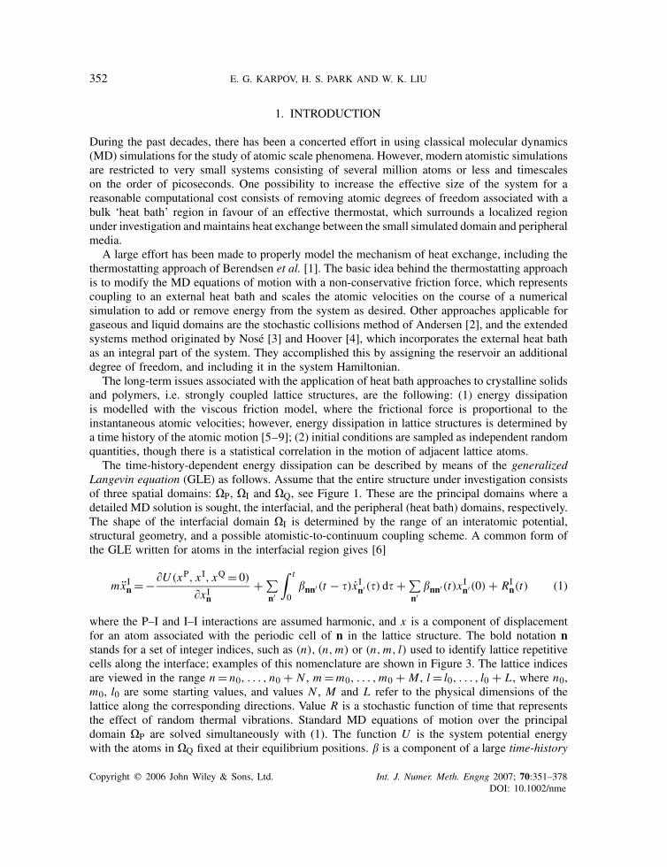
The time-history-dependent energy dissipation can be described by means of the generalizedLangevin equation (GLE) as follows. Assume that the entire structure under investigation consistsof three spatial domains: �P, �I and �Q, see Figure 1. These are the principal domains where adetailed MD solution is sought, the interfacial, and the peripheral (heat bath) domains, respectively.The shape of the interfacial domain �I is determined by the range of an interatomic potential,structural geometry, and a possible atomistic-to-continuum coupling scheme. A common form ofthe GLE written for atoms in the interfacial region gives [6]

mx In = −�U (xP, x I, xQ = 0)

�x In+∑

n′

∫ t

0�nn′(t − �)x In′(�) d� +∑

n′�nn′(t)x In′(0) + RI

n(t) (1)

where the P–I and I–I interactions are assumed harmonic, and x is a component of displacementfor an atom associated with the periodic cell of n in the lattice structure. The bold notation nstands for a set of integer indices, such as (n), (n,m) or (n,m, l) used to identify lattice repetitivecells along the interface; examples of this nomenclature are shown in Figure 3. The lattice indicesare viewed in the range n = n0, . . . , n0 + N , m =m0, . . . ,m0 + M , l = l0, . . . , l0 + L , where n0,m0, l0 are some starting values, and values N , M and L refer to the physical dimensions of thelattice along the corresponding directions. Value R is a stochastic function of time that representsthe effect of random thermal vibrations. Standard MD equations of motion over the principaldomain �P are solved simultaneously with (1). The function U is the system potential energywith the atoms in �Q fixed at their equilibrium positions. � is a component of a large time-history

Copyright q 2006 John Wiley & Sons, Ltd. Int. J. Numer. Meth. Engng 2007; 70:351–378DOI: 10.1002/nme

PHONON HEAT BATH APPROACH 353

(Heat bath)Q

P

I

Figure 1. Principal domain of interest �P in thermal contact with a peripheral region�Q. �I is an interfacial region.

kernel (THK) matrix, whose dimension is determined by the number of degrees of freedom in �I.This matrix adequately describes the response of the outer domain �Q due to disturbances in theinterfacial domain �I in terms of the I–I correlation.

One important consequence of such a formulation is that propagation of outward progressivewaves across the interface in numerical simulations takes place with virtually no artificial reflection.The waves are absorbed by the interface exactly in the same manner, as if the hypotheticaldomain �Q was actually present [6–8]. This feature of the GLE formulation is also valuable forthe purpose of multiscale atomistic/continuum simulation using the bridging scale methodology[8, 10–14]. Other approaches incorporating a finite temperature formulation in the multiscalecontext include the works by Dupuy et al. [15], E et al. [16], Qu et al. [17], Strachan and Holian[18], Curtarolo and Ceder [19], Xiao and Belytschko [20], and Park et al. [21].

For a planar interface corresponding to a specific crystallographic direction in the lattice,Equation (1) can be simplified to a form with a compact THK, which is symmetric with respectto translations along the interface. It is also convenient to rewrite the convolution integral interms of displacement values and separate the I–Q correlation as follows [7–9]:

mx In = −�U (xP, x I, xQ)

�x In(2a)

xQn =∑n′

∫ t

0�n−n′(t − �)x In′(�) d� + RQ

n (t) (2b)

Here, the convolution integral and the random term R in (2b) yield displacement components ratherthan forces, in contrast with Equation (1). The summation is accomplished along neighbouringlattice cells at the interface only. � is the compact THK, whose dimension is determined only by thenumber of degrees of freedom in one repetitive lattice cell; the subscript n−n′ indicates � is spatiallyinvariant along the interface, and depends only on the distance between the current and neighbouringcells. Displacements (2b) can be treated as dynamic boundary conditions for the standard MDequation of motion (2a). Such a treatment is convenient for the practical implementation of theGLE methodology into readily available MD codes. In case that the interface �I represents aconvex polyhedron, rather than a plane, the treatment (2) is applied separately to all faces of thepolyhedron [7, 9].



E and Huang [22] recently proposed a dynamic matching conditions for the coupled atomistic-continuum simulation of solids. The authors introduce a measure of phonon reflection at theinterface as a functional over the atomic boundary displacements sought, and find the match-ing conditions by minimizing the phonon reflection. The present method provides an alternativemethodology, which allows also inward flow of thermal energy in its current form, and is based onthe time-history integral and lattice Green’s function ideas dating back to the works by Adelmanand Doll [5, 23].

One important issue that remains open in the GLE formulation (1) or (2) is an appropriate form ofthe random thermal term R. This term represents time evolution of the atomic force or displacementwithin the harmonic model given the initial conditions only. Earlier in the literature [5, 23], and alsobelow in this paper (Section 2), an exact expression for R is shown to incorporate atomistic degreesof freedom in the entire heat bath domain; this is intractable in terms of numerical modelling.Furthermore, the random function R cannot be sampled as an independent Gaussian variable atall times, because there is a correlation of the thermal noise in lattices in both time and space (seeAppendix A.4). This correlation arises due to the coupled nature of crystal lattices, as contrastedto liquids and gases, where the thermal noise is completely uncorrelated. Finally, the term R mustrepresent the canonical ensemble.

These issues can be resolved by the approach proposed in this paper, where the random thermalnoise R possesses all the adequate statistical properties imposed by the canonical distribution,including the time/space correlations. The main idea of this approach is in the following. Forharmonic lattices, the Hamiltonian can be decoupled in the normal co-ordinates, and the set oflattice normal modes can be viewed formally as a gas of non-interactive quasiparticles, or phonons.Statistical distributions of the random amplitudes and phases of the individual normal modes canbe then derived from the Gibbs canonical distribution for the phonon gas at a given temperature T .A linear combination of the normal modes with the random amplitudes and phases provides finallythe random displacement term R.

We will focus on the displacement variant of the GLE formulation, and derive systematically anequation similar to (2), though more detailed in terms of practical implementation. Next, we derivesemi-analytical expressions for the memory kernel � and the random displacement function R fora general lattice, using the assumption that the peripheral domain �Q has a uniform temperaturefield. This implies that �Q is regarded as a heat bath or heat sink, whose temperature and internalenergy are not greatly affected by the P–Q heat exchange.

The remainder of the paper is arranged as follows: Sections 2–4 detail with the theoreticalaspects of the method. Section 5 provides applications to one- (1D) and two-dimensional (2D)lattice models, and Section 6 concludes the paper.

2. MD BOUNDARY CONDITIONS

In this section, we rewrite boundary conditions (2b) for the generalized Langevin formulation(2) in a form convenient for practical implementation in MD simulations. In the course of ourdiscussion we obtain formal semi-analytical expressions for the THK and a general form of therandom displacement term in (2b).

As mentioned in Section 1, the THK describes response of the outer domain �Q due to distur-bances originating in the principal domain �P and passing across the interfacial domain �I. Anassumption required for a straightforward characterization of the response in the outer domain is



that the interface �I can be comprised by a group of plane- or slab-like interfaces. Each of theseinterfaces is to be treated according to the formulation presented below in this paper. Such anassumption, in principle, imposes limitations on allowed shapes of the principal domain, which isexpected in the form of a convex polyhedron, though not necessarily regular. See the schematicdrawing in Figure 1. Since the principal region is only a computational domain, which does notnecessarily represent an element of intrinsic physical structure of the solid, this assumption isconsidered as acceptable. We also require that the outer domain behaves only as a thermostat orheat sink so that progressive waves entering �Q are not reflected back by peripheral boundariesof this domain.

A straight line or plane-like boundary can be defined by fixing one of the lattice site indices inthe triplet n= (n,m, l). Due to translational symmetry, we can employ any specific value of thisindex; the final results will be identical. For example, let l = 0. This problem statement correspondsto dividing the entire structure under investigation into the principal, interfacial and bulk peripheralregions in accordance with the following:

�P : l<0, �I : l = 0, �Q : l�1 (3)

We will be looking for the bulk domain response only in the immediate vicinity of the interface,i.e. only for atoms (n,m, 1). In other words, our task is to express the displacements vectorsun,m,1 in terms of un,m,0. We note that the unit (repetitive) cell, denoted by the triplet n= n,m, l,should be chosen large enough, so that atoms in the slab l = 0 interact only with atoms in the slabl = 1; this requirement is convenient for the purpose of below discussion. Such a unit cell maybe represented by the elementary Wigner–Seitz cell, or be comprised of several elementary cells,depending on the range of the lattice potential.

For atoms in the interfacial and peripheral regions, it is convenient to write the linearizedequation of motion in the form [10]:

Mun(t) −∑n′

Kn−n′ un′(t) = 0, n= (n,m, l�0) (4)

where un is a vector of displacements of atoms about their equilibrium positions in the unitcell n. K are the lattice stiffness matrices, or ‘K-matrices’, which represent linear elastic propertiesof the lattice structure. These matrices are comprised of the atomic force constants

Kn−n′ =− �2U (u)

�un�un′

∣∣∣∣∣u=0

(5)

where U is the lattice potential written in terms of the atomic displacements. Due to symmetry ofthe second-order derivative in (5), K-matrices have the following general property:

Kn =KT−n (6)

We seek a solution to the boundary value problem governed by (4), where the interfacial displace-ments un,m,0 are enforced and known, and the displacements un,m,1 are to be determined.

An important detail regarding the solution of this problem consists in realizing that the motionof the boundary atoms can be caused either by the displacements of the atoms to be kept, or byan external force acting upon the interfacial atoms in a hypothetical large lattice that extends alsofor l<0. Therefore, we assume that the motion of the boundary atoms is due to unknown external



forces, which act at l = 0. Thus,

Mun(t) −∑n′

Kn−n′ un′(t) = �l0 fn,m,0 (7)

where � is the Kronecker delta (A10).Formal application of the Laplace (A4) and discrete Fourier transforms (DFTs) (A11) to

Equation (7) gives

U(p, �) = G(p, �)F0(p, �) + R(p, �) (8)

G(p, �) = (�2M − K(p))−1 (9)

R(p, �) =MG(p, �)(�u(p, 0) + ˆu(p, 0)) (10)

where the transformed force, F0(p, �) ≡ F0(p, q, �). Substitution of this force into (8) and furtherapplication of the inverse DFT over r → l lead to

Ul(p, q, �) − Rl(p, q, �) = Gl(p, q, �)F0(p, q, �) (11)

Here, the tilde notation stands for the mixed (transform/real space) quantities that depend on land the transform variables p, q and �. The force vector F0 can be eliminated by writing twoequations (11), for l = 0 and 1, and substituting F0 from the first of these equations into the second:

U1(p, q, �) − R1(p, q, �) = H(p, q, �)(U0(p, q, �) − R0(p, q, �)) (12)

H(p, q, �) = G1(p, q, �)G−10 (p, q, �) (13)

Finally, application of the inverse DFT transform (A14) over p→ n and q →m, and the inverseLaplace transform onto (12) result in a solution of the form

un,m,1(t) = ∑n′,m′

∫ t

0d� hn−n′,m−m′(t − �)(un′,m′,0(�) − Rn′,m′,0(�)) + Rn,m,1(t) (14)

In this expression

hn,m(t) =L−1�→tF

−1p→nF

−1q→m{G1(p, q, �)G−1

0 (p, q, �)} (15a)

Gl(p, q, �) =F−1r→l{G(p, �)}, p≡ (p, q, r) (15b)

where the symbols F−1 and L−1 stand for the inverse DFT and Laplace transform, respectively.The vector R depends on the initial conditions (the capital letter R is used for both Laplace andtime domain functions)

Rn(t) =M∑n′

(gn−n′(t)un′(0) + gn−n′(t)un′(0)) (16a)

gn(t) =L−1�→tF

−1p→nF

−1q→mF

−1r→l{G(p, �)} (16b)



The time-dependent matrix function g is known as the lattice dynamics Greens function [7, 10].This function describes response of a large, non-constrained lattice to localized unit excitations,or localized perturbations of initial conditions.

Solution (14) can serve as a boundary condition to the MD equation of motion (2a), providedthat the atoms in a given plane or slab of constant l interact only with each other and with atomsin the adjacent slabs l − 1 and l + 1. For longer ranged forces, the size of the unit cell must beincreased so that this requirement is satisfied. At the same time, range of the interaction along thedirections n and m can be arbitrary. Boundary conditions of the type (15)–(16) were also discussedin [7, 9] with the assumptions that the interface is initially at rest, and temperature of the externalregion is zero at all times; within these settings, Rn(t) = 0.

Below we rewrite the boundary condition (14) in the sample extended forms corresponding to1D, 2D and 3D lattices, respectively:

u1(t) =∫ t

0h(t − �)(u0(�) − R0(�)) d� + R1(t), �I : n = 0 (17a)

un,1(t) =n+nc∑

n′=n−nc

∫ t

0d� hn−n′(t−�)(un′,0(�)−Rn′,0(�))+Rn,1(t), �I :m = 0 (17b)

un,m,1(t) =n+nc∑

n′=n−nc

m+mc∑m′=m−mc

∫ t

0d� hn−n′,m−m′(t − �)

×(un′,m′,0(�) − Rn′,m′,0(�)) + Rn,m,1(t), �I : l = 0 (17c)

For most potentials, it is proper to truncate the convolution sums at nc,mc = 4 . . . 6; such atruncation can significantly reduce computational cost of these boundary condition [7].

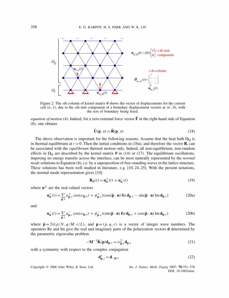
The boundary conditions in one of the forms (17) are convenient for practical implementation,because the THK (15) has a compact size of S × S, where S is the number of degrees of freedom inone unit cell only. Furthermore, matrix h is a fundamental structural characteristic of the periodiclattice; it is unique for a given lattice model and a specific crystallographic plane. This plane iscoplanar with the interface �I. The THK relates the displacement solution in �Q with the localizedboundary perturbations. The physical meaning of the kernel h is explained in Figure 2. Numericalevaluation of the time history kernel (15) is straightforward by utilizing the numerical methodsfor Laplace and DFT inversion, which are reviewed in the Appendix.

3. NORMAL MODE REPRESENTATION OF THE RANDOM NOISE

There are three important observations regarding the original structure of random displacementterm R, Equation (16), in the boundary conditions (17). First, it requires expensive evaluation ofthe lattice Green’s function g over the entire structure including the hypothetical heat bath region.Second, it requires knowledge of initial conditions for all atoms, such that the lattice is found inthermodynamic equilibrium at a given heat bath temperature T . Both of these requirements makedirect usage of the formulation impractical.

Meantime, the third observation is crucial in the sense that it allows resolving the first twoissues in a numerically tractable manner: in fact, the random vector (16) satisfies the homogeneous



... ... ... ... ...

1, (t)nu

',0(t)nu

s-th unit component

s-th column

',010

( ) (t)n tu

Q

'... ...

... ...(t)n n

1, (t)nuI

Figure 2. The sth column of kernel matrix h shows the vector of displacements for the currentcell (n, 1), due to the sth unit component of a boundary displacement vectors at (n′, 0), with

the rest of boundary being fixed.

equation of motion (4). Indeed, for a zero external force vector F in the right-hand side of Equation(8), one obtains

U(p, �) = R(p, �) (18)

The above observation is important for the following reasons. Assume that the heat bath �Q isin thermal equilibrium at t = 0. Then the initial conditions in (16a), and therefore the vector R, canbe associated with the equilibrium thermal motion only. Indeed, all non-equilibrium, non-randomeffects in �Q are described by the kernel matrix h in (14) or (17). The equilibrium oscillations,imposing no energy transfer across the interface, can be most naturally represented by the normalmode solutions to Equation (8), i.e. by a superposition of free-standing waves in the lattice structure.These solutions has been well studied in literature, e.g. [10, 24, 25]. With the present notations,the normal mode representation gives [10]

Rn(t) =u+n (t) + u−

n (t) (19)

where u± are the real-valued vectors

u+n (t) =∑

p,sa+p,s cos(�p,s t + �+

p,s)(cos(p · n)Redp,s − sin(p · n) Imdp,s) (20a)

and

u−n (t) =∑

p,sa−p,s cos(�p,s t + �−

p,s)(sin(p · n)Redp,s + cos(p · n) Imdp,s) (20b)

where p= 2�(p/N , q/M, r/L), and p= (p, q, r) is a vector of integer wave numbers. Theoperators Re and Im give the real and imaginary parts of the polarization vectors d determined bythe parametric eigenvalue problem

−M−1K(p)dp,s = �2p,sdp,s (21)

with a symmetry with respect to the complex conjugation

d∗p,s =d−p,s (22)



The index s numbers different dispersion branches, i.e. various solutions of the characteristicequation

det(�2M + K(p))= 0 (23)

There are in total S dispersion branches, where S is the number of degrees of freedom in thelattice unit cell.

The normal amplitudes and phases can be different in (20a) and (20b) for the same pair p and s,however, they should satisfy

a+−p,s = a+p,s, a−−p,s =−a−

p,s, �±−p,s = �±p,s (24)

Due to symmetries (22) and (24), any pair of terms in (20a) or (20b) corresponding to −p and pare identical. Thus, solutions (20) are comprised in total by SNc, Nc =NML, linearly independentreal-valued normal modes. Note that the value SNc is equal to the total number of vibrational andtranslational degrees of freedom in the lattice structure. Obviously, any linear combination of (20a)and (20b) will also satisfy the governing equation (4).

We note that before the disturbance from the MD domain �P reaches the interface, the interfaceis at thermal equilibrium, and we may assume that u0 =R0. Then the boundary conditions (17)yield u1 =R1, which agrees with the physical arguments behind formula (19).

Usage of the random displacement vector in the form (19) is much more effectivecomputationally, as compared to (16). Relationships (19) and (20) represent a key element ofthe proposed methodology. Further practical issues, including truncation of the sums in (20) arediscussed in Section 4.

3.1. Normal amplitudes and phases: statistical properties

Free parameters of the normal mode solution (20), the normal amplitudes and phases, can be chosenarbitrary, so that the lattice motion satisfies initial conditions, or meets specific thermodynamiccharacteristics. One such characteristic can be the equilibrium temperature T .

There are in total 2SNc free parameters: SNc normal amplitudes a and SNc phases �; S is thenumber of degrees of freedom per lattice unit cell, and Nc is the total number of unit cells. Wecan derive these amplitudes and phases in a probabilistic manner only from the knowledge of thelattice temperature T and lattice spectral properties, i.e. the normal frequencies and polarizationvectors. For this purpose we utilize the Gibbs canonical distribution

W = 1

Zexp

(− H

kBT

)(25)

which encapsulates statistical properties of a classical multiparticle system in thermodynamicequilibrium at constant temperature T and constant number of particles [10, 26–28]. Here, H isthe system Hamiltonian, Z a normalization factor, and kB the Boltzmann constant. The linearizedHamiltonian of a periodic lattice structures reads as

H = 1

2

∑nuTn Mun − 1

2

∑n,n′

uTn Kn−n′ un′ (26)



Substituting displacements (20) into this relationship and further averaging in time yields

H = Nc

2

∑p,s

a2p,s�p,s = Nc

2

∑p,s

a2p,s�2p,sp,s (27)

Here, we introduced the characteristic mass and stiffness of the normal mode

p,s =d†p,s Mdp,s, �p,s = −d†p,s K(p)dp,s (28)

which are related to the normal frequency as

�2p,s = �p,s/p,s (29)

The dagger symbol in (28) stands for a complex conjugate and transposed vector. Thus, complexlattice vibrations in the space of wave numbers can be regarded as a result of the oscillatory motionof SNc quasiparticles, characterized by the mass and stiffness � in accordance with (28). Thesequasiparticles are called the lattice phonons, and a complete set of phonons for a given latticedomain comprise a formal system known as the phonon gas.

For a harmonic lattice the phonon gas is non-interactive, as a result, the Hamiltonian (27)is additive, where the total energy is given as a sum of the energies of the individual normalnodes. For an additive Hamiltonian, the Gibbs distribution is factorized, and we can find statisticaldistributions of the normal amplitude and phase of the individual normal modes. For this purpose,we note that each pair of the random quantities (ap,s, �p,s) determines polar co-ordinates of apoint in the formal configuration space associated with the normal mode (p, s). In order to obtainstatistical distributions for a and �, we substitute expression (27) into (25) and multiply the resultby the elementary volume ap,s dap,s d�p,s

dW = 1

Z

∏p,s

ap,s exp−Nca2p,s�

2p,sp,s

2kBTdap,s d�p,s (30)

This equation represents an infinitesimal probability in the (a,�)-space. It indicates that the normalamplitudes and phases are independent random variables distributed according to

w(ap,s) = Ncap,s�2p,sp,s

kBTexp

−Nca2p,s�2p,sp,s

2kBT(31a)

w(�p,s) = 1

2�(31b)

The phases are distributed uniformly in the interval (0, 2�). As follows from (31a), the meansquare amplitude is

〈a2p,s〉 =∫ ∞

0a2p,s w(ap,s) dap,s = 2kBT

Nc�2p,sp,s

(32)

On the basis of (27) and (32), we may also obtain the mean energy of an individual mode

〈p,s〉= Nc

2〈a2p,s〉�2

p,sp,s = kBT (33)



where T is the equilibrium heat bath temperature. Remarkably, this energy is invariant for all normalmodes, and for all types of harmonic lattices. This result is in agreement with the equipartitiontheorem of statistical mechanics [26–28], proving distributions (31) to be consistent from theenergetic point of view.

4. SUMMARY OF THE METHOD

The purpose of this section is to provide a brief summary of those elements that are important interms of practical usage for the proposed method.

The most important practical result of this method are the boundary conditions (17), where therandom displacement vector is chosen in the form of a normal mode decomposition, Equations (19)and (20). These boundary conditions are applied along planar interfaces of a simulation domain,incorporating the regions �P and �I, see Figure 1 or 2. The free parameters of decomposition (20),the normal amplitudes and phases, are sampled from the statistical distributions (31) once only—atthe initial time step of the simulation. At the successive time steps, the random displacementvector R is evaluated using the normal mode decomposition (20), where a relevant value of thetime variable is utilized; meantime, the random phases and amplitudes are kept invariant at alltime steps. The distribution of normal amplitudes (31a) utilizes knowledge of the lattice spectralproperties encapsulated by the normal frequencies (23), polarization vectors (21) and characteristicmasses (28). The temperature T involved in this distribution is regarded as the heat bath, or targetsystem, temperature.

Provided that there is no input or release of energy inside �P or �I, temperature in thesedomains will be approaching the value T utilized for the amplitudes (32). At the same time,the convolution integral in the boundary conditions (17) will be damping all the non-equilibriumoscillations, represented by the difference (u0− R0), and the displacements u1 will be approachingR1 in a stochastic manner. In thermal equilibrium, statistical properties of the displacement vectoron the interface will be identical with the statistical properties of the vector R that corresponds to acanonical ensemble by the definition. In general, the mechanism of heat exchange will be identicalas in a hypothetical simulation incorporating atomistic resolution over the entire peripheral domain�Q. Furthermore, since the interfacial atoms behave as if they were a part of the large hypotheticdomain �Q in equilibrium at a given temperature, the principal domain �P will correspond to acanonical ensemble, if found in thermodynamic equilibrium with �Q.

In terms of dissipation of elastic (shock) waves and heat, the domain �Q is infinite, in principle.Propagation of long elastic waves in a peripheral domain with a specific finite geometry, can beincorporated via joint usage of this method with a hybrid MD/FEM methodology [10, 29], inparticular, with the bridging scale method [10, 12–14, 30, 31]. Within the bridging scale approach,the temperature-dependent boundary conditions of the type (17) can be applied to the fine scaledisplacement field at an interface between the atomistic and continuum regions.

Equilibrium MD initial conditions for �I and a periodic part of �P can be obtainedsimply as

un(0) =Rn(0), un(0)= Rn(0) (34)

These initial conditions automatically account for the statistical correlation between the positionsand velocities of neighbouring atoms within a strongly coupled system, such as the crystal lattice(see Appendix A.4). As a result, the random phase space vector provided by (34) is compliant



Table I. Summary of the method.

Geometry and Spectral and MD boundaryelastic properties statistical properties conditions

(23)→�p,s (15)→ hn,m(t)(5)→Kn (21)→dp,s (17)→ un,m,1(t)

(31)→ ap,s ,�p,s (19)→Rn(t)

with the Gibbs canonical distribution (25), and provides a physically adequate ‘snapshot’ of thelattice in thermodynamic equilibrium with the heat bath. In other words, conditions (34) representa typical microscopic state of a periodic lattice at temperature T .

In order to save computational effort in practical applications, the total number of modes usedfor decompositions (20) can be chosen less than SNc. For example, the low-frequency part ofthe spectrum may require truncation, when the period of vibration for the corresponding modesbecome comparable with the total time of the MD simulation. A further decrease in the numberof modes can be achieved by increasing the sampling interval for the wavenumbers in (20); forexample, the wavenumbers can be sampled from ±�/2 to ±� with a constant step �/z, where z isinteger. In all cases, the parameter Nc in (31a) and (32) must be replaced with the total number ofdistinct wavenumber triplets p= (p, q, r) employed. Since any decrease in the number of modeswill abate the initial entropy of the system, it is desirable in numerical simulations to keep a largeyet reasonable number of normal modes.

In order to achieve an accurate target temperature in the case of a limited number of modes(less than 103), one may compute the normal amplitudes for (20) simply as square roots of themean values (32), rather than sampling them from the original distribution (31a) in a probabilisticmanner. The phases of the normal modes in decomposition (20) must be randomly sampled inall instances, as values uniformly distributed over [0, 2�]. Recall that the normal amplitudes andphases are pre-evaluated once only for an entire simulation run. Then, formulas (19) and (20) areused to evaluate the vector R for any arbitrary physical time (time step) of the simulation.

We can summarize that implementation of the present formulation is comprised of threesuccessive steps, see Table I: (1) analysis of lattice geometry and evaluation of elastic propertiesin the form of K -matrices, (2) evaluation of spectral properties of the lattice, and (3) constructionof the boundary conditions. These steps are programmed in a preliminary block of a MD code, orresolved analytically when possible. Specific examples and some useful numerical strategies arediscussed in Section 5.

5. ANALYTICAL AND NUMERICAL EXAMPLES

In this section, we demonstrate practical aspects of the method in application to a 1D monoatomicchain and 2D hexagonal lattice, both with the nearest neighbour interaction. The correspondingassociate substructures are shown in Figure 3. The associate substructure fully represents themechanical properties of a periodic lattice, including the spectral and response characteristics; it iscomprised of an arbitrary (current) unit cell, (n) or (n,m) in Figure 3, and all neighbouring cellsinteracting directly with the current cell.

The chain lattice is unique in terms of the possibility to evaluate all spectral and responseproperties, along with the THK, in closed-form. The hexagonal lattice allows closed-form



( 1, 1)n m ( 1, 1)n m

( 1, 1)n m ( 1, 1)n m

( 2,n m)( 2, )n m( , )n m

x

(b)

y

( 1)n ( )n ( 1)n

(a)

Figure 3. Associate substructures of chain-like (left) and hexagonal (right) lattices withthe nearest neighbour interactions.

evaluation of only the spectral properties and the K -matrices. For more complex structures, alllattice characteristics are evaluated numerically on the basis of an interatomic potential. The spec-tral characteristics are found from (23), (21) and (28) for each specific wave vector p and branchnumber s of interest. The THK is evaluated numerically on the basis of (15).

Note that the K -matrices (5) serve as input for the THK evaluation, and they can be computednumerically as well. Numerical computation of the K -matrices is particularly reasonable forcomplex interatomic potentials, when the second-order derivatives of the lattice potential U in (5)are analytically cumbersome (even though U is written for the associate substructure only). Variousmethods for numerical computation of second-order derivatives of complex functions can be foundelsewhere in literature; special techniques accounting for the specifics of the lattice structureapplication are discussed in [32].

5.1. 1D lattice in thermal equilibrium

Consider application of the proposed heat bath approach to the monoatomic lattice chain,Figure 3(a), comprised of Na = 1001 atoms with one longitudinal degree of freedom. Obviously,the number of atoms Na and the number of unit cells Nc are identical for this lattice. The latticeis governed by the pairwise Morse potential with the Au (gold) parameters [33]

V (r) = (e2�(�−r) − 2e�(�−r)), = 0.560 eV, � = 1.637 A−1, � = 2.922 A (35)

and a cut-off radius of 1.5�. Thus, each lattice atom interacts with two nearest neighbours only,and the value � gives the equilibrium interatomic distance. In our numerical computations weutilize 1 eV, 1 ps and 1 A as the units of energy, time and length. Then, the mass unit is givenby 1 eV× 1 ps2 × 1 A−2 = 1.602× 10−23 kg. In these units, the mass of one Au atom and theBoltzmann constant are

m = 0.02042, kB = 8.6183× 10−5 (36)

Temperature is still expressed in Kelvin (K).Below, we show all successive steps for the derivation of the random vector R, and the THK h

for the boundary condition (17a). As mentioned, all these steps are possible for the chain lattice



in closed form, involving only the physical parameters from (35) and (36), and the heat bathtemperature T .

1. Equilibrium positions and co-ordinates of lattice atoms along the x-axis:

en = �n, rn(t) = en + un(t) = �n + un(t) (37)

Here, un is the displacement of the atom n; this is a one-component vector (scalar) for themonoatomic unit cell with a single degree of freedom per atom.

2. Potential energy of the lattice written for one associate cell, Figure 3(a), in terms of theatomic displacements:

U (u) ≡U (un−1,un,un+1) = V (rn − rn−1) + V (rn+1 − rn)

= V (un − un−1 + �) + V (un+1 − un + �) (38)

Here, V is the Morse potential (35).3. K-matrices (5):

K0 = − �2U (u)

�2un

∣∣∣∣∣u=0

=−4�2, K−1 =K1 =− �2U (u)

�un�un+1

∣∣∣∣∣u=0

= 2�2 (39)

where and � are the Morse parameters (35). The notation u= 0 means that we employun−1 = un =un+1 = 0 after the second-order derivatives are obtained. Notice that Kn = 0 at|n|>1. Also note that for the nearest neighbour interaction model, the value 2�2 representsthe linear stiffness constant of the interaction between two adjacent atoms

k = 2�2 = 3.0013 eV/A2 (40)

4. DFT (A11) of the K-matrices:

K(p) =∑nKne

−ipn =K−1eip + K0 + K1e

−ip = k(eip − 2 + e−ip) = 2k(cos p − 1) (41)

5. Normal frequencies (23):

(�2m+K(p))= 0→ �p = � sinp

2, � = 2

√k/m (42)

6. Polarization vectors (21):

−m−1K(p)dp =�2pdp → �2

pdp = �2pdp →dp = 1 (43)

The one-component vector dp is a constant independent of p. In general, the polarizationvectors must be normalized, therefore we utilize dp = 1.

7. Characteristic masses (28):

p =m (44)

8. Normal amplitudes (32):

ap =√

2kBT

Nc�2pm

= 1

sin p/2

√kBT

2kNc(45)



9. Random displacements, Equations (19) and (20):

Rn(t) =∑pa+p cos(�pt + �+

p ) cos pn +∑pa−p cos(�pt + �−

p ) sin pn (46)

Here, the random phases �+ and �− are sampled independently of each other. For the valuesa±p , we utilize the ensemble average amplitudes (45), rather than sampling them randomly

from the original distribution (31a).10. Transform Green’s function (9):

G(p, �) = 1

�2m + 2k(1 − cos p)(47)

11. DFT inversion (15b) for (47) at n = 0 and 1, accomplished by solving the integral (A12):

G0(�) = 1

�√m(4k + �2m)

, G1(�) = 2k + �2m − �√m(4k + �2m)

2k�√m(4k + �2m)

(48)

12. THK (15a) in Laplace domain:

H(�) = G1(�)

G0(�)=(√

�2 + 4k/m − �)2

4k/m(49)

13. THK in time domain:

h(t) = 2

tJ2(2t√k/m

)(50)

where J2 is the second-order Bessel function. Here, the Laplace transform inversion isaccomplished simply by identifying function (50) in the standard tables of Laplace transform[10, 34]. In general, inversion of the Laplace and DFTs can be accomplished numericallyby utilizing algorithms (A9) and (A14).

Having obtained the random displacement vector (46) and THK (50), we proceed to the numericalsimulation.

We sample the wave numbers p for (46) equidistantly from the interval [−�, −�/2], [�/2, �]with a step �/32. Thus, there are in total Nc = 32 distinct wave numbers, and this number isused to evaluate the normal amplitudes (45). The phases �p are sampled uniformly at (0, 2�).The corresponding normal frequencies are given by (42). A time step of �t = 0.005 was used for20 000 steps. The atoms are given initial displacements and velocities using relationships (34) fora target temperature T. For two boundary atoms at the left and right ends of the chain lattice, theboundary conditions of type (17a) are applied. This means that displacements of these atoms, u1and u1001, are enforced using a time-history of displacements of the pre-boundary atoms, u2 andu1000, respectively. Note that u2 and u1000 are computed within a standard MD solver, utilizingu1 and u1001 as dynamic boundary conditions at each time step of the simulation.

The simulation results for two target system temperatures, T= 300 and 600 K are shown inFigure 4. The MD system temperature oscillates about the target temperature exactly for theT = 300 K case. For the T = 600 K case, it oscillates about a value slightly higher than the targetsystem temperature. Nonetheless, the non-linearity results in correspondingly small errors in the



0 20 40 60 800.4

0.6

0.8

1

1.2

1.4

1.6

Normalized Time

2Ek

/ (N

a k B

T)

(a)

0 20 40 60 800.4

0.6

0.8

1

1.2

1.4

1.6

Normalized Time(b)

Figure 4. Temperature of a 1D lattice as a function of time within the phonon heat bath approach. Targetsystem temperatures T0 are: (a) 300 K; and (b) 600 K. The unit of time is

√m/k.

target system temperature, where no diverging or non-controlled behaviour is observed. For the600 K simulation, the average vibrational amplitude was 4% of the interatomic spacing, witha maximum around 20–25%; thus, the method appears accurate also in the case of moderatenon-linearities.

Another important feature of these results is that no equilibration period is required for the systemtemperature. The system temperature starts fluctuating about the correct target value immediately.Over the course of time, the decaying amplitude of fluctuations corresponds to the free energyequilibration process; though a deeper insight into this behaviour is outside the scope of thepresent paper. We only note that this effect can be explained by the gradual redistribution of thekinetic energy and potential energy between all normal modes of the system due to the non-linear correlation effects. As given by Equation (33), internal energy of a harmonic lattice inthermodynamic equilibrium is comprised by the kBT increments that are identical for all normalmodes.

The use of a larger number of normal modes in (20) should result in a faster minimization ofthe fluctuations. Indeed, Figure 5 shows the reduction in temperature fluctuations at short times inthe case of utilizing 128, instead of 32, modes. These modes are sampled for the wavenumbersin the interval [−�,−�/2], [�/2, �] with a step �/128. Thus, for a sufficiently rich normal modesampling, the system is close to a thermodynamic equilibrium with the heat bath, even at initialtimes.

5.2. Hexagonal lattice in contact with a heat source

The hexagonal lattice, as shown in Figures 2 and 3(b), is observed for the (1 1 1) crystallographicplane of a face-centred cubic (fcc) lattice. This geometry is often used in the 2D modelling of fccmetals.

Consider an orthogonal numbering of unit cells in the hexagonal lattice as displayed inFigure 3(b). Then the unit cell is represented by a single lattice atom, and the vector un showsin-plane displacements of this atom with reference to x and y Cartesian axes: un ≡un,m =



0 10 20 30 40 50 60 70 800.4

0.6

0.8

1

1.2

1.4

1.6

Normalized Time

2Ek

/ (N

a k B

T)

Figure 5. Phonon model at T0 = 600 K; the number of normal modes is increased from 32 to 128.

(uxn,m, uyn,m)T. The atomic interactions are governed by the Au Morse potential (35). Within

the nearest neighbour assumption, the associate cell is formed by a symmetric group of sevenlattice atoms as depicted in Figure 3.

Similar to the previous example, the potential energy of one associate cell in the hexagonallattice can be expressed through uxn,m , u

yn,m and �. Further use of definition (5) provides seven

non-zero K -matrices. We now provide a complete log of analytical results for the hexagonal latticegoverned by the nearest neighbour Morse potential:

1. Equilibrium positions and co-ordinates of lattice atoms:

en,m = �

2

[n

m√3

], rn,m(t) = en,m + un,m(t) (51)

2. Potential energy of one associate cell, Figure 3(b):

U = V (|rn+1,m+1 − rn,m |) + V (|rn+2,m − rn,m |) + V (|rn+1,m−1 − rn,m |)+ V (|rn−1,m−1 − rn,m |) + V (|rn−2,m − rn,m |) + V (|rn−1,m+1 − rn,m |) (52)

where V is the Morse potential (35).3. K-matrices (5), and the mass matrix:

K1,1 =K−1,−1 = k

4

[1

√3

√3 3

], K1,−1 =K−1,1 = k

4

[1 −√

3

−√3 3

]

K2,0 =K−2,0 = k

[1 0

0 0

], K0,0 = −3k

[1 0

0 1

]; M=

[m 0

0 m

] (53)



Here, the constant k is such as in (40). All other combinations of the subscript indices, suchas (1, 0), (2, 1), etc., give a zero matrix.

4. DFT (A11) of the K-matrices:

K(p, q) = k

[2 cos 2p + cos p cos q − 3 −√

3 sin p sin q

−√3 sin p sin q 3 cos p cos q − 3

](54)

5. Normal frequencies (23). There are in total two acoustic branches (s = 1, 2) for this lattice.Normal frequencies of each branch are determined by two wavenumbers, p and q:

m

k�2

p,q,s =3− cos 2p−2 cos p cos q+(−1)s√

(cos 2p− cos p cos q)2+3 sin2 p sin2 q (55)

6. Polarization vectors (21) before normalization:

dp,q,s =[3k(cos p cos q − 1) + m�2

p,q,s√3k sin p sin q

](56)

7. Characteristic masses (28):

p,q,s = dTp,q,sMdp,q,s

|dp,q,s |2 =m (57)

Obviously, this simple result is valid for any monoatomic lattice with a mass matrix of thetype M=mI, where m is the atomic mass, and I is a unity matrix.

8. Normal amplitudes. Analytical expression for the mean amplitudes is obvious from (32),(55) and (57), and we do not show it here for compactness.

9. Random displacements (19). Since the polarization vectors (56) are real valued for all p, qand s, we can write

Rn,m(t) = ∑p,q,s

a+p,q,sdp,q,s cos(�p,q,s t + �+

p,q,s) cos(pn + qm)

+ ∑p,q,s

a−p,q,sdp,q,s cos(�p,q,s t + �−

p,q,s) sin(pn + qm) (58)

10. Transformed Green’s function. An analytical expression can be made available by invertingthe 2× 2 matrix (9), where M and K are substituted from (53) and (54), in closed form.Meantime, such an expression is cumbersome.

The final steps (15) of the THK evaluation, in case of the hexagonal lattice, requirenumerical methods for the DFT and Laplace transform inversions. These methods are reviewedin the Appendix. The individual components of the resultant time-dependent function hn(t) wasdiscussed and shown for different n in an earlier publication [13].

We utilize the available random displacement vector and THK for the boundary condition (17b)in application to the 2D computational problem depicted in Figure 6. This problem statement isinspired by the great potential of nanowire applications, including the Au nanowires [35], whichwill be used as interconnects in circuits of new generation supercomputers and NEMS devices.



Nanowire

Figure 6. Left: critical region of a joint between the Au nanowire and a contact pad; right: Morsemonolayer model (the actual geometry).

Critical parts of these devices are often associated with contact, joint or cross-section points thatmay serve also a source of heat induced by higher density of electric current in the contact area.Outside the contact area, nanowire body serves mostly as a bulk absorbent of this heat. Applicationof the present methodology to this type of problems is very natural. It allows reducing size of thecomputational domain to a small region in the vicinity of the contact, where spurious heating andprobably melting of the nanowire may occur. The Au nanowire is represented by the hexagonallattice, such as in Figures 2 and 3(b). The mechanism of heat exchange with the peripheral heatsink can be modelled by GLE boundary conditions (17b) method.

The lattice structure shown in Figure 6 (right) represents the computational domain of 1836atoms to be studied. The principal domain �P spans from the first bottom to the third top horizontallayer of atoms. The interface �I is represented by the second top layer of 50 atoms correspondingto m = 0. The first top row of atoms, at m = 1, represents the hypothetical heat bath �Q at roomtemperature T = 293 K imposed by statistical properties of the random displacement term (58).Total displacements of the atoms m = 1 are governed by (17b), and they serve as dynamic boundaryconditions for the simulation over �P and �I. In the following discussion, the temperature willalways be reported as spatially averaged over the principal region �P only. Traction-free boundaryconditions are applied to the left and right edges of the structure. Atomic displacements at the bottomlayer, representing the contact area, are enforced in accordance with ux = 0 and uy = 0.22 sin 5tin order to model a friction-induced heat source.

Initial conditions are imposed in accordance with (17b) and (19) at the room temperature. Forthe normal mode sampling we utilize only the first (s = 1) branch in (55)–(56), and choose p andq from the interval [�/4, 3�/4] with a step �/40 resulting in Nc = 1600 linear-independent normalmodes. Heat generated at the bottom of the structure first lead to a rising system temperature,until a dynamic equilibrium, made possible due to the boundary condition (17b), is establishedbetween the principal domain and the heat bath. The equilibrium situation is reached at 8 fs afterthe simulation is initiated at the room temperature, Figure 7(a). The average system temperaturein �P at successive times is 663 K.

These results have been verified by a benchmark simulation by adding 160 additional atomiclayers on top of the domain shown in Figure 6 (right), and imposing the standard zero displacement



0 2 4 6 8 10 12 14 16 18100

200

300

400

500

600

700

800

900

Time, fs

Syst

em T

empe

ratu

re, K

(a)0 2 4 6 8 10 12 14 16 18

100

200

300

400

500

600

700

800

900

Time, fs

Syst

em T

empe

ratu

re, K

(b)

Figure 7. Spatially average temperature in the principal domain �P for the lattice structure shown inFigure 6: (a) present method; and (b) benchmark solution with an explicit heat bath.

boundary conditions at the peripheral top edge of the structure. The additional layers serve as aphysical thermostat for the original (smaller) system, while the benchmark model itself is notthermostatted. System temperature is still measured only in the principal region �P of the samesize as in the first simulation, and only for a period of time, within which the excitations imposed bythe heat source do not reach the peripheral boundary of the added structure. The results are shownin Figure 7(b). This benchmark simulation shows that the dynamic equilibrium is achieved in �Pafter 8 ps at a spatially average temperature of 657 K, which is close to the 663 K result obtainedwith the present method. Due to the probabilistic nature of the method, results of the computationvary slightly for different simulation runs; the results shown in Figure 7(a) and (b) represent atypical situation. As compliant with the general physics, the final (equilibrium) system temperaturedepends on the heat bath temperature chosen in this method. Lower heat bath temperatures, forinstance, including the 0K case (Rn,m = 0), would have resulted in lower system temperatures dueto smaller amplitudes of the constitutive normal components of the random displacement term (58),and thus smaller (or none at 0 K) input of energy to the system from the heat bath. Remarkably,the system temperature obtained exhibit similar trends, as in the work by E and Huang [22], whostudied a similar 2D lattice problem with frictionally generated heat at a bottom surface, absorbingboundary conditions at the top. This fact points out on a similar physical nature of E and Huang’smatching operator conditions and the present THK operator, even though these two operators adoptvarious mathematical forms.

5.3. Numerical strategies

Analytical results have been shown in Sections 5.1 and 5.2 for illustrative purposes only. In realisticapplication to complex lattice structures, a readily available quantitative form is only requiredfor the K-matrices. All successive steps in the evaluation of the lattice spectral characteristics andTHK for (19) should be accomplished numerically. A general approach to this consists of thefollowing.



Random displacements. Create a 3D array comprised of all specific values of the wavenumbersp, q and r , which will be required later for decomposition (20) of the random vector (19);assume there are Nc elements in this array. Next, compute numerically Nc matrices K(p, q, r)corresponding to all elements of the array of wavenumbers. Using these matrices, compute SNcnormal frequencies (23), polarization vectors (21), and characteristic masses (28). Then evaluateSNc amplitudes (32), and sample independently 2SNc random phases �±. Create a subroutine forcomputing the summations in (20), using the lattice site indices n, m and l and physical time t asinput parameters.

THK. Create a 4D array comprised of all specific values of the wavenumbers p, q , r and Laplaceparameter �, which will be required later for the purpose of numerical transform inversions for(15). For example, the inverse DFT procedure (A14) requires N wavenumbers p= 2� p/N , wherep=−N/2,−N/2+1, . . . , N/2−1. For each element of this array, compute numerically a matrixG(p, q, r, �), Equation (9). Next, compute the inverse r → l DFT of this matrix at l = 0 and 1, andevaluate the matrices H(p, q, �) (13) for all triplets (p, q, �). Consider these matrices as valuesof the time-history kernel in the transform domain, and use the computational algorithms from theAppendix for the DFT and Laplace transform inversions. The DFT inversions are only required at|n|�nc and |m|�mc, as follows from Equation (17c).

6. CONCLUSIONS

We have discussed a novel method to calculate the random thermal motion term R(t) in theGLE [7, 9] for the atomistic solid–solid interfaces based on a normal mode decomposition. Thefree parameters of this decomposition have been derived consistently from the lattice stiffnessparameters, with respect to temperature of the system, and characterized in a probabilistic manneron the basis of Gibbs canonical distribution. The resultant GLE, in principle, provides dynamicboundary conditions that can be utilized within a standard MD solver. These boundary conditionsprovide an accurate mechanism of heat exchange between the simulated domain and the outer heatbath, because the random term in the proposed form accounts automatically for the time/spacecorrelations of the thermal noise in the periodic lattice. As a result, the phonon heat bath capturesthe correct interfacial behaviour of the simulated structure.

Ultimately, the method allows bringing together a small and a large crystalline domain, andmodel accurately the resultant interface within the harmonic assumption for the larger (effectivelyinfinite) domain, which is excluded from the explicit numerical model. Such an interface is non-reflective for the elastic waves, as well as providing a thermostatting for the small domain, whoseinterior may incorporate arbitrary non-linearities. Example simulations with Au lattice models showthat the method preserves stability and correctness for moderate non-linearities at the interface.

We note the THK and the normal mode decomposition utilized within the phonon heat bathapproach are unique structural characteristics. Once obtained for a given lattice structure, theycan be used in solving many specific problems involving the same type of lattice. This factcomprises an advantage in terms of convenience and computational effectiveness of the presentmethod.

The present method is also interesting within the frameworks of modern numerical methodsthat couple classical particle dynamics and continuum simulations, in particular, the bridging scalemethod [11–14, 30, 31]. Note, the ‘one-scale’ equations (2) and (17) assume that the �Q region



degrees of freedom affect the �P region via the random thermal term R only. Accounting for thelarger scale �Q-to-�P elastic waves in a computationally efficient manner can be accomplishedusing the bridging scale approach. The latter separates the scales with a projector operator technique,and incorporates the random term R as a natural part of the fine scale field. Such a multiscaleapproach will allow for the two-way passage of long elastic waves across the interface, as wellas the effect of the peripheral (continuum) boundary conditions onto the atomistic region ofinterest.

One interesting possibility for the future is to utilize the fact that the present approach has acapacity to control the heat bath temperature in the course of a numerical simulation. This canbe performed by the varying normal amplitudes in accordance with relationship (32), where Tis viewed as the current (time-dependent) heat bath temperature. This feature can be particularlyuseful in a future multiscale approach allowing heat transfer over the continuum domain with adynamic temperature field.

Another topic left open for the future is a rigorous criterion for the reduced normal modesampling and resultant truncation of the wave number summations in Equation (20). This criterionshould utilize general physical arguments, such as the lattice free energy or the autocorrelationproperties of the thermal noise.

APPENDIX A

A.1. Fourier transform

The Fourier transform is used to transform a time-dependent function into the frequency space

X (�) =Ft→�{x(t)}=∫ ∞

−∞x(t) e−i�t dt (A1)

Fourier transforms obey the time-derivative theorem

Ft→�

{(��t

)n

f (t)

}= (i�)n F(�) (A2)

The inverse Fourier transform is defined as

x(t) =F−1�→t {X (�)}= 1

2�

∫ ∞

−∞X (�) ei�t d� (A3)

A.2. Laplace transform

The Laplace transform of a continuous function in time gives

X (�) =Lt→�{x(t)}=∫ ∞

0e−�t x(t) dt (A4)

where � is known as the complex frequency. The Laplace transform has the following valuableproperties: the convolution theorem

Lt→�

{∫ t

0x(t − �)y(�) d�

}= X (�)Y (�) (A5)



and the time-derivative rules

Lt→�{x(t)} = �X (�) − x(0−) (A6)

Lt→�{x(t)} = �2X (�) − �x(0−) − x(0−) (A7)

Here, the notation ‘0−’ stands for a value of the argument t ‘right before’ the zero point.Mathematically, x(0−) and x(0−) are limits of the functions x(t) and x(t), as t approacheszero from negative values.

The convolution theorem implies that the transform of a convolution integral of two functionsis equal to the product of the transforms of the individual functions. The time derivative rulesimply that the transform of a time derivative is equivalent to multiplication of a function by �.This property allows reducing differential equations to simple algebraic equations in the transformdomain, therefore, it is useful in finding analytical solutions to the classical equations of motion;see the example below in this section.

The inverse Laplace transform is defined as

x(t)=L−1�→t {X (�)}= lim

b→∞1

2�i

∫ a+ib

a−ibe�t X (�) ds, a, b∈R (A8)

However, this general mathematical definition is rarely used in practical applications. In somecases, the inverse Laplace transform for X (�), i.e. the function x(t), can be found in the standardtables, such as [34].

More generally, the inverse Laplace transform can be computed numerically. One effectivenumerical algorithm applicable to a wide range of functions was proposed by Weeks [36]. Thisalgorithm can be summarized as follows:

x(t) = ect−t/2TA∑

�=0b�L�(t/T )

b� = 2 − ��0

2T (A + 1)

A∑ =0

(Re X (� ) − cot

z 2Im X (� )

)cos(�z )

z = �(2 + 1)

2(A + 1), � = c + i

2Tcot

z 2

, T = tmax

A, c= 1

tmax

(A9)

Here, L� are Laguerre polynomials, i is the imaginary unit, X is the Laplace transform of x ; tmaxis a maximum required value of the argument for the function x , and � is the Kronecker delta,

�i j ={1, i = j

0, i = j(A10)

The value A controls the accuracy of the result, and its choice depends on tmax and the behaviourof f (t) at t ∈ [0, tmax]. For the kernel functions considered in this and following sections of thisbook, a sufficient value for A is of the order 100. Weeks’s method has been found by Daviesand Martin [37] to give excellent accuracy for the inversion of a wide range of functions. Othernumerical inversion algorithms are discussed in [37, 38].



A.3. Discrete Fourier transform

In lattice mechanics, the DFT is used to transform functional sequences, such as the displacementvector un or matrix Kn from real space to wavenumber space.

A key issue in solving the lattice equation of motion (4) or (7) is the deconvolution of theinternal force term. This is accomplished naturally with the DFT

x(p) =Fn→p{xn} =∑nxn e

−ipn, p ∈ [−�, �] (A11)

xn =F−1p→n{x(p)} = 1

2�

∫ �

−�x(p) eipn dp (A12)

which obeys the convolution theorem

Fn→p

{∑n′

xn−n′ yn′

}= x(p)y(p) (A13)

Here, the calligraphic symbol F denotes the Fourier transform operator, and the hatted notationused for the Fourier domain function.

The inverse DFT can be computed numerically by applying a trapezoidal or midpoint schemeto the integral (A12):

xn =F−1p→n{x(p)} = 1

N

N/2−1∑p=−N/2

x(2� p/N ) ei2� pn/N (A14)

Here, N is the total number of integration steps, which represents an effective size of the real spacedomain: N = nmax−nmin+1, where nmin and nmax are the minimal maximal values of the index nutilized for (A11). In application to periodic lattices, N gives the physical size of the lattice in unitcells along the corresponding translation vector. The value p in (A14) is an integer wavenumberindex, varying from −N/2 to N/2 − 1.

The nature of Fourier integrals is such that discretization procedures of the type (A14) are exact.Indeed,

1

N

N/2−1∑p=−N/2

x

(2� p

N

)ei2� pn/N = 1

N

N/2−1∑p=−N/2

(∑n′

xn′ e−i2� pn′/N)ei2� pn/N

= 1

N

∑n′

xn′N/2−1∑p=−N/2

e−i2� pn′/N ei2� pn/N

=∑n′

xn′�nn′ = xn (A15)

Provided that the function x is simple enough, the integral (A12) can be used for analyticalinversion of the DFT. Meanwhile, solutions involving a standard summation (A14) are referred toas semi-analytical.



A final valuable property of the DFT is the shift theorem,

F{xn+h} = x(p) eihp, h ∈Z (A16)

A.4. Statistical properties of the thermal noise

Vector (16a) represents a random process viewed as a combination of S random functions oftime (components of this vector). This process is characterized by a vector of mean values (firststatistical moment) and an autocorrelation matrix (second statistical moment). Since vector Requilibrium oscillations, a snapshot of this vector at t = 0 provides a set of thermodynamicallyequilibrium initial conditions, and Equation (16a) can be rewritten as

Rn(t) =M∑n′

(gn−n′(t)Rn′(0) + gn−n′(t)Rn′(0)) (A17)

The statistical moments can be conveniently written for the time derivative of the random displace-ments, i.e. for the vector R. The ergodic hypothesis of statistical mechanics assumes equivalenceof the time and ensemble averages, so that the first moment of R can be written as the ensembleaverages at some fixed time t :

〈Rn(t)〉 =M∑n′

(gn−n′(t)〈Rn′(0)〉 + gn−n′(t)〈Rn′(0)〉) (A18)

Mean values of the initial displacements and velocities are zeroes for a regular harmonic lattice,therefore,

〈Rn(t)〉= 0 (A19)

For the autocorrelation matrix function, we have

〈Rn(t)RTn′′(0)〉=M

∑n′

(gn−n′(t)〈Rn′(0)RTn′′(0)〉 + gn−n′(t)〈Rn′(0)RT

n′′(0)〉) (A20)

where we can use (e.g. [5, 23])〈Rn′(0)RT

n′′(0)〉=M−1�n′,n′′kBT, 〈Rn′(0)RTn′′(0)〉= 0 (A21)

For a monoatomic lattice, where M=mI, m is the atomic mass and I is a unity matrix, we obtain

〈Rn(t)RTn′′(0)〉= kBT

∑n′

gn−n′(t)�n′,n′′ = kBT gn−n′′(t) (A22)

More generally,

〈Rn(t + �)RTn′(�)〉= kBT gn−n′(t) (A23)

A similar result was also shown by Adelman and Doll Reference [5].Next, we can show in closed form that the normal mode decomposition (46) for the 1D

collinear lattice with the nearest neighbour interaction, Figure 3, yields the same autocorrela-tion moment (A23) obtained for the original vector (16a). Here, time derivative of the dynamicGreen’s function can be derived by multiplying (47) with �, followed by the Fourier and Laplaceinversion. This gives [10]

gn(t) = 1

mJ2n(�t), �= 2

√k/m (A24)



Employ a normal mode decomposition of R for this lattice in the form

Rn(t) =∑pap�p cos(�pt − pn + �p) (A25)

where the unity polarization vector (21) was utilized. Here, the standing waves similar to (20) areformed by pairs of the normal modes with the opposite wave numbers and equal amplitudes.

Correlation of two arbitrary normal modes from this decomposition is given by the time average

Ap,p′(t) = apap′�p�p′ limtm→∞

1

tm

∫ tm

0cos(�p(� + t) − pn + �p) cos(�p′� − p′n′ + �p′) d�

= 1

2apap′�p�p′ cos(�p� − pn + p′n′ + �p − �p′)�p,p′ (A26)

Autocorrelation of the thermal noise (A25) is then a summation over all such terms (vector Rbecomes a scalar for the present lattice model)

Rn(t + �)Rn′(�) = ∑p,p′

Ap,p′(t) = 1

2

∑pa2p�

2p cos(�p� − p(n − n′)) (A27)

Next, use the equivalence of the ensemble and time averages, which follows from the ergodichypothesis of statistical mechanics, utilize amplitudes (45) and frequencies (42), replace the sumover p by an integral, and make the change variable p= �p/N , or equivalently, p= p/2. Thisgives a result, which is in agreement with the autocorrelation property (A23) of the original randomterm

〈Rn(t + �)Rn′(�)〉 = kBT

m

1

�

∫ �

0cos(�t sin p − 2 p(n − n′)) d p

= kBT

mJ2(n−n′)(�t) = kBT gn−n′(t) (A28)

Here, we used an integral definition of the Bessel function

Jn(x)= 1

�

∫ �

0cos(x sin y − ny) dy, x, y ∈ �, n = 0, 1, . . . (A29)

ACKNOWLEDGEMENTS

The authors are grateful for the financial support from the US National Science Foundation. Manyvaluables comments by Dr Dmitry Dorofeev and Dr Albert To helped to improve the technical contentand presentation of this work.

REFERENCES

1. Berendsen HJC, Postma JPM, van Gunsteren WF, DiNola A, Haak JR. Molecular dynamics with coupling to anexternal bath. Journal of Chemical Physics 1984; 81(8):3684–3690.



2. Andersen HC. Molecular dynamics simulations at constant pressure and/or temperature. Journal of ChemicalPhysics 1980; 72(4):2384–2393.

3. Nose S. A molecular dynamics method for simulations in the canonical ensemble. Molecular Physics 1984;53:255–268.

4. Hoover WG. Canonical dynamics: equilibrium phase-space distributions. Physical Review A 1985; 31(3):1695–1697.

5. Adelman SA, Doll JD. Generalized Langevin equation approach for atom/solid-surface scattering: generalformulation for classical scattering off harmonic solids. Journal of Chemical Physics 1976; 64:2375–2388.

6. Cai W, DeKoning M, Bulatov VV, Yip S. Minimizing boundary reflections in coupled-domain simulations.Physical Review Letters 2000; 85:3213–3216.

7. Karpov EG, Wagner GJ, Liu WK. A Green’s function approach to deriving non-reflecting boundary conditionsin molecular dynamics simulations. International Journal for Numerical Methods in Engineering 2005; 62(9):1250–1262.

8. Park HS, Karpov EG, Liu WK. Non-reflecting boundary conditions for atomistic, continuum and coupledatomistic/continuum simulations. International Journal for Numerical Methods in Engineering 2005; 64:237–259.

9. Wagner GJ, Karpov EG, Liu WK. Molecular dynamics boundary conditions for regular crystal lattices. ComputerMethods in Applied Mechanics and Engineering 2004; 193:1579–1601.

10. Liu WK, Karpov EG, Park HS. Nano Mechanics and Materials: Theory, Multiscale Methods and Applications.Wiley: New York, 2006.

11. Liu WK, Karpov EG, Zhang S, Park HS. An introduction to computational nano mechanics and materials.Computer Methods in Applied Mechanics and Engineering 2004; 193:1529–1578.

12. Park HS, Karpov EG, Klein PA, Liu WK. Three-dimensional bridging scale analysis of dynamic fracture. Journalof Computational Physics 2005; 207:588–609.

13. Park HS, Karpov EG, Liu WK, Klein PA. The bridging scale for two-dimensional atomistic/continuum coupling.Philosophical Magazine 2005; 85(1):79–113.

14. Wagner GJ, Liu WK. Coupling of atomistic and continuum simulations using a bridging scale decomposition.Journal of Computational Physics 2003; 190:249–274.

15. Dupuy LM, Tadmor EB, Miller RE, Phillips R. Finite-temperature quasicontinuum: molecular dynamics withoutall the atoms. Physical Review Letters 2005; 95(6):060202.

16. E W, Engquist B, Li X, Ren W, Vanden-Eijnden E. The heterogeneous multiscale method: a review. Preprint.17. Qu S, Shastry V, Curtin WA, Miller RE. A finite temperature, dynamic, coupled atomistic/discrete dislocation

method. Modeling and Simulation in Materials Science and Engineering 2005; 13(7):1101–1118.18. Strachan A, Holian BL. Energy exchange between mesoparticles and their internal degrees of freedom. Physical

Review Letters 2005; 94(1):014301.19. Curtarolo S, Ceder G. Dynamics of an inhomogeneously coarse grained multiscale system. Physical Review

Letters 2002; 88(25):255504.20. Xiao SP, Belytschko T. A bridging domain method for coupling continua with molecular dynamics. Computer

Methods in Applied Mechanics and Engineering 2004; 193:1645–1669.21. Park HS, Karpov EG, Liu WK. A temperature equation for coupled atomistic/continuum simulations. Computer

Methods in Applied Mechanics and Engineering 2004; 193:1713–1732.22. E W, Huang Z. A dynamic atomisticcontinuum method for the simulation of crystalline materials. Journal of

Computational Physics 2002; 182(1):234–261.23. Adelman SA, Doll JD. Generalized langevin equation approach for atom/solid-surface scattering: collinear

atom/harmonic chain model. Journal of Chemical Physics 1974; 61:4242–4246.24. Ghatak AK, Kothari LS. An Introduction to Lattice Dynamics. Addison-Wesley: London, 1972.25. Born M, Huang K. Dynamic Theory of Crystal Lattices. Oxford University Press: London, 1966.26. Landau LD, Lifshitz EM. Statistical Physics. Pergamon Press: Oxford, 1980.27. Mayer JE, Mayer MG. Statistical Mechanics. Wiley: New York, 1977.28. Pathria RK. Statistical Mechanics. Butterworth-Heinemann: Oxford, England, 1996.29. Curtin WA, Miller RE. Atomistic/continuum coupling in computational materials science. Modelling and

Simulation in Materials Science and Engineering 2003; 11:R33–R68.30. Tang S, Hou TY, Liu WK. A mathematical framework of the bridging scale method. International Journal for

Numerical Methods in Engineering 2006; 65(10):1688–1713.31. Tang S, Hou TY, Liu WK. A pseudo-spectral multiscale method: Interfacial conditions and coarse gird equations.

Journal of Computational Physics 2006; 213(1):57–85.



32. Karpov EG, Yu H, Park HS, Liu WK, Wang QJ, Qian D. Multiscale boundary conditions in crystalline solids:theory and application to nanoindentation. International Journal of Solids and Structures 2006, in press.

33. Harrison DE. Application of molecular dynamics simulations to the study of ion-bombarded metal surfaces.Critical Reviews in Solid State and Materials Science 1988; 14(Suppl. 1):S1–S78.

34. Oberhettinger F, Badii L. Tables of Laplace Transforms. Springer: Berlin, 1973.35. Kovtyukhova NI, Mallouk TE. Nanowires and building blocks for self-assembling logic and memory circuits.

Chemistry—A European Journal 2002; 8(9):4355–4363.36. Weeks WT. Numerical inversion of Laplace transforms using Laguerre functions. Journal of the Association for

Computing Machinery 1966; 13(3):419–429.37. Davies B, Martin B. Numerical inversion of the Laplace transforms: a survey and comparison of methods.

Journal of Computational Physics 1979; 33:1–32.38. Duffy DG. On the numerical inversion of Laplace transforms: comparison of three new methods on characteristic

problems from applications. ACM Transactions on Mathematical Software 1993; 19(3):333–359.


Date post:	15-May-2018
Category:	Documents
Upload:	vunhu
View:	215 times
Download:	1 times

Aphononheatbathapproachfortheatomisticandmultiscale...

Documents