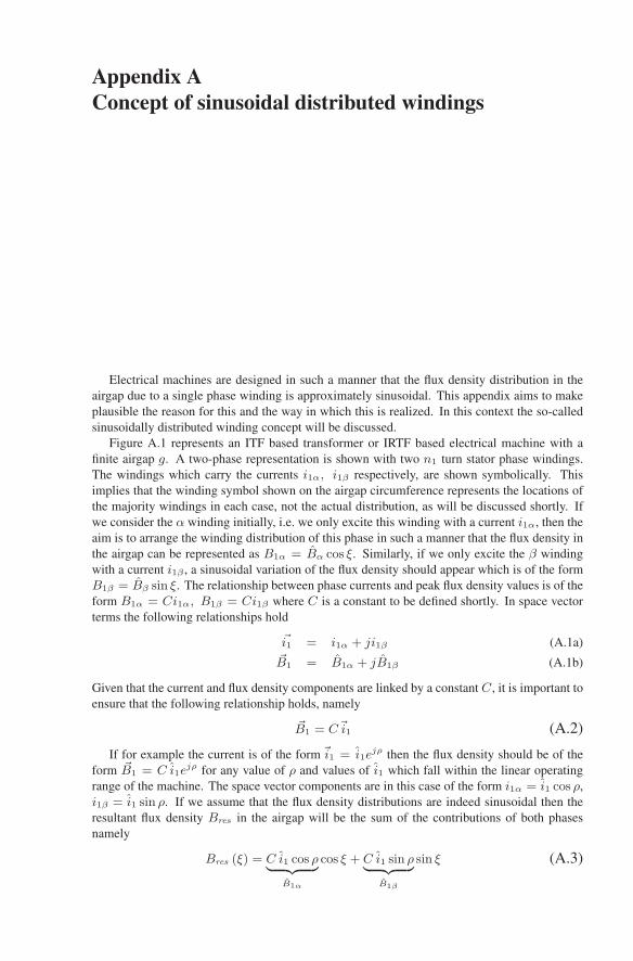
Appendix A Concept of sinusoidal distributed windings Electrical machines are designed in such a manner that the flux density distribution in the airgap due to a single phase winding is approximately sinusoidal. This appendix aims to make plausible the reason for this and the way in which this is realized. In this context the so-called sinusoidally distributed winding concept will be discussed. Figure A.1 represents an ITF based transformer or IRTF based electrical machine with a finite airgap g. A two-phase representation is shown with two n1 turn stator phase windings. The windings which carry the currents i1α, i 1β respectively, are shown symbolically. This implies that the winding symbol shown on the airgap circumference represents the locations of the majority windings in each case, not the actual distribution, as will be discussed shortly. If we consider the α winding initially, i.e. we only excite this winding with a current i1α, then the aim is to arrange the winding distribution of this phase in such a manner that the flux density in the airgap can be represented as B1α = ˆ Bα cos ξ. Similarly, if we only excite the β winding with a current i 1β , a sinusoidal variation of the flux density should appear which is of the form B 1β = ˆ B β sin ξ. The relationship between phase currents and peak flux density values is of the form B1α = Ci1α,B 1β = Ci 1β where C is a constant to be defined shortly. In space vector terms the following relationships hold i1 = i1α + ji 1β (A.1a) B1 = ˆ B1α + j ˆ B 1β (A.1b) Given that the current and flux density components are linked by a constant C, it is important to ensure that the following relationship holds, namely B1 = C i1 (A.2) If for example the current is of the form i1 = ˆ i1e jρ then the flux density should be of the form B1 = C ˆ i1e jρ for any value of ρ and values of ˆ i1 which fall within the linear operating range of the machine. The space vector components are in this case of the form i1α = ˆ i1 cos ρ, i 1β = ˆ i1 sin ρ. If we assume that the flux density distributions are indeed sinusoidal then the resultant flux density Bres in the airgap will be the sum of the contributions of both phases namely Bres (ξ)= C ˆ i1 cos ρ ˆ B 1α cos ξ + C ˆ i1 sin ρ ˆ B 1β sin ξ (A.3)
Transcript
Appendix AConcept of sinusoidal distributed windings
Electrical machines are designed in such a manner that the flux density distribution in theairgap due to a single phase winding is approximately sinusoidal. This appendix aims to makeplausible the reason for this and the way in which this is realized. In this context the so-calledsinusoidally distributed winding concept will be discussed.
Figure A.1 represents an ITF based transformer or IRTF based electrical machine with afinite airgap g. A two-phase representation is shown with two n1 turn stator phase windings.The windings which carry the currents i1α, i1β respectively, are shown symbolically. Thisimplies that the winding symbol shown on the airgap circumference represents the locations ofthe majority windings in each case, not the actual distribution, as will be discussed shortly. Ifwe consider the α winding initially, i.e. we only excite this winding with a current i1α, then theaim is to arrange the winding distribution of this phase in such a manner that the flux density inthe airgap can be represented as B1α = Bα cos ξ. Similarly, if we only excite the β windingwith a current i1β , a sinusoidal variation of the flux density should appear which is of the formB1β = Bβ sin ξ. The relationship between phase currents and peak flux density values is of theform B1α = Ci1α, B1β = Ci1β where C is a constant to be defined shortly. In space vectorterms the following relationships hold
�i1 = i1α + ji1β (A.1a)�B1 = B1α + jB1β (A.1b)
Given that the current and flux density components are linked by a constant C, it is important toensure that the following relationship holds, namely
�B1 = C�i1 (A.2)
If for example the current is of the form�i1 = i1ejρ then the flux density should be of the
form �B1 = C i1ejρ for any value of ρ and values of i1 which fall within the linear operating
range of the machine. The space vector components are in this case of the form i1α = i1 cos ρ,i1β = i1 sin ρ. If we assume that the flux density distributions are indeed sinusoidal then theresultant flux density Bres in the airgap will be the sum of the contributions of both phasesnamely
Bres (ξ) = C i1 cos ρ︸ ︷︷ ︸B1α
cos ξ + C i1 sin ρ︸ ︷︷ ︸B1β
sin ξ (A.3)
328 FUNDAMENTALS OF ELECTRICAL DRIVES
Figure A.1. Simplified ITF model, with finite airgap, no secondary winding shown
Expression (A.3) can also be written as Bres = C i1 cos (ξ − ρ) which means that the resultantairgap flux density is again a sinusoidal waveform with its peak amplitude (for this example)at ξ = ρ, which is precisely the value which should appear in the event that expression (A.2)is used directly. It is instructive to consider the case where ρ = ωst, which implies that thecurrents iα, iβ are sinusoidal waveforms with a frequency of ωs. Under these circumstances thelocation within the airgap where the resultant flux density is at its maximum is equal to ξ = ωst.A traveling wave exists in the airgap in this case, which has a rotational speed of ωsrad/s.
Having established the importance of realizing a sinusoidal flux distribution in the airgap foreach phase we will now examine how the distribution of the windings affects this goal.
For this purpose it is instructive to consider the relationship between the flux density in theairgap at locations ξ, ξ + ∆ξ with the aid of figure A.2. If we consider a loop formed by thetwo ‘contour’ sections and the flux density values at locations ξ, ξ + ∆ξ, then it is instructiveto examine the sum of the magnetic potentials along the loop and the corresponding MMFenclosed by this loop. The MMF enclosed by the loop is taken to be of the form Nξi, where Nξ
represents all or part of the α phase winding and i the phase current. The magnetic potentialsin the ‘red’ contour part of the loop are zero because the magnetic material is assumed to bemagnetically ideal (zero magnetic potential). The remaining magnetic potential contributionswhen we traverse the loop in the anti-clockwise direction must be equal to the enclosed MMFwhich leads to
g
µoB (ξ) − g
µoB (ξ + ∆ξ) = Nξi (A.4)
Expression (A.4) can also be rewritten in a more convenient form by introducing the variablen(ξ) =
Nξ
∆ξwhich represents the phase winding distribution per radian. Use of this variable
Appendix A: Concept of sinusoidal distributed windings 329
Figure A.2. Sectional view of phase winding and enlarged airgap
with equation (A.4) gives
B (ξ + ∆ξ) − B (ξ)
∆ξ= − g
µon(ξ)i (A.5)
which can be further developed by imposing the condition ∆ξ → 0 which allows equation (A.5)to be written as
dB (ξ)
dξ= − g
µon (ξ) i (A.6)
The left hand side of equation (A.6) represents the gradient of the flux density with respect toξ. An important observation of equation (A.6) is that a change in flux density in the airgap islinked to the presence of a non-zero n(ξ)i term, hence we are able to construct the flux densityin the airgap if we know (or choose) the winding distribution n(ξ) and phase current. Vice versawe can determine the required winding distribution needed to arrive at for example a sinusoidalflux density distribution.
A second condition must also be considered when constructing the flux density plot aroundthe entire airgap namely
∫ π
−π
B (ξ) dξ = 0 (A.7)
Equation (A.7) basically states that the flux density versus angle ξ distribution along the en-tire airgap of the machine cannot contain an non-zero average component. Two examples areconsidered below which demonstrate the use of equations (A.6) and (A.7). The first exampleas shown in figure A.3 shows the winding distribution n(ξ) which corresponds to a so-called‘concentrated’ winding. This means that the entire number of N turns of the phase windingare concentrated in a single slot (per winding half) with width ∆ξ, hence Nξ = N . The cor-responding flux density distribution is in this case trapezoidal and not sinusoidal as required.
The second example given by figure A.4 shows a distributed phase winding as often used inpractical three-phase machines. In this case the phase winding is split into three parts (and threeslots (per winding half), spaced λ rad apart) hence, Nξ = N
3. The total number of windings
of the phase is again equal to N . The flux density plot which corresponds with the distributed
330 FUNDAMENTALS OF ELECTRICAL DRIVES
Figure A.3. Example: concentrated winding, Nξ = N
Figure A.4. Example: distributed winding,Nξ = N3
winding is a step forward in terms of representing a sinusoidal function. The ideal case wouldaccording to equation (A.6) require a n(ξ)i representation of the form
n (ξ) i =g
µoB sin (ξ) (A.8)
in which B represents the peak value of the desired flux density function B (ξ) = B cos (ξ).Equation (A.8) shows that the winding distribution needs to be sinusoidal. The practical imple-mentation of equation (A.8) would require a large number of slots with varying number of turnsplaced in each slot. This is not realistic given the need to typically house three phase windings,hence in practice the three slot distribution shown in figure A.4 is normally used and provides aflux density versus angle distribution which is sufficiently sinusoidal.
Appendix A: Concept of sinusoidal distributed windings 331
In conclusion it is important to consider the relationship between phase flux-linkage andcircuit flux values. The phase circuit flux (for the α phase) is of the form
φmα =
∫ π2
− π2
B (ξ) dξ (A.9)
which for a concentrated winding corresponds to a flux-linkage value ψ1α = Nφmα. If adistributed winding is used then not all the circuit flux is linked with all the distributed windingcomponents in which case the flux-linkage is given as ψ1α = Neff φmα, where Neff representsthe ‘effective’ number of turns.
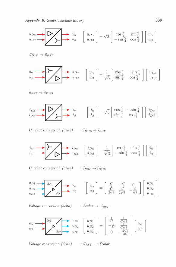
Appendix BGeneric module library
The generic modules used in this book are presented in this section. In addition to the genericrepresentation an example of a corresponding transfer function (for the module in question) isprovided. Transfer functions given, are in space vector and/or scalar format. Some modules,such as for example the ITF module, can be used in scalar or space vector format. However,some functions, such as for example the IRTF module, can only be used with space vectors.
334 FUNDAMENTALS OF ELECTRICAL DRIVES
Appendix B: Generic module library 335
336 FUNDAMENTALS OF ELECTRICAL DRIVES
Appendix B: Generic module library 337
338 FUNDAMENTALS OF ELECTRICAL DRIVES
Appendix B: Generic module library 339
340 FUNDAMENTALS OF ELECTRICAL DRIVES
References
Bodefeld, Th. and Sequenz, H. (1962). Elektrische Machinen. Springer-Verlag, 6thedition.Holmes, D.G. (1997). A generalised approach to modulation and control of hard switched con-
verters. PhD thesis, Department of Electrical and Computer engineering, Monash University,Australia.
Hughes, A. (1994). Electric Motors and Drives. Newnes.Leonhard, W. (1990). Control of Electrical Drives. Springer-Verlag, Berlin Heidelberg New York
Tokyo, 2 edition.Mathworks, The (2000). Matlab, simulink. WWW.MATHWORKS.COM.Miller, T. J. E. (1989). Brushless Permanent-Magnet and Reluctance Motor Drives. Number 21
in Monographs in Electrical and Electronic Engineering. Oxford Science Publications.Mohan, N. (2001). Advanced Electrical Drives, Analysis, Control and Modeling using Simulink.
MNPERE, Minneapolis, USA.Svensson, T. (1988). On modulation and control of electronic power converters. Technical Report
186, Chalmers University of Technology, School of Electrical and Computer engineering.van Duijsen, P.J. (2005). Simulation research, caspoc 2005. WWW.CASPOC.COM.Veltman, A. (1994). The Fish Method: interaction between AC-machines and Switching Power
Converters. PhD thesis, Department of Electrical Engineering, Delft University of Technol-ogy, the Netherlands.