Appendix D. Methods for Assessing Carbon Stocks, … D 123 Appendix D. Methods for Assessing Carbon...

Appendix D 123

Appendix D. Methods for Assessing Carbon Stocks, Carbon Sequestration, and Greenhouse-Gas Fluxes of Terrestrial Ecosystems

but it also determines uncertainty estimates of the predicted variables. GEMS previously has been applied in this way to simulate carbon dynamics for large areas in Africa (Liu, Kaire, and others, 2004) and the United States (Liu, Loveland, and Kurtz, 2004; Tan and others, 2005; Liu and others, 2006).

The spreadsheet and biogeochemical modeling approaches that will be used to quantify biological carbon sequestration and greenhouse-gas (GHG) emissions for the national assessment are described in detail in the following sections. In addition, model uncertainty, model integration with other model systems, and ecosystem-services modeling are described.

D.1. Accounting and Modeling Simulations of Carbon Sequestration and Greenhouse-Gas Fluxes

D.1.1. GEMS Accounting Using the Spreadsheet Approach

Spreadsheet approaches use a computer spreadsheet tool to simulate carbon dynamics and GHG emissions. The primary advantages of the spreadsheet approach are ease in model development and model transparency. The disadvantages of the spreadsheet approach include nonspatial or coarse spatial resolution of simulations and the relatively small number of for-mulas used in spreadsheet calculations. Nevertheless, although many processes have to be simplified or ignored, the spread-sheet approach provides reference results that are useful to com-pare with those from more process-based modeling systems.

In general, carbon accounting for almost all terrestrial sectors can be conducted using the spreadsheet approach. The 2006 Intergovernmental Panel on Climate Change (IPCC) Guidelines for National Greenhouse Gas Inventories (Intergovernmental Panel on Climate Change, 2006) pro-Intergovernmental Panel on Climate Change, 2006) pro-, 2006) pro-vides equations and factors for building GHG spreadsheets. A spreadsheet approach will be implemented in parallel to GEMS to compare and verify GEMS outputs; this method is called “GEMS-spreadsheet.”

The GEMS-spreadsheet method requires the following input data at the ecoregion level (or any geographic region):

• Land-cover transition tables during two periods (for example, 2001–2010 and 2011–2050)

• Vegetation-age distribution by land-cover type• Carbon density by age and land-cover type• GHG fluxes by vegetation age and land-cover type• The severity of disturbances or management activities

on live biomass carbon, expressed as the fraction of biomass killed or harvested

Quantifying terrestrial carbon dynamics for large regions is a challenging task for scientists (Potter and others, 1993; Intergovernmental Panel on Climate Change, 1997; Houghton and others, 1999; McGuire and others, 2002; Liu, Loveland, and Kurtz, 2004; Parton and others, 2005; Sierra and others, 2009). Generally, two approaches are used to quantify terrestrial carbon dynamics for large regions. The first of these is the spreadsheet or bookkeeping approach (Intergovernmental Panel on Climate Change, 1997; Houghton and others, 1999) that relies on a set of predefined carbon-response curves (for example, tree-growth curves) and uses regression equations or look-up tables; however, most carbon-response curves are created locally on the basis of limited categories of site conditions. They may be insufficient for capturing the effects of the spatial and temporal variability of land use, soils, and climate on carbon dynamics. The second approach depends on process-based biogeochemical models (Schimel and others, 1994; Melillo and others, 1995; McGuire and others, 2002; Chen and others, 2003; Potter and others, 2005; Tan and others, 2005; Liu and others, 2006). Instead of predefining the carbon-response curves under typical conditions, as in the bookkeeping approach, this process-based approach simulates carbon dynamics under specific and changing environmental and management conditions. Although it is capable of capturing detailed responses to changes in the driving variables, it usually requires more complicated input data and parameters.

Many site-scale process-based biogeochemical models were developed during the past 20 years (Parton and others, 1987; Running and Coughlan, 1988; Li and others, 1992). They benefited from an improved understanding of biogeochemical processes resulting from controlled experiments and field observations. For regional studies, however, these models usually were directly applied to grid cells (for example, 0.5 × 0.5 degrees longitude and latitude) that were larger than the site scale (Melillo and others, 1995; Pan and others, 1998; McGuire and others, 2001; Potter and others, 2005) without incorporating information on field-scale heterogeneities. This can result in significant biases in the estimations of important biogeochemical and biophysical processes (Avissar, 1992; Pierce and Running, 1995; Turner and others, 2000; Reiners and others, 2002). Therefore, deploying field-scale ecosystem models to generate regional carbon-sequestration estimates with measures of uncertainty is a challenge.

The General Ensemble Modeling System (GEMS) was designed to facilitate the application of classic site-scale models on a regional scale and to better integrate well-estab-lished ecosystem biogeochemical models by using a Monte Carlo-based ensemble approach to incorporate the probable occurrence of parameter values in simulations. Consequently, GEMS not only drives biogeochemical models to simulate the spatial and temporal trends of carbon and nitrogen dynamics,

124 Assessment Methodology for Carbon Stocks and Sequestration and Greenhouse Gas Fluxes—Public Review Draft

• Carbon transfer coefficients among different pools, including the atmospheric carbon dioxide (CO2) pool

• Carbon decomposition rates in various poolsThe GEMS-spreadsheet method tracks the carbon stock

of unchanged land units (that is, no land-cover transitions) in carbon pool p1 in a given region using the following account-ing procedure:

, (D1)

where n and m are the number of land-cover classes and age classes, respectively,

At,i is the total unchanged area of land-cover class i at time t,

at,i,j, and ct,i,j,p1 are, respectively, area fraction and

carbon density of land-cover class i, at time t, and in age class j.

Carbon-density values will be derived from the U.S. Forest Service’s (USFS) Forest Inventory and Analysis (FIA) program data. Land-cover transitions and age distribution information will be from the “forecasting scenarios of land-cover change” (FORE–SCE) model.

For those land units that experienced land-cover transi-tions, the following procedures are used to track carbon flow among different pools:

, (D2)

where At,i,j is the area changed from land-cover class i to j at time t;

ct,i,p1 is the average carbon density in pool p1,

and αi,j,p1→p2

is the fraction of carbon density in pool p1 that is transferred to p2 because of land-cover transition from i to j.

In the GEMS-spreadsheet method, carbon is transferred among the live and dead, aboveground and belowground bio-mass pools and the wood-products pool (harvested materials). Carbon-transfer coefficients will be developed based on expert knowledge, remotely sensed data (for example, fire severity), and output from disturbances modeling.

The decomposition of carbon in a given pool (except the live biomass pool) is calculated as follows:

, (D3)

where βp1→CO2 is the decomposition rate of carbon in pool p1,

defined as a fraction of the pool size.In summary, the carbon stocks in live biomass,

aboveground and belowground dead biomass, and wood prod-ucts in a region at time t are calculated as follows:

, (D4)

where k is the number of carbon pools.The total regional nitrous-oxide (N2O) and methane

(CH4) fluxes are calculated as follows using the GEMS-spreadsheet method:

, (D5)

where λt,i,j is the flux of N2O or CH4 per area on land-cover class i, at time t, and in age class j.

Region-specific GHG fluxes for different ecosystems under various management practices will be compiled from exten-sive literature review and metadata analysis.

D.1.2. GEMS Biogeochemical ModelingGEMS provides spatially explicit biogeochemical-model

simulations for large areas. The overall GEMS input-data

Figure D1. Diagram showing functionality and major types of input data for the General Ensemble Modeling System (GEMS). FIA, Forest Inventory and Analysis Program (U.S. Forest Service); USDA, U.S. Department of Agriculture; EDCM, Erosion-Deposition-Carbon Model; BIOME–BGC, biome biogeochemical cycles; IPCC, Intergovernmental Panel on Climate Change; FORE–SCE, “forecasting scenarios of land-cover change” model; CLUE, Conversion of Land Use and its Effects model.

Appendix D 125

requirements and model functions are shown in figure D1, which indicates that GEMS, as an expandable framework, can process various land-use and disturbance data and link with existing models and tools. GEMS uses two approaches to interact with encapsulated biogeochemical models: agent and direct implementation.

D.1.2.1. Ensemble Models or Agent ImplementationA special model interface (that is, the agent) controls

diverse plot- and regional-scale models in GEMS. This approach requires minimum or no modifications to the underlying biogeochemical models and can be useful for reusing models that are difficult to modify. Under the “agent implementation” mode, GEMS uses plot-scale ecosystem biogeochemical models to simulate carbon and nitrogen dynamics at the plot scale. It controls these site-scale mod-els by automatically parameterizing them according to the biophysical conditions of any land parcel and deploying them across space without considering the interactions among land pixels. Plot- and regional-scale biogeochemical models, such as the Century model (Parton and others, 1987), the Erosion-Deposition-Carbon Model (EDCM; Liu and others, 2003), and the Integrated Biosphere Simulator (IBIS; Foley and others, 1996), can serve as encapsulated ecosystem biogeochemi-cal models in GEMS (Tan and others, 2005; Liu and others, 2006). Because GEMS is designed to encapsulate multiple models, and parameterize and execute these models using the same data, it provides an ideal platform to conduct “model ensemble” simulations to identify and address issues and uncertainty related to model structure and mathematical repre-sentations of biophysical processes.

To ensure a nationally consistent approach for selecting biogeochemical models for the assessment, a modeling work- a modeling work-shop will be held in summer of 2010, and national ecosystem modeling experts will be invited to help identify additional

suitable models. Model selection will address the ability to consider the effects of land-use and land-cover change, major disturbances, and climate change on carbon sequestration and GHG emissions. Predefined criteria are listed in table D1; this list does not mean that a single biogeochemical model must meet all these criteria.

D.1.2.2. Direct ImplementationBiogeochemical models, such as EDCM and Century, are

merged directly with GEMS to allow more efficient, spatially explicit simulations. Many regional model applications adopt a time-space simulation paradigm, which runs a simulation for an individual pixel from beginning to end in time before moving to the next pixel. In the direct implementation (for example, GEMS–EDCM), the space-time sequence paradigm will be used instead (thus, GEMS simulates the whole region for a given time step first, then moves to next time step). The space-time sequence paradigm provides easy ways to integrate with other modeling systems such as FORE–SCE (“forecast-ing scenarios of land-cover change” model), USPED (Unit Stream Power-Based Erosion Deposition), and the disturbance models in a parallel computation fashion; lateral movements of carbon and nitrogen can be effectively quantified as well. Detailed descriptions of GEMS–EDCM, including its theoreti-cal basis, general structure, simulation capability, and unique approach are provided in the following sections.

D.1.2.3. GEMS Data Flow and Linkages With Other Modeling Products

The overall GEMS flow chart of data and processes, including the spatial simulation unit setup, the Monte Carlo process, biogeochemical-model simulation, data assimilation, network Common Data Form (NetCDF) data processing and visualization, the post-simulation process, and uncertainty

Table D1. Tentative selection criteria and checklist for biogeochemical models to be included in the General Ensemble Modeling System (GEMS).

[CO2, carbon dioxide]

Criteria Questionnaire checklist

Ecosystem processes Include ecosystem carbon, nitrogen, and water cycles?Include ecophysiological processes (for example, photosynthesis)?Consider major ecosystem disturbances (fire, logging)?Consider major ecosystem management activities?

Ecosystem types and carbon pools Include all major natural forest/shrub/grassland systems?Include agricultural ecosystems?Include wetland ecosystems?Include major vegetation and soil carbon/nitrogen pools?

Model structure and reuse Allow for parallel model simulation?Well modularized and easy to be incorporated into GEMS?Coded in familiar programming language (C/C++, Fortran)?

Scientific rigor Model is well accepted and published?The team has some experience with the model?Allow sensitivity testing on key driving variables (for example, climate, CO2)?


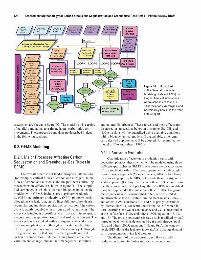
assessment are shown in figure D2. The model also is capable of parallel simulations to estimate lateral carbon-nitrogen movements. These processes and data are described in detail in the following sections.

D.2. GEMS Modeling

D.2.1. Major Processes Affecting Carbon Sequestration and Greenhouse-Gas Fluxes in GEMS

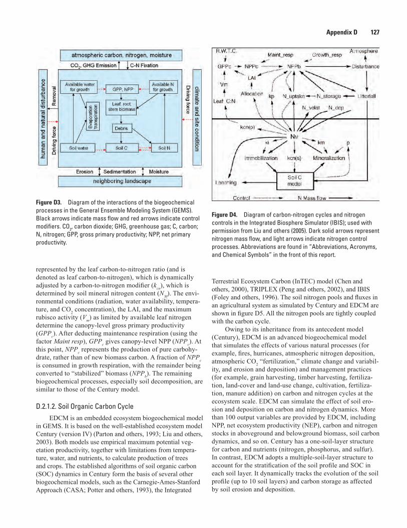
The overall processes of land-atmosphere interactions (for example, vertical fluxes of carbon and nitrogen), lateral fluxes of carbon and nutrients, and the pertinent controlling mechanisms in GEMS are shown in figure D3. The simpli-fied carbon cycle, which is the main biogeochemical cycle modeled with GEMS, includes gross primary productiv-ity (GPP), net primary productivity (NPP), photosynthesis allocations (to leaf, root, stem), litter fall, mortality, debris accumulation, and decomposition of soil carbon. The carbon cycle is tightly coupled with nitrogen and water cycles. The water cycle includes algorithms to estimate rain interception, evaporation, transpiration, runoff, and soil water content. The water cycle is also linked with soil organic carbon decom-position and plant growth through soil water availability. The nitrogen cycle is coupled with the carbon cycle through nitrogen availability that controls plant growth and soil carbon decomposition. External driving forces are climate variation and change, human land-management activities,

and natural disturbances. These forces and their effects are discussed in subsections below in this appendix. CH4 and N2O emissions will be quantified using available equations within biogeochemical models. If unavailable, other empiri-cally derived approaches will be adopted (for example, the model of Cao and others (1996)).

D.2.1.1. Ecosystem ProductionQuantification of ecosystem production starts with

vegetation photosynthesis, which will be modeled using three different approaches in GEMS to overcome the disadvantages of any single algorithm. The three approaches include a light-use-efficiency approach (Yuan and others, 2007), a biochem-ical-modeling approach (IBIS; Foley and others, 1996), and a scalar approach (Century; Parton and others, 1993). For exam-ple, the algorithm for leaf photosynthesis in IBIS is a modified Farquhar-type model (Farquhar and others, 1980). The gross photosynthesis rate through light-limited, rubisco-limited, and triosephosphate-utilization-limited mechanisms (Foley and others, 1996, equations 2, 4, and 5) is partly determined by intercellular CO2 concentration within the leaf, which in turn determines the water conductance and CO2 concentration at the leaf surface (Foley and others, 1996, equations 13, 14, and 15). The gross photosynthesis rate also is modified by leaf nitrogen level, which is determined by the soil nitrogen pool (Liu and others, 2005, equations 1, 8, and 9). At the canopy level, IBIS allows the leaf area index (LAI) to change dynami-cally depending on living leaf biomass.

The diagram of the carbon-nitrogen flow in IBIS is shown in figure D4. Foliar nitrogen concentration is

Figure D2. Flow chart of the General Ensemble Modeling System (GEMS) for biogeochemical simulations. Abbreviations are found in “Abbreviations, Acronyms, and Chemical Symbols” in the front of this report.

Appendix D 127

Terrestrial Ecosystem Carbon (InTEC) model (Chen and others, 2000), TRIPLEX (Peng and others, 2002), and IBIS (Foley and others, 1996). The soil nitrogen pools and fluxes in an agricultural system as simulated by Century and EDCM are shown in figure D5. All the nitrogen pools are tightly coupled with the carbon cycle.

Owing to its inheritance from its antecedent model (Century), EDCM is an advanced biogeochemical model that simulates the effects of various natural processes (for example, fires, hurricanes, atmospheric nitrogen deposition, atmospheric CO2 “fertilization,” climate change and variabil-ity, and erosion and deposition) and management practices (for example, grain harvesting, timber harvesting, fertiliza-tion, land-cover and land-use change, cultivation, fertiliza-tion, manure addition) on carbon and nitrogen cycles at the ecosystem scale. EDCM can simulate the effect of soil ero-sion and deposition on carbon and nitrogen dynamics. More than 100 output variables are provided by EDCM, including NPP, net ecosystem productivity (NEP), carbon and nitrogen stocks in aboveground and belowground biomass, soil carbon dynamics, and so on. Century has a one-soil-layer structure for carbon and nutrients (nitrogen, phosphorus, and sulfur). In contrast, EDCM adopts a multiple-soil-layer structure to account for the stratification of the soil profile and SOC in each soil layer. It dynamically tracks the evolution of the soil profile (up to 10 soil layers) and carbon storage as affected by soil erosion and deposition.

represented by the leaf carbon-to-nitrogen ratio (and is denoted as leaf carbon-to-nitrogen), which is dynamically adjusted by a carbon-to-nitrogen modifier (kcn), which is determined by soil mineral nitrogen content (NM). The envi-ronmental conditions (radiation, water availability, tempera-ture, and CO2 concentration), the LAI, and the maximum rubisco activity (Vm) as limited by available leaf nitrogen determine the canopy-level gross primary productivity (GPPc). After deducting maintenance respiration (using the factor Maint resp), GPPc gives canopy-level NPP (NPPc). At this point, NPPc represents the production of pure carbohy-drate, rather than of new biomass carbon. A fraction of NPPc is consumed in growth respiration, with the remainder being converted to “stabilized” biomass (NPPb). The remaining biogeochemical processes, especially soil decomposition, are similar to those of the Century model.

D.2.1.2. Soil Organic Carbon CycleEDCM is an embedded ecosystem biogeochemical model

in GEMS. It is based on the well-established ecosystem model Century (version IV) (Parton and others, 1993; Liu and others, 2003). Both models use empirical maximum potential veg-etation productivity, together with limitations from tempera-ture, water, and nutrients, to calculate production of trees and crops. The established algorithms of soil organic carbon (SOC) dynamics in Century form the basis of several other biogeochemical models, such as the Carnegie-Ames-Stanford Approach (CASA; Potter and others, 1993), the Integrated

Figure D3. Diagram of the interactions of the biogeochemical processes in the General Ensemble Modeling System (GEMS). Black arrows indicate mass flow and red arrows indicate control modifiers. CO2, carbon dioxide; GHG, greenhouse gas; C, carbon; N, nitrogen; GPP, gross primary productivity; NPP, net primary productivity.

Figure D4. Diagram of carbon-nitrogen cycles and nitrogen controls in the Integrated Biosphere Simulator (IBIS); used with permission from Liu and others (2005). Dark solid arrows represent nitrogen mass flow, and light arrows indicate nitrogen control processes. Abbreviations are found in “Abbreviations, Acronyms, and Chemical Symbols” in the front of this report.


D.2.1.3. Effects of DisturbancesNatural and anthropogenic disturbances (for example,

fires, hurricanes, tornadoes, and forest cutting) are accounted for in the land-use- and land-cover-change (LULCC) model. Ecosystem disturbances will be parameterized in the model separately because the biogeochemical consequences of these types of disturbances can be vastly different; however, the basic procedures are similar.

Historical fire perimeters and burn-severity maps are used in GEMS to indicate the timing, location, and severity level of burns. The extent and severity of a disturbance event are usually captured by remote sensing or field monitoring and also can be estimated by models, such as the First Order Fire Effects Model (FOFEM) by Reinhardt and oth-FOFEM) by Reinhardt and oth-ers (1997) and the Landscape Successional (LANDSUM) model by Keane and others (2006). The effects of burns are expressed as biomass consumption loss and mortality loss (table D2). Based on the loss rates, GEMS reallocates

biomass and soil carbon pools for each individual land pixel. Consumption loss is a direct carbon emission to atmosphere, whereas motility loss converts live biomass carbon to dead carbon pools. The disturbed ecosystem will start regrowth with a new soil nutrient pool and a new LAI calculated in the model. Calculation of other disturbance effects will follow a similar approach to that used for fire effects, but with different carbon transition coefficients among various pools. The regrowth processes following disturbances are calculated based on light and water availability, temperature, nutrient availability, and other factors. GEMS assumes tree planting will follow the clearcutting event if a plantation is prescribed in the land-cover map, otherwise natural vegetation recovery will occur.

For the national assessment, simulated future-fire-disturbance maps will be produced along with (or embedded in) the future land-use and land-cover (LULC) maps. These disturbance maps (including simulated severity levels) will

Figure D5. Diagram showing nitrogen cycling in a terrestrial ecosystem as simulated by the Century model and the Erosion-Deposition-Carbon Model (EDCM). From Metherell and others (1993), used with permission. The nitrogen cycle is tightly coupled with the carbon cycle. C/N, carbon-to-nitrogen ratio. Abbreviations are found in “Abbreviations, Acronyms, and Chemical Symbols” in the front of this report.

Appendix D 129

be linked with GEMS the same way as the LULCC maps are linked. Annual fluxes of disturbance-induced carbon loss and the legacy multiyear cumulative effects will be reported.

D.2.1.4. Effects of Management ActivitiesIn addition to natural disturbances (for example, climate

variation, geological disasters, wildfires), human management activities also play a critical role in annual ecosystem carbon fluxes and soil carbon budgets. For example, implementing conservation residue management can significantly mitigate carbon emissions from soils in comparison to conventional tillage management. The conceptual carbon-change scenarios based on explicit simulations of management effects and feed-back are shown in figure D6.

Management activities considered in the current GEMS include (but are not limited to) the following:

• Land-use changes, including conversions between land-use classes and crop rotation

• Land-management practices, consisting of — ◦ Logging event ◦ Forest fertilization ◦ Fire-fuel management, including prescribed burns ◦ Grazing (specified into various intensity classes)

Figure D6. Conceptual model of soil organic carbon (SOC) dynamics under a paired treatment of conventional tillage (CT) and no-till (NT) after initialization of cultivation from natural status. A, SOC gain upon converting from CT to NT following CT for a period of (T1–T0). B, SOC loss caused by cropping with CT since T0. Difference (D) in SOC stock between NT and CT varies with time. SOC reaches a new equilibrium at T3 under CT and T4 under NT. The rates of SOC gain and SOC loss do not coincide but are a function of the initial SOC stock level and time scale.

Table D2. Fuel-consumption effects under different burn-severity levels, based on comparison of remotely sensed burn-severity and field observations.

[This table also is used in the fire-disturbance modeling tasks to calibrate fire-emission estimates. Source: Carl Key, U.S. Geological Survey, written commun., May 28, 2009]

ComponentsConsumption (percent) Mortality (percent)

Low Moderate High Low Moderate High

Forest floor and soil

Litter/fine fuel 15–60 61–90 91–100 – – –Duff 5–30 31–70 71–100 – – –Medium fuel 10–30 31–50 51–100 – – –Heavy 5–15 16–40 41–100 – – –Soil 5–20 21–50 51–100 – – –

Understory layer

Herb 16–60 61–85 86–100 – – –Shrub-leaf-wood 10–40 41–80 81–100 – – –Shrub-leaf-wood – – – 1–20 21–70 71–100

Premature trees

Leaf 1–20 21–70 71–100 – – –Fine branch 1–20 21–70 71–100 – – –Wood – – – 1–20 21–75 76–100

Mature trees

Leaf 1–20 21–70 71–100 – – –Branch 1–20 21–70 71–100 – – –Wood – – – 1–20 21–70 71–100


◦ Tillage practices coupled with residue input ◦ Fertilization rate and manure application ◦ Irrigation

Key algorithms, such as irrigation, fertilization, and residue return, are embedded in GEMS. Data and parameter sets will be collected and compiled from existing databases and literature.

D.2.1.5. Effects of Erosion and DepositionSoil erosion and deposition affect soil profile evolution,

spatial redistribution of carbon and nutrients, and ecosystem carbon-nitrogen dynamics (Liu and others, 2003; Lal and others, 2004). Soil erosion and deposition will be simulated by using the USPED model (Mitas and Mitasova, 1998). The effects of soil erosion and deposition on soil carbon ero-sion will be quantified; the processes to be modeled include soil-profile evolution, onsite ecosystem-carbon dynamics, and offsite transport of carbon and nitrogen onto the landscape and into wetland environments and aquatic systems.

USPED is a simple two-dimensional hydrological model that is comparable to the more broadly used Univer-sal Soil Loss Equation (USLE) and Revised Universal Soil Loss Equation (RUSLE); however, unlike the USLE/RUSLE models that can predict only soil erosion, USPED also can simulate deposition on landscape and requires four major inputs only:

• Rainfall intensity, which is to be adjusted by the actual rainfall each year

• Soil erodibility factor (K factor), which is available in the U.S. General Soil Map (also called the State Soil Geographic (STATSGO2) database) and the Soil Survey Geographic (SSURGO) databases

• Field carbon factor, which is directly converted from land-cover type

• Digital elevation model (DEM) dataMost of the input requirements are the same as those of USLE/RUSLE.

USPED is suitable for GEMS because of its appropriate time step, level of complexity, capability of simulating erosion and deposition, and robustness. For linking soil carbon with erosion and deposition, EDCM adopts a multiple-soil-layer structure to account for the stratification of the soil profile and SOC in each soil layer. It dynamically keeps track of the evolution of the soil profile (up to 10 soil layers) and carbon storage as affected by soil erosion and deposition.

In EDCM, each soil-carbon pool in the top layer will lose a certain amount of carbon, if erosion happens. The carbon eroded is calculated as the product of the fraction of the top soil layer experiencing erosion, the total amount of SOC in the top 20 centimeters of the layer, and an enrichment factor for the eroded SOC to account for the uneven vertical distribution of SOC in the top layer. EDCM can dynamically update the soil layers affected by erosion and deposition.

One approach for linking USPED with GEMS is shown in figure D7. Simulated erosion and deposition are grouped into discrete classes, which will be included in the GEMS spatial simulation unit (joint frequency distribution (JFD) cases; see later explanations), to represent the land and water surfaces of the study area. Losses of carbon and nitrogen dur-ing lateral sediment transportation are accounted for using an oxidation factor.

D.2.1.6. Fate of Wood ProductsCarbon in wood products, landfills, and other offsite

storage can be significant in the accounting of terrestrial carbon-sequestration capacity (Skog and Nicholson, 1998). Currently (2010), GEMS does not track the fate of carbon in wood products. Because GEMS is linked directly to the data-management system for the purposes of reporting and dissemination of assessment results, a spreadsheet summa-rizing sequestration and GHG fluxes across ecosystems and carbon pools will be created. Most of the carbon pools will be simulated at a pixel level. For wood products, average values will be provided. The U.S. Environmental Protection Agency (EPA) and the USFS will be consulted about the proper way to estimate forest-product carbon and potential collaboration opportunities. Existing factors and equations about harvested-wood-product carbon pools (Smith and others, 2006; Skog, 2008) will be adopted and modified to link with GEMS to track the fate of harvested wood.

D.2.1.7. Methane and Nitrous-Oxide Fluxes

The emission of CH4 at wetland sites will be simulated in terms of soil biogeochemical processes, including CH4 production by methanogenic bacteria under anaerobic condi-tions, oxidation by methanotrophic bacteria under aerobic

Figure D7. Diagram linking the erosion-deposition model (USPED; Unit Stream Power-Based Erosion Deposition) with the terrestrial biogeochemical model (EDCM; Erosion-Deposition-Carbon Model) in GEMS (General Ensemble Modeling System). A JFD (joint frequency distribution) case indicates one or more pixels with the same site condition. DEM, digital elevation model.

Appendix D 131

conditions, and transport to the atmosphere (Conrad, 1989). The principal controls of these processes are soil moisture, water table position, soil temperature, availability and quality of suitable substrates, and pathways of CH4 transport to the atmosphere. A wide range of models have been developed to simulate the plot-scale processes of CH4 generation, con-sumption, and transport (Li and others, 1992; Cao and others, 1996; Potter, 1997; Walter and others, 2001; Zhuang and others, 2006). A simple compartmental (zero-dimensional) model was developed by Cao and others (1996) to simulate wetland carbon dynamics for large areas. Another model by Potter (1997) simulated CH4 production rates from a microbial production ratio of CO2 and CH4, which changed as a function of the water-table depth. Slightly more com-plex one-dimensional models (Walter and others, 2001; Zhuang and others, 2006) also are available to tailor more detailed process descriptions. Some of these models have a detailed representation of plot-scale vertical soil processes. The deployment of these models for large areas, however, has been challenging because of the difficulties in defining parameters for these models and in simulating some of the critical driving variables, such as water-table position in individual wetlands for large areas.

The GEMS modeling team has applied the denitrifi-cation-decomposition (DNDC) model to simulate CH4 and N2O fluxes in the Prairie Pothole Region. A process-based model for CH4 that is similar to the Cao and others (1996) and DNDC approaches has been implemented in GEMS that will balance the needs of considering the plot-scale processes and the feasibility of deploying the plot-scale model for large areas to address spatial heterogeneity. Estimates of CH4 production by the model depend on the substrate availability (soil carbon and vegetation root carbon) and soil condition (soil tempera-ture, redox), whereas CH4 oxidation is calculated based on the soil redox condition or water table.

In a zero-dimensional modeling approach, the CH4 emission from wetlands to the atmosphere is calculated as the difference between the CH4 production and oxidation:

, (D6)

where MERt is the emission mass of CH4 per unit surface area of a wetland at time t,

MPRt is the production mass of CH4 per unit surface area of a wetland at time t, and

MORt is the oxidation mass of CH4 per unit surface area of a wetland at time t.

MPRt and MORt are estimated on the basis of such controlling factors as decomposed organic carbon, water-table position, soil temperature, and primary production of existing plants. These controlling factors are parameterized by applying or synthesizing techniques described in Cao and others (1996), Potter (1997), Walter and others (2001), and Zhuang and oth-ers (2006). A reasonably accurate prediction of the water-table position, in particular, is a challenging aspect. Further details are given below in section D.3.2 as part of a discussion on modeling lateral fluxes in and out of wetland systems.

Various models exist for simulating N2O emissions (for example, Li and others, 1992; Liu and others, 1999; Parton and others, 2001; Hénault and others, 2005). Procedures for estimating N2O emissions from ecosystems were developed in the prototype of the GEMS–EDCM method and applied to simulate and project N2O emissions in the Atlantic zone of Costa Rica (Liu and others, 1999; Reiners and others, 2002). Nitrification and denitrification processes are the primary processes that lead to the emission of N2O from soils. Atmo-spheric and terrestrial (for example, fertilizer, litter) deposi-tions of nitrogen, plant uptake, mineralization, and leaching can act as the major controls. The existing GEMS algorithms for N2O flux simulations will be used to compare simulation results with observations (for example, GRACEnet) and to improve the model when necessary. A zero-dimensional model is also applicable for estimating N2O emissions from wetlands:

, (D7)

where NOEt is the N2O emission mass per unit surface area of a wetland at time t,

NOEdenit,t is the production mass by denitrification per unit surface area of a wetland at time t, and

NOEnit,t is the production mass by nitrification per unit surface area of a wetland at time t.

NOEdenit,t and NOEnit,t are quantified by applying or synthesiz-ing techniques described in Li and others (1992), Liu and others (1999), Parton and others (2001), and Hénault and others (2005).

Subject to the availability of observation data, empiri-cal regression models also can be developed for emissions of CO2, CH4, and N2O from wetlands with different land-cover types, as well as hydrologic and meteorological regimes. Much of the variations of CO2 and CH4 may be explained by considering wetland soil temperature and water-table eleva-tion as predictor variables. Variations of N2O flux also could be captured by regressing with soil temperature and water-filled pore space as the predictor variables; however, such regression models likely are highly site-specific and require large datasets given their purely statistical nature. Because such datasets rarely exist in current literature, deployment of such models in large spatial, as well as temporal, scales can hardly be justified as reliable given the uncertainty of estimated regression coefficients.

The IPCC tier 1 approach (Intergovernmental Panel on Climate Change, 2006) is a simple way of obtaining crude estimations of CO2, CH4, and N2O emissions from wet-lands. The approach is based on some aggregate measures of emissions of specific GHG per unit of time and wetland area. Although IPCC (2006) provided global estimates of these emission factors based on existing literature, regional estimates for the wetlands in the United States also may be obtained from a comprehensive literature survey. Emission estimates obtained through the tier 1 approach would comple-ment the evaluations of results of the simple biogeochemical models described previously.


D.2.2. GEMS Spatial Simulation UnitThe spatial heterogeneities of the biophysical vari-

ables (such as land cover, soil texture, and DEM) often are represented on thematic maps and stored in georeferenced geographic information system (GIS) databases. The simula-tion unit in GEMS is a cluster of land pixels sharing a unique combination of values of environmental driving variables. Combining multiple input raster layers (maps) on a cell-by-cell basis in a GIS, a JFD table can be created to list all unique combinations of the values of the overlay variables and their associated frequencies (areas or number of pixels). Each unique combination forms a GEMS simulation unit. The geographic locations of all the JFD cases are uniquely determined by the JFD map, thereby providing the spatial framework to visualize and analyze the spatial and temporal patterns of biogeochemical properties and processes.

Two examples of the JFD map are shown in figure D8. The first example (fig. D8A) overlays the soil and land-cover maps; the resulting JFD map shows the unique combinations of soil and land-cover conditions. An important feature of this JFD approach is the elimination of the need to perform model simulations pixel by pixel. One pixel represents all the pixels of a JFD case. The second example (fig. D8B) shows the land pixel sampling at certain spatial intervals (for example, 5 kilometers) on a stack of relatively higher resolution (for example, 30- to 250-m) maps. This sampling approach is used when there are too many land pixels and map layers. It also creates a JFD table where each JFD case contains one land pixel only.

D.2.3. Using Ensemble Simulations to Reconcile Nonlinearity and Heterogeneity

Studies indicate that averaging across the spatial and temporal heterogeneity of the input data could have significant effects on the carbon simulations (Avissar, 1992; Pierce and Running, 1995; Turner and others, 1996; Kimball and others, 1999). This indicates that incorporating ecosystem heterogene-ity is necessary to accurately upscale carbon dynamics from site to regional scales. The direct approach of incorporating variance and covariance of input variables in the simulation process can be expressed as the following:

, (D8)

where E is the operator of expectation, p is the nonlinear model, X is a vector of model variables, n is the number of strata or total JFD, and F is the frequency of cells or the total area of strata

i as defined by the vector of Xi.Any difference between the model scale and the spa-

tial resolution of the data may introduce biases caused by model nonlinearity. An ensemble approach can assimilate the fine-scale heterogeneities in the databases to reduce potential biases. The mean value of a variable (for example, carbon stock and flux) of simulation unit i in equation D8 can be esti-mated by using multiple stochastic model simulations:

, (D9)

where m is the number of stochastic fine-scale model runs for simulation unit i, and

Figure D8. Diagram showing approaches to produce a joint-frequency distribution (JFD) map. A, Overlaying multiple map layers to create unique JFD cases from all land pixels. B, Spatial sampling at certain intervals.

Appendix D 133

Xij is the vector of model input values at the fine scale generated using a Monte Carlo approach within the space defined by Xi.

As a result, input values for each stochastic model run are sampled from their corresponding potential value domains (Xi) that usually are described by their statistical information, such as moments and distribution types. The variance of the model simulations on regional scale can be quantified as follows:

, (D10)

where the variance and covariance of the model simulations on unit i can be expressed as follows:

and (D11)

. (D12)

Other descriptive statistics, such as skewness, also can be calculated from the ensemble simulations. These moments characterize not only the spatial and temporal trends and patterns of simulated variables, but also their uncertainties in space and time.

Solving equation D10 will require excessive computational effort if the number of strata n is quite large; however, if p(Xi) and p(Xj) are independent among a great number of strata, computations will be dramatically reduced because covariance defined in equation D12 will be zero. Hence, actual applications should sufficiently identify the independence among strata. For example, suppose p(Xi) and p(Xj) represent soil organic carbon within strata i and strata j, respectively, and their random properties result from the randomness of soil texture and precipitation. If there is no lateral flow between strata i and strata j, then p(Xi) and p(Xj) can be regarded as independent.

D.2.4. Automated Model Parameterization (Monte Carlo Downscaling)Models developed for site-scale applications need linkages with georeferenced data to be

deployed across a region. Most information in spatial databases is aggregated to the map-unit level as the mean or median values, making the direct injection of georeferenced data into the modeling processes problematic and potentially biased (Pierce and Running, 1995; Kimball and others, 1999; Reiners and others, 2002). Consequently, an automated model parameterization process usually is needed to incorporate field-scale spatial heterogeneities of state and driving variables into simulations. A Monte Carlo approach is built into GEMS to downscale aggregated information from map-unit level to field scale. Examples of data variables to be downscaled for parameterization include soil property, tree age, crop rotation, and forest cutting. The following describes the automated stochastic soil and forest-age initializations.

Soil polygons on the STATSGO2 and SSURGO maps are represented by map units; each has a unique map-unit identifier (ID), size, and location. Each map unit contains from 1 to 20 soil components, representing distinct soils types. Each soil component has a soil attributes table; however, the locations of the soil components within a map unit are not known. In GEMS, for any specific stochastic simulation, a soil component was randomly picked from all components within a soil map unit according to the probability defined by the areal fractions of the components. Once the component was determined, soil characteristics were retrieved from the corresponding soil component and layer attribute databases. For the variables with increased (Vhigh) and decreased (Vlow) values, the following equation was used to assign a value (V) to minimize potential biases from model nonlinearity (Pierce and Running, 1995; Reiners and others, 2002):

(D13)

where p is a random value that follows standard normal distribution N(0,1).The above equation assumes that the possible values of the soil characteristics follow a normal distribution with 95 percent of the values varying between Vhigh and Vlow.


The Monte Carlo approach also is used to downscale regional initial forest age. The currently available forest-age data come from State- or county-level forest-inventory statis-tics. The forest-age class distribution (area weight) is a feature on the regional scale. To assign a forest age for a specific location, a cumulative probability curve must be created on the basis of the forest-age class distribution (fig. D9). The next step is to generate a random p value between 0 and 1. The p value will point to a specific level on the cumulative prob-ability curve and match it to a corresponding age class. GEMS then uses a look-up table to retrieve initial forest biomass based on the age (Liu, Liu, and others, 2008).

D.2.5. Data AssimilationData assimilation techniques can be activated to constrain

GEMS simulations with various observations at different spatial and temporal scales. Different data-assimilation techniques are implemented in GEMS to leverage the advantages and disadvan-tages of each method. For example, the Markov Chain Monte Carlo (MCMC) method is computation intensive and, therefore, difficult to apply to a region where the number of simulation units is large. It can be effective and ideal, however, to derive repre-sentative values and their uncertainties of model parameters from limited point observations, such as flux-tower measurements.

Other data assimilation techniques used by GEMS include model inversion using PEST (EPA’s model-indepen-dent parameter estimation application; http://www.epa.gov/ceampubl/tools/pest/) (Liu, Anderson, and others, 2008), Ensemble Kalman Filter (EnKF) (Evensen, 1994, 2003), and Smoothed Ensemble Kalman Filter (SEnKF) (Chen and others, 2006, 2008). Model inversion with the PEST package is based on optimal theory and thus requires that the model have a smooth response to model parameters. Both EnKF and SEnKF are based on statistical Bayesian theory and joint technology of Monte Carlo sampling with a Kalman filter.

EnKF has many successful applications in weather forecast-ing and hydrology through incorporating various data into the model simulation process to improve estimation of model state variables. The GEMS team has used some of the approaches to derive model parameter information from plot measure-ments of carbon and nitrogen stocks (Liu, Anderson, and oth-ers, 2008) and from eddy-covariance flux-tower observations (Chen and others, 2008). A combination of data-assimilation techniques will be used to ensure that model simulations agree well with observations from different sources and scales.

Plot-scale.—FLUXNET (the flux network) and FIA data (plot-scale repetitive measurements of biomass stocks and veg-etation dynamics) will be used to derive information on model-parameter values and their uncertainty. The derived model-parameter information at the plot scale will then be extrapolated to regional and national scales (Liu and others, 2008).

Regional to national scales.—EnKF, SEnKF, or other data-assimilation techniques will be used to assimilate remotely sensed and ground-based observations. For example, Zhao and others (2010) successfully assimilated the gross primary productivity (GPP) data of the Moderate Resolution Imaging Spectroradiometer (MODIS) products to support regional model simulations of carbon sequestration in a southeastern region

The SEnKF (Chen and others, 2006, 2008) will be used at the plot and regional scales. By combining EnKF with a kernel smoothing technique, SEnKF has the following characteristics:

• Simultaneously estimates the model states and param-eters through concatenating unknown parameters and state variables into a joint state vector

• Mitigates dramatic, sudden changes of parameter val-ues in the parameter-sampling and parameter-evolution process, and controls the narrowing of the parameter variance

• Recursively assimilates data into the model, and thus detects the possible time variations of parameters

• Properly addresses various sources of uncertainty stem-ming from input, output, and parameter uncertainties

In GEMS, the SEnKF procedure becomes regular Monte Carlo analysis at the time steps when no observation data are avail-able for assimilation.

The SEnKF method was tested by assimilating observed fluxes of CO2 and environmental driving-factor data from an AmeriFlux forest station (located near Howland, Me.) into a model for partitioning eddy-covariance fluxes (Chen and oth-ers, 2008). Analysis demonstrated that model parameters, such as light-use efficiency, respiration coefficients, and the mini-mum and optimum temperatures for photosynthetic activity, are greatly constrained by eddy-covariance flux data at daily to seasonal time scales.

The SEnKF stabilizes parameter values quickly regard-less of the initial values of the parameters. Predictions made by SEnKF with data assimilation matched observa-tions substantially better than predictions made without data

Figure D9. Monte Carlo downscaling of State- and county-level forest-age data to pixel level. From Liu, Liu, and others (2008), used with permission.

Appendix D 135

ecosystem carbon-nitrogen dynamics. LULCC maps generated by the model will be used to produce spatial simulation units either by the JFD approach or a land pixel sampling approach. For an individual plot, an LULCC file, called the “event schedule file,” will be created. This file specifies the type and timing of any LULCC events, as well as the type and timing of management practices, such as cultivation and fertilization.

The LULCC information from the land-change model and other information (for example, the USDA Natural Resources Inventory (NRI) database) will be assimilated using the following procedures:

• Events such as forest clearcutting, deforestation, urban-ization, and reforestation will be directly incorporated. A biomass removal or restoration algorithm will be applied to land pixels with these land-use-change events.

• Although annual clearcutting events will be provided by the land-change model, selective cutting events (for example, group-selection harvesting and fuel treatment) are not available. The selective cutting activities can be scheduled based on selective cutting rates derived from other sources, such as FIA databases, the new vegetation change tracker (VCT) product derived from LANDFIRE (Huang and others, 2009), and forest fuel-treatment data. GEMS can aggregate the total selective cutting area to an equivalent amount of clearcutting area and randomly assign the derived clearcutting to the forest landscape.

assimilation (fig. D10). Additionally, this approach also is efficient in finding the optimum parameters (fig. D11).

D.2.6. Input and Output Processor and NetCDF Interface

A GIS program (JFD Builder) was developed for generating a JFD table from primary input data layers. A NetCDF program (called NCWin) for processing and visualizing NetCDF data also was developed. All mapped data (for example, climate, soil, vegetation cover, disturbance events) are saved in NetCDF format in GEMS. The NCWin graphical user interface (GUI) provides the capability to con-vert and visualize input and output maps as well as temporal data trends (fig. D12).

D.3. Integrating With Other Models

D.3.1. Linkages With Land-Use- and Land-Cover-Change Data and Projections

For the national assessment, GEMS will be directly coupled with the land-use-change model FORE–SCE (appendix B of this report) to account for the effects of past land-cover and land-use changes and simulated future land-use changes on

Figure D10. Graphs showing an example of Smoothed Ensemble Kalman Filter (SEnKF) data assimilation on state variables. The “GEMS” curve represents the GEMS model without data assimilation. The “Data Assimilation” curve represents the GEMS model with data assimilation. Field observations (red squares) are from the online data archive of American Flux Network (AmeriFlux) sites.

Figure D11. Graphs showing the results of parameter estimation for the plant-production submodel using the Smoothed Ensemble Kalman Filter (SEnKF) in the biogeochemical General Ensemble Modeling System (GEMS). The graphs show seasonal variations of the potential plant-production rate in croplands (left) and in forests (right). The seasonal variations imply that the structure of the plant-production model might not be adequate to represent the seasonality of crop growth.


GEMS also will calculate specific thinning effects on biomass and soil carbon change when related publica-tions and field data are synthesized.

• Mapping crop species distribution and rotations for large areas is still a primary challenge for national land-cover database development. Crops are aggregated into broad categories (for example, row crops, and other agricul-tural land). It is necessary to downscale aggregated classes into specific crops for biogeochemical modeling because different crops have different biological char-acteristics and management practices, likely resulting in different effects on carbon dynamics in vegetation and soils. Disaggregation of the agricultural land data is done stochastically in GEMS based on crop composi-tion statistics at a district or county level. For example, in the U.S. Carbon Trends Project (Liu, Loveland, and Kurtz, 2004; Tan and others, 2005; Liu and oth-ers, 2006), schedules of cropping practices, including shares of various crops and rotation probabilities, were derived from the NRI database developed by the USDA Natural Resources Conservation Service. The NRI database is a statistically based sample of land-use and natural-resource conditions and trends on non-Federal lands in the United States. The inventory, covering about 800,000 sample points across the country, is done once every 5 years. Management practices, such as cultiva-tion and fertilization, are incorporated into the LULCC sequences generated for the site according to crop or forest types and geographic region.

D.3.2. Linkages With Aquatic and Wetland Systems

The carbon and nitrogen fluxes within the aquatic ecosys-tems of wetlands, lakes, rivers, and streams, as well as their lateral interactions with the terrestrial ecosystems and verti-cal exchanges with the atmosphere, will be quantified within the integrated framework of GEMS through an encapsulated

aquatic biogeochemical model. A general framework for the aquatic model, which is primarily developed at the site scale, is presented in figure D13.

The primary methodology related to aquatic and wetland systems is described in section D.2.1.7 and appendix E of this report. This subsection focuses on the geospatial aspects and heterogeneity of wetland conditions and processes for large areas. Wetlands are important systems that likely play a pivotal role in the sequestration or release of GHG gases. Physical processes such as the hydrology of flooding (which often is intermittent) and associated soil saturation can be considered as some of the common, principal drivers of wetland biogeochemistry. A functional wetland ecosystem can be conceptualized by interactions among the four major components of water, nutrients, habitat (plants and soils), and animals. A schematic diagram of these functional components and interactions is shown in figure D14.

Given the wide variety of coastal and inland wetlands and the wide range of biophysical and climate conditions across the country, it is very difficult to simulate the hydrologi-cal dynamics (for example, water table position) for indi-vidual wetlands for large areas using a purely process-based approach. The major challenges for testing and implement-ing these models include the limited availability of reliable datasets and proper parameterizations of important driving forces and boundary conditions. To address this challenge, a hybrid modeling approach, combining the process modeling and empirical modeling, is being developed to simulate water storage and water-table dynamics in wetlands. Model simula-tions will be used to derive relatively robust representations of water storage and water-table dynamics for different types of wetlands, such as permanent to semi-permanent and ephem-eral to transitional. A frame-based state-transition approach will then be used along with prior knowledge to describe hydrological regimes for different wetlands under various meteorological conditions across the country.

The wetland approach (described in section D.2.1.7 of this report, as well as the river-stream-lake-impoundment

Figure D12. Screen capture showing an example of the NCWin map and data trends graphical user interface.

Appendix D 137

methodology in appendix E of this report, will ingest the upland-erosion and organic-carbon data from GEMS as inputs of lateral fluxes from the terrestrial systems. Statistical analyses and findings of the aquatic team can contribute to the calibration, validation, and improvements of the wetland models for realisti-cally simulating the greenhouse-gas fluxes to the atmosphere and evaluating the carbon sequestration of wetland ecosystems.

D.3.3. Feedback Among the ModelsModel integration is a critical step in the project because

there are time- and space-dependent feedbacks among the different modeling components. For example, FORE–SCE requires information about the site fertility or the SOC level from GEMS to optimize the allocations of crops in space and time. On the other hand, land-disturbance information will affect the land-use behaviors, such as timber harvesting. With-out stepwise coupling between FORE–SCE and the distur-bances model, timber harvesting activities might still be pre-scribed in areas where biomass has been completely consumed by fire in the disturbances model. Carbon or biomass stock (fuel load) will strongly affect the probability of fire occur-rence and the severity of fires, which requires the coupling between the disturbances model and GEMS, with the latter providing carbon-stock information. Model integration will be accomplished on a parallel-processing computer system.

D.4. Relations With Evaluation of Ecosystem Services

Mitigation opportunities that are considered as manage-ment scenarios are evaluated with a spreadsheet approach. These opportunities will be modeled using GEMS. Examples of GEMS data products supporting mitigation opportunities (including ecosystem-services evaluation) are carbon stocks, CH4, N2O fluxes, soil erosion, NPP, wood harvests, surface

Figure D13. Diagram showing a simplified conceptualization of carbon (C) and nitrogen (N) fluxes, as well as their controls and driving forces, for an encapsulated aquatic biogeochemical model in GEMS. Solid arrows indicate mass flow and dashed arrows indicate controls or driving forces. Abbreviations are found in “Abbreviations, Acronyms, and Chemical Symbols” in the front of this report.

Figure D14. Diagram of conceptual wetland ecosystems and interactions among the functional groups. (Modified from Fitz and Hughes (2008), used with permission.)


runoff, and crop yields. In addition, linkages to ecosystem-service evaluation methods (section 3.3.6) will be built based on GEMS output.

The Energy Independence and Security Act of 2007 (EISA) (U.S. Congress, 2007) requires that “short- and long-term mitigation or adaptation strategies” be developed as an outcome of the assessment. In chapter 1 of this report, this was interpreted as a requirement to develop relevant data products and information packages that can be used conveniently by land managers and other stakeholders to develop specific strategies; however, what is “good” from the perspective of one user may be “bad” to another. Land-use change and climate change affect a myriad of ecosystem services simultaneously; some identified specific ecosystem services may be misleading because the overall effect on the ecosystem is not evaluated. Hence, a broader perspective and context is needed to evaluate and understand concur-rent effects on multiple ecosystem services. To solve this problem, a platform will be established to project changes in ecosystem services to support adaptive land-management practices. This provides a spatially explicit platform that can accommodate a diversity of land uses and climate change for simultaneous evaluations to better understand biophysical response and tradeoff analyses, highlighting relative effec-tiveness and efficiency of management activities.

A distributed geospatial model-sharing platform (fig. D15) will be used to model ecosystem services and pro-vide decision support. This platform is necessary to facilitate sharing and integrating geospatial disciplinary models. A platform based on Java Platform Enterprise Edition (J2EE) and open-source geospatial libraries (Feng and others, 2009) is in development. Shared models on the platform are accessible to applications through the Internet using the Open Geospatial

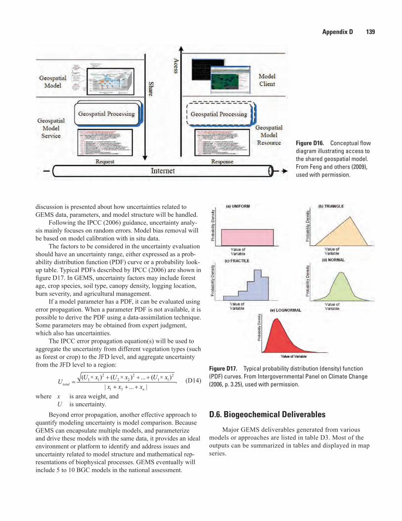
Consortium (OGC) Web Processing Service (WPS) standard (fig. D16).

Assessment results related to the evaluation of ecosys-tem services, such as soil erosion and deposition, biomass production, CO2 emission, and GHG flux, will be evaluated and distributed using the model-sharing platform (fig. D15). For a specific region and specific interest, however, numer-ous submodels can be added to reflect the relative effective-ness and efficiency of management activities. For example, water quantity and water quality, which are important indices of ecosystem services, are increasingly affected by natural and anthropogenic activities. The widely used Soil and Water Assessment Tool (SWAT) can be used to estimate the land-phase processes (for example, surface runoff, soil erosion, nonpoint-source nutrient loss, groundwater recharge, and baseflow) and water-phase processes (for example, water routing, sediment transport, and nutrient transport and its fate in the aquatic systems). GEMS will link with SWAT to assess the climate-change effects on water availability, and sediment and nutrient transport for the landscape. A pilot platform, named EcoServ (ecosystems services model), was developed in the Prairie Pothole region (PPR) to simulate the diversity of ecosystem services simultaneously at landscape scale.

D.5. Estimating Uncertainties

Uncertainty estimates can be in the form of estimated percent errors, standard deviations, confidence intervals, or any other relevant coefficient (Larocque and others, in press). For the assessment, an overall approach to assessing uncer-tainties is presented in appendix G of this report. Here, a brief

Figure D15. Diagram showing the system structure of the Geospatial Model Sharing Platform. From Feng and others (2009), used with permission. Abbreviations are found in the Abbreviations, Acronyms, and Chemical Symbols listing in the front of this report.

Appendix D 139

discussion is presented about how uncertainties related to GEMS data, parameters, and model structure will be handled.

Following the IPCC (2006) guidance, uncertainty analy-sis mainly focuses on random errors. Model bias removal will be based on model calibration with in situ data.

The factors to be considered in the uncertainty evaluation should have an uncertainty range, either expressed as a prob-ability distribution function (PDF) curve or a probability look-up table. Typical PDFs described by IPCC (2006) are shown in figure D17. In GEMS, uncertainty factors may include forest age, crop species, soil type, canopy density, logging location, burn severity, and agricultural management.

If a model parameter has a PDF, it can be evaluated using error propagation. When a parameter PDF is not available, it is possible to derive the PDF using a data-assimilation technique. Some parameters may be obtained from expert judgment, which also has uncertainties.

The IPCC error propagation equation(s) will be used to aggregate the uncertainty from different vegetation types (such as forest or crop) to the JFD level, and aggregate uncertainty from the JFD level to a region:

, (D14)

where x is area weight, and U is uncertainty.

Beyond error propagation, another effective approach to quantify modeling uncertainty is model comparison. Because GEMS can encapsulate multiple models, and parameterize and drive these models with the same data, it provides an ideal environment or platform to identify and address issues and uncertainty related to model structure and mathematical rep-resentations of biophysical processes. GEMS eventually will include 5 to 10 BGC models in the national assessment.

D.6. Biogeochemical Deliverables

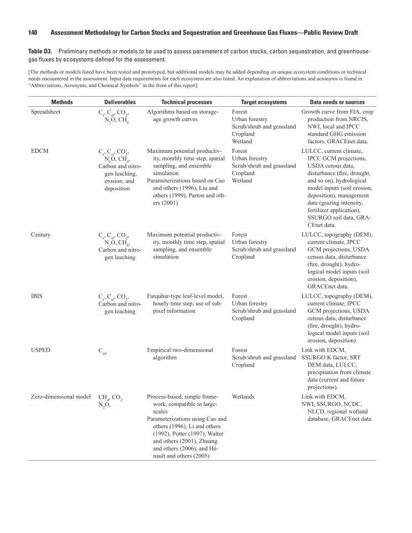
Major GEMS deliverables generated from various models or approaches are listed in table D3. Most of the outputs can be summarized in tables and displayed in map series.

Figure D16. Conceptual flow diagram illustrating access to the shared geospatial model. From Feng and others (2009), used with permission.

Figure D17. Typical probability distribution (density) function (PDF) curves. From Intergovernmental Panel on Climate Change (2006, p. 3.25), used with permission.


Table D3. Preliminary methods or models to be used to assess parameters of carbon stocks, carbon sequestration, and greenhouse-gas fluxes by ecosystems defined for the assessment.

[The methods or models listed have been tested and prototyped, but additional models may be added depending on unique ecosystem conditions or technical needs encountered in the assessment. Input data requirements for each ecosystem are also listed. An explanation of abbreviations and acronyms is found in “Abbreviations, Acronyms, and Chemical Symbols” in the front of this report]

Methods Deliverables Technical processes Target ecosystems Data needs or sources

Spreadsheet Cs, Csr, CO2, N2O, CH4

Algorithms based on storage-age growth curves

ForestUrban forestryScrub/shrub and grasslandCroplandWetland

Growth curve from FIA, crop production from NRCIS, NWI, local and IPCC standard GHG emission factors, GRACEnet data.

EDCM Cs, Csr, CO2, N2O, CH4,

Carbon and nitro-gen leaching, erosion, and deposition

Maximum potential productiv-ity, monthly time step, spatial sampling, and ensemble simulation

Parameterizations based on Cao and others (1996), Liu and others (1999), Parton and oth-ers (2001)

ForestUrban forestryScrub/shrub and grasslandCroplandWetland

LULCC, current climate, IPCC GCM projections, USDA census data, disturbance (fire, drought, and so on), hydrological model inputs (soil erosion, deposition), management data (grazing intensity, fertilizer application), SSURGO soil data, GRA-CEnet data.

Century Cs, Csr, CO2, N2O, CH4,

Carbon and nitro-gen leaching

Maximum potential productiv-ity, monthly time step, spatial sampling, and ensemble simulation

ForestUrban forestryScrub/shrub and grasslandCropland

LULCC, topography (DEM), current climate, IPCC GCM projections, USDA census data, disturbance (fire, drought), hydro-logical model inputs (soil erosion, deposition), GRACEnet data.

IBIS Cs, Csr, CO2,Carbon and nitro-

gen leaching

Farquhar-type leaf-level model, hourly time step, use of sub-pixel information

ForestUrban forestryScrub/shrub and grasslandCropland

LULCC, topography (DEM), current climate, IPCC GCM projections, USDA census data, disturbance (fire, drought), hydro-logical model inputs (soil erosion, deposition).

USPED CedEmpirical two-dimensional

algorithmForestScrub/shrub and grasslandCropland

Link with EDCM,SSURGO K factor, SRT

DEM data, LULCC, precipitation from climate data (current and future projections).

Zero-dimensional model CH4, CO2N2O,

Process-based, simple frame-work, compatible in large-scales

Parameterizations using Cao and others (1996), Li and others (1992), Potter (1997), Walter and others (2001), Zhuang and others (2006), and Hé-nault and others (2005)

Wetlands Link with EDCM,NWI, SSURGO, NCDC,

NLCD, regional wetland database, GRACEnet data.

Appendix D 141

D.7. References Cited

[Reports that are only available online may require a subscription for access.]

Avissar, Roni, 1992, Conceptual aspects of a statistical-dynamical approach to represent landscape subgrid-scale heterogeneities in atmospheric models: Journal of Geophysical Research, v. 97, no. D3, p. 2729–2742, doi:10.1029/91JD01751.

Cao, Mingkui, Marshall, Stewart, and Gregson, Keith, 1996, Global carbon exchange and methane emissions from natural wetlands—Application of a process-based model: Journal of Geophysical Research, v. 101, no. D9, p. 14399–14414, doi:10.1029/96JD00219.

Chen, J.M., Ju, Weimin, Cihlar, Josef, Price, David, Liu, Jane, Chen, Wenjun, Pan, Jianjun, Black, Andy, and Barr, Alan, 2003, Spatial distribution of carbon sources and sinks in Canada’s forests: Tellus B, v. 55, no. 2, p. 622–641, doi:10.1034/j.1600-0889.2003.00036.x.

Chen, M., Liu, S., and Tieszen, L., 2006, State-parameter esti-mation of ecosystem models using a Smoothed Ensemble Kalman Filter, in Voinov, A., Jakeman, A.J., and Rizzoli, A.E., eds., Proceedings of the iEMSs third biennial meet-ing—Summit on environmental modeling and software: Burlington, Vt., International Environmental Modelling and Software Society, 7 p. on one CD-ROM., accessed June 18, 2010, at http://www.iemss.org/iemss2006/papers/w16/334_Chen_1.pdf.

Chen, M., Liu, S., Tieszen, L.L., and Hollinger, D.Y., 2008, An improved state-parameter analysis of ecosystem models using data assimilation: Ecological Modelling, v. 219, no. 3–4, p. 317–326, accessed June 18, 2010, at http://dx.doi.org/10.1016/j.ecolmodel.2008.07.013.

Chen, Wenjun, Chen, Jing, and Cihlar, Josef, 2000, An inte-grated terrestrial ecosystem carbon-budget model based on changes in disturbance, climate, and atmospheric chemistry: Ecological Modelling, v. 135, no. 1, p. 55–79, doi:10.1016/S0304-3800(00)00371-9.

Conrad, R., 1989, Control of methane production in terrestrial ecosystems, in Andreae, M.O., and Schimel, D.S., eds., Exchange of trace gases between terrestrial ecosystems and the atmosphere: New York, John Wiley and Sons, p. 39–58.

Evensen, Geir, 1994, Sequential data assimilation with a non-linear quasi-geostrophic model using Monte Carlo methods to forecast error statistics: Journal of Geophysical Research, v. 99, no. C5, p. 10143–10162, doi:10.1029/94JC00572.

Evensen, Geir, 2003, The ensemble Kalman filter—Theo-retical formulation and practical implementation: Ocean Dynamics, v. 53, no. 4, p. 343–367, doi:10.1007/s10236-003-0036-9.

Farquhar, G.D., von Caemmerer, Susanne, and Berry, J.A., 1980, A biochemical model of photosynthetic CO2 assimi-lation in leaves of C3 species: Planta, v. 149, p. 78–90, doi:10.1007/BF00386231.

Feng, Min, Liu, Shuguang, Ned, H.E., Jr., and Yin, Fang, 2009, Distributed geospatial model sharing based on open interoperability standards: Journal of Remote Sensing, v. 13, no. 6, p. 1060–1066.

Fitz, H.C., and Hughes, N., 2008, Wetland ecological mod-els: Gainesville, Fla., University of Florida, Institute of Food and Agricultural Sciences Extension SL257, 6 p., accessed June 18, 2010, at http://edis.ifas.ufl.edu/pdffiles/SS/SS48100.pdf.

Foley, J.A., Prentice, I.C., Ramankutty, Navin, Levis, Samuel, Pollard, David, Sitch, Steven, and Haxeltine, Alex, 1996, An integrated biosphere model of land surface process, terrestrial carbon balance, and vegetation dynamics: Global Biogeochemical Cycles, v. 10, no. 4, p. 603–628.

Hénault, C., Bizouard, F., Laville, P., Gabrielle, B., Nicoul-laud, B., Germon, J.C., and Cellier, P., 2005, Predicting in situ soil N2O emission using NOE algorithm and soil database: Global Change Biology, v. 11, no. 1, p. 115–127, doi:10.1111/j.1365-2486.2004.00879.x.

Houghton, R.A., Hackler, J.L., and Lawrence, K.T., 1999, The U.S. carbon budget—Contributions from land-use change: Science, v. 285, no. 5427, p. 574–578, doi:10.1126/sci-ence.285.5.

Huang, Chengquan, Goward, S.N., Masek, J.G., Gao, Feng, Vermote, E.F., Thomas, Nancy, Schleeweis, Karen, Ken-nedy, R.E., Zhu, Zhiliang, Eidenshink, J.C., and Town-shend, J.R.G., 2009, Development of time series stacks of Landsat images for reconstructing forest disturbance history: International Journal of Digital Earth, v. 2, no. 3, p. 195–218, doi:10.1080/17538940902801614.

Intergovernmental Panel on Climate Change, 1997, Revised 1996 IPCC guidelines for national greenhouse gas inven-tories: Paris, International Panel on Climate Change, 3 v., accessed June 18, 2010, at http://www.ipcc-nggip.iges.or.jp/public/gl/invs1.html.)

Intergovernmental Panel on Climate Change, 2006, 2006 IPCC guidelines for national greenhouse gas inventories (Prepared by the IPCC National Greenhouse Gas Inven-tories Programme; edited by H.S. Eggleston, L. Buendia, K. Miwa, T. Ngara, and K. Tanabe): Hayama, Kanagawa, Japan, Institute for Global Environmental Strategies, 5 v., accessed June 14, 2010, at http://www.ipcc-nggip.iges.or.jp/public/2006gl/index.html.

Kimball, J.S., Running, S.W., and Saatchi, S.S., 1999, Sensi-tivity of boreal forest regional water flux and net primary production simulations to sub-grid scale land cover com-

http://dx.doi.org/10.1016/j.ecolmodel.2008.07.013



plexity: Journal of Geophysical Research, v. 104, no. D22, p. 27789–27801.

Lal, Rattan, Griffin, Michael, Apt, Jay, Lave, Lester, and Mor-gan, M.G., 2004, Managing soil carbon: Science, v. 304, no. 5669, p. 393.

Larocque, G.R., Bhatti, J.S., Ascough, J.C., II, Liu, J., Luckai, N., Mailly, D., Archambault, L., and Gordon, A.M., in press, An analytical framework to assist decision makers in the use of forest ecosystem model predictions: Envi-ronmental Modelling & Software, doi:10.1016/j.env-soft.2010.03.009, corrected proof accessed June 18, 2010, at http://dx.doi.org/10.1016/j.envsoft.2010.03.009.

Li, Changsheng, Frolking, Steve, and Frolking, T.A., 1992, A model of nitrous oxide evolution from soil driven by rainfall events—1. Model structure and sensitivity: Journal of Geo-physical Research, v. 97, no. D9, p. 9759–9776.

Liu, Jinxun, Liu, Shuguang, and Loveland, T.R., 2006, Temporal evolution of carbon budgets of the Appa-lachian forests in the U.S. from 1972 to 2000: Forest Ecology and Management, v. 222, no. 1–3, p. 191–201, doi:10.1016/j.foreco.2005.09.028.

Liu, Jinxun, Liu, Shuguang, Loveland, T.R., and Tieszen, L.L., 2008, Integrating remotely sensed land cover observations and a biogeochemical model for estimating forest ecosys-tem carbon dynamics: Ecological Modelling, v. 219, no. 3-4, p. 361–372.

Liu, Jinxun, Price, D.T., and Chen, J.M., 2005, Nitrogen con-trols on ecosystem carbon sequestration—A model imple-mentation and application to Saskatchewan, Canada: Eco-logical Modelling, v. 186, no. 2, p. 178–195, doi:10.1016/jecolmodel.2005.01.036.

Liu, S., Kaire, M., Wood, E., Diallo, O., and Tieszen, L.L., 2004, Impacts of land use and climate change on car-bon dynamics in south-central Senegal: Journal of Arid Environments, v. 59, no. 3, p. 583–604, doi:10.1016/jaridenv.2004.03.023.

Liu, Shuguang, Anderson, Pamela, Zhou, Guoyi, Kauffman, Boone, Hughes, Flint, Schimel, David, Watson, Vicente, and Tosi, Joseph, 2008, Resolving model parameter values from carbon and nitrogen stock measurements in a wide range of tropical mature forests using nonlinear inversion and regression trees: Ecological Modelling, v. 219, no. 3–4, p. 327–341, accessed June 18, 2010, at http://dx.doi.org/10.1016/j.ecolmodel.2008.07.025.

Liu, Shuguang, Bliss, Norman, Sundquist, Eric, and Hunting-ton, T.G., 2003, Modeling carbon dynamics in vegetation and soil under the impact of soil erosion and deposition: Global Biogeochemical Cycles, v. 17, no. 2, p. 1074, doi:10.1029/2002GB002010.

Liu, Shuguang, Loveland, T.R., and Kurtz, R.M., 2004, Contemporary carbon dynamics in terrestrial ecosystems in the southeastern plains of the United States: Environ-mental Management, v. 33, Supplement 1, p. S442–S456, doi:10.1007/s00267-003-9152-z.

Liu, Shuguang, Reiners, W.A., Keller, Michael, and Schimel, D.S., 1999, Model simulation of changes in N2O and NO emissions with conversion of tropical rain forests to pastures in the Costa Rican Atlantic zone: Global Biogeo-chemical Cycles, v. 13, p. 663–677.

McGuire, A.D., Sitch, S., Clein, J.S., Dargaville, R., Esser, G., Foley, J., Heimann, M., Joos, F., Kaplan, J., Kicklighter, D.W., Meier, R.A., Melillo, J.M., Moore, B., Prentice, I.C., Ramankutty, N., Reichenau, T., Schloss, A., Tian, H., Wil-liams, L.J., and Wittenberg, U., 2001, Carbon balance of the terrestrial biosphere in the twentieth century; Analyses of CO2, climate and land use effects with four process-based ecosystem models: Global Biogeochemical Cycles, v. 15, no. 1, p. 183–206, doi:10.1029/2000GB001298.

McGuire, A.D., Wirth, C., Apps, M., Beringer, J., Clein, J., Epstein, H., Kicklighter, D.W., Bhatti, J., Chapin, F.S.I., de Groot, B., Efremov, D., Eugster, W., Fukuda, M., Gower, T., Hinzman, L., Huntley, B., Jia, G.J., Kasischke, E., Melillo, J., Romanovsky, V., Shvidenko, A., Vaganov, E., and Walker, D., 2002, Environmental variation, vegetation distribution, carbon dynamics and water/energy exchange at high latitudes: Journal of Vegetation Science, v. 13, no. 3, p. 301–314.

Melillo, J.M., Borchers, J., Chaney, J., Fisher, H., Fox, S., Haxeltine, A., Janetos, A., Kicklighter, D.W., Kittel, T.G.F., Mcguire, A.D., McKeown, R., Neilson, R., Nemani, R., Ojima, D.S., Painter, T., Pan, Y., Parton, W.J., Pierce, L., Pitelka, L., Prentice, C., Rizzo, B., Rosenbloom, N.A., Run-ning, S., Schimel, D.S., Sitch, S., Smith, T., and Woodward, I., 1995, Vegetation ecosystem modelling and analysis project—Comparing biogeography and biogeochemistry models in a continental-scale study of terrestrial ecosystem responses to climate-change and CO2 doubling: Global Bio-geochemical Cycles, v. 9, no. 4, p. 407–437.

Metherell, A.K., Harding, L.A., Cole, C.V., and Parton, W.J., 1993, Century soil organic matter model environment; Technical documentation; Agroecosystem version 4.0: U.S. Department of Agriculture, Agricultural Research Service, Great Plains System Research Unit Technical Report 4, accessed June 18, 2010, at http://daac.ornl.gov/data/model_archive/CENTURY/century_vemap_m4/comp/Century_Users_Manual_V4.pdf.

Mitas, Lubos, and Mitasova, Helena, 1998, Distributed soil erosion simulation for effective erosion preven-tion: Water Resources Research, v. 34, no. 3, p. 505–516, doi:10.1029/97WR03347.



Appendix D 143

Pan, Yude, Melillo, J.M., McGuire, A.D., Kicklighter, D.W., Pitelka, L.F., Hibbard, Kathy, Pierce, L.L., Running, S.W., Ojima, D.S., Parton, W.J., and Schimel, D.S., 1998, Modelled responses of terrestrial ecosystems to elevated atmospheric CO2—A comparison of simulations by the biogeochemistry models of the Vegetation/Ecosystem Modelling and Analysis Project (Vemap): Oecologia, v. 114, p. 389–404.

Parton, W.J., Gutmann, M.P., Williams, S.A., Easter, Mark, and Ojima, Dennis, 2005, Ecological impact of histori-cal land-use patterns in the Great Plains; A methodologi-cal assessment: Ecological Applications, v. 15, no. 6, p. 1915–1928, doi:10.1890/04-1392.

Parton, W.J., Holland, E.A., Del Grosso, S.J., Hartman, M.D., Martin, R.E., Mosier, A.R., Ojima, D.S., and Schimel, D.S., 2001, Generalized model for NOx and N2O emissions from soils: Journal of Geophysical Research, v. 106, no. D15, p. 17403–17419, doi:10.1029/2001JD900101.

Parton, W.J., Schimel, D.S., Cole, C.V., and Ojima, D.S., 1987, Analysis of factors controlling soil organic-matter levels in Great-Plains grasslands: Soil Science Society of America Journal, v. 51, p. 1173–1179.

Parton, W.J., Scurlock, J.M.O., Ojima, D.S., Gilmanov, T.G., Scholes, R.J., Schimel, D.S., Kirchner, T., Menaut, J.-C., Seastedt, T., Garcia Moya, E., Kamnalrut, A., and Kin-yamario, J.I., 1993, Observations and modeling of biomass and soil organic matter dynamics for the grassland biome worldwide: Global Biogeochemical Cycles, v. 7, no. 4, p. 785–809.

Peng, Changhui, Liu, Jinxun, Dang, Qinglai, Zhou, Xiaolu, and Apps, Mike, 2002, Developing carbon-based ecologi-cal indicators to monitor sustainability of Ontario’s forests: Ecological Indicators, v. 1, no. 4, p. 235–246, doi:10.1016/S1470-160X(02)00010-9.

Pierce, L.L., and Running, S.W., 1995, The effects of aggre-gating sub-grid land surface variation on large-scale esti-mates of net primary production: Landscape Ecology, v. 10, no. 4, p. 239–253.

Potter, C.S., 1997, An ecosystem simulation model for methane production and emission from wetlands: Global Biogeochemical Cycles, v. 11, no. 4, p. 495–506, doi:10.1029/97GB02302.

Potter, C., Klooster, S., Tan, P., Steinbach, M., Kumar, V., and Genovese, V., 2005, Variability in terrestrial carbon sinks over two decades; Part 2, Eurasia: Global and Planetary Change, v. 49, p. 177–186.

Potter, C.S., Randerson, J.T., Field, C.B., Matson, P.A., Vitousek, P.M., Mooney, H.A., and Klooster, S.A., 1993, Terrestrial ecosystem production—A process model based on global satellite and surface data: Global Biogeochemical Cycles, v. 7, no. 4, p. 811–841, doi:10.1029/93GB02725.

Reiners, W.A., Liu, S., Gerow, K.G., Keller, M., and Schimel, D.S., 2002, Historical and future land use effects on N2O and NO emissions using an ensemble model-ling approach; Costa Rica’s Caribbean lowlands as an example: Global Biogeochemical Cycles, v. 16, no. 4, doi:10.1029/2001GB001437.

Reinhardt, E.D., Keane, R.E., and Brown, J.K., 1997, First order fire effects model; FOFEM 4.0 user’s guide: U.S. Department of Agriculture, Forest Service, Intermountain Research Station General Technical Report INT–GTR–344, 65 p., accessed June 14, 2010, at http://www.fs.fed.us/rm/pubs_int/int_gtr344.html.

Running, S.W., and Coughlan, J.C., 1988, General model of forest ecosystem processes for regional applications, I. Hydrologic balance, canopy gas exchange and primary pro-duction processes: Ecological Modelling, v. 42, p. 125–154.

Schimel, D.S., Braswell, B.H., Holland, E.A., McKeown, Rebecca, Ojima, D.S., Painter, T.H., Parton, W.J., and Townsend, A.R., 1994, Climatic, edaphic, and biotic controls over storage and turnover of carbon in soils: Global Biogeochemical Cycles, v. 8, no. 3, p. 279–293, doi:10.1029/94GB00993.

Sierra, C.A., Loescher, H.W., Harmon, M.E., Richardson, A.D., Hollinger, D.Y., and Perakis, S.S., 2009, Interannual variation of carbon fluxes from three contrasting evergreen forests—The role of forest dynamics and climate: Ecology, v. 90, no. 10, p. 2711–2723, doi:10.1890/08-0073.1.

Skog, K.E., 2008, Sequestration of carbon in harvested wood products for the United States: Forest Products Journal, v. 58, no. 6, p. 56–72.

Skog, K.E., and Nicholson, G.A., 1998, Carbon cycling through wood products—The role of wood and paper prod-ucts in carbon sequestration: Forest Products Journal, v. 48, p. 75–8

Smith, J.E., Heath, L.S., Skog, K.E., and Birdsey, R.A., 2006, Methods for calculating forest ecosystem and harvested carbon with standard estimates for forest types of the United States: U.S. Department of Agriculture, Forest Service, Northeastern Research Station General Technical Report NE–343, 216 p.

Tan, Zhengxi, Liu, Shuguang, Johnston, C.A., Loveland, T.R., Tieszen, L.L., Liu, Jinxun, and Kurtz, Rachel, 2005, Soil organic carbon dynamics as related to land use history in the Northwestern Great Plains: Global Biogeochemical Cycles, v. 19, doi:10.1029/2005GB002536.

Turner, D.P., Cohen, W.B., and Kennedy, R.E., 2000, Alterna-tive spatial resolutions and estimation of carbon flux over a managed forest landscape in western Oregon: Landscape Ecology, v. 15, p. 441–452.

http://www.fs.fed.us/rm/pubs_int/int_gtr344.html




Turner, D.P., Dodson, Rusty, and Marks, Danny, 1996, Com-parison of alternative spatial resolutions in the application of a spatially distributed biogeochemical model over com-plex terrain: Ecological Modelling, v. 90, no. 1, p. 53–67, doi:10.1016/0304-3800(95)00143-3.

U.S. Congress, 2007, Energy Independence and Secu-rity Act—Public Law 110–140: U.S. Congress, 311 p., available at http://frwebgate.access.gpo.gov/cgi-bin/getdoc.cgi?dbname=110_cong_public_laws&docid=f:publ140.110.pdf.

Walter, B.P., Heilmann, Martin, and Matthews, Elaine, 2001, Modeling modern methane emissions from natu-ral wetlands, 1. Model description and results: Journal of Geophysical Research, v. 106, no. D24, p. 34189–34206, doi:10.1029/2001JD900165.

Yuan, Wenping, Liu, Shuguang, Zhou, Guangsheng, Zhou, Guoyl, Tieszen, L.L., Baldocchi, Dennis, Bernhofer, Christian, Gholz, Henry, Goldstein, A.H., Goulden, M.L.,

Hollinger, D.Y., Hu, Yueming, Law, B.E., Stoy, P.C., Vesala, Timo, and Wofsy, S.C., 2007, Deriving a light use effi-ciency model from eddy covariance flux data for predicting daily gross primary production across biomes: Agricul-tural and Forest Meteorology, v. 143, no. 3–4, p. 189–207, doi:10.1016/j.agrformet.2006.12.001.

Zhao, Shuqing, Liu, Shuguang, Li, Zhengpeng, and Sohl, T.L., 2010, Federal land management, carbon sequestration, and climate change in the southeastern U.S.—A case study with Fort Benning: Environmental Science and Technology, v. 44, no. 3, p. 992–997, doi:10.1021/es9009019.

Zhuang, Qianli, Melillo, J.M., Sarofim, M.C., Kicklighter, D.W., McGuire, A.D., Felzer, B.S., Sokolov, Andrei, Prinn, R.G., Steudler, P.A., and Hu, Shaomin, 2006, CO2 and CH4 exchanges between land ecosystems and the atmosphere in northern high latitudes over the 21st century: Geo-physical Research Letters, v. 33, p. L17403.1– L17403.5, doi:10.1029/2006GL026972.

Date post:	15-May-2018
Category:	Documents
Upload:	dodat
View:	219 times
Download:	2 times

Appendix D. Methods for Assessing Carbon Stocks, … D 123 Appendix D. Methods for Assessing Carbon...

Documents