247
APPENDIX E.1 2014 Model Guidelines Table of Contents

APPENDIX E.1
2014 Model Guidelines Table of Contents

City of Toronto InfoWorks CS Basement Flooding Model Studies
Guideline
Version 1.02 – October 2014

DRAFT CITY OF TORONTO INFOWORKS CS BASEMENT FLOODING MODEL STUDIES GUIDELINE Version 1.02 - October 2014
Table of Contents
VERSION CONTROL .................................................................................................................. V
ABBREVIATIONS ....................................................................................................................... VI
GLOSSARY OF COMMON TERMS ........................................................................................... VII
1.0 INTRODUCTION ...........................................................................................................1.1 1.1 PURPOSE AND INTENT .................................................................................................... 1.1
2.0 DATA COLLECTION .....................................................................................................2.1 2.1 DESKTOP COLLECTION .................................................................................................. 2.1
2.1.1 Base GIS Layers ............................................................................................ 2.1 2.1.2 Sewer Asset Geodatabase ........................................................................ 2.1 2.1.3 Operations and Maintenance Data ........................................................ 2.2 2.1.4 Flow Monitoring Information ...................................................................... 2.2 2.1.5 Other Supporting Data ............................................................................... 2.2
2.2 FIELD SURVEY .................................................................................................................. 2.3 2.2.1 Address Survey ............................................................................................. 2.3 2.2.2 Catchbasin Survey ...................................................................................... 2.3 2.2.3 Maintenance Hole Cover Survey .............................................................. 2.4 2.2.4 Low Point Survey .......................................................................................... 2.4 2.2.5 Outfall/Surface Drainage Structure Survey .............................................. 2.4 2.2.6 Resident Questionnaire ............................................................................... 2.5 2.2.7 Field Chamber/Facility Inspections ........................................................... 2.5
3.0 DATA ASSESSMENT AND GAP ANALYSIS ...................................................................3.1 3.1 DATA QUALITY ASSESSMENT .......................................................................................... 3.1
3.1.1 Asset Data Coverage ................................................................................. 3.1 3.1.2 Asset Data Gaps .......................................................................................... 3.2 3.1.3 Flow Monitoring and Rainfall Data............................................................ 3.2
3.2 ENGINEERING VALIDATION ........................................................................................... 3.2 3.3 DATA RECTIFICATION PROCEDURE AND DOCUMENTATION .................................... 3.4
3.3.1 Initial Asset Data Import into InfoWorks CS .............................................. 3.4 3.3.2 Data Rectification Procedure ................................................................... 3.5
4.0 INFOWORKS FILE MANAGEMENT AND SET-UP ...........................................................4.1 4.1 VERSIONING ................................................................................................................... 4.1 4.2 CATCHMENT GROUP HIERARCHY ................................................................................ 4.1 4.3 NETWORK MANAGEMENT ............................................................................................. 4.2 4.4 MODEL GROUP MANAGEMENT ................................................................................... 4.2 4.5 NAMING CONVENTIONS ............................................................................................... 4.4
4.5.1 EA Stage - Model Build ............................................................................... 4.5 4.5.2 Detailed Design Stage ................................................................................ 4.7 4.5.3 Development Application Review............................................................ 4.8
i

DRAFT CITY OF TORONTO INFOWORKS CS BASEMENT FLOODING MODEL STUDIES GUIDELINE Version 1.02 - October 2014
4.6 DATA FLAGGING ........................................................................................................... 4.9 4.7 SIMULATION PARAMETERS ........................................................................................... 4.10
4.7.1 Time Step Selection ................................................................................... 4.10 4.7.2 Simulation Parameter Defaults ................................................................ 4.10
4.8 ELEMENT DOCUMENTATION ....................................................................................... 4.11 4.9 MODEL VISUALIZATION STANDARDS .......................................................................... 4.12
4.9.1 Coordinate System .................................................................................... 4.12 4.9.2 Network Objects ........................................................................................ 4.14 4.9.3 Results Themes ........................................................................................... 4.14 4.9.4 Profile “Long-Section” View ..................................................................... 4.15
5.0 HYDRAULICS (CONVEYANCE MODELLING) ..............................................................5.1 5.1.1 Dual Drainage Principle .............................................................................. 5.1 5.1.2 Overland Flow Paths ................................................................................... 5.2 5.2.1 Node Definition ............................................................................................ 5.4 5.2.2 Manhole Flood Type ................................................................................... 5.5 5.3.1 Solution Model ........................................................................................... 5.18 5.3.2 Underground Pipe Cross-Sections ........................................................... 5.18 5.3.3 Minor Losses ................................................................................................ 5.19
5.4 OVERLAND MAJOR SYSTEM CONDUITS .................................................................... 5.20 5.4.2 Overland Spills at Low Points .................................................................... 5.22
5.5 ROOFS ........................................................................................................................... 5.23 5.5.1 Modelling Roofs- Physical Representation ............................................. 5.23 5.5.2 Modelling Large Parking Lots (ICI) ........................................................... 5.27 5.5.3 Modelling Reverse Driveways .................................................................. 5.28 5.5.4 Modelling Rear Yards ................................................................................ 5.28
5.6 SPECIAL HYDRAULIC STRUCTURES .............................................................................. 5.28 5.6.1 Weirs ............................................................................................................ 5.28 5.6.2 Orifices ........................................................................................................ 5.29 5.6.3 Sluice Gates ............................................................................................... 5.29 5.6.4 User-Control ................................................................................................ 5.30 5.6.5 Pumps .......................................................................................................... 5.30 5.6.6 Culverts ....................................................................................................... 5.31 5.6.7 Real Time Control ...................................................................................... 5.32
5.7 BOUNDARY CONDITIONS ............................................................................................ 5.32 5.7.1 Level Based ................................................................................................ 5.32 5.7.2 Flow Based .................................................................................................. 5.33
6.0 HYDROLOGY (SEWAGE AND RUNOFF MODELLING) .................................................6.1 6.1 OVERVIEW ....................................................................................................................... 6.1 6.2 SUBCATCHMENT SET-UP ................................................................................................. 6.2
6.2.1 Sanitary System ............................................................................................ 6.5 6.2.2 Storm/Combined System ........................................................................... 6.6 6.2.3 Roof Areas .................................................................................................... 6.8 6.2.4 Large Parking Lots, Reverse Driveways & Rear Yards ............................. 6.8
ii

DRAFT CITY OF TORONTO INFOWORKS CS BASEMENT FLOODING MODEL STUDIES GUIDELINE Version 1.02 - October 2014
6.3 DRY WEATHER FLOW ...................................................................................................... 6.9 6.3.1 EA Modelling ................................................................................................ 6.9 6.3.2 Development Reviews ................................................................................ 6.9
6.4 WET WEATHER FLOW ...................................................................................................... 6.9 6.4.1 Storm Runoff Surfaces ................................................................................. 6.9 6.4.2 Sanitary Infiltration and Inflow .................................................................. 6.12
7.0 CALIBRATION, VALIDATION AND PERFORMANCE ANALYSIS .................................7.13 7.1 CALIBRATIONS .............................................................................................................. 7.13
7.1.1 Dry Weather Flow ...................................................................................... 7.13 7.1.2 Sanitary Wet Weather Flow ...................................................................... 7.14 7.1.3 Storm Flow................................................................................................... 7.15
7.2 EXTREME STORM VALIDATION .................................................................................... 7.15 7.2.1 Historic Rainfall Events ............................................................................... 7.15 7.2.2 Long-Term Historic Data ........................................................................... 7.16
7.3 PERFORMANCE ANALYSIS ........................................................................................... 7.16 7.3.1 Model Stability ............................................................................................ 7.18
8.0 FLOODING IMPROVEMENT WORKS DEFINITION ........................................................8.1 8.1 CONVEYANCE IMPROVEMENTS ................................................................................... 8.1
8.1.1 Catchbasins ................................................................................................. 8.1 8.1.2 Underground Pipes ...................................................................................... 8.1
8.2 STORAGE IMPROVEMENTS ............................................................................................ 8.2 8.2.1 Underground - In-line Storage ................................................................... 8.2 8.2.2 Underground - Off-line Storage ................................................................. 8.3 8.2.3 Surface Storage Pond ................................................................................. 8.3 8.2.4 Design Sensitivity Analysis ........................................................................... 8.4
9.0 COMPLETED MODEL APPLICATIONS ...........................................................................9.1 9.1 DESIGN AND CONSTRUCTION ...................................................................................... 9.1 9.2 DEVELOPMENT REVIEWS ................................................................................................ 9.1
10.0 FINAL DELIVERABLES .................................................................................................10.1 10.1 MODEL SUBMISSIONS ................................................................................................... 10.1 10.2 MODEL RESULTS DOCUMENTATION ........................................................................... 10.2
10.2.1 Sewer Flow Model Results ......................................................................... 10.2 10.2.2 Overland Depth Model Results ................................................................ 10.3
10.3 MODEL DOCUMENTATION FOR FUTURE USERS ......................................................... 10.3 10.4 GEODATABASE SUBMISSION ....................................................................................... 10.3
iii
DRAFT CITY OF TORONTO INFOWORKS CS BASEMENT FLOODING MODEL STUDIES GUIDELINE Version 1.02 - October 2014
LIST OF APPENDICES
PROJECT SIGN-OFF SHEETS ...................................................................... A.1 APPENDIX A
HYDROLOGIC AND HYDRAULIC REFERENCES ......................................... B.1 APPENDIX BB.1 Hydrology ....................................................................................................................... B.1
B.1.1 Manning’s Roughness - Surface Flow ....................................................... B.1 B.1.2 Initial Abstraction ......................................................................................... B.1 B.1.3 Infiltration Parameters ................................................................................. B.2 B.1.4 Design Storm Events .................................................................................... B.2
B.2 Hydraulics ....................................................................................................................... B.6 B.2.1 Manning’s Roughness - Closed Conduit .................................................. B.6 B.2.2 Manning’s Roughness - Open Channel Conduits .................................. B.6 B.2.3 Weir Coefficients .......................................................................................... B.7 B.2.4 Minor Losses .................................................................................................. B.7 B.2.5 Culvert Parameters ...................................................................................... B.7
FLOW MONITORING ANALYTICAL PROCESSING ..................................... C.1 APPENDIX CC.1 Rain Gauge Network ................................................................................................... C.1 C.2 Data Analysis Approach ............................................................................................. C.2 C.3 Flow Monitoring Data Reporting ................................................................................ C.3
METADATA STRUCTURE ............................................................................. D.1 APPENDIX DD.1 Data Provided by the City ........................................................................................... D.1 D.2 Project Deliverables .................................................................................................... D.20
EXTERNAL RESOURCES ............................................................................... E.1 APPENDIX E
iv

APPENDIX E.2
Suggested Updates on 2014 Model Guideline
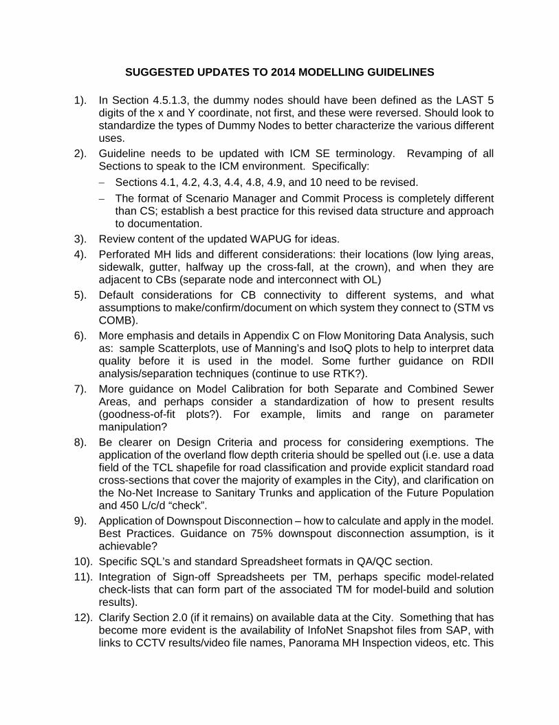
SUGGESTED UPDATES TO 2014 MODELLING GUIDELINES
1). In Section 4.5.1.3, the dummy nodes should have been defined as the LAST 5 digits of the x and Y coordinate, not first, and these were reversed. Should look to standardize the types of Dummy Nodes to better characterize the various different uses.
2). Guideline needs to be updated with ICM SE terminology. Revamping of all Sections to speak to the ICM environment. Specifically:
− Sections 4.1, 4.2, 4.3, 4.4, 4.8, 4.9, and 10 need to be revised.
− The format of Scenario Manager and Commit Process is completely different than CS; establish a best practice for this revised data structure and approach to documentation.
3). Review content of the updated WAPUG for ideas.
4). Perforated MH lids and different considerations: their locations (low lying areas, sidewalk, gutter, halfway up the cross-fall, at the crown), and when they are adjacent to CBs (separate node and interconnect with OL)
5). Default considerations for CB connectivity to different systems, and what assumptions to make/confirm/document on which system they connect to (STM vs COMB).
6). More emphasis and details in Appendix C on Flow Monitoring Data Analysis, such as: sample Scatterplots, use of Manning’s and IsoQ plots to help to interpret data quality before it is used in the model. Some further guidance on RDII analysis/separation techniques (continue to use RTK?).
7). More guidance on Model Calibration for both Separate and Combined Sewer Areas, and perhaps consider a standardization of how to present results (goodness-of-fit plots?). For example, limits and range on parameter manipulation?
8). Be clearer on Design Criteria and process for considering exemptions. The application of the overland flow depth criteria should be spelled out (i.e. use a data field of the TCL shapefile for road classification and provide explicit standard road cross-sections that cover the majority of examples in the City), and clarification on the No-Net Increase to Sanitary Trunks and application of the Future Population and 450 L/c/d “check”.
9). Application of Downspout Disconnection – how to calculate and apply in the model. Best Practices. Guidance on 75% downspout disconnection assumption, is it achievable?
10). Specific SQL’s and standard Spreadsheet formats in QA/QC section.
11). Integration of Sign-off Spreadsheets per TM, perhaps specific model-related check-lists that can form part of the associated TM for model-build and solution results).
12). Clarify Section 2.0 (if it remains) on available data at the City. Something that has become more evident is the availability of InfoNet Snapshot files from SAP, with links to CCTV results/video file names, Panorama MH Inspection videos, etc. This

has been extremely helpful in being thorough with the model-build, especially in combined areas where the system condition is poor… better than the idealized nature assumed in the model. So too, the ESM and LiDAR data should be spelled out along with other TWAG shapefiles that can facilitate easy definition of an Impervious Layer, something that should be mandatory (vs. sample areas applied based on similar land use)…the imperviousness is TOO sensitive to runoff peak to leave to estimates.
13). Consider to include some of the advanced options in ICM for documentation, visualization and simulation. One example is that there are several User Number/Text fields now available (vs. 5 in CS), offering more flexibility and transparency.
14). Consider having ONE model for all system types (i.e. storm and sanitary/combined in the same geoplan, and even in separated sewersheds), with guidance on how to interconnect the three systems and what to consider in relation to roof connections and resulting RTK methods (or other methods?).
15). Provide a more descriptive methodology and/or process for what to apply for private sites such as large parking lots and catchbasins in shopping malls and commercial properties.
16). Include a Section on Pump Stations
17). Include CSO performance analysis and evaluation guideline; include water quality modelling process/Best Practices for CSOs and Storm drainage systems.
18). Considerations for Boundary Conditions need to be expanded. Update and enhance the Boundary Conditions Section:
− Explanations for external Study Area overlap, including Future or Past study areas.
− When and how to apply TRCA HEC-RAS files? Limitations and best practices when using floodline data.
− Incorporating upstream and downstream storm, sanitary/combined trunk model flow and water levels.
19). How to simulate solutions in the model environment, include specific examples:
− Storage - inline, offline… what to consider (low flow channels, passive controls vs. automation using real time or conditional control settings, hydraulics, suitability)
− Best practices for simulating orifices, weirs etc.
− How/when to apply Water Quality solutions like Bioretention, Exfiltration, Wet Ponds in the model environment
20). Standardize the naming convention of the ID’s and Solution Types for EAs, and link to the new standard Geodatabase structure and ID’s being developed for BFPP implementation.
21). Transition from EA to Implementation Phase: grouping, bundling, and sequencing of recommended projects, what to consider when changing solutions, what needs to be presented to City/MOE, data and format for passing to the design and construction phase (e.g. geodatabase template, topographic data, cost-benefit

calculations, naming conventions, etc.); standardize the procedure and requirements.
22). Other uses of the Model? E.g. Development Applications – one of the issues is applying Design Sheet “steady state” hydraulic methodologies as compared to the InfoWorks “dynamic state” hydraulic environment, with respect to Rehabilitation projects and Development Application support
23). Replacement of Appendix D with new geodatabase requirements, directly affiliating with TWAG and InfoNet structure set-up.
24). Include some testing of methods to demonstrate sensitivity of parameters such as:
− CB efficiency or curve types
− Overland flow connectivity especially in combined systems where there are many storm/sanitary/combined nodes and gully/lid types
− Overland flow cross-sections and the sensitivity to application of the width parameter (vs. providing too many cross-section types)
− Methodology for representation and modelling of Ditches and Swales; ditch and swale drainage needs more discussion
− In ICM, Subcatchments can drain to other Sub-catchments, something that could be considered for modelling disconnected roofs
− Water quality simulation approaches, if it remains (more the physical manipulation of links/nodes and application of SUDS Module, not physically representing build-up/washoff or pollutants in the detailed models)
25). Specifications for the digital deliverables of the Infoworks model “iwc” files (e.g. final simulation model file with all job control and run time files such as rainfall, unit loading rates, direct inflow, and boundary condition files), with spreadsheets and template of the ICM Structure, etc.
26). Data Assessment and Data Gap Analysis:
− Too much “instructions” in this section
27). InfoWorks File Management and Set Up:
− Review and general edit
− There are more user field available in ICM
− Review/Update Flagging, include remarks
− Documentation for the validation/check /fix is confusing and too much. For example if an invert is Flagged as “inferred” then it already meant the original invert was missing or corrupt.
− Themes, etc. will need to be updated for ICM.
− Overland Flow Depth – this criteria is variable based on road width/lanes; documentation needs to be added on this criteria
− Ditch Performance – same as above, each one will be different.
− Use of “user controlled link” is problematic when dealing with the roof split. Needs to be updated. Instability issues caused by use of overland “user control link”. Develop an alternative to the roof flow split and investigate “splitting” the

rainfall thereby reducing the number of model elements. E.g., this can be modified by use of overland conduits instead of “user control link”.
28). Hydraulics
− Inlet curves do not seem to be consistent, update
− Update CB capture curves for High Capacity Inlets versus inlet capture curves for double honey combs and grid CBs; head discharge tables in the guideline are not consistent
− Research project idea – redo the experiment using scaled physical models, can use 3-D printing to “print” the inlets and set up a scale road with controlled flows – something different !
− Consideration for 2-D Modeling, and its application with Toronto’s GCC available data.
− Add some discussion on 2-D. E.g. Overland – 2D
29). Hydrology
− Is RTK still the way to go for sanitary?
− Is the Buffer the way to go for I/I area? “Parcel” makes more sense.
− Figures need to updated and clearer
30). Calibration, Validation and Performance Analysis
− May 12, 2000 rainfall data – small discrepancy in the hyetograph presented in the guideline vs the IW files provided; numbers seem to be missing; make sure the files and the tables are consistent with each other
− Re-visit calibration criteria: calibrating the Volume and Peak Flow are easier but matching Depth is difficult; review WAPUG specifications
− Performance analysis – need to update overland flow depth analysis
31). Flood Improvement Works Definition
− Review and general edit/update
32). Completed Model Applications
− Review and general edit/update
33). Final Deliverables
− Review and general edit/update
− More explanations in this section to define the deliverables/checklists.
− New section on “Thematic Maps”, profiles etc.
34). Use of Excel tool to generate overland cross-sections in ICM (user to input ROW width, road width, cross slope and height of overland channel)
35). Use of scatter graphs (depth vs velocity) for the purpose of calibration and flow data quality assessments
36). Discussion on different cases to represent various scenarios (Flat roof disconnected to large parking lot to sewers, etc.)
37). Develop SQLs to check adherence to modelling guidelines for reviewers
38). Consider use of Area Take off within InfoWorks to calculate impervious areas related to roads, roofs, other and pervious areas
39). Consider possible use of single model to represent calibration and validation
40). More details on representation of fully combined and partially combined sewers
41). Step by Step process for Calibration and Validation for different systems. Provide guidance on range of values to be modified for purpose of calibration.
42). Performing Sensitivity tests to account for spatial rainfall during calibration and validation versus radar rainfall data.
43). Guidance on representation of LIDs for water quality and to implement green street guidelines

APPENDIX E.3 – E.12
E.3 Cost-Benefitting properties calculations E.4 Modelling combined sewer areas E.5 Investigating and modelling dual manholes E.6 Modelling perforated manhole lids E.7 Modelling ditches, and incorporating ditches with the major system E.8 Application of climate change IDF curves E.9 Accounting for grease and sediments in sewers when developing solutions E.10 QA/QC requirements and check lists E.11 Set-up of Roofs in the Models

APPENDIX E.1
2014 Model Guidelines Table of Contents

APPENDIX E.2
Suggested Updates on 2014 Model Guideline

SUGGESTED UPDATES TO 2014 MODELLING GUIDELINES
1). In Section 4.5.1.3, the dummy nodes should have been defined as the LAST 5 digits of the x and Y coordinate, not first, and these were reversed. Should look to standardize the types of Dummy Nodes to better characterize the various different uses.
2). Guideline needs to be updated with ICM SE terminology. Revamping of all Sections to speak to the ICM environment. Specifically:
− Sections 4.1, 4.2, 4.3, 4.4, 4.8, 4.9, and 10 need to be revised.
− The format of Scenario Manager and Commit Process is completely different than CS; establish a best practice for this revised data structure and approach to documentation.
3). Review content of the updated WAPUG for ideas.
4). Perforated MH lids and different considerations: their locations (low lying areas, sidewalk, gutter, halfway up the cross-fall, at the crown), and when they are adjacent to CBs (separate node and interconnect with OL)
5). Default considerations for CB connectivity to different systems, and what assumptions to make/confirm/document on which system they connect to (STM vs COMB).
6). More emphasis and details in Appendix C on Flow Monitoring Data Analysis, such as: sample Scatterplots, use of Manning’s and IsoQ plots to help to interpret data quality before it is used in the model. Some further guidance on RDII analysis/separation techniques (continue to use RTK?).
7). More guidance on Model Calibration for both Separate and Combined Sewer Areas, and perhaps consider a standardization of how to present results (goodness-of-fit plots?). For example, limits and range on parameter manipulation?
8). Be clearer on Design Criteria and process for considering exemptions. The application of the overland flow depth criteria should be spelled out (i.e. use a data field of the TCL shapefile for road classification and provide explicit standard road cross-sections that cover the majority of examples in the City), and clarification on the No-Net Increase to Sanitary Trunks and application of the Future Population and 450 L/c/d “check”.
9). Application of Downspout Disconnection – how to calculate and apply in the model. Best Practices. Guidance on 75% downspout disconnection assumption, is it achievable?
10). Specific SQL’s and standard Spreadsheet formats in QA/QC section.
11). Integration of Sign-off Spreadsheets per TM, perhaps specific model-related check-lists that can form part of the associated TM for model-build and solution results).
12). Clarify Section 2.0 (if it remains) on available data at the City. Something that has become more evident is the availability of InfoNet Snapshot files from SAP, with links to CCTV results/video file names, Panorama MH Inspection videos, etc. This

has been extremely helpful in being thorough with the model-build, especially in combined areas where the system condition is poor… better than the idealized nature assumed in the model. So too, the ESM and LiDAR data should be spelled out along with other TWAG shapefiles that can facilitate easy definition of an Impervious Layer, something that should be mandatory (vs. sample areas applied based on similar land use)…the imperviousness is TOO sensitive to runoff peak to leave to estimates.
13). Consider to include some of the advanced options in ICM for documentation, visualization and simulation. One example is that there are several User Number/Text fields now available (vs. 5 in CS), offering more flexibility and transparency.
14). Consider having ONE model for all system types (i.e. storm and sanitary/combined in the same geoplan, and even in separated sewersheds), with guidance on how to interconnect the three systems and what to consider in relation to roof connections and resulting RTK methods (or other methods?).
15). Provide a more descriptive methodology and/or process for what to apply for private sites such as large parking lots and catchbasins in shopping malls and commercial properties.
16). Include a Section on Pump Stations
17). Include CSO performance analysis and evaluation guideline; include water quality modelling process/Best Practices for CSOs and Storm drainage systems.
18). Considerations for Boundary Conditions need to be expanded. Update and enhance the Boundary Conditions Section:
− Explanations for external Study Area overlap, including Future or Past study areas.
− When and how to apply TRCA HEC-RAS files? Limitations and best practices when using floodline data.
− Incorporating upstream and downstream storm, sanitary/combined trunk model flow and water levels.
19). How to simulate solutions in the model environment, include specific examples:
− Storage - inline, offline… what to consider (low flow channels, passive controls vs. automation using real time or conditional control settings, hydraulics, suitability)
− Best practices for simulating orifices, weirs etc.
− How/when to apply Water Quality solutions like Bioretention, Exfiltration, Wet Ponds in the model environment
20). Standardize the naming convention of the ID’s and Solution Types for EAs, and link to the new standard Geodatabase structure and ID’s being developed for BFPP implementation.
21). Transition from EA to Implementation Phase: grouping, bundling, and sequencing of recommended projects, what to consider when changing solutions, what needs to be presented to City/MOE, data and format for passing to the design and construction phase (e.g. geodatabase template, topographic data, cost-benefit

calculations, naming conventions, etc.); standardize the procedure and requirements.
22). Other uses of the Model? E.g. Development Applications – one of the issues is applying Design Sheet “steady state” hydraulic methodologies as compared to the InfoWorks “dynamic state” hydraulic environment, with respect to Rehabilitation projects and Development Application support
23). Replacement of Appendix D with new geodatabase requirements, directly affiliating with TWAG and InfoNet structure set-up.
24). Include some testing of methods to demonstrate sensitivity of parameters such as:
− CB efficiency or curve types
− Overland flow connectivity especially in combined systems where there are many storm/sanitary/combined nodes and gully/lid types
− Overland flow cross-sections and the sensitivity to application of the width parameter (vs. providing too many cross-section types)
− Methodology for representation and modelling of Ditches and Swales; ditch and swale drainage needs more discussion
− In ICM, Subcatchments can drain to other Sub-catchments, something that could be considered for modelling disconnected roofs
− Water quality simulation approaches, if it remains (more the physical manipulation of links/nodes and application of SUDS Module, not physically representing build-up/washoff or pollutants in the detailed models)
25). Specifications for the digital deliverables of the Infoworks model “iwc” files (e.g. final simulation model file with all job control and run time files such as rainfall, unit loading rates, direct inflow, and boundary condition files), with spreadsheets and template of the ICM Structure, etc.
26). Data Assessment and Data Gap Analysis:
− Too much “instructions” in this section
27). InfoWorks File Management and Set Up:
− Review and general edit
− There are more user field available in ICM
− Review/Update Flagging, include remarks
− Documentation for the validation/check /fix is confusing and too much. For example if an invert is Flagged as “inferred” then it already meant the original invert was missing or corrupt.
− Themes, etc. will need to be updated for ICM.
− Overland Flow Depth – this criteria is variable based on road width/lanes; documentation needs to be added on this criteria
− Ditch Performance – same as above, each one will be different.
− Use of “user controlled link” is problematic when dealing with the roof split. Needs to be updated. Instability issues caused by use of overland “user control link”. Develop an alternative to the roof flow split and investigate “splitting” the

rainfall thereby reducing the number of model elements. E.g., this can be modified by use of overland conduits instead of “user control link”.
28). Hydraulics
− Inlet curves do not seem to be consistent, update
− Update CB capture curves for High Capacity Inlets versus inlet capture curves for double honey combs and grid CBs; head discharge tables in the guideline are not consistent
− Research project idea – redo the experiment using scaled physical models, can use 3-D printing to “print” the inlets and set up a scale road with controlled flows – something different !
− Consideration for 2-D Modeling, and its application with Toronto’s GCC available data.
− Add some discussion on 2-D. E.g. Overland – 2D
29). Hydrology
− Is RTK still the way to go for sanitary?
− Is the Buffer the way to go for I/I area? “Parcel” makes more sense.
− Figures need to updated and clearer
30). Calibration, Validation and Performance Analysis
− May 12, 2000 rainfall data – small discrepancy in the hyetograph presented in the guideline vs the IW files provided; numbers seem to be missing; make sure the files and the tables are consistent with each other
− Re-visit calibration criteria: calibrating the Volume and Peak Flow are easier but matching Depth is difficult; review WAPUG specifications
− Performance analysis – need to update overland flow depth analysis
31). Flood Improvement Works Definition
− Review and general edit/update
32). Completed Model Applications
− Review and general edit/update
33). Final Deliverables
− Review and general edit/update
− More explanations in this section to define the deliverables/checklists.
− New section on “Thematic Maps”, profiles etc.
34). Use of Excel tool to generate overland cross-sections in ICM (user to input ROW width, road width, cross slope and height of overland channel)
35). Use of scatter graphs (depth vs velocity) for the purpose of calibration and flow data quality assessments
36). Discussion on different cases to represent various scenarios (Flat roof disconnected to large parking lot to sewers, etc.)
37). Develop SQLs to check adherence to modelling guidelines for reviewers

38). Consider use of Area Take off within InfoWorks to calculate impervious areas related to roads, roofs, other and pervious areas
39). Consider possible use of single model to represent calibration and validation
40). More details on representation of fully combined and partially combined sewers
41). Step by Step process for Calibration and Validation for different systems. Provide guidance on range of values to be modified for purpose of calibration.
42). Performing Sensitivity tests to account for spatial rainfall during calibration and validation versus radar rainfall data.
43). Guidance on representation of LIDs for water quality and to implement green street guidelines

APPENDIX E.3 – E.10
E.3 Cost-Benefitting properties calculations E.4 Modelling combined sewer areas E.5 Investigating and modelling dual manholes E.6 Modelling perforated manhole lids E.7 Modelling ditches, and incorporating ditches with the major system E.8 Application of climate change IDF curves E.9 Accounting for grease and sediments in sewers when developing solutions E.10 QA/QC requirements and check lists

APPENDIX E.11
Code of Practice for the Hydraulic Modelling of Urban Drainage Systems 2017
(Chartered Institution of Water and Environmental Management CIWEM Urban Drainage Group)

Appendix G – City of Toronto Cost per Benefiting Property Calculation Guideline

1 / 3
Benefitting Homes Calculation Guideline
Definition:
• The number of upstream homes that move from not meeting the City’sBasement Flooding Protection Program criteria to meeting the BFPP criteria withthe construction of recommended upgrades.
• The BFPP criteria includes;– 1.8 m HGL clearance for storm and combined sewers during a 100 year
storm event.– 1.8 m HGL clearance for sanitary sewers under the May 12, 2000 storm
event.– No surcharge for shallow sewers with obvert less than 1.8 m below
ground surface.– Maximum surface ponding depth not to exceed 150 mm above the crown
of the road; for arterial roads, one lane must be free of water in eachdirection up to the 100-year storm.
Note that the base condition to estimate number of benefitting homes from should be post 75% roof downspout disconnection.
Methodologies:
• Benefitting homes are calculated upstream of recommended upgrade works.• The inclusion of homes downstream of recommended works (e.g. in the case of
storage project) would be considered an exception to the rule.• All exceptions must be documented by the EA consultant on a project by project
basis including a rationale for the exception, and the altered calculationmethodology. This will ensure transparency and repeatability.
• Benefitting homes cannot be double counted. The sum of benefitting homesfrom individual projects cannot exceed the total number of benefitting homeswithin a Study Area.
• In cases where it can be difficult to define which homes benefit from whichproject, bundling should be used to simplify this question. To this end, the goalis to create viable project bundles. Bundled projects must be hydraulicallylinked. For example, If there is an end-of-pipe project near an outfall, than thewhole area is hydraulically linked, and the gaps between individual componentsshould be less than 250 m.
• Partial calculations should not be undertaken. If at least one manhole on asewer reach (upstream or downstream manhole) does not meet the City’scriteria, then all homes within that sewer reach shall be considered asbenefitting.
• Keep in mind that the goal of this methodology is to provide a ranking tool that

2 / 3
is simple, and that can be easily applied across the city. It has not been designed to accurately determine the number of benefitting homes for each project. On average, with sometimes over counting and sometimes undercounting by small amounts, the approach should achieve the objective for the ranking of projects. The goal is to construct all works in a fair and ordered way. The tool is not meant to say that projects will never proceed.
• All benefitting home calculation values, assumptions and exceptions, should be contained in a supplemental document for internal use only. It should not be contained within the Project File for the EA study.
Sample: Figure 1 - Minor system modelling results Figure 1 shows the minor system results for the base condition under the design storm event. Assuming that a proposed project could theoretically eliminate the BF risks illustrated, homes that can be considered as benefitting from such a project are within the outline. The general rule of thumb is that if a node is not satisfying the BF HGL criteria (i.e. <1.8m depth) under the base condition, then all houses that could be connected to the sewers upstream and downstream of that node are considered benefitting from the mitigating project. There are a few additional items to consider. For example, Houses A and C on Figure 1 can be considered to be "connected" or "not connected" to a sub-standard sewer under the base condition, and could therefore be considered as "benefitting" or "not benefitting" from the project. Also, House B fronts the street on the left and is therefore assumed to be connected to the sewer on that street, which satisfies the BF HGL criteria. Therefore, House B is not benefitting from the project. Where data is available, City will provide a shapefile linking each address to a specific sewer segment to identify which sewer the house connects to. Figure 2 - Major system modelling results Figure 2 shows the major system results for the base condition under the design storm event. Assuming that a proposed project could theoretically eliminate the BF risks illustrated, homes that can be considered as benefitting from such a project are within the outline. The general rule of thumb is that if a node is not satisfying the BF major system depth criteria under the base condition, then all houses that are adjacent to the major system flow paths upstream and downstream to that node are considered benefitting from the

3 / 3
mitigating project. Figure 3 - Overlap of properties receiving storm and sanitary benefits from same project Figure 3 shows a situation where the same project includes both storm and sanitary improvements, each with different benefitting areas that overlap. The assumption has been that any property that a project benefits counts only as 1 benefitting home, even when such project eliminates both storm and sanitary related risks for that property. The reasoning is that the objective is to identify the quantity of homes benefitted by a project, not the number of times each home is benefitted by a project. As such, the number of benefitting homes where there is an overlap = #STM + #SAN – overlap.


Appendix I – Modelling Methodology for Combined Sewer Areas

MEMO
WSP Canada Inc.
600 Cochrane Drive
5th Floor
Markham, ON L3R 5K3
www.wspgroup.com
Basement Flooding Remediation and Water Quality Improvement
Master Plan Class EA Study – Area 40 & 34
(Project No. 151-06268-01,151-06268-02)
Modelling Methodology for Combined Sewer Areas- Supplementary
Information
Date: Revised June 8, 2016
The purpose of this memo is to provide a supplementary methodology to the City of Toronto
InfoWorks CS Basement Flooding Model Studies Guideline (Version 1.02) that will be applied
consistently in the Basement Flooding Study areas that involve combined sewer systems
(Study Areas 34, 37, and 40). Outlined are some considerations that must be accounted for
when modelling a combined system:
1. Combined Model Elements
2. Flow Assignments (from combined subcatchment sources to the sewer network)
3. Modelling CSO Structures
4. Perforated Manholes
5. Model Stability
By incorporating the above considerations, the system will be represented in one model that
integrates the interactions between all sewer types (sanitary, storm, and combined) and the
overland flow system.
1. Combined Model Elements
In modelling a combined system in InfoWorks, the following additional elements will be utilized:
• Fictitious nodes (to emulate connected roof leaders)
• Sewer links (to emulate laterals from connected roof leaders to sewer system )
• Overland links (to emulate the surface flow path to street)
The City’s Guideline (pg. 5.6) explains that gully inlet nodes are used to represent flow
restrictions, as defined by an input head-discharge curve. Gullies in the InfoWorks model
represent catchbasins and roof leader inlets, where storm runoff enters the sewer system. Links
with an overland system type are subject to the restrictions applied by the gully (i.e. the head-

2
discharge curve), whereas links with other system types (storm, sanitary and combined) by-
pass the gully and are not subject to these restrictions. This means that, in one node with
different link types, only the overland links are related to the gully.
For every fictitious node added to represent a connected roof leader, two (2) sewer links must
be added:
• A sewer link is added to convey flow from the connected roof leaders to the
sewer, and
• An overland link is added to convey any flows in excess of the roof leader
capacity, which spills overland and drains to the catchbasin in the street (where
the catchbasin is represented by a gully in the model).
A gully must be introduced at the fictitious node to capture the connected roof leader flow; it is
assumed that this connected roof leader has a flow capacity limited to the 5-year storm (approx.
3L/s). This connected roof leader flow will be conveyed directly to the combined sewer, by-
passing the catchbasin (gully) on the street. Flow in excess of the connected roof leader capture
capacity will spill overland to the street and be conveyed through the fictitious overland link to
the catchbasin (gully) on the street. These excess flows, together with the overland flows from
the disconnected roof downspouts and all other surfaces (driveways, grassed areas), will be
captured by the catchbasin (gully) on the streets, and intercepted as follows:
• In streets with only one sewer (combined), the flow will be intercepted by the combined
sewer.
• In streets with two sewers (combined and storm) or three sewers (combined, sanitary,
and storm), the flow will be intercepted by the storm sewer. If catchbasins are still
connected to the combined sewer, they should be reconnected to the storm sewer.
• In streets with local and trunk sewers (combined or storm), the flow will be intercepted by
the local combined or storm sewer.
Flows in excess of the capture capacity of the catchbasins (gullies) on the street will be
conveyed downstream along the streets (using overland flow links) to the next catchbasin, and
so on, until the excess flows reach an overland flow outlet. Wet weather flow from foundation
drains in combined areas is modelled the same as in separated areas.
2. Flow Assignments
This section outlines how flows should be assigned from subcatchment sources to the sewer
network in combined sewer areas. There are three (3) general street/sewer configurations in
combined sewer areas that require separate approaches to flow assignments. In order to
ensure that the areas contributing to the sanitary, combined, and storm sewers do not overlap,
the following flow assignments must be applied in the scenarios listed. In applying this

3
approach, all areas will contribute to the sewer system only once. This is also explained
graphically in the attached appendix.
1. Street with One Sewer – Combined Sewer Only.
� In this case, all captured flows from the sources listed drain to the combined sewer:
� Dry weather flow from properties based on lot fabric and address points is connected
to the combined sewer.
� Wet weather flow (I/I using the RTK method) based on an area defined as a 45m
buffer on either side of the sewer, draining to the combined sewer. This is to account
for foundation drain connections and other infiltration elements from leaky manholes,
pipe cracks, loose joints etc.
o In this case the ‘Inflow’ (or Rapid response) to the system would be
accounted for with the ‘wet weather flow from all other surfaces’, identified
below. It is up to the discretion of the modeler if only the ‘Moderate’ and
‘Slow’ response should be used within the RTK method, identified in section
6.4.2.1 of the Modelling Guideline.
� Wet weather flow from directly connected roofs drains to the combined sewer.
� Wet weather flow from all other surfaces (driveways, grassed areas) including
disconnected roofs, and overflow from connected roofs (excluding the road/street)
drains to the combined sewer via gullies.
� Wet weather flow from the road/street is connected to the combined sewer via
gullies.
2. Street with Two Sewers (Sewer Separation) – Combined (Partial) and Storm Sewer.
� In this case, all captured flows from the sources listed drain to either the combined or
storm sewer:
� Dry weather flow from properties based on lot fabric and address points is connected
to the combined sewer.
� Wet weather flow (I/I using the RTK method) based on an area defined as a 45m
buffer on either side of the sewer, draining to the combined sewer. This is to account
for foundation drain connections and other infiltration elements from leaky manholes,
pipe cracks, loose joints etc. and to be modelled as per section 6.2.1 of the Modelling
Guideline for separated sanitary sewer systems.
� Wet weather flow from directly connected roofs drains to the combined sewer.
� Wet weather flow from all other surfaces (driveways, grassed areas) including
disconnected roofs, and overflow from connected roofs (excluding the road/street)
drains to the storm sewer via gullies.
� Wet weather flow from the road/street is connected to the storm sewer via gullies.
3. Street with Three Sewers (Sewer Separation) – Combined (Partial), Sanitary, and Storm
Sewer.
� In this case, all captured flows from the sources listed drain to the sanitary, storm, or
combined system, as described.
� Dry weather flow from properties based on lot fabric and address points is connected
to the combined system. However, new developments/infill may be connected to the
sanitary sewer.

4
� Wet weather flow (I/I using the RTK method) based on an area defined as a 45m
buffer on either side of the sewer, draining to the combined sewer. This is to account
for foundation drain connections and other infiltration elements from leaky manholes,
pipe cracks, loose joints etc. and to be modelled as per section 6.2.1 of the Modelling
Guideline for separated sanitary sewer systems.
o It may be appropriate to reassign a subcatchment area based on the extent
of the new developments/infill to account for I/I (using the RTK method). In
this case, reassign flows from the delineated buffer in the combined sewer
area to the sanitary sewer. Make adjustments so as not to double count the
I/I areas contributing to the combined and sanitary sewers.
� Wet weather flow from directly connected roofs drains to the combined system.
� Wet weather flow from directly connected roofs in new developments/infill drains to
the storm system.
� Wet weather flow from all other surfaces (driveways, grassed areas) including
disconnected roofs, and overflow from connected roofs (excluding the road/street) to
the storm system via gullies.
� Wet weather flow from the road/street is connected to the storm system via gullies.
3. Blank Subcatchment Setup for Future Foundation Drain Flows
In the future, the City would like the opportunity to model separately the flows from the building
foundation drains. In order to allow this to be included within future model operation, a blank
subcatchment is to be provided for all areas with a combined sewer. The following outlines the
method to be used to include this blank subcatchment:
1) Create a duplicate of the parcel-based sanitary subcatchments,
2) Include a ‘Total Area’ column in InfoWorks, equal to 10% of the building area
within the subcatchment,
3) Ensure all values under ‘Contributing Area’ are zero (0),
4) Following the naming convention FD_XXX,
5) Identify the blank subcatchments as sanitary within the ‘System Type’ column,
6) Have all RTK parameters for the blank subcatchment set to zero (0), and;
7) Connect each blank subcatchment to the relevant upstream manhole.
• The blank subcatchment is NOT to be used for calibration of the combined system
model currently being developed (in this case, Areas 34, 37, and 40).
• The City may choose to use this blank subcatchment in the future to further
investigate the inflow and infiltration to the system, and/or to identify the impacts of
the foundation drains as a separate flow contribution within the model.
5
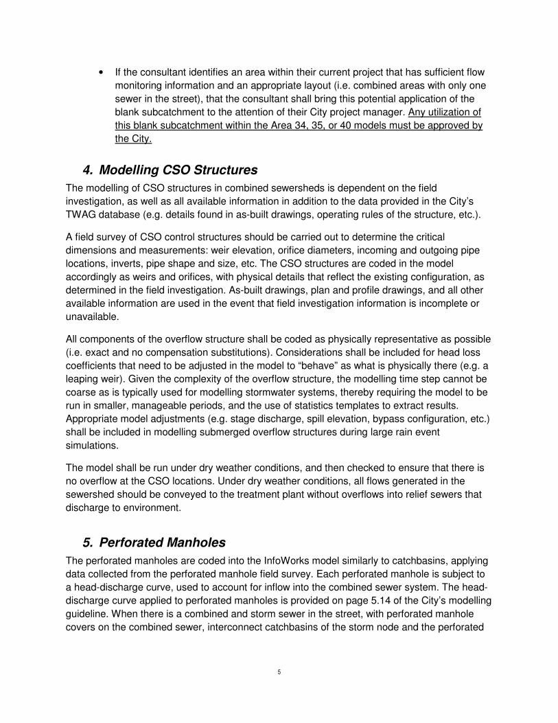
• If the consultant identifies an area within their current project that has sufficient flow
monitoring information and an appropriate layout (i.e. combined areas with only one
sewer in the street), that the consultant shall bring this potential application of the
blank subcatchment to the attention of their City project manager. Any utilization of
this blank subcatchment within the Area 34, 35, or 40 models must be approved by
the City.
4. Modelling CSO Structures
The modelling of CSO structures in combined sewersheds is dependent on the field
investigation, as well as all available information in addition to the data provided in the City’s
TWAG database (e.g. details found in as-built drawings, operating rules of the structure, etc.).
A field survey of CSO control structures should be carried out to determine the critical
dimensions and measurements: weir elevation, orifice diameters, incoming and outgoing pipe
locations, inverts, pipe shape and size, etc. The CSO structures are coded in the model
accordingly as weirs and orifices, with physical details that reflect the existing configuration, as
determined in the field investigation. As-built drawings, plan and profile drawings, and all other
available information are used in the event that field investigation information is incomplete or
unavailable.
All components of the overflow structure shall be coded as physically representative as possible
(i.e. exact and no compensation substitutions). Considerations shall be included for head loss
coefficients that need to be adjusted in the model to “behave” as what is physically there (e.g. a
leaping weir). Given the complexity of the overflow structure, the modelling time step cannot be
coarse as is typically used for modelling stormwater systems, thereby requiring the model to be
run in smaller, manageable periods, and the use of statistics templates to extract results.
Appropriate model adjustments (e.g. stage discharge, spill elevation, bypass configuration, etc.)
shall be included in modelling submerged overflow structures during large rain event
simulations.
The model shall be run under dry weather conditions, and then checked to ensure that there is
no overflow at the CSO locations. Under dry weather conditions, all flows generated in the
sewershed should be conveyed to the treatment plant without overflows into relief sewers that
discharge to environment.
5. Perforated Manholes
The perforated manholes are coded into the InfoWorks model similarly to catchbasins, applying
data collected from the perforated manhole field survey. Each perforated manhole is subject to
a head-discharge curve, used to account for inflow into the combined sewer system. The head-
discharge curve applied to perforated manholes is provided on page 5.14 of the City’s modelling
guideline. When there is a combined and storm sewer in the street, with perforated manhole
covers on the combined sewer, interconnect catchbasins of the storm node and the perforated

6
manhole of the combined node with an overland link, and assign a perforated head-discharge
curve to the combined node.
In areas with only a combined sewer, introduce a fictitious node beside the combined node
connected via a fictitious overland flow link and pipe link to the combined sewer system. Assign
a perforated head-discharge curve to the fictitious combined node to account for inflow.
6. Model Stability
When addressing model stability, applying Best Practices beginning in the model build stage is
important. The following practice is suggested to reduce model instability:
• Minimum pipe length: 5 m
• Do test runs using typical parameters (i.e. prior to calibration) to identify any points in
networks that are unstable or cause significant flooding or network water losses. The
cause of such instability may be caused by input outside the range of the model’s
realistic parameters, such as inappropriate loss coefficients, incorrectly sized junction
dimension, incorrect ponding areas or other default parameters in InfoWorks.
Modelers should always be on the lookout for signs of instabilities in the model. Instabilities
cause the following problems (from reference [1]):
If a model has instability problems, the procedure is to first do everything possible to resolve the
problem by making changes to the network. If the problem persists, the next step is adjusting
the Simulation Parameters default settings for the simulation’s maximum number of iterations
and the simulation’s maximum number of time step halving in InfoWorks. A step-by-step
approach should be taken. The time-step in the Schedule Hydraulic Run window should always
be set to 60 seconds. The first step is to run the model using the default conditions. If the model
does not converge, the next step is to increase the simulation’s maximum number of iterations;
this will allow the model to converge and stabilize. If increasing the number of iterations does

7
not help the model converge, increase the simulation’s maximum number of timestep halving.
According to [1], setting the tolerance for initialization and simulation volume balance to 0.005
will help model stability; this will eliminate volume imbalances above the threshold, but will
slightly slow down the simulation.
To summarize the approach to model stability:
1. Set the time-step (in the Schedule Hydraulic Run window) to 60s.
2. Run model using default settings
3. If the model does not converge, increase the simulation’s maximum number of iterations
4. If the model still does not converge, increase the simulation’s maximum number of
timestep halving
Notes:
The head-discharge curves associated with roof leaders for sloped and flat roofs are given in pages 5.25-26 in the
modelling guidelines.
The head-discharge curves for different types of catchbasins are given in pages 5.7-5.15.
Details of the set-up of fictitious node types in the model (either as a manhole or storage node) for roof areas are
given in page 6.8.
Reference [1]: Black & Veatch Wastewater Network Modelling Guide
Criteria for Provision of Level of Service
1. Flood protection criteria:
Any improvement works should not increase the WWF to the combined sewers for all
WWF conditions during the interim and ultimate stages. Opportunities for sewer
separation should be investigated.
The design criteria outlined in page 7.17 of the guideline will be followed in combined
sewer modelling. This section explains that the HGL shall be the same as the storm
system for the 100 year event. Annually, combined sewer overflows must meet the
objectives of MOE Procedure F-5-5 for volumetric control in a typical rainfall year from
April 1 to October 31 in continuous simulations. The typical rainfall year represents an
average rainfall year, not the 100-year design storm.
The storm system criteria in this section of the City’s modelling guideline states:
“…during the 100-year design storm, the maximum HGL in storm sewer (minor)
system shall be maintained at no surcharged conditions, while the overland flow
(major) system shall be maintained within the road allowance and no deeper
than the recommended standard as outlined in the Wet Weather Flow
Management Guidelines, City of Toronto, November 2006. Should it be infeasible
to achieve no surcharge conditions, the maximum HGL shall be maintained
below basement elevations during the 100-year design storm.”
The RFP however states the following in page 22 of 179:

8
“Design criteria shall be the City’s 100-year design storm. The maximum HGL in the
storm sewer (minor) system shall be maintained below basement elevations (1.8
m below the ground elevation) during the 100-year design storm. If it is not
feasible to maintain the maximum HGL at below basement, e.g. shallow storm
sewer system of which the crown of the sewer is less than 1.8 m below ground
elevation, the required level of protection shall be no surcharge condition.”
To summarize, the following approach will be taken (based on the RFP):
o Deep sewers:
� The maximum HGL shall be maintained below 1.8 m ground elevation(basement level)
o Shallow sewers:
� The no surcharge condition must be maintained
2. Water quality protection criteria:
Water quality criteria are to be addressed on two platforms: the MOECC’s F-5-5 and the
City of Toronto’s WWFMP. The F-5-5 applies specifically to CSOs, while the WWFMP
enforces water quality measures to reduce and eliminate adverse impacts of wet
weather flow to the built and natural environments and improve watershed health.
� MOECC F-5-5 Criteria
The guidelines of the MOECC’s Procedure F-5-5: determination of treatment
requirements for municipal and private combined and partially separated sewer
systems shall be followed. There will be no increases to volumes above the
existing levels in any CSO outfall structures, as outlined in the volumetric capture
criteria from the F-5-5 section 6.(g) in a typical rainfall year:
“During a seven-month period commencing within 15 days of April 1,
capture and treat for an average year all the dry weather flow plus 90% of
the volume resulting from wet weather flow that is above the dry weather
flow. The volumetric control criterion is applied to the flows collected by
the sewer system immediately above each overflow location unless it can
be shown through modelling and on-going monitoring that the criterion is
being achieved on a system-wide basis. No increases in CSO volumes
above existing levels at each outfall will be allowed except where the
increase is due to the elimination of upstream CSO outfalls. During the
remainder of the year, at least the same storage and treatment capacity
should be maintained for treating wet weather flow. ”
The RFP states the following in page 23 of 179:
“For study areas with combined sewer systems, treating combined sewer
overflows at CSO locations to achieve the Ministry of the Environment and
Climate Changes’ Procedure F-5-5 (i.e. during a seven-month period from
April to October in an average rainfall year, for 50% of the time, capture
and treat 90% of the wet weather flow that is above the dry weather flow,

9
to 30% BOD and 50% TSS reduction, whereas the TSS concentration should
not exceed 90 mg/L).”
This should be modified as follows to be consistent with the MOECC’s F-5-5 guidelines for combined sewer overflow structures:
During the 7 month period from April to October in an average rainfall year capture and treat 90% of the wet weather flow that is above the dry weather flow, to 30% BOD and 50% TSS reduction (primary treatment level). If the above volumetric criteria could not be achieved by sending the flow to the treatment plant, satellite treatment facilities should be provided. For the satellite treatment facilities the effluent TSS concentration should not exceed 90 mg/L for 50% of the time during the seven month period of the average year.
� City of Toronto WWFMP Criteria
As outlined in the RFP, water quality solutions must be consistent with the City of
Toronto’s 2003 WWFMP, addressing the voluntary and enhanced levels of wet
weather flow control (25- and 100-year implementation plans, respectively).
3. In order to successfully achieve the flooding and water quality criteria outlined in the
points listed above, the approach outlined in the following section can be followed.

10
Approach to Design Criteria
� Basement/Surface Flooding
1. Using the developed InfoWorks model for the 100-year design storm, establish the HGL and surcharge state in the combined and storm sewer systems under existing conditions.
2. Identify the potential problem areas and bottlenecks in the sewer system for the 100-year design storm. Propose basement and surface flooding control remediation measures to the combined and storm sewer systems to alleviate sewer surcharge, and to lower the HGL to a depth greater than 1.8 m below ground elevation (potential basement elevation). The overland flow depth must be maintained within the street right-of-way, i.e. 300 mm above road gutter elevation.
� MOECC F-5-5
3. Run the existing model to check the volume and frequency of overflows at the CSO structures under existing conditions for the typical year rainfall. The average year 1991-storm during the 7-month period from April to October should be applied to this simulation.
4. Repeat Step 3, using the model that includes the implementation of flood control remediation measures. Determine if there are any increases or decreases in the volume and/or frequency of spills for the typical year rainfall.
5. Provide and size control measures to mitigate increases in CSO spill volume and frequency if such is identified by the modelling of the ultimate condition (i.e. with implementation of flood control measures). There will be no increases in CSO overflow volumes following the implementation of basement and surface flooding remediation measures for the typical year rainfall.
� City of Toronto WWFMP
6. Use the average year 1991-storm to perform a continuous simulation during the 7-month period from April to October, generate a time series of flows (hydrographs) at the combined and storm sewer outfalls under existing conditions.
7. To be consistent with the 2003 WWFMP study, use the Event Mean Concentration (EMC) values of the four water quality parameters/pollutants for each land use: Total Phosphorus, Total Suspended Solids, Total Copper and E. coli from the WWFMP.
8. Using the EMC values from Step 7, calculate the pollutant concentration for the study area land use mix, and together with the flow hydrograph time series from Step 6, generate pollutographs to quantify the concentration and total loadings of the pollutants at the storm and combined outfalls under existing conditions.
9. Repeat Step 8, using the model that includes the implementation of flood control and CSO control remediation measures.

11
10. Implement various alternatives of source control, conveyance control, and end-of-pipecontrol measures, as stipulated in the 2003 WWFMP, to achieve water qualityimprovements at the storm outfalls and overflow from CSO structures. Establish (inSteps 11 and 12) two modelling scenarios to quantify for water quality improvements:
a. Voluntary level of wet weather flow control (25-year implementation plan) that willachieve moderate levels of enhancement to water quality parameters
b. Enhanced level of wet weather flow control (100-year implementation plan) thatwill achieve significant levels of enhancement to water quality parameters
11. Repeat Steps 6 and 8 for the Voluntary level of wet weather flow control using the modelthat includes the implementation of flood control and CSO control remediationmeasures.
12. Repeat Steps 6 and 8 for the Enhanced level of wet weather flow control using themodel that includes the implementation of flood control and CSO control remediationmeasures.
Summary
In summary, the approach requires:
• Proposing remediation measures to alleviate surface and basement flooding in the studyarea;
• Providing remediation measures to mitigate increases of existing CSO overflowfrequency and volumes from implementation of flood control measures; and
• Implementing the remedial measures identified in the WWFMP in a hierarchical form- with source controls considered first, followed by conveyance control measures then theend-of-pipe control measures.
Four separate model scenarios will result from the approach outlined in this section:
1. An existing model2. A model that includes remediation for basement/surface flooding and CSO control
measures3. A model that includes remediation for basement/surface flooding and CSO control
measures, as well as the voluntary level of water quality treatment4. A model that includes remediation for basement/surface flooding and CSO control
measures, as well as the enhanced level of water quality treatment

1
Dual Manhole Modelling Methodology (Excerpts from Current EA Study Areas 40 and 34)
EA STUDY AREA 40 DUAL MANHOLE MODEL SETUP Manhole structures identified to have a dual flow type are duplicated and connected to the appropriate system links to allow the network model to operate the local storm and sanitary system separately. The duplicated manhole structures were assigned a plan area of 0.8-0.9 m2, which is representative of the structure sizes observed though the Dual Manhole Investigation. Dual manhole cross-connections are simulated in the network model with a 1 m-long-250 mm diameter dummy pipe between the storm and sanitary manholes, the invert of this dummy pipe is set to the elevation of the identified cross-connection as discussed in the Modelling Methodology for Combined Sewer Areas Technical Memorandum. The links noted above also include dual MH cross-connections which act as a weir between the storm and sanitary systems. These were modelled as a flat dummy pipe with a diameter such that flow was not restricted as discussed in the Modelling Methodology for Combined Sewer Areas Technical Memorandum. DUAL MANHOLE RAMP-UP ASSESSMENT The dual manhole cross-connections were assessed to determine how often flows within the sanitary and storm systems would interact. It should be noted that the majority of the identified cross-connections within the inspected dual manhole were located at the most upstream ends of the sewer catchment areas, limiting the flow within the respective systems and the potential for system interactions. Table 6-8 identifies the design storm event at which time there is flow between the two systems. These dual manhole cross-connections have been included in the Area 40 model. The locations of these dual manhole cross-connections are shown in Figure 6-8 of Appendix A. Table 6-8: Dual Manhole Cross-Connection Ramp-Up Assessment
Dual Manhole ID Design Event With Flow in Cross-Connection
MH3886812404 50 year design storm
MH3876812001 Over 100 year
MH4001511905 Over 100 year
MH4016011454 50 year design storm
MH4022211172 100 year design storm
MH3844911415 Over 100 year
MH3975911448 Over 100 year
MH3933111270 25 year design storm
MH3957210889 Over 100 year
MH3967210860 Over 100 year

2
EA STUDY AREA 34 DUAL MANHOLE MODEL SETUP The available sewer database presents a total of two-hundred-and-sixty-three (263) manholes that were defined “dual” in Study Area 34. These manholes have sanitary and storm sewers in the same chamber divided by a wall that is intended to keep flows separated. An investigation was undertaken to confirm the hydraulic operation of each structure and to document possible cross-connections between the sanitary and storm sides of the structure. The results of this inspection show that twenty-one (21) dual manholes have conditions where flow could transfer between the storm and sanitary when surcharged. The locations of the DMO are shown in Figure A-10. The modelling time step and CSO and DMO structures has been carefully considered. A reduced time step to manageable periods, and the use of statistics templates to extract results. Appropriate model adjustments (e.g. stage discharge, spill elevation, bypass configuration, etc.) are included when modelling submerged overflow structures during large rain event simulations. Dual manholes were represented as a weir in the model. A dual manhole overflow occurs when the flow within the pipe reaches the weir crest and spills over from the sanitary to the storm sewer. Table 4-6: Dual Manhole Weir Parameters Used For Existing Condition Dual MH ID(1) Ground Elevation (m) Crest elevation (m) Width (m) Coefficient
Dual Manhole ID Ground Elevation (m)
Crest Elevation (m)
Width (m) Coefficient
MH4162122274 154.16 151.180 1.35 0.57
MH4136022355 148.163 144.593 1.35 0.57
MH4128222378 144.499 142.604 1.35 0.57
MH4225323018 158.502 155.872 1.04 0.57
MH4263323202 155.434 152.734 1.67 0.57
MH4086223492 155.71 153.473 1.82 0.57
MH4093223470 156.064 153.249 1.35 0.57
MH4095723562 155.887 153.666 1.36 0.57
MH3948510915 Over 100 year
MH4206110609 50 year design storm
MH4201010440 Over 100 year
MH4002110929 Over 100 year
MH4005810799 Over 100 year
MH4006010654 Over 100 year
MH3985310619 10 year design storm
MH3985010597 50 year design storm
MH4010310250 50 year design storm
MH3989610099 50 year design storm
MH3970210101 2 year design storm
MH3884111304 25 year design storm

3
MH4100223447 155.765 152.903 1.35 0.57
MH4102823539 154.525 152.030 1.35 0.57
MH4175724162 159.182 156.427 1.38 0.57
MH4189424227 160.000 157.528 1.36 0.57
MH4260924206 156.307 152.477 1.15 0.57
MH4261123974 155.131 152.254 1.37 0.57
MH4269123949 155.084 153.114 1.36 0.57
MH4271524666 165.266 162.421 1.36 0.57
MH4289524729 169.045 165.725 1.8 0.57
MH4298224758 169.740 166.495 1.37 0.57
MH4299823751 159.467 156.747 1.16 0.57
MH4306323969 161.721 159.261 1.16 0.57
MH4317024418 167.572 165.072 1.11 0.57
DUAL MANHOLE RAMP-UP ASSESSMENT The DMO assessment results indicate that during events smaller than the 5-year design storm, no DMOs are predicted to occur. However, during the May 12, 2000 event and the May 28, 2012; one (1) dual manhole was predicted to overflow. The location of this DMO structure is on Marta Avenue, where the HGL in the sanitary sewer system is within basement levels. Table 7-2: Predicted Dual Manhole Overflows

Project Name: Basement Flooding Remediation, Area 40 Project Code: WSP15-0004 Task: Dual Manhole Investigation Location: 110 Forest Hill Road Date and Time: May 20th, 2016 at 1:10PM
Manhole ID: MH 34, MH3886812404
Sewer Lines
Chamber
Weirs/Orifices
Notes/Drawings
Plan
- Sanitary sewer has an inlet diameter of 0.25m, outlet diameter of 0.30m and a flow of 0.02m deep - Storm sewer has an inlet diameter of 0.30m, outlet diameter of 0.36m and no flow, contains debris
- Total manhole depth is 4.24m - Made of brick
- Has a weir separating the sewer lines that is 1.20m in length, 0.10m wide and 2.10m tall on the sanitary sewer side and 1.55m tall on the storm sewer side.
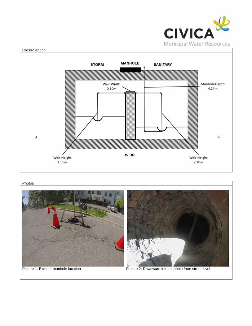
Cross-Section
Photos
Picture 1: Exterior manhole location Picture 2: Downward into manhole from street level
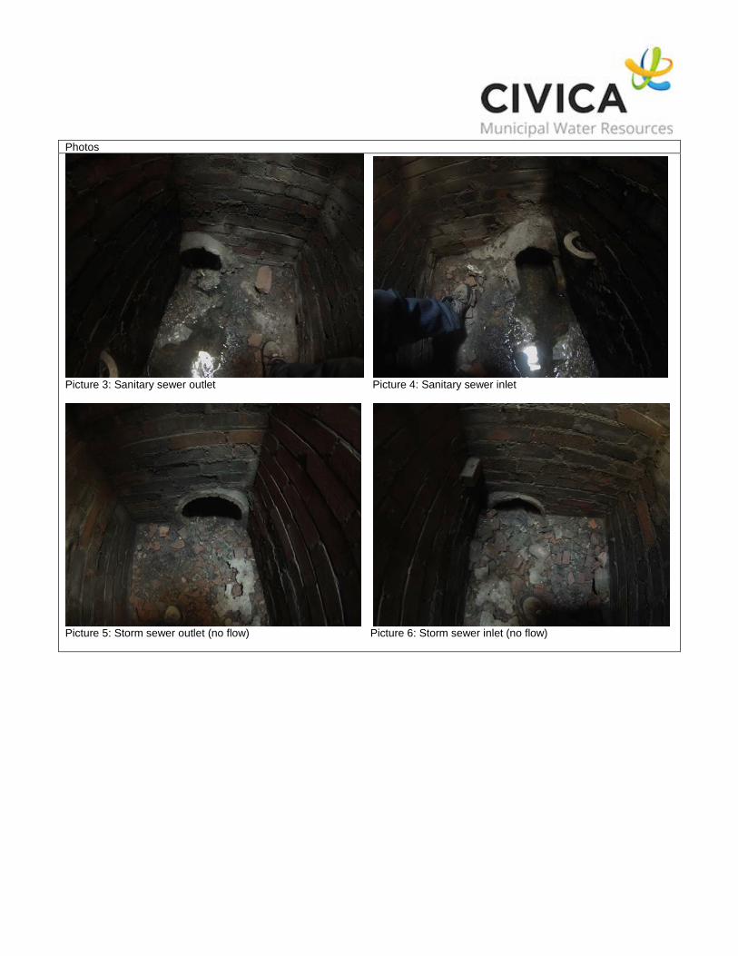
Photos
Picture 3: Sanitary sewer outlet Picture 4: Sanitary sewer inlet
Picture 5: Storm sewer outlet (no flow) Picture 6: Storm sewer inlet (no flow)

Engineering and Construction Services Draft Perforated Modeling Spec - Basement Flood Area 34 April 14, 2016
Page ii
Table of Contents
1.0 Perforated Manholes ..................................................................................................... 1
1.1.Street with One Sewer – Combined Sewer Only. ............................................................. 1 1.1.1. Combined Perforated Manhole ....................................................................................... 1
1.2.Street with Two Sewers (Sewer Separation) – Combined/Sanitary (Partial) and Storm Sewer. ....................................................................................................................................... 1 1.2.1. Combined/Sanitary Perforated Manhole ......................................................................... 1 1.2.2. Storm Perforated Manhole .............................................................................................. 1
1.3.Street with Three Sewers (Sewer Separation) – Combined (Partial), Sanitary, and Storm Sewer. ............................................................................................................................ 1 1.3.1. Combined Perforated Manhole ....................................................................................... 1 1.3.2. Sanitary Perforated Manhole .......................................................................................... 1 1.3.3. Storm Perforated Manhole .............................................................................................. 1
1.4.Naming Convention ........................................................................................................... 1

Engineering and Construction Services Draft Perforated Modeling Spec - Basement Flood Area 34 April 14, 2016
Page 1
1.0 PERFORATED MANHOLES
The perforated manholes are coded into the InfoWorks model similarly to catchbasins, applying data collected from the perforated manhole field survey. Each perforated manhole is subject to a head-discharge curve, used as a hydraulic control to dictate how much water from the overland system is captured into the sewer system. The section below describes how a head-discharge curve should be applied for the possible sewer configurations.
1.1. Street with One Sewer – Combined Sewer Only.
1.1.1. Combined Perforated Manhole
Introduce a fictitious combined node beside the combined node to assign a perforated head-discharge curve to the fictitious combined node to account for the flow entering through the perforated manhole.
Interconnect catchbasins of the combined node and the fictitious combined node with an overland link, and assign the catchbasin head-discharge curve to the combined node.
1.2. Street with Two Sewers (Sewer Separation) – Combined/Sanitary (Partial) and Storm Sewer.
1.2.1. Combined/Sanitary Perforated Manhole
A perforated head-discharge curve is assigned to the combined/sanitary node.
1.2.2. Storm Perforated Manhole
Introduce a fictitious node beside the storm node to assign a perforated head-discharge curve to the fictitious storm node to account for the flow entering through the perforated manhole.
Interconnect catchbasins of the storm node and the fictitious storm node with an overland link, and assign the catchbasin head-discharge curve to the storm node.
Interconnect catchbasins of the storm node and the perforated combined/sanitary manhole with an overland link.
1.3. Street with Three Sewers (Sewer Separation) – Combined (Partial), Sanitary, and Storm Sewer.
1.3.1. Combined Perforated Manhole
A perforated head-discharge curve is assigned to the combined node.
1.3.2. Sanitary Perforated Manhole
A perforated head-discharge curve is assigned to the sanitary node. To be modelled only during calibration and assessment of existing conditions. However, during remediation, all perforated manhole covers should be replaced with 2 pick holes or solid covers.
1.3.3. Storm Perforated Manhole
Introduce a fictitious node beside the storm node to assign a perforated head-discharge curve to the fictitious storm node to account for the flow entering through the perforated manhole.
Interconnect catchbasins of the storm node and the fictitious storm node with an overland link, and assign the catchbasin head-discharge curve to the storm node.
Interconnect catchbasins of the storm node and the perforated combined/sanitary manhole with an overland link.
1.4. Naming Convention
The naming convention of fictitious ‘Dummy” nodes shall follow section 4.5.1.3 of the City’s Modeling Guidelines.

M32445301002_FINAL 1 04/13/16
Date: April, 13, 2016 XCG File No.: 3-244-53-01
To: Andrea Ramsey, Vicky Shi, Allen Li, City of Toronto
From: Philip Gray, XCG Consultants Ltd.
Re: Approaches to Modelling Ditch Drainage - Discussion Paper
1. INTRODUCTION The following discussion paper considers different methodologies to modelling road side ditch drainage systems within the InfoWorks modelling framework. The ideas put forward are for discussion and assume the reader understands the modelling capabilities of InfoWorks.
To model roadside drainage ditches the following was considered:
• Extent and variety of ditch drainage systems (residential, ICI areas, along larger collector roads, etc.).
• The transition from ditch to curb-gutter cross sections.
• Interaction between ditch drainage and storm conduits. Some areas have storm conduits as well as ditch drainage, other streets have ditch drainage only.
• Variability in ditch cross sections.
• Representing the ditches as RIVER or OVERLAND CONDUIT systems; Flow Types as STORM, OVERLAND or OTHER
• Recognition of different roughness, losses through driveway culverts or other impediments.
• Thematic mapping of results and criteria for overland flow depth.
In Basement Flooding Area 36 (Area 36), there are some municipal roadway segments with ditch drainage systems. Some of these roadway segments are located within the ICI area upstream of Highway 401, and some are located in the residential area south of Dixon Road and west of Royal York Road. Locations are documented in Area 36 Technical Memorandum #1.
Figure 1 and 2 show sample "street view" photographs that typify the type of ditches in Area 36 (from Google Earth, February 2016). The photographs show the differences in ditch cross section with Figure 1 showing a more defined ditch on the left side and little or no ditch on the right side. Figure 2 shows a more uniform cross section for both sides of the road.
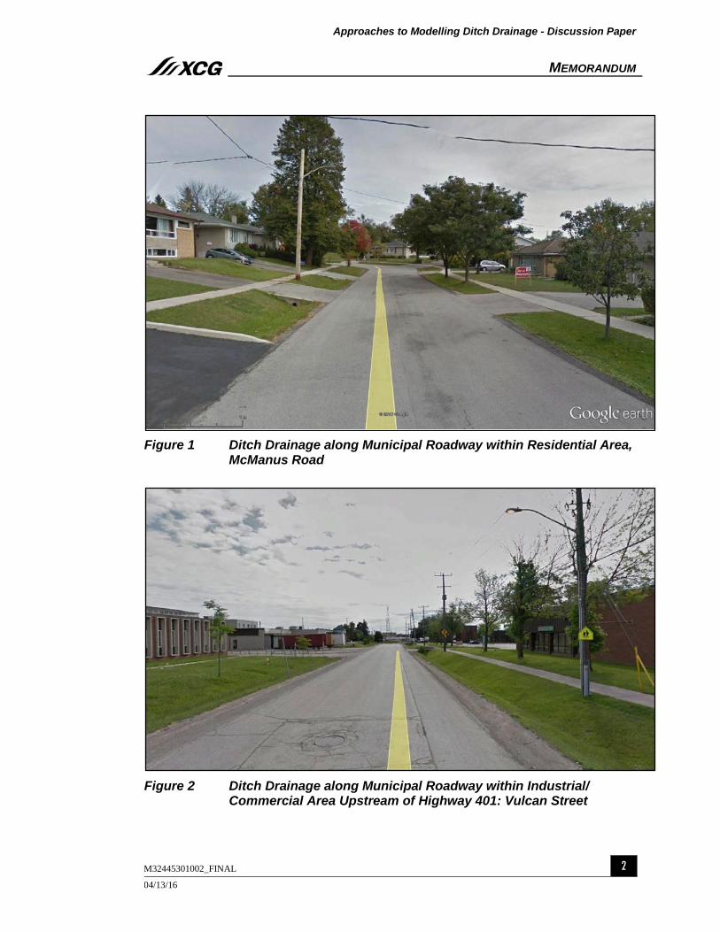
Approaches to Modelling Ditch Drainage - Discussion Paper
MEMORANDUM
M32445301002_FINAL 2 04/13/16
Figure 1 Ditch Drainage along Municipal Roadway within Residential Area, McManus Road
Figure 2 Ditch Drainage along Municipal Roadway within Industrial/ Commercial Area Upstream of Highway 401: Vulcan Street
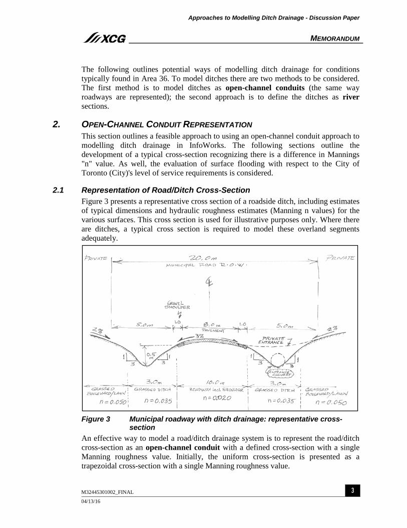
Approaches to Modelling Ditch Drainage - Discussion Paper
MEMORANDUM
M32445301002_FINAL 3 04/13/16
The following outlines potential ways of modelling ditch drainage for conditions typically found in Area 36. To model ditches there are two methods to be considered. The first method is to model ditches as open-channel conduits (the same way roadways are represented); the second approach is to define the ditches as river sections.
2. OPEN-CHANNEL CONDUIT REPRESENTATION This section outlines a feasible approach to using an open-channel conduit approach to modelling ditch drainage in InfoWorks. The following sections outline the development of a typical cross-section recognizing there is a difference in Mannings "n" value. As well, the evaluation of surface flooding with respect to the City of Toronto (City)'s level of service requirements is considered.
2.1 Representation of Road/Ditch Cross-Section Figure 3 presents a representative cross section of a roadside ditch, including estimates of typical dimensions and hydraulic roughness estimates (Manning n values) for the various surfaces. This cross section is used for illustrative purposes only. Where there are ditches, a typical cross section is required to model these overland segments adequately.
Figure 3 Municipal roadway with ditch drainage: representative cross- section An effective way to model a road/ditch drainage system is to represent the road/ditch cross-section as an open-channel conduit with a defined cross-section with a single Manning roughness value. Initially, the uniform cross-section is presented as a trapezoidal cross-section with a single Manning roughness value.

Approaches to Modelling Ditch Drainage - Discussion Paper
MEMORANDUM
M32445301002_FINAL 4 04/13/16
Figure 4 shows an example comparison of rating curves for the actual road/ditch section and a trapezoidal approximation, for the specific case noted in Figure 3. The rating curve for the actual section has been computed by calculating a separate conveyance term for each cross-section segment with different Manning n value, this being the same approach used, for example, in the HEC-RAS model to account for differences in hydraulic roughness across a river cross-section. For the trapezoidal section approximation, a single Manning n value is applied across the entire section.
Figure 4 Rating Curve for Roadway Ditch System, and Trapezoidal Approximation This approximation closely matches the depth-flow relationship for depths below the top of the roadway. Above the top of the road surface, the trapezoidal approximation underestimates flow for a given depth. This would effectively mean that the hydraulic analysis under extreme conditions (i.e. roadway surface entirely flooded) is conservative in the sense that the depth of flooding would be somewhat overestimated.
At this stage it is unknown if such extreme conditions would be computed by the model during events as large as the 100-year event. Model results would require careful review in this respect to ensure the use of a trapezoidal section approximation is not resulting in overestimation of surface flooding.
In representing a road/ditch section in this manner, the City level of service with respect to "depth of surface flooding" will be different than the typical road cross-section. The metric of overland flow depth being less than 300 mm is not directly

Approaches to Modelling Ditch Drainage - Discussion Paper
MEMORANDUM
M32445301002_FINAL 5 04/13/16
applicable to the trapezoidal section. For each road-ditch section a unique overland flow depth (depth of flow) will need to be established to define acceptable performance.
In the context of InfoWorks and thematic mapping showing performance, this representation is problematic. For roadways one thematic group can be used, in this case a unique depth will need to be determined that defines a problem level associated with each ditch system. Great care would be required to ensure the correct performance measure (depth of flow) is applied to the right overland flow section.
2.2 Thematic Mapping - Open Channel Conduit To address the issue of thematic mapping and to make the process of review more uniform the initial trapezoidal representation is taken one step further. Instead of using a trapezoid shape, it is also possible to represent the road/ditch section as a flat- bottomed channel such that one thematic group definition would apply to all overland conduit sections.
For the open-channel conduit to be equivalent in regards to flow capacity, the total carrying capacity of the road/ditch section must equal the total carrying capacity of the open-channel conduit. Not including the conduit roughness, there are two parameters that can be adjusted to change the open-channel conduit carrying capacity; width and depth. To use a single theme group to display the results of the overland flow system a maximum depth of 300 mm was set for the open-channel. Once the 300 mm depth is reached, the road/ditch section would be at capacity. In other words, if the flow in the open-channel conduit exceeded the peak carrying capacity and spilled onto private property, the flow depth in the open-channel conduit would be greater than 300 mm. This corresponds then with the curb and gutter road level of service overland flow depth not exceeding 300 mm.
Following a similar process used initially for the trapezoid representation, an equivalent flat-bottomed open channel can be developed that has the same carrying capacity of the road/ditch system. In this case, the width of the flat bottom channel is calculated such that the critical depth of flow in the road/ditch section is equivalent to a depth of flow of 300 mm in the flat-bottom channel. Figure 5 shows an equivalent flat-bottom open-channel conduit for a typical ditch/road section.
Figure 5 Flat-Bottom Representation
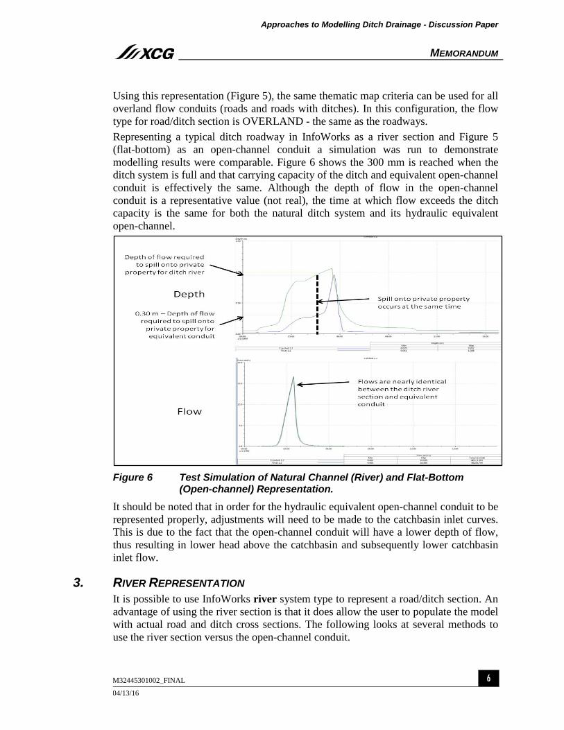
Approaches to Modelling Ditch Drainage - Discussion Paper
MEMORANDUM
M32445301002_FINAL 6 04/13/16
Using this representation (Figure 5), the same thematic map criteria can be used for all overland flow conduits (roads and roads with ditches). In this configuration, the flow type for road/ditch section is OVERLAND - the same as the roadways.
Representing a typical ditch roadway in InfoWorks as a river section and Figure 5 (flat-bottom) as an open-channel conduit a simulation was run to demonstrate modelling results were comparable. Figure 6 shows the 300 mm is reached when the ditch system is full and that carrying capacity of the ditch and equivalent open-channel conduit is effectively the same. Although the depth of flow in the open-channel conduit is a representative value (not real), the time at which flow exceeds the ditch capacity is the same for both the natural ditch system and its hydraulic equivalent open-channel.
Figure 6 Test Simulation of Natural Channel (River) and Flat-Bottom (Open-channel) Representation. It should be noted that in order for the hydraulic equivalent open-channel conduit to be represented properly, adjustments will need to be made to the catchbasin inlet curves. This is due to the fact that the open-channel conduit will have a lower depth of flow, thus resulting in lower head above the catchbasin and subsequently lower catchbasin inlet flow.
3. RIVER REPRESENTATION It is possible to use InfoWorks river system type to represent a road/ditch section. An advantage of using the river section is that it does allow the user to populate the model with actual road and ditch cross sections. The following looks at several methods to use the river section versus the open-channel conduit.

Approaches to Modelling Ditch Drainage - Discussion Paper
MEMORANDUM
M32445301002_FINAL 7 04/13/16
3.1 RIVER Approach 1 This initial river configuration has the following features:
• The road/ditch section has a storm sewer as well.
• The river section is connected to the storm system with inlets.
• River cross section is defined where the crown of the road is the rim elevation of the maintenance hole. The elevation of the cross-section is relative to the rim elevation such that the ditch elevations are below the rim elevation.
• The flood elevation is the rim elevation (a lower flood elevation was also tried).
• River section is defined with OVERLAND flow type.
Figure 7 shows the general InfoWorks set up, cross-section profile and long-section.
Figure 7 RIVER Approach 1 Setup Since the river section is part of the major flow system, it was given a system type of OVERLAND. However, InfoWorks CS, after version 12, does not permit OVERLAND type rivers or conduits to have inverts below the specified ground elevation at its upstream and downstream manholes. Figure 8 shows the error message. Consequently, this approach is not valid.

Approaches to Modelling Ditch Drainage - Discussion Paper
MEMORANDUM
M32445301002_FINAL 8 04/13/16
Figure 8 InfoWorks Error Message - RIVER Approach 1
3.2 RIVER Approach 2 Building on the previous approach, the river section flow type was changed from OVERLAND to STORM. InfoWorks does allow a river section with a STORM system type to have inverts below the ground elevation.
Although this configuration allows inverts below the ground elevation, this configuration does not function correctly. Because the flow type is STORM, runoff from a catchment will first go through the INLET structure before flow enters either the storm conduit or the river section. When the inlet capacity is exceeded it is expected the excess flow would enter the river section, but this does not happen. Because the river section is defined as STORM, flow in excess of the inlet capacity is stored at the inlet until it can enter the storm system, which includes the river sections and storm conduits. The INLET effectively regulates the flow into both the storm conduit and the river section.
Figure 9 shows the results of this test condition. Flow at the upstream node ponds until it can enter the storm system, no flow was registered in the river section. It is expected if the storm conduit surcharges to the invert of the river section flow would appear in the river section. But flow in excess of the inlet capacity does not enter the river section with the STORM flow type. Only if the river section is OVERLAND would flow in excess of the inlet capacity enter the river section, but the Approach 1 error would occur.

Approaches to Modelling Ditch Drainage - Discussion Paper
MEMORANDUM
M32445301002_FINAL 9 04/13/16
Figure 9 RIVER as STORM Flow Type - River Approach 2 (NEED TO REVIEW)
3.3 River Approach 3 A third configuration, presented in Figure 10, involves offsetting the river section from the storm sewer and connecting it via a catchbasin lead (or equivalent).
For this model set up, the ground elevation of the overland (river) nodes used to connect the river section to the storm conduit would be the maintenance hole rim elevation, less the depth to the lowest part of the ditch. This river node elevation represents the elevation of a catchbasin inlet in a ditch. The connecting conduit from the river node to the storm node acts effectively like a catchbasin lead. The size of that lead becomes important because it could act as a restriction under some conditions.
This approach works, but there are several things to consider:
• The size of connecting conduits is important so they do not cause restrictions. This is important if additional inlet capacity is recommended; if the connection size is not increase, then the simulation results may not be reasonable.
• The thematic group to illustrate results will be different for each ditch section.

Approaches to Modelling Ditch Drainage - Discussion Paper
MEMORANDUM
M32445301002_FINAL 10 04/13/16
Figure 10 RIVER Approach 3 Setup
3.4 River Approach 4 Building on the previous discussion, it is possible to use the river section and have the storm node rim elevations as the invert of the ditch. In this situation, the river section can be defined as overland and it will not have Approach 1 problems.
The issue with this approach includes:
• The rim elevations may not reflect the slope of the ditch.
• A unique theme group will be needed to show performance.
• Transition from and to road sections need to be managed.
4. SUMMARY The following is concluded:
• Using an equivalent open-channel conduit to represent a road/ditch system is a suitable approach and can be configured such that the thematic group for maximum surface flow depth can be used.
• A representative Mannings "n" can be determined to represent the different roughness in the road/ditch cross section.
• Using the river section is possible, but requires careful consideration with respect to the how it is configured with the pipe network, defining elevations, and transitions to roadway sections.

Approaches to Modelling Ditch Drainage - Discussion Paper
MEMORANDUM
M32445301002_FINAL 11 04/13/16
Other factors to consider:
• Consideration needs to be given to the transition from road/ditch system to a typical curb and gutter road section. Ditches tend to end at inlets that are below the road surface. Only when the ditch fills up will overland flow enter the downstream overland system. Connecting links (transitions) will need to be added to connect road/ditch model elements the road cross section.
• Catchbasin inlet curves for open-channel conduits would need to be modified to correspond with the ditch inlet curves recognizing the head on a ditch inlet and in the open-channel inlet would be different for the same inlet capacity.
5. OTHER FACTOR
5.1 Level of Service - Ditches The City has a well-established approach to defining the level of service for overland flow on roadways as documented in the model guidance document. The level of service is based on the maximum depth of flow being less than 300 mm. At this maximum depth, it is assumed that the surface water will not leave the municipal right of way.
With ditches, the cross section is not always well defined. Therefore, the maximum depth of flow can be greater than 300 mm in the ditch before it impacts the road or may extend beyond the right of way. Each ditch segment will be different, and it may vary along a ditch system.
The City should consider establishing a level of service criteria for ditches. The following criterion is suggested:
• The maximum depth of flow in a ditch should not exceed the elevation of the pavement edge less the ditch invert.
This level of service criterion assumes the pavement edge is at a similar elevation as the right of way (property line). It is also based on a general safety concern that if the ditches are full, and water extends across a roadway, a driver would not have a sense of the water depth at the edge of the road. With a curb and gutter cross section the depth of water is relatively clear, not with a ditch.
This criterion is suggested only and has no standing with Toronto Water.
5.2 Wide Roads In Area 36 there are no ditch drainage systems adjacent to wide collector roads. However, the following comments are made:
• For wide roads it may be better to represent the ditches as two separate parallel overland systems.
• It is feasible the overland contribution from one side of the road could be quite different from the other side. Also on wide roads it is not uncommon to have two storm systems.
• If needed, a connection between the parallel overland systems can be added.
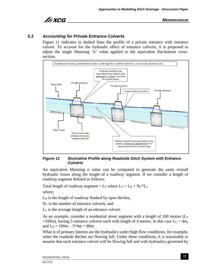
Approaches to Modelling Ditch Drainage - Discussion Paper
MEMORANDUM
M32445301002_FINAL 12 04/13/16
5.3 Accounting for Private Entrance Culverts Figure 11 indicates in dashed lines the profile of a private entrance with entrance culvert. To account for the hydraulic effect of entrance culverts, it is proposed to adjust the single Manning "n" value applied to the equivalent flat-bottom cross-section.
Figure 11 Illustrative Profile along Roadside Ditch System with Entrance Culverts
An equivalent Manning n value can be computed to generate the same overall hydraulic losses along the length of a roadway segment. If we consider a length of roadway segment defined as follows:
Total length of roadway segment = LT where LT = LD + NC*LC
where;
LD is the length of roadway flanked by open ditches,
NC is the number of entrance culverts, and
LC is the average length of an entrance culvert.
As an example, consider a residential street segment with a length of 100 metres (LT =100m), having 5 entrance culverts each with length of 4 meters. In this case LC = 4m, and LD = 100m – 5*4m = 80m.
What is of primary interest are the hydraulics under high flow conditions; for example, when the roadside ditches are flowing full. Under these conditions, it is reasonable to assume that each entrance culvert will be flowing full and with hydraulics governed by

Approaches to Modelling Ditch Drainage - Discussion Paper
MEMORANDUM
M32445301002_FINAL 13 04/13/16
"outlet control" conditions (as opposed to "inlet control"). Refer to Figure 11. Over any road segment, the total hydraulic losses can be computed as
Total hydraulic losses = HD + NC*HC
Where HD are hydraulic losses along the open ditch segments, and
HC is the average hydraulic loss at an individual entrance culvert.
The losses along the open ditch segments can be computed using the equivalent flat-bottom section. The losses can be computed (from Manning equation) as;
HD = LD*VD2 * nD
2 / RD1.3333
where
VD is the flow velocity in the open ditch,
nD is the Manning n value for the open ditch, and
RD is the hydraulic radius in the open ditch (area / wetted perimeter).
Losses at each entrance culvert will be the summation of entrance losses (typically calculated using an entrance loss coefficient applied to pipe velocity head) and pipe friction losses.
To generalize the analysis, assume private entrance culverts are corrugated steel pipe culverts (n=0.024) with typical diameter of 500 mm, typical length of 4 metres and a hydraulic entrance loss coefficient of 0.70.
Using these assumptions, under full ditch conditions with depth of flow on the upstream side of the entrance culvert of approximately 0.60 metres, flow through the culvert will be approximately 0.35 m3/s with hydraulic losses of approximately 0.24 metres.
Using the above equations, an equivalent Mannings n value for the representative ditch section can be computed to account for culvert losses, as follows:
nE = √ [ (LD*VD2*nD2/RD
1.3333 +NC*HC)*RD1.333 / (LT * VD
2)]
Where nE is the equivalent Manning n value to account for the compound losses.
Example: Using the trapezoidal cross-section described in Figure 4, (Bottom width 0.0 m, sideslopes 8:1 H:V, n=0.030, long slope = 0.003 m/m), at full ditch conditions for a total roadway segment length (LT) of 100 metres with 5 entrance culverts of average length (LC) of 4 metres (and therefore LD = 80 m):
VD = 0.6 m/s
RD = 0.17 m
and using HC = 0.24 m
then nE = 0.067
This value is an increase in the Manning n value applied to the open ditch of 0.037 (i.e. increase from 0.030 to 0.067). This pertains under high flow conditions. This outcome reflects the fact that under high-flow conditions, the losses at entrance culverts (NC*HC) become a dominant consideration.

Approaches to Modelling Ditch Drainage - Discussion Paper
MEMORANDUM
M32445301002_FINAL 14 04/13/16
6. RECOMMENDATIONS The following recommendations are made:
• Typical ditch cross sections are required where there are ditches.
• Where there are storm pipes and maintenance holes associated with the ditch system, cross sections at each maintenance hole should be collected and associated with the maintenance hole rim elevation. Other cross sections may be required.
• Represent the ditch systems as flat-bottom open-channel conduits. The conduit width would be adjusted so the maximum conveyance capacity of the ditch is reached when the open-channel representation is 300 mm in depth.
• A single Manning roughness value will be determined for each cross section based on the roughness of the roadway and ditch characteristics.
• Transition sections are required between ditch and curb/gutter overland systems.
• Develop equivalent catchbasin inlet curves where the ditch systems are represented as flat-bottom open-channel conduits.
Using an equivalent flat-bottom cross section is consistent with how roadways are modelled as overland flow channels. It is possible to have a different equivalent cross-section shape if required.
Ideas to be discussed further include:
• Establishing a level of service criterion for ditches (i.e. the maximum depth in a ditch will not be higher than the pavement edge).
• Should additional losses be associated with driveway culverts in the representation of ditches?

Evaluation of Climate Change The effects of climate change on the preferred solutions proposed in this EA study will be evaluated by the Consultant. A sensitivity analysis will be conducted by the Consultant to determine the impact of climate change on the size of the sewer upgrades and storage volumes proposed (e.g. determine the percent increase in the size of the sewer upgrade or storage volume due to increase in the rainfall volume and intensity) and conduct a risk assessment of the preferred solutions for the 100-year design storm for the storm system and the May 12, 2000 storm for the sanitary system (equivalent to a 25 to 50-year storm) to identify those preferred solutions that can result in significant damages and losses if failure were to occur. Such preferred solutions need to have higher operation and maintenance priorities and frequencies. Sewer systems are comprised of assets with long design lives. Current climate change predictions indicate that severe weather events will become more frequent in the future. The rainfall volume, intensity, storm duration and the interval between storms are changing. More intense, extreme rainstorms are expected, especially during summer periods. Rainfall increases lead to increases in surface runoff and flood volumes. The effects are expected to combine with relative increase in impermeable surfaces due to urbanization, and to a certain extent changing antecedent rainfall conditions that can further increase the percentage of runoff. As rainfall intensity changes, a 1 in 100 year storm could become an event with a 1 in 75 year return period. Flood protection designs need to be capable of accepting increased flows to avoid flooding at more frequent intervals, for example, designing the major system with a safety factor to take more flows and diverting the excess flow by flood relief pathways. Climate change studies have reported that rainfall volumes and intensities could increase by 20% by 2085 and that the dry weather period between storms could increase up to 100%, especially in summer. The multipliers listed in the table below have been applied in urban drainage calculations.
Table - Climate Change Factors
Return Period 2 Year 10 Year 100 Year Climate Factor 1.2 1.3 1.4
A risk analysis of the system can be undertaken to examine how the drainage systems would perform under different extreme rain events and to prioritize the maintenance and operational actions that should be undertaken to minimize flooding risks. The focus should be on those parts of the drainage system, where failure due to climate change can result in significant flood damages and property losses upstream or downstream. The ultimate goal is to ensure that the effectiveness of the proposed basement flooding solutions for their anticipated design life. The consultant is encouraged to propose a refined methodology for achieving this goal in a comprehensive and cost effective manner.

Consideration of Blockage in Sewer and Sewer Condition Model setup assumes that the sewers are clean and the roughness coefficients are the same as of the new sewers. In practice, old storm sewers can be blocked with sediments and debris while old sanitary sewers may be blocked with sediments, calcite, or grease deposits. Control measures will not work well if blockages are present downstream. The best approach for determining actual sewer conditions and possible blockages in sewers is to review CCTV records to confirm the condition of the sewers. With this check, an alert can be included in the specifications during design and construction of the basement flooding control works to clean the sewers, or extend the improvements to include rehabilitating or replacing the blocked sewers. The adjustments can be covered under ‘state of good repair’ capital budget. Since CCTV may not be available for all the pipes, the following checks and sensitivity analyses are to be conducted to identify potential blockages downstream of the proposed control measures locations: a) Identify frequent flushing locations – obtain and review sewer flushing records from District
Operations. These sewer sections may have blockages. b) Age of Sewers – old storm and sanitary sewers are more likely blocked with sediments, debris, calcite,
and grease deposits. A GIS plot can be made to show sewer age and identify their locations where proposed basement flooding control measures may be affected. Sensitivity analyses of Manning’s roughness can be carried out for these sewers by increasing the Manning’s roughness based on the age of the sewers, such as:
Sewer Age Manning’s Roughness Coefficient For Concrete Pipes
0 to 9 years 0.013 10 to 19 years 0.015 20 to 29 years 0.017
30 years and greater 0.019 c) Low or negative pipe slope – storm and sanitary sewers with low or negative pipe slope are more
likely to have sediments, debris, calcite, and grease deposits. A plot with GIS can be made to show sewers with pipe slope less than 0.1% and identify their locations where proposed basement flooding control measures may be affected.
d) Low flow velocity - For sanitary sewers, low peak DWF velocity (less than 0.6 m/s) could be a good
indicator for a pipe which may likely to have problems with sediments, debris, calcite, and grease deposits; review flow monitoring data and modelled flow velocity
Checking the sewers downstream of proposed control measures can therefore include the following steps: a) Review CCTV records of the existing sewers at and downstream of the recommended basement
flooding solution; if required, include cleaning, rehabilitation, and replacement of the clogged sewers in the recommended alternative to be carried out during design and construction,

b) Overlay the frequent flushing locations, age of sewers, pipe slope, and sewer flow velocity by GIS mapping, sewers with overlapping data can be potential ‘hot spots’, and
c) Provide additional allowance in the design if the recommended basement flooding control measure
is located upstream of these ‘hot spots’. The ultimate goal of this provisional task is to ensure that the effectiveness of the proposed basement flooding solutions is not impeded by deficient downstream sewers. The consultant is encouraged to propose a refined methodology for achieving this goal in a comprehensive and cost effective manner as part of the proposal.

For Consultants
EA Study TM#4 - Area XX- Checklist Date Reviewed By QA/QC Staff Date Reviewed By Project Manager
RFP No. :
TM# 4 Revision:
Consultant: MM/DD/YYYY
IW Model Version:
Section Description of Check Yes
No
(in
clu
de
det
ails
in c
om
men
ts)
Fully
Co
mp
lian
t
Co
mp
lian
t w
ith
res
erva
tio
ns
(in
clu
de
det
ails
in c
om
men
ts)
No
n C
om
plia
nt
(in
clu
de
det
ails
in c
om
men
ts)
1 Model Build, Calibration and Validation (incl. conformance to Modelling Guidelines - modelling guideline sections referenced below)
1.0 Does the model reflect data provided
a GIS Data
b Field investigations
c As-built drawings (note where as-built checked)
d Other (please list)
1.1 File Management, Naming and Data Flagging (Section 4)
a Catchment group hierarchy set-up (Section 4.2)
b Documentation of noteworthy details in Description Field (Section 4.3)
c Model Groups set-up (Section 4.4)
d Naming Convention (Section 4.5)
e Data Flagging (Section 4.6)
f Simulation Parameters, including Volume Balance = 0.01 (Section 4.7)
g Default Time Step (Section 4.7.1)
h Element documentation (Section 4.8)
i Model visualization (Section 4.9)
j All other Section 4 requirements
1.2 Major System Continuity (Section 5.1.2)
1.3 Node Set-up, including the appropriate Head-Discharge Tables (Section 5.2)
aThe assignment of catchbasins to nodes was verified to ensure that the # of CBs assigned to a node reflects the
actual number of catchbasins that collect overland flow and contribute flow to the appropriate sewer/link?
1.4 Sewer links set-up (Section 5.3)
a Continuous system connectivity (i.e. upstream trace)
b No pipes with negative gradient
cNo node backdrop in the system (i.e. the invert of incoming pipe at a MH is less than invert of outgoing pipe at
the same MH)
dManning's roughness coefficients for sewers and overland flow paths are set based on guidelines (Appendix B.2
of the Modelling Guidelines)
1.5 Overland Connectivity Set-up (Section 5.4)
a Overland link flag set to #D (Default)
b Verify overland flow connectivity through/at intersections
c Low and high points verified against DEM, field investigation findings, etc.
1.6 Sufficient overland cross-sections developed to account for various ROW widths, road classes, etc. (Section 5.4)
a Representative ditch cross-sections developed based on field measurements
bAll ditch modelling approach, assumptions (e.g. Manning's coefficient, culverts, losses, connectivity with minor
systems, etc.) clearly documented in TM#4.
Submission
DRAFT
FINAL
Response / Comments
MM/DD/YYYY MM/DD/YYYY
MM/DD/YYYY MM/DD/YYYY
06/18/2018
C:\Users\kcheiko\Documents\!Local Store\Projects\Modelling Guidelines Update\Deliverables\RFP\Appendices\BFPP EA TM4 CHECKLIST FINAL 20170111.xlsx Page 1 of 3
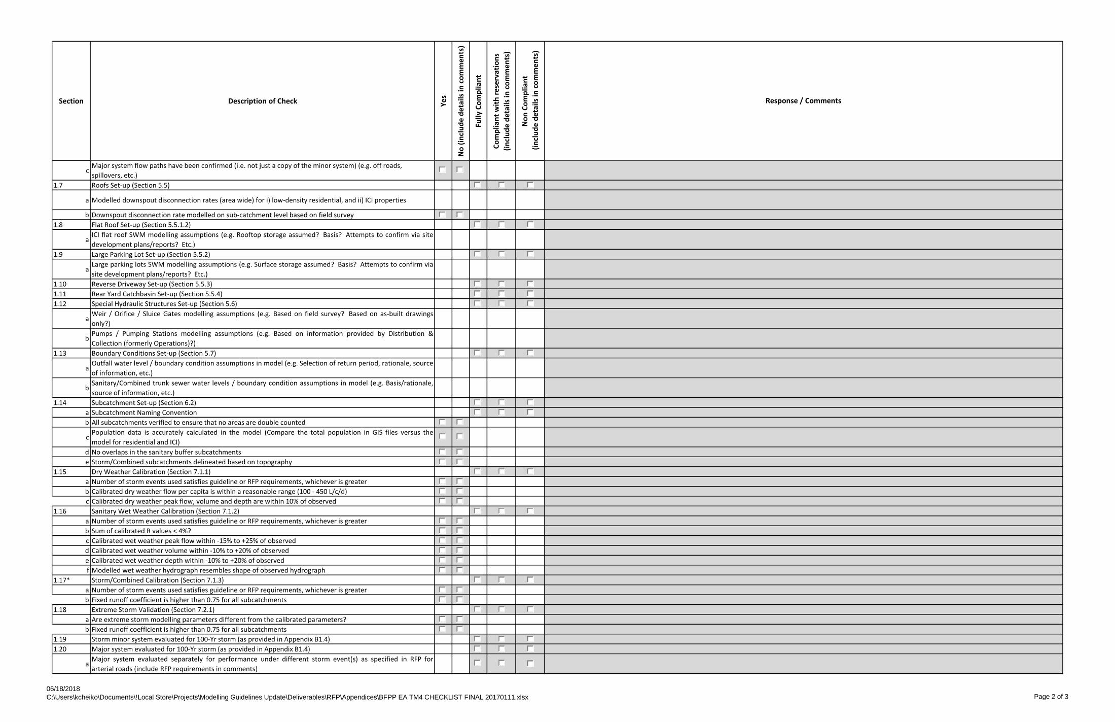
Section Description of Check Yes
No
(in
clu
de
det
ails
in c
om
men
ts)
Fully
Co
mp
lian
t
Co
mp
lian
t w
ith
res
erva
tio
ns
(in
clu
de
det
ails
in c
om
men
ts)
No
n C
om
plia
nt
(in
clu
de
det
ails
in c
om
men
ts)
Response / Comments
cMajor system flow paths have been confirmed (i.e. not just a copy of the minor system) (e.g. off roads,
spillovers, etc.)
1.7 Roofs Set-up (Section 5.5)
a Modelled downspout disconnection rates (area wide) for i) low-density residential, and ii) ICI properties
b Downspout disconnection rate modelled on sub-catchment level based on field survey
1.8 Flat Roof Set-up (Section 5.5.1.2)
aICI flat roof SWM modelling assumptions (e.g. Rooftop storage assumed? Basis? Attempts to confirm via site
development plans/reports? Etc.)
1.9 Large Parking Lot Set-up (Section 5.5.2)
aLarge parking lots SWM modelling assumptions (e.g. Surface storage assumed? Basis? Attempts to confirm via
site development plans/reports? Etc.)
1.10 Reverse Driveway Set-up (Section 5.5.3)
1.11 Rear Yard Catchbasin Set-up (Section 5.5.4)
1.12 Special Hydraulic Structures Set-up (Section 5.6)
aWeir / Orifice / Sluice Gates modelling assumptions (e.g. Based on field survey? Based on as-built drawings
only?)
bPumps / Pumping Stations modelling assumptions (e.g. Based on information provided by Distribution &
Collection (formerly Operations)?)
1.13 Boundary Conditions Set-up (Section 5.7)
aOutfall water level / boundary condition assumptions in model (e.g. Selection of return period, rationale, source
of information, etc.)
bSanitary/Combined trunk sewer water levels / boundary condition assumptions in model (e.g. Basis/rationale,
source of information, etc.)
1.14 Subcatchment Set-up (Section 6.2)
a Subcatchment Naming Convention
b All subcatchments verified to ensure that no areas are double counted
cPopulation data is accurately calculated in the model (Compare the total population in GIS files versus the
model for residential and ICI)
d No overlaps in the sanitary buffer subcatchments
e Storm/Combined subcatchments delineated based on topography
1.15 Dry Weather Calibration (Section 7.1.1)
a Number of storm events used satisfies guideline or RFP requirements, whichever is greater
b Calibrated dry weather flow per capita is within a reasonable range (100 - 450 L/c/d)
c Calibrated dry weather peak flow, volume and depth are within 10% of observed
1.16 Sanitary Wet Weather Calibration (Section 7.1.2)
a Number of storm events used satisfies guideline or RFP requirements, whichever is greater
b Sum of calibrated R values < 4%?
c Calibrated wet weather peak flow within -15% to +25% of observed
d Calibrated wet weather volume within -10% to +20% of observed
e Calibrated wet weather depth within -10% to +20% of observed
f Modelled wet weather hydrograph resembles shape of observed hydrograph
1.17* Storm/Combined Calibration (Section 7.1.3)
a Number of storm events used satisfies guideline or RFP requirements, whichever is greater
b Fixed runoff coefficient is higher than 0.75 for all subcatchments
1.18 Extreme Storm Validation (Section 7.2.1)
a Are extreme storm modelling parameters different from the calibrated parameters?
b Fixed runoff coefficient is higher than 0.75 for all subcatchments
1.19 Storm minor system evaluated for 100-Yr storm (as provided in Appendix B1.4)
1.20 Major system evaluated for 100-Yr storm (as provided in Appendix B1.4)
aMajor system evaluated separately for performance under different storm event(s) as specified in RFP for
arterial roads (include RFP requirements in comments)
06/18/2018
C:\Users\kcheiko\Documents\!Local Store\Projects\Modelling Guidelines Update\Deliverables\RFP\Appendices\BFPP EA TM4 CHECKLIST FINAL 20170111.xlsx Page 2 of 3

Section Description of Check Yes
No
(in
clu
de
det
ails
in c
om
men
ts)
Fully
Co
mp
lian
t
Co
mp
lian
t w
ith
res
erva
tio
ns
(in
clu
de
det
ails
in c
om
men
ts)
No
n C
om
plia
nt
(in
clu
de
det
ails
in c
om
men
ts)
Response / Comments
bMajor system evaluated separately against velocity/depth thresholds as specified in RFP
(include RFP requirements in comments)
1.21 Combined system evaluated for 100-Yr storm (as provided in Appendix B1.4)
1.22 Sanitary system evaluated for May 12, 2000 event (as provied in Appendix B1.4)
1.23 Model Stability (Section 7.3.1)
1.24
No change to simulation parameters from default values. The volume balance is set to 0.01 for initialisation and
simulations
1.25 Correct Design Storms Used for all return period events (Appendix B1.4)
1.26 Any other Modelling Guidelines requirements not explicitly listed above
2 RFP Requirements
2.1
InfoWorks model covers external areas immediately upstream and downstream of the Study Area so that it
allows evaluation of potential hydraulic impacts of the upstream and downstream areas
(indicate in the comments how external areas are incorporated into the model, and the rationale)
2.2The hydrologic and hydraulic models developed for the study area is capable of performing both single event
and continuous simulation on sewersheds consisting of storm, sanitary, and combined sewer systems
2.3A hydrologic and hydraulic model was developed to represent the dual drainage (major and minor) systems for
the storm drainage system of the study area using the agreed-upon version of Infoworks.
2.4Analyze the modeling results in combination with the information gathered for the storm/sanitary and
combined systems to establish possible cause(s) of surface and basement flooding
2.5The validated storm dual drainage model was used to generate flows for ramp-up design storm of 1-, 2-, 5, 10-,
25-, and 100-yr.
2.6A geodatabase / shapefile documenting that the storm sewer capacities for each segment of storm sewer
exceeds or is below the storm events listed (e.g. 100 year, 50-, 25-, 10-, 5-, 2-, 1-year, etc.) has been provided.
2.7 Record of meetings/work session in appendix
2.8
The validated sanitary/combined sewer system model was used to assess the performance of the corresponding
sewer system under major rain storm events, including May 12, 2000, August 19, 2005, July 15, 2012 and July 8,
2013..
2.9The validated sanitary/combined sewer system model was used to generate wet weather flows for ramp-up
design storms of 1-, 2-, 5, 10-, 25-, and 100-yr.
2.10
A geodatabase / shapefile documenting that the storm sewer capacities for each segment of sanitary/combined
sewer exceeds or is below the storm events listed (e.g. 100 year, May 12 2000, 50-,25-, 10-, 5-, 2-, 1-year, etc.)
has been provided.
Notes:
*Additional checklist items related to storm/combined systems may be required
Checklist does not replace meeting requirments as laid out in RFP
06/18/2018
C:\Users\kcheiko\Documents\!Local Store\Projects\Modelling Guidelines Update\Deliverables\RFP\Appendices\BFPP EA TM4 CHECKLIST FINAL 20170111.xlsx Page 3 of 3

06/18/2018
C:\Users\kcheiko\Documents\!Local Store\Projects\Modelling Guidelines Update\Deliverables\RFP\Appendices\tbl_BFPPEA_TM6_checklist_2017-0808.xlsx Page 1 of 3
For Consultants
EA Study TM#6 - Area XX- Checklist Date Reviewed By QA/QC Staff Date Reviewed By Project Manager
RFP No. :
TM# 6 Revision:
Consultant: MM/DD/YYYY
IW Model Version:
Sect
ion
Description of Check Yes
No
(incl
ude
deta
ils in
com
men
ts)
Fully
Com
plia
nt
Com
plia
nt w
ith re
serv
atio
ns
(incl
ude
deta
ils in
com
men
ts)
Non
Com
plia
nt (i
nclu
de d
etai
ls in
com
men
ts)
1 RFP Requirements1.0 Summary of Primary cause(s) of basement and surface flooding identified as presented in TM#41.1 Summary of Basement flooding clusters identified as presented in TM#4
1.2Summary of WQ opportunities for integration with the preferred alternative (based on 2003 WWFMPrecommendations), as presented in TM#5
1.3 The extents (both vertical and horizontal) of potential surface flooding identified
1.4 Water Quality Scenarios Analyzed
a Scenario 1. Existing conditions with future population
bScenario 2. Existing conditions with future population and 75% downspout disconnection (this scenario is onlyrequired if the existing downspout rate is less than 75%)
cScenario 3. Future conditions with basement flooding remediation solutions and 75% downspout disconnectionrate (or existing downspout rate, if higher than 75%)
dScenario 4. Future conditions with basement flooding remediation solutions with applicable water qualitymeasures integrated, applicable WWFMP source/conveyance/EOP controls applied, and 75% downspoutdisconnection rate (or existing downspout rate, if higher than 75%)
e Additional Study Area specific scenarios1.5 Is the MOECC F-5-5 guidleline met for the CSOs in the Study Area?
1.6Was the typical 1991 annual precipitation used for the continuous water quality simulation (as per 2003WWFMP approach, April 1 - October 31)?
1.7 Source vs Conveyance vs End-of-Pipe vs Combination straregies reviewed and preferred strategy selected?
1.8Alternatives developed and evaluated to minimize key potential impacts where the following situations areencountered (provide details in the comment section)
a More than one feasible solution exists to solve the problemb Private property impact and/or easement acquisition requirementsc Impacts to significant number of mature treesd Encroachment on TDSB, TRCA or Parks lands (including playground structures / facilities)e Impacts to TTC streetcar ROWg Major utility conflicts (i.e. major watermains, other sewers)h New outfall is proposedi Operation & Maintenance issues / High O&M Costsj A project that may impact the solution is planned in the vicinity of the Study Area, but not yet constructedk Other situations where an alternative is warranted
1.8Are there any Special Policy Areas (SPAs) or Environmentally Significant Areas (ESAs), as defined in the OfficialPlan within the Study Area?
a Are there any preferred solution located within SPAs? b Can the preferred solutions achieve the BF criteria within the SPAs?
Submission
DRAFT
FINAL
Response / Comments
MM/DD/YYYY MM/DD/YYYY
MM/DD/YYYY MM/DD/YYYY

06/18/2018
C:\Users\kcheiko\Documents\!Local Store\Projects\Modelling Guidelines Update\Deliverables\RFP\Appendices\tbl_BFPPEA_TM6_checklist_2017-0808.xlsx Page 2 of 3
Sect
ion
Description of Check Yes
No
(incl
ude
deta
ils in
com
men
ts)
Fully
Com
plia
nt
Com
plia
nt w
ith re
serv
atio
ns
(incl
ude
deta
ils in
com
men
ts)
Non
Com
plia
nt (i
nclu
de d
etai
ls in
com
men
ts)
Response / Comments
c Are there any preferred solution located within ESAs? 1.9 Cost Estimate
a Was the Cost Estimating Tool (CET) used to develop the cost estimate? Specify the version used in the comments
bWere there items for which the CET did not have a unit cost for? Specify how unit rates for such items wereobtained in the comments
cWas the cost estimate reviewed by the Consultant's cost estimator or an appropriately qualified engineer toconfirm that reasonableness of the cost estimate produced by the CET?
2 Modelling Requirements2.0 Baseline conditions model - future (2041) population used for design, with 450 lpcd applied
2.1Has the peak discharge from sanitary or combined sewers to trunks or sub-trunks leaving the study area underdesign storm in the preferred alternative model remain at the same or lower level than the baseline conditions?
2.2Does the report provide hydrographs to demonstrate that no peak flow increases to the sanitary / combinedtrunk have taken place?
2.3New nodes and conduits proposed as part of alternative solutions are named according to the guidelines (Section 4.5.1.6)
2.4 Data flagging per the guidelines (Section 4.6)2.5 Basement Flooding Design Criteria
aDo all modelled sewer nodes meet the 1.8m HGL freeboard criterion for the design storm (May 12, 2000 for sanitary and 100-Yr for storm and combined systems) in the preferred alternative model?
bDo all modelled overland nodes meet the overland depth criteria for the 100-Yr storm in the preferred alternative model?
cWas the feasibility and practicality of lowering shallow storm sewers investigated and evaluated as an alternative solution where appropriate?
dWhere lowering a shallow storm sewer was not feasible and pipe upgrade has been proposed to eliminate surcharge, is the obvert of the proposed pipe below the obvert of the existing pipe?
eWas a table listing all non-compliant nodes and a justification for non-compliance for each, submitted to the City?
2.6 Compact Transportable Database Submitted to the City
aContaining the "Alternatives" and "Preferred Solution" catchment groups, as outlined in the guidelines (Section 4.5)
2.7 Head Discharge Curves (Section 5.2.2.1)a "ICD_20L" HDT used to represent ICDs (Vortex)b "HCI_250L/s" HDT used to represent High Capacity Inlets
3 Other Requirements3.0 Was an I/I study recommended to be undertaken within the Study Area?
3.1Are there any Basement Flooding solutions within the Study Area that have been proposed by previous adjacent Basement Flooding studies? Provide details in comments section.
3.2 Design Considerationsa Proposed sewer upgrades follow the City's "Design Criteria for Sewers and Watermains"
bAppropriate drops across manholes are used where new sewers are proposed or existing sewers proposed to be upgraded
c No proposed sewers with slope less than the minimum slope requirementsd Proposed pipe sizes conform to commercially availabe pipe sizese Proposed water quality measures are consistent with Wet Weather Flow Management Guidelinesf Proposed water quality measures consider industry standards/guidelines (list documents)
3.3 Constructability Assessment
aWere the alternatives evaluated for conflicts with existing storm, sanitary and combined sewers (minimum clearances achievable)?

06/18/2018
C:\Users\kcheiko\Documents\!Local Store\Projects\Modelling Guidelines Update\Deliverables\RFP\Appendices\tbl_BFPPEA_TM6_checklist_2017-0808.xlsx Page 3 of 3
Sect
ion
Description of Check Yes
No
(incl
ude
deta
ils in
com
men
ts)
Fully
Com
plia
nt
Com
plia
nt w
ith re
serv
atio
ns
(incl
ude
deta
ils in
com
men
ts)
Non
Com
plia
nt (i
nclu
de d
etai
ls in
com
men
ts)
Response / Comments
bWere the alternatives evaluated for conflicts with existing watermains larger than 300mm (minimum clearances achievable)?
cWhere the alternative is located within an easement, has the easement document been received from the Ctiy and reviewed as part of the evaluation process?
d No pipe twinning has been proposede Constructability constraints review for water quality measures (list constraints)
3.4 Inlet Control Devices (ICDs) proposed for less than 20% of total number of catchbasins in the Study Area3.5 Did the stakeholder consultation take place?
a Parks, Facilities, and Recreationb TRCAc Toronto Water Operationsd Transportation Servicese Wastewater and Stormwater Pumpingf Other stakeholders (list in comments field)
3.6 Are any of the following form part of the preferred alternative?a Sanitary off-line storage tanksb Modfications to overland drainagec New outfallsd New trunks or tunnelse Stormwater Management Facilities
3.7 Are any of the solutions impacted by the receiving water course level (Lake Ontario, rivers, creeks)?
Notes:
Checklist does not replace meeting requirments as laid out in RFPChecklist does not constitue an approval list, but rather a guideline indicating some of the content that the City will be looking for in reviewing TM6. The Consultant is still responsible for the accuracy of the deliverables.
*Additional checklist items related to storm/combined systems may be required

Rc_1
Directly Connected Sloped Roof Node (Rc_1)
• Prefix “Rc_”
• System Type = “Storm”
• Elevation 0.6m above receiving street node elevation
• Position as per receiving storm node: x + 3m, y + 2m
• Gully Head-Discharge = "Downspout"
• 1 downspout/65m2 of aggregated roof area
• No storage
ST1
Street Storm Sewer Node (ST1)
• Type = “Storm”
• Gully type & # of gullies based on catchbasin survey
Sloped-Connected Roof Lateral Link (Rc_1.L)
• System Type “Other” to simplify graphics
• Link Suffix = L
• Assumed diameter 300mm (may need to be increased if
S/C is larger than MH-to-MH)
• Assumed length of 30m
• Assumed downstream invert at 1m below receiving
street storm node ground elevation
• Assumed upstream invert at 0.6m above downstream
invert, for 2% slope
Sloped-Connected Roof Overflow Link (Rc_1.U)
• Link Type “User-Control”
• System Type “Overland” to trigger gully
• Link Suffix = U
• Assume spill elevation 0.1m above Directly
Connected Sloped Roof Node elevation
• Head-Discharge Table=“UNLIMITED” to
transfer all spill to Street Storm Node
ST1.1
Directly Connected Sloped Roof Subcatchment (Rc_1)
• Prefix “Rc_”
• System Type “Storm”
• Slope = 0.33% (pitched roof)
• Total Area= Actual topographic ST_1 area
• Contributing = Area of Connected Roof, equal to
the Runoff Surface 30 area
DIRECTLY CONNECTED ROOF SET-UP:
SEPARATED SEWER SYSTEM
ST1.O
Street Storm Link (ST1.1)
• Type = “Storm”
• Link Suffix = increasing numerically from “1”
Street Overland Link (ST1.O)
• Type = “Overland”
• Link Suffix = increasing alphabetically from “O”
ST_1
Topographic Subcatchment (ST_1)
• Prefix “ST_”
• System Type “Storm”
• Runoff Surfaces to include 10, 20
and 50 series
SA_1
SP_1
Sanitary Subcatchments (SA_1)
• Prefix “SA_”; Buffer-based GWI/WWF flow
• System Type “Other”
Sanitary Subcatchments (SP_1)
• Prefix “SP_”; Parcel-based sewage flow
• System Type “Sanitary”
Rc_1
S1.1
Street Sanitary Link (S1.1)
• Type = “Sanitary”
• Link Suffix = increasing numerically from “1”
S1

Rc_1
Rc_1
Directly Connected Sloped Roof Node (Rc_1)
• Prefix “Rc_”
• System Type = “Storm”
• Elevation 0.6m above receiving street node elevation
• Position as per receiving storm node: x + 3m, y + 2m
• Gully Head-Discharge = "Downspout"
• 1 downspout/65m2 of aggregated roof area
• No storage
CO1
Street Combined Sewer Node (CO1)
• Type = “Combined”
• Gully type & # of gullies based on catchbasin survey
Sloped-Connected Roof Lateral Link (Rc_1.L)
• System Type “Other” to simplify graphics
• Link Suffix = L
• Assumed diameter 300mm (may need to be increased if
S/C is larger than MH-to-MH)
• Assumed length of 30m
• Assumed downstream invert at 1m below receiving
street combined node ground elevation
• Assumed upstream invert at 0.6m above downstream
invert, for 2% slope
Sloped-Connected Roof Overflow Link (Rc_1.U)
• Link Type “User-Control”
• System Type “Overland” to trigger gully
• Link Suffix = U
• Assume spill elevation 0.1m above Directly
Connected Sloped Roof Node elevation
• Head-Discharge Table=“UNLIMITED” to
transfer all spill to Street Combined Node
CO1.1
Directly Connected Sloped Roof Subcatchment (Rc_1)
• Prefix “Rc_”
• System Type “Storm”
• Slope = 0.33% (pitched roof)
• Total Area= Actual topographic ST_1 area
• Contributing = Area of Connected Roof, equal to
the Runoff Surface 30 area
CO1.O
Street Combined Link (CO1.1)
• Type = “Combined”
• Link Suffix = increasing numerically from “1”
Street Overland Link (ST1.O)
• Type = “Overland”
• Link Suffix = increasing alphabetically from “O”
• Defined cross-section based on road width
ST_1
Topographic Subcatchment (ST_1)
• Prefix “ST_”
• System Type “Storm”
• Runoff Surfaces to include 10, 20
and 50 series
DIRECTLY CONNECTED ROOF SET-UP:
COMBINED SEWER SYSTEM
Sanitary Subcatchments (SA_1)
• Prefix “SA_”; Buffer-based GWI/WWF flow
• System Type “Other”
Sanitary Subcatchments (SP_1)
• Prefix “SP_”; Parcel-based sewage flow
• System Type “Sanitary”
SA_1
SP_1

CO1.1
Rc_1
Rc_1
Directly Connected Sloped Roof Node (Rc_1)
• Prefix “Rc_”
• System Type = “Storm”
• Elevation 0.6m above receiving street node elevation
• Position as per receiving storm node: x + 3m, y + 2m
• Gully Head-Discharge = "Downspout"
• 1 downspout/65m2 of aggregated roof area
• No storage
CO1
Street Sewer Nodes (ST1 & CO1)
• ST1 is of Type = “Storm”; Gully type & # of gullies based
on catchbasin survey
• CO1 is of Type = “Combined”; Gully type dependent on
MH cover survey (perforated, 2-pick holes)
• Interconnect with Overland link where critical (low point)
Sloped-Connected Roof Lateral Link (Rc_1.L)
• System Type “Other” to simplify graphics
• Link Suffix = L
• Assumed diameter 300mm (may need to be increased)
• Assumed length of 30m
• Assumed downstream invert at 1m below receiving
street Combined node ground elevation
• Assumed upstream invert at 0.6m above downstream
invert, for 2% slope
Sloped-Connected Roof Overflow Link (Rc_1.U)
• Link Type “User-Control”
• System Type “Overland” to trigger gully
• Link Suffix = U
• Assume spill elevation 0.1m above Directly
Connected Sloped Roof Node elevation
• Head-Discharge Table=“UNLIMITED” to
transfer all spill to Street Storm Node
Directly Connected Sloped Roof Subcatchment (Rc_1)
• Prefix “Rc_”
• System Type “Storm”
• Slope = 0.33% (pitched roof)
• Total Area= Actual topographic ST_1 area
• Contributing = Area of Connected Roof, equal to
the Runoff Surface 30 area
ST1.O
Street Combined Link (CO1.1)
• Type = “Combined”
• Link Suffix = increasing numerically from “1”
Street Overland Link (ST1.O)
• Type = “Overland”
• Link Suffix = increasing alphabetically from “O”
ST_1
Topographic Subcatchment (ST_1)
• Prefix “ST_”
• System Type “Storm”
• Runoff Surfaces to include 10, 20
and 50 series
DIRECTLY CONNECTED ROOF SET-UP:
COMBINED w/ ROAD STORM SEWER
Sanitary Subcatchments (SA_1)
• Prefix “SA_”; Buffer-based GWI/WWF flow
• System Type “Other”
Sanitary Subcatchments (SP_1)
• Prefix “SP_”; Parcel-based sewage flow
• System Type “Sanitary”
SA_1
SP_1ST1
ST1.1 Street Storm Link (ST1.1)
• Type = “Storm”
• Link Suffix = increasing numerically from “1”

FRc_1
Directly Connected Flat Roof Node (FRc_1)
• Prefix “FRc_”
• System Type = “Storm”
• Elevation 0.6m above receiving street node elevation
• Position as per receiving storm node: x + 6m, y + 4m
• Gully Head-Discharge = “FlatRoof"
• 1 roof drain/160m2 of aggregated flat roof area
• Storage Parameters assume 80% of flat roof area, and
a Max depth 0.05m of storage before spill
ST1 Street Storm Sewer Node (ST1)
• Type = “Storm”
• Gully type & # of gullies based on catchbasin survey
Flat Roof Lateral Link (FRc_1.L)
• System Type “Other” to simplify graphics
• Link Suffix = L
• Assumed diameter 300mm (may need to be increased if
large flat roof area)
• Assumed length of 30m
• Assumed downstream invert at 1m below receiving
street storm node ground elevation
• Assumed upstream invert at 0.6m above downstream
invert, for 2% slope
Connected Flat Roof Overflow Link (FRc_1.U)
• Link Type “User-Control”
• System Type “Overland” to trigger gully
• Link Suffix = U
• Assume spill elevation 0.05m above Flat Roof
Node elevation
• Head-Discharge Table=“UNLIMITED” to
transfer all spill to Street Storm Node
ST1.1
Directly Connected Flat Roof Subcatchment (FRc_1)
• Prefix “FRc_”
• System Type “Storm”
• Slope = 0.001% (flat roof)
• Total Area= Actual topographic ST_1 area
• Contributing = Area of Connected Roof, equal to
the Runoff Surface 40 area
DIRECTLY CONNECTED FLAT ROOF
SET-UP: SEPARATED SEWER SYSTEM
ST1.O
Street Storm Link (ST1.1)
• Type = “Storm”
• Link Suffix = increasing numerically from “1”
Street Overland Link (ST1.O)
• Type = “Overland”
• Link Suffix = increasing alphabetically from “O”
ST_1
Topographic Subcatchment (ST_1)
• Prefix “ST_”
• System Type “Storm”
• Runoff Surfaces to include 10, 20
and 50 series
FRc_1

FRd_1
Disconnected Flat Roof Node#1 (FRd_1)
• Prefix “FRd_”
• System Type = “Storm”
• Elevation 0.8m above receiving street node elevation
• Position as per receiving storm node: x + 11m, y + 5m
• Gully Head-Discharge = “FlatRoof"
• 1 roof drain/160m2 of aggregated flat roof area
• Storage Parameters assume 80% of flat roof area, and
a Max depth 0.05m of storage before spill
ST1
Disconnected Flat Roof Flow Link (FRd_1!.O)
• Link Type “Conduit”
• System Type “Overland” to connect to street overland
• Link Suffix = O
• Cross-Section = “OREC”
• Width = 20000mm width, Height = 300mm
• Length = 5m (slope will be 6%)
ST1.1
Disconnected Flat Roof Subcatchment (FRd_1)
• Prefix “FRd_”
• System Type “Storm”
• Slope = 0.001% (flat roof)
• Total Area= Actual topographic ST_1 area
• Contributing = Area of Connected Roof, equal to
the Runoff Surface 40 area
DISCONNECTED FLAT ROOF SET-UP:
SEPARATED SEWER SYSTEM
ST1.O
Street Overland Link (ST1.O)
• Type = “Overland”
• Link Suffix = increasing alphabetically from “O”
ST_1
Topographic Subcatchment (ST_1)
• Prefix “ST_”
• System Type “Storm”
• Runoff Surfaces to include 10, 20
and 50 series
FRd_1
Disconnected Flat Roof Node#2 (FRd_1!)
• Add “!” to “FRd_#” ID
• System Type = “Overland”, Node Type “Sealed”
• Elevation 0.3m above receiving street node elevation
• Position as per receiving storm node: x + 9m, y + 5m
FRd_1!
RFd_1.U
Street Storm Sewer Node (ST1)
• Type = “Storm”
• Gully type & # of gullies based on catchbasin survey
Street Storm Link (ST1.1)
• Type = “Storm”
• Link Suffix = increasing numerically from “1”
Connected Flat Roof Conveyance Link (FRd_1.U)
• Link Type “User-Control”
• System Type “Storm”
• Link Suffix = U
• Used to convey flow to overland channel (to
not bypass the street gully)
• Assume elevation 0.29m below Flat Roof
Node#1 elevation
• Head-Discharge Table=“UNLIMITED”

APPENDIX E.12
Code of Practice for the Hydraulic Modelling of Urban Drainage Systems 2017
(Chartered Institution of Water and Environmental Management CIWEM Urban Drainage Group)

i
CIWEM UDG CODE OF PRACTICE FOR THE HYDRAULIC MODELLOING OF URBAN DRAINAGE SYSTEMS 2017
Urban Drainage Group
Code of Practice for the Hydraulic Modelling of Urban Drainage Systems
Version 01

i
CIWEM UDG CODE OF PRACTICE FOR THE HYDRAULIC MODELLOING OF URBAN DRAINAGE SYSTEMS 2017
Code of Practice for the Hydraulic Modelling of Urban Drainage Systems 2017.
www.ciwem.org/groups/udg
Technical enquiries
All technical enquiries and suggestions relating to this publication should be addressed to the Urban Drainage Group mailbox: [email protected].
The Code of Practice is issued for guidance in good faith following extensive industry consultation. CIWEM cannot accept responsibility for consequences arising from its application. It is intended that the Code of Practice will undergo periodic review to reflect good practice and new technologies as they mature.
This entire document may be freely copied provided that the text is reproduced in full, the source acknowledged and provided it is not sold.
Version Control
Version Number Description Date 01 First release to industry 3rd November 2017
Acknowledgments
Authors
Version 1 of this guidance was written by an industry team:
John Titterington MWH now part of Stantec
Graham Squibbs MWH now part of Stantec
Chris Digman MWH now part of Stantec
Richard Allitt RAA
Martin Osborne WSP
Paul Eccleston JBA
Alan Wisdish Atkins

ii
CIWEM UDG CODE OF PRACTICE FOR THE HYDRAULIC MODELLOING OF URBAN DRAINAGE SYSTEMS 2017
Project Steering Group
The project was carried out with the guidance and assistance of the Project Steering Group Members, their representatives and colleagues as follows:
Keith Kipling (Chair) CIWEM UDG and United Utilities
Elliot Gill (Co-Chair) CIWEM and CH2M
Ed Bramley (Co-Chair) CIWEM and Yorkshire Water
Nadia Peters Anglian Water
Phil Hulme Environment Agency
Francis Finnerty Irish Water
Nicola Hyslop Northumbrian Water
Bob Flemming Scottish Water
Mark McLaughlin SEPA
David Terry Severn Trent Water
Marc Barton Southern Water
Andrew Hagger Thames Water
Steve Kenney United Utilities
David Ripley Welsh Water
David Searby Wessex Water
Mark Russell Yorkshire Water
CIWEM also thank the Water Environment Federation (WEF) -Collection Systems Committee Technical Practice Group for their comments.
CIWEM is the leading independent Chartered professional body for water and environmental professionals, promoting excellence within the sector.
© November 2017. The Chartered Institution of Water and Environmental Management (CIWEM).
106 to 109 Saffron Hill, Farringdon, London, EC1N 8QS. Tel: 020 7813 3110.
Charity Registration No. 1043409 (England and Wales) SCo38212 (Scotland)

iii
CIWEM UDG CODE OF PRACTICE FOR THE HYDRAULIC MODELLOING OF URBAN DRAINAGE SYSTEMS 2017
Contents
1 INTRODUCTION ............................................................................................................................................... 1
1.1 Purpose of the Code of Practice ....................................................................................................... 1
1.2 Terminology and language ................................................................................................................ 1
1.3 Target audience ...................................................................................................................................... 1
1.4 Stakeholders ............................................................................................................................................. 1
1.5 Experience and training of staff ........................................................................................................ 2
1.6 Applying the Code of Practice........................................................................................................... 2
2 PROJECT DEFINITION .................................................................................................................................... 6
2.1 Scope and context ................................................................................................................................. 6
2.2 Purpose and drivers............................................................................................................................... 6
2.3 Defining, assessing and measuring model confidence............................................................ 7
2.4 Types of model use and levels of detail ........................................................................................ 7
2.5 Modelling boundary conditions and interactions ................................................................... 10
2.6 Assessing existing models ................................................................................................................ 11
2.7 Documentation ..................................................................................................................................... 11
3 DATA REQUIREMENTS AND DATA COLLECTION ............................................................................. 12
3.1 Introduction ............................................................................................................................................ 12
3.2 Principles for data collection ............................................................................................................ 13
3.3 Partnership working ............................................................................................................................ 13
3.4 Planning Data Collection ................................................................................................................... 14
3.5 Survey guidance ................................................................................................................................... 17
3.6 Existing models ..................................................................................................................................... 17
3.7 Drainage asset data ............................................................................................................................. 18
3.8 Hydrological and topographic data .............................................................................................. 18
3.9 Dry Weather and Base Flow ............................................................................................................. 21
3.10 Flow data collection and surveys ................................................................................................... 23
3.11 Operational Data .................................................................................................................................. 33
3.12 Non-quantitative data sources ....................................................................................................... 34
3.13 Mapping data, aerial photography and street mapping ....................................................... 35
3.14 Data confidentiality ............................................................................................................................. 35
4 MODEL DEVELOPMENT .............................................................................................................................. 36
4.1 Introduction ............................................................................................................................................ 36
4.2 Defining the model catchment and subcatchments ............................................................... 41
4.3 Drainage system model ..................................................................................................................... 50

iv
CIWEM UDG CODE OF PRACTICE FOR THE HYDRAULIC MODELLOING OF URBAN DRAINAGE SYSTEMS 2017
4.4 Flood modelling / modelling surface flows ................................................................................ 61
4.5 Modelling operational issues ........................................................................................................... 65
4.6 Model testing / sense checks .......................................................................................................... 67
5 MODEL VERIFICATION ................................................................................................................................ 70
5.1 Introduction ............................................................................................................................................ 70
5.2 Verification procedure ........................................................................................................................ 71
5.3 Verification with flow data ................................................................................................................ 71
5.4 Verification with historical data ...................................................................................................... 75
5.5 Dealing with none-achievement of verification targets ........................................................ 77
6 ASSESSING MODEL CONFIDENCE .......................................................................................................... 78
6.1 Introduction to assessing model confidence............................................................................. 78
6.2 Developing and applying a model confidence assessment ................................................. 78
6.3 Visualising and using confidence in spatial units .................................................................... 85
6.4 Weightings of categories and “Fit for use” review .................................................................. 85
7 Application of Models ................................................................................................................................. 86
7.1 Introduction ............................................................................................................................................ 86
7.2 Model Review ........................................................................................................................................ 86
7.3 Model preparation ............................................................................................................................... 87
7.4 Boundary conditions ........................................................................................................................... 91
7.5 Rainfall ...................................................................................................................................................... 93
7.6 Assessment of hydraulic and environmental performance .................................................. 94
7.7 Developing the model for real time data, live running and forecasting ......................... 94
7.8 Documentation ..................................................................................................................................... 95
8 DOCUMENTATION ....................................................................................................................................... 96
8.1 Introduction ............................................................................................................................................ 96
8.2 Model Definition Documentation .................................................................................................. 96
8.3 Data Collection Documentation ..................................................................................................... 97
8.4 Model development ............................................................................................................................ 98
8.5 Model Verification and Confidence Documentation .............................................................. 99
8.6 Model Application ............................................................................................................................ 100
8.7 Quality assurance and review including audit ........................................................................ 100
9 MODEL MANAGEMENT ........................................................................................................................... 101
9.1 Introduction ......................................................................................................................................... 101
9.2 Model libraries.................................................................................................................................... 101
9.3 When to update or maintain models ........................................................................................ 102

v
CIWEM UDG CODE OF PRACTICE FOR THE HYDRAULIC MODELLOING OF URBAN DRAINAGE SYSTEMS 2017
APPENDICES .......................................................................................................................................................... 104
APPENDIX A – EXAMPLES OF DEFINING MODEL CONFIDENCE LEVELS ....................................... 105
APPENDIX B – ITEMS TO CONSIDER FOR A MODEL ASSESSMENT OR MODEL AUDIT ........... 107
APPENDIX C – DATA COLLECTION LEVELS ................................................................................................ 108
APPENDIX D - ASSET DATA COLLECTION ................................................................................................. 115
APPENDIX E Runoff Models ............................................................................................................................ 126
APPENDIX F - SCATTERGRAPHS .................................................................................................................... 128
APPENDIX G – EXAMPLE OF STATISITICAL METHOD FOR STORM VERIFICATION: THE NASH-SUTCLIFFE EFFICIENCY COEFFICIENT ........................................................................................................... 132
APPENDIX H – EXAMPLE APPROACH TO DRY WEATHER VERIFICATION ..................................... 133
APPENDIX I –EXAMPLE OF APPLYING THE NASH-SUTCLIFFE EFFICIENCY COEFFICIENT FOR STORM VERIFICATION ....................................................................................................................................... 136
APPENDIX J – EXAMPLE OF QUALITATIVE SCORING APPROACH .................................................... 138
APPENDIX K – EXAMPLE OF NUMERICAL SCORING APPROACH ..................................................... 143
APPENDIX L: Types of Intervention ............................................................................................................... 148
REFERENCES AND BIBLIOGRAPHY ................................................................................................................ 149
GLOSSARY & ABBREVIATIONS ....................................................................................................................... 151

1
CIWEM UDG CODE OF PRACTICE FOR THE HYDRAULIC MODELLOING OF URBAN DRAINAGE SYSTEMS 2017
1 INTRODUCTION
1.1 Purpose of the Code of Practice
The Code of Practice (CoP) is intended to be a good practice guide to the hydraulic modelling of urban drainage systems. It is primarily based on the modelling practices in the UK and Ireland, and if used outside this geographic area the user must apply judgement in adapting this to local conditions and practices.
The CoP is not software specific, although some examples may use a particular software product. It should be noted that the choice of software to use must be commensurate with the required confidence in the modelling outputs.
It is not intended to be used directly as a specification for modelling and Commissioning Bodies should consider the development of their own more detailed specifications.
1.2 Terminology and language
The CoP uses language and terms predominantly related to the United Kingdom and Ireland, although the practices outlined will be relevant for use internationally. A glossary of terms is included to aid the user who is not familiar with these
1.3 Target audience
The target audience is urban drainage practitioners who are actively involved in the commissioning, development, use and maintenance of hydraulic models in the urban environment. In particular this will include the Commissioning Body, the organisation who commissions the work and the Modelling Team, those who undertake the modelling work. Examples of a Commissioning Body could be a Government Department, Water Company or a Local Authority. In this CoP, reference is made to the Modelling Team as the ‘Modeller’ for ease of reference, but may refer to the team or an individual from the team.
1.4 Stakeholders
A number of stakeholders may have an interest in urban drainage modelling projects. This may include the needs and outcomes of the project, the provision of data to the project, output from the project in a particular format or for a potential future use of the modelling tools developed.
It is necessary to understand how different stakeholders are involved and interact as part of an Urban Drainage Project and how the needs of customers are considered. This should include the impact on the public as the ultimate customers of urban drainage projects.
The stakeholders to be considered include (but are not restricted to):
• External Stakeholders – Government, Regulators, Water Companies, Lead Local Flood Authorities, Local Authorities, Internal Drainage Boards, etc.
• Internal Stakeholders – Any internal department with a responsibility for an aspect of a project (e.g. Asset Planners, Operations Teams)

2
CIWEM UDG CODE OF PRACTICE FOR THE HYDRAULIC MODELLOING OF URBAN DRAINAGE SYSTEMS 2017
• Customers and Communities – Should consider all aspects of potential customer interaction through Consumer Organisations (e.g. Council for Water), Local Customer Action Groups, Domestic and Commercial Customers, etc.
• Pressure Groups
It is good practice to develop a Stakeholder Management Plan, identifying systematically the relative importance of stakeholders to the project, and setting out a plan of action to communicate with, engage with and reflect concerns of stakeholders.
1.5 Experience and training of staff
Urban drainage modelling has always been a complex subject and, with more integration of systems and improvements in technology, it is continually becoming more complex. It is essential, therefore, that all staff involved in the work should have received training appropriate to the tasks they are carrying out. This CoP is not a substitute for such training. Training may be as part of formal education, by in-house or external training courses, open learning or on-the-job training. Records should be kept of the training individuals have received.
Work should be carried out by, or under the day to day direction of, a competent hydraulic modeller who should have a detailed understanding of drainage and sewerage systems and the various processes involved, including (but not limited to):
• Operational performance requirements for urban drainage systems
• Hydraulics of flow in sewers, sustainable drainage systems, watercourses and ancillary structures
• Urban hydrology
• The assumptions implicit in the way the software carries out the calculations
• Methods of flow measurement and their accuracy
• Engineering solutions
The CIWEM Urban Drainage Group (UDG) Competency Framework provides a framework for defining the competency requirements of staff involved in a project, and assessing individual staff competencies against those requirements.
1.6 Applying the Code of Practice
1.6.1 What it covers
The CoP covers the hydraulic modelling of both the underground piped drainage systems and the above ground systems, together with their interaction in the urban environment. The below ground systems are typically made up of sewers but could also be culverted watercourses or highway drains. The above ground systems would include watercourses that form the principal drainage pathways for catchments and the overland flow paths on river flood plains and the urban environment. Elements of the integration of the two systems are considered more fully in the CIWEM UDG (2009) Integrated Modelling Guide.

3
CIWEM UDG CODE OF PRACTICE FOR THE HYDRAULIC MODELLOING OF URBAN DRAINAGE SYSTEMS 2017
The CoP does not cover the non-hydraulic elements of water quality modelling, water quality aspects of the impact of urban discharges on the receiving watercourse, or the development of standalone watercourse models for flood risk management purposes.
1.6.2 Modelling process
Figure 1-1 shows a typical high-level sequence of the processes involved in the development of Urban Drainage Models, and this CoP covers all these aspects. Although this shows a linear process, some tasks may run in parallel, such as building or updating a model may occur at the same time as undertaking the flow survey.
Section 8 of the CoP covers documentation for all the sections of the Code. . It should be noted however that the review and documentation process is an ongoing activity which should be carried out throughout the development of the project and not left to the end.
1.6.3 Aligning with other practice
This Code of Practice is not a standalone document and forms part of a suite of CIWEM UDG documents. It should be read in conjunction with the following CIWEM UDG documents:
Essential:
• Rainfall Modelling Guide 2016, Version 1.0 March 2016
• Integrated Urban Drainage Modelling Guide 2009, V01-001 June 2009
• Competency Framework, Draft November 2015
• Event Duration Monitoring Good Practice Guide, Version 2.2 January 2016
• CIWEM UDG User Notes:
o User Note 1 – Modelling Vortex Flow Control devices, Version 4, (2009) o User Note 2 – Modelling ancillaries and discharge coefficients, Version 3,
(2009) o User Note 13 – The dangers of force fitting, version3, (2009). o User Note 15 – Storage Compensation, version 3, (2009). o User Note 22 – Selection of tide levels, version 3, (2009) o User Note 27 – Modelling ancillaries: weir coefficients, version 2, (2009) o User Note 28 – A new runoff model, version3, (2009) o User Note 33 – Modelling dry weather flow, version 2, (2009)
More relevant for Urban Pollution Management (UPM) and water quality modelling by CIWEM DUG:
• Guide To The Quality Modelling Of Sewer Systems, Version 1.0 November (2006)
• River Modelling Guide, Version W01 November (1999)
• River Data Collection Guide, Version W01 November (1999)

4
CIWEM UDG CODE OF PRACTICE FOR THE HYDRAULIC MODELLOING OF URBAN DRAINAGE SYSTEMS 2017
In addition, there are a number of other significant external publications, some of which are listed as follows:
• C635 Designing for Exceedance in Urban Drainage - Good Practice, (CIRIA, 2006)
• C753 The SUDS Manual, (CIRIA, 2015)
• Drainage Strategy Framework, (Ofwat/EA 2013)
• Flood Estimation Handbook (FEH), issued in a set of five printed volumes (Centre for Ecology & Hydrology, 1999)
• Flood Modelling Guidance for Responsible Authorities Version 1.1, (SEPA, 2017)
• Sewerage Risk Management (SRM), (WRc, 2017)
• Sewers for Adoption 7th Edition, (WRc, 2012)
• Sewers for Scotland 3rd Edition, (Scottish Water & WRc, 2015)
• Surface Water Management Plan Technical Guidance, (Defra, 2010)
• The Fluvial Design Guide, (Environment Agency, 2010)
• Urban Pollution Management (UPM) Manual, (FWR, 2012)
If there is any discrepancy between this Code of Practice and other CIWEM UDG documents, the Code of Practice will take priority unless the CIWEM UDG documents post-date this Code of Practice.
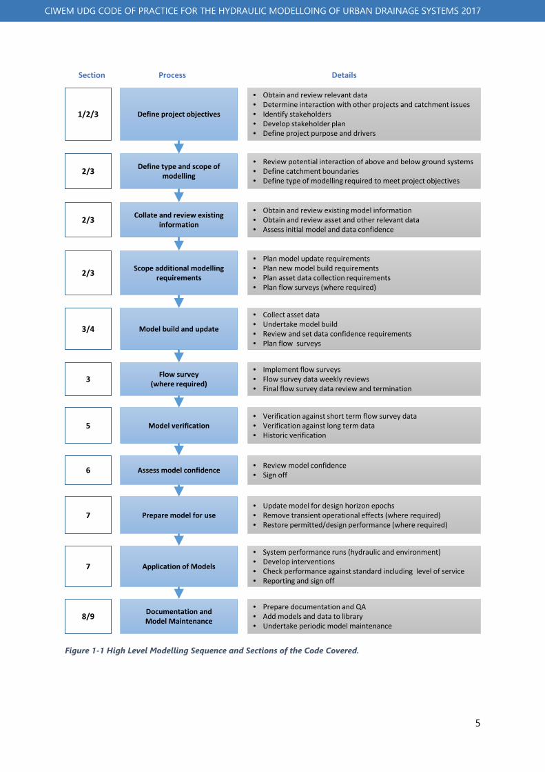
5
CIWEM UDG CODE OF PRACTICE FOR THE HYDRAULIC MODELLOING OF URBAN DRAINAGE SYSTEMS 2017
Figure 1-1 High Level Modelling Sequence and Sections of the Code Covered.
Define project objectives1/2/3
Section Process Details
• Obtain and review relevant data• Determine interaction with other projects and catchment issues• Identify stakeholders• Develop stakeholder plan• Define project purpose and drivers
Define type and scope of modelling2/3
• Review potential interaction of above and below ground systems• Define catchment boundaries• Define type of modelling required to meet project objectives
Collate and review existing information 2/3
• Obtain and review existing model information• Obtain and review asset and other relevant data• Assess initial model and data confidence
Scope additional modelling requirements2/3
• Plan model update requirements• Plan new model build requirements• Plan asset data collection requirements• Plan flow surveys (where required)
Model build and update3/4
• Collect asset data• Undertake model build• Review and set data confidence requirements• Plan flow surveys
Flow survey (where required)3
• Implement flow surveys• Flow survey data weekly reviews• Final flow survey data review and termination
Model verification5• Verification against short term flow survey data• Verification against long term data• Historic verification
Assess model confidence6 • Review model confidence• Sign off
Prepare model for use7• Update model for design horizon epochs• Remove transient operational effects (where required)• Restore permitted/design performance (where required)
Application of Models7
• System performance runs (hydraulic and environment)• Develop interventions• Check performance against standard including level of service• Reporting and sign off
Documentation andModel Maintenance8/9
• Prepare documentation and QA• Add models and data to library• Undertake periodic model maintenance

6
CIWEM UDG CODE OF PRACTICE FOR THE HYDRAULIC MODELLOING OF URBAN DRAINAGE SYSTEMS 2017
2 PROJECT DEFINITION
2.1 Scope and context
This section covers the scoping of modelling projects, including defining the project purpose and drivers, the types of models required and the confidence in the output required for the project. The process for this section is outlined Figure 2-1.
Figure 2-1 Project Definition Overview
2.2 Purpose and drivers
Before embarking on producing a hydraulic model the purpose and required use of the model should be clearly defined.
There are numerous potential reasons for requiring a model, including, but not limited to models needed for general planning purposes, operational use, development control, problem investigation and detailed design of interactions. In each case there is potential for differing requirements in terms of modelling techniques, standards of data collection, modelling detail and verification, leading to varying levels of model confidence.
It is therefore necessary to define the information required from the model, the points at which this information is required and the confidence required in the modelled outputs. The responsibility for defining this would normally rest with the Commissioning Body as the ultimate user and custodian of the completed model, after taking account of the requirements of key stakeholders. In some instances there may be a need for approval of the modelling scope by others, for example by an environmental regulator for a model to be
Understand Purpose and Drivers
Level of Detail for Types of Model Use
Modelling Boundary Conditions and Interactions
Defining, Assessing and Measuring Confidence
Assessing Existing Models
Documentation
Section 3 - Data evaluation
Section 4 – Sub catchment definition
Appendix 2BSection 7 – Use of Models
Section 8.2 – Model Definition Documentation
Appendix 2ASection 3 – Data Collection
Section 5 – Model VerificationSection 6 – Model Confidence
2.2
2.3
2.4
2.5
2.6
2.7
Section Process Related sections

7
CIWEM UDG CODE OF PRACTICE FOR THE HYDRAULIC MODELLOING OF URBAN DRAINAGE SYSTEMS 2017
used for an assessment of the impact of intermittent discharges on the receiving environment.
2.3 Defining, assessing and measuring model confidence
There is a degree of uncertainty in many aspects relating to modelling. The list of areas of uncertainty is large, given the number of data inputs and the complex numerical calculations that transfer physical processes into a mathematical form.
Over the years modelling practice has developed to attempt to manage these uncertainties, by developing standards for significant elements of the modelling process for both inputs and outputs to provide some level of confidence in the modelled outputs.
There are five main categories to consider when assessing and measuring confidence. These are:
• Asset data, including real time controls (RTC)
• Subcatchment data
• Flow data
• Flow verification
• Historical verification
Each of these areas will have varying levels of confidence, dependent on the level of detail, accuracy and amount of data used in the model. As a general rule the more surveyed data are used in the model, either from physical surveys or from other reliable sources, the higher the model confidence.
It is important that the Commissioning Body defines the required confidence levels for the specific purpose. Setting the levels too high will result in an unduly expensive model whereas levels set too low may result in a model that does not meet expectations. In most instances budget constraints will have to be taken into account in defining the data collection and verification requirements.
The level of detail required for data collection is considered further in Section 3 of the CoP, and verification is considered further in Section 5 and associated appendices. Section 6 and associated appendices provides a framework for confidence to be assessed in a qualitative or quantitative approach.
It is unlikely that there will be a need for a uniform standard of confidence across the whole model. As a Commissioning Body, there will be a need to determine the areas (zones) or elements of the model that require a higher level of confidence, for example in an area of reported flooding or a CSO discharge known to be impacting on the receiving environment with a potential for a scheme. Appendix A provides examples of defining model confidence levels qualitatively in different parts of a catchment, and the level of detail for different types of use are considered below.
2.4 Types of model use and levels of detail
Models are likely to be defined based on their purpose and following a convention that considers four principal aspects of the model:

8
CIWEM UDG CODE OF PRACTICE FOR THE HYDRAULIC MODELLOING OF URBAN DRAINAGE SYSTEMS 2017
• The level of detail of the model
• What parameters are modelled? This is limited to hydraulic only in the CoP
• The number of dimensions in which the modelling is undertaken
• The hydrology which has been used in the model
All types of models may contain elements of both the above and below ground drainage systems but the general principles apply in all situations. The CoP provides some guidance for modelling watercourses but other documentation should be consulted as outlined in Section 1.6.3.
2.4.1 Level of detail of elements of the model
The level of detail will generally fall within one of the following categories:
• Type I – limited detail, simplified, typically used in locations to gain an appreciation of performance or to represent the transfer flows to a more detailed part of the model
• Type II – planning, general purpose, typically used in locations to understand risk
• Type III – high level of detail, typically used in locations for detailed investigation and design
Many models built or updated will be a “Hybrid” of the three levels, i.e. they will have a varying level of detail in specific areas or in relation to certain types of assets or features, as detailed in the project scope.
Models typically have two components. These are:
• Flow generation: sub catchment definition or direct runoff to give the parameters that are used to generate the flow (foul, surface water runoff, etc.)
• Physical details: definition of the assets (manholes, pipes, channels, flow paths, ancillary structures, active controls etc.)
As models are generally built from GIS based sewer record databases there has been a progression in the industry towards “all pipe models”. These are built from existing records and therefore they will typically be a Type II level of detail.
More information is provided in sections 4.2 and 4.3
2.4.1.1 Type I - Simplified
As its name implies, it is a highly simplified representation of the modelled system. Typically, this type will have specific objectives related to the whole catchment or applied to part of a large catchment. The specific objectives of this type of model detail could include providing:
• A simulation of the flows and conditions at one or more specific locations (e.g. sea outfall, pumping station, treatment works)
• A simulation of the boundary conditions in a trunk sewer, an intercepting sewer or a watercourse so that more detailed models of connecting sewer systems or smaller watercourses can be modelled with the correct tailwater conditions, etc.
• A simple framework model of a network into which a detailed model can be incorporated, obviating the need for boundary conditions to be deduced
9
CIWEM UDG CODE OF PRACTICE FOR THE HYDRAULIC MODELLOING OF URBAN DRAINAGE SYSTEMS 2017
• A reasonably accurate representation of a trunk sewer system, an intercepting sewer system or a watercourse without needing to model exactly the layout of tributaries or contributing sewer networks
• The backbone of a rapid simulation model such as one that might be required for flood forecasting purposes
Flow generation will typically be based on sewer records with no contributing area site surveys, and subcatchments would tend to be larger than in more detailed models.
This type of model detail is not adequate for detailed modelling or for general planning purposes.
2.4.1.2 Type II – Planning Type
This type of model detail is considered as “general multi-purpose”. This would typically be the default type of model in the absence of any specific requirements.
This provides an overview of a specific drainage area, which might be a discrete catchment in its own right or may be part of a larger catchment. The purpose of this type of model detail for hydraulic purposes is primarily as a planning or assessment tool to:
• Identify hydraulic problems within a drainage area, including the identification of flooding risks, surcharged pipes, throttles, reverse flows
• Simulate and identify the performance of Combined Sewer Overflows and other ancillaries
• Identify the need for possible hydraulic upgrading schemes and to carry out initial scheme appraisals
• Assess the impact of proposed developments, climate change and urban creep
Type II model detail should include all significant ancillaries (although small pumping stations may be omitted) and typically all known problem areas, particularly those of known flooding or surcharge. Simplification of the network in the model is not normally undertaken, although consideration could be given to trimming smaller diameter sewers of 150mm or below from the model, ensuring that all low lying manholes at low points are still included in the model.
Pipe data will typically be based on GIS records with some interpolation of missing data. Asset surveys would be limited to major junctions, assets and areas of significant uncertainty.
Flow generation will typically be based on examination of record plans and experience. For partially separate systems, sample contributing area surveys may be carried out or additional verification undertaken.
2.4.1.3 Type III - Detailed
This type of model detail is appropriate for detailed investigations, scheme appraisals and for the detailed design of schemes. Generally, this level of detail will be confined to specific areas of interest.
For Type III detail, it is frequently necessary to undertake additional manhole surveys in specific areas of interest to obtain information not held in records and to confirm the accuracy of data, rather than rely on interpolated data.

10
CIWEM UDG CODE OF PRACTICE FOR THE HYDRAULIC MODELLOING OF URBAN DRAINAGE SYSTEMS 2017
Type III model detail will typically be within a model of Type II detail but with all known assets (private and adopted) included. For example in the UK Ex-Section 24 sewers, section 105a sewers, and all adopted sewers may be included as well as selected private sewers and drains if there is a need to assess potential flooding in detail. This may entail additional surveys of private drainage systems to ensure all low spots have been identified.
Flow generation will be similar to Type II models, with potentially more focus on sample connectivity and contributing area surveys.
Modelling of watercourses and any 2D elements will generally be the same as for a Type II model but with extra or finer detail included where relevant.
2.4.2 Dimensions
The number of dimensions used in simulations will generally fall within one of the following categories:
• 1D – one dimension (e.g. a sewer and/or a watercourse model)
• 2D – two dimensions (e.g. a pluvial runoff and overland flow model)
• 1D-2D - a coupled one dimension and two dimension model (e.g. with sewers and watercourses modelled in 1D but coupled with a 2D mesh to model overland flow)
Guidance on the modelling of interactions between above and below ground systems is given later in section 2.5 and section 4.4.
2.4.3 Hydrology
There are a number of alternative methods for modelling the hydrology of a catchment and the most suitable method to use will depend on a number of factors. In most instances, the Commissioning Body will have specific requirements in respect of hydrology that are usually used for the purposes of consistency. This is considered further in section 4.2.4.
2.5 Modelling boundary conditions and interactions
As part of the project definition the Commissioning Body will need to understand the extent of interactions between the above and below ground systems, in order to define the above ground system modelling requirements. In assessing this potential interaction, local knowledge is important, and information should be sought from other stakeholders, including Operations staff, who might have specific knowledge.
Checks should be made at outfall locations against fluvial flood map outlines for the appropriate return period, to identify potential issues with locking of the outfalls.
The response time of the watercourse to rainfall is critical when considering interactions. If the below ground system and above ground system have similar times of concentration there is a strong case to integrate the models of the two systems. If the above ground system has a significantly greater time of concentration a case can be made for the two systems to be treated independently.

11
CIWEM UDG CODE OF PRACTICE FOR THE HYDRAULIC MODELLOING OF URBAN DRAINAGE SYSTEMS 2017
Reference should be made to the CIWEM UDG (2009) Integrated Modelling Guide and the EA (2010) Fluvial Design Guide for more information on these system interactions.
2.6 Assessing existing models
Many Commissioning Bodies have model libraries that contain a variety of different models built at different times, for differing requirements and using different specifications. It is possible that these models were built with obsolete hydraulic modelling software or more commonly earlier versions of the current hydraulic modelling programs.
Where an existing model is to be considered for re-use a formal assessment process should be carried out, allowing model confidence levels to be assessed in the five areas detailed in section 2.3.
The process should start with a review of the documentation of the previous model, if available, to ensure any limitations in the model are understood. If no documentation is available, additional checks will be required as there will be no information on how the model was built and verified.
Appendix B contains a typical list of the items for review. It may be beneficial to carry out a two stage process. This would entail a quick overview assessment to identify if there is any prospect of the upgrade and re-use of the model being economically viable. If the model has good potential for use, the second stage of the process would follow a more detailed examination and assessment of the work required to bring it up to required standards for the current purpose.
2.7 Documentation
Documentation is key to the successful delivery of a modelling project. As a minimum, a scoping or project definition report should be produced the format of which should be set by the Commissioning Body. This would include the project objectives, the extent and type of models to be built, the data collection requirements and the results of any “fit for purpose” reviews outlined.

12
CIWEM UDG CODE OF PRACTICE FOR THE HYDRAULIC MODELLOING OF URBAN DRAINAGE SYSTEMS 2017
3 DATA REQUIREMENTS AND DATA COLLECTION
3.1 Introduction
Data collection, including surveys, may represent a significant part of an urban drainage project’s cost and programme and will directly influence confidence in the final model. Delays in data collection are a risk with impacts on project delivery.
This section outlines the data requirements and the processes for planning and implementing a successful data collection programme for an urban drainage project. It includes:
• General guidance for data collection
• Planning data collection
• Partnership working
• Data types and sources
• Data quality
• Surveys
Each of these topics is discussed in more detail in the following sections. An overview of the section is shown in Figure 3-1.
Figure 3-1 Data Requirements and Collection Overview
Planning Data Collection
Hydrological and Topographic Data
Dry Weather Flow and Base Flow
Drainage Asset Data
Flow Data Collection and Surveys
Operational Data
Other Data Sources
Appendix 3BSection 4.2 – Sub catchment definition
Appendix 3BSection 4.2 – Sub catchment definition
Section 5 - Verification
Section 4.5 – Modelling Operational Issues
Section 5 – Dry Weather and storm verification
Section 5 – Historical verification
Appendix 3B – Asset Data CollectionSection 4.3 – Drainage System Model
3.2-3.6
3.7
3.8
3.9
3.10
3.11
3.12-3.14
Section Process Related sections
Section 2 – Existing Models and Model Detail Type
Section 6.2 – Model ConfidenceAppendix 3A – Data Sources and
Confidence

13
CIWEM UDG CODE OF PRACTICE FOR THE HYDRAULIC MODELLOING OF URBAN DRAINAGE SYSTEMS 2017
It should be noted that data collection may be undertaken for a specific project or as part of normal business activities by the Commissioning Body.
When carrying out any data collection activities, Health and Safety should be at the forefront of all activities. Company and Commissioning Body Health and Safety processes and procedures must be followed. Carrying out surveys should be a last resort where alternative methods have been exhausted.
3.2 Principles for data collection
The principles for successful data collection are summarised in Table 3-1.
Table 3-1 Principles for successful data collection.
Category Principles
Programme o Obtain data and information in time to avoid delaying the programme. o Anticipate delays in getting data and have contingency plans to resolve these. o If a delay cannot be avoided then inform the Commissioning Body early
Quality
o Check that incoming data matches what is required o Assess Data Confidence and identify any implications for the current project and
future model use. o Resolve discrepancies between different information sources so the most suitable
values are used in the project o Raise any risks and issues with the Commissioning Body.
Efficiency
o Assess all readily available data and information for re-use before recommending further data collection.
o Justify additional data based on its value in reducing uncertainty o Specify that data provided is in a format that requires minimal reprocessing
before use; to reduce time, cost and potential errors. o Process data and information efficiently, including developing new methods.
Records o Keep records of the above for audit. o Provide data back to the Commissioning Body at the end of the project to allow
updates to the corporate records and storage for future use.
3.3 Partnership working
Key stakeholders should be identified at the project definition stage, together with the potential opportunities and benefits for collaborative working to assist collecting data. Sharing existing data and collaborative physical data collection can reduce costs, improve the knowledge of the catchment, and provide data from a wider range of sources. Guidance related to data sharing and data from different stakeholders is given in the following documents:
• Drainage Strategy Framework (OFWAT/EA – 2013)
• Surface Water Management Plan Technical Guidance (Defra,2010)
• Integrated Urban Drainage Modelling Guide (CIWEM UDG, 2009)

14
CIWEM UDG CODE OF PRACTICE FOR THE HYDRAULIC MODELLOING OF URBAN DRAINAGE SYSTEMS 2017
3.4 Planning Data Collection
3.4.1 Approach
The data collection scope should be defined including both existing and new data. Initially, existing data should be assessed, and its confidence evaluated (see section 6.2), including any data collected as part of earlier studies. This should help confirm the new data required and enable a plan to be developed. If doubt exists over the quality of the existing survey data, a partial re-survey may be carried out to establish its quality. This may then be followed by a full re-survey if appropriate.
3.4.2 Sources of data
Table C-2 in Appendix C includes a “long list” of the data that may be used in an urban drainage study or project together with the likely primary data sources. The list includes asset data; models; historical records/operational data; flow and other time varying data; hydrological data and mapping/digital terrain data.
3.4.3 Use of existing data
Existing data should be used as much as possible either in building new models or providing extra detail to existing models. Stakeholders who might hold information relevant to the modelling process should be contacted early to assess what is available.
A typical data collection and review process is shown in Figure 3-2.
3.4.4 Data quality, data confidence and uncertainty
The collated data should be assessed for quality and completeness and stored for audit and documentation purposes. Typical metrics for measuring data quality include:
• Accuracy: Is the data reliable?
• Completeness: Is there any data missing?
• Currency: Is the data up to date?
• Consistency: Is there any contradictory data?
• Compatibility: Is the data produced on the same basis as other similar data (e.g. have levels been established to a common datum)?
• Credibility: Is the data intuitively correct when tested against local knowledge or typical ranges of values?
As outlined in section 2.4, there are generally three types of model detail, depending upon the proposed use of the model.
Typical data collection levels for use with each type of model detail are given in Table 3 – 1 below, ranging from A to D depending on the level of detail.

15
CIWEM UDG CODE OF PRACTICE FOR THE HYDRAULIC MODELLOING OF URBAN DRAINAGE SYSTEMS 2017
Figure 3-2 Typical Data Collection Process

16
CIWEM UDG CODE OF PRACTICE FOR THE HYDRAULIC MODELLOING OF URBAN DRAINAGE SYSTEMS 2017
The suggested data collection and checking methods for each class of data and for each level of detail are summarised in Table C-1 in Appendix C. This promotes a tiered process to collect data.
Table 3-1 typical data collection levels.
Model Detail Type Type I Type II Type III
Manhole and pipe data D C B
Checks on urban drainage records D B A
Ancillary data A A A
Contributing area data C/D C B
Operational data C A A
Dry weather flow data Depends on significance of dry weather flow in total flow
Infiltration data Depends on significance of infiltration flow in total flow
Boundary condition data Depends on significance of boundary condition
Pipe roughness data D B B
Sediment data D B B
When lower levels of data collection are applied it should be expected that more data checking will be carried out at the model verification stage.
The summary below indicates when it would be appropriate to collect different levels of data considering the greatest need and uncertainty:
Level A data should be obtained where missing:
• In the location of all project drivers under investigation, for all elements of the hydraulic environments
• In the areas of key interactions between hydraulic environments and thus model linkages
• For detailed overland flow modelling studies due to the importance of local topography and
• For all key ancillaries that could affect the hydraulic performance
Data levels B-C closer to key areas may be considered appropriate, but modellers must understand the uncertainty and risks associated with this. Level D data should be avoided for the key project drivers or interaction areas and but may be considered in areas of less significance.
It is good practice for confidence grades to be assigned to data as this promotes transparency and helps identify risks. In combination with identifying missing data, data confidence scoring should facilitate the compilation of a data priority list to aid the data collection process, particularly where there are budgetary constraints. The priority list will define the data required and its relative importance, together with the potential sources, estimated costs and timescales.

17
CIWEM UDG CODE OF PRACTICE FOR THE HYDRAULIC MODELLOING OF URBAN DRAINAGE SYSTEMS 2017
It is generally assumed that a higher detail of information will provide higher confidence in the outputs. The suggested grading system (A-D) can be linked to the detailed confidence guidance included in Section 6.2. This is shown visually in Figure 3.3.
Figure 3 – 3 Data Collection Levels A to D
The use of flags and geo-spatial mapping will help assess data confidence as detailed in sections 2.3, 4.1.3 and 6.2.
3.5 Survey guidance
Updating or building new models may require further survey work, although this should be minimised as outlined later in section 3.6. Commissioning bodies may have their own data collection guidelines to complement or replace industry standard guidance
The main types of surveys and industry standard practice guidance are:
• Flow Surveys - WRc (1987) Guide to short term flow surveys of sewer systems, and WRc (1993) Model Contract Document for short term sewer flow surveys (2nd Edition)
• Manhole surveys - WRc (1993), Model Contract Document for Manhole Location Surveys and the Production of Record Maps
• CCTV Surveys - WRc (2013) Manual of Sewer Condition Classification - 5th Edition, and WRc (2005) Model Contract Document for Sewer Condition Inspection 2nd Edition
• River gauging and cross section surveys – CIWEM UDG (1998) River Data Collection Guide, and Environment Agency (2013) National Standard Contract and Specification For Surveying Services “
Although some of the documents above are quite old, the principles contained within are still valid despite advances in data collection equipment and the data collected.
Useful guidance on data collection for urban drainage projects is included in the CIWEM UDG (2009) IUD Guide and the WRc (2017) Sewerage Risk Management Website. These focus on data collection for flood risk studies and sewerage projects/planning studies respectively.
When additional information is obtained, it is good practice to update any corporate data sources with the new information.
3.6 Existing models
The availability, quality and suitability of existing models should be identified at the start of the project as outlined in section 2.6. This should include a review of the confidence in the model or specific data items contained within it for potential re-use.
Water Companies generally have sewer network models available for many foul and combined catchments, though to a lesser extent for the public surface water system, although this is

18
CIWEM UDG CODE OF PRACTICE FOR THE HYDRAULIC MODELLOING OF URBAN DRAINAGE SYSTEMS 2017
increasing. These models may have been built for a variety of purposes (e.g. drainage area planning, CSOs, or flooding investigations). Environmental Regulators or Flood Authorities often also have models for main rivers and significant watercourses.
In the UK it is rare that a Highways Authority has models of the highway drainage.
New developments that are subject to sewerage adoption procedures by the relevant authority may have models prepared as part of the application process.
Groundwater and coastal models may also be available for some areas, usually from the Flood Authorities or Water Company.
3.7 Drainage asset data
Appendix D gives guidance on the key points to consider and data to collect for all types of assets. It also provides guidance on non-man entry surveys, system connectivity and Real Time Controls (RTC).
3.8 Hydrological and topographic data
3.8.1 Soil data
Soil data are required for many run-off models. The data required will depend on the particular runoff model used.
3.8.1.1 Winter Rainfall Acceptance Potential (WRAP) Classes
The Wallingford Procedure runoff models require the Winter Rainfall Acceptance Potential (WRAP) value. This should be obtained from the Wallingford Procedure and is applicable to the UK and Ireland. However in some cases, due to local variations, the small-scale maps in the Wallingford Procedure contain insufficient detail. Where this is the case the information should be checked using large-scale geological survey information or local knowledge.
3.8.1.2 Hydrology of Soil Types (HOST) Classes
Hydrological analysis for rural catchments in the UK generally now uses the 29 HOST classes. These have associated hydrological parameters defined in detail with maps of superficial deposits and are available digitally from a number of sources including the Flood Estimation Handbook (FEH) website (Centre for Ecology and Hydrology (CEH)).
3.8.1.3 Other soil data
For many non-UK catchments, alternative mapping to HOST and WRAP should be available to derive equivalent soil parameters.
Runoff models such as SCS, Horton and Green-Ampt use parameters which require measurement in the field or estimation from tabulated data for generic soil texture categories.
3.8.2 Contributing area data and connectivity to drainage system
A number of methods of data collection are available for contributing area data. The method selected will depend on the data collection level driven by existing data gaps, the overall required levels of model confidence, and the uncertainties linked to the type of drainage

19
CIWEM UDG CODE OF PRACTICE FOR THE HYDRAULIC MODELLOING OF URBAN DRAINAGE SYSTEMS 2017
system. For combined and surface water systems, where all properties are known to drain to the sewer system, it is seldom necessary to carry out detailed surveys to determine runoff surface areas/types and their connectivity to sewer system. For partially separate systems, contributing area surveys will almost always be required. For foul systems where there may be a small number of misconnections, the cost of large surveys to determine areas connected may not always be justifiable. In these cases the use of experience together with flow survey data may be appropriate.
Methods of data collection include direct measurement, contributing area surveys and comparing to flow survey data. Comments on these are as follows:
3.8.2.1 Direct measurement from background mapping and urban drainage records
Where there is confidence in areas and connectivity, existing urban drainage records and background mapping (including DTM and aerial photography) should be used to determine contributing areas and runoff surface types.
3.8.2.2 Contributing Area Surveys (CAS)
Contributing area surveys (CAS) (sometimes referred to as Impermeable Area Surveys (IAS)) involve the survey of roofs, roads and other paved surfaces, and in some cases permeable surfaces.
Further information on contributing area surveys is included in Appendix D.
3.8.2.3 Gullies
Gullies are critical in the detailed coupling of 1D and 2D models. Web based aerial photography and street mapping provide convenient desktop methods of making virtual site visits to identify these. In some cases, the highway authority will hold mapped gully locations.
3.8.3 Topography
3.8.3.1 Surface and terrain
Surface and terrain data are a critical requirement for:
• Above ground (2D) surface flow modelling for flood risk assessments
• Below ground modelling (basements) for flood risk assessments
• Flood hazard mapping
The most convenient source of surface topography data is Digital Terrain Model (DTM) data which provide a fast and convenient way of building large terrain/surface models very quickly. The definition of these terms is included in the glossary.
The above data are available in various resolutions which are defined by the grid size which typically varies from 0.25m to 5m for most areas of coverage in the UK. The best available DTM data should be obtained, at the highest resolution available, subject to limitations of cost. There are limitations with DTM; see section 3.8.3.2.
Commissioning Bodies may have their own sources or central storage of DTM data. Alternatively, other stakeholders may hold this data that is freely available. In England and

20
CIWEM UDG CODE OF PRACTICE FOR THE HYDRAULIC MODELLOING OF URBAN DRAINAGE SYSTEMS 2017
Wales, DTM data (LIDAR) can be downloaded freely. Similar Government data sources may be available elsewhere.
3.8.3.2 Data concerns and validation
DTM data from UK sources will often have been edited and subjected to a series of validation checks. For river channels, these may include a check to ensure blockages have been removed, such as bridges and vegetation. Manual checks may also have been undertaken using an extreme flood extent to identify and remove any remaining false blockages together with a check at the boundaries of DTM data sets to ensure there are no steps in ground level.
Data should be checked to confirm whether the above validations and corrections have been undertaken and where appropriate the data should be manually edited/corrected.
In addition to the above, the following checks should be carried out:
• The data should be compared (ground truthed) against available information where appropriate (e.g. site data, on-line aerial photography and general observations with local knowledge)
• A geographic query should be run to check the DTM model correlation at nodes with cover levels noting that incorrect plotting of manhole positions my give rise to false differences in levels
Large missing areas of data may be provided by flying the area or ground scanning systems where economically viable. However, if the area of the study is small it may be more appropriate to undertake a topographical survey where coverage is lacking.
3.8.3.3 Additional surface data
A DTM will rarely, if ever, include very detailed features such as fences, walls, dropped kerbs and speed bumps. These subtle changes in local topography can significantly affect the direction of flow and extent of flooding particularly during higher probability events where depths may be low. Typically, it is only necessary to identify and collect this level of detail in specific areas of interest (i.e. where they influence flow paths and flood risk). This information can be gathered from a site visit and survey, but it may be possible to identify some features through aerial photography and street level applications.
3.8.4 Rainfall data
Rainfall and climate change data, where required, should be collected and developed using the guidance in the CIWEM UDG Rainfall Guide. This includes guidance on the generation and application of:
• Rainfall for model verification
• Radar rainfall
• Design Storms (e.g. FEH for UK) including seasonal correction factors
• “Superstorms” (Critical Input Hyetographs)
• Historic and Stochastic Rainfall Series
• Application of antecedent conditions, evapotranspiration and climate change

21
CIWEM UDG CODE OF PRACTICE FOR THE HYDRAULIC MODELLOING OF URBAN DRAINAGE SYSTEMS 2017
3.9 Dry Weather and Base Flow
3.9.1 Foul Flows
Dry weather flow is covered in detail in CIWEM UDG (2009) User Note 33 and in the CIRIA (1998) “R177 Dry Weather Flow in Sewers”. Data from a number of sources may be used to derive and verify foul flows including:
• Population figures
• Water usage data
• Trade effluent permits and measurements (of water usage or discharge)
• Flow surveys
Other sources of data that may be used include:
• Postal address point data
• Pumping station telemetry
• WwTW flow data – typically recorded is flow to full treatment (FFT) and sometimes also flow to works (FTW)
• Other Long Term Monitoring Data
The accuracy required for dry weather flow data collection will depend on the ratio of dry weather flow to storm flow and the use of the model. Also the purpose of the model and the level of accuracy required should be considered. For example detailed flooding models will require a higher level of accuracy than an SMP. Diurnal, weekly or seasonal variations in dry weather may be significant and should be considered in the data collection. Where measuring dry weather flow to provide a typical per capita diurnal profile, points near the head of the system should be used due to attenuation in larger catchments as described in CIWEM UDG (2009) User Note 33.
3.9.1.1 Domestic Flows
The resident population generate the domestic flows and are the product of the per capita consumption (return to sewer) (G) and the population (P).
Population data for current and future design horizon epochs should be obtained from the Commissioning Body where available. This may be at a political boundary level of detail or at a spatial unit level detail defined by the commissioning authority for example pumping station catchments. Where data are not available from this source, it can be obtained from the Office of National Statistics (ONS) in the UK or other Government sources elsewhere.
Tourist populations should be obtained where required to represent seasonal or transient populations. Water consumption per capita should be obtained from the Water Company.
3.9.1.2 Consented Trade Effluent Flows (E)
Trade Effluent Consent data and supporting information should be obtained in geo-referenced format, if available, for each trader including:
• Name, and address of trader
• Discharge location

22
CIWEM UDG CODE OF PRACTICE FOR THE HYDRAULIC MODELLOING OF URBAN DRAINAGE SYSTEMS 2017
• Consented daily flow volume
• Maximum consented discharge rate
• Daily profile (e.g. 8 hour, 24 hour)
• Weekday and weekend working patterns, where available
• Measured data, where available, for a suitably long period to establish working patterns and ideally to include the flow survey period where carried out
3.9.1.3 Commercial flows (E)
The majority of flows from commercial premises are not subject to Consenting regulations. In these cases metered water consumption and any discharge flow data should be obtained from the WaSC where available. Where this is not available, population data should be obtained or estimated for premises that are likely to generate significant flow in the model context.
3.9.2 Base Infiltration
3.9.2.1 Locating sources of infiltration
Short term sewer flow surveys provide a way of measuring and determining the spatial distribution of infiltration at any given time. These may include “roving” monitors moved periodically to measure major sources of infiltration. These then target other inspection techniques such as CCTV to pinpoint defects as considered appropriate. WaSCs in the UK have recently trialled new developments in infiltration monitoring including:
• Distributed Temperature Sensing (DTS)
• Temperature logging with low cost sensors
• Electrical conductivity testing
3.9.2.2 Seasonal infiltration
Seasonal infiltration may be obtained using long term flow and level records from permanent monitors. For example, this may include certified flows under the Environment Agency’s Monitoring Certification Scheme (MCERTS) at WwTWs. Other permanent and long term flow monitors may be installed at key assets or specifically for the measurement of infiltration. Pumping station telemetry data may also provide a good source of infiltration data.
3.9.3 Unaccounted for flows
During dry weather verification, a mass balance check between predicted and observed flows may indicate large missing flows, often referred to as “Unaccounted for flows”. These are the residual flows once the known elements have been summed and subtracted from measured flows. These may include:
• Un-measured commercial and trade flows
• Infiltration flows
• Additional areas connected to the system (which may be pumped)
The level of effort required in determining the sources of missing flows will be dependent on their magnitude and relative significance in the context of the study. Methods of determining flow sources may include further desktop data gathering (e.g. metered flows, liaison with

23
CIWEM UDG CODE OF PRACTICE FOR THE HYDRAULIC MODELLOING OF URBAN DRAINAGE SYSTEMS 2017
operational staff) and as a last resort, surveys including, visual inspections, CCTV surveys, flow surveys and other specialists surveys (e.g. infiltration surveys). Billing data may also be used to identify properties with storm water connections to sewers.
3.9.4 Groundwater
Groundwater levels are the main source of base infiltration into urban drainage systems. The increased use of continuous simulation in modelling requires the representation of time varying (seasonal) infiltration which is critical in predicting inflows. The use of separate groundwater models, as well as those already integrated into urban drainage modelling software, to give greater confidence in predicted infiltration flows is increasing and generating a need to collect live and historical groundwater information for model calibration.
3.9.4.1 Boreholes
The most convenient source of groundwater levels is from existing borehole records and live data feeds in the form of a time series. This information may be sourced by WaSCs, other public water supply companies, the Environmental Regulator, British Geological Survey (BGS) and National Groundwater Level Archive. In some instances, with the agreement of the Commissioning Body, groundwater data may be obtained by installing boreholes at strategic locations in the urban drainage catchment.
Infiltration results from a highly complex mix of above and below ground mechanisms. This includes the impact of interconnected permeable trenches in urban areas including backfill for sewers and those associated with building foundations. These trenches can provide below ground drainage paths which can confound the interpretation of borehole data and groundwater models. For this reason borehole data should be used in conjunction with corresponding sewer flow data to establish a correlation between groundwater levels and inflow to sewers from this source.
3.9.4.2 Groundwater models
Sources of groundwater models include the Environmental Regulator, Flood Authorities and in the UK, the BGS. Section C of the CIWEM UDG (2009) IUD Guide summarises the types of models available including Conceptual and Mathematical Models. It is advisable to seek input from a hydro-geologist when using these models.
3.10 Flow data collection and surveys
3.10.1 Permanent vs short term flow monitoring
Short-term flow surveys are still the most commonly used method to collect flow data to verify and calibrate urban drainage models. However, this may represent a significant proportion of the costs associated with modelling which will still carry a number of risks. The length of the flow survey required is dependent on weather conditions, meaning that there is uncertainty around both duration and cost of modelling projects. Even when completed satisfactorily, short-term flow surveys still have some limitations. These include: • The short term survey is unlikely to record the more extreme events that cause
flooding, leading to uncertainty over extrapolating the model’s results in a design context

24
CIWEM UDG CODE OF PRACTICE FOR THE HYDRAULIC MODELLOING OF URBAN DRAINAGE SYSTEMS 2017
• Short-term data in isolation may not show the seasonal variation in base flows that can be a significant factor in system performance
• Short term data in isolation may not show the extent of rainfall induced infiltration in wet periods of saturated soils
WaSCs, Environmental Regulators, Flood Authorities and other urban drainage bodies gather depths and (sometimes) flows via telemetry from drainage systems. The network coverage is increasing over time, and this growing data set should be maximised to: • Reduce the need for and scope of short term flow surveys
• Provide an additional source of data to overcome some of the limitations (seasonal effects, etc.) of short term flow surveys
• Monitor transient (operational issues) and permanent temporal and spatial catchment changes (development, capital schemes, population change, etc.) so that they can be adequately represented in models over time
• Aid in the planning of short term flow surveys where these are identified as a need
• Drive urban drainage management activities (control or operational maintenance)
When planning the approach to flow surveys, short term and long term flow monitoring needs along with the collection of asset and subcatchment data should be considered in order to achieve the overall target levels of model confidence. They should not be considered in isolation.
3.10.2 Use of historical short term sewer flow surveys
Flow data are only a snap shot of the system performance at the given time. Historical flow surveys may provide a cost effective way of verifying models. As with any existing data, the date of the survey needs to be taken into account, as there may be a need to remove changes in the modelled catchment since the date of the flow survey.
3.10.3 Permanent monitoring data
Permanent monitoring is available for main rivers, WwTWs, key pumping stations and other critical urban drainage assets. However, more recently it has become more common to monitor with telemetry a wider range urban drainage assets. These can be utilised as a source of data or help validate/verify other collected. These include: • MCERTS and other flow measurement at WwTWs
• Event duration monitoring (EDM) at overflows
• Level monitoring at pumping stations and detention tanks
• Pump flow meters
• Permanent flow monitor sites
• River flow and/or stage monitoring
• Tide levels
• Terrestrial and radar rainfall monitoring
• Soil Moisture Deficit (SMD), temperature and evapotranspiration monitoring

25
CIWEM UDG CODE OF PRACTICE FOR THE HYDRAULIC MODELLOING OF URBAN DRAINAGE SYSTEMS 2017
• Borehole level monitoring
This data may be used for historical verification, to monitor seasonally varying parameters such as infiltration and to monitor the impact of ongoing catchment changes such as growth and urban creep. Users of the data should be aware of its limitations and uncertainties.
3.10.4 Short term flow surveys
3.10.4.1 Planning a short term flow survey
The primary source of data for the verification of an urban drainage hydraulic model is the flow survey. Many of the problems with verification arise from poor flow survey data due to inadequate planning. Completing adequate pre-survey planning before commissioning a flow survey can substantially improve the selection of monitor sites and the return of good quality data.
The Guide to Short Term Flow Surveys in Sewers (WRc, 1987) gives detailed guidance on planning and carrying out flow surveys. Model Contract Document for Short Term Sewer Flow Surveys (WRc, 1993) contains a specification for flow surveys. Most WaSCs will have their own updated flow survey specifications.
The planning of a short term flow survey is primarily a desktop assessment of the catchment. This desktop study will typically identify all ancillaries, known hydraulic problem areas and the level of detail required for the survey. The use of telemetered data from other sources should be considered at this stage to minimise monitor requirements. Section 3.11.3 details the potential sources of this data.
The scope of the survey will primarily depend on the objectives of the study and model purpose.
During the planning phase of a flow survey, a seasonal infiltration check should be undertaken using WwTW inflow MCERTS data (or other long term data) as detailed in section 4.2.3. Where seasonal infiltration variation and significant changes in slow response to rainfall are identified, and their representation in the model is critical to the aims of the study, flow surveys should be completed in the winter period with the aim of capturing the spatial distribution and magnitude of the varying flows.
3.10.4.2 Rain gauges and supplementary rainfall data
Guidance on rainfall data for short term sewer flow surveys is included in the CIWEM UDG (2016) Rainfall Guide including:
• Rain gauge density and coverage
• Rain gauge site considerations
• Radar rainfall
• Historical rainfall
• Rainfall data suitability for verification
3.10.4.3 Flow monitors - General
The number of monitors used will depend on the purpose and type of the model and the level of confidence placed in the accuracy of the input data. The choice of monitoring sites is a two

26
CIWEM UDG CODE OF PRACTICE FOR THE HYDRAULIC MODELLOING OF URBAN DRAINAGE SYSTEMS 2017
stage process. Usually monitors will be chosen first to gain confidence in specific assets or areas of the model driven by the purpose of the model. Following this further monitors may be required to cover areas of the model for increasing general confidence in the model. Figure 3.3 outlines an example flow survey monitor locations to cover various drivers:
3.10.4.4 Selecting flow monitor locations
Flow monitor locations should be chosen to achieve the following objectives of monitoring:
• At the system outfall, to give a check on the overall accuracy of simulation and to enable the significance of inaccuracies at individual monitoring sites to be assessed
• In areas free from known major problems, a single monitor should be placed on significant main sewers. The recorded data should confirm whether the modelled response from the area is accurate
• In areas experiencing known performance problems, where accuracy in modelling is important, monitors should be placed at critical points to enable verification of these areas
• Points along the main trunk sewers or near major junctions where the effects of major connecting flows can be assessed. This may also indicate any major connections or features, such as overflows, that have been omitted
• Upstream and downstream of major combined sewer overflows, bifurcations, loops or specific problem points, in order to define their behaviour, if there is adequate rainfall during the survey. When there are large numbers of combined sewer overflows it may be appropriate to monitor all of them based upon the purpose and objectives. However it may be possible for groups of combined sewer overflows to be monitored upstream and downstream if these are considered of low significance
• Depth monitors should be installed at all significant pumping stations together with pump loggers to monitors pump on/off for individual pumps
• If redundancy is needed in case of problems with a particular site
• In urban watercourses and rivers where these are part of or influence the urban drainage system performance (see section 3.10.4.7)
If there is uncertainty over the need for a monitor, it may be appropriate to include it, since the cost of insertion later and the diminished value of other data, can be considerable. Figure 3.3 shows typical locations for flow monitors within a catchment, together with other data sources.

27
CIWEM UDG CODE OF PRACTICE FOR THE HYDRAULIC MODELLOING OF URBAN DRAINAGE SYSTEMS 2017
Figure 3-3 Examples of flow survey monitor locations
Lege
ndFo
ul se
wer
Com
bine
d se
wer
Surfa
ce w
ater
sew
erRi
sing
mai
nFl
ow m
onito
rD
epth
onl
y m
onito
rFl
oode
d pr
oper
ties
Wat
erco
urse
/ Ri
ver
Siph
onCu
lver
tPu
mpi
ng st
atio
nCS
OW
wTW
Stor
age
Out
fall
Sea
Ww
TW
Sh
ort
term
mo
nit
ors
on
In
flo
w
In
let
CS
O
F
FT
S
torm
tan
ks (
Dep
th)
Majo
r C
SO
Sh
ort
term
mo
nit
ors
on
In
flo
w/d
ep
th
C
on
tin
uati
on
flo
w
Lo
ng
Term
Data
•E
DM
Majo
r A
ncilla
ry
(In
vert
ed
Sip
ho
n)
Sh
ort
term
mo
nit
ors
on
:
In
flo
w
O
ut
flo
wM
ajo
r C
SO
Sh
ort
term
mo
nit
ors
on
In
flo
w/d
ep
ths
C
on
tin
uati
on
flo
w
Lo
ng
Term
Data
•E
DM
Str
ate
gic
Flo
od
ing
Sh
ort
term
mo
nit
ors
on
Sew
ers
an
d w
ate
rco
urs
es
Lo
ng
term
su
rch
arg
e
mo
nit
ors
in
sew
ers
Gro
un
dw
ate
r le
vels
fo
rm
bo
reh
ole
data
Lo
calised
sew
er
flo
od
ing
Sh
ort
term
flo
w
mo
nit
ors
an
d L
on
g
term
su
rch
arg
e
mo
nit
ors
in
sew
ers
Flo
w m
on
ito
rs o
n m
ajo
r
co
mb
ined
su
bcatc
hm
en
ts
Flo
w m
on
ito
rs o
n
majo
r fo
ul an
d s
urf
ace
wate
r su
bcatc
hm
en
ts
Lo
ng
Term
Data
•M
CE
RT
S
•E
DM
•S
CA
DA

28
CIWEM UDG CODE OF PRACTICE FOR THE HYDRAULIC MODELLOING OF URBAN DRAINAGE SYSTEMS 2017
3.10.4.5 Flow monitor sites selection and inspection
Selection of the most suitable monitoring sites ultimately depends upon the local hydraulic conditions. If available, the model, or an existing model, should be used to predict the range of flow velocities and depths at possible locations. These should be compared with the capabilities of the equipment being used. Ideally, the conditions should be suitable in both dry weather flow and during storms, although in small catchments obtaining suitable dry weather flow conditions may not be possible.
Two or three potential locations should be selected for each flow monitor. Operations staff should be consulted before arranging an inspection of the suitable sites with their knowledge considered in the flow monitor planning. Ideally each site should be inspected with a modeller present and it should be checked that:
• The cover can be accessed safely and is free to lift
• The manhole is safe to enter
• The manhole is on the correct sewer
• There are no features that would cause unstable flow either during dry weather or in high flows:
o Turbulence near to the sides of the sewer due to high roughness
o Skewed flow due to a bend in the sewer
o Turbulence due to the effect of the manhole - particularly in surcharged conditions (the monitor head should be placed in the upstream pipe ideally between 2 and 4 diameters from the manhole)
o Turbulence due to upstream drop shafts and vortex drops or junctions etc.
o Turbulence due to overflow weirs - the sensor should be placed at least 2 times the length of the weir upstream of the weir
o Turbulence due to the continuation orifice or throttle on an overflow - the sensor should be placed at least 10 diameters downstream of the throttle or at the next manhole downstream in the case of a vortex control
• The flow conditions (depth and velocity) are as predicted and are within the capabilities of the monitor and site calibration checks are practicable, for example:
o There should be sufficient flow for dry weather flow depth to register on the depth sensor to allow calibration
o Sites should have sufficient depth and velocity during dry weather to be measured by the monitor and to allow independent velocity checks using a hand-held velocity monitor
For the most important locations, it may be worth observing the conditions during storm flow such as by installing a remote camera, if it is possible. Where more than one site is suitable, the site with the most stable flow pattern should be chosen. If there is doubt about the flow conditions, and a more suitable location cannot be found, it may be appropriate to obtain greater detail by using several monitors in upstream or downstream catchments, instead of deploying a monitor at the ‘poor site’.

29
CIWEM UDG CODE OF PRACTICE FOR THE HYDRAULIC MODELLOING OF URBAN DRAINAGE SYSTEMS 2017
Measurement of flows spilling at combined sewer overflow pipes can be difficult as it is impossible to carry out adequate calibration checks in overflow pipes during dry weather conditions. If spills are small in comparison to the continuation flow, measuring spill by subtracting upstream and continuation flows can also be poor. If the spill is a relatively small proportion of the total flow into the overflow it is still sometimes more accurate to measure flows in the overflow pipe than taking the difference between incoming and continuation flows. Monitoring the depth in the chamber can be useful to indicate when a weir is spilling. However it should be recognised that depth can vary along the length of a side weir.
3.10.4.6 Monitor performance
The weekly interim reports supplied by the contractor should be checked to review the performance of equipment installed as part of the survey. The reports should contain a summary of operability of the equipment and brief comments on the quality of the raw data, which should be reviewed.
During the first few weeks of the survey particular attention should be given to the returned data quality. This should include checks on the degree of data returned as well as data consistency through inspection of the scattergraphs (see Appendix F). Sites with low depths of flow or poor data quality should be checked in detail and the monitor type upgraded or site abandoned and the monitor moved to a better site.
The details of manhole numbers and flow monitor locations should be checked to confirm the correct installation location. Pipe dimensions should be checked to confirm measured sizes and that flows are derived from the correct sizes and shapes.
Volume balance comparisons should be completed on all sites as a further check on monitor performance. This may identify any errors on perceived connectivity or omitted ancillaries. Examples may include pumped or gravity inflows from unaccounted for catchments in the model, additional populations which may be transient, loss of flows at intermediate bifurcations or other unaccounted for anomalies.
Regular site calibration checks should be compared with the actual monitored data and significant discrepancies queried with the contractor.
Depth monitors should be checked to ensure correct monitor installation. This will depend on monitor type but the monitor should be located where readings will be obtained over the full range of flows (e.g. for pressure transducers the monitor should always be submerged or for ultrasonic the sensor should not become submerged). The contractor should also provide details of the depth from cover, or another known point, to the sensor location.
3.10.4.7 Rivers and urban watercourses
Where required, flow or depth surveys of open river and watercourse reaches should be carried out in accordance with the relevant guidance from the Flood Authorities or CIWEM UDG / CIWEM Rivers and Coastal Group including:
• CIWEM UDG (1999) River Data Collection Guide
• EA (2013) National Standard Contract and Specification for Surveying Services

30
CIWEM UDG CODE OF PRACTICE FOR THE HYDRAULIC MODELLOING OF URBAN DRAINAGE SYSTEMS 2017
3.10.5 WwTWs
Flow data collected for wastewater treatment works should include the historical flow to works, flow to full treatment and spill data to storm tanks where available. Other data that may be relevant could include pump run times for return flows and levels in storm tanks.
Generally, there will be a flow monitor maintained to certified accuracy standards. This will be to monitor FFT against Consent. Sometimes, at larger works, FTW may be monitored as well but may not be certified. The FTW monitor may include recirculating flow. This can sometimes include storm return flow if the FTW flow meter is upstream of the overflow to the storm tank. FFT data should be used in preference to other data, however a limitation of using certified flow data are that they are generally positioned downstream of the FFT control device and therefore will not record any flows from the catchment above this setting. Level data may be available, most commonly at the inlet works.
Where it is necessary to install flow monitoring equipment at WwTWs advantage should be taken of any existing flow measurement structures such as flumes by the installation of depth or ultrasonic level monitors at these locations. The flow should be calculated using the calibration (h/d) data for the flume. In the absence of permanent monitoring data, the flow survey strategy for the WwTW should be to gather the following information:
• Flow to Works
• Flow to Full Treatment
• Flow diverted to storm tanks
• Spill from storm tanks
• Storm tank effluent levels
• Screen headlosses where critical
• Backwater effects from the WwTW in the upstream sewer network
3.10.6 Pumping stations
There are three components to monitoring pumping stations:
• Determining the flow capacities of the pump
• Monitoring water levels in the wet well
• Monitoring when pumps are running
3.10.6.1 Pump capacity
The pump flow capacity should be determined using the guidance in Appendix D.
3.10.6.2 Depth monitors in the well
The most common form of monitoring of pumping station operation is to install a temporary depth monitor in the wet well of the pumping station. This is independent of any existing level measurement for pump control and it is not usual to relate the two together. The rise and fall of the level identifies when pumps are running or stopped and can provide an ongoing drop test to help to confirm pump capacities. The wet well depth also identifies when the levels

31
CIWEM UDG CODE OF PRACTICE FOR THE HYDRAULIC MODELLOING OF URBAN DRAINAGE SYSTEMS 2017
reach any overflow and so allow spill flows to be estimated. The following should be considered:
• Accurately record the datum level of the depth monitor on installation and apply a correction to the results
• Depths are normally recorded at a 2 minute interval to match that commonly used for flow monitors. However for pumping stations with rapidly changing levels this often fails to record the exact top and bottom water levels and so makes interpretation of the results difficult. Recording at 1 minute or shorter timesteps helps to overcome this problem
• In stations with multiple pumps, it can be difficult to identify which pump is running and any differences between them. Pump run time loggers may be required
3.10.6.3 Pump run time monitors
Pump run time monitors should typically be installed on all pumps at ancillaries which are significant in the context of the particular model or study. Pump run time monitors are critical at pumping stations running duty/assist cycles or with more than two pumps in order to understand the recorded operation.
3.10.6.4 Use of telemetry data at pumping stations
Most major pumping stations will have telemetry installed, which will record continuous data, for example, pumping well levels, pump status (on or off) and overflow operation. This data may be used in conjunction with or in place of short term monitors at the pumping station. Where used, liaison with Operations Staff is essential so to understand whether the form and frequency of data archiving will be suitable for verification purposes and possibly whether it might be modified for the duration of the flow survey.
3.10.7 Overflows
An increasing number of overflows will have Event Duration Monitors (EDMs) fitted and this will invariably report via a telemetry system. Where data are available from EDMs, it may be used as a source of data for model verification. However, EDM data may take many different forms and the data, the monitor types and positions should be understood to allow the data to be used effectively.
A key characteristic is the timestep at which the data are recorded. This can range from a report of spill or no-spill every 15 minutes to reporting the start and stop time of spill to the nearest second. The results can be sensitive to small errors in flow that make the difference between just spilling and not spilling. Data from EDMs at different parts of the system should be compared to identify any possible data errors or operational factors. The availability of overflow depth data received via telemetry overcomes some of the limitations of EDM data as it also shows near miss spills and can be used to derive the spill flow rate if the overflow has a free outfall. Different parts of the system can be compared to identify data errors or operational factors.
It may still be appropriate to undertake short term flow surveys around the overflow. However, depending on the location of the monitors, this can result in velocities dropping below the threshold for accurate measurement with a consequent loss of valuable data. It may be more

32
CIWEM UDG CODE OF PRACTICE FOR THE HYDRAULIC MODELLOING OF URBAN DRAINAGE SYSTEMS 2017
cost-effective overall to locate the flow monitor further upstream of the CSO, and record depth only at the chamber itself to record spill. This also reduces the risk of erroneous velocity recordings due to turbulence and/or complex flow patterns at the CSO inlet. To record CSO pass forward flows, a downstream manhole should be considered for similar reasons.
3.10.8 Evaluating flow survey data and system response
Confidence in flow and depth data measurements is critical to the success of model verification. When assessing the results of a flow survey undertaken for hydraulic and model verification purposes, the calibrated data should be requested from the contractor after each compliant rainfall event. Rainfall data should be simulated and compared with the simulation results if the model has been built.
For each storm:
• The rainfall should be checked against the requirements in Chapter 2 of the CIWEM UDG (2016) Rainfall Guide
• Flow at each site should be high enough to ensure measurements are accurate and within the reliable operating range of the flow monitoring equipment
• The flows should be sufficient for all combined sewer overflows and urban drainage pumping installations to have operated where it is necessary to verify their operation
• Depth response for monitors at known flooding locations should be sufficient to cause surcharge
• There should have been a sufficient flow and or depth response at each site so that measurement errors are not significant
The interpretation of the above requirements and those in the rainfall guide will require experience and judgement, especially in partially separate systems where the response criteria may not always be achievable. It may not prove possible to meet surcharge requirements in short term flow surveys and if this is critical consideration should be given to making use of more permanent monitoring at these locations.
3.10.9 Number of events
In general the flow survey should aim to record three acceptable storm events and some sequence of dry days to capture variation observed in the flow survey period for weekdays and weekends. Where the data captured is not sufficient, consideration should be made to increasing:
• The number of storm events where confidence is affected by the failure to capture the good data across sufficient flow monitors for a the three events
• The duration of the dry weather flow periods or storm events
3.10.10 Supervision of flow surveys
The Model Contract Document for Short Term Sewer Flow Surveys (WRc, 1993) requires the contractor to report to the client after each visit, and may include, any unsuitable sites. The reports should be reviewed and discussed with the contractor throughout the survey. Where required, alternative sites should be used to replace unsuitable sites.

33
CIWEM UDG CODE OF PRACTICE FOR THE HYDRAULIC MODELLOING OF URBAN DRAINAGE SYSTEMS 2017
3.10.11 Long term flow surveys
Long term flow surveys may be required to measure seasonal effects such as infiltration or capture events which are more extreme than the minimum event acceptance requirements as outlined in Chapter 2 of the CIWEM UDG (2016) Rainfall Guide. This may be required, for instance, at flooding sites where there is a need to capture events that surcharge or flood the system at historical flooding locations.
It is rare to carry out a long term survey with the level of spatial coverage applied in short term surveys. However, carrying out both types of survey together and leaving a small number of monitors in the network after completion of the main survey should be considered to capture more extreme events at critical locations.
Raingauges should normally be installed for the full period of the long term surveys. However, this may be backed up or merged with radar rainfall to reduce the required raingauge density or improve the spatial accuracy of data.
Flow monitoring technology is continually developing and advice may be sought from flow monitoring contractors regarding the most suitable monitors for long term flow surveys. These may include the use, for example, of depth only monitors with increased battery life, and reduced logging intervals to capture surcharge at flooding locations.
Long term data should be checked in the same way as short term data to avoid data wastage as detailed in Section 3.10.8. The acceptance criteria should be agreed for the capture of sufficient events or data to allow termination of the long term survey with the Commissioning Body.
3.11 Operational Data
3.11.1 Liaison with operations staff
Operational records are an important source of information for the model build and verification process.
Operations staff should be engaged throughout the study in order to ensure that relevant information is available including:
• Details of any mechanical or other failures or issues at pumping installations, sewage treatment works, etc.
• Details of any spillages, fires etc. where large volumes of water are used
• Changes in trade effluent discharges
• Operation of penstocks
• Maintenance activities (e.g. sewer cleaning)
• Collapse or partial collapse of sewers
3.11.2 Maintenance activities and systems changes
Operational issues can have a significant impact on an urban drainage system performance. Staff may undertake temporary changes to the system. Operations staff should be aware of

34
CIWEM UDG CODE OF PRACTICE FOR THE HYDRAULIC MODELLOING OF URBAN DRAINAGE SYSTEMS 2017
when such changes occur, particularly where these are during a short-term flow survey or where they might affect an infiltration investigation for example.
3.11.3 Incident reports
WaSCs and other urban drainage stakeholders keep operational records which are often available in GIS format. These provide date stamped records of operational and hydraulic incidents including for example, flooding; pollution; CSO spills; asset failures (blockages/siltation/roots); pipe collapses and other incidents affecting the urban drainage system.
Incident information should be obtained for the period of any flow survey or of interest for the purpose of the model. Such data may be useful in historical verification. For this purpose, any critical incident (flooding, pollution, etc.) report data (excluding those known to be caused by temporary restrictions) should be analysed to determine the incident location and frequency of occurrence reported in the catchment. Questionnaires to operational staff may be considered to obtain more information on incidents.
3.11.4 Pipe and channel condition data
The condition of the pipe can have a significant impact on the roughness of the sewer. Where important, surveys (e.g. CCTV) to obtain pipe condition data and determine the roughness of pipes should be considered. The Sewerage Risk Manual (WRc, 2017) provides methods of determining pipe roughness. Historic CCTV data are typically available from WaSC or other stakeholders.
3.11.5 Sediment data
Sediments may reduce the cross-sectional area and increase roughness of pipes and channels. Sediment depth data should be obtained from CCTV surveys, flow survey reports, ancillary surveys, or from operational records. Where the model is sensitive to sediment depths, sediment surveys should be carried out at selected time intervals to assess the extent and variability of the sediments. It is important to distinguish between transient silt and that which is always present or builds up gradually. Transient silt would not normally be modelled as an obstruction.
3.12 Non-quantitative data sources
3.12.1 Public engagement
It is important to recognise that the local residents may have a lot of knowledge about the problems experienced in an area. First hand eyewitness reports should be collected using questionnaires and / or through face to face meetings.
Anecdotal evidence or local knowledge can provide a good source of information about the catchment, but should be cross checked with other evidence.
In all cases the collection of data and requests for data need to be undertaken within the laws set out in the Data Protection Act (1998), or similar laws if used outside of the UK. C751 Communication and engagement in local flood risk management (CIRIA, 2015) provides further guidance.

35
CIWEM UDG CODE OF PRACTICE FOR THE HYDRAULIC MODELLOING OF URBAN DRAINAGE SYSTEMS 2017
This subject is considered further in the CIWEM UDG (2009) IUD Guide, in sections 5.2 to 5.5.
3.13 Mapping data, aerial photography and street mapping
Base mapping will normally be available in digital format such as OS MasterMap and web based viewers (e.g. Google and Bing). This data may be used in contributing area take off and in the application of runoff surface types, identified from the base mapping or aerial photography. Street mapping applications such as Google Street View enable virtual site visits to be made from the desktop and may be invaluable in gaining catchment knowledge. Consider backing this up later by a site visit where necessary. When using external website data, commercial restrictions should be abided by and may require a licence fee to be paid and accreditation given in documentation and on drawings.
Base mapping may be linked to digital address point data (such as OS AddressBasePremium) containing useful information on property type, age, number of floors etc.
For detailed and up to date aerial surveys, it may be appropriate to use a licenced drone survey operator.
3.14 Data confidentiality
Urban drainage projects may involve several different organisations, private and public bodies and each will have constraints with regard to the use and availability of data. Where this is the case, each of the stakeholders may want to set out an agreement within the stakeholder group with regard to the data and its dissemination. For example, this may establish what data will be released and its use by each stakeholder setting out limitations and or confidentiality. This is particularly important with a mixture of private and public stakeholders.

36
CIWEM UDG CODE OF PRACTICE FOR THE HYDRAULIC MODELLOING OF URBAN DRAINAGE SYSTEMS 2017
4 MODEL DEVELOPMENT
4.1 Introduction
4.1.1 Scope
This section provides guidance on building and/or developing a model. All models will have some limitations, regardless of how they are built. The models should be built to meet the confidence requirements and standards set out at the project definition stage. Figure 4-1 outlines the structure of the section.
Figure 4-1 Model Development Overview
4.1.2 Updating, enhancing and building models
4.1.2.1 Updating and enhancing existing models
Many urban catchments in the UK already have an urban drainage model of some type. The quality of these models will vary. Some will be to a high standard and quality whilst others may be incomplete, poorly constructed or of uncertain origin, accuracy and robustness (the model’s ability to effectively perform while its variables or assumptions are altered).
Updating and enhancing existing models presents many challenges:
• Poor audit trails may make it difficult to assess the model confidence
Catchment Area Modelling(Subcatchments, Land Use, Run-off, Foul
Flows and Infiltration)
Drainage System Modelling(Piped Systems, SuDS, Watercourses,
Ancillaries)
Updating and Enhancing and Building Models
Flood Modelling and Surface Flows
Modelling Operational Issues
Model Testing and Sense Checks
Section 3.8 – Hydrological and Topographic Data
Section 3.9 – Dry Weather Flow and Base Flow
Section 3.7 – Drainage Asset Data
Section 3.13 – Mapping Data etc
Section 3.11 – Operational Data
Section 2.4 – Types of Model Use and Levels of Detail
Section 2.6 – Assessing Existing Models4.1.2
4.2
4.3
4.4
4.5
4.6
Section Process Related sections

37
CIWEM UDG CODE OF PRACTICE FOR THE HYDRAULIC MODELLOING OF URBAN DRAINAGE SYSTEMS 2017
• The application of temporal catchment changes may be time consuming where the existing model’s design horizon is unclear
• Poor modelling practice or modelling errors may not be readily apparent, for example, the force fitting of contributing areas
• Existing models may not be robust across the required range of conditions for their intended use
• Model results may change due to migration to later software versions or the application of revised modelling approaches
The review process is discussed in section 2.6.
4.1.2.2 Converting models
It is good practice to use the latest modelling software version for a new project. However, later software versions may generate different results, therefore the model’s performance should be checked using comparative hydrographs for storm and dry weather conditions to ensure it is still valid for its purpose. Significant differences in performance should be investigated and understood before correcting the model, if necessary, to restore the original performance or reverting to the original software version.
4.1.2.3 Merging and linking models
When merging models it is important to understand the role of default model parameters/flags and to ensure that these are applied correctly in the merged model. Flags should also be checked for clashes and amended where appropriate before merging.
Dry weather and storm results from the merged model should be compared with those from their individual components. Any anomalies should be investigated and understood before correcting where required. The level of effort will depend upon the error identified and its significance, particularly where detailed models are replacing inflows estimated from measured flows.
4.1.2.4 Model naming and model component naming
There should be a standard naming convention used to identify the status of different versions of the model. There is a need for the Commissioning Body to define a naming and referencing convention for the network (and any scenario sub-models) and their supporting components. This would be expected to cover:
• Catchment name
• Date horizon of the system represented
• Date of the model
• Verification status
• Model Parameters (Generally hydraulic but may include others, Water Quality)
• Dimensions (1D, 2D, 1D-2D)
• Hydrology (Rainfall Runoff (Rural), Rainfall Runoff (Urban), Statistical, Direct Runoff)

38
CIWEM UDG CODE OF PRACTICE FOR THE HYDRAULIC MODELLOING OF URBAN DRAINAGE SYSTEMS 2017
The convention may require the use of specific terminology. The systems will vary depending on the software being used. The convention should be sufficiently robust to allow precise identification of any model and its component parts. The Commissioning Body should also define a naming convention for drainage network assets. This may include: • Manholes
• Ancillaries
• Dummy nodes (required to model features such as weirs or penstocks)
It is necessary to include the date horizon of the model, as it is frequently necessary to produce models representing different points in time. Examples could be:- • “Verified yyyy” model to represent conditions at a flow survey in year yyyy
• “Historical yyyy” model to represent conditions appropriate for assessment of historical performance
• “Actual yyyy” model to represent the actual conditions (i.e. including blockages, silt, etc) for year yyyy
• “Cleaned yyyy” model to represent the system with operational issues resolved
• “Future yyyy” model including future development and urban creep for the year yyyy
There will be a need for the Commissioning Body to develop a naming convention and terminology, as without this, references to terms such as “baseline” model could mean a variety of models, ranging from verified, actual or cleaned. In addition to the above, many hydraulic modelling programs have the function of having “scenario” sub-models that are derivatives of the original model, and these scenario models should be suitably named. The version of the model should be included in all accompanying documentation.
4.1.2.5 New models
Existing models should be mined for useful information when constructing a new model. It is likely that the existing model will contain corrections to the sewer data which may not have been fed back to the corporate sewer records. This information should be reviewed in an appropriate level of detail to avoid its loss in the new model build, assuming there is some confidence in the information.
Existing models may also include assumptions on the division of contributing areas between different drainage systems. Where appropriate, these should be reviewed to provide guidance for the assignment of contributing areas in the new model.
The time horizon for a new model should be agreed at the project scoping stage. However, where the model results are compared with those from an older model or results from a previous flow survey, it may be necessary to replicate the time horizon of the existing model or the flow survey before the subsequent update to the current or future situation.

39
CIWEM UDG CODE OF PRACTICE FOR THE HYDRAULIC MODELLOING OF URBAN DRAINAGE SYSTEMS 2017
4.1.3 Data Flagging
Data-flagging has primarily been used as an indicator of the source of the data used in a model to assist in providing an audit trail. Earlier generations of software required external and independent means to provide this. However, the ability to flag within the model is now available in software commonly used for urban drainage modelling. Knowing the source of data helps to develop confidence in the model by providing the means to assess the likely confidence in the constituent components of the model.
A data-flagging system should be developed with data quality in mind. For example estimated values should be flagged differently from surveyed values. Confidence in the model results will be greater in the knowledge that manhole cover levels in the area of flood risk have been surveyed rather than estimated.
A system of flags should therefore provide the ability to differentiate between data sources and also provide an indication of the relative quality of the data. This should also take into account where possible any indication of quality in the existing datasets. As an example a corporate GIS sewer record system may have fields indicating the quality of the individual components, and where possible this should be carried forward into the model flags.
Table 4-1 shows an example of a flag system for illustrative purposes. This example includes default software specific flags, user defined basic flags, and extended user flags where information is available to include additional data quality information.
Any flag system developed should be flexible to allow additional flags to be created. However, there are difficulties if this is not done in controlled manner therefore: • The agreement of the Commissioning Body is required so as to ensure that new flags are
made available across their model library and not specific to one model
• The form of a flag should be defined, e.g. two characters for Level 1 and 2, three for level 3
• The number of level 2 flags should be kept to a minimum, not least so that their meaning remains memorable to practitioners. (In the table the principle of adding a suffix number (to Level 2 flags) to create Level 3 flags is illustrated)
The role of a default flag (illustrated #D in the table) needs to be understood within the context of the software being used. The use of system flags for import (illustrated by #I and #V), especially if the modelling software defaults to using these for import, may risk losing data flags already in the source data.

40
CIWEM UDG CODE OF PRACTICE FOR THE HYDRAULIC MODELLOING OF URBAN DRAINAGE SYSTEMS 2017
Table 4-1 Example Flag System
Flag Description (and notes) Level
Example Software in-built flags
#A Asset Data - auto data import from sewer records #D System Default #G Data from GeoPlan – Use for populations only #S System Calculated (e.g. pipe gradient)
Level
User Defined Flags AD ASSET DATA - from database sources (not picked up by automated import) AS ASSUMED - by modeller based on engineering judgement AT AREA TAKE-OFF – from OS Mastermap CA CALCULATED - Data calculated CS CLIENT SPECIFICATION - recommended value in Commissioning Body’s
DR DRAWINGS - Data from Scheme Drawings DU DUMMY - dummy asset or value ES ESTIMATED - estimated or approximate dimension IN INFERRED – Inferred using inference tool in modelling software. IT INTERPOLATED - interpolated manually LI LIDAR - Cover Level inferred from LiDAR (DTM) data
OP OPTIONEERING - use while exploring options SC SURVEYED - CCTV Survey SI SURVEYED – Impermeable (Contributing) Area Survey
SM SURVEYED - Manhole Survey (including: manhole, CSO, storm tank, pumping VO VERIFICATION – Operational issue -blockage /pump not working etc
VF VERIFICATION - value altered based on flow survey Level
Extended User Defined Flags
AD1
Asset Data – imported with Flags derived from drainage record system (use in DR1 DRAWINGS – Record
DR2 DRAWINGS – For Construction DR3 DRAWINGS – Preliminary or Design DU1 DUMMY – required by modelling software IM1 IMPORT – of unflagged but verified model which is considered to have a good
IM2 IMPORT – of previous model which is unflagged and is poorly documented LI1 LIDAR – relatively flat and open areas and high confidence of plotted asset
LI2 LIDAR – significantly sloping ground / heavily vegetated / low confidence in SC1 CCTV – use for details except pipe size
SC2 CCTV – pipe size (in the absence of pipe sizes from more direct survey sources) SI1 Sample property surveyed by IAS SI2 Within IAS area but not explicitly surveyed

41
CIWEM UDG CODE OF PRACTICE FOR THE HYDRAULIC MODELLOING OF URBAN DRAINAGE SYSTEMS 2017
4.2 Defining the model catchment and subcatchments
The model catchment boundary should include the entire contributing area for the drainage systems. This will define the model extents which should be checked for potential contributions from upstream rural or urban areas (which may be pumped).
The extent of rural and watercourse catchments may be checked as follows:
• Using the digital terrain model (DTM) directly to identify the catchment extent. Some software will automatically generate the catchment boundary from this data
• Using the Flood Estimation Handbook (FEH) web service
• Using an online “Catchment Finder” tool
4.2.1 Defining subcatchments
The definition of subcatchment boundaries can be a time consuming process that influences the accuracy and usability of the final model. Subcatchments should be set up as follows:
• Foul inflows and base infiltration should be applied by dividing the model into subcatchments with relatively uniform land use
• Storm runoff should be applied by dividing the model into subcatchments with relatively uniform land use
• The subcatchment coverage should include all areas of the catchment that could contribute flow to the modelled drainage systems including foul, combined or surface water sewers, SuDS, and watercourses
• SuDS features should be modelled where they contribute flows to the modelled drainage system
• Subcatchments should be defined to cover one land use type, one drainage system type and one soil type (WRAP, HOST or other)
• Subcatchments should normally be defined using property curtilages
• Large impermeable areas such as car parks, supermarkets, schools or industrial units should be modelled individually to simplify the future representation of surface water removal measures
• Major developments such as hospitals, retail parks and industrial estates, should be modelled explicitly, preferably using private drainage records to avoid problems of unrealistic localised flooding and to assist in identifying the drainage system type
• Large watercourse catchments should be cut down into subcatchments to apply inflows at the appropriate locations
• To prevent dry pipes, a small subcatchment should be included at the head of any pipe run
• Generally roof, road and permeable surfaces are measured and applied separately to the model
For new model builds, after following the above recommendations, a check should be made to ensure subcatchments are not larger than those in the maximum subcatchment sizes in Table 4-2 or in those set in the Commissioning Body’s specification.

42
CIWEM UDG CODE OF PRACTICE FOR THE HYDRAULIC MODELLOING OF URBAN DRAINAGE SYSTEMS 2017
Table 4-2 Recommended maximum subcatchment sizes
Drain System type Max subcatchment (ha)
Separate foul 4
Other urban (e.g. combined, Storm) 2
Large permeable areas Site specific
An alternative approach to modelling storm flows using direct 2D runoff is described in section 4.2.9.
4.2.2 Defining land uses
Standard land use categories provide a useful way of applying default characteristics including dry weather data and storm runoff surface types to subcatchments. Aerial photography such as on-line satellite imagery and digital mapping may be used to assist in this process of identifying land uses.
Table 4-3 provides suggested standard land use definitions to provide a clear audit trail for the application of different system types. Commissioning Body specifications may set their own definitions.
Table 4-3 Suggested land use classifications
Land Use ID Development Type
Drainage System Type Notes
FRX Residential Foul Separate foul
SRX Residential Storm Separate storm
PRX Residential Partial Partially separate
CRX Residential Combined Fully combined
ARX Residential Attenuated With permeable pavement or modular storage connected to the sewer
FCX Industrial / Retail / Business parks Foul Separate foul
SCX Industrial / Retail / Business parks Surface Separate storm
PCX Industrial / Retail / Business parks Partial Partially separate
CCX Industrial / Retail / Business parks Combined Fully combined
ACX Industrial / Retail / Business parks Attenuated With permeable pavement or modular
storage connected to the sewer
GRX Greenfield Large permeable areas
Fields or parks bordering drainage networks, rural subcatchments.

43
CIWEM UDG CODE OF PRACTICE FOR THE HYDRAULIC MODELLOING OF URBAN DRAINAGE SYSTEMS 2017
4.2.3 Foul flows and base infiltration
The main sources of inflow to a sewerage network during dry weather are:
• Residential population flows
• Consented trade flows
• Commercial flows
• Base infiltration
• Tidal infiltration
Infiltration in response to rainfall is discussed separately in Section 4.2.8.
4.2.3.1 Residential population flows
The population data should be used in conjunction with address data to calculate an occupancy rate to apply populations by subcatchment. A check should be undertaken to ensure that the total model population matches the total in the source data.
The daily water usage is usually available as water provided to the customer and the return to sewer is generated by using an appropriate multiplier (usually 0.9 – 0.95) to allow for water consumed and not returned to the sewer. A single daily average per capita flow rate should be applied across the model unless there is clear evidence of spatial variation, which should be clearly documented and applied where apparent.
It is good practice to check that population and water usage information is consistent with other data sources such as within Water Resource Management Plans.
The default diurnal profile in CIRIA (1998) Report R177 should be applied for UK models, although this, and the per capita flow rate may be adjusted during verification.
4.2.3.2 Measured and Consented Trade Effluent (TE) Flows
Measured and Consented Trade Effluent (TE) flow data should be obtained as detailed in section 3.9. TE flows should be applied in the model as summarised below:
• TE flows exceeding 1 l/s are generally applied explicitly at their point of discharge
• TE flows < 1 l/s are generally modelled explicitly if they contribute a significant pollutant load in water quality models otherwise TE < 1 l/s are generally applied with the domestic flows where their sum is significant
• Measured TE flows should be applied for verification where available
• Consented TE flows should be applied in the absence of measured data for recalibration against survey data at the verification stage where applicable
• The traders shift pattern should be applied for explicitly modelled trade flows e.g. an 8 hour 9-5 profile
• A 24 hour flat trade profile or a standard working day profile may be applied in the absence of other data

44
CIWEM UDG CODE OF PRACTICE FOR THE HYDRAULIC MODELLOING OF URBAN DRAINAGE SYSTEMS 2017
• Separate profiles should be applied where required for weekday and weekend (if any) discharges. Unless data are available to the contrary the same profile should be applied for both and reviewed during verification
4.2.3.3 Commercial flows of sewage of a domestic nature
Flows from commercial properties, such as shops, offices and schools should be modelled as a population and appropriate per-capita flow rate, or using measured water consumption figures, with an allowance for non-returned flow in either case. CIRIA (1998) R177 provides guidance on flow rates for a wide range of property types.
Separate profiles should be applied where required for weekday and weekend discharges from commercial premises. Unless data are available to the contrary, the same profile should be applied for both and reviewed during verification.
Care should be taken not to double count inflows, for example where a school within a catchment draws students from the immediate vicinity. Conversely, if a school draws students from a wider catchment area, it should be modelled separately. Typically, it is better to model large schools separately in either case.
Transient populations (for example tourists in a holiday resort), should be modelled, where significant. These may be based on metered flows or information obtained from the local tourist board or the Commissioning Body, where available. In the absence of metered flows, a population and estimated per capita rate is the most appropriate way to represent these for confirmation at the verification stage.
4.2.3.4 Base infiltration
Base infiltration responds very slowly to rainfall and is usually seasonally varying. It is possible to model the seasonal variation with an infiltration model driven by the continuous simulation of rainfall. However, this requires calibration against long term measured flows. A fixed seasonal curve is usually simpler and may be adequate for most purposes.
Infiltration should initially be assessed by comparing the total modelled dry weather flow with daily flows from WwTW flow records by analysing the 20%ile (Q80) low flow for each month or season from long-term records (preferably 3 years or more) of daily total flow, and back calculation.
Alternatively a starting figure could be assumed which could be re-assessed during the verification process using WwTW records and flow survey data.
CIWEM UDG (2009) User Note No.33, Modelling Dry Weather Flow gives details on how to disaggregate this flow data to derive base infiltration.
The simplest method of distributing base infiltration is to calculate the required flow rate per hectare of contributing area or per head of population and therefore calculate the flow rate for each subcatchment based on the subcatchment area or population. However, evenly distributing the infiltration over all upstream catchments may lead to the over estimation of hydraulic loading on the upstream sewers and a misunderstanding of the nature of the infiltration problem. Where a very detailed understanding of infiltration is required, infiltration should be assessed taking into account the catchment topography, topology, water table (if information is available) and any structural information available from CCTV surveys.

45
CIWEM UDG CODE OF PRACTICE FOR THE HYDRAULIC MODELLOING OF URBAN DRAINAGE SYSTEMS 2017
The application of base infiltration may be refined by comparing and applying the long or short term flow records spatially in the catchment.
4.2.3.5 Tidal infiltration
Tidal infiltration should be modelled as a point source by connecting a notional pipe to the system with a tide level applied to the outfall or by applying a tide level to an infiltration model to distribute the inflow.
4.2.4 Urban runoff models
Urban runoff modelling is a large and complex subject that is not covered in detail in this CoP. A good review of the runoff models currently used in urban drainage modelling is included in the Literature Review and Guide for the UKWIR Project: Development of the UKWIR Runoff Model (UKWIR (2014). These documents include descriptions of the main features of the runoff models, their pros and cons, and the typical ranges for key equation parameters. Equations covered include:
Urban runoff models
• Fixed percentage runoff
• Wallingford Procedure (Fixed) - Old PR model
• New UK (Variable) - New PR model
• UKWIR Runoff Model
Rural / Pervious runoff models
• Green-Ampt
• Horton
• Flood Estimation Handbook Revitalised rainfall runoff (ReFH/ReFH2) Model
• Probability Distributed Model (PDM)
• USA Soil Conservation Service (SCS) method
The choice of runoff model will depend on the type of catchment and catchment’s storm response, particularly slow response where present. A brief summary of the most commonly used runoff models is included in Table E-1 in Appendix E.
4.2.5 Runoff models for large permeable areas
Modelling runoff from large permeable areas (e.g. fields), can be challenging in an urban drainage context and its incorrect representation and calibration at the verification stage may lead to inaccuracies at extremes (e.g. design storms). This section outlines the suggested approaches for the representation of runoff from large permeable areas. It does not cover slow response from rainfall induced infiltration, which is discussed in section 4.2.8.
4.2.5.1 New UK model
The New UK model may be applied and calibrated to represent additional slow response inflow from permeable only areas. These areas may be attached to an urban subcatchment and added using a slow pervious contributing area definition separately from the normal permeable

46
CIWEM UDG CODE OF PRACTICE FOR THE HYDRAULIC MODELLOING OF URBAN DRAINAGE SYSTEMS 2017
surfaces. Alternatively the area may be applied as a separate subcatchment, noting that it is still good practice to allocate the area to the slow pervious area.
The speed of runoff from these slow response pervious surfaces can be calibrated if necessary by modifying the routing factor in the routing model to achieve the calibration.
It is possible to amend the Soil Storage Depth parameter in the New UK equation to adjust the volume of inflow from these surfaces. However, this should be avoided as it may lead to substantial over prediction at extreme (design) events when reduced and an alternative runoff model should be considered where this becomes necessary.
The calibration of slow response needs careful consideration as there is a significant risk that the model may not accurately predict flows outside the range covered by the flow and rainfall data used for calibration. Models should therefore be sensitivity tested with a range of storms to check the behaviour at extremes. Historic verification is particularly important as an additional calibration check.
4.2.5.2 The Revitalised Flood Hydrograph (ReFH) models
An alternative approach to represent large permeable areas in the UK is using the Revitalised Flood Hydrograph model (ReFH and ReFH2).
This model uses site-specific parameters taken from the FEH Web Service to estimate the runoff hydrograph from the site. ReFH and ReFH2 models may not appropriately replicate rural runoff in Scotland and this should be discussed with Commissioning Bodies and regulators to demonstrate suitability where intended to be used.
The ReFH model is suitable for use in rural and “moderately” urbanised catchments. An urban adjustment should be applied for more highly urbanised catchments.
The ReFH2 model includes two methods “Catchment level” and “Plot level”. Plot level should be used for areas up to 0.5km2 with Catchment level applied for larger catchments (note the definition of large is often context specific related to the urban drainage system being modelled). Care should be taken to avoid double counting areas already represented in the urban subcatchments.
ReFH models should be considered carefully when used to generate inflow to a piped drainage system as they calculate the maximum runoff possible and this may not all enter the piped drainage system. The model may therefore overestimate inflows.
4.2.6 Defining runoff surfaces
Paved, roof and pervious areas should be applied individually for each contributing area, using area take off from digital mapping (e.g. OS Master Map, DTM and on-line aerial photography). It is preferable to measure and apply areas as absolute values rather than as a percentage of the subcatchment area.
Contributing Area Survey data should be used, where available, to identify the contributing areas for connection to the modelled drainage system.

47
CIWEM UDG CODE OF PRACTICE FOR THE HYDRAULIC MODELLOING OF URBAN DRAINAGE SYSTEMS 2017
4.2.6.1 Foul
Some contribution of surface runoff to “foul only” systems should be assumed due to misconnections unless available survey information proves otherwise.
Paved and roof area connected to the foul system is typically between 1-10% of total contributing area with 4% a common starting point for subsequent calibration during verification in the absence of specific data.
4.2.6.2 Surface water
All paved and roof areas contributing to the surface water system should be measured and applied to the model. Typically, all pervious area should be assumed to connect to the surface water system and be applied in the model. Large permeable areas draining to the surface water system should be dealt with as outlined in section 4.2.5.
4.2.6.3 Combined
It is seldom necessary to carry out detailed surveys to determine connectivity for properties known to drain to the combined sewer system. The sum of paved, roof and permeable surfaces should be equal to the total contributing area. Large permeable areas draining to the combined system should be dealt with as outlined in section 4.2.5.
4.2.6.4 Partially separate
The combined element of a partially separate system in older properties often takes the back roofs and yards with front roofs and road areas draining to a separate surface water system. Partially separate systems may require a contributing area survey to determine the degree of separation of storm runoff in the combined and surface water sewers.
4.2.6.5 Attenuation SuDS
The paved and roof areas should be assigned a large initial loss to represent the attenuation storage. CIRIA’s (2015) SuDS Manual provides guidance on this and suggests typical initial losses of 2 mm for permeable pavements without loss to infiltration, 5 mm for permeable pavements with infiltration and 5 mm for localised storage. Further information is provided in section 4.5.2.
4.2.6.6 Infiltration SuDS
The paved and roof area should be set to zero percentage runoff so that all surfaces are treated as permeable using the New UK model.
A high initial loss should be applied to represent the attenuation storage, together with a high soil depth to specifically represent the infiltration process as designed. Some runoff from these areas may occur in very wet conditions and should be connected to the sewers or watercourse as appropriate. Further information is provided in section 4.5.2.
4.2.6.7 Permeable areas
Small urban and sub-urban permeable areas such as gardens, verges and areas around properties should be applied in the same subcatchment as the corresponding paved and roof areas.

48
CIWEM UDG CODE OF PRACTICE FOR THE HYDRAULIC MODELLOING OF URBAN DRAINAGE SYSTEMS 2017
Larger permeable or ‘green’ areas, such as playing fields, golf courses, parkland or open fields may be modelled using the slow response setups described in section 4.2.5 and 4.2.8. Where the drainage of such areas is unclear, local knowledge and GIS data should be checked for evidence of land drainage and stream connections to the sewer system. Where required to verify suspected inputs, site visits and monitoring may be undertaken. DTM data may be used to identify the path of runoff from the area.
4.2.7 Soil types
Soil classes for runoff models should be obtained and applied as follows:
• Winter Rain Acceptance Potential (WRAP) for the UK should be obtained from the Wallingford Procedure Volume 3 (DoE, 1983) to determine individual soil class
• The split between two or more WRAP soil classes in a model may be obtained from geological drift maps or the HOST soil map, where appropriate, to better define the soil class boundary where doubt exists
• HOST Soil classes for use with the UKWIR runoff model and ReFH may be obtained from the FEH Web service
• Soil classes for non-UK locations should be obtained from the local equivalents to the above maps where available
4.2.8 Slow response flows
Slow response flows that occur a significant period of time after the rainfall has ceased originate from a variety of sources including:
• Above ground runoff from large permeable or greenfield areas
• Direct inflow from watercourses connected into the sewer
• Inflow from watercourses or tide through outfalls or faulty sewers
• Long-term seasonal infiltration from high water table
• Infiltration into the sewerage system from saturated ground
Where possible, the sources of these flows should be identified and represented separately by adapting the modelling approach to suit the response characteristics:
• Above ground runoff from large permeable areas and direct inflow from watercourses connected to the sewer may be represented as described in section 4.2.5
• Inflow from watercourses or tide through outfalls or faulty sewers may be represented by a notional orifice or small diameter pipe allowing inflow from a modelled watercourse, by applying a level hydrograph or explicitly using a fully integrated catchment model
• Long-term seasonal infiltration from a high water table may be represented using a time varying infiltration rate as described in Section 4.2.3
• The representation of Infiltration into the sewerage system from saturated ground potentially requires the use of a specialised ground infiltration model
The above approaches generally require considerable knowledge and experience to apply and should be justified when being applied.

49
CIWEM UDG CODE OF PRACTICE FOR THE HYDRAULIC MODELLOING OF URBAN DRAINAGE SYSTEMS 2017
There are particular issues with generating a set of parameters that can represent both the wetting of the catchment to produce slow response and it’s drying before the next rainfall event. This causes several problems:
• It is time consuming to adjust parameters to match the catchment response
• A model calibrated against individual events is often incorrect when used for continuous simulation when the drying mechanism is important
• There is poor understanding of how calibration parameters for verification relate to design values for assessing catchment risks
The minimum number of parameters needed to give a robust model should be used. The parameters should be justified based on knowledge of ground conditions, proximity to watercourses and sewer condition. Values should not be selected arbitrarily to achieve an apparent match to measured flow data.
Sense checks should be undertaken by running the model in continuous simulation to ensure that it stays in calibration against the observed flow data. The model should be run with design storm data to check that the hydrographs generated are as expected.
4.2.9 2D runoff models
An alternative approach to representing the runoff from subcatchments is to represent the runoff behaviour of each segment of a digital terrain model by applying rainfall directly to a 2D surface. This is often referred to as a direct rainfall or pluvial modelling approach. This type of approach continues to develop so it is important to seek the latest best practice and guidance.
The benefit of the direct runoff approach is that it can predict the way that the runoff contributes to different drainage systems. The disadvantage is that it requires considerable detail in the definition of the digital terrain model and the location and capacity of gullies and other inlets to the drainage systems.
A simplified approach is to represent the inflow to the piped drainage system as a simple fixed flow rate (or even as zero) and use the model to represent the exceedance flows across the surface. This is particularly useful for large-scale flood risk assessments. Care should be taken here to make sure the assumed flow rate into the piped drainage system represents the flow rate achievable under all of the conditions of interest. An example would be where the piped drainage system may become surcharged and unable to accept flow. Investigating the potentially worst exceedance flow by using an assumption of zero inflow to the piped drainage system is a sensible check.
2D models usually allow the application of a fixed percentage runoff (PR) to runoff surfaces but ideally the runoff should consider variable PR due to the ongoing losses to infiltration through the different surfaces. This may be achieved by pre-processing the rainfall to reduce the intensities to represent the loss to infiltration (net rainfall method) or by using a surface infiltration model built into the 2D software such as Horton or Green-Ampt. However, these models do not include an evapotranspiration component to dry out the soil between events and are therefore not suited to continuous simulation. The soil parameters for these models are not currently mapped in the UK unless using ReFH to generate net rainfall, and should ideally be taken from field studies to represent local soil characteristics. However, this is rarely

50
CIWEM UDG CODE OF PRACTICE FOR THE HYDRAULIC MODELLOING OF URBAN DRAINAGE SYSTEMS 2017
done in practice and parameters are usually taken from published literature based on soil texture.
4.3 Drainage system model
4.3.1 Piped systems
4.3.1.1 Model detail
Models of piped drainage should be built directly from GIS datasets, where available, using full manhole references from the GIS as node references to provide a clear audit trail. Dummy nodes that do not represent an object in the GIS should be clearly referenced with a clear and consistent naming convention. Nodes that would otherwise overlap in the model should be offset to aid visualisation. All outfalls should be modelled explicitly at their true locations based on survey data.
Pipes upstream of all subcatchment discharge points may be omitted from the model where their connected nodes do not flood to help improve model stability. In areas at risk of flooding it may be necessary to include all pipes (including private laterals) and sub-divide the subcatchments. Models should not be simplified any further by pruning or merging pipes except for exceptionally large models or where only Type I detail is required or where pipes are merged to resolve model instabilities. Where this is the case, a methodology should be documented and agreed with the Commissioning Body.
4.3.1.2 Connectivity check
Models should be checked for connectivity:
• All contributing area in the model should connect to a node and subsequently to an outfall
• Breaks and other errors in connectivity should be corrected using existing GIS or survey data and appropriately flagged with comments added, where appropriate
• The corrected model (hereafter referred to as “the modelled network”) should be reviewed to confirm its adequacy downstream of any contributing areas by overlaying the full system network
4.3.1.3 Assessment of incorrect and missing asset data
The modelled network should be reviewed for missing asset information and errors. A common approach is to divide the modelled network into a series of long sections and to review these in a logical order to ensure that none are missed.
Missing or incorrect data should be replaced with using other information collected during the data collection phase (see section 3). It may be necessary to arrange for the collection of additional data such as by survey.
4.3.1.4 Missing pipe lengths
Long section chainages should be reviewed to identify where lengths between nodes are incorrect or missing. Errors here may imply that a pipe length has been omitted, or that node grid references or connectivity are incorrect.

51
CIWEM UDG CODE OF PRACTICE FOR THE HYDRAULIC MODELLOING OF URBAN DRAINAGE SYSTEMS 2017
4.3.1.5 Missing pipe sizes
Missing pipe sizes or pipe sizes that reduce downstream on the long sections should be reviewed and corrected where necessary. Non-circular pipes should be checked as incorrect widths are less obvious on a long section. The interpretation of non-circular pipe shapes in the data – e.g. egg, rectangular, barrel, arch should be checked as these sections may be incorrect in the sewer manhole database. These should then be checked to ensure they are correct in the model.
Missing pipe diameters should be derived from known upstream and downstream sizes where available. If there is no change in size between known values, it may be assumed that all pipes between the known values are of that size. Where there is a change in diameter, the network should be checked to identify where branches join the long section under investigation and a junction may be assumed as the location of the size change.
4.3.1.6 Cover levels
Missing cover levels may be in-filled using data from near neighbour manholes on other drainage systems, where available.
DTM data is a rapid and generally accurate method of in-filling missing level data (see section 3.8.3.1 for guidance on checking the validity of DTM data). Care should be taken in locations such as river banks or other places where rapid changes in levels may not be captured. DTM levels may be compared with “known” cover levels across the whole model to identify localised sections of the model being set to different benchmarks.
As a last resort, cover levels may be linearly interpolated based on known upstream and downstream levels. This should not be done in areas where flooding is known to occur or predicted by the model.
4.3.1.7 Invert levels
Long sections should be checked for negative gradients or upward steps in invert levels. Negative gradients should be checked and corrected by interpolation where appropriate.
Interpolation should be avoided for invert levels at ancillaries or flooding locations and in locations where negative gradients may be a real possibility (e.g. mining areas). Missing data should be obtained by survey or other reliable source (e.g. as constructed drawings) where required.
4.3.1.8 Recording sources of data and assumptions
It is important to ensure that all data used in the model is traceable to its source. This may be done using data flags and (where appropriate) adding relevant comments to the model network where data flags are already used for confidence scoring. Records should be kept of all the changes made to input data in cleaning up the model.
Most long sections should appear correct after data clean up with few negative gradients, upward steps in inverts or reductions in pipe diameter, except where these exist in reality. There may be good reason why some long sections appear incorrect. For example, long sections that include an overflow pipe will appear to show a step up in invert levels, whereas a continuation pipe may appear as a reduction in pipe diameter. Such anomalies should be recorded and

52
CIWEM UDG CODE OF PRACTICE FOR THE HYDRAULIC MODELLOING OF URBAN DRAINAGE SYSTEMS 2017
described including known negative gradients, diameter reductions etc., and the long section on which they appear.
4.3.1.9 Headloss coefficients
Manhole headlosses are losses in energy as a result of water entering the manhole and exiting the manhole (expansion and contraction), and of a change in direction within the manhole. Losses are higher where there are acute changes in direction, where velocities are high or where manhole benching results in turbulent flow conditions.
Most hydrodynamic modelling software applications include the automated calculation of entry and exit losses at manholes based on the angle of approach of the incoming and outgoing pipes to each node in the model. However, these are based on a standard set of assumptions which may not take into account local conditions and the hydraulics of specific structures, particularly complex ancillaries. Headlosses should be flagged where facilities exist in software to indicate how they have been calculated.
The model should be checked to ensure that inferred headloss coefficients are applied realistically. Particularly high values should be checked and amended where appropriate. Some manual adjustment may be required, for example where side branches join a main pipe run at an acute angle. Headlosses at nodes omitted in any model simplification should be allowed for in this calculation.
Headlosses at complex ancillaries (including SuDS controls) should be calculated by hand or using a steady state hydraulic modelling software package for manual entry or calibration in the hydrodynamic model. All calculations should be recorded and suitable flags and notes added to the model to identify the approach taken.
Checks should be made to identify steep pipes within the model where headlosses may have a major impact on levels in the upstream network. Where these are identified in the vicinity of flooding problems or CSOs then sufficient flow monitors should be installed in order to accurately measure the losses for calibration in the model, where required.
• Pipe entry and exit losses should be allowed for at manholes (although exit losses are usually negligible)
• Headloss coefficient should be increased for the additional losses caused by changes in direction at bends and to allow for the headloss at any intermediate manholes that are not included in the model
• Headloss coefficients should be increased to allow for chamber geometry such as launder channels, and other hydraulic features that affect headlosses
• Suitable headlosses should be allowed for at features such as CSO spill pipes, where entry losses may be relatively high depending on the chamber configuration
4.3.1.10 Additional manhole storage
The calculation and inclusion of additional manhole storage is an important part of the model build process. Even if a simplification process has not been undertaken, the manholes in the model network still require additional storage to account for storage in gullies and private house connections. Where applied in models, the calculation is based on the concept of a

53
CIWEM UDG CODE OF PRACTICE FOR THE HYDRAULIC MODELLOING OF URBAN DRAINAGE SYSTEMS 2017
notional small diameter connection from each property in the subcatchment directly to the modelled node.
Most hydrodynamic modelling applications include the facility to automatically apply storage compensation based on automated methods which should be agreed with the Commissioning Body where used. These methods normally use population and/or property density to calculate the compensation storage and should not be applied until the final population has been derived and included in the model.
The effect of the Preissmann slot, where used in the model, may need to be taken into account when applying storage compensation, particularly where large sewers are subject to high surcharge
The additional storage method/calculation should be recorded and sense checked to ensure that it has been applied realistically taking account of both simplification and the Preissmann slot where appropriate.
4.3.2 Sustainable drainage systems
Sustainable drainage systems (SuDS) attempt to replicate the natural hydrological response of the catchment and may be applied at a range of scales from individual properties through to large parts of an urban area.
Some SuDS may be represented by modifying the runoff in the hydrological model or by the explicit representation of the individual components as summarised below:
• Surface components such as permeable pavements and green roofs can be applied using a modified hydrological model, but may require explicit representation for detailed design purposes
• Small-scale detention storage or infiltration systems such as water butts, rainwater harvesting and soakaways may be applied using a modified hydrological model or represented explicitly for detailed design purposes
• Larger scale detention storage or infiltration systems such as detention tanks and infiltration basins should be modelled explicitly
The SuDS modelling approach should consider the behaviour of the system at extremes when storage may become full or maximum infiltration rates are exceeded causing a change in the system response / performance. A detailed modelling approach will normally be better at representing a wide range of conditions, in particular the extremes.
The accurate representation of systems incorporating infiltration to the ground may require infiltration tests to determine real infiltration rates, as an alternative to measuring outflows from the system and inferring infiltration rates.
The reasons for selecting the modelling approach should be clearly documented, including discussion of the behaviour in large storms, high groundwater and other extreme conditions.

54
CIWEM UDG CODE OF PRACTICE FOR THE HYDRAULIC MODELLOING OF URBAN DRAINAGE SYSTEMS 2017
4.3.3 Watercourses
4.3.3.1 Representation and detail
All significant watercourses included in the model should be visited and, if possible, walked for their entire length within the modelled catchment.
The default representation of watercourses should be to use 1D links to represent the channel up to top of bank and to use a 2D mesh to represent out of bank flows. More complex situations may require a 2D model as described in Section 4.4.
The Flood Authorities may already have a watercourse model to incorporate into the model or may provide the base data for a new model. Where models are obtained, the supporting data should be reviewed to determine if they are fit for use. River channels move over time and can be prone to geomorphological changes during flood events. If historical survey data are available, this should be reviewed and the model updated if there are concerns that the river channel may have changed significantly since the previous survey.
The spacing requirement of cross sections in the model depends on the accuracy required of each section of watercourse. Where the channel is simply being used for conveyance, a coarse representation may be satisfactory with cross-sections up to 200m apart.
Cross sections should be no more than 50m apart for key reaches where there is interaction with other drainage systems, known flood risk or where features such as bridges and other structures will influence the performance of the watercourse.
Guidance for modelling of main rivers recommends the section spacing should generally be:
• No more than 20 B apart, where B is the top width of the channel
• No more than 1/(2 S) apart, where S is the mean slope (m vertical to m horizontal) of the watercourse
• No more than 0.2 D / S apart, where D is the typical depth of flow and S is the mean slope
However in small watercourses where the depth of flow is low the final condition may prove too onerous and should be ignored.
Care should be taken to ensure that the intersection of cross sections and 2D surface mesh is correct to prevent loss of water from the model at these points.
4.3.3.2 Naming watercourse cross sections
A systematic naming convention should be used for watercourse cross sections. Section names should incorporate the cross-section chainage and be based on the river length rather than just the section being modelled so that they can be related to other models of the river constructed for different purposes.
The model references for outfalls, flap valves, culvert inlets and outlets should use the same convention as that for the upstream drainage network.

55
CIWEM UDG CODE OF PRACTICE FOR THE HYDRAULIC MODELLOING OF URBAN DRAINAGE SYSTEMS 2017
4.3.4 Pipe and channel roughness
In the absence of survey information, pipe roughness should be applied in accordance with the guidance provided in “Tables for the Hydraulic Design of Pipes, Sewers and Channels” (HR Wallingford, 1994) or from other recognised sources. The Commissioning Body may have their own specification for this, in which case it should be used where suitable.
Pipe or channel roughness should be amended to represent operational problems such as sediment and partial blockages. Section 6 of The Sewer Rehabilitation Manual (WRc) contains guidance on the application of roughness including photographs showing suggested roughness coefficients for sewers of various materials and structural/service condition. Further information is covered in Section 4.5 of this document.
Roughness in watercourses may be affected by bed surface material, channel irregularities, channel alignment and vegetation. It is likely that the roughness will vary by reach. The roughness may also change seasonally due to vegetation growth in summer increasing the roughness. Sensitivity testing should be carried out where appropriate to determine whether seasonal changes in roughness are likely to be significant for water levels and if so separate summer and winter models may be required.
Default roughness values may be adjusted during model calibration / verification where there is robust evidence, preferably photographic.
4.3.5 Ancillary structures
Ancillary structures typically include combined sewer overflows (CSOs), bifurcations, pumping stations, storage tanks, flow control devices and inlet works at wastewater treatment works. In watercourses, ancillary structures may include hydraulic controls such as bridges, weirs and culvert inlets/outlets. Such ancillaries must be represented correctly to ensure that the model functions to an acceptable level of accuracy.
Ancillaries should be modelled explicitly wherever possible using the actual invert levels and dimensions, avoiding the use of equivalent components (unless strictly necessary to reproduce hydraulic behaviour that is beyond the capabilities of the software).
For highly complex structures, Computational Fluid Dynamics (CFD) modelling may be used to analyse hydraulic performance in detail and generate head/discharge curves for inclusion in the urban drainage models. Steady state hydraulic models may also be used for detailed analysis of structures or groups of structures (e.g. WwTWs) and generate head discharge curves for inclusion in the urban drainage models.
All details relating to the modelling of ancillary structures, together with relevant calculations of headlosses, discharge coefficients etc. should be clearly documented and recorded in the modelling process. Key ancillary data should be obtained by survey as outlined in. Sections 3.10.5 to 3.10.7 where it is not readily available from other robust sources.
4.3.5.1 Overflows and bifurcations
An overflow is defined as a manhole with two or more outgoing pipes with at least one pipe diverting flow from a modelled sewerage network to a receiving water body via directly through dedicated spill pipe or via surface water system. A bifurcation is defined as a manhole

56
CIWEM UDG CODE OF PRACTICE FOR THE HYDRAULIC MODELLOING OF URBAN DRAINAGE SYSTEMS 2017
with two or more outgoing pipes where at least one pipe diverts flow to another part of the same system.
The following key components/asset data (if present within the chamber) should be included when modelling overflows and bifurcations:
• Invert level of orifice/crest level or weir
• Size of orifice/length of weir
• Orifice type/weir type
• Chamber size and layout
• Details of screens, penstocks, flow control devices, baffles and scum boards
• Details of overflow pipe and receiving water or system
• RTC (Real Time Control)
The relative invert levels of the outgoing pipes are very important in defining flow paths. Therefore, in the absence of supporting data such as drawings and photographs, asset surveys will be required to supplement data in the manhole database. This must include the system downstream of the structure; the accurate modelling of which is essential to the correct simulation of overflow operation.
The individual components of overflows and bifurcations should be modelled based on the guidance below:
Overflow chambers may be modelled as a simple manhole with a uniform plan area or as a bespoke node type to represent more complex chambers taking account of varying chamber plan area with height.
Spill pipes should be modelled up to their discharge location or at least to a hydraulic breakpoint. If the overflow discharges to a watercourse or a surface water system, any potential influence these systems may have on the performance of the overflow should be considered and represented in the model accordingly. Headlosses at the entry to spill pipe must be accurately represented as these can have a significant effect on depths which may be critical in chambers containing screens, especially where velocities are high (>1 m/s).
A spill pipe may run part full if it is steep or if “short pipe” flow conditions occur in it, provided that the outfall of the spill pipe is not surcharged and the design flow is less than the pipe full discharge.
The spill pipe will be steep if the Froude number at half pipe full flow >1. Short pipe conditions occur with mild sloping outfall pipes where the pipe is shorter than the number of diameters specified in Table 4-4. If the outfall pipe runs part full its capacity will be determined by the inlet, which acts as an orifice with a free discharge coefficient.
Table 4-4 Short Pipe Conditions
Pipe Gradient Length of pipe below which short pipe flow conditions will occur
0 10 diameters
0.002 16 diameters

57
CIWEM UDG CODE OF PRACTICE FOR THE HYDRAULIC MODELLOING OF URBAN DRAINAGE SYSTEMS 2017
Pipe Gradient Length of pipe below which short pipe flow conditions will occur
0.004 25 diameters
0.006 35 diameters
Weirs should be modelled explicitly where present with the following points considered:
1. Weirs should normally be modelled with their true length and true crest level
2. Twin side weirs at the same level may be modelled as a single weir of twice the length, or explicitly as two separate weirs
3. Weirs should be modelled with discharge coefficients applied in accordance with CIWEM UDG (2009) User Note No.27 “Modelling Ancillaries: Weir Coefficients”
4. Discharge coefficients should be modified to reflect the inclusion of scumboards or screens as summarised below
5. Bar screens may be allowed for by applying a proportional reduction to the weir length equal to the ratio of open area of the screen to total area of the screen. In calculating the open area an appropriate allowance for blinding should be made where appropriate
6. Static Screens or Powered Screens (with mesh rather than bars) should be represented by applying the manufacturer’s headloss curve, by calculation or calibration from flow data or by applying an additional headloss for the required design screen rate. The additional headloss can be applied by adjusting the weir coefficient or through a headloss curve. In calculating its performance, blinding should be allowed for, for example by reducing the open area of the mesh
7. Where a screen can be overtopped at high flows, a weir should be modelled at the overtopping level
8. The maximum flow through the screen may become capped or limited when a bypass weir operates so the head discharge curve should allow for this
Pumped overflows may be modelled as fixed or varying discharge pumps. Pumping rates based on measured field data will give more reliable results, however, these are difficult to obtain for pumps that discharge to receiving waters which would be polluted if a conventional pump test were carried out. In the absence of measured data, manufactures pump data should be used. Care should be taken to define correct switch on and off levels.
Pass forward controls at overflows, including throttle pipes orifices, fixed penstocks, vortex controls (see section 4.3.5.6) and others should be modelled explicitly with appropriate discharge coefficients or headloss curves applied using manufacturer’s data, calculations or calibration from flow data. The model should be set up to take into account the effects of the control becoming drowned under high flow conditions as this may influence spill performance.

58
CIWEM UDG CODE OF PRACTICE FOR THE HYDRAULIC MODELLOING OF URBAN DRAINAGE SYSTEMS 2017
CSOs that Do Not Match Modelling Software Algorithms
The following CSOs do not readily match standard modelling software algorithms in their hydraulic behaviour:
• Siphon
• Low side weir
• Leaping weir
• Vortex
Further guidance can be found in the following CIWEM UDG User Notes:
• User Note 1 – Modelling vortex flow control devices
• User Note 2 – Modelling ancillaries and discharge coefficients
• User Note 27 – Modelling ancillaries: weir coefficients
4.3.5.2 Pumping stations and rising mains
The following guidance is given for modelling pumping stations:
Duty/standby pump arrangements should be modelled as a single pump with justification for the values to use where the capacities of the two pumps are different.
Assist pumps should be modelled as the increase in discharge when both pumps are running, not as the capacity of the second pump alone.
Pumps operating on shared rising mains should be modelled to replicate the performance for the different combination of pumps that may be operating due to the higher headlosses.
Screw pumps may be used in place of fixed pumps in coarse models where the detailed operation of a particular pumping station is not of concern. This can make the model faster and more stable by giving a smooth transition of flow from zero up to maximum capacity.
Where the downstream head, or the number of pumps running, significantly affects pump capacity pumps may be modelled as rotodynamic pumps. This will require the explicit modelling of the rising main which must be modelled as a pressurised pipe with a weir or other device at the discharge point to ensure that the pipe remains surcharged along its entire length throughout the simulation. When modelling rotodynamic pumps it will often be necessary to factor the manufacturer’s pumps curve to allow for wear.
Roughness values for rising mains should be based on measured data if available or on Tables for the Hydraulic Design of Pipes, Sewers and Channels (HR Wallingford, 1994).
The node immediately downstream of a pumping station must be large enough to contain the flow pumped between the simulation time steps, otherwise erroneous flooding may occur.
Actual pump configurations (e.g. duty/assist duty/standby etc.) should be recorded in the model documentation.

59
CIWEM UDG CODE OF PRACTICE FOR THE HYDRAULIC MODELLOING OF URBAN DRAINAGE SYSTEMS 2017
4.3.5.3 Storage tanks and tank sewers
Storage tanks may be modelled as a simple fixed plan area manhole or as a more complex chamber with varying plan area where required. It is important to be aware that in some software during initialisation, the tank will fill up to the level of the lowest incoming or outgoing link. To ensure that the tank remains empty during initialisation, a dummy closed sluice gate to a dummy node should be modelled at tank floor invert level.
Tank sewers should be modelled explicitly using the actual section properties and levels, including any dry weather flow channels.
The emptying arrangements for tanks back to the sewer network must be modelled explicitly (including RTC where required) especially if it is intended to use continuous simulation in the subsequent model analysis.
4.3.5.4 Wastewater Treatment Works (WwTW)
A model of a foul or combined sewerage system will normally include the inlet works of the WwTW works extending to the Flow to Full Treatment (FFT) hydraulic control. The following elements are commonly modelled and represented in the same way as for the network:
• Overflows
• Screens & Grit Channels
• Pumping stations
• Storm tanks
• Flow control (flumes, penstocks, RTC)
• Recirculation of flows
4.3.5.5 Penstocks and sluice gates
Fixed penstocks should be represented as equivalent orifices or sluice gate controls in the model, with discharge coefficients calculated and applied using the standard orifice equation. Allowance should be made for additional losses resulting from objects protruding into the flow and for any tortuous flow path through the structure. Care should be taken not to double count headlosses which may already be applied by the software at the entry to the downstream pipe.
A penstock/gate may have a fixed opening or height, be adjusted automatically or by operational staff. This information should be obtained from the Commissioning Body as outlined in section 3.11 as it may be critical to the model performance.
If a penstock/gate is to open or closed during a simulation, real time control (RTC) should be used to replicate the rules under which the penstock/gate operates.
4.3.5.6 Vortex control devices
Information on the head/discharge relationship for vortex control devices (or similar control) should be obtained from the manufacturer. This data should be applied as a head/discharge relationship, noting that depending on the type of device, the relationship may be directional. The following points should be considered in applying the head/discharge relationship:

60
CIWEM UDG CODE OF PRACTICE FOR THE HYDRAULIC MODELLOING OF URBAN DRAINAGE SYSTEMS 2017
• A unique discharge value is required for a given head
• Flow cannot decrease with increasing head
• The head/discharge relationship may need modifying where the software uses the differential head across the control rather than a free discharge assumption
• Performance in drowned conditions needs to be understood and allowed for in the model
4.3.5.7 Inverted siphons
Inverted siphons may be modelled explicitly using a pipe, or pipes if the siphon comprises a number of parallel pipes. If the pipe is to remain surcharged throughout the simulation then the pressurised pipe model should be used.
The full length of the siphon including down pipes should be included, so that headlosses are calculated correctly. Additional headlosses should be derived for bends, bell mouths etc. from standard tables.
For complex structures, a head / discharge relationship should be sought in order that a User Control link can be used. The head discharge may be derived from or confirmed by flow survey data.
4.3.5.8 Other sewer ancillary structures
Ancillary structures, such as cascades, flumes, screens, throttle pipes and flap valves for example, may be encountered within the sewer network. These are to be modelled explicitly wherever possible using the actual invert levels and dimensions, avoiding the use of equivalent components (unless strictly necessary to reproduce hydraulic behaviour that is beyond the capabilities of the software). Flumes and screens can be modelled as head/discharge relationships. Throttle pipes and cascades should be modelled as conduits with appropriate dimensions and levels. Flap valves should be included in the model using the appropriate link control.
4.3.5.9 Sustainable Drainage Systems (SuDS)
The catchment may include a range of SuDS and surface water management measures.
Small scale measures installed at a property or a small group of properties may be most easily represented using the hydrological runoff model as outlined in section 4.3.2. These measures include: soakaways; permeable paving, rainwater harvesting / water butts, green roofs; disconnecting down pipes; rain gardens; filter strips and geo-cellular storage.
Large scale measures include swales; bio-retention areas; detention basins; infiltration basins; sacrificial flood areas; flow diversion channels. These should be modelled explicitly by identifying their individual components (such as inlets; storage; infiltration; outlets) and representing these in the model in a similar way to other ancillaries.
CIRIA (2015) C753 - The SUDS Manual provides detail on many of these measures.

61
CIWEM UDG CODE OF PRACTICE FOR THE HYDRAULIC MODELLOING OF URBAN DRAINAGE SYSTEMS 2017
4.3.5.10 River structures
The watercourse model should include all significant structures, including culverts, bridges weirs, screens and other controls. Structures may be omitted to improve model stability and simulation speed where they do not have a significant impact on the flows and/or depths.
Simple bridge structures may be modelled as culverts to improve model stability, where appropriate. More complex bridge structures or those that may overtop should be modelled explicitly as bridge elements.
4.3.5.11 River downstream boundary conditions
A downstream boundary should be applied, where appropriate, to provide representative flow conditions at the downstream extremity of the model. Alternatively the model should be extended far enough downstream so that any boundary condition does not impact upon the levels and flows at points of interest. The approximate distance for this may be calculated using:
0.7 * depth / gradient (using consistent units of measurement).
A number of methods may be used to apply a boundary condition including normal depth, time varying level and fixed level.
An appropriate tidal boundary should be applied where this influences the downstream boundary.
Further guidance on the application of boundary conditions is included in section 7.4 and the CIWEM UDG (2009) IUD Guide.
4.3.5.12 Real Time Control (RTC)
RTC rules may be used to represent the normal operation of a system that has automated control of pumps, gates etc., or alternatively to represent the temporary operational issues discussed in section 4.5.4. It is important to distinguish between the two types, as they will be treated differently in future models.
4.4 Flood modelling / modelling surface flows
The default representation of flooding in 1D modelling is to store flood water in a notional flood cone at the ground surface and return it to the drainage system when there is sufficient capacity.
A more complex representation of flooding should be considered using 2D modelling where:
• Significant flood water flows overland to enter a different drainage system or a different part of the same drainage system
• Flood water flows overland to impact properties or land in a different subcatchment some distance from the source of the flooding
• Flooding may affect additional properties or land adjacent to those that have already reported flooding
• There is flooding from open channel drainage systems
62
CIWEM UDG CODE OF PRACTICE FOR THE HYDRAULIC MODELLOING OF URBAN DRAINAGE SYSTEMS 2017
Detailed 2D modelling can be time consuming, data intensive and slow, and should only be used where required. However, coarse 2D modelling may be considered over the entire catchment area to give an overview of flooding where detailed modelling is not required, for example in strategic flood risk assessments.
It is critical to ensure that the 2D modelled area is large enough to capture all flood flows so that flood water does not run off the edge of the area of interest except to a watercourse or the sea.
Table 4-5 shows the recommended methods to represent flooding.
Table 4-5 Example of flood types
Type D Description and use
Stored 1D
Flooded area: Water is retained on the catchment surface, in a user defined flood cone storage volume. Flood water returns to the system when capacity is available. This is the default for 1D flood modelling. Standard parameters for the flood cone are given below.
Lost 1D
Water lost: All floodwater is lost from the system. This may be used where the flood water does not re-enter the system from which it came. For example where flood waters are lost to un-modelled watercourse or sea. Or where floodwaters from combined sewer are lost to a nearby surface water sewer.
Sealed 1D 2D
Sealed manhole: The water level can rise indefinitely without any flooding occurring. These may be used for junction nodes or systems that have been explicitly sealed to prevent flooding. They may also be used at dummy nodes.
2D 2D
The discharge between surface storage (on the 2D mesh) and manhole is calculated using standard weir equations, where the weir width is taken as the circumference of the manhole. This is the default for all manholes in a 2D zone unless the manhole is sealed.
Additional flood types are available in some software applications that may be used for very detailed modelling of flood risk in 2D areas. These include gullies and other flow inlets with flow characteristics defined in a variety of ways.
4.4.1 1D flood modelling
Stored flood cones are the default flood representation for piped drainage systems. These may be composite in models to include a lower part of the cone to represent depths below kerb level and a second wider section of the cone to represent flood area above the kerb level. Table 4-6 shows a typical default flood cone definition, although Commissioning Body’s may set their own. This should be reviewed if there is evidence to suggest that the catchment topography requires a different approach.
63
CIWEM UDG CODE OF PRACTICE FOR THE HYDRAULIC MODELLOING OF URBAN DRAINAGE SYSTEMS 2017
Table 4-6 Typical definition of flood cone
Type Depth (m) Area %
1 0.1 10
2 1.0 100
All manholes that may flood in reality should be modelled to allow flooding.
4.4.2 Level of detail for 2D zones
Where 2D flood output is required to be merged with data from other stakeholders, for example to create surface water flood maps for the National Flood Risk Authority, the level of detail and format of output should be discussed and agreed at the scoping stage. In England, the data may be produced, for example, in line with the EA document “Submitting locally produced information for updates to the Risk of Flooding from Surface Water map” (currently Report version 2 September 2016) or similar guidance elsewhere.
The following text provides guidance that may be followed in the absence of a detailed specification from the Commissioning Body or other stakeholder.
Boundary polygons should be used to define the extents of 2D modelling. Each zone may require different levels of detail and accuracy. Four levels of detail are defined below:
• Rural – varied roughness, no mesh zones, flood defence walls
• Coarse urban – roads mesh zone, single roughness
• Medium – buildings, roads, significant structures such as walls etc.
• Detailed – as medium plus drainage gullies
Starting with a coarse scale grid across wide areas of the catchment allows overland flow paths to be identified before being refined to include more detail locally in areas of flood risk.
Manholes within the 2D zones may be connected to the 2D mesh or sealed where appropriate. Where connected, an appropriate discharge coefficient or head/discharge relationship should be applied to govern the flow between the 1D model and the 2D mesh.
2D zones should be named appropriately, for example after flooding hotspot locations or river reaches to ensure these are easily identified.
4.4.2.1 Rural
A coarse 2D zone should be used to represent the flood plain of a watercourse in rural areas where the impact of flooding on properties is minimal.
4.4.2.2 Coarse
A coarse 2D zone should be used to assess transfer of flood flows between systems and to identify those areas of the catchment where it is appropriate to undertake more detailed 2D modelling.

64
CIWEM UDG CODE OF PRACTICE FOR THE HYDRAULIC MODELLOING OF URBAN DRAINAGE SYSTEMS 2017
4.4.2.3 Medium
A medium resolution 2D zone should be used to assess individual parts of the model that are suspected to have interaction between drainage types or overland flow problems. This can help identify and scope areas requiring further investigations and surveys.
4.4.2.4 Detailed
A detailed 2D model should be created to assess known overland flooding problems that affect properties. Zones should be extended if there is a possibility of overland flows between zones as identified using a coarser 2D zone.
4.4.3 Constructing a 2D model
2D zones should be defined using a normal depth condition to represent the boundary edges.
Checks should be completed on the transition zones between the river sections and the adjacent 2D elements to represent the flood plains. These should be tidied where appropriate such problems with LiDAR data and the input of cross sections which may cause gaps, resulting in instabilities and loss of flow. Table 4-7 summarises typical requirements and parameters for different levels of detail.
Table 4-7 2D Requirements and parameters
2D zone type Coarse - Urban
Medium - Urban
Detailed - Urban
Rural
Max Source Data grid resolution 2 m 1 m 1 m 5 m
Element Max. 250 m2 100 m2 25 m2 250 m2
Min. 75 m2 25 m2 25 m2 75 m2
Road Element
Max. No
25 m2 No No
Min. 10 m2 2.5 m2
Lower Road areas No 150mm 150mm No
Buildings >100 m2 only All buildings All buildings No
Walls, porous No Significant All No
Other Structures No Significant All Significant
Gullies No Significant All No
Site visit needed No Probably Yes No
Roughness zones min. 1 1 1 As required
4.4.3.1 Surface roughness
The roughness of the surface affects the speed and attenuation of the flood flow on the 2D surface.
Roughness is affected by the surface material, irregularities, alignment, flow depth, discharge velocity and vegetation. A range of roughness values should be applied in the model to reflect any spatial variations in roughness.

65
CIWEM UDG CODE OF PRACTICE FOR THE HYDRAULIC MODELLOING OF URBAN DRAINAGE SYSTEMS 2017
Roughness is likely to vary with season. Sensitivity testing of the model should be carried out to determine whether this is likely to have a significant effect on the resulting water levels and, where applicable, it may be necessary to create separate winter and summer models.
Floodplain roughness should be estimated using the tables given in Chow (1959).
4.4.3.2 Surface infiltration
The loss of flood flow through infiltration to the ground should be represented where important. This may be represented as a fixed infiltration rate or using a surface infiltration model such as Horton or Green-Ampt as outlined in section 4.2.
4.4.3.3 Walls and other features
For coarse meshes it may be useful to lower the level of the road surfaces by 100 to 150 mm to represent the channelling effect on flow not picked up by the DTM/2D surface.
Buildings have historically been represented as voids in 2D modelling. However, this may cause unrealistic surface ponding and a better alternative is to represent buildings as “stubby” objects (usually 300mm high) or porous objects to avoid this.
Walls and other features should be added to the model in critical areas to contain floodwater and control flood paths in known areas of ponding. These features may be porous with varying crest levels, based on surveys, on-line street mapping or estimates if necessary.
Underground car parks, underpasses and other below ground infrastructure should be investigated where applicable with a site visit as these will not be included in the DTM.
4.4.3.4 Gullies
Gullies may be added in areas of critical detail and at low points away from manholes to allow flood water to drain away. Contributing Area Surveys should be used to assist in the assignment of gully connections where carried out. On-line street mapping and GIS based data held by Highways Authorities may be used to identify road gully locations.
4.5 Modelling operational issues
Common operational problems include worn or faulty pumps, siltation, obstructions by debris, mass root intrusion, structural deformation, collapses, intruding laterals and others.
Any operational issues identified in the modelling process should be reported to the Commissioning Body for resolution, where appropriate. A project log of the status of all operational problems should also be kept and updated throughout the project.
Care should be taken when inspecting assets owned and or maintained by 3rd parties to ensure any lack of maintenance is handled tactfully to avoid jeopardising any future cooperation.
4.5.1 Sewers
All available information on operational and structural defects in the sewer network should be obtained from the Commissioning Body (preferably in GIS format from corporate records) and reviewed. Historical databases are particularly useful as they indicate where repeat problems occur.

66
CIWEM UDG CODE OF PRACTICE FOR THE HYDRAULIC MODELLOING OF URBAN DRAINAGE SYSTEMS 2017
4.5.1.1 Pumps
Pump failure or poor operation is one of the most common operational problems on sewerage systems. The types of problems include:
• Pumps out of service so that the full station capacity cannot be achieved or so that there is no standby for pump failures
• Frequent pump trips so that the standby pump has to be used
• Pumps not delivering their design flow because of pump wear, blockage or fouling of the rising main
• Poor pump control so that pumps do not start at the optimum time
Pump operational problems are usually identified during (or from) the pumping station survey or from flow survey data. The problems should be reported to the Commissioning Body as soon as they are identified as it may be possible to remedy them quickly.
It may be necessary to use RTC to reproduce the performance of the pumping station during all stages of verification.
4.5.1.2 Sediment (Silt)
Sediment depths and pipe roughness may be derived and added to the model based on CCTV and flow survey information.
Factors to be considered in the application of sediment to the model include:
• Whether the sediment is permanent or mobile
• The extent of any jetting carried out prior to the flow survey or CCTV survey
• Whether sediment is applied only to the surveyed sewer length, or also to adjacent pipe lengths
Flow survey site inspections may assist in determining whether the sediment is transient, as the contractor should measure sediment depths during visits. If the sediment depth varies, an average value may be applied (see application of operational defects below), but it is recommended that the model is sensitivity tested in terms of flooding or CSO operation in order that the results of any needs assessment can be interpreted appropriately. The model can be used to determine if silt is likely to be transient by checking predicted velocity in storm conditions.
Models should be de-simplified where appropriate to allow the correct application of silt depths locally.
The verification of the model against flow survey data may provide evidence suggesting sedimentation or partial blockages. However, these should be confirmed by further investigation.
4.5.1.3 Blockages
Obstructions such as localised blockages (including deformations, collapses and other structural defects) and mass roots should be represented using an appropriately sized orifice (located between 2 dummy sealed nodes) rather than by applying sediment or increased
67
CIWEM UDG CODE OF PRACTICE FOR THE HYDRAULIC MODELLOING OF URBAN DRAINAGE SYSTEMS 2017
roughness along the full length of a pipe, as that may exaggerate the effect of the constriction. Temporary issues should be documented within the model for later removal.
4.5.2 SuDS
An operational consideration for infiltration SuDS is whether siltation or compaction has reduced the ability of the component to infiltrate flows to the ground. There may also be operational issues with inlets and outlets due to partial or total blockages. Where these have been identified they should be modelled appropriately with a reduced pass forward flow control.
Roughness values may be amended where poor maintenance has taken place or the level of vegetation present is different to that assumed. This may require an increase or decrease in the roughness depending on the issues identified.
4.5.3 Watercourses
As much information as possible should be gathered regarding the maintenance of a watercourse and structures on the watercourse.
Operational issues to represent in the model may include:
• Growth or removal of vegetation (which will affect roughness)
• Dredging
• Implementation of diversion works
• Maintenance and operation of gates, trash screens, weirs, culverts, etc.
All the available information and data regarding operational issues should be included in the model where significant. Sensitivity testing should be undertaken, where necessary, to check the model’s response to changes in the operational issues.
4.5.4 Representing temporary issues
Temporary issues may include blockages, faulty pumps, jammed flap valves and temporary sewer diversion works.
Where a significant operational issue develops during the period of verification, it may be necessary to represent the issue with real time control rules to set start and end dates of the problem
4.6 Model testing / sense checks
4.6.1 Overview
The first part of the verification process is to check the model’s stability and the credibility of the simulation results. This is done by running standard dry weather events and a few synthetic design storms. The results should be checked for stability and also that the prediction of flooding and overflow spill is not unreasonable for a typical sewerage system.
68
CIWEM UDG CODE OF PRACTICE FOR THE HYDRAULIC MODELLOING OF URBAN DRAINAGE SYSTEMS 2017
4.6.2 Preparing the model
4.6.2.1 Model timeline
The current timeline model should be used for the initial stability and sense checks.
4.6.2.2 Model timestep
The model timestep and reporting timestep should be appropriate to the issue being simulated.
4.6.2.3 Reporting
A simulation log should be kept that details all the model runs that have been undertaken, the names of the results files and where they are stored.
4.6.3 Dry weather flow testing
A DWF simulation should be run with a diurnal profile applied. If there is significant seasonal variation of infiltration, the model should be run for both summer and winter conditions. The following key data should be reviewed;
• Check that the simulation has completed and has converged
• Check the flow volume balance overall and at each manhole
• Compare the total daily flow arriving at the treatment works with the values derived from long term flow records
• Check for flooding from manholes. This is not expected during dry weather
• Check the operation of overflows. This is not expected during dry weather
• Check for pumping stations running continuously for a significant part of the day. This is unexpected during dry weather except for large terminal pumping stations with multiple pumps
• Check for surcharged pipes:
o Only siphons, and possibly pipes upstream of pumping stations, should be surcharged during dry weather conditions
o Review long sections for peak levels to understand the cause of any surcharge
4.6.4 Storm event testing
A summary of the parameters for sense checking the model is summarised below.
4.6.4.1 Rainfall
Rainfall should be generated in accordance with the CIWEM UDG Rainfall Guide. The Commissioning Body may specify design storm return periods and durations to use for testing. Otherwise the model should typically be run with a full range of storm design events of durations from 15 minutes to 24 hours or using a compound storm with an overall duration of 24 hours. These storms should be of significant magnitude so that the system is widely surcharged for the test runs.

69
CIWEM UDG CODE OF PRACTICE FOR THE HYDRAULIC MODELLOING OF URBAN DRAINAGE SYSTEMS 2017
4.6.4.2 Antecedent conditions
Antecedent catchment conditions should be derived to represent typical conditions at the start of a significant rainfall event. This should cover all aspects of the modelling including runoff, infiltration and boundary conditions.
4.6.4.3 DWF multipliers
A constant wastewater flow ignoring diurnal variation is generally adequate for sense checks.
4.6.4.4 River Levels
Where a watercourse has a time of concentration that is similar to the drainage model, the time varying levels should be generated as part of an integrated model.
Levels for watercourses that have a time of concentration which is significantly greater than the drainage model and therefore respond independently should be applied with depth hydrographs generated from a river model or measured data.
4.6.4.5 Tide levels
Tide levels should be applied where appropriate based on an astronomical spring tide starting at mean sea level on a rising tide.
4.6.5 Comparison of results
The output from the sensitivity runs should be checked to ensure the results appear sensible. Typically this would include:
• Checks that the simulation has completed and has converged
• Checks that the volume balance overall and at each manhole
• Checks on the operation of overflows. Most CSOs should operate in this event. Most pumping station emergency overflows should not operate
• Checks on the minimum pass forward flow during spill for each CSO, and the comparison with the Formula A and permit values for the overflow. Any overflows showing pass forward flows much less than Formula A should be reviewed
• Checks on the operation of pumping stations with storm pumps. Some or all of the storm pumps should be running during these events
• Producing long sections through all flooding to understand the cause of the flooding and resolve any errors

70
CIWEM UDG CODE OF PRACTICE FOR THE HYDRAULIC MODELLOING OF URBAN DRAINAGE SYSTEMS 2017
5 MODEL VERIFICATION
5.1 Introduction
Verifying the model against measured data and historical observations indicates whether the model is replicating known performance. Verification should take into account the purpose of the model. This can influence the accuracy requirements and the relative importance of different elements of verification. The flow chart in Figure 5-1 provides an overview for this section.
Figure 5-1 Model Verification Overview
There is a big difference between verification, calibration and force-fitting of models.
Verification is the process of checking a model against independent data to determine its accuracy. Any changes to the model should be made only where this reflects the physical state of the drainage network and not solely to make the model fit the observed data.
Calibration is the process of adjusting model parameters to make a model fit with measured conditions (usually measured flows). This process should be followed by verification using a different set of data to that used in the calibration, or using the full period flow survey data. Most models are subject to a degree of calibration following initial verification, as it is normally only possible to verify the dry weather flow and fast response from directly connected paved areas. Pervious response is far less certain and usually involves a degree of calibration to match observed responses.
Review performance against historical data
Assess scattergraphs and infill missing data where appropriate
Verify model for dry weather
Review flow survey and other monitoring data
Verify model for storms
Verify model for different seasons
Assess historical event performance
Section 3.11 – Flow data collection and surveysAppendix 5.A – Scattergraph evaluation
Appendix 5.C – Dry weather verification
Appendix 5.B – Statistical example NSECAppendix 5.D – Statistical example of storm verification
Section 5 – Dry and storm verification
Section 3.13 Non quantitative data sources
Section 3.11 – Flow data collection and surveys
5.2 & 5.4
5.3.2
5.3.3
5.3.4
5.3.5
5.3.6
5.4
Section Process Related sections
Section 3.13 Non quantitative data sources
None achievement of verification targets5.5

71
CIWEM UDG CODE OF PRACTICE FOR THE HYDRAULIC MODELLOING OF URBAN DRAINAGE SYSTEMS 2017
Force-fitting is the process of making arbitrary changes to a model to make it fit observed data and should not be undertaken. The dangers of force-fitting are described in CIWEM UDG (2009) User Note 13.
The results of the verification will influence the model confidence within each of the defined confidence zones (see section 2.3 and section 6.2)
5.2 Verification procedure
There is no definitive sequence of working through the stages of verification. The final model should satisfactorily replicate historical observations and should also be verified with flow data sets. Any changes made because of checking with the second set of data should not invalidate the first.
5.2.1 Sewer and Urban Drainage Models
Sewer and urban drainage models should generally be verified for dry weather flows prior to storm verification. The following sequence is commonly used:
• Dry weather flow verification with flow survey and/or telemetry data (see section 5.3.4 and Appendix H)
• Storm flow verification with flow survey data (see section 5.3.5 and Appendix I)
• Verification with long term data sets (such as WwTW certified flows, EDM data or pumping station telemetry)
• Verification with any available major historical event data (see section 5.4)
• Historical verification with design events of an appropriate return period and duration or time series (see section 5.4). This stage may not be needed if there are several historical events with adequate data
Some modellers prefer to carry out the historical verification before the verification with the events from the short term flow survey, followed by returning to the historical verification. This can be useful to give an indication of the accuracy of the model before the flow survey data are available. This technique is useful when re-using an existing model and can be used as an aid to planning a flow survey.
5.2.2 Pluvial Runoff Models
Verification of pluvial runoff/2D models or the overland flow elements of urban drainage models rarely occurs with flow data because of the relatively rare occurrences of overland flow or flooding. These models should be verified with historical observations with the flooding mechanism and/or flow routing replicated. Historical data can be used to estimate the depth of flooding, flow directions and velocities and be compared with the model prediction.
5.3 Verification with flow data
5.3.1 General
The level of detail, defined purpose and confidence requirements for the model should determine the level of verification required against short term, long term and historical data sets.

72
CIWEM UDG CODE OF PRACTICE FOR THE HYDRAULIC MODELLOING OF URBAN DRAINAGE SYSTEMS 2017
Model simulations for the full survey period for the short and/or long-term data sets should pass through the routine stability test requirements given in section 4.6.
In looking at the matches (shapes, peaks and tails) between the model and the observed data, the modeller should maintain an overall view of the model. In particular, the modeller should consider whether an observation is supported by data from more than one event and by evidence from more than one monitor site (e.g. an upstream or downstream monitor on the same branch).
The targets given below are a general guide to verification target standards. However, the modeller should always substantiate any claim that the verification is acceptable and record this in the documentation.
In general, no changes should be made to the model during verification, other than where they have been independently shown to reflect the physical condition of the system. However, it is accepted that slow response will probably require a degree of calibration, especially for indirectly connected flows. All changes should be recorded in the model and/or documentation.
5.3.2 Reviewing flow survey and other monitoring data
Before using any flow survey or other monitoring data for verification, the data should be carefully reviewed. The flow survey contractor will have carried out a number of checks on the data and will have documented these in the flow survey report. The modeller should review this report carefully before carrying out the verification.
By this stage, the modeller should have a much greater understanding of the system and so can carry out some checks, which the flow survey contractor could not have done. Comparisons should be made between adjacent monitors or groups of monitors on the same branch, for example, to confirm continuity of flow and whether changes in observed volumes are as expected. This should include cross-referencing different additional sources of information such as EDM, pumping stations and WwTW flows and depths with those from short-term flow surveys. Modellers using this data should be aware of its limitations (described in section 3.10), for example limitations of measurement parameters, logging intervals and measurement accuracy, which may be lower than those set in the short term flow survey contract. These limitations should be allowed for and targets relaxed where, appropriate when assessing the verification against the targets set in section 5.3.4 and 5.3.5. For example verification may be for depth only and be limited by the operating range of the sensor in the case of ultrasonic level sensors (due to drowning under surcharge).
The modeller should then assess whether there is sufficient data to verify the model to the required level of confidence. Good planning, management and checks during the flow survey period should ensure that this is the case as described in section 3.10.
5.3.3 Using and developing scattergraphs and infilling missing data
The modeller should review the scattergraphs for each monitor or long-term data set where available. Measured flows should be checked using the Colebrook-White equation (for unsurcharged depths) as a departure from this may indicate inaccuracies in the data such as incorrect invert levels, pipe gradients or pipe sizes. Alternatively, a lack of fit may indicate a

73
CIWEM UDG CODE OF PRACTICE FOR THE HYDRAULIC MODELLOING OF URBAN DRAINAGE SYSTEMS 2017
transient or permanent issue in the downstream system, for example sediment, an orifice or other hydraulic control. More detail on assessing and classifying scattergraph data is given in Appendix F.
The loss of recorded velocity data in sewers is commonly caused by low flows, ragging, or surcharge conditions. With the agreement of the Commissioning Body, the modeller should consider whether it is possible to infill the missing data and, if so, whether the modeller or flow survey contractor should be responsible for doing this. When infilling missing data, it is vital that the depth recording has not been affected if a suitable depth-discharge relationship for a monitor is to be developed. More guidance is provided in Appendix F on how these relationships may be developed and applied to non-surcharged conditions.
5.3.4 Dry weather verification
No two dry days are identical, therefore DWF verification should be carried out against data for a number of recorded dry days. This applies to both short term and long term monitoring. The modeller should combine (overlay) daily DWF hydrographs and create minimum and maximum boundary envelopes, for weekdays and weekends. These boundaries may be smoothed and the model predictions compared to them. The boundary lines may be amended to account for:
• Individual days that exhibit unusual conditions caused by operational issues such as pump failure
• Seasonal effects
• Infiltration on longer time series
Care should be taken to exclude periods of missing or inaccurate data as detailed in Section 3.11.
The shape including the timings of the peaks and troughs should fall within the boundary envelope.
More guidance is provided in Appendix H on how to undertake the DWF verification and how the maxima and minima boundary conditions can be developed and applied.
Where long term data sets are available these should be compared with the simulated performance. This should be for sites where the input data and measurement data including the reading interval is of sufficient quality to be used for comparison.
5.3.5 Storm verification
The predicted and observed flow and depth hydrographs should be compared for the three selected storm event periods from the full flow survey period described in section 3.10.9. The hydrographs should closely follow each other both in shape and in magnitude, until the flow has substantially returned to dry weather flow rates. Simulations should be based on full period simulations and not individual events to ensure the appropriate representation of antecedent conditions (hydraulic and hydrological) at the start of the event. The hydrographs should also be reviewed for the full survey period identifying where predictions are poor for events not specifically considered during the verification process and the reasons why.

74
CIWEM UDG CODE OF PRACTICE FOR THE HYDRAULIC MODELLOING OF URBAN DRAINAGE SYSTEMS 2017
In addition to the shape, the observed and predicted hydrographs should aim to meet the targets in Table 5–1 for at least two of the three selected storm events. This comparison can be applied to more than three events to improve confidence. At locations that are critical to the use of the model a higher standard of verification should be aimed for as detailed in Table 5-1. Critical locations will be agreed with the Commissioning Body and will typically include flooding locations, CSOs and WwTWs where the accuracy of the model is important in the replication of the system. Modellers should not lose sight of the model’s purpose and project scope in undertaking verification against the targets set in Table 5-1. Each site must be viewed in context, and the implications of the achievement or non-achievement of targets should be assessed against the effect that this will have on the model’s purpose and use. Implications of non-achievement of targets is discussed later in section 5.5.
Table 5-1 Storm Verification Targets
Parameter General Critical Locations
Comments
Shape Good match (NSEC if used >0.5)
Good match (NSEC if used >0.5)
An evaluation technique may be used to compare the shape such as the Nash-Sutcliffe Efficiency Co-efficient (NSEC) method together with a visual check. More information on this approach is included in Appendix G
Time of peaks and troughs ±0.5 hour ±0.5 hour
The timing of the peaks and troughs should be similar having regard to the duration of the event
Peak depth (un-surcharged)
±0.1m or ±10% whichever is greater ±0.1m
Peak depth (surcharged) +0.5m to – 0.1m ±0.1m
Relaxation may be appropriate in deep sewers. Where coupled 1D-2D models are used the ‘critical locations’ criteria should apply
Peak flow + 25% to -15% ±10%
Flow volume +20% to -10% ±10% Excluding poor / missing data

75
CIWEM UDG CODE OF PRACTICE FOR THE HYDRAULIC MODELLOING OF URBAN DRAINAGE SYSTEMS 2017
Where permanent data sets are available these should be compared with the simulated performance where the data are of sufficient quality to be used and compared with.
Significant predicted flooding during the flow survey period should be substantiated by evidence of real flooding or a clear explanation for there being none. The model should reproduce all hydraulic flooding known to have occurred during the flow survey period.
5.3.6 Seasonal Variation
Many catchments exhibit seasonal flow characteristics. The principal causes of these variations may include:
• Changes in populations due to an increased number of tourists in the summer months
• Changes in groundwater infiltration
• Increased slow response run-off due to saturated soils during wetter months
• Snow melt
Seasonal changes, where important, should be included within a single model if possible to avoid the need for different seasonal models.
Model verification should be undertaken over a long period where it is important to capture the seasonal changes in flow. Permanent or long term monitoring data sets (e.g. WwTW measured flow data) can be used, where available, to compare the model performance over different seasons. Using these records may avoid the need for seasonal flow surveys and identify if there is a need in the first place.
Snow melt conditions should be avoided when selecting verification events. The presence of snow melt conditions should be taken into account when analysing continuous verification data that includes the winter period. Specialist modelling techniques for snow melt are rarely required in the UK and Ireland but may be required elsewhere.
5.4 Verification with historical data
Where long term records of historical rainfall information are available, they may be used for historical verification for overflow spills and flooding. The accuracy to be expected from the model depends, amongst other factors, on the rainfall data that is used as input. If the rainfall data are from a single permanent rain gauge the spatial accuracy is likely to be poor for spatially varied events. When combined with radar data, the accuracy may approach that expected from a short-term flow survey.
Where no suitable historical rainfall data are available, design storms (see CIWEM UDG Rainfall Guide) with return periods 1 in 1 years, 1 in 5 years, 1 in 10 years and 1 in 30 years should be tested with the model for flooding. For CSOs, a rainfall time series of 10 years or more should be generated and tested with the model to assess spill frequencies. The whole series should be run where practical, or alternatively a typical year (developed for example based on correlation with the catchment SAAR and the seasonal/monthly rainfall distribution for the full series or long term data) where model run times are prohibitive.

76
CIWEM UDG CODE OF PRACTICE FOR THE HYDRAULIC MODELLOING OF URBAN DRAINAGE SYSTEMS 2017
5.4.1 Flooding
Predicted flooding should be compared with reported flooding which should be reproduced by the model in terms of location, magnitude and frequency, insofar as records permit. Where 2D models are run, predicted flood extents may be compared with historical flood outlines or photographic evidence (from various sources as defined in section 3.13) with particular regard to matching the overland flow routing.
Significant predicted flooding should be substantiated by evidence of real flooding or by a clear explanation for there being no evidence. However, small predicted volumes may be considered insignificant, since they may not be perceived as flooding on site. For example, in 1D only models, during heavy rainfall on roads, volumes as large as 10m³ can sometimes be viewed as acceptable standing water or not recognised as flooding. However, inside a building, the smallest volumes are likely to be unacceptable. The modeller should also take into account how the model is built and whether there are limitations that contribute to uncertainty in the prediction of flooding. For 2D models, or coupled 1D-2D models, flood volumes are less relevant and emphasis should be on matching flow routes, velocities, flood depths and extents. For ‘conveyance’ flooding the flow direction, velocity and flow depth should be considered. For ‘ponding’ flooding the extents and maximum flood depth should be considered.
Significant discrepancies in reported and predicted flooding should be investigated. Errors identified in the input data should be corrected, or the flooding database updated if further reports of flooding are found. Investigations may include local surveys for evidence of surcharge. Overland flow paths should also be considered as reported flooding might come from remote locations or may be due to runoff that has not yet entered the drainage system.
Below ground flooding to basements may be confirmed by comparing predicted surcharge levels with cellar levels (known or estimated). Alternatively, cellars and connecting pipes may be added explicitly to the model to confirm flooding. Similarly, it is important to check that other low spots in the system where flooding is known to occur have not been simplified out of the model. Where applicable this will include low spots on connected private drainage which should be included in the model.
Operational problems such as sediment, obstructions, pump failures and others can be an influential factor in flooding. The modeller should obtain detailed records of all operational activities undertaken in the local area both before and after the flooding incident.
5.4.2 Overflows
Spill data from Event Duration Monitors (EDMs) and other long term monitors at overflows should be compared with predicted spill data from corresponding rainfall time series where available. This should generate a reasonable correlation subject to the rainfall and EDM data limitations described above and in section 3.10.7. The comparison may also be used to identify where overflows may have operational issues that need to be addressed.
5.4.3 Catchment Changes
Urban drainage catchments change over time and it is important that this is taken into account when undertaking historical verification. Running the current timeline model may not reflect the catchment at the time of historical flooding events. It is important, therefore, to establish

77
CIWEM UDG CODE OF PRACTICE FOR THE HYDRAULIC MODELLOING OF URBAN DRAINAGE SYSTEMS 2017
the catchment state at the time of historical events in order to replicate the historical performance where appropriate or to explain why the current model does not replicate them.
5.5 Dealing with none-achievement of verification targets
Not achieving the verification targets is acceptable, if it is justified by limitations in the flow survey data or is justifiably insignificant in the context of the model purpose.
Where the target verification criteria are not met and further investigation fails to identify a cause, the likely reasons should be reviewed. If the model input data has been shown to be correct, but the model does not generate target compliance, then the use of further storm data from the flow survey or other sources such as long term data or previous flow surveys should be considered, where available. A further flow survey may be considered but this will generally be in exceptional circumstances due to time and budget constraints. The project definition should also be carefully reviewed as it may still be possible to consider the model sufficiently verified in some circumstances, provided that:
a) The reasons for not achieving the targets have been determined but cannot be modelled and have been assessed as being unimportant to the subsequent use of the model. For example, a transient feature such as the manual operation of a penstock is known to be a cause of the discrepancy. There should be credible evidence that the cause has been correctly identified and that the model would otherwise be considered adequately verified.
b) The cause of the discrepancy cannot be isolated but an assessment of the effect of likely causes on the accuracy of the model has shown that this will not be detrimental to the model purpose. Sensitivity analysis, using a number of different versions of the model with different possible combinations of scenarios, can be helpful in assessing the boundaries that can be placed on the confidence in the model.

78
CIWEM UDG CODE OF PRACTICE FOR THE HYDRAULIC MODELLOING OF URBAN DRAINAGE SYSTEMS 2017
6 ASSESSING MODEL CONFIDENCE
6.1 Introduction to assessing model confidence
Model confidence is a critical factor in the management of risk and uncertainty in all modelling processes. Models vary in their ability to replicate real-life performance and therefore in their fitness for intended use.
Assessing model confidence in a consistent manner helps demonstrate how well models meet their required purpose by providing a system to qualify and/or quantify risk and uncertainty against a range of metrics. This enables confidence to be assessed and compared consistently within a single model or a complete model library.
This section sets out the guiding principles to consider when assessing model confidence and provides a framework to develop a confidence assessment approach where required.
Historically model confidence has been generally based on expert judgement with the use of model “Fit for Purpose” reviews with internal and in some cases external audit. This has taken into account all aspects of the model building and verification process in order to assess the confidence and limitations of the model for use. This is by its nature subjective and relies on judgement. There are attempts being made in the industry to remove some of this subjective, or qualitative assessment and make the process more quantitative. The CoP sets out two possible approaches to the assessment, a qualitative assessment building on historical practice but with more visual reporting, and a quantitative approach based on a scoring system. It should be noted that the use of the quantitative approach is in its infancy and there is too little experience currently available to provide definitive guidance on scores and relative weighting. There will also still be some subjectivity in using a quantitative approach. These approaches could be used independently or to support the expert judgement review.
Figure 6-1 outlines an overall model confidence assessment approach based on suggested standard categories, highlighting links to the relevant CoP Sections where appropriate.
6.2 Developing and applying a model confidence assessment
6.2.1 Confidence assessment general principles
The confidence assessment approach should be transparent, consistent and repeatable. It should enable data to be interrogated, analysed and displayed geo-spatially at an appropriate scale as detailed in section 6.2.4.
The Commissioning Body should identify the categories for confidence assessment. Five suggested key categories are listed and described below:
• Asset data confidence
• Subcatchment data confidence
• Flow data confidence
• Flow verification confidence
• Historical verification confidence

79
CIWEM UDG CODE OF PRACTICE FOR THE HYDRAULIC MODELLOING OF URBAN DRAINAGE SYSTEMS 2017
For 2D only models or the 2D component of coupled 1D-2D models the flow data and flow verification categories are not relevant and may be omitted.
Figure 6-1 Assessing Model Confidence Overview
6.2.2 Evaluation approach
The evaluation approach should clearly set out how to rate or score the individual metrics forming each category. The method applied may be qualitative, quantitative or a combination of both. Most approaches will include an element of subjectivity and judgement that should be minimised as much as possible to achieve consistency.
The Commissioning Body should set the relative weighting or importance of the confidence categories and may omit or add categories as appropriate based on their need and how the output will be used in practice.
For example, each individual confidence category may be visualised in isolation and used qualitatively to evaluate the confidence at a specific location. Alternatively, a system may be developed that combines all the categories to give a single composite value of confidence at a specific location. A composite system, where developed, should be thoroughly tested, especially where weighting is applied to categories.
Develop confidence assessment approach
Assess asset data confidence
Assess sub-catchment confidence
Spatial units for confidence assessment
Assess flow data confidence
Assess flow verification confidence
Assess historical verification confidence
Visualise and use the confidence assessment
Section 3 - Data requirements and data collection
Section 4 – Sub catchment definition
Section 3 - Data requirements and data collection
Section 5 – Dry and storm verification
Section 5 – Historical verification
Section 2 – Zonal definition
6.2.1 – 6.2.4
6.2.4
6.2.5
6.2.6
6.2.7
6.2.8
6.2.9
6.3 – 6.4
Section Process Related sections

80
CIWEM UDG CODE OF PRACTICE FOR THE HYDRAULIC MODELLOING OF URBAN DRAINAGE SYSTEMS 2017
A qualitative approach may vary in detail. In its simplest form, this could be a zonally applied descriptive summary of the data quality and model performance in each confidence category. This approach is subjective and whilst flexible, may be open to inconsistencies when compared with other approaches. Alternatively, increased detail can be applied using metrics with fixed criteria or bands within a rating system, such as Red-Amber-Green (Appendix J gives an example of this may be applied). An example of bandings that could be applied to data collection is given in Table 6-1. This shows four different data collection levels of detail, as outlined in Table C-1, together with three different levels of quality. Inherently there is higher confidence in more detailed data, but this can be reduced if the quality of the data is reduced.
Table 6-1 Example Data Quality and Confidence Approach
Method of Data Collection A B C D
Data Quality 1 A1 Green B1 Green C1 Amber D1 Amber Data Quality 2 A2 Green B2 Amber C2 Amber D2 Red Data Quality 3 A3 Amber B3 Red C3 Red D3 Red
A quantitative approach should use a numerical scoring system. Each confidence category and metric would be assessed and a numerical score applied. Each category and metric may be weighted for its relative importance (e.g. if more prominence is placed on replicating measured flow data).
6.2.3 Using data flags in assessing confidence
The use of data flags is discussed in section 4.1.3.
A Model Confidence approach based on data flags can be used in both a qualitative or quantitative approach. In a quantitative approach this would assign a score to each flag, depending on the quality of the data. This would be used in conjunction with a weighting system to determine the confidence in either individual assets or asset data as a whole. This is considered further in Appendix K.
By thematically mapping the flag scores across the model, the areas of higher and lower scores can provide an understanding of the overall quality of the data used to build it and an indication of risk associated with poor quality data. This could, for example, draw attention to areas where sewer records are poor and there has been an over-reliance on assumed and inferred data.
In a qualitative approach, the number of flags of each type could be assessed to allow a general understanding of the level of detail in the model.
It is important that the impact of ’default flags’ is understood when being used to assess confidence. If default flags in an existing model are to be replaced by confidence flags, then the values will need hard coding into the model data before the flags are replaced.

81
CIWEM UDG CODE OF PRACTICE FOR THE HYDRAULIC MODELLOING OF URBAN DRAINAGE SYSTEMS 2017
6.2.4 Assessing confidence in spatial units
The model confidence should be assessed at an appropriate spatial scale. For each category, the spatial unit may be:
• Asset data confidence - Point or zone e.g. project boundary, drainage area or CSO
• Subcatchment confidence - Zone e.g. project boundary, drainage area or CSO catchment
• Flow data confidence - Point or zone e.g. flow monitor location
• Flow verification confidence - Point or zone e.g. flow monitor subcatchment
• Historical verification confidence – Point or Zone e.g. flooding project area or CSO
6.2.5 Asset data confidence
Asset data accuracy has a direct impact on hydraulic model performance and is a key metric in assessing model confidence. Asset data confidence is a function of the quality of that data and its importance in the simulations. For example, pipe dimensions are far more important than the pipe material. Section 3.7 describes how asset data may be acquired, assessed and categorised when it is entered into the model.
For a qualitative approach, the confidence may be subjective, based on the method of data acquisition, quality control checks and the age of the data. An example structure to rate the data is shown in Table 6-1
For a quantitative approach, it is likely that an assessment of the individual asset elements will be required. Examples of these are summarised in Table 6-2. Each metric should be weighted for its relative importance and a score applied. Alterations made to the asset data without justification and evidence should be highlighted.
Table 6-2 Examples of critical asset data items affecting model performance
Node Conduit Weir(s)
Ground level Flood type Benching method Floodable area SuDS parameters (if used for SuDS) Chamber dimensions
Shape Width Length Upstream invert level Downstream invert level Conduit Roughness Headlosses
Crest level Width Discharge coefficient Roof height Notch width (if used) Notch details (if used)
Orifice Pump(s) Screen
Invert level Discharge coefficient Diameter Limiting discharge (if used)
Pump type Switch ON level Switch OFF level Discharge (if used) Head-discharge table (if used) RTC Controls
Crest level Width Height Angle Aperture / openings Head-discharge

82
CIWEM UDG CODE OF PRACTICE FOR THE HYDRAULIC MODELLOING OF URBAN DRAINAGE SYSTEMS 2017
Sluice Flap Valve Culvert Inlet / Outlet
Invert level Width Discharge coefficient Opening height
Invert level Discharge coefficient Diameter
Invert level Inlet configuration / orientation Reverse flow model
Some of the asset information will be more difficult to assess than others. As an example there are a number of ways that a discharge coefficient could be calculated, with varying levels of confidence. The range could be from CFD modelling in exceptional cases, flow verification, first principles, text book defaults or software defaults.
6.2.6 Subcatchment confidence
Sections 3.9 and 4.2 describe how subcatchment areas should be assessed, surveyed, applied and amended during the model build and verification process. Elements to be considered for a confidence assessment include:
• Area of runoff surfaces
• Connectivity of the area to the drainage system
• Runoff and routing model
• Soil classification
• Rainfall profiles
• Dry weather flow components (population, PCC, trade/commercial flows and infiltration)
The assessment should consider the method of data acquisition, the data quality and whether the data has been modified during the verification process.
For a qualitative approach, the confidence may be subjective, based on the method of data acquisition, type of model detail and drainage type. For a quantitative approach, it would be appropriate to develop criteria and scores for each element and consider the weightings to be applied.
Alterations made without justification and evidence should be highlighted.
6.2.7 Flow and depth data confidence
Flow data are generated through the short-term and permanent monitoring of the velocities and/or depths/levels within the drainage system. Sections 3.10 and 5.3.2 describe how this data should be assessed for quality and accuracy for use in Model Verification. The confidence in the flow data should be assessed during the data collection phase. The following three metrics should be considered.
The quality and accuracy of the monitoring equipment is particularly important for permanent installations where confidence may be categorised using a number of checks, including the amount of lost data, usability of data (ability to understand what the data is saying, knowledge

83
CIWEM UDG CODE OF PRACTICE FOR THE HYDRAULIC MODELLOING OF URBAN DRAINAGE SYSTEMS 2017
of datum, where the measurement point is, what is being measured), and the record of checks and the accuracy at each site.
Scattergraphs generated for depth and velocity data should be evaluated and categorised for quality on receipt and during model verification. The scattergraph confidence may be considered for dry and storm periods. Assessments will be qualitative, with the quantitative approach placing a score to the qualitative assessment.
Upstream and downstream flow balances should be checked and any issues dealt with where possible during the survey period. Unresolved issues should be identified by the assignment of an appropriate confidence rating or score to the flow data.
The flow data confidence is closely linked with the verification confidences as poor data will automatically impact on verification confidence.
6.2.8 Flow verification confidence
6.2.8.1 Dry weather verification metric
Section 5.3.4 describes how dry weather flow verification in foul and combined sewers should be undertaken for weekday and weekend profiles. This may be applied to both short-term and permanent monitors subject to limitations in the measured data. The simulated profiles should be compared with the upper and lower bounds generated by the measured data. A qualitative confidence approach may include a description and set ranges for the proportion of the time the profile lies within the two bounds and how far the simulated profile deviates away from these. A quantitative approach may use a statistical calculation that provides a measure of the fit of the simulated profile within the two bounds (section 5.3.4 and Appendix H).
6.2.8.2 Storm verification metric
Section 5.3.5 outlines storm verification targets for a range of metrics including shape, peak depth, peak flows, volume and timing, which may be used to create a confidence assessment approach for storm verification.
A qualitative approach may take the verification targets and develop other bandings (e.g. less or more accurate) to determine the confidence in the simulated performance (with an example shown in Appendix J). The procedure should determine how to categorise the overall event performance for each monitor, for example, by averaging the ratings across each target criteria and each storm.
A quantitative approach may use a similar system to the qualitative through scoring each metric or using a statistical approach to evaluate a single composite confidence score (including shape) for depth and flow. Appendix I includes an example of this using the NSEC. This method generates a single numerical value for flow and depth comparison for each storm, which may be used to score storm verification confidence. Alternatively, the statistical approach may be used to determine the match of hydrograph shapes only. Depending upon the level of detail forming part of the confidence assessment, it may be appropriate to break storms into smaller sections (e.g. ascension, peak and recession phase) and use the statistical analysis scores for each section. A balance should be considered between the level of granularity and the effort required to evaluate and record the confidence.

84
CIWEM UDG CODE OF PRACTICE FOR THE HYDRAULIC MODELLOING OF URBAN DRAINAGE SYSTEMS 2017
6.2.8.3 Seasonal verification metric
Section 5.3.5 outlines the processes for modelling seasonal changes in flows. Seasonal verification confidence should capture how well the model replicates changes in flows over a year or number of years. This may be through a similar approach to the dry weather confidence for overall performance, and through the examination of storm performance for individual events, in line with the storm verification confidence approach.
6.2.9 Historical verification confidence
Section 5.4 outlines the processes for undertaking historical verification. Historical verification confidence may be assessed against flooding or overflow spill performance with ratings or scores weighted depending upon the purpose of the model.
6.2.9.1 Flooding metric
The model should be divided into appropriate spatial units that represent the areas deemed important. This may be the whole model or a specific project area(s). The confidence assessment should consider the flooding of properties or area, the flooding source (sewer flooding, pluvial flooding, fluvial flooding), whether the flooding has been reported and flooding mechanisms.
In 1D sewer models the criteria to consider may include the number of manholes flooding, the number of properties flooding (below or above ground) and the spatial distribution of the flooded manholes.
For historical flooding confidence, where there is frequently less reliable data, it may be necessary to adopt a qualitative approach even when a quantitative approach has been used for other confidence assessments.
A quantitative approach may set defined ranges to rate the model’s ability to predict known flooding events in terms of location and magnitude. For example, the metrics may be based on how well simulations and reported event data are matched for:
• X to Y percent of reported flooding locations
• The extent and level of ‘ponding’
• The flow routes and depths for ‘conveyance’ flooding.
A quantitative approach should consider how well the model replicates an observed flooding event and how much predicted flooding was not reported. For the former, a numerical system may be developed to score key metrics such as numbers of flooded locations / properties, flood extents, roads with overland flow etc. confirmed by the model. For the latter an assessment may be based around the likelihood of any flooding being observed or reported at the predicted flooding locations.
All metrics should consider the level of detail used and interrogated, recognising that uncertainty may exist for the input data and the level of field evidence collected. Very onerous criteria may give a perceived indication of low confidence, whereas in reality the model may adequately predict the flooding at a given location.

85
CIWEM UDG CODE OF PRACTICE FOR THE HYDRAULIC MODELLOING OF URBAN DRAINAGE SYSTEMS 2017
6.2.9.2 Overflows metric
The assessment of overflow spill performance is highly dependent on the input data quality, including the type of monitoring in place (see section 5.4.2 and 6.2.7) and the availability, resolution and spatial/temporal coverage of the recorded rainfall.
Confidence should be linked to the long-term comparison of the predicted and observed overflow performance. The number of predicted and observed spills (calculated using an appropriate spill definition) should be compared and the percentage and/or absolute difference between these used as a confidence metric. The range of the performance or a score (e.g. predicted/measured) may be created based on this approach. The metric should make allowance for data that may have been influenced by operational issues.
6.3 Visualising and using confidence in spatial units
Confidence should be tabulated and displayed geo-visually for the whole model. The visualisation should enable the confidence categories to be viewed in isolation or together, and allow the user to switch between categories.
In order to visualise the model confidence geo-spatially for all categories together, a process will be required to generate composite scores. Where composite confidence values are produced these can be displayed across a range of spatial units, relevant to the purpose of the model. A single confidence score for a whole model would be of limited value due to the level of granularity within a model.
Care should be taken when visualising point confidence. For example verification is carried out at a point and a case can be made for confidence to reduce with distance from the verification point.
6.4 Weightings of categories and “Fit for use” review
As discussed in section 6.1, the qualitative and quantitative confidence assessment processes will give an insight into the confidence in the different elements that are included in the completed model. However there is a need to understand the relative importance or weighting of these elements in the assessment of the confidence in the use of the model for a particular purpose.
An example of this would be a CSO with detailed flow measurement. If the requirement was just to understand the spill frequency and volume from the CSO, then good historical and flow survey verification would have a very high weighting, and the asset and subcatchment confidence in the upstream catchment would be of lower interest. However if there was a project required to resolve the CSO impact by surface water reduction upstream, the subcatchment confidence would be very important in the potential areas of the solution.
Hence the relative weightings of the different categories will change depending on the projected use of the model. There will still therefore be a need for an expert review process as detailed in section 2.6 which makes use of the information provided from a qualitative or quantitative assessment of the confidence in the individual elements of the model.

86
CIWEM UDG CODE OF PRACTICE FOR THE HYDRAULIC MODELLOING OF URBAN DRAINAGE SYSTEMS 2017
7 Application of Models
7.1 Introduction
Urban drainage models are used for many purposes. Some typical examples are:-
• Development Control and Impact assessment
• Long Term Planning and Management Plans
• Impacts of Intermittent Discharges on the Environment
• Operational purposes
• Live forecasting and management of networks
• Design of Interactions
This section (Figure 7-1) outlines good practice for:
• Preparing the model for use on projects or studies
• Updating the model to include future growth, urban drainage system changes, climate change and the representation of boundary conditions where required
• Developing and running the model for typical post verification uses
• Assessing and documenting key risks and uncertainties in order to consider managing these when using the model and communicating them to future users
Models will normally need updating following a verification process or when making use of an existing model, either to make them representative of drainage system as it is now or to represent the likely conditions encountered during the design period of a project, or the time-period of the project or of a planning study. Changes made for a future time horizon are usually referred to as design horizon changes. A design horizon covers the time periods of the analysis to consider. The Commissioning Body normally sets these, which may be driven by regulatory requirements.
7.2 Model Review
When utilising an existing model it should be reviewed to ensure it is adequate for the purpose it is being used. The level of review will depend on the proposed use of the model and whether the model was built for this purpose.
As a general rule the model should be reviewed using the approach outlined in Section 2.6, taking account of any previous model confidence assessments and the checklist in Appendix B.

87
CIWEM UDG CODE OF PRACTICE FOR THE HYDRAULIC MODELLOING OF URBAN DRAINAGE SYSTEMS 2017
Figure 7-1 Application of Models Overview
7.3 Model preparation
When setting up a model for use, particularly for use in design or long term planning, it is typically necessary to make changes to the model in the following areas:
• Population
• Per capita water consumption (PCC)
• Trade and commercial flows
• Future developments
• Committed urban drainage projects (where data are available)
• Infiltration
• Urban creep
• Maintenance and operational management
• Design and permitted performance at ancillaries and WwTWs
Review Process
Future Development and Committed Projects
Urban Creep and Mis-Connections
Changes to Dry Weather Flow and Infiltration
Maintenance and Operational Management
Boundary Conditions (Tide and River Levels)
Rainfall
Hydraulic and Environmental Performance
Section 4.2.6.1 – Defining Runoff Surfaces
Section 3.11 – Operational DataSection 4.5 – Modelling Operational
Issues
CIWEM UDG Rainfall Guide
Section 3.10 – Dry Weather FlowSection 4.2.3 – Foul Flows and Base
Infiltration
7.2
7.3.1 -7.3.3& 7.3.8
7.34 -7.35
7.3.6
7.3.7
7.4
7.5
7.6 - 7.7
Section Process Related sections
Section 2.6 – Assessing Existing Models

88
CIWEM UDG CODE OF PRACTICE FOR THE HYDRAULIC MODELLOING OF URBAN DRAINAGE SYSTEMS 2017
• Possible model adjustments to improve simulation run-times and stability (e.g. pump types)
7.3.1 Population
The Commissioning Body may have a process for calculation of domestic population and future growth. Where this is the case, it should be used. Typically, changes in population over a time horizon will be based on government projections of population changes based on a geographic boundary. These global changes can be transferred to the model as a percentage change to the baseline populations.
Care should be taken when including population data after adding recent and committed developments to the model. The additional population from these developments should be subtracted from the global population changes to ensure there is no double counting.
The global change in population should be calculated by subtracting the modelled development population from the projected change in population. The change in global population may be negative in some circumstances.
Future non-resident populations would generally be considered to be static unless projected figures are available and indicate otherwise.
7.3.2 Per capita consumption (PCC)
The current and future per capita figures for water returned to sewer (consumption figures) for the modelled area should be obtained from the Commissioning Body and applied to the model in accordance with section 4.2.3.
In the absence of data from the Commissioning Body the per capita consumption rate for the non-resident population will be less, and a typical value could be a third of resident PCC.
In some situations the per capita consumption may reduce over time, and this should be taken into consideration when assessing performance of the system over the design horizon.
7.3.3 Trade and commercial flows
The current model should include the representation of all significant trade and commercial flows. Any potential changes in the trade effluent permit values should be reviewed.
Verification models will have generally been set up with trade effluent flows set at actual figures if available, or calibrated from flow data, rather than permitted or licenced maximum values. In the UK and Ireland there is nothing to prevent a trader discharging at the maximum in the permit or licence. This should be taken into consideration when representing trade effluent discharges in the model.
A risk based approach should be taken, based on the likelihood of all trade effluent discharges operating at full permit values at the same time. On large WwTW catchments this is unlikely to happen. However, in a catchment upstream of a CSO with a limited number of traders in a catchment, for design horizon purposes consideration should be made to setting the trade effluent discharge at the maximum permitted value. Assumptions should be carefully considered and documented as one approach may not be appropriate for all model applications.

89
CIWEM UDG CODE OF PRACTICE FOR THE HYDRAULIC MODELLOING OF URBAN DRAINAGE SYSTEMS 2017
This may require agreement with an Environmental Regulator if the model is to be used for assessing future environmental impacts.
Trade and commercial flow rates for recent and committed developments are considered below.
7.3.4 Future development and redevelopment
The Commissioning Body will normally provide guidance on the types of development to be included in the design horizon model.
Generally for a short term design horizon model, all recent and committed development and redevelopment in the design horizon models will be included. For long-term design horizon models, the future development will not be as well defined, and consideration should be made to the use of local plans to identify potential development. These may carry considerable degrees of uncertainty regarding the likely take up of sites for development, and all assumptions should be documented.
Even in new developments, over time there will be deterioration of the assets, and hence there will need to be an allowance for base infiltration.
Populations for industrial and commercial developments should use the planning data where available. If there is no data available, estimates should be based on similar existing development types with known discharge rates and patterns. In the absence of specific information flow figures may be obtained from the publications “Dry Weather Flow in Sewers” (CIRIA, 1998) and “Flows and Loads – Code of Practice” (British Water, 2013).
Runoff areas for storm discharges to surface water sewer systems, watercourses and SuDS should use information from developer plans where available. Where this information is not available, runoff areas should be based on similar development sites in the modelled catchment or on general policies.
Mis-connections should, in theory, be minimised due to strict building controls. However, over time mis-connections may still occur resulting in an increase in storm response from the foul system. Consideration should be made to modelling some additional contribution of surface runoff to foul systems from separately drained developments.
7.3.5 Recent and committed urban drainage projects
The Commissioning Body will normally advise on projects to be included in the model. Recently completed urban drainage projects should be included in the current model. Committed projects would normally be included where a solution is likely to be implemented within the design horizon timescale for the current project and there is sufficient confidence that the project will be constructed.
7.3.6 Urban creep and mis-connections
It is important to differentiate between urban creep and mis-connections:
• Urban Creep is the progressive loss of permeable surfaces within urban areas creating increased runoff, generally due to small extensions, conservatories and paving over garden areas

90
CIWEM UDG CODE OF PRACTICE FOR THE HYDRAULIC MODELLOING OF URBAN DRAINAGE SYSTEMS 2017
• Mis-connections are surface water connections to a foul system or vice versa by householders or commercial premises
Existing mis-connected surface water discharges to foul sewers should already be represented in the current model. No further allowance would generally be included.
Verified models should include existing urban creep up to the date of model verification. In unverified models this would be from the date of the model build.
The urban creep to add should consist of recent creep that has occurred since the model was built or verified, plus additional creep that will occur over the remainder of design horizon period.
UKWIR (2014) “Impact of Urban Creep on Sewerage Systems” defines four methods for calculating urban creep. The simplest method, and the method used widely in the water industry uses defined relationships between property density or property type and the annual increase in impermeable area due to creep. These methods are compatible with GIS based approaches to the application of creep using background mapping and address point data, some sources of which now include property types. Generally urban creep will be assigned to the surface water system and combined systems, and in partially separate areas in the ratio of surface water contribution to systems.
It is good practice to separately identify the additional contributing area assigned as creep in the model for future reference.
A case could be made for limiting the amount of additional urban creep in established urban areas as the majority of the creep may have already taken place.
7.3.7 Maintenance and operational management
Existing models may represent the effects of sediment and other operational and structural defects for verification purposes. An assessment should be made of whether these are likely to be permanent, or of a temporary nature which will have been resolved. In the latter case these defects should be removed from the model, as long as there is a programme of work in place to rectify the issue. If there is any doubt, the defects should be left in.
There are particular issues in open channels and vegetated SuDS as there are significant seasonal variations in roughness as vegetation grows in spring and summer and dies back in the autumn and winter. This may require different seasonal models being developed.
7.3.8 Base Infiltration
Infiltration in verified models, particularly in older models, often represents a snap-shot of the infiltration rates that occurred during the period of the flow survey. This may not take into account seasonal (or yearly) variations in infiltration that occur in reality.
Infiltration should be calculated using a long observed record of flow data, as outlined in section 4.2.3, where DWF is taken as the 20%ile (Q80) flow. This should preferably be done using a time series of measured flow, ideally from certified flow measurement available at a WwTW, but other data could be used if the accuracy can be confirmed.

91
CIWEM UDG CODE OF PRACTICE FOR THE HYDRAULIC MODELLOING OF URBAN DRAINAGE SYSTEMS 2017
If there is sufficient data, it is good practice to check the variability of base infiltration. In some circumstances an annual figure may be suitable, but if there is significant variation a summer and winter value may be required, or even monthly data if the modelling software allows.
If no flow survey was undertaken, and there is no other long term data available from similar local catchments, an average infiltration value could be used as a default.
7.4 Boundary conditions
7.4.1 Tides
Tide levels can affect many urban drainage systems at the main outfall, at overflows and at surface water outfalls. The following factors should be considered in potential tidal situations:-
• Daily tide cycle - Daily tide variations
• Spring neap cycle - Monthly tide variations between high spring and low neap tides
• Surge - The irregular increase in tide level due to low atmospheric pressure or decrease due to high atmospheric pressure
• Wind set - An irregular increase in tide level due to onshore winds and decrease due to offshore winds
CIWEM UDG (2009) User Note 22 describes the simplest and most commonly used approaches to modelling the impact of tides on urban drainage systems. This outlines joint probability methods for considering tide level and rainfall for flooding and overflow spill performance. It also provides guidance on surge and wind set. The guidance includes the assumption that the variables involved are independent.
A more robust (but more involved from a modelling viewpoint) method for joint probability analysis in the UK is described in the Defra / Environment Agency (2005) Technical Report “Use of Joint Probability Methods in Flood Management: A guide to best practice”. This guide provides a good overview of appropriate analysis methods, principally for combinations of:
• Wave height and sea level, for coastal flood defences
• River flow and surge, for river flood defences
• Hourly rainfall and sea level, for coastal urban drainage
• Wind-sea and swell, for coastal engineering
The report provides a desktop approach to generating a matrix of combined probabilities. This can be a good basis for examining how various flood and rainfall regimes interact, and understanding how to develop the modelling approach if necessary. It includes the correlation of tidal surge and rainfall.
Tide levels may lock outfalls which can cause a reduction in spills from overflows, and it is common practice to use a worst case approach by omitting tide levels when assessing spill frequency, duration and volume. However, care should be taken with this approach as the locking of an outfall may have upstream or downstream effects causing increased spills elsewhere.

92
CIWEM UDG CODE OF PRACTICE FOR THE HYDRAULIC MODELLOING OF URBAN DRAINAGE SYSTEMS 2017
7.4.2 River Levels
River interaction affects many urban drainage systems at the main outfall, at overflows and at surface water outfalls. As in the tidal situation an assessment of joint probability is likely to be required.
The application of river boundary conditions and joint probability is considered further in the CIWEM UDG (2009) Integrated Modelling Guide.
There are three general methods of applying river boundary conditions in urban drainage models, depending on the level of river detail already included:
1. For fully integrated urban drainage models there will normally be no requirement to apply boundary conditions for rivers as they will be included explicitly within the model
2. For partially integrated models that represent watercourses by an integrated model for the urban component of flow in the river, a steady state inflow hydrograph at the upstream boundary could be used based on flows generated from a stand-alone river model or provided by an external source
3. For non-integrated models that consider the response for watercourses to be independent of the modelled urban drainage catchment, their influences are adequately represented using level files. Typically these could be represented as a steady state boundary condition derived from a stand-alone river model or levels provided by an external source
For 2 and 3 above, joint probability should be considered when applying boundary conditions due to the potentially differing times of concentration of the river and urban drainage network, which in the case of 3 above would mean varying the height of the level files used. This may over predict the impact if the same storms are used for each system as peaks may not be coincident in the two systems. Figure 7-2 outlines an approach to assess the impact.

93
CIWEM UDG CODE OF PRACTICE FOR THE HYDRAULIC MODELLOING OF URBAN DRAINAGE SYSTEMS 2017
Figure 7-2 Possible approach for considering river impact
7.4.3 Climate Change
In the UK, Regulators publish ranges of recommended climate change uplifts for river flows and sea level rise. These should be tested for the appropriate future scenario timescale.
7.5 Rainfall
Rainfall data and antecedent conditions, including climate change where required should be developed using the guidance in the CIWEM UDG (2016) Rainfall Guide, sections 3, 4 and 5 which includes generation and application of:
• Design Storms (FEH, FSR) including seasonal correction factors
• Superstorms (Critical Input Hyetographs)
Insignificant
Request Top Water Level (TWL) data
Check against TWLsCheck impact using river level at top of
bank
No River impact
Assess time of conc. of river and
wastewater models
Assess cost implications of using
TWLs
Obtain river model / carry out more
rigorous analysis
Use TWLs in design
Not Available
ProblemProblem
Available
No problem
Different
Similar
Significant

94
CIWEM UDG CODE OF PRACTICE FOR THE HYDRAULIC MODELLOING OF URBAN DRAINAGE SYSTEMS 2017
• Historic and Stochastic Rainfall Series
• Antecedent conditions, evapotranspiration
• Climate changed rainfall
It is usual when modelling the sewerage system for climate change effects to be modelled by making amendments to future rainfall only, with no changes being made to the runoff processes.
7.6 Assessment of hydraulic and environmental performance
The general principles and procedures for the development of sewerage management plans using a risk based approach are covered in the Sewerage Risk Manual (SRM) http://srm.wrcplc.co.uk/. This outlines a high level approach to a needs (risk) assessment and interventions development for flooding, environmental, structural and operational issues, including growth and climate considerations. Whilst it is not the intention to provide detailed guidance on interventions development in this CoP, it is useful to outline the general intervention types that may be developed for urban drainage needs and the key issues to be considered when modelling these. Interventions should be developed using the general guiding principles in the SRM and within this CoP.
Table L-1 in Appendix L summarises common types of interventions to consider for urban drainage needs.
After major changes to the model, stability checks should be carried out.
The Commissioning Body should provide guidance on the performance standards to be used for intervention design. When developing interventions care should be taken to test the impact of the solutions on other areas of the model to ensure any changes are acceptable.
7.7 Developing the model for real time data, live running and forecasting
Urban drainage models are being increasingly used in a live and predictive context for real-time operational forecasting, system management and early warning. These provide Commissioning Bodies with timely, accurate and reliable forecasts of what will happen within a catchment, based on past and current observations of a multitude of parameters, including rainfall.
Speed can be critical in any early warning and emergency process. Models forming an integral part of these systems therefore need to run as efficiently as possible. The following approaches should be considered when developing models for this purpose:
• Critical points for measurement/forecasting in the model should be determined, for example at individual nodes, CSO spill pipes, specific 2D flood locations etc
• All critical nodes or links where there are monitors or which are used in forecasting should be retained in the model with no simplification in their immediate vicinity
• The model should be checked and resolved for any issues that may affect model stability and therefore model speed
• The model should be simplified where possible without compromising its accuracy at critical measurement points by for example:
o Simplifying complex RTC arrangements where they slow the model down

95
CIWEM UDG CODE OF PRACTICE FOR THE HYDRAULIC MODELLOING OF URBAN DRAINAGE SYSTEMS 2017
o Simplifying complex pump arrangements where possible
o Avoiding the use of soil and ground store models where these are not needed for the specific period to be simulated
• 2D modelling should only be applied where essential to the forecasting output and should be simplified where possible by setting an appropriate minimum element size and by the simplification of map object shapes
• Where models include significant watercourses that have a longer time-to-peak than the urban area, an assessment should be made as to whether the fluvial inputs can be derived from another source (e.g. EA fluvial forecasting model), or acceptably simplified using a single subcatchment
7.8 Documentation
Changes made to the model, and the sources of additional data must be documented to provide a clear audit trail for future users. Where applicable, key decisions should be summarised and model changes included in the model using comments, notes and data flags (where software facilitates).
Key residual model risks should be documented for future users.

96
CIWEM UDG CODE OF PRACTICE FOR THE HYDRAULIC MODELLOING OF URBAN DRAINAGE SYSTEMS 2017
8 DOCUMENTATION
8.1 Introduction
In order that future users can properly assess the confidence in a model for a particular purpose and to allow for updating and upgrading, it is essential that the work involved in building and verifying a model is properly documented. As well as providing essential information to future users of the model, the documentation is also a basis for both internal and third party reviews of the work. This documentation is not to be confused with the requirement from a Commissioning Body for a final report, which may be significantly less detailed. The following should be considered as a minimum requirement for significant new model building projects. However, not all sections will be relevant for all modelling projects, particularly for a small project making use of an existing model and the user’s discretion should be applied. Documentation can be in many forms. Some documentation may be in the model itself, either by user text or by the use of flags if the modelling software allows it. Other documentation may take the form of calculation sheets, review spreadsheets, or reports at various stages of the model development. Regardless of the format, it is essential that the documentation produced is available for all users of the model and when changes are made to the model the associated documentation is also amended. For the purposes of this guide, documentation has been considered under the section headings of the guide, being: • Model definition
• Data collection
• Model development
• Model verification and confidence
• Model application
• Quality assurance and review
It should be noted that the review and documentation process is an ongoing activity which should be carried out throughout the development of the project and not left to the end.
8.2 Model Definition Documentation
8.2.1 Introduction
The Model Definition stage is essentially the scoping stage of hydraulic model development. Documentation should include some or all of the following elements depending on the nature of the model purpose:
• Purpose and drivers of the project
• Catchment description
• Catchment issues / problems
• Previous studies and existing models
• Details of any model reviews

97
CIWEM UDG CODE OF PRACTICE FOR THE HYDRAULIC MODELLOING OF URBAN DRAINAGE SYSTEMS 2017
• Definition of modelling requirements
8.2.2 Purpose and drivers of the project
This should include the objectives, purpose and confidence levels required by the Commissioning Body.
8.2.3 Catchment description
Details of the catchment, including the existing above ground and below ground drainage systems, ancillaries, area, population, types of development, ground, topography and potential interactions between the above and below ground systems etc.
8.2.4 Catchment issues / problems
For both the above and below ground systems, this should include the documentation of (but not limited to):
• Future development
• Hydraulic deficiencies and known flooding
• Environmental deficiencies
• Operational deficiencies
• Structural deficiencies
8.2.5 Previous studies and existing models
Previous studies or projects in the catchment area should be reviewed and summarised.
Any existing models should be reviewed in accordance with Appendix B, and the results of the review documented, including confidence scoring.
8.2.6 Definition of modelling requirements
This should include:
• The extent and type of models to be developed
• The level of detail to be included in models
• The extent of additional surveys required
• Any additional data requirements
8.3 Data Collection Documentation
Data will be available from a number of sources, and can generally be split into two types; existing data, or new data collected by external surveys.
8.3.1 Existing data
Section 3.4.2 details the potential sources of existing data. All data should be collated and logged and a schedule of data used should be set up. This could include:
• A summary of the data

98
CIWEM UDG CODE OF PRACTICE FOR THE HYDRAULIC MODELLOING OF URBAN DRAINAGE SYSTEMS 2017
• Reference to the source of the data
• Issue number and date
• Location of data in archive system
• Confidence assessment if any
Any subsequent amendments made to this data that did not result in the re-issue of the original source to the project should be included separately as an amendment.
Where conflicts have been identified between different sources of information, a schedule of the conflicts and how these were resolved should be included.
8.3.2 Data from surveys
There are a number of surveys that will produce data, typically manhole surveys, flow surveys, contributing area surveys, topographical surveys, watercourse cross section surveys, CCTV surveys, operational inspections and ancillary surveys.
Details of any specific surveys carried out should be included in the data schedule with reports included as an appendix to the schedule or hyperlinked. This would include details of any checks carried out on the data.
8.4 Model development
It is imperative that the model development process is adequately recorded and documented. This may be by means of data flags, user notes in the model and by external recording. Typically, this would include some or all of:
• Details of any assumptions made, including interpolated data
• Changes made to the data with the justification for the changes
• Details of any simplification carried out
• Allowances for un-modelled storage and Preissmann slot
• Run-off surfaces and sub catchment boundaries
• Soil classes
• Area take-off, impermeability and runoff modelling
• Results of any validation checks and changes made
• Long sections review
• Dry weather flow and infiltration
• Details of ancillaries included and omitted from the model, including calculation sheets
• Pipe and channel roughness
• Headlosses
• Silt and obstructions;
• Flooding types;
• Topography and 2D surfaces.
Additionally the results of model stability tests should be recorded. Any locations where instabilities were identified should also be recorded, together with details of the changes made to resolve them, where appropriate.

99
CIWEM UDG CODE OF PRACTICE FOR THE HYDRAULIC MODELLOING OF URBAN DRAINAGE SYSTEMS 2017
8.5 Model Verification and Confidence Documentation
8.5.1 Model Verification
There would generally be a verification report produced. This can take many forms and does not have to be in a specific reporting format. However the following information should be provided:
• A summary - outlining the main conclusions, including recommendations for future use of the model and unresolved issues
• Details of the flow survey locations and how they were selected:
o Listing the locations chosen and any alternatives considered
o The reasons for the selection of each monitor and rain gauge location
o For flow/depth monitors this should include their intended role in the verification process
• A copy of the sewer flow survey contractor's report, including any updates during the verification process
• A copy of any supplementary comments from the modeller of the performance of the flow and depth monitors
• Comments on the dry weather and storm events with relation to the criteria set out in paragraphs 3.11 and spatial distribution of the rainfall on an event by event basis. The basis for the selection of the event should be included
• Plots of the first fits of the model with the flow survey data
• A detailed description of any changes made to the model during the course of the verification and the justification for making these changes together with making appropriate amendments to data flags
• The final verification plots together with an indication of the verification confidence, and explanation of the results
• A commentary on the initial comparison and a description of how well the model is considered to be verified. Any judgements taken or weaknesses should be highlighted and any sensitivity analysis reported
• Copies of the files on suitable media
• Copies of relevant flow survey and rainfall files on suitable media
• Details of Historical Verification against reported flooding, surcharge, CSO performance and long term monitoring, including a comparison with predictions using design storms and/or times series rainfall
8.5.2 Confidence reporting
The results of the confidence analysis should be reported using the guiding principles set out in section 6. If using a quantitative process, this lends itself to geo-visual analytics which may be used to display the confidence scores at a variety of spatial scales. This may be separately for each confidence category, or compositely with an overall score which can be weighted where required. This may be done either within the model by using data flags or externally.

100
CIWEM UDG CODE OF PRACTICE FOR THE HYDRAULIC MODELLOING OF URBAN DRAINAGE SYSTEMS 2017
8.5.3 Conclusions and recommendations
In addition to the main conclusions an indication of the fitness for purpose of the model is essential, including a statement relating to any limitations of the model or parts of the model for future use in design etc, and recommendations for further work to resolve any outstanding issues.
8.6 Model Application
Documentation should incorporate the following:
• Outputs from any fit for purpose review of the model(s)
• Details of any different versions of the model created
• The time horizon of the future model(s)
• Details of any design horizon changes made to the verified model as outlined in section 7.1
• Details of any calculations made and references to any source data or assumptions
For each intervention developed, a list of the detailed changes made to the model should be documented, supported by any calculations made and references to any source data or assumptions. Changes made to the model should be suitably flagged.
This should include the associated files used in the design, for example: rainfall used, any allowances for climate change, antecedent conditions.
As well as the detailed description in the documentation, a note with a cross reference should also be incorporated in the comment fields in the data files.
8.7 Quality assurance and review including audit
Throughout the development of the modelling process there should be documented evidence of a sign off and review process involving suitably qualified staff. This could be an internal review or, if required by the Commissioning Body, could also be an independent audit of the model and the modelling process. Appendix B has a checklist of elements that would typically be assessed.
Any audit carried out should take into account any specification and the Commissioning Bodies expectations and should be specific to the proposed use of the model. Although this is generally an independent review it should include discussion with the modellers carrying out the modelling project, and may occur at stages during the project.

101
CIWEM UDG CODE OF PRACTICE FOR THE HYDRAULIC MODELLOING OF URBAN DRAINAGE SYSTEMS 2017
9 MODEL MANAGEMENT
9.1 Introduction
There is a significant cost involved in the development of hydraulic models. In 2014, a UK WaSC estimated that the cost to re-build all their hydraulic models would be in excess of £45 Million. Extrapolation across the UK would suggest the total model stock would be in the order of £400 Million. These are significant assets to organisations once built, and without adequate maintenance over time these will become useless or a liability if for example perceived headroom is used more than once for new developments.
From a Commissioning Body’s perspective, the benefits of maintaining models are (but not limited to):
• Use in the Capital Delivery programme
• Use of models for operational purposes (e.g. incident management, flood forecasting);
• Network maintenance
• Development and Updating of Sewerage Management and Drainage Area Plans
• Development and update of Surface Water Management Plans
• Development Control enquiries
• Regulatory requirements regarding asset performance
• Live use of the models
In addition, there may be instances where a model is used for more than one purpose by different modellers. In order to reduce the risk of errors being made then adequate management systems will be required.
9.2 Model libraries
A key component of any model maintenance process is the development of a model library.
The library may include the following:
• A robust naming convention for models
• A documented process for checking in and checking out of models
• A model tracking process
• All the documentation associated with the model, including any model confidence information
The model tracker should generally track the location and progression of a model, with updates to the tracker whenever a model is taken from the library and returned to the library. The tracker would detail the changes made to the model. The documentation associated with the model will also require updating.

102
CIWEM UDG CODE OF PRACTICE FOR THE HYDRAULIC MODELLOING OF URBAN DRAINAGE SYSTEMS 2017
9.3 When to update or maintain models
Models are a snapshot of reality at a certain point in time. Various changes in the catchment can make a model out of date. Some examples are:
• Population changes
• Per Capita Consumption Rate
• Measured Commercial Flow
• Measured and Permitted Trade Flows
• Infiltration
• Recent Development
• Changes in ancillary operation
• WwTW Changes
• Revised asset data
• Recent and Committed Capital Schemes
• Operational changes and repairs
There are various triggers to update or maintain a model. Some examples of specific triggers could be flooding in an area not predicted by the model, EDM results conflicting with model predictions, significant new development in an area, or a driver to update models in a library to achieve a minimum or uniform confidence standard.
The four alternatives methods of determining whether to update a model generally available would be to:
1. Maintain a model only when there is a need to utilise the model
2. Update the model after a fixed period of time
3. Update the model after a certain number of changes
4. Update the model after each change to the model, such as a new development or revised asset data
Table 9-1 outlines the advantages and disadvantages of the various approaches.
There is no definitive guidance to which of the above methods is best. This will depend on the potential use of the models, the frequency of use of the models and the confidence required in the models. If using models for operational purposes, there is more of a need for regular maintenance and update of the models.
For all of these maintenance methods there is a need to have processes in place for identification of changes in the modelled catchments, so that when future updates are required, the data will be available for the update.

103
CIWEM UDG CODE OF PRACTICE FOR THE HYDRAULIC MODELLOING OF URBAN DRAINAGE SYSTEMS 2017
Table 9-1 Model Maintenance Approaches
Maintenance Type Advantages Disadvantages
Only when model needs to be used.
Potential saving as no updates needed to the model if it does not need to be used
Delay in availability of the model when needed to be used again, due to need to update the model. Potential to use an out of date model if insufficient time to update.
Fixed Time, e.g. every 5 years Updates can be done as part of a programme. Models never more than a fixed period out of date.
Potential to update models when not needed to be used. Model will still be out of date and may still require an update when needed to be used.
Update models after a certain number of changes
Similar to fixed time updates, but updates will only be done when there are sufficient changes, potentially focussing effort where needed. Models never more than a certain number of changes out of date.
Potential to update models when not needed to be used. Model may still be out of date when needed to be used.
Live Models Model is updated as soon as new information is received. Models are up to date for immediate use.
Potential to update models when not needed. Costly and challenging to manage. May still need to periodically maintain models due to for example change in water use and occupancy rates.

104
CIWEM UDG CODE OF PRACTICE FOR THE HYDRAULIC MODELLOING OF URBAN DRAINAGE SYSTEMS 2017
APPENDICES

105
CIWEM UDG CODE OF PRACTICE FOR THE HYDRAULIC MODELLOING OF URBAN DRAINAGE SYSTEMS 2017
APPENDIX A – EXAMPLES OF DEFINING MODEL CONFIDENCE LEVELS
This appendix contains two examples1 of defining model confidence levels.
Example 1:
The areas where the highest levels of confidence are required are shown in green with the areas with intermediate confidence shown in amber.
In this hypothetical example, there is a major watercourse flowing through the middle of the city catchment (Figure A-1).
Figure A-1 Example of differing confidence levels defined by a Commissioning Body
This is an example of what a WaSC as the Commissioning Body may specify. The nature and historical development of the city means that there are a significant number of CSOs along both sides of the river and it is important in terms of the Water Framework Directive and permitting of the CSO discharges that there is a high degree of confidence in the area of the model alongside the river (shown in green). The commercial centre of the city is also defined as an area where a high degree of confidence is required.
There may be an area where there are flooding problems (shown hypothetically) that also requires a high degree of confidence. The other parts of the model can have intermediate levels of confidence (shown in amber) and the outer lying parts of the model could have lower levels of confidence.
1 Contains OS data © Crown copyright and database right (2017)

106
CIWEM UDG CODE OF PRACTICE FOR THE HYDRAULIC MODELLOING OF URBAN DRAINAGE SYSTEMS 2017
Example 2:
In example 2 (Figure A-2) he areas where the highest levels of confidence are required are shown in green with the areas intermediate confidence shown in amber.
The same catchment as that for example 1 is used but the background image is the National Flood Risk Authority’s surface water flood risk map
Figure A-2 Example of differing confidence levels defined by a Commissioning Body
This example is typical of what a Local Flood Authority as the Commissioning Body may specify. The National Flood Risk Authority has already undertaken some high level and relatively coarse direct runoff modelling to derive their surface water flood risk maps.
In the example, the Commissioning Body is assumed to require direct runoff modelling to a finer resolution and maybe taking full account of the sewer network. The National Flood Risk Authority’s modelling may have identified a number of areas with a high flood risk confirmed by reported flooding. These areas may be defined as requiring the highest confidence levels (shown in green). Other areas, perhaps identified as overland flow routes, may require an intermediate confidence level (shown in amber) whilst the remainder of the catchment within the defined boundary could have a lower confidence level requirement.
In this example, the defined boundary may also define the extents of the required model.

107
CIWEM UDG CODE OF PRACTICE FOR THE HYDRAULIC MODELLOING OF URBAN DRAINAGE SYSTEMS 2017
APPENDIX B – ITEMS TO CONSIDER FOR A MODEL ASSESSMENT OR MODEL AUDIT
Model Assessments or Model Audits usually comprise a standard list of formal checks to be undertaken. A typical list of these items is:
• Assessment of sufficient data for review
• Model history and purpose
• Model extents & connectivity and level of detail
• Network validation (if software allows)
• Model stability and volume balance check
• Subcatchment data
• Contributing areas and impermeability
• SOIL type (Class)
• Node data
• Flooding representation
• Manhole headlosses
• Storage compensation
• Conduit data
• River cross-sections
• Bank levels
• Backfalls
• Sediment depths and roughness coefficients
• Inclusion and representation of ancillaries including bridges, weirs, inlet structures, CSOs, Pumping stations
• Population figures
• Domestic wastewater profiles
• Trade flows
• Commercial flows
• Base infiltration
• Runoff modelling and slow response
• Rainfall
• Changes in catchments since the model was developed
• Urban creep
• Previous model verification
• Inclusion of major systems
• Model detail in vicinity of critical locations
• Interactions with watercourses and other systems
• Sensitivity to local baseflow infiltration and rainfall induced infiltration
• Historical verification
• Overland flow paths

108
CIWEM UDG CODE OF PRACTICE FOR THE HYDRAULIC MODELLOING OF URBAN DRAINAGE SYSTEMS 2017
APPENDIX C – DATA COLLECTION LEVELS
Table C-1 Data Collection Levels
Dat
a Le
vel D
Man
hole
, pip
e, c
ulve
rt a
nd c
hann
el d
ata
Pipe
/Cha
nnel
size
s, gr
ound
and
in
vert
leve
ls sh
ould
be
take
n fro
m
exist
ing
reco
rds a
s far
as p
ossib
le.
Miss
ing
pipe
/cha
nnel
dim
ensio
ns o
r le
vels
may
be
estim
ated
or
inte
rpol
ated
from
nei
ghbo
urin
g m
anho
les o
r pip
es.
Grou
nd le
vels
may
be
appl
ied
usin
g DT
M d
ata
whe
re a
vaila
ble
subj
ect t
o th
e ap
prop
riate
che
cks.
W
here
no
DTM
dat
a ar
e av
aila
ble,
m
issin
g gr
ound
leve
ls m
ay b
e es
timat
ed o
r int
erpo
late
d fro
m
othe
r kno
wn
leve
ls.
No
rout
ine
data
che
cks n
eed
to b
e ca
rried
out
unl
ess p
robl
ems a
re
high
light
ed b
y th
e m
odel
softw
are.
Dat
a Le
vel C
Pipe
/Cha
nnel
size
s, gr
ound
and
in
vert
leve
ls sh
ould
be
take
n fro
m
exist
ing
reco
rds a
s far
as p
ossib
le.
Miss
ing
pipe
/cha
nnel
dim
ensio
ns o
r le
vels
may
be
estim
ated
or
inte
rpol
ated
from
nei
ghbo
urin
g m
anho
les o
r pip
es su
bjec
t to
a m
axim
um o
f tw
o co
nsec
utiv
e m
anho
les a
nd a
max
imum
of 5
%
(for g
uida
nce)
of t
he to
tal d
ata.
Gr
ound
leve
ls m
ay b
e ap
plie
d us
ing
DTM
dat
a w
here
ava
ilabl
e su
bjec
t to
the
appr
opria
te c
heck
s.
Whe
re n
o DT
M d
ata
are
avai
labl
e,
miss
ing
grou
nd le
vels
may
be
estim
ated
or i
nter
pola
ted
from
ot
her k
now
n le
vels.
A co
nsist
ency
che
ck sh
ould
be
carri
ed
out o
n a
repr
esen
tativ
e sa
mpl
e of
the
data
use
d in
the
mod
el to
che
ck it
s ac
cura
cy.
Any
obvi
ous d
iscre
panc
ies
shou
ld b
e ch
ecke
d on
site
.
Dat
a Le
vel B
Pipe
/cha
nnel
dim
ensio
ns, g
roun
d an
d in
vert
leve
ls sh
ould
be
take
n fro
m e
xistin
g re
cord
s as f
ar a
s po
ssib
le.
Surv
eys s
houl
d be
car
ried
out t
o pr
ovid
e th
e m
issin
g da
ta.
A co
mpl
ete
cons
isten
cy c
heck
sh
ould
be
carri
ed o
ut o
n th
e in
put
data
. Su
rvey
s/re
surv
eys s
houl
d be
or
gani
sed
in a
ny a
reas
whe
re
signi
fican
t erro
rs a
re fo
und.
Dat
a Le
vel A
A co
mpl
ete
surv
ey o
r res
urve
y of
th
e m
anho
le d
imen
sions
, gro
und
leve
ls an
d pi
pes/
chan
nels
dim
ensio
ns a
nd in
vert
leve
ls sh
ould
be
car
ried
out.
Surv
eys s
houl
d be
car
ried
out t
o pr
ovid
e th
e m
issin
g da
ta
A co
mpl
ete
cons
isten
cy c
heck
shou
ld
be c
arrie
d ou
t on
the
inpu
t dat
a an
d a
sam
ple
man
hole
surv
ey c
arrie
d ou
t to
chec
k th
e ac
cura
cy o
f the
dat
a su
pplie
d. R
esur
veys
shou
ld b
e or
gani
sed
in a
ny a
reas
whe
re
signi
fican
t erro
rs a
re fo
und.
Dat
a
Data
sour
ces
Deal
ing
with
m
issin
g da
ta
Data
che
cks

109
CIWEM UDG CODE OF PRACTICE FOR THE HYDRAULIC MODELLOING OF URBAN DRAINAGE SYSTEMS 2017
Dat
a Le
vel D
Anc
illar
ies
and
Stru
ctur
es (C
SOs,
Pum
ping
Sta
tions
, Ww
TWs,
Wat
erco
urse
Str
uctu
res)
Data
for s
igni
fican
t anc
illar
ies a
nd
mod
elle
d w
ater
cour
se st
ruct
ures
shou
ld
be o
btai
ned
exist
ing
urba
n dr
aina
ge
reco
rds,
as c
onst
ruct
ed d
raw
ings
, pre
viou
s su
rvey
s, pr
evio
us m
odel
s or o
ther
relia
ble
data
sour
ces
Surv
eys s
houl
d be
org
anise
d w
here
ther
e is
insu
ffici
ent d
ata
to m
odel
sign
ifica
nt
ancil
larie
s/w
ater
cour
se st
ruct
ures
with
the
requ
ired
accu
racy
stru
ctur
es
Oth
er a
ncill
ary
and
wat
erco
urse
stru
ctur
e da
ta m
ay b
e es
timat
ed.
Data
gat
here
d sh
ould
incl
ude
RTC
and
Long
Ter
m m
easu
red
data
(e.g
. M
CERT
S, E
DM) a
nd o
pera
tiona
l dat
a w
here
app
ropr
iate
whe
re re
leva
nt.
Pipe
Rou
ghne
ss D
ata
Glob
al ro
ughn
ess v
alue
s sho
uld
be
assu
med
.
Se
dim
ent L
evel
Dat
a
Sedi
men
t dep
ths s
houl
d no
t be
inclu
ded.
Dat
a Le
vel C
Data
for a
ncill
arie
s and
mod
elle
d w
ater
cour
se st
ruct
ures
shou
ld b
e ob
tain
ed e
xist
ing
urba
n dr
aina
ge re
cord
s, as
con
stru
cted
dra
win
gs, p
revi
ous
surv
eys,
prev
ious
mod
els
or o
ther
relia
ble
data
so
urce
s. Su
rvey
s sho
uld
be o
rgan
ised
whe
re th
ere
is in
suffi
cien
t dat
a to
mod
el
ancil
larie
s/w
ater
cour
se st
ruct
ures
with
the
requ
ired
accu
racy
stru
ctur
es
Data
gat
here
d sh
ould
incl
ude
RTC
and
Long
Ter
m m
easu
red
data
(e.g
. M
CERT
S, E
DM) a
nd o
pera
tiona
l dat
a w
here
rele
vant
.
Glob
al ro
ughn
ess v
alue
s sho
uld
be
assu
med
.
Assu
med
sedi
men
t dep
ths s
houl
d be
in
clud
ed w
here
ther
e ar
e kn
own
sedi
men
t pr
oble
ms.
Dat
a Le
vel B
Data
for a
ncill
arie
s and
mod
elle
d w
ater
cour
se st
ruct
ures
shou
ld b
e ob
tain
ed fr
om e
xist
ing
urba
n dr
aina
ge
reco
rds,
as c
onst
ruct
ed d
raw
ings
, pre
viou
s su
rvey
s, pr
evio
us m
odel
s or o
ther
relia
ble
data
sour
ces.
Surv
eys s
houl
d be
org
anise
d w
here
ther
e is
insu
ffici
ent d
ata
to m
odel
an
cilla
ries/
wat
erco
urse
stru
ctur
es w
ith th
e re
quire
d ac
cura
cy st
ruct
ures
Da
ta g
athe
red
shou
ld in
clud
e RT
C an
d Lo
ng T
erm
mea
sure
d da
ta (e
.g.
MCE
RTS,
EDM
) and
ope
ratio
nal d
ata
whe
re re
leva
nt.
Whe
re se
wer
con
ditio
n is
know
n to
be
poor
, ava
ilabl
e CC
TV re
cord
s sho
uld
be
insp
ecte
d an
d th
e re
sult
used
to a
sses
s ro
ughn
ess.
Info
rmat
ion
on s
edim
ent d
epth
s sho
uld
be o
btai
ned
from
ava
ilabl
e CC
TV re
cord
s w
here
ther
e ar
e kn
own
sedi
men
t pr
oble
ms.
Dat
a Le
vel A
Surv
eys s
houl
d be
car
ried
out a
t all
signi
fican
t anc
illar
ies a
nd m
odel
led
wat
erco
urse
stru
ctur
es.
Data
gat
here
d sh
ould
incl
ude
RTC
and
Long
Ter
m m
easu
red
data
(e.g
. Car
ts,
EDM
) and
ope
ratio
nal d
ata
whe
re
rele
vant
.
Info
rmat
ion
on ro
ughn
ess,
and
hydr
aulic
pr
oble
ms s
houl
d be
obt
aine
d fro
m
avai
labl
e CC
TV re
cord
s.
Info
rmat
ion
on s
edim
ent d
epth
s sho
uld
be o
btai
ned
from
ava
ilabl
e CC
TV re
cord
s.
Dat
a
Data
Sou
rces
Sour
ce a
nd
appl
icat
ion
Sour
ce a
nd
appl
icat
ion

110
CIWEM UDG CODE OF PRACTICE FOR THE HYDRAULIC MODELLOING OF URBAN DRAINAGE SYSTEMS 2017
Dat
a Le
vel D
Cont
ribut
ing
area
dat
a
Conn
ectiv
ity sh
ould
be
dete
rmin
ed fr
om
urba
n dr
aina
ge re
cord
pla
ns b
y ju
dgem
ent.
Boun
darie
s sho
uld
be d
eter
min
ed fr
om
map
ping
and
/or D
TM d
ata.
Impe
rmea
ble
area
s may
be
estim
ated
us
ing
flow
surv
ey d
ata.
Cont
ribut
ing
area
s sho
uld
be
dete
rmin
ed fr
om G
IS.
Pave
d an
d ro
ofed
are
as sh
ould
be
dete
rmin
ed fr
om G
IS.
Dat
a Le
vel C
For s
epar
ate
and
com
bine
d sy
stem
s co
nnec
tivity
shou
ld b
e de
term
ined
from
ur
ban
drai
nage
reco
rd p
lans
by
judg
emen
t. F
or p
artia
lly se
para
te
syst
ems s
ampl
e su
rvey
s sh
ould
be
carri
ed o
ut to
det
erm
ine
conn
ectiv
ity.
Boun
darie
s sho
uld
be d
eter
min
ed fr
om
map
ping
and
/or D
TM d
ata.
The
dete
rmin
atio
n of
whi
ch a
reas
are
im
perm
eabl
e sh
ould
be
carri
ed o
ut
from
urb
an d
rain
age
reco
rd p
lans
, di
gita
l map
ping
and
on-
line
aeria
l ph
otog
raph
y/st
reet
map
ping
.
Cont
ribut
ing
area
s sho
uld
be
dete
rmin
ed fr
om G
IS.
Pave
d an
d ro
ofed
are
as sh
ould
be
dete
rmin
ed fr
om G
IS.
Dat
a Le
vel B
For s
epar
ate
and
com
bine
d sy
stem
s co
nnec
tivity
shou
ld b
e de
term
ined
from
a
sam
ple
surv
ey.
For p
artia
lly se
para
te
syst
ems d
etai
led
surv
eys s
houl
d be
ca
rried
out
to d
eter
min
e co
nnec
tivity
. Bo
unda
ries s
houl
d be
det
erm
ined
from
m
appi
ng a
nd/o
r DTM
dat
a.
The
dete
rmin
atio
n of
whi
ch a
reas
are
im
perm
eabl
e sh
ould
be
carri
ed o
ut
from
urb
an d
rain
age
reco
rd p
lans
, di
gita
l map
ping
and
on-
line
aeria
l ph
otog
raph
y/st
reet
map
ping
with
sa
mpl
e su
rvey
s whe
re in
are
as o
f
Cont
ribut
ing
area
s sho
uld
be
dete
rmin
ed fr
om G
IS.
Pave
d an
d ro
ofed
are
as sh
ould
be
dete
rmin
ed fr
om G
IS.
Dat
a Le
vel A
Deta
iled
surv
eys s
houl
d be
car
ried
out t
o de
term
ine
conn
ectiv
ity. B
ound
arie
s sho
uld
be d
eter
min
ed fr
om m
appi
ng a
nd/o
r DTM
da
ta.
The
dete
rmin
atio
n of
whi
ch a
reas
are
im
perm
eabl
e sh
ould
be
carri
ed o
ut b
y de
taile
d su
rvey
Cont
ribut
ing
area
s sho
uld
be
dete
rmin
ed fr
om G
IS.
Pave
d an
d ro
ofed
are
as sh
ould
be
dete
rmin
ed fr
om G
IS.
Dat
a
Dete
rmin
ing
cont
ribut
ing
area
bo
unda
ries a
nd
conn
ectiv
ity
Iden
tifyi
ng
impe
rmea
ble
area
s
Calc
ulat
ion
of
cont
ribut
ing
area
da
ta
Calc
ulat
ion
of
impe
rmea
ble
area
da
ta

111
CIWEM UDG CODE OF PRACTICE FOR THE HYDRAULIC MODELLOING OF URBAN DRAINAGE SYSTEMS 2017
Dat
a Le
vel D
Ope
ratio
nal d
ata
Data
shou
ld b
e ob
tain
ed fr
om
oper
atio
ns st
aff,
oper
atio
nal r
ecor
ds
and/
or d
ata
from
per
man
ent m
onito
rs.
Deta
iled
data
on
flood
ing
and
surc
harg
e sh
ould
be
obta
ined
from
flo
odin
g re
cord
s, in
clud
ing
third
par
ty
sour
ces.
Data
shou
ld b
e fro
m o
pera
tions
staf
f, op
erat
iona
l rec
ords
and
/or t
hird
par
ty
sour
ces.
Boun
dary
Con
ditio
ns
Rive
r lev
el m
ay b
e ap
plie
d as
ex
cept
iona
l lev
els r
ecor
ded
othe
rwise
no
rmal
leve
ls m
ay b
e as
sum
ed.
Tide
leve
ls m
ay in
ferre
d fro
m ti
de ta
bles
w
ith n
o ad
just
men
t.
Not
use
d
Dat
a Le
vel C
Data
shou
ld b
e ob
tain
ed fr
om
oper
atio
ns st
aff,
oper
atio
nal r
ecor
ds
and/
or d
ata
from
per
man
ent m
onito
rs.
Deta
iled
data
on
flood
ing
and
surc
harg
e sh
ould
be
obta
ined
from
flo
odin
g re
cord
s, in
clud
ing
third
par
ty
sour
ces.
Data
shou
ld b
e fro
m o
pera
tions
staf
f, op
erat
iona
l rec
ords
and
/or t
hird
par
ty
sour
ces.
Rive
r lev
els m
ay b
e ap
plie
d us
ing
perio
dic
(e.g
. dai
ly) l
evel
mea
sure
men
ts.
Tide
leve
l may
be
infe
rred
from
tide
ta
bles
– a
djus
ted
from
leve
l m
easu
rem
ent e
lsew
here
.
Leve
ls m
ay b
e ap
plie
d as
pea
k re
cord
ed
leve
ls.
Dat
a Le
vel B
Data
shou
ld b
e ob
tain
ed fr
om
oper
atio
ns st
aff,
oper
atio
nal r
ecor
ds
and/
or d
ata
from
per
man
ent m
onito
rs.
Deta
iled
data
on
flood
ing
and
surc
harg
e sh
ould
be
obta
ined
from
flo
odin
g re
cord
s, in
clud
ing
third
par
ty
sour
ces.
Data
shou
ld b
e fro
m o
pera
tions
staf
f, op
erat
iona
l rec
ords
and
/or t
hird
par
ty
sour
ces.
Tim
e va
ryin
g riv
er le
vels
shou
ld b
e ob
tain
ed u
sing
data
from
con
tinuo
us
leve
l mon
itor.
Tide
leve
ls m
ay b
e in
ferre
d fro
m ti
de
tabl
es –
adj
uste
d fro
m p
eak
leve
l m
easu
rem
ents
.
Leve
l sho
uld
be a
pplie
d us
ing
data
from
a
cont
inuo
us le
vel m
onito
r.
Dat
a Le
vel A
Data
shou
ld b
e ob
tain
ed fr
om
oper
atio
ns st
aff,
oper
atio
nal r
ecor
ds
and/
or d
ata
from
per
man
ent m
onito
rs.
Deta
iled
data
on
flood
ing
and
surc
harg
e sh
ould
be
obta
ined
from
flo
odin
g re
cord
s, in
clud
ing
third
par
ty
sour
ces.
Long
term
surc
harg
e su
rvey
s sh
ould
be
carri
ed o
ut w
here
ap
prop
riate
.
Data
shou
ld b
e fro
m o
pera
tions
staf
f, op
erat
iona
l rec
ords
and
/or t
hird
par
ty
sour
ces.
Tim
e va
ryin
g riv
er le
vels
shou
ld b
e ob
tain
ed u
sing
data
from
con
tinuo
us
leve
l mon
itor.
Tim
e va
ryin
g tid
e le
vels
shou
ld b
e ob
tain
ed u
sing
data
from
con
tinuo
us
leve
l mon
itor.
(e.g
. the
nat
iona
l tid
e ga
uge
netw
ork
(UK)
)
Leve
l sho
uld
be a
pplie
d us
ing
data
from
a
cont
inuo
us le
vel m
onito
r.
Dat
a
Tem
pora
ry
chan
ges t
o th
e sy
stem
Floo
ding
and
su
rcha
rge
data
Oth
er in
cide
nt
data
Rive
r lev
els
Tide
leve
ls
Ww
TW in
let
wat
er le
vels
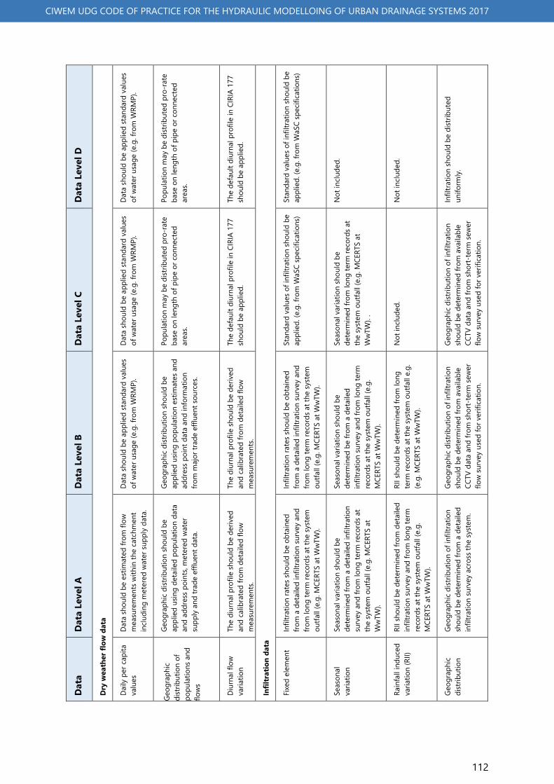
112
CIWEM UDG CODE OF PRACTICE FOR THE HYDRAULIC MODELLOING OF URBAN DRAINAGE SYSTEMS 2017
Dat
a Le
vel D
Dry
wea
ther
flow
dat
a
Data
shou
ld b
e ap
plie
d st
anda
rd v
alue
s of
wat
er u
sage
(e.g
. fro
m W
RMP)
.
Popu
latio
n m
ay b
e di
strib
uted
pro
-rat
e ba
se o
n le
ngth
of p
ipe
or c
onne
cted
ar
eas.
The
defa
ult d
iurn
al p
rofil
e in
CIR
IA 1
77
shou
ld b
e ap
plie
d.
Infil
trat
ion
data
Stan
dard
val
ues o
f inf
iltra
tion
shou
ld b
e ap
plie
d. (e
.g. f
rom
WaS
C sp
ecifi
catio
ns)
Not
incl
uded
.
Not
incl
uded
.
Infil
tratio
n sh
ould
be
dist
ribut
ed
unifo
rmly
.
Dat
a Le
vel C
Data
shou
ld b
e ap
plie
d st
anda
rd v
alue
s of
wat
er u
sage
(e.g
. fro
m W
RMP)
.
Popu
latio
n m
ay b
e di
strib
uted
pro
-rat
e ba
se o
n le
ngth
of p
ipe
or c
onne
cted
ar
eas.
The
defa
ult d
iurn
al p
rofil
e in
CIR
IA 1
77
shou
ld b
e ap
plie
d.
Stan
dard
val
ues o
f inf
iltra
tion
shou
ld b
e ap
plie
d. (e
.g. f
rom
WaS
C sp
ecifi
catio
ns)
Seas
onal
var
iatio
n sh
ould
be
dete
rmin
ed fr
om lo
ng te
rm re
cord
s at
the
syst
em o
utfa
ll (e
.g. M
CERT
S at
W
wTW
). .
Not
incl
uded
.
Geog
raph
ic d
istrib
utio
n of
infil
tratio
n sh
ould
be
dete
rmin
ed fr
om a
vaila
ble
CCTV
dat
a an
d fro
m sh
ort-
term
sew
er
flow
surv
ey u
sed
for v
erifi
catio
n.
Dat
a Le
vel B
Data
shou
ld b
e ap
plie
d st
anda
rd v
alue
s of
wat
er u
sage
(e.g
. fro
m W
RMP)
.
Geog
raph
ic d
istrib
utio
n sh
ould
be
appl
ied
usin
g po
pula
tion
estim
ates
and
ad
dres
s poi
nt d
ata
and
info
rmat
ion
from
maj
or tr
ade
efflu
ent s
ourc
es.
The
diur
nal p
rofil
e sh
ould
be
deriv
ed
and
calib
rate
d fro
m d
etai
led
flow
m
easu
rem
ents
.
Infil
tratio
n ra
tes s
houl
d be
obt
aine
d fro
m a
det
aile
d in
filtra
tion
surv
ey a
nd
from
long
term
reco
rds a
t the
syst
em
outfa
ll (e
.g. M
CERT
S at
Ww
TW).
Seas
onal
var
iatio
n sh
ould
be
dete
rmin
ed b
e fro
m a
det
aile
d in
filtra
tion
surv
ey a
nd fr
om lo
ng te
rm
reco
rds a
t the
syst
em o
utfa
ll (e
.g.
MCE
RTS
at W
wTW
).
RII s
houl
d be
det
erm
ined
from
long
te
rm re
cord
s at t
he sy
stem
out
fall
e.g.
(e
.g. M
CERT
S at
Ww
TW).
Geog
raph
ic d
istrib
utio
n of
infil
tratio
n sh
ould
be
dete
rmin
ed fr
om a
vaila
ble
CCTV
dat
a an
d fro
m sh
ort-
term
sew
er
flow
surv
ey u
sed
for v
erifi
catio
n.
Dat
a Le
vel A
Data
shou
ld b
e es
timat
ed fr
om fl
ow
mea
sure
men
ts w
ithin
the
catc
hmen
t in
clud
ing
met
ered
wat
er su
pply
dat
a.
Geog
raph
ic d
istrib
utio
n sh
ould
be
appl
ied
usin
g de
taile
d po
pula
tion
data
an
d ad
dres
s poi
nts,
met
ered
wat
er
supp
ly a
nd tr
ade
efflu
ent d
ata.
The
diur
nal p
rofil
e sh
ould
be
deriv
ed
and
calib
rate
d fro
m d
etai
led
flow
m
easu
rem
ents
.
Infil
tratio
n ra
tes s
houl
d be
obt
aine
d fro
m a
det
aile
d in
filtra
tion
surv
ey a
nd
from
long
term
reco
rds a
t the
syst
em
outfa
ll (e
.g. M
CERT
S at
Ww
TW).
Seas
onal
var
iatio
n sh
ould
be
dete
rmin
ed fr
om a
det
aile
d in
filtra
tion
surv
ey a
nd fr
om lo
ng te
rm re
cord
s at
the
syst
em o
utfa
ll (e
.g. M
CERT
S at
W
wTW
).
RII s
houl
d be
det
erm
ined
from
det
aile
d in
filtra
tion
surv
ey a
nd fr
om lo
ng te
rm
reco
rds a
t the
syst
em o
utfa
ll (e
.g.
MCE
RTS
at W
wTW
).
Geog
raph
ic d
istrib
utio
n of
infil
tratio
n sh
ould
be
dete
rmin
ed fr
om a
det
aile
d in
filtra
tion
surv
ey a
cros
s the
syst
em.
Dat
a
Daily
per
cap
ita
valu
es
Geog
raph
ic
dist
ribut
ion
of
popu
latio
ns a
nd
flow
s
Diur
nal f
low
va
riatio
n
Fixe
d el
emen
t
Seas
onal
va
riatio
n
Rain
fall
indu
ced
varia
tion
(RII)
Geog
raph
ic
dist
ribut
ion

Page 113 of 169
CIWEM UDG CODE OF PRACTICE FOR THE HYDRAULIC MODELLOING OF URBAN DRAINAGE SYSTEMS 2017
Table C-2 Typical Data Sources for UK Urban Drainage Projects
Category Sub- Category Likely Source (UK)
Sewers – Existing Models Hydraulic models and supporting data WaSC
Sewers – Existing Asset Data
Sewers and manholes WaSC Overflows WaSC Pumping stations WaSC Detention Tanks WaSC Wastewater Treatment Works (WwTWs) WaSC Other ancillaries - pipe bridges, Anti-Flood Devices (AFDs), Inverted Siphons etc. WaSC
Sewers – Existing Survey data
Manhole and asset surveys WaSC Topographical surveys WaSC CCTV Surveys WaSC Sewer flow surveys WaSC Infiltration surveys WaSC Contributing area surveys (CAS) WaSC
Sewers - Live data Live Data: MCERTS, EDM, SCADA, Permanent flow/depth monitors WaSC
Sewers - Operational data Historical wastewater flooding records WaSC Blockages / siltation / tree roots etc. WaSC Sewer collapses / rising main failures WaSC
Sewers - Previous reports and outputs for historical and committed schemes
Previous and committed wastewater solutions data (reports, models, as-constructed drawings, detailed and outline design drawings
WaSC
Sewers - Current and historical reports and outputs for planning studies, flood risk assessment etc.
Previous study outputs – DAPs, SMPs, FRAs, UPMs, etc. WaSC
Tides Tide level data
Tide Tables Harbour Chart Online services National tide gauge network (UK)
Rivers River models River cross sections and control structures River levels and flows – live and historical
Environmental Regulator Flood Authority CEH (FEH)
Geology and Hydrogeology
Geological maps BGS Hydrogeological maps BGS
Borehole data BGS / Site Investigations / Environmental Regulator/ WaSC
Groundwater flooding data BGS, Flood Authority Groundwater models BGS, Environmental Regulator Springs BGS Historic groundwater levels BGS WFD groundwater monitoring points Environmental Regulator
Soils Data Soil data (WRAP/FSR, HOST, University of Cranfield) University of Cranfield, IOH, FSR
DWF and Design Horizon Data: Population, PCC, Trade, MCERTS, Development
Population data WaSC, ONS, Planning Authority Per Capita Consumption (PCC) WaSC MCERT Final Effluent Date WaSC Trade effluent data WaSC Commercial flow data WaSC

114
CIWEM UDG CODE OF PRACTICE FOR THE HYDRAULIC MODELLOING OF URBAN DRAINAGE SYSTEMS 2017
Category Sub- Category Likely Source (UK)
Recent and planned development WaSC
Rainfall and Climate Change
Existing rainfall series WaSC Flood Estimation Handbook (FEH) design rainfall
WASC Existing Models, FEH Website (CEH)
Historical rain gauge and radar data
Environmental Regulator, Meteorological Office
UK Climate Projections 2009 (UKCP09) / Department for Environment Food and Rural Affairs (Defra) guidance
Defra
Environmental Data: Pollution, WFD, Environmental permits, Sensitive areas
Pollution incidents WaSC, Environmental Regulator Environmental permits for discharges (intermittent and continuous) WaSC
River classifications (WFD) Environmental Regulator River status (main river / ordinary watercourse) Environmental Regulator Bathing Water and Shellfish Waters data Environmental Regulator Environmentally sensitive areas [Sites of Special Scientific Interest (SSSI), Special Areas of Conservation (SAC), Special Protection Areas (SPA) and Ramsar, etc.]
Defra
Background mapping and DTM
OS master map Ordnance Survey
LiDAR / Next Map DTM Environmental Regulator, WaSC, Commercial websites
Address points and postcodes WaSC/Ordnance Survey Land use data Ordnance Survey
Flood Risk
Fluvial and pluvial flood maps and historical flood outlines Environmental Regulator, LLFA
Strategic Flood Risk Assessment (SFRA), Local Flood Risk Assessment (LFRA), Surface Water Management Plan (SWMP), Preliminary Flood Risk Assessment (PFRA)
Lead Local Flooding Authority (LLFA) and District Council (DC) Websites
Highways drainage, land drainage and private drainage assets and performance
Highway drainage information Highways Authority, Highways agency
Land drainage information Land Drainage Authority
Railway drainage information Network Rail, London Underground
Internal Drainage Board (IDB) information Flood Authority and IDBs Private drainage and wastewater treatment Private land owners
Canals, Navigable rivers, harbours
Canal information Canal and Rivers Trust (UK) Navigable Rivers information River navigation authorities Harbours and ports information Harbour authorities
Anecdotal data, primary and secondary evidence
Eye witness accounts Public websites (Facebook, newspapers, etc.) Social media accounts

115
CIWEM UDG CODE OF PRACTICE FOR THE HYDRAULIC MODELLOING OF URBAN DRAINAGE SYSTEMS 2017
APPENDIX D - ASSET DATA COLLECTION
Asset record data
Commissioning Bodies generally hold urban drainage asset record data in digital format. However, it may be necessary to obtain other stakeholder data to build the model to an appropriate level of detail. The data are usually available in the form of databases which may be accessed through Geographical Information Systems (GIS). Older records may be held in hard copy formats. Note that these records will rarely be complete.
Asset Surveys
Asset surveys record the main structures which influence the catchment’s flow conditions whether in drainage networks, rivers or at coastal locations. The extent of asset surveys required will largely depend on the confidence requirements linked to the use and purpose of the model. Budget constraints, identified and agreed with the Commissioning Body at the model definition phase of the project will influence the extent of such surveys.
Surveys involving underground structures will require confined space entry in dangerous environments (mechanical equipment, power supplies, dangerous atmospheres, etc.). These assets should only be surveyed where absolutely required and all other alternative sources of information have been investigated and found unsuitable for use. At times it may be appropriate to apply sensitivity testing rather than placing someone in a potentially life threatening environment.
Typically, assets requiring surveys may include, but not be limited to, manholes and key ancillaries such as overflows, bifurcations, dual manholes, pumping stations, detention tanks, outfall structures, inverted siphons and other control structures.
The locations for manhole surveys may also include:
• Flow monitor locations
• Immediately upstream and downstream of ancillaries and flow monitors
• Major junctions
• Low spots
• Areas of known hydraulic deficiencies
• Areas with specific drivers for investigation
The aim of any surveys should be discussed with the survey contractor so that any relevant information can be collected at the same time as the asset survey.
Pipes, channels and manholes
The pipe data needed to build a model is as follows:
• Details of the drainage network and connectivity
• Ground levels
• Dimensions and shape

116
CIWEM UDG CODE OF PRACTICE FOR THE HYDRAULIC MODELLOING OF URBAN DRAINAGE SYSTEMS 2017
• Invert and other key levels
• Material
Typically, most of this data apart from levels will be available from existing urban drainage records. This should be used to define the nodes and links. The pipe material may help in defining the roughness and condition.
Where data are missing, surveys may be required, depending on the location and purpose of the model. . In less detailed models, surveys may sometimes be avoided by making best use of other level data such as mapping spot heights, DTM, or by calculating invert levels from known depths, or by interpolation from levels at adjacent manholes.
This inferred data may sometimes be used in Type I, or in limited cases, Type II models directly, or it may be used to assist in any simplification process adopted, reducing the requirement for surveys. An assessment should be made as to whether the inferred data are critical to the location, or requirements of the study, in which case appropriate surveys should be undertaken.
Manhole surveys should be carried out in accordance with the Commissioning Body standard specification/framework documentation where available. In the UK these are usually based on the “Model Contract Document for Manhole Location Surveys & Production of Record Maps” (WRc, 1993).
The purpose of manhole surveys is twofold. Firstly, to gain an understanding of the quality of the existing commissioning authority asset data and secondly, to enhance the detail of the model for the intended purpose. Focus should remain on what is needed rather than what would be ‘nice to have’ to limit the extents of such surveys. For model enhancement projects the manhole surveys will be targeted at adding additional detail to an existing model but there is still a requirement to check existing data to ensure data sets have the same relative datum.
If a manhole survey is requested, the following information should normally be obtained:
• Full Grid Reference
• Manhole number (Unless already currently referenced in which case that reference will be retained. Where new manhole references are to be given to manholes these will be numbered using the system as instructed by the Commissioning Body)
• Location (OS Plan containing the existing sewer record)
• Function/Use
• Cover level
• All pipe depths to invert
• Upstream/downstream manhole references
• Materials
• Backdrop depth
• All pipe sizes and diameters
• Evidence of surcharge
The survey should include also an assessment and comments on the service condition of pipes (e.g. sediment, encrustation and other internal issues which may influence flows). These

117
CIWEM UDG CODE OF PRACTICE FOR THE HYDRAULIC MODELLOING OF URBAN DRAINAGE SYSTEMS 2017
observations can only hope to pick up issues in the immediate vicinity of manholes. CCTV and or man-entry surveys will be required for a more comprehensive full length survey of the structural and service condition of pipelines.
Rising mains
Data collection requirements for rising mains will depend on the modelling approach in the specific software. However, for most models and the associated reporting, typical information to record or collect can include:
• Diameter
• Length
• Starting asset reference
• Finishing asset reference
• Material
• Locations and sources of connections
Other information required may include valves and other flow control or operational devices (air valves, reflux valves, surge controls). For most drainage models, these will not be implicitly included but their impact may need to be considered as part of any operational verification or calibration, especially when investigating a problem.
Ancillaries
Introduction
Data for ancillary structures, such as combined sewer overflows, bifurcations, on-line and off-storage tanks, control structures and pumping stations, can profoundly affect the results of a sewer model. Ancillary data may already exist and the availability of the following should be checked prior to surveying, including:
• Existing models and accompanying reports
• Historical surveys
• As constructed drawings
• Telemetered operational information
Ancillary structures should normally be identified for a full survey where they have a significant effect on the flow conditions and existing data are of insufficient quality for modelling purposes. It is useful for the modeller to attend complex surveys to ensure that all necessary data are retrieved and to observe any issues that may assist later in the modelling process.
Overflows
Overflows within the study area, or within the influence of a study area, should be surveyed where good quality information is not available from previous surveys or record drawings. The surveys should identify the key hydraulic components and be detailed enough to enable these to be included/represented within the model.

118
CIWEM UDG CODE OF PRACTICE FOR THE HYDRAULIC MODELLOING OF URBAN DRAINAGE SYSTEMS 2017
The following information will generally be measured and recorded, if applicable:
• Chamber dimensions and levels
• Benching details
• Incoming and outgoing pipe dimensions and levels
• Flow control type and dimensions
• Weir length, crest level and width
• Weir orientation (side or transverse)
• For elevated channels with weirs: dimensions of under channel return to spill pipe
• Screen details and dimensions
• Scum board details and dimensions
• Spill pipe and outfall details including flap valves
• Outfall screen details
• Monitoring details (e.g. EDM)
Head discharge relationships for screens and proprietary control devices should be obtained from manufacturers. In some cases a national database is available for these (e.g. Hydro-Brakes).
Pumping Stations
Typically the following information will be required to represent pumping stations in a model:
• Number of pumps
• Pump type
• Pump characteristics
• On/off levels
• Nominal capacity
• Pump curve/head-discharge relationship
• Pump arrangement – duty/standby or duty/assist
• Pump control philosophy (RTC)
• Wet well dimensions
• Rising main details
• Emergency overflow and CSO details
Existing information should be used if available from previous drop tests/surveys, operating manuals and manufactures data. Pump control logic and current operating regimes should be understood and operations staff should be consulted together with the collection of any available design documentation that will assist in representing the pumping station in the model. Any monitoring data available should also be collected (such as pump run time logs, depth data, etc.).

119
CIWEM UDG CODE OF PRACTICE FOR THE HYDRAULIC MODELLOING OF URBAN DRAINAGE SYSTEMS 2017
Depending on the configuration of the station, Real Time Control (RTC) may be required to control pump start and stop and/or pump rates. Understand the current operating conditions to avoid lengthy verification using incorrect/out of date conditions.
Pump capacities are normally determined by carrying out a “drop test”. This involves measuring the plan area of the wet well and then measuring the change in water level for a cycle of the pump running and stopped. It assumes the inflow to the wet well remains constant over the cycle and calculates the pump capacity from the difference between the rise rate and fall rate of the water level. This process should be repeated for each pump individually and for each combination of pumps that may operate together.
There are several precautions that are required to ensure that accurate results are achieved. These include:
• Any pumping stations upstream that could cause rapid changes in the inflow rate should be switched off for the duration of the test
• The test should be carried out over a large enough depth range so that the measurements are accurate
• The test should be carried out at least three times to ensure repeatable results
• The depth range should not include low depths where the pump casing or the benching reduce the cross sectional area, nor high depths where the incoming pipes increase the area
• Pump combinations that do not operate should not be tested and reported. This is a particular concern where duty and standby pumps are both run together with the potential to damage the rising main. It is also a significant cause of confusion in modelling correct operation
• Results should be sanity checked so that notionally similar pumps should give similar capacities and two pumps always give more flow than one pump
Due to some uncertainties over pump tests, if not undertaken or interpreted correctly, an alternative is to back calculate from depth monitor results. However, there are benefits to carrying out drop tests:
• They accurately relate capacities to pump combinations without requiring run time monitors
• They allow the pumps to be modelled correctly before the flow survey is carried out
• They can identify pump faults that could be remedied before the flow survey is carried out, so giving better survey results
Where the rising mains combine with flows with other pumping stations, then this will require a different testing regime due to the potential different pumping heads. Ideally, multiple pumps and combinations should be tested running simultaneously.
Other Ancillaries
Other hydraulically significant ancillaries with missing data should be identified for a survey, where key data are not available from other sources or is of insufficient quality, including. These may include:

120
CIWEM UDG CODE OF PRACTICE FOR THE HYDRAULIC MODELLOING OF URBAN DRAINAGE SYSTEMS 2017
• Detention Tanks (including upstream and downstream manholes)
• Inverted Siphons (including upstream and downstream manholes);
• Outfall structures including screen and flap valves
• Other significant ancillaries affecting hydraulic performance
WwTW
There are many components in a WwTW that may require representation in a hydraulic model. It is common practice to represent the WwTW as far as the FFT control. In cases more detail may be added to represent downstream processes; in other cases less detail is needed, and the requirement is merely to represent the boundary condition created by the WwTW. Typically, the following components may be represented explicitly necessitating the collection of specific data:
• Inlet (6DWF) and Storm Tank Overflows (3DWF)
• Inlet Screens
• Works Pumping Stations
• Flow channels
• Flow controls
• Online storage
• Offline storage - Storm Tanks including overflow and storm return
• Outfall channels pipes including flap valves
• FFT
• Operating manuals and control rules for FFT, pumping stations, storm tank returns, etc.
It is recommended that a site visit is undertaken if the WwTW is to be included in the model. Inlet arrangements at WwTWs can vary widely and hydraulic controls/influences cannot always be seen from record drawings. Site visits are essential to understand individual hydraulic structures/controls and any interactions between them. It is important to obtain as much information from site operatives as possible to fully understand current operating regimes and such information should be recorded and documented clearly. Collection of as built information may be required to determine the extents of survey requirements to check the quality of as built information and ensure any modifications are captured and included in the model.
Where surveys are required, overflows and pumps within the WwTW should be surveyed the same as the catchment’s other CSOs and PSs where site constraints allow.
Other data requirements include the WwTW permit information, inflow data (e.g. MCERTS (UK)), EDM spill data and other monitoring data which should be obtained for the full period of record where available. Care should be taken to ensure that the correct units for any flows are reported as well as their monitoring locations. For example, FTFT can be reported downstream of the storm tanks and include elements of storm return flows. Consideration may need to be given to the wastewater treatment biological process to ensure that there are no unexpected impacts on the hydraulic representation.

121
CIWEM UDG CODE OF PRACTICE FOR THE HYDRAULIC MODELLOING OF URBAN DRAINAGE SYSTEMS 2017
Real Time Control (RTC)
Control philosophies and logic for complex pumping stations, controlled overflows etc.; should be downloaded from control panels and analysed where possible for inclusion in the model. If this is not possible, the RTC rules may be obtained from O&M manuals, existing models and/or estimated by reviewing records of flows from long or short-term flow data. This data should be supported by detailed discussions with operational staff to understand how the controls operate in extreme events
Sustainable drainage systems
A detailed site walkover should be carried out where SUDS require modelling to assess their operational condition. Key issues to consider include outfall/overflow condition, level of maintenance and siltation levels. Data requirements for SUDS essentially follow the same principles as for other ancillaries, but the data may be harder to determine or establish. The aim of the model is to represent the features hydraulic performance. This can be done as part of an explicit representation of flow paths and in some instances it may be appropriate to represent their impact by other modelling approaches. The representation of SUDs and data collection should consider the following components:
• Source control – area affected and exceedance needs, runoff factors
• Infiltration – area and ground conditions
• Conveyance – channel dimensions, vegetation types
• Storage – dimensions, soil, lining, flow controls, exceedance routes
Depending on the complexity of the modelling software and approach being applied, a more detailed list of data that could be collected is summarised in Table D-1.
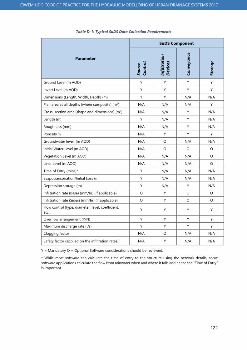
122
CIWEM UDG CODE OF PRACTICE FOR THE HYDRAULIC MODELLOING OF URBAN DRAINAGE SYSTEMS 2017
Table D-1: Typical SuDS Data Collection Requirements
Parameter
SuDS Component
Sour
ce
Cont
rol
Infil
trat
ion
Dev
ices
Conv
eyan
ce
Stor
age
Ground Level (m AOD) Y Y Y Y
Invert Level (m AOD) Y Y Y Y
Dimensions (Length, Width, Depth) (m) Y Y N/A N/A
Plan area at all depths (where composite) (m2) N/A N/A N/A Y
Cross section area (shape and dimensions) (m2) N/A N/A Y N/A
Length (m) Y N/A Y N/A
Roughness (mm) N/A N/A Y N/A
Porosity % N/A Y Y Y
Groundwater level (m AOD) N/A O N/A N/A
Initial Water Level (m AOD) N/A O O O
Vegetation Level (m AOD) N/A N/A N/A O
Liner Level (m AOD) N/A N/A N/A O
Time of Entry (mins)* Y N/A N/A N/A
Evapotranspiration/Initial Loss (m) Y N/A N/A N/A
Depression storage (m) Y N/A Y N/A
Infiltration rate (Base) (mm/hr) (if applicable) O Y O O
Infiltration rate (Sides) (mm/hr) (if applicable) O Y O O
Flow control (type, diameter, level, coefficient, etc.). Y Y Y Y
Overflow arrangement (Y/N) Y Y Y Y
Maximum discharge rate (l/s) Y Y Y Y
Clogging factor N/A O N/A N/A
Safety factor (applied on the infiltration rates) N/A Y N/A N/A
Y = Mandatory O = Optional Software considerations should be reviewed.
* While most software can calculate the time of entry to the structure using the network details, some software applications calculate the flow from rainwater when and where it falls and hence the “Time of Entry” is important.

123
CIWEM UDG CODE OF PRACTICE FOR THE HYDRAULIC MODELLOING OF URBAN DRAINAGE SYSTEMS 2017
Watercourses and open channels
Watercourses should be considered in similar way to any other part of the urban drainage system where included in an urban drainage model. The following data requirements will apply where watercourses are modelled:
• River cross-sections should be taken at all significant changes in channel form, and in most urban contexts at least every 100m. Data requirements will be sections (x, y and z) with banks defined looking downstream
• Details of river control structures such as bridges and weirs will be required where they could be expected to impact the model results within the scenarios the model is designed to represent
Open channels are classified by the flow having a free surface and are sub-divided into two groups:
• Natural Channel (Irregular Shape)
• Artificial Channel (Regular Shape)
Cross section and control structure data for rivers may be obtained from existing river models or historic survey data where available. Where Open channel or river control structure surveys are required the EA (2013) National Standard Contract and Specification for Surveying Services and the CIWEM UDG (1999) River Data Collection Guide provides further guidance.
Particular care is required when considering exceedance flows and extreme events to ensure that all flow routes are represented. It should be noted that a flood risk model may contain many more structures than a model solely looking at water quality.
System Connectivity
Where the connectivity of urban drainage systems is uncertain from asset records then further investigations on site may be undertaken to gather the required information. Methods of connectivity testing include:
• Sound testing
• Dye Tracing
• Smoke testing
• CCTV survey
Real time controls (RTC)
It can be difficult to understand the operating rules for complex pumping stations, overflows, storage tanks and other ancillaries merely by observing or surveying their operation. It is therefore important to obtain control philosophies and operating manuals for these and to understand that they may not be operated as designed. It is often beneficial to obtain a download of the operating logic from the control device so that this can be analysed to understand the real operation. This task should always be undertaken with the system operator’s approval and carried out by instrumentation specialists, as there is a risk of disrupting the operation of the controls when downloading the control logic. Site operatives

124
CIWEM UDG CODE OF PRACTICE FOR THE HYDRAULIC MODELLOING OF URBAN DRAINAGE SYSTEMS 2017
should be consulted where ancillaries are suspected to be operating outside their control rules. In some cases this may be due to manual interventions.
Non Man Entry Surveys
In addition to physical attributes, the operational and structural condition of urban drainage systems are very important factors that can be the main cause of issues such as flooding in a catchment. The condition of the pipes, for example, can have a significant impact on the pipe roughness and sediments may reduce the cross-sectional area of the pipes and increase roughness.
To better understand the condition of the pipes in a catchment the existing CCTV surveys should be collected from the commissioning authority if available. Depending on the age/availability of such information it may be necessary to undertake further CCTV surveys for the study. This should be planned an undertaken in line the commissioning authority’s own specification or where this is not available, the Model Contract Document for Sewer Condition Inspection (WRc, 2005).
Contributing Areas Surveys (CAS)
Contributing area surveys (CAS) involve the survey of roofs, roads and other paved surfaces, and in some cases permeable surfaces in order to:
• Establish the general patterns of drainage within the survey area
• Quantify and qualify the different types of runoff areas within the survey area
• Establish the connectivity of the runoff areas to the urban drainage system(s)
This type of survey usually depends on the Commissioning Body’s requirements and budgetary constraints. Specific development types should therefore be targeted (partially separate systems, separate systems, large industrial areas or commercial developments) where records are not available or storm contribution is uncertain and could influence the model’s performance. The results of the CAS will assist in the calibration of runoff in areas where the degree of separation between foul and surface water is unclear and so provide some level of validation to the parameters included in the model. In some cases, it may be necessary to undertake further surveys where the model cannot replicate measured flows.
The sampling rate for CAS will vary depending on the age and type of development but in general the overall property sampling rate is typically in the range 10 - 15 %. However, in urban or sub-urban areas where properties are of a similar age and design, the sampling rate may be reduced to as low as 5%...Conversely in areas where there exists a wide variation in the age and/or design of properties, an increased the sampling rate may be required especially in established rural catchments. Where there is an intention to undertake surface water disconnections from combined systems, it may be necessary to target even more properties, although this may be undertaken at a later stage.
Contributing area surveys are particularly useful where there are either small pipe sizes (<225mm) or very steep pipes that create hydraulic conditions unsuitable for conventional flow monitoring. In particular, this may include separate or partially separate systems.

125
CIWEM UDG CODE OF PRACTICE FOR THE HYDRAULIC MODELLOING OF URBAN DRAINAGE SYSTEMS 2017
CAS results should ideally be created in a GIS format to enable all the survey findings to be imported directly into the preferred modelling software. A suitable colour coding system for GIS output showing the means of surface water disposal is also beneficial in visualising the data. Table D-2 presents example colours and application.
Table D-2 Possible colours for CAS output
Surface Water Disposal Method
GIS Display Colours for Flow Sources Pitched Roof Paved Areas and Flat Roofs
Soakaway and permeable areas Yellow Yellow Foul/combined sewers Red Brown Surface water sewers Blue Green Direct to road or pavement Mauve N/a

Page 126 of 169
APPENDIX E - Runoff Models
This note summarises the following rainfall-runoff models including their characteristics, calibration and use in urban drainage modelling.
• Fixed percentage runoff
• Wallingford Procedure (Fixed) - Old PR model
• New UK (Variable) - New PR model
• UKWIR Runoff Model
Rural / Pervious runoff models
Each of the following models is described in more detail in the Literature Review and Guide for the UKWIR Project: Development of the UKWIR Runoff Model (UKWIR (2014).
• Green-Ampt
• Horton
• Flood Estimation Handbook Revitalised rainfall runoff (ReFH/ReFH2) Model
• Probability Distributed Model (PDM)
• USA Soil Conservation Service (SCS) method
Table E–1 summarises the key attributes of each model.
Table E–1 Runoff models and their characteristics
Runoff Model Application Comments
Fixed percentage runoff
Primarily Impervious areas but may applied to pervious areas
Mainly used for impervious surface runoff only. Typical parameter values well understood in the UK. Percentage runoff values are generally not varied between storms or during a storm. Not suited to continuous simulation series or long storm durations
Wallingford Procedure (Fixed) – Old PR model
Impervious and pervious surfaces in an urban setting
Correlation equation based on soil type, wetness and proportion of paved surface. Superseded by New PR equation, but still in use in some models. Parameter values easily measured and well understood in the UK. Percentage runoff does not vary during each storm so not suited to long storm durations. Theoretically can be used for continuous simulation as wetness can be updated for the start of each event.
New UK (Variable) - New PR model
Impervious and pervious surfaces in an urban setting
Suited to impervious and pervious surface modelling. Typical parameter values well understood in the UK. Percentage runoff varies over time through the storm
UKWIR runoff model
Impervious and pervious surfaces in an urban setting
Developed to address perceived limitation of New UK runoff model Suited to impervious and pervious surface modelling The paved runoff has a wetting effect to increase runoff with rainfall depth;

127
CIWEM UDG CODE OF PRACTICE FOR THE HYDRAULIC MODELLOING OF URBAN DRAINAGE SYSTEMS 2017
Runoff Model Application Comments Paved areas which are not directly served with drainage can be treated as different paved surface types with their own runoff characteristics; Includes the facility to use HOST categorisation of soils as well as WRAP soil classes; Facilitates the ability to meet the differences in runoff between winter and summer conditions; Pervious runoff has been shown to not exceed rural runoff predictions from ReFH – therefore addressing concerns of over-prediction of runoff volume.
Green-Ampt infiltration model
Pervious surfaces (esp 2D)
Physically based model. Intended for modelling runoff from pervious surfaces. Parameter selection relies on knowledge of physical soil properties Percentage runoff varies over time through the storm Soil drying represented to allow continuous simulation Does not include evapotranspiration
Horton infiltration model
Pervious surfaces (esp 2D)
See comments Green-Ampt above.
Flood Estimation Handbook Revitalised rainfall runoff model (ReFH)
Rural catchments hydrology
Extreme events runoff Part of hydrological model for flooding in rural catchments Parameters can make use of readily available Flood Estimation Handbook catchment descriptors Designed for rural rivers rather than small pervious catchments in the urban environment
Probability Distributed Model (PDM)
Extreme events runoff Part of hydrological model for flooding in rural catchments Parameters require calibration from observed data Designed for rural rivers rather than small pervious catchments in the urban environment
USA Soil Conservation Service method (SCS)
Pervious surfaces – normally rural catchments
Designed for modelling runoff from pervious surfaces and rural catchments Commonly applied outside UK (mainly US). Parameter selection relies on land use classification to select curve number Percentage runoff varies over time through

128
CIWEM UDG CODE OF PRACTICE FOR THE HYDRAULIC MODELLOING OF URBAN DRAINAGE SYSTEMS 2017
APPENDIX F - SCATTERGRAPHS
The recorded flow data for each monitor should be reviewed by plotting scattergraphs. This may be done for different storm events or different interim data periods using different colours. The scattergraphs should also show the Colebrook-White line for the pipe in which the monitor was installed.
Where a flow monitor is installed in an incoming pipe into a manhole it is useful to add the Colebrook-White line for the outgoing pipe also. It is possible that the outgoing pipe is governing the flow conditions at that flow monitor.
Ideally the scattergraph should be plotted to a log-log scale and can either be flow/depth or velocity/depth. The illustrations shown later are for flow/depth plots and these help the quality of flow survey data to be assessed. Interpretation of velocity/depth scattergraphs is more difficult but can be a useful means of understanding the flow conditions during the flow survey. Velocity/depth scattergraphs may only be needed where a greater understanding is required to adequately classify the quality of the flow survey data.
Scattergraphs for dry weather periods can often be affected by the monitoring equipment interfering with or partially obstructing the flow, especially where the flows are shallow. It is recommended that dry weather scattergraphs are only plotted and assessed at a selection of the monitoring sites where the flows are sufficient to enable meaningful assessment.
The data should be classified by means of a visual observation of the consistency of the data and the closeness of the fit to the Colebrook-White line. This can use a subjective classification of as “very good”, “good”, “fair” or “poor”. The interpretation and classification of the scattergraphs should consider if there are inaccuracies in data used to calculate the flows and depths. For example, a departure from the Colebrook-White line may indicate that the invert levels, pipe gradient or pipe size might be incorrect in the model, there may be sediment in the downstream pipes or the system has a downstream control causing for example an increase in depth.
Examples of scattergraphs plotted for storm conditions are shown below. An example of a scattergraph is shown in Figure F.1 and the flow survey data for this monitor (M140) has been classified as ‘Very Good’. Further examples of scattergraphs are given in Figure F.2 (good data), Figure F.3 (fair data) and Figure F.4 (poor data).
Verification of a flow monitor should only use data considered to be ‘very good’ or ‘good. Depth data from sites classed as ‘fair’ may still be used as depth data are typically more reliable than flow or velocity. ‘Poor’ data should not normally be used for model verification.
The scattergraph for Figure F.5 is an example of a flow monitor installed a short distance upstream of a CSO. Initially, this may be classified as ‘poor’. However, further examination reveals the data are very good. It departs from the Colebrook-White line when the flow is backed up by the flow control at the CSO (depth increases with no increase in flow) until such time as the water level reaches the overflow weir. At this point there is an increase in flow rate with very little increase in depth then finally a second curvilinear relationship is noted which is governed by the capacity of the CSO spill pipe. In this example the data would be classified as ‘very good’.

129
CIWEM UDG CODE OF PRACTICE FOR THE HYDRAULIC MODELLOING OF URBAN DRAINAGE SYSTEMS 2017
Figure F.2: Example scattergraph for “good” measured flow depth relationship
Figure F.1: Example scattergraph for very good measured flow depth relationship

130
CIWEM UDG CODE OF PRACTICE FOR THE HYDRAULIC MODELLOING OF URBAN DRAINAGE SYSTEMS 2017
Figure F.3: Example scattergraph for “fair” measured flow depth relationship
Figure F.4: Example scattergraph for “poor” flow depth relationship

131
CIWEM UDG CODE OF PRACTICE FOR THE HYDRAULIC MODELLOING OF URBAN DRAINAGE SYSTEMS 2017
Figure F.5 Example Scattergraph where analysis of the relationships between flow and depth in the local context is important to understand its quality
normal flow
normal flow
flow controlled by throttle at d/s CSO
flow over weir
s

132
CIWEM UDG CODE OF PRACTICE FOR THE HYDRAULIC MODELLOING OF URBAN DRAINAGE SYSTEMS 2017
APPENDIX G – EXAMPLE OF STATISITICAL METHOD FOR STORM VERIFICATION: THE NASH-SUTCLIFFE EFFICIENCY COEFFICIENT
The Nash Sutcliffe Efficiency Coefficient (NSEC) formula shown below is a normalised statistic used to assess how well two graphs (observed and predicted) match one another:
NSEC = 1 −Σt=1 T �Qo
t − Qpt �2
Σt=1T �Qot − Q�o �2
Where Qo is observed discharge and Qp is predicted discharge.
When using the statistical approach it should be applied to graphs for flow and depth separately. The formula calculates residual variance by comparing model predicted data with observed data at every available time-step. It provides an assessment of the closeness of the match between peak values and the closeness of the fit in respect of shape and timing.
The overall NSEC score can range between +1 and negative infinity, with a perfect match between predicted and observed data returning a score of 1. Research by Moriasi et al. (2007) states that a NSEC score of 0.5 is a ‘satisfactory’ replication of observed data.
NESC criteria and scores should be set by Commissioning Bodies. The scores should be calculated for depth and flow at each monitor.
For depth, NSEC should be applied where water depth is greater than 10% of the pipe height or 100mm whichever is the greater. This accounts for a simulation programme that may artificially add flow to dry pipes for stability and monitors may not accurately record levels below this threshold.

133
CIWEM UDG CODE OF PRACTICE FOR THE HYDRAULIC MODELLOING OF URBAN DRAINAGE SYSTEMS 2017
APPENDIX H – EXAMPLE APPROACH TO DRY WEATHER VERIFICATION
This appendix sets out a procedure for dry weather verification.
Weekday and weekend dry weather profiles whilst different do not capture the variations observed. This procedure uses all or a large number of dry days within the survey period. All DWF day hydrographs should be combined to create maximum and minimum boundary hydrographs, so creating a window of acceptability. This should be completed for weekday and weekend. Dry days can be defined as a day of zero rainfall that follows a day of less than 1mm of rain. Dry weather verification should be considered ‘good’ if the predicted hydrograph lies between the boundaries.
In some instances where the flow survey data are over a long period and there has been a significant change in baseflow infiltration it may be necessary to remove the baseflow element prior to plotting the DWF day hydrographs.
A simplified version of this approach is shown in Figure H.1. At each time-step, the plotted maximum (in red) and minimum (in blue) values create boundary hydrographs.
A more advanced approach involves smoothing the lines to give more defined boundaries. This helps spiky hydrographs or those which are heavily influenced by upstream or downstream pumping stations as the pump cycles tend to be dampened out. An example of a smoothing method for this is the Savitzky-Golay filter which is shown below.
𝑌𝑌𝑗𝑗 = � 𝐶𝐶𝑖𝑖𝑦𝑦𝑖𝑖+1
𝑖𝑖=(𝑚𝑚−1)÷2
𝑖𝑖=1(𝑚𝑚−1)÷2
𝑚𝑚 + 12
≤ 𝑗𝑗 ≤ 𝑛𝑛 −𝑚𝑚 − 1
2
Where: x is an independent variable,
yj is an observed variable and
m and Ci relate to “convolution coefficients.
The Savitzky-Golay filter works in a similar way to a moving average, but uses ‘convolution coefficients’ and low-degree polynomials. It retains the exact peak and trough times and does not distort the shape of the data. For the values to be generated it uses data from outside of the 24-hour period of the individual dry day. At maximum, 42 minutes of data (at 2-minute intervals) from each of the two adjoining days need to be used.
Figure H.2 shows the Savitzky-Golay filter in use. The base data are the same as for Figure H.1, but the Savitzky-Golay filter smoothes the underlying five DWF days used with the minimum and maximum lines taken from these smoothed lines. Individual dry days which exhibit unusual characteristics (e.g. high depth and low flows due to pump failure downstream) should not be used and removed.
When using long time-series or extended data, only dry days should be used where the recession from preceding storms has fully receded. This for example may be 36 to 48 hours after rainfall has ceased.

134
CIWEM UDG CODE OF PRACTICE FOR THE HYDRAULIC MODELLOING OF URBAN DRAINAGE SYSTEMS 2017
Figure H.1 - Maximum and Minimum Boundary Hydrographs
Figure H.2 - Smoothed Maximum and Minimum Boundary Hydrographs using Savitzky-Golay Filtering

135
CIWEM UDG CODE OF PRACTICE FOR THE HYDRAULIC MODELLOING OF URBAN DRAINAGE SYSTEMS 2017
Figure H.3 - Example of Dry Weather Verification Plots with NSEC and Confidence scores

136
CIWEM UDG CODE OF PRACTICE FOR THE HYDRAULIC MODELLOING OF URBAN DRAINAGE SYSTEMS 2017
APPENDIX I – EXAMPLE OF APPLYING THE NASH-SUTCLIFFE EFFICIENCY COEFFICIENT FOR STORM VERIFICATION
The application of the NESC is shown in Figure I-1. There is a good match in the first peak but an over prediction in the second peak. This causes the NSEC values to drop. These values are above 0.5 and indicate an acceptable verification. Further investigation of the under predicted peaks might be considered to improve the overall NSEC values.
Figure I-1 Depth and Flow Hydrographs (observed in green, predicted in red) with calculated NSEC scores
Figure I-2 shows an example of the storm verification for a flow monitor FM015 for 3 storms. The plots are for depth and flow. The dashed red horizontal line in the depth plots represents 10% of the conduit height and the depth remained above this level throughout the storms.
It contains a summary of key values (see Table 5-1) and the NSEC values beneath each pair of hydrographs.
The filtering system used for the recorded dry day data should not be used for the storm data as the comparison needs to be against the recorded data for that storm event as opposed to a ‘typical’ dry day.
NSEC = 0.78
NSEC = 0.65

137
CIWEM UDG CODE OF PRACTICE FOR THE HYDRAULIC MODELLOING OF URBAN DRAINAGE SYSTEMS 2017
Figure I-2 - Storm Verification Plots with NSEC scores

138
CIWEM UDG CODE OF PRACTICE FOR THE HYDRAULIC MODELLOING OF URBAN DRAINAGE SYSTEMS 2017
APPENDIX J – EXAMPLE OF QUALITATIVE SCORING APPROACH
This appendix contains an example of how a qualitative (R-A-G) scoring approach can be applied. This is not intended to be a definitive scoring system but serves to illustrate how such a system might be developed. This example is for the storm verification of a partially separate catchment which has a mixture of foul, combined and storm sewers. For simplicity foul and combined sewers are treated as being the same.
Verification Assessment Spreadsheet
The storm verification targets as set out in Table 5.1 are used in this scoring system. The assessment is set up in a simple spreadsheet where the observed and simulated data for each of the 3 verification storms are entered. If the match between the observed and the simulated is within the target criteria the cell is coloured green, if it is marginally outside it is coloured amber and if it is further outside it is coloured red.
On the left hand side of the spreadsheet the assessment of the scattergraph quality (poor, reasonable, good or very good) is included and colour coded.
The full spreadsheet is shown in Figure J-4 to illustrate the 4 different sections of the spreadsheet (shape, peak flow, volume and depth) each section is discussed separately below. Separate assessments are done for each storm and then the results in each section are then averaged to give an overall indication.
The following images illustrate the different sections of the spreadsheet.
This section of the spreadsheet (Figure J-1) deals with how well the shapes of the hydrographs match. This is primarily based on the flow hydrograph but the depth hydrograph can be used when there is extensive ragging or poor velocity measurement.
For each of the 3 storms the degree of match has been assessed using the Nash Sutcliffe Efficiency Coefficient (NSEC) which has a range of +1 to -∞. A score higher than 0.5 is considered good and has been colour coded in green, between 0.4 and 0.5 is coloured in amber and lower than 0.4 is coloured red. The average values are coloured in the same way.
Figure J-1 - Example of confidence assessment for hydrograph shape match

139
CIWEM UDG CODE OF PRACTICE FOR THE HYDRAULIC MODELLOING OF URBAN DRAINAGE SYSTEMS 2017
The next section of the spreadsheet (Figure J-2) is for the comparison of peak flows with the observed data shown in black and the simulated values shown in blue. For each storm the values are compared and then on the right hand side the comparison values are averaged.
Where no comparison is made (in this example for any sites with a ‘reasonable’ or ‘poor’ scattergraph assessment) the cells are left blank.
The colour coding used is: +25% to -10%: green +30% to -15%: amber >30% or <-15%: red.
The next section of the spreadsheet is for the comparison of volumes with the observed data again shown in black and the simulated values shown in blue. For each storm the values are compared and then on the right hand side the comparison values are averaged.
As with the peak flows where no comparison is made (in this example for any sites with a ‘reasonable’ or ‘poor’ scattergraph assessment) the cells are left blank.
The colour coding used is: +20% to -10%: green +25% to -15%: amber >25% or <-15%: red.
Figure J-2 - Example of confidence assessment for peak flow
Figure J-2 - Example of confidence assessment for volume

140
CIWEM UDG CODE OF PRACTICE FOR THE HYDRAULIC MODELLOING OF URBAN DRAINAGE SYSTEMS 2017
In Figure J-3 the peak depths are compared. For simplicity in this example the depths are treated the same irrespective of whether the sewer was surcharged or not and were also not considered as ‘critical locations’. In practice it is likely that greater account will need to be taken of whether the sewer was surcharged or not and whether the monitor was at a ‘critical location’.
Those monitors (in this case FM16 & FM17) with a scattergraph assessment of ‘Poor’ are not used for any verification assessments whereas those assessed as ‘Reasonable’ are assessed for peak depth only; this is why in this image there are only two lines with no data.
The colour coding used is: • +0.5m to -0.1m : green
• +0.75m to -0.35m : amber
• >0.75m or <-0.35m: red.
Figure J-4 shows the whole spreadsheet. At the right hand end of the spreadsheet (in this case at the top of the image) is a column for an overall assessment to be made. This is a largely subjective judgement but it is reasonably transparent how it has been arrived at by means of looking across the rows in the spreadsheet.
There are only 3 categories given:
• Good : green
• Reasonable : amber
• Poor : red
These final assessment can then be visualised within the modelling program by means of giving all of the subcatchments upstream of each monitor that assessment. Figure J-5 shows the foul & combined system with the subcatchments colour coded to reflect the confidence assessment and Figure J-6 the shows similar for storm system. Care should be taken with this approach as verification is at a point and a case can be made that confidence will reduce with the distance from the monitoring point.
It is particularly clear in the visualisation for the storm system that large parts of the catchments could not be assigned a confidence because there were no flow monitors installed covering those areas.
Figure J-3 - Example of confidence assessment for peak depth

141
CIWEM UDG CODE OF PRACTICE FOR THE HYDRAULIC MODELLOING OF URBAN DRAINAGE SYSTEMS 2017
Figure J-4 Example of a confidence assessment sheet for storm verification

142
CIWEM UDG CODE OF PRACTICE FOR THE HYDRAULIC MODELLOING OF URBAN DRAINAGE SYSTEMS 2017
Figure J-5 Storm Verification Visualisation for Foul & Combined System
Figure J-6 Storm Verification Visualisation for Storm System

143
CIWEM UDG CODE OF PRACTICE FOR THE HYDRAULIC MODELLOING OF URBAN DRAINAGE SYSTEMS 2017
APPENDIX K – EXAMPLE OF NUMERICAL SCORING APPROACH
This appendix contains an example of how a numerical scoring approach can be applied. This is not intended to be a definitive scoring system but serves to illustrate how such a system might be developed. Values used in the examples for scores and weightings are therefore only included for illustration purposes and are by no means recommendations.
This example is for a conduit and a similar approach can be taken for all aspects.
Scoring Data Flags
The first aspect is to decide on a scoring system for the data flags used in the modelling. This scoring system would need to be applied throughout the model and for all aspects. A score should be determined for data flags that might be used and it is therefore simpler if the number of data flags used is kept to a minimum. Difficulties will arise if modellers are permitted to introduce additional data flags.
Table K-1 gives an example of the data flags that follow an alphanumerical approach with the letter denoting the method of collection and the number denoting a quality assessment.
Table K-1 Example of data flags and scoring
The # data flags that exist in some modelling programs are also scored and it is notable that the #D flag is scored at zero, which is intended to encourage modellers to make a conscious decision about all the data used in the model. Scores for #A, #I and #V are relatively high as they are likely to be used for data imported from GIS data or previous models.
Name Display Colour Description Score
#A Asset Data 7 #D System Default 0 #G Data from GeoPlan 1 #I Model Import 6 #S System Calculated 1 #V CSV Import 6 A1 A1 Quality 10 A2 A2 Quality 9 A3 A3 Quality 8 B1 B1 Quality 8 B2 B2 Quality 7 B3 B3 Quality 6 C1 C1 Quality 7 C2 C2 Quality 6 C3 C3 Quality 5 D1 D1 Quality 6 D2 D2 Quality 5 D3 D3 Quality 4

144
CIWEM UDG CODE OF PRACTICE FOR THE HYDRAULIC MODELLOING OF URBAN DRAINAGE SYSTEMS 2017
The example in Figure K-1 shows how the data flags might appear for a pipe conduit.
Figure K-1 Example of data flags for a pipe conduit
Weightings
Each aspect of the model (Asset data, Subcatchment data etc) will need to have a set of weightings applied, which are based on the relative importance of each item of data to the overall confidence which can be attributed to that asset or subcatchment. The example in Table K-1 gives an illustration of the weightings that might be applied to a conduit in the model.
It will be necessary for the personnel developing the scoring system to have a detailed understanding of hydraulics and how the modelling program utilises the data, in order that appropriate weightings can be determined.
If the scoring system is based upon a series of SQL’s which can be embedded in the model it will be necessary for the weightings for each aspect of asset data etc to be hard coded into the SQL.

145
CIWEM UDG CODE OF PRACTICE FOR THE HYDRAULIC MODELLOING OF URBAN DRAINAGE SYSTEMS 2017
Table K-1 Example of weightings for links
Example for Circular Pipe
The percentage score for this pipe is based on comparing the actual score with the maximum attainable score, assuming the maximum score can be achieved for every item. In this example the percentage score is 80.6% which signifies a high degree of confidence (Table K-2).
This example is presented in a spreadsheet format and whilst a quantitative scoring system could utilise a spreadsheet or database it is more likely to be developed as a series of SQL’s which automatically calculate the total score and add the answer to a ‘User Number’ field. In this way the confidence can be displayed within the geoplan view (Figure K-2) of the modelling program as illustrated below.
In this example both the pipe size and the quantitative score are displayed for each pipe in the network. The pipes are also colour coded according to their quantitative score banding. The foul and combined sewers are shown as the solid lines and the storm sewers are shown as dashed lines.
Link Definition Weighting US Node ID 10 DS Node ID 10 Link Suffix 3 Link Type 10 Asset ID - Sewer Reference - System Type 5 Branch ID - Conduit Definition Weighting Solution model 5 Minimum computational nodes 5 Critical sewer category - Taking off reference - Conduit material 4 Design Group - Site Condition - Ground condition - Cross section Weighting Shape ID 10 Width (mm) 9 Height (mm) 9* Sediment depth (mm) 8
∗ In some programs data flags cannot be assigned to the Height when the shape is circular
Roughness parameters Weighting Roughness type 7 Bottom roughness 7 Top roughness 7 Long Section Weighting Length (m) 8 Inflow (m3/s) 10 Gradient (m/m) - Full capacity (m3/s) - US invert level (m AD) 10 DS invert level (m AD) 10 US headloss type 6 DS headloss type 6 US headloss coefficient 2 DS headloss coefficient 2

146
CIWEM UDG CODE OF PRACTICE FOR THE HYDRAULIC MODELLOING OF URBAN DRAINAGE SYSTEMS 2017
Table K-2 Example of calculating the confidence score for a pipe
Link Definition Weighting
Data Flag
Data Flag Score
Weighted Score
US Node ID 10 A2 9 90 DS Node ID 10 B2 7 Link Suffix 3 A2 9 27 Link Type 10 A1 10 100 Asset ID - Sewer Reference - System Type 5 B2 7 35 Branch ID - Conduit Definition Solution model 5 #A 7 35 Minimum computational nodes 5 A1 10 50 Critical sewer category - Taking off reference - Conduit material 4 B2 7 28 Design Group - Site Condition - #D 0 Ground condition - #D 0 Cross section Shape ID 10 #A 7 70 Width (mm) 9 A2 9 81 Height (mm) 9* A2 9 Sediment depth (mm) 8 B2 7 56 Roughness parameters Roughness type 7 A1 10 70 Bottom roughness 7 B2 7 49 Top roughness 7 B3 6 42 Long Section Length (m) 8 #A 7 56 Inflow (m3/s) 10 B1 8 80 Gradient (m/m) - Full capacity (m3/s) - US invert level (m AD) 10 A2 9 90 DS invert level (m AD) 10 B2 7 70 US headloss type 6 B1 8 48 DS headloss type 6 B1 8 48 US headloss coefficient 2 A2 9 18 DS headloss coefficient 2 A2 9 18
Total 1161
Maximum attainable score 1440
Percentage Score 80.6%

147
CIWEM UDG CODE OF PRACTICE FOR THE HYDRAULIC MODELLOING OF URBAN DRAINAGE SYSTEMS 2017
Figure K-2 Example of displaying the model confidence for the pipes geospatially

148
CIWEM UDG CODE OF PRACTICE FOR THE HYDRAULIC MODELLOING OF URBAN DRAINAGE SYSTEMS 2017
APPENDIX L - Types of Intervention
Table L-1 below summarises the common types of interventions to consider for urban drainage needs.
Table L-1 Typical Urban Drainage Interventions
Generic Intervention Brief Description
Maximise existing capacity – System optimisation
Reconfigure hydraulic structures
Remove isolated throttles
Install hydraulic controls
Real Time Control (RTC)
Flow transfer (to area with headroom in the same or other network)
Disconnection and anti-flood devices – (AFDs)
Anti-flood devices or pumps at single properties
package pumping stations to disconnect groups of properties from surcharged sewers
Separation of foul and surface water flow Separate foul and surface water flows e.g. new SW sewers, correct wrong connections in sewer or domestic networks etc.
Structural rehabilitation Sewer lining or other rehabilitation techniques including trenchless technologies
Mitigation and resilience Property Level Protection (PLP) including flood gates, air-brick covers, resilience measures etc.
Design for exceedance Manage flows on surface e.g. sacrificial flood areas, raise kerbs to direct flow down minor roads to receptor etc.
Conveyance
Sewer upsizing/reinforcement
Increased pump capacity
Relief sewers
Storage Online tanks
Off-line tanks
Sustainable Drainage (SuDS) SUDs or other techniques to attenuate or eliminate/reduce storm flows to major or minor systems: See susdrain.org
Static or mechanical screens Screen to reduce aesthetic pollution to the environment
Non-structural measures These include measures which aim to change customer behaviour for example around water consumption, disposal of FOGs etc.
Operational Maintenance Carry out appropriate levels of operational maintenance to prevent problems occurring e.g. jetting, root cutting etc.

149
CIWEM UDG CODE OF PRACTICE FOR THE HYDRAULIC MODELLOING OF URBAN DRAINAGE SYSTEMS 2017
REFERENCES AND BIBLIOGRAPHY
British Water, (2013) Flows and Loads – Code of Practice
Centre for Ecology and Hydrology (2017) Flood Estimation Handbook (FEH) website
Chow (1959) Open channel hydraulics
CIRIA (1998) Dry Weather Flow in Sewers, R177
CIRIA (2006) Designing for Exceedance in Urban Drainage - Good Practice, Report C635
CIRIA (2015) Communication and engagement in local flood risk management, report C751
CIRIA (2015) Communication and engagement techniques in local flood risk management, companion guide report C752
CIRIA (2015) The SUDS Manual, Report C753
CIWEM UDG (1999) River Data Collection Guide, Version 01
CIWEM UDG (1999) River Modelling Guide, Version 01
CIWEM UDG (2006) Guide to the Quality Modelling Of Sewer Systems, Version 1.0
CIWEM UDG (2009) Integrated Urban Drainage Modelling Guide version 1.0
CIWEM UDG (2009) User Note 1 – Modelling Vortex Flow Control devices, Version 4
CIWEM UDG (2009) User Note 13 – The dangers of force fitting, version3
CIWEM UDG (2009) User Note 15 – Storage Compensation, version 3
CIWEM UDG (2009) User Note 2 – Modelling ancillaries and discharge coefficients, Version 3,
CIWEM UDG (2009) User Note 22 – Selection of tide levels, version 3
CIWEM UDG (2009) User Note 27 – Modelling ancillaries: weir coefficients, version 2
CIWEM UDG (2009) User Note 28 – A new runoff model, version3
CIWEM UDG, (2009) User Note 33 – Modelling dry weather flow, version 2
CIWEM UDG (2015) Competency Framework
CIWEM UDG (2016) Event Duration Monitoring Good Practice Guide, Version 2.2
CIWEM UDG (2016) Rainfall Modelling Guide, Version 1.01
Defra / Environment Agency, (2005) Use of Joint Probability Methods in Flood Management: A guide to best practice (R&D Technical Report FD2308/TR1 and TR2)
Defra, (2010) Surface Water Management Plan Technical Guidance
DOE (1983) Wallingford Procedure for design and analysis of urban storm drainage

150
CIWEM UDG CODE OF PRACTICE FOR THE HYDRAULIC MODELLOING OF URBAN DRAINAGE SYSTEMS 2017
Environment Agency (2010) The Fluvial Design Guide, Environment Agency (web based).
Environment Agency, (2013) National Standard Contract and Specification for Surveying Services
FWR (2012) Urban Pollution Management (UPM) Manual, Version 3, web based
HR Wallingford, (1994) Tables for the Hydraulic Design of Pipes, Sewers and Channels
Institute of Hydrology, (1999) Flood Estimation Handbook (FEH)
Moriasi, D.N., Arnold, J.G., Van Liew, M.W., Binger, R.L., Harmel, R.D. and Veith, T.L. (2007) Model evaluation guidelines for systematic quantification of accuracy in watershed simulations, American Society of Agricultural and Biological Engineers, Vol 50(3) 885-900
Natural Environment Research Council, (1975) The Flood Studies Report
OFWAT/EA (2013) Drainage Strategy Framework
SEPA, (2017) Flood Modelling Guidance for Responsible Authorities Version 1.1
UKWIR (2012) Strategic Infiltration, UKWIR Reference 12/SW/01/1
UKWIR (2013) Development of the UKWIR Runoff Model UKWIR Reference 14/SW/01/6)
UKWIR (2014) Wastewater supply-demand framework, UKWIR Report Ref. No. 14/RG/08/6
UKWIR (2014), Impact of Urban Creep on Sewerage Systems, UKWIR Reference: 10/WM/07/14
WRc (1987) Guide to short term flow surveys of sewer systems
WRc (1993) Model Contract Document for short term sewer flow surveys (2nd Edition)
WRc (1993), Model Contract Document for Manhole Location Surveys and the Production of Record Maps
WRc (2005) Model Contract Document for Sewer Condition Inspection 2nd Edition
WRc (2013) Manual of Sewer Condition Classification - 5th Edition
WRc (2017) Sewerage Risk Management (SRM), web based
WRc, (2012) Sewers for Adoption 7th Edition

151
CIWEM UDG CODE OF PRACTICE FOR THE HYDRAULIC MODELLOING OF URBAN DRAINAGE SYSTEMS 2017
GLOSSARY & ABBREVIATIONS
Glossary
Term Definition
Ancillary Non pipe and conduit devices forming part of a sewerage and watercourse system, e.g. CSOs, pumping stations, flow controls
Antecedent Conditions The condition of a catchment before a rainfall event
Backwater Build-up of flow in a pipe due to a restriction downstream
Bifurcation A location where part of the flow is diverted to another part of the same system type. This could be either sewers or watercourses. In a sewer this would be a chamber with two or more outgoing pipes where at least one pipe diverts flow to another part of the sewer network.
Calibration Process of adjusting model parameters to make a model fit with measured conditions (usually measured flows). This process should be followed by verification
Catchment Flood Management Plan (CFMP)
A strategic planning tool through which the Environment Agency understands the factors influencing flood risk, and how best to manage this risk
CIWEM UDG CIWEM Urban Drainage Group.
Colebrook-White An empirical equation relating flow to roughness and gradient of a conduit and the viscosity of the fluid.
Combined Drainage System
A single pipe drainage system where both foul and storm runoff are conveyed in the same pipe.
Combined Sewer Overflow (CSO)
A relief structure allowing the discharge of diluted untreated wastewater from a combined sewer during a rainfall event, when the flow exceeds the wastewater network capacity.
Commercial Flow Flows from commercial premises whose effluent quality does not require consenting as trade effluent.
Commissioning Body The organisation commissioning the modelling project.
Conduit Headloss Energy losses in pipes and channels generally due to friction.
Confidence A measure of how confident a modeller is that either an element of a model or the whole model matches reality
Confidence - Qualitative A measure of confidence based on expert judgement.
Confidence - Quantitative
A measure of confidence based on a numerical scoring system with pre-set scores to be achieved.
Connectivity - assets The connectivity of the physical assets in a drainage system.
Connectivity - surfaces The connectivity of the runoff surfaces to modelled nodes.

152
CIWEM UDG CODE OF PRACTICE FOR THE HYDRAULIC MODELLOING OF URBAN DRAINAGE SYSTEMS 2017
Term Definition
Continuous Simulation A simulation run that extends over more than just a single rainfall event, and includes the intervening dry weather periods.
Contributing Area The total area of a subcatchment which can contribute runoff to a point in the drainage system
Contributing Area Survey (CAS)
Surveys carried out to identify the nature and connectivity of surfaces to the respective sewerage systems.
Critical Duration Storm The duration of design storm necessary to produce the maximum flow or volume at a specific location in a drainage system.
Culvert Conduit used to direct the flow of water, usually below a structure such as a building, road or railway
Department for Environment, Food and Rural Affairs (Defra)
UK Government Department that deals with environmental risks and work towards securing a sustainable society and a healthy environment.
Depression Storage Rainfall retained in surface hollows which does not contribute to runoff.
Depth - Discharge relationship
A relationship between depth of flow and the associated discharge rate.
Design Storm A rainfall hyetograph of a specific duration whose total depth corresponds to a particular storm return period or recurrence interval, usually chosen from an IDF curve.
Designing for Exceedance
Designing for Exceedance an engineering philosophy for the design and management of urban sewerage and drainage systems to reduce the impacts that arise when flows occur that exceed their capacity. Guidance published by CIRIA.
DG5 Register A WaSC held register of properties which have experienced sewer flooding due to hydraulic overloading or are at risk of sewer flooding.
Digital Elevation Model (DEM)
A digital map of the elevation of the ground surface and includes building, vegetation etc.
Digital Terrain Model (DTM)
A model of the terrain of the earth’s surface (bare earth), which excludes buildings and vegetation.
Diurnal profile The temporal variation in dry weather flow during the day, generally expressed as a multiplier of average dry weather flow.
Drainage Area Plan (DAP)
A full assessment of a sewer systems performance and condition, investigating hydraulic, operational, structure and environmental performance. It also proposes a strategy to achieve the desired levels of service
Drainage Strategy Framework
A good practice guide for the development of WaSC drainage strategies
Dry Weather Flow The continuous discharge of domestic, commercial and trade wastewater directly into the sewer system together with base infiltration.
Economic Regulator The economic regulator of the water industry. (In England: Ofwat, in Scotland: the WIC, and in Northern Ireland: The Utility Regulator)

153
CIWEM UDG CODE OF PRACTICE FOR THE HYDRAULIC MODELLOING OF URBAN DRAINAGE SYSTEMS 2017
Term Definition
Environment Agency (EA)
An Executive Non Departmental Public Body tasked to protect and improve the environment, and to promote sustainable and improve the environment, and to promote sustainable development. The EA plays a central role in delivering the Environmental policies of Central Government in England.
Environmental Regulator The Environmental Regulator for the water industry (In England: the Environment Agency (EA), in Northern Ireland: the Northern Ireland Environment Agency (NIEA), in Scotland: the Scottish Environment Protection Agency (SEPA), in Wales: Natural Resources Wales (NRW))
Ex Section 24 Sewer (UK) Former private sewers serving more than one property that were transferred to public ownership in 2011.
Exceedance Flows Excess flow on the surface once the capacity of the below ground drainage system is exceeded.
Fast Response Flow entering the sewerage system as a result of direct links between the stormwater collection system and the sewer system, generally from impervious areas. This has a very short response time to rainfall on the catchment.
FEH Web service www.fehweb.ceh.ac.uk. The FEH Web Service, launched on 9 November 2015, updated and replaced the FEH CD-ROM application. The FEH Web Service provides the data at the heart of the flood estimation procedures, including the release of the new FEH13 rainfall model.
Fit for Purpose A model that has been considered suitable for the purpose it is required to be used for, taking into account of the uncertainties in the development of the model and the associated risks in the use of the model.
Flags A notation system allowing the source of information to be traced and the confidence to be assigned to the data.
Flood Temporary expanse of water that submerges land not normally covered by water.
Flood Estimation Handbook (FEH)
Gives guidance on rainfall and river flood frequency estimation in the UK.
Flood risk Likelihood of flooding occurring and its consequences of happening.
Flood Risk Assessment (FRA)
An assessment of the likelihood and consequences of flooding in a development area, with recommendations of any mitigation measures.
Flood Studies Report (FSR)
Provides techniques for design flood and rainfall estimation in the UK and Ireland. This has been superseded by the Flood Estimation handbook.
Floodplain Flat, low-lying area adjacent to a watercourse and prone to flooding.
Flow Survey A survey carried out over a period to monitor the response of a drainage system to measured rainfall and dry weather conditions.
Flow to Full Treatment (FFT)
Rate of flow that receives treatment at a Wastewater Treatment Works. This is usually controlled flow with diluted flows above this rate discharged to the environment following settlement through storm tanks.
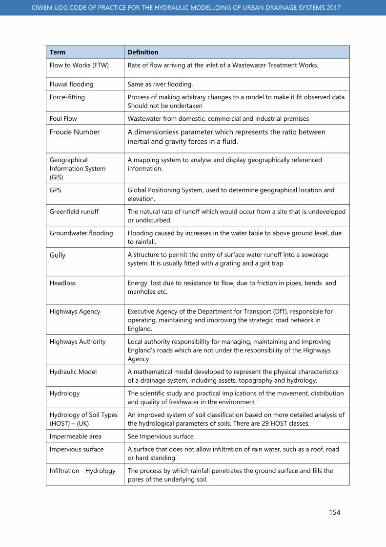
154
CIWEM UDG CODE OF PRACTICE FOR THE HYDRAULIC MODELLOING OF URBAN DRAINAGE SYSTEMS 2017
Term Definition
Flow to Works (FTW) Rate of flow arriving at the inlet of a Wastewater Treatment Works.
Fluvial flooding Same as river flooding.
Force-fitting Process of making arbitrary changes to a model to make it fit observed data. Should not be undertaken
Foul Flow Wastewater from domestic, commercial and industrial premises
Froude Number A dimensionless parameter which represents the ratio between inertial and gravity forces in a fluid.
Geographical Information System (GIS)
A mapping system to analyse and display geographically referenced information.
GPS Global Positioning System, used to determine geographical location and elevation.
Greenfield runoff The natural rate of runoff which would occur from a site that is undeveloped or undisturbed.
Groundwater flooding Flooding caused by increases in the water table to above ground level, due to rainfall.
Gully A structure to permit the entry of surface water runoff into a sewerage system. It is usually fitted with a grating and a grit trap
Headloss Energy lost due to resistance to flow, due to friction in pipes, bends and manholes etc.
Highways Agency Executive Agency of the Department for Transport (DfT), responsible for operating, maintaining and improving the strategic road network in England.
Highways Authority Local authority responsibility for managing, maintaining and improving England’s roads which are not under the responsibility of the Highways Agency
Hydraulic Model A mathematical model developed to represent the physical characteristics of a drainage system, including assets, topography and hydrology.
Hydrology The scientific study and practical implications of the movement, distribution and quality of freshwater in the environment
Hydrology of Soil Types (HOST) – (UK)
An improved system of soil classification based on more detailed analysis of the hydrological parameters of soils. There are 29 HOST classes.
Impermeable area See Impervious surface
Impervious surface A surface that does not allow infiltration of rain water, such as a roof, road or hard standing.
Infiltration - Hydrology The process by which rainfall penetrates the ground surface and fills the pores of the underlying soil.

155
CIWEM UDG CODE OF PRACTICE FOR THE HYDRAULIC MODELLOING OF URBAN DRAINAGE SYSTEMS 2017
Term Definition
Infiltration - Sewers The entry of groundwater into a sewer system through the pipe work, It may also include the entry of unplanned flows into a sewer system via manholes or misconnections.
Integrated Urban Drainage (IUD)
Approach to planning or managing an urban drainage system which leads to an understanding of how different physical components interact
intensity-duration-frequency (IDF)
The relationship between rainfall intensity (amount per unit of time), rainfall duration (total time over which rainfall occurs) and frequency (return interval) at which the intensity-duration relationship is expected to recur.
Intermittent Discharge Non continuous discharge from the Wastewater Network to a watercourse. This will include discharges from a CSO, EO or a storm tank.
Internal Drainage Boards (IDBs)
Independent bodies responsible for land drainage in areas of special drainage need that extends to 1.2 million hectares of lowland England.
Inundation The flooding of an area with water.
Joint Probability Analysis of the probability of two or more conditions which affect risk occurring concurrently.
Land Use Catchments zoned based on ergonomic, geographic or demographic use of land, such as residential, industrial, agricultural and/or commercial, together with the drainage system type.
LiDAR Light Detection and Ranging. Ground elevation data
Link An element of a model linking two nodes. This could be a conduit or a feature, for example a weir or a control.
Main River Main rivers are usually larger streams and rivers, but also include smaller watercourses of strategic drainage importance. The Environmental Regulator has responsibility for main rivers and are designated by Defra.
Major drainage system The above ground drainage systems. These would include watercourses and rivers which form the principal drainage pathways for catchments and the overland flow paths on river flood plains and the urban environment. These are broadly classified into two types: within channel flows or overland flow paths.
Manhole Headloss Energy losses at a manhole.
MCERTS (UK) Environment Agency Monitoring Certification Scheme for equipment, personnel and organisations. In this case certified flow monitoring at WwTW
Minor drainage system The underground piped drainage systems which are typically sewers but could also be culverted watercourses or highway drains.
Misconnections Mis-connections are surface water connections to a foul system or vice versa by householders or commercial premises;
Model A numerical representation of physical assets and processes
Model Maintenance The process of maintaining hydraulic models for future use on
Modelling Team Team responsible for carrying out the modelling project

156
CIWEM UDG CODE OF PRACTICE FOR THE HYDRAULIC MODELLOING OF URBAN DRAINAGE SYSTEMS 2017
Term Definition
Nash-Sutcliffe Efficiency Coefficient (NSEC)
The Nash–Sutcliffe model efficiency coefficient is used to assess the predictive power of hydrological models.
Flood Authority Bodies having overall for flooding, e.g. in England this would be the Environment Agency at a National Level and Local Authorities and Internal Drainage Boards at a local level.
Node A point in a modelled drainage system that receives runoff and other inflows, that connects links together, or that discharges water out of the system. Nodes can be manholes, junctions, storage units or outfalls. Every modelled link is attached to both an upstream and downstream node.
OFWAT Economic Water Industry Regulator for England and Wales
Operations The process of operating and maintaining a drainage system, and the part of an organisation that undertakes this.
Ordinary Watercourse An ordinary watercourse is any other river, stream, ditch, cut, sluice, dyke or non-public sewer which is not a Main River. The local authority or Internal Drainage Board has powers for such watercourses.
Overflow A point where excess flow can spill from one drainage type to another.
Overland Flow Path The path that runoff follows as it flows over a surface until it reaches a collection channel or drain.
Partially Separate Drainage System
A drainage system where there is a mixture of a combined system and a separate system, usually with the inclusion of separate surface water sewers.
Pass Forward Flow (PFF) Flow that continues on through the network after passing through a network ancillary
Pass forward flow at first spill
Continuation flow from a CSO at the moment the overflow spills
Per capita consumption (PCC) (G)
The amount of domestic and unmeasured commercial water returned as flow to sewer, generally expressed as units of litres/head/day.
Pervious (Permeable) Surface
A surface that allows water to infiltrate into the soil below it, such as a natural undeveloped area, grass verges or a gravel roadway.
Pluvial Flooding Flooding that results from rainfall-generated overland flow, before the runoff enters any watercourse or sewer.
Postal address point data (PAF) – (UK))
The Postcode Address File (PAF) is a database which contains all known "Delivery Points" and postcodes in the United Kingdom
Preissmann Slot The Preissmann slot is a fictitious slot above the soffit of a pipe to allow the use of open channel flow methods to simulate pipe flow in surcharged conditions. As this introduces additional conduit area in the model, there needs to be a reduction in system storage to compensate for the slot.
Rainfall Induced Infiltration
Non-continuous storm flows that enter a sewer due to inflow from land drainage as well as increased infiltration from subsurface flows through cracked pipes and leaking joints etc.

157
CIWEM UDG CODE OF PRACTICE FOR THE HYDRAULIC MODELLOING OF URBAN DRAINAGE SYSTEMS 2017
Term Definition
Return Period The expected average time between the exceedance of a particular threshold. Frequently used to express the frequency of occurrence of an event e.g. rainfall or flooding.
Revitalised Flood Hydrograph Models (ReFH2)
A model to generate flood peak flows and hydrographs from given rainfall events for both catchments and development sites.
River flooding Occurs when river flow exceeds the channel capacity due to rainfall, covering the adjacent floodplain with water.
RTC Real Time Control
Runoff Rain and surface water that does not percolate into the ground and flows over the surface to a sink, such as a drainage system inlet, watercourse or surface water body
Scattergraph A Scattergraph has points that show the relationship between two sets of data. In this case the comparison of observed depth and flow or velocity and flow. Used in the assessment of the consistency of recorded flow survey data.
Screen In wastewater network a device used to remove solid material, either from continuation flow at a WwTW or from spill pipes at CSOs. In a watercourse used to prevent debris from entering a culvert.
Section 105a Sewer (England and Wales)
Previously private sewers and drains that became vested in the Water Utilities under the “Water Industry (Schemes for Adoption of Private Sewers 2011)”
Separate Drainage System
A two pipe drainage system with one pipe taking foul flows and a second pipe taking surface water (storm) flows.
Setting Continuation flow at which an overflow starts to spill.
Sewer Quality Model Model which can simulate the flows and the concentrations of various indicators of the pollutant load in sewage as it flows through the sewer system.
Sewerage Risk Manual A web based process defining a risk based framework to capital maintenance and investment for wastewater network assets. Previously known as the Sewer Rehabilitation Manual (SRM)
Sewerage Management Plan (SMP)
A business plan covering all aspects of sewerage performance related expenditure for a defined number of years, covering a complete drainage area and considering all stakeholders
Sewerage Risk Manual (SRM)
A web based process defining a risk based framework to capital maintenance and investment for wastewater network assets. Previously known as the Sewer Rehabilitation Manual (SRM)
Sewers for Adoption Standard for new drainage systems in England & Wales so that they can be adopted by a WaSC.
Sewers for Scotland Standard for new drainage systems in Scotland

158
CIWEM UDG CODE OF PRACTICE FOR THE HYDRAULIC MODELLOING OF URBAN DRAINAGE SYSTEMS 2017
Term Definition
Slow Response flows Flow entering the sewerage system from pervious surfaces, either directly or as a result of seepage through the ground into the sewerage network. Typically when water enters the sewer a few hours after the onset of rainfall and persists for a significant amount of time after the event.
Soil Moisture Deficit The difference between a soil’s current moisture content and its moisture content at saturation.
Stakeholder An individual or group with an interest in, or having an influence over, the success of a proposed project or other course of action.
Strategic Flood Risk Assessment (SFRA)
Provides information on areas at risk from all sources of flooding. The SFRA should form the basis for flood risk management decisions and inputs into development allocation and control decisions.
Subcatchment A sub-area of a larger catchment area whose runoff flows into a single drainage pipe or channel.
Subcritical flow Water depth is greater than critical depth. In practice this leads to tranquil flow and the depth is controlled at the downstream end of the section.
SuDS Sustainable drainage systems: a sequence of management practices and control measures designed to mimic natural drainage processes by allowing rainfall to infiltrate, and by attenuating and conveying surface water runoff slowly compared to conventional drainage.
Supercritical flow Water depth is less than critical depth. High velocity results. Depth is controlled at the upstream end of the section.
Surcharge Condition in which the hydraulic gradient is higher than the soffit of a pipe. The flow is pressurised.
Surface flooding Flooding from sewers, drains, small water courses and ditches that occur as a result of heavy rainfall and exceedance of the local drainage capacity. May occur from any component of the urban drainage system.
Surface Water Management Plans (SWMPs)
Vehicle through which urban flood risk will be assessed, managed and resolved in the future within England and Wales.
System Storage Compensation
An allowance included in a model for unaccounted for storage in a drainage system, generally from un-modelled local house connections or elements of the system that have been removed as part of a simplification process.
Time Series Rainfall (TSR)
A series of rainfall data (over a number of years) used with sewer models to analyse the performance of a sewer system. Can be stochastic or historical data.
Topographical Surveys Manual surveys carried out on surface topography where higher accuracy is required than can be obtained using other digital methods.
Trade Effluent Permit (UK)
A permit given to an industrial user for discharging flow to the public sewer or watercourse. Permits usually have a daily maximum flow and a maximum peak flow.
Trade Flows Flow to sewer from industrial premises, with or without a permit.

159
CIWEM UDG CODE OF PRACTICE FOR THE HYDRAULIC MODELLOING OF URBAN DRAINAGE SYSTEMS 2017
Term Definition
Unsatisfactory Intermittent Discharge (UID)
Intermittent discharge considered unsatisfactory by the Environmental Regulator requiring upgrade.
Urban Creep Urban Creep is the progressive loss of permeable surfaces within urban areas creating increased runoff, generally due to small extensions, conservatories and paving over garden areas
Urban Pollution Management (UPM)
Urban Pollution Management (UPM) is defined as the management of wastewater discharges from sewer and sewage treatment systems under wet weather conditions such that the requirements of the receiving water are met in a cost effective way. The3rd edition of the manual is available from the Foundation for Water Research (FWR).
Validation Process of determining the degree to which a model or simulation is an accurate representation of the ‘real world’ from the perspective of its intended use.
Verification Process of comparing a model against independent data to determine its accuracy. Any changes to the model should be made only where this reflects the physical state of the sewer system and not solely to make the model fit the verification data
WaPUG Previous name for CIWEM Urban Drainage Group, with a long history of promoting best practice in the field of urban drainage.
Water and Sewerage Company (WaSC)
Ten regional water and sewerage companies (WaSCs) are licensed for England and Wales, set up under the Water Industry Act 1991. For the purposes of this Code the term includes any organisation responsible for the management of the sewerage system, including Scottish Water and Northern Ireland Water.
Watercourse A natural or artificial channel along which water flows
Winter Rain Acceptance Potential (WRAP)
A classification system of soils based on their hydrological response, developed as part of the Flood Studies Report. There are five classes of soil.
WwTW Wastewater Treatment Work (Sewage Works)
Abbreviations
Term Definition
1D One dimensional
2D Two dimensional
API Antecedent Precipitation Index
API30 Antecedent Precipitation Index 30 Days
API5 Antecedent Precipitation Index 5 Days
BGS British Geological Survey
CAS Contributing Area Survey (See IAS)

160
CIWEM UDG CODE OF PRACTICE FOR THE HYDRAULIC MODELLOING OF URBAN DRAINAGE SYSTEMS 2017
Term Definition
CCTV Closed Circuit Television
CDA Critical Duration Assessment
CIRIA Construction Industry Research and Information Association.
CIWEM Chartered Institution of Water and Environmental Management
CIWEM UDG CIWEM Urban Drainage Group
CoP Code of Practice
CSO Combined Sewer Overflow
D/S Downstream
DAP Drainage Area Plan
DAS Drainage Area Study
DEFRA Department for Environment, Food and Rural Affairs
DEM Digital Elevation Model
DG5 Director General 5 Indicator (Internal Flooding)
DM Depth Monitor
DTM Digital Terrain Model
DWF Dry Weather Flow
EA Environment Agency
EDM Event Duration Monitoring
EO Emergency Overflow
FEH Flood Estimation Handbook
FFT Flow to Full Treatment
FM Flow Monitor
FSR Flood Studies Report
FTW Flow to Works
GIS Geographical Information System
GPS Global Positioning System
HOST The Hydrology of Soil Types Classification
IA Impermeable Area
IAS Impermeable Area Survey (See CAS)
ICG Internal Condition Grade
ID Intermittent Discharge
IDF intensity-duration-frequency
l/h/d Litres per head per day
LAMP Local Asset Management Plan

161
CIWEM UDG CODE OF PRACTICE FOR THE HYDRAULIC MODELLOING OF URBAN DRAINAGE SYSTEMS 2017
Term Definition
LEAP Local Environment Agency Plan
LiDAR Light Detection and Ranging.
LOS Level of Service
MBV Model Build & Verification
MCERTS Environment Agency Monitoring Certification Scheme for equipment, personnel and organisations. In this case flow monitoring at WwTW.
MH Manhole
NGR National Grid Reference
NIEA Northern Ireland Environment Agency
NRW Natural Resources Wales
NSEC Nash-Sutcliffe Efficiency Coefficient
NRV Non Return Valve
NTS Not To Scale
OFWAT The economic regulator of the water sector in England and Wales
O/S Outside
ONS Office of National Statistics
OS Ordnance Survey
PCC Per Capita Consumption (G)
PE Population Equivalent
PS Pumping Station
QA Quality Assurance
ReFH2 Revitalised Flood Hydrograph Model.
RG Rain Gauge
RPA Return Period Analysis
RQO River Quality Objective
RTC Real Time Control
SAAR Standard Average Annual Rainfall
SASR Standard Average Summer Rainfall
SEPA Scottish Environment Protection Agency
SIRS Sewerage Incident Reporting System
SMD Soil Moisture Deficit
SPG Structural Performance Grade
SPS Sewage Pumping Station
SRM Sewerage Risk Manual

162
CIWEM UDG CODE OF PRACTICE FOR THE HYDRAULIC MODELLOING OF URBAN DRAINAGE SYSTEMS 2017
Term Definition
SS Suspended Solids
TE Trade Effluent
TPS Terminal Pumping Station
TSR Time Series Rainfall
U/S Upstream
UCWI Urban Catchment Wetness Index
UID Unsatisfactory Intermittent Discharge
UKWIR UK Water Industry Research
UPM Urban Pollution Management
WaPUG Wastewater Planning Users Group
WIC The Water Industry Commission for Scotland.
WQ Water Quality
WRAP Winter Rainfall Acceptance Potential
WRc Water Research Council
WwTW Waste Water Treatment Works

Page 163 of 169
Urban Drainage Group


