APPENDIX JP% Loss-of-Containment Causes in the Chemical Industry Plant Inventory Discharged to Environment Due to Loss of Containment (Note: This cannot presume to be an exhaustive list of causes.) L CONTAINMENT LOST VIA AN "OPEN-END" ROUTE TO ATMOSPHERE A. Due to genuine process reliefer dumping requirements B. Due to maloperation or equipment in service, e.g., spurious relief valve opera- tion or rupture disk failure C. Due ttfoperator error, e.g., drain or vent valve left open, misrouting of materials, tank overfilled, unit opened up under pressure, etc. IL CONTAINMENT FAILURE UNDER DESIGN OPERATING CONDITIONS DUE TO IMPERFECTIONS IN THE EQUIPMENT A. Imperfections arising prior to commissioning and not detected before start-up (due to poor inspection or testing procedures) 1. Equipment inadequately designed for proposed duty, e.g., wrong materials specified, pressure ratings of vessel or pipework inadequate, temperature rat- ings inadequate, etc. 2. Defects arising during manufacture, e.g., wrong materials used, poor work- manship, poor quality control, etc. 3. Equipment damage or deterioration in transit or during storage. 4. Defects arising during construction, e.g., welding defects, misalignment, wrong gaskets fitted, etc. B. Imperfections due to equipment deterioration in service and not detected before the effect becomes significant (due to inadequate monitoring procedures in those cases where deterioration is gradual 1. Normal wear and tear on pump or agitators seals, valve packing, flange gas- kets, etc. 2. Internal and/or external corrosion, including stress corrosion cracking 3. Erosion or thinning 4. Metal fatigue or vibration effects
Transcript
APPENDIX JP%
Loss-of-Containment Causes in the
Chemical Industry
Plant Inventory Discharged to Environment Due to Loss of Containment
(Note: This cannot presume to be an exhaustive list of causes.)
L CONTAINMENT LOST VIA AN "OPEN-END" ROUTE TO ATMOSPHEREA. Due to genuine process reliefer dumping requirementsB. Due to maloperation or equipment in service, e.g., spurious relief valve opera-
tion or rupture disk failureC. Due ttfoperator error, e.g., drain or vent valve left open, misrouting of materials,
tank overfilled, unit opened up under pressure, etc.
IL CONTAINMENT FAILURE UNDER DESIGN OPERATINGCONDITIONS DUE TO IMPERFECTIONS IN THE EQUIPMENT
A. Imperfections arising prior to commissioning and not detected before start-up(due to poor inspection or testing procedures)1. Equipment inadequately designed for proposed duty, e.g., wrong materials
specified, pressure ratings of vessel or pipework inadequate, temperature rat-ings inadequate, etc.
2. Defects arising during manufacture, e.g., wrong materials used, poor work-manship, poor quality control, etc.
3. Equipment damage or deterioration in transit or during storage.4. Defects arising during construction, e.g., welding defects, misalignment,
wrong gaskets fitted, etc.B. Imperfections due to equipment deterioration in service and not detected before
the effect becomes significant (due to inadequate monitoring procedures inthose cases where deterioration is gradual1. Normal wear and tear on pump or agitators seals, valve packing, flange gas-
kets, etc.2. Internal and/or external corrosion, including stress corrosion cracking3. Erosion or thinning4. Metal fatigue or vibration effects
5. Previous periods of gross maloperation, e.g., furnace operation at above thedesign tube skin temperature ("creep")
6. Hydrogen embrittlementC. Imperfections arising from routine maintenance or minor modifications not car-
ried out correctly—poor workmanship, wrong materials, etc.
III. CONTAINMENT FAILURE UNDER DESIGN OPERATINGCONDITIONS DUE TO EXTERNAL AGENCIES
A. Impact damage, such as by cranes, road vehicles, excavators, machinery associ-ated with the process, etc.
B. Damage by confined explosions due to accumulation and ignition of flammablemixtures arising from small process leaks, e.g., flammable gas build-up in ana-lyzer houses, in enclosed drains, around submerged tanks, etc.
C. Settlement of structural supports due to geological or climatic factors or failureof structural supports due to corrosion, etc.
D. Damage to tank trucks, rail cars, containers, etc., during transport of materialson-or off-site
E. Fire exposureF. Blast effects from a nearby explosion (unconfined vapor cloud explosion, burst-
ing vessel, etc.), such as blast overpressure, projectiles, structural damage,domino effects, etc.
G. Natural events (acts of God) such as windstorms, earthquakes, floods, lightning,etc.
IV. CONTAINMENT FAILURE DUE TO DEVIATIONS IN PLANTCONDITIONS BEYOND THE DESIGN LIMITS
A. Overpressuring of equipment1. Due to a connected pressure source
a. gas pressure source(1) gas breakthrough into downstream low-pressure equipment due to
failure of a pressure or level controller, isolation valve opened in error,etc.
(2) pressurized backflow into low-pressure equipment, e.g., due to com-pressor failure
b. liquid pressure source(1) pumping up of blocked-in gas spaces(2) hydraulic overpressuring due to a block-in condition downstream(3) excessive surge or hammer, such as by sudden valve closure on liquid
transfer line2. Due to rising process temperature
a. loss of cooling(1) loss of coolant flow, e.g., to a reactor cooler, to a distillation column
condenser, etc.(2) elevated coolant temperature, e.g., loss of cooling water fans, etc.
b. excessive heat input (thermal)(1) heater control faults, such as on steam or hot oil heated systems
c. excessive heat generation (chemical)(1) reaction runaway, e.g., due to loss of reaction diluent, high feed to
inadequate mixing or temporary los of reaction subsequently leadingto a runaway, etc.
(2) exotherming due to ingress of catalytic impurities, e.g., backflowfrom ethylene oxide consumer unit into feed tank
(3) exotherming due to mixing of incompatible chemicals, e.g. H2SO4
with NaOH(4) exothermic decomposition of thermally unstable or explosive material
such as peroxides, e.g., due to temperature rise, overconcentration, ordeposition on hot surfaces
3. Due to an internal explosion arising from formation and ignition of flamma-ble gas mixtures, mists, or dusts.a. ingress of air, e.g., due to inadequate purging of equipment at plant start-
up, due to loss of nitrogen purge on flare headers, storage tanks, centrifugesystems, dryers, etc.
b. loss of critical inert diluent, e.g., loss of nitrogen padding on an ethyleneoxide storage tank, los of nitrogen to the make-up section of a nitrogen/airsolids conveying system
c. failure of explosion suppressantsd. flammable excursion in oxidation processes, e.g., due to high air or oxygen
rates, or loss of conversion4. Due to physically or mechanically induced forces or stresses
a. expansion upon change of state, e.g., freezing of water in pipe runsb. thermal expansion of blocked-in liquids, e.g., in heat exchangers or long
pipe runsc. ingress of extraneous phases, e.g., gas compressor failure due to liquid
carry-through to machine suction, condensate hammer in steam lines, etc.D. Underpressuring of equipment (for equipment not capable of withstanding
vacuum)1. By direct connection to an ejector set or to equipment normally running
under vacuuma. due to equipment malfunction, e.g., loss of liquid seal due to failure of a
level controller causing vacuum to be applied upstream, etc.b. due to operator error, e.g., isolation valve left open, etc.
2. Due to the movement or transfer of liquidsa. pumping out of tanks or vesselsb. emptying or draining elevated blocked-in equipment under gravity
3. Due to cooling of gases or vaporsa. condensation of condensible vapors, e.g., vessel blocked-in after steamingb. cooling of noncondensable gases or vapors, e.g., storage tank by heavy
rainfall in summer4. Due to solubility effects, e.g., dissolution of gases in liquids
C. High metal temperature (causing loss of strength)1. Fire under equipment, e.g., due to spillage, pump leak, etc.
2. Flame impingement causing local overheating, e.g., on furnaces due to mis-alignment or maladjustment of burners
3. Overheating by electric heaters, e.g., due to failure of high temperaturecutout
4. Inadequate flow of fluid via heated equipment, e.g. furnace tube failure onloss of hot oil flow
5. Higher flow rate or higher temperature of the hotter stream, or lower flowrate or higher temperature of the colder stream, via a heat exchanger
D. Low metal temperature (causing cold embrittlement and overstressing)1. Overcooling by refrigeration units, e.g., due to control faults, wrong refriger-
ant, etc.2. Incomplete vaporization and/or inadequate heating of refrigerated material
before transfer into equipment of inadequate temperature rating, e.g., due tocontrol faults on a liquid ethylene vaporization unit
3. Loss of system pressure on units handling liquids of low boiling pointE. Wrong process materials or abnormal impurities (causing accelerated corrosion,
chemical attack of seals or gaskets, stress corrosion cracking, embrittlement, etc.)1. Variations in stream compositions outside design limits2. Abnormal impurities introduced with raw materials or wrong raw materials3. By-products of abnormal chemical reactions4. Oxygen, chlorides, or other impurities remaining in equipment at start-up
due to inadequate evacuation or decontamination5. Impurities entering process from atmosphere, service connections, tube
leaks, etc. during operation
APPENDIX D
Training Programs
A thorough understanding of the methodologies of CPQBA is essential to obtainhigh-quality risk estimates. As stated in the Preface, there is no substitute for experi-ence. Experience can come only from training and repeated practice. Competence,much less expertise, cannot be expected following exposure to only a brief introductorycourse. This appendix addresses who should be trained, what material should be cov-ered, and how much time is needed for training.
B.I. Training Needs
The purpose of this section is to address the following questions:
• Who should be trained? (Section B.2)• What material should be covered:1 (Section B.3)• How much time is needed? (Section B.4)
and to offer some cautions and general guidance (Section B. 5) about the use of processengineers as risk analysts and the maintenance of experts' proficiency in CPQRA tech-niques.
B.2. Who Should Be Trained?
Individuals from line and staff groups who participate in CPQRA studies assume oneor more of the following functions:
• senior management• site or unit manager• risk analysis project manager• process engineer• risk analyst• risk methods development specialist.
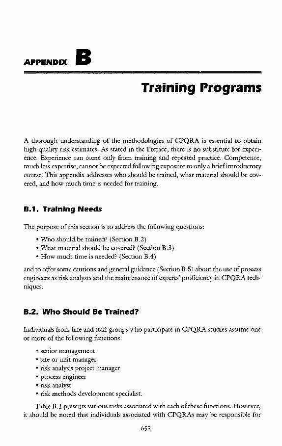
Table B.I presents various tasks associated with each of these functions. However,it should be noted that individuals associated with CPQRAs may be responsible for
tasks from several functions. The list of functions and their associated tasks (Table B.I)are for convenience only, to facilitate discussion of the training needs for members ofthe CPQRA team and other personnel.
The process of selecting people to participate in CPQRA studies or to perform thefunctions listed above, and the amount of training each person should receive are issuesthat are properly addressed through the development of a Risk Management Plan for anorganization. A discussion of the details of developing such a plan is beyond the scope of
TABLE B. 1 . Typical Task Profiles for CPQRA-Related Job Functions
Job function
Senior Management (corporatestaff)
Existing Site or Unit Management(plant staff) or New Site or UnitProject Management (engineeringstaff)
Risk Assessment Project Manager(plant staff or corporate staff)
• Be able to calculate the whole range of risk measures
• Provide advice on the interpretation of risk analysis results
• Provide training to company staff in CPQBA techniques
• Provide advice on wide range of CPQRA componenttechniques
• Develop or enhance CPQRA component techniques
• Provide training to company staff in CPQRA componenttechniques
these guidelines. However, it is clear that the training needs of each of the above func-tions differ in scope and intensity. Identifying the occupants for the above functions orthose members of the organization responsible for the tasks listed in Table B.I answersthe question "Who should be trained!1" In addition, useful involvement of operators andmaintenance personnel in any level of CPQEA is an informal sort of training that can behelpful in expanding their thinking, even though formal training is not provided.
B.3. What Material Should Be Covered?
CPQBA training should cover the following areas (at least):
• Hazard Identification. Detailed training should cover at least one formal hazardidentification methodology (e.g., HAZOP, FMEA), plus a brief exposure toother techniques.
• Consequence Modeling. All of the physical models identified in this documentshould be reviewed. Special attention needs to be given to dense gas dispersionand UVCE, as these are less familiar concepts to many process engineers. Effectsmodeling should also be covered both in terms of human effects and structuraldamage. Instruction in the use of available computer tools may be beneficial.
• Frequency Modeling. The use of historical data in estimating incident frequenciesshould be covered, along with means to evaluate the suitability of such informa-tion. Sufficient training in FTA and ETA should be given so that process engi-neers are able to construct simple trees, to understand more complex treesdeveloped by others, and to spot potential errors in more complex structures.Instruction in the use of available computer tools may be beneficial. Other tech-niques such as human reliability analysis and the compilation and interpretationof raw reliability data are areas requiring highly specialized training.
• Risk Estimation and Presentation. Training should be provided in the calculationof common risk measures and in the combination of frequency and consequenceestimates to produce risk estimates.
• CPQRA Utilization. The uses of the estimates of risk produced by a CPQBAwithin an organization should be covered. These include ranking risk reductionmeasures, examining the utility of safety investment options, etc.
B.4. How Much Time Is Needed?
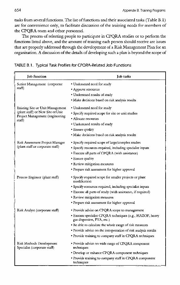
The time needed for training the CPQBA team can be estimated from the type of train-ing required for each function (Table B.2) and the estimated time required for eachtype of training (Table B.3). Of course, this can not be finalized until the compositionof the team is established.
In addition to the basic training shown in Table B.3, personnel who are to beexperts will need to improve and thereafter maintain their proficiency by advancedcourse work, monitoring current developments, working on CPQBAs, etc. Consider-ation of the number of topics and the number of references per topic in the related Top-
TABLE B.2. CPQRA Training Needs by Function
Training requirements*
Riskpresentation
Hazard Consequence Frequency andFunction Overview identification modeling modeling utilization
Senior Management I — — — I
Existing Site Unit Manger or I I I I INew Site/Unit ProjectManager
Risk Analysis Project C C C CManager
Process Engineer C C C C
Risk Analyst A A A A
Risk Methods Development A A A ASpecialist
"I, introductory level course; C, basic competence level course; A, advanced material level course(s).
ical Bibliography to be made available from CCPS should show the extent of theknowledge required by an expert. The cost and time required for creating an expertcannot usually be borne by one project, but must be a general overhead expense if an in-house analyst is to be available when needed. Expertise can be built through a series ofsmaller investments (short courses) over much longer periods than covered by a singleproject. This expertise must be maintained in a similar fashion.
B.5. Cautions and Guidance
When creating a master plan for CPQRAs there are two considerations: (1) avoidingthe assumption that knowledgeable process engineers are inherently able to perform allCPQBA functions without further training, and (2) maintaining the organization'sskills at all levels.
There is a temptation to assume that process engineers (in particular)-because oftheir expert knowledge of chemical process technology-are capable of undertakingcomprehensive consequence and frequency analyses without the guidance of a risk ana-lyst. This can lead to inaccurate or inadequate risk analyses, and process engineersshould not perform such work unguided until they have demonstrated the necessaryproficiency. Conversely, risk analysts cannot perform quality CPQRAs without work-ing closely with process engineers and plant personnel.
Maintaining the skills of senior management, and site or unit managers, is mainly amatter of training replacements when turnover occurs. Risk analysts, Risk methodsdevelopment specialists, and other specialists and experts maintain their skills by con-tinuing education, exercising their talents, etc.
APPENDIX W
Sample Outline for CPQRA Reports
The outline presented below will help accomplish the following functions of a CPQBAreport: (1) present the background and results of the CPQBA in a way that satisfies theneeds of the user while withstanding scrutiny and question, and (2) preserve the assess-ment in a retrievable form. Generally, the final report is the most retrievable documentfrom a CPQRA, and, this, should contain as many details as possible regarding the ana-lytical calculations, assumptions, and results (within the bounds of practicality).Ideally, it would be possible to regenerate or expand the assessment from this report.
Preface
Executive Summary
1. INTRODUCTION AND BACKGROUND1.1. Description of the System1.2. Purpose and Scope1.3. Definition and Function of Problem1.4. General Approach, Methods, and Analytical Techniques Used1.5. Organization of Report
2. HAZARDS IDENTIFICATION, SCREENING, AND PROBLEMPRIORITIZATION
3. EQUIPMENT AND HUMAN FAILURE, AND SITE DATA BASEDEVELOPMENT3.1. Applicable Industry Data3.2. Plant Operating and Incident Data3.3. Demographic Data3.4. Summary of Data Used for the Analysis
4. QUANTITATIVE SYSTEMS-FAILURE ANALYSIS4.1. System Description4.2. Systems Boundaries4.3. Specific Assumptions4.4. Results and Identified Problems
5. ANALYSIS OF CRITICAL HAZARD-CONSEQUENCES5.1. Summary of Analytical Methods and Limitations5.2. Specific Assumptions, Demography5.3. Results
6. DETERMINATION OF PLANT RISK6.1. Individual Risk6.2. Societal Risk
7. RESULTS AND RECOMMENDATIONS7.1. Results of Sensitivity Studies7.2. Summary of Major Recommendations (Design, Mitigating Measures,
Protective Actions, and Emergency Action Plans)7.3. Conclusions
APPENDICESA. System Documentation (e.g., Site Plans, PSdDs, Data Sheets, Operating
Procedures)B. General Assumptions and Boundary Conditions for the Systems AnalysisC. Supplemental Details Regarding Analytical Methodology/Computer Risk
All quantitative fault tree analysis methods are approximations of reality. By far thelargest contributions to error and uncertainty result from qualitative aspects of faulttree analysis and arise from
1. Lack of understanding of the system modeled, including all possible failuremechanisms (what is not included in the analysis because experience and/orjudgment are deficient);
2. Incorrect fault tree logic describing the system failures (if the logic is incorrectthen quantitative evaluation by any method will be incorrect);
3. Lack of understanding of or improper accounting for common cause failures.
In constructing a fault tree, the analyst usually follows a gate-by-gate approach.The fault tree developed consists of many levels of basic events and subevents linkedtogether by AND gates and OR gates. Minimal cut set analysis rearranges the fault treeso that any basic event that appears in different parts of the fault tree is not "doublecounted" in the quantitative evaluation. The result of minimal cut set analysis is a newfault tree, logically equivalent to the original, consisting of an OR gate beneath the topevent, whose inputs are the minimal cut sets. Each minimal cut set is an AND gate con-taining a set of basic inputs necessary and sufficient to cause the top event.
Some advantages and disadvantages of gate-by-gate and minimal cut set methodsinclude
1. Normal gate-by-gate methods are not as exact as minimal cut set methods. Spe-cial formulas may be required, for example, when failure rates or demand ratesare very high. Simple gate-by-gate methods cannot calculate the wide range ofreliability parameters generated by minimal cut set methods. More advancedgate-by-gate methods (Doelp et al, 1984) can overcome this deficiency.
2. Events that occur in different branches of the tree are treated correctly by mini-mal cut set analysis. Gate-by-gate methods require special efforts in construct-ing a tree that does not contain repeated events. Any repeated events notremoved will introduce a bias (positive or negative) in the results.
3. Gate-by-gate methods may make it easier to identify those subevents or basicevents that are the major contributors to the top event. Cut set methods calcu-late reliability parameters for the top event only and use other parameters suchas importance of identify major contributors to the top event. It is possible toseparately calculate reliability parameters for subevents using minimal cut setmethods if it is important to determine these parameters for subevents.
There are trade-offs in the selection of which approach to use. Simple gate-by-gatecalculations can rapidly produce results using hand calculations. Minimal cut set meth-ods use computer programs that are well developed and eliminate effects of repeatedevents. As fault trees become larger in size computerized methods become more attrac-tive, particularly when a large number of alternatives are to be evaluated.
D.2. Minimal Cut Set Analysis
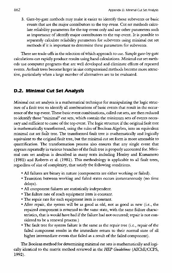
Minimal cut set analysis is a mathematical technique for manipulating the logic struc-ture of a fault tree to identify all combinations of basic events that result in the occur-rence of the top event. These basic event combinations, called cut sets, are then reducedto identify those "minimal53 cut sets, which contain the minimum sets of events neces-sary and sufficient to cause of the top event. The logic structure if the original fault treeis mathematically transformed, using the rules of Boolean Algebra, into an equivalentminimal cut set fault tree. The transformed fault tree is mathematically and logicallyequivalent to the original fault tree, but the minimal cut set form is more amenable toquantification. The transformation process also ensures that any single event thatappears repeatedly in various branches of the fault tree is properly accounted for. Mini-mal cuts set analysis is described in many texts including Henley and Kumamoto(1981) and Roberts et al. (1981). This methodology is applicable to all fault trees,regardless of size of complexity, that satisfy the following conditions.
• All failures are binary in nature (components are either working or failed).• Transition between working and failed states occurs instantaneously (no time
delays).• All component failures are statistically independent.• The failure rate of reach equipment item is constant.• The repair rate for each equipment item is constant.• After repair, the system will be as good as old, not as good as new (i.e., the
repaired component is returned to the same state, with the same failure charac-teristics, that is would have had if the failure had not occurred; repair is not con-sidered to be a renewal process.)
• The fault tree for system failure is the same as the repair tree (i.e., repair of thefailed component results in the immediate return to their normal state of allhigher intermediate events that failed as a result of the failed component).
The Boolean method for determining minimal cut sets is mathematically and logi-cally identical to the matrix method reviewed in the HEP Guidelines (AIChE/CCPS,1992).
D.3. Boolean Algebra
The logical structure of a fault tree can be expressed in terms of Boolean algebraic equa-tions. Boolean algebra is used to reduce equations composed of variables that can takeon only two values. It is commonly used to describe the operations of power switchinggrids, computer memories, or logic diagrams. Selected basic mathematical rules ofBoolean algebra are given in Table D.I. Conventionally, the symbol" +" is used to rep-resent the logical OR operator and the symbol"." is used to represent the logical ANDoperator. Roberts et al. (1981) present a more comprehensive rule tabulation and dis-cussion of Boolean algebra.
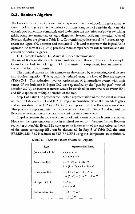
D.4. Sample Problem 1—Minimal Cut Set DeterminationThe use of Boolean algebra in fault tree analysis is first illustrated by a simple example.Consider the fault tree of Figure D.I. It consists of a top event, four intermediateevents, and four basic events.
The minimal cut sets for this example are determined by representing the fault treeas a Boolean equation. This equation is reduced using the laws of Boolean algebra(Table D.I). This reduction involves replacement of intermediate events with theircauses. If the fault tree in Figure D.I were quantified by the "gate-by-gate" method(Section 3.2.1), an incorrect answer would be obtained, because the basic events BEland BE 2 appear in multiple branches of the tree.
Step 1 of Table D.2 presents the Boolean representation of the top event in termsof intermediate events IEl and IE2. In step 2, intermediate event IEl (an AND gate)and intermediate event IE2 (an OR gate) are replaced by their Boolean equivalents.This process of replacing intermediate events is continued in Steps 3 and 4, until theBoolean representation of the fault tree contains only basic events.
Step 4 represents the top event in terms of basic events only. Each term is a cut set.However, the representation is not in minimal cut set form because further Booleanreduction is possible. Event BE4 appears twice in one term of the expression, and oneof the terms containing BEl can be eliminated. In Step 5 of Table D.2 the termBE3.BE4.BE4.BE2 is reduced to BE3.BE4.BE2 using the idempotent law (relation 4,
TABLE D. 1. Selected Rules of Boolean Algebra
Rule Mathematical form
Commutative Rule A-B = B-A
A+B=B+A
Associative Rule A • (B • C) = (A • B) - C
A + (B + C) = (A + B) + C
Distributive Rule A-(B + C)=A-B+A-C
A + (B - C ) = (A +B) - ( A + C)
Idempotent Rule A-A=A
A +A =A
Rule of Absorption A - (A + B) = A
A +A-B=A
Table D.I). In Step 6 of Table D. 2 the term BEl + BEl - BE2 is reduced to BEl usingthe law of absorption (Relation 5, Table D.I).
Step 7, the commutative law is used to reorder the basic events of the second term(putting them in numerical order for convenience).
The two terms in Step 7 (BEl and BE2 • BE3 • BE4) of Table D.2 are the minimalcut sets for the fault tree of Figure D.I. The occurrence of either of these two cuts setswill cause the top event of the simple fault tree of Figure D.I. The minimal cuts sets can
TABLE D.2. Reduction of Sample Fault Tree of Figure D. 1Using Boolean Algebra
Step Boolean representation
1 T = IEl + IE2
2 T= (BEl • BE2) + (BEl + IE3)
3 T = BEl • BE2 + BEl + (BE3 • BE4 • IE4)
4 T = BEl • BE2+ BEl + (BE3 • BE4 • BE4 • BE2)
5 T = BEl + BEl • BE2 + BE3 • BE4 - BE2
6 T = BEl + BE3•BE4•BE2
7 T = BEl + BE2 • BE3 • BE4
FIGURE D. 1. Simple fault tree.
TOPEVENT
INTERMEDIATEEVENT
IE-1INTERMEDIATE
EVENTIE-2
INTERMEDIATEEVENT
IE-3
INTERMEDIATEEVENT
IE-4
AND
BASICEVENT
BE2 .
BASICEVENT. BE4 ,
BASICEVENT. BE4 ,
BASICEVENT. BE3 .
BASICEVENT, BE1 .
BASICEVENT. BE2 .
BASICEVENT. BE1 .
AND
be used to create a new fault tree that is logically and mathematically identical to theoriginal. Figure D.2 presents the simple fault tree of Figure D.I in the equivalent mini-mal cut set form.
D.5. Sample Problem 2
For demonstration purposes the sample problem in Section 3.2.1 is recalculated usingthe minimal cuts set method. The treatment of Steps I5 2, and 3 (Figure 3.3) is thesame as discussed in Section 3.2.1, resulting in the fault tree of Figure 3.5. Step 4(Figure 3.3), qualitative examination of structure, and Step 5 (Figure 3.3), quantita-tive evaluation, are done using minimal cut set analysis.
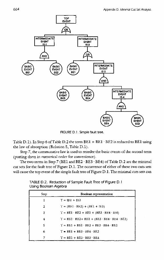
The same methods used in Sample Problem 1 are applied to the fault tree of Figure3.5. The Boolean algebra analysis of the fault tree is presented in Table D. 3. The 20 mini-mal cut sets identified in Step 6 of Table D.3 are listed in Table D.4. These are ranked interms of the number of basic events per cut set and are assigned reference numbers (Cl-C20). There are 5 single-event, 2 two-event, 12 three-event, and 1 five-event cut sets.The qualitative ranking of importance would assume that small cut sets (e.g., one andtwo events) are more likely to occur. However, this is not necessarily true in all cases. TheHEP Guidelines (AIChE/CCPS, 1985) discuss how other factors such as human error oractive and passive equipment failure can be used to further rank the cut sets. In Step 5(Figure 3.3), Quantitative Evaluation, it is shown that some larger cut sets in this exam-ple are more likely to occur than smaller ones.
Another objective of qualitative examination is to identify the susceptibility of thesystem to common-cause failures. As discussed in Section 3.2.1, several factors can leadto common-cause failure including:
• operator error• common manufacturer• local environmental factors• proximity of common equipment items• loss of a utility.
TOPEVENT
MINIMALCUT SET
MCS1
MINIMALCUT SET
MCS2
BASICEVENT
BE1BASICEVENT
BE2
BASICEVENT
BE3
BASICEVENT
BE4
AND
FIGURE D.2. Simple fault tree transformed into minimal cut sets.
" Every term of the final expansion is a minimal cut set (Table D.4). T, top event; M, intermediate event; B, basicevent.
The susceptibility to common-cause failure due to human error for one of the cutsets is illustrated as follows. Events B15, B16, B17, B18, and B21 are associated withhuman errors. Examining the cut sets (Table D.4), C8 contains two of the basic eventsassociated with human error (B 15, B16). Hence, this cut set is susceptible to humanerror. An inexperienced operator, who unloads the truck into the tank when there isinsufficient volume to receive it (B 15), might also not respond to the LIA-I high levelalarm (B 16).
Thus, these two events may not be truly independent because the same inexperi-enced operator is involved in both events. Their combined probability may be substan-tially higher than the 1 X 10~2 • 1 X 10"4 assuming independence.
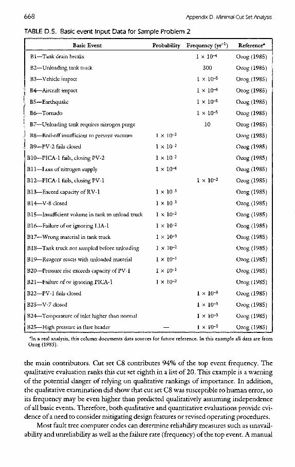
STEP 5. QUANTITATIVE EVALUATION OFSAMPLE PROBLEM 2 FAULT TREEThe approach described here is based on simple assignment of probabilities and fre-quencies to Basic events in the minimal cut sets. A more detailed treatment is reviewedin Appendix E. Table D.5 presents the frequency and probability data for the basicevents (from Figure 3.5). Table D.6 summarizes the calculated frequency of occur-rence of the minimal cuts sets. A calculation for Cut Set 8 in table D.5 is provided fordemonstration:
From Table D.4: C8 = B2 • B15 • B16From Table D.5: B2 = 300/year, B15 = 1 X 1(T2, B16 = 1 x 1(T2
Cut Set Frequency (Table D.6): C8 = B2 • B15 • B16= 300/yr • 1 x 1(T2 • 1 x 1(T2
= 3 x l(T2/yr
TABLE D.3. Minimal Cut Set Determination Steps3
Step Boolean expression for top event (T) of Figure 3.5
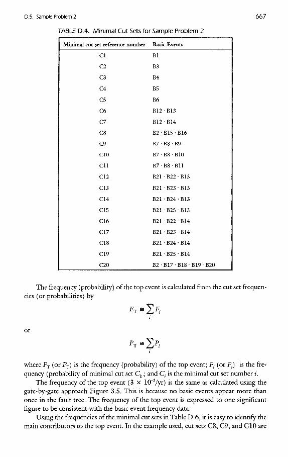
The frequency (probability) of the top event is calculated from the cut set frequen-cies (or probabilities) by
^T-5>,-i
or
*T -5>,*
where .FT (or P7) is the frequency (probability) of the top event; JF- (or P-) is the fre-quency (probability of minimal cut set Ck; and C- is the minimal cut set number i.
The frequency of the top event (3 x 10~2/yr) is the same as calculated using thegate-by-gate approach Figure 3.5. This is because no basic events appear more thanonce in the fault tree. The frequency of the top event is expressed to one significantfigure to be consistent with the basic event frequency data.
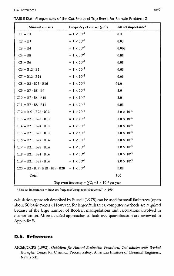
Using the frequencies of the minimal cut sets in Table D.6, it is easy to identify themain contributors to the top event. In the example used, cut sets C8, C9, and ClO are
TABLE D.4. Minimal Cut Sets for Sample Problem 2
Minimal cut set reference number Basic Events
TABLE D.5. Basic event Input Data for Sample Problem 2
Basic Event Probability Frequency (yr'1) Reference*
Bl-Tank drain breaks 1 X lO"4 Ozog (1985)
B2—Unloading tank truck 300 Ozog (1985)
B3—Vehicle impact 1 x 10'5 Ozog (1985)
B4—Aircraft impact 1 X 10~6 Ozog (1985)
B5—Earthquake 1 X 10~5 Ozog (1985)
B6—Tornado 1 X 10~5 Ozog (1985)
B7—Unloading tank requires nitrogen purge 10 Ozog (1985)
B8—Boil-off insufficient to prevent vacuum 1 x 10~2 Ozog (1985)
B9—PV-2 fails closed 1 x 10~2 Ozog (1985)
BIO—PICA-I fails, closing PV-2 1 x 10'2 Ozog (1985)
BIl—Loss of nitrogen supply 1 x 1O-4 Ozog (1985)
B12—PICA-I fails, closing PV-I 1 x 10~2 Ozog (1985)
B13—Exceed capacity of RV-I I x 10~3 Ozog (1985)
B14—V-8 closed 1 x IQ-3 Ozog (1985)
B15—Insufficient volume in tank to unload truck 1 x 10~2 Ozog (1985)
B16—Failure of or ignoring LIA-I 1 x 10~2 Ozog (1985)
B17—Wrong material in tank truck 1 x IO"3 Ozog (1985)
B18—Tank truck not sampled before unloading 1 X 10~2 Ozog (1985)
B19—Reagent reacts with unloaded material 1 X 10"1 Ozog (1985)
B20—Pressure rise exceeds capacity of PV-I 1 x 10'1 Ozog (1985)
B21—Failure of or ignoring PICA-I 1 x 10~2 Ozog (1985)
B22—PV-I fails closed 1 X 10~3 Ozog (1985)
B23—V-7 closed 1 x IQ-* Ozog (1985)
B24—Temperature of inlet higher than normal 1 X 10~3 Ozog (1985)
B25—High pressure in flare header — I x IO"3 Ozog (1985)
"In a real analysis, this column documents data sources for future reference. In this example all data are fromOzog (1985).
the main contributors. Cut set C8 contributes 94% of the top event frequency. Thequalitative evaluation ranks this cut set eighth in a list of 20. This example is a warningof the potential danger of relying on qualitative rankings of importance. In addition,the qualitative examination did show that cut set C8 was susceptible to human error, soits frequency may be even higher than predicted qualitatively assuming independenceof all basic events. Therefore, both qualitative and quantitative evaluations provide evi-dence of a need to consider mitigating design features or revised operating procedures.
Most fault tree computer codes can determine reliability measures such as unavail-ability and unreliability as well as the failure rate (frequency) of the top event. A manual
TABLE D.6. Frequencies of the Cut Sets and Top Event for Sample Problem 2
Minimal cut sets Frequency of cut set (yr"1) Cut set importance"
Cl = Bl = 1 x 10"4 0.3
C2 = B3 = 1 x ID"5 0.03
C3 = B4 = 1 x IQ-6 0.003
C4 = B5 = 1 x IQ-5 0.03
C5 = B6 = 1 x 10~5 0.03
C6 = B12 • Bl = 1 x 10~5 0.03
C7 = B12-B14 = 1 x 10'5 0.03
C8 = B2 • B15 • B16 = 1 x 10~2 94.0
C9 = B7 • B8 • B9 = 1 X 10~3 3.0
ClO = B7 • B8 • BlO = 1 x 10"3 3.0
CIl = B 7 - B 8 - B 1 1 = 1 x 10~5 0.03
C12 = B21 • B22 • B13 = 1 x 10'8 3.0 x 10~5
C13 = B21 • B23 • B13 = 1 x 10~8 3.0 x 10~5
C14 = B21 - B24 • B13 = 1 x 10"8 3.0 x 10~5
CIS = B21 • B25 • B13 = 1 x 10'8 3.0 x 10~5
C16 = B21 • B22 • B14 = 1 x 10'8 3.0 x 10~5
C17 = B21 • B23 • B14 = 1 x 10~8 3.0 x 10~5
CIS = B21 • B24 • B14 = 1 x 10~8 3.0 x 10~5
C19 = B21 • B25 • B14 = 1 x 10~8 3.0 x 10~5
C20 = B2 • B17 • B18 • B19 • B20 = 1 x 10~5 0.03
Total 100
Top event frequency = 2Q =3 x 10~2 per year
* Cut set importance = [(cut set frequency)/(top event frequency)] x 100.
calculation approach described by Fussell (1975) can be used for small fault trees (up toabout 50 basic events). However, for larger fault trees, computer methods are requiredbecause of the large number of Boolean manipulations and calculations involved inquantification. More detailed approaches to fault tree quantification are reviewed inAppendix E.
D.6. References
AIChE/CCPS (1992). Guidelines for Hazard Evaluation Procedures, 2nd Edition with WorkedExamples. Center for Chemical Process Safety, American Institute of Chemical Engineers,New York.
Doelp, L. C., Lee, G. K., Linney, R. E., and Ormsby, R. W. (1984). "Quantitative Fault TreeAnalysis: Gate-by-Gate Method." Plant/OperationsProgress 4(3), 227-238.
Fussell, J. B. (1975), "How to Hand Calculate System Reliability and Safety Characteristics.:IEEE Transactions on Reliability R-24(3), 169-174.
Henley, E. J. and Kumamoto, H. (1981). Reliability Engineering and Risk Assessment. Prentice-Hall, Englewood Cliffs, NJ. (ISBN 0-13-772251-6).
Ozog, H. (1985). "Hazard Identification, Analysis and Control." Chemical Engineering.,Febru-ary 18, 161-170.
Roberts, N. H., Veseley, W. E., Haasl, D. F., and Goldberg F. F. (1981). Fault Tree Handbook.NUREG-0492. U.S. Nuclear Regulatory Commission, Washington, DC.
APPENDIX E
Approximation Methods for
Quantifying Fault Trees
E.I. Background
This appendix presents approximation methods based on kinetic tree theory (KTT) forquantifying fault trees (Section 3.2.1), which is discussed thoroughly by Vesley(1970). The approximation methods presented here allow the analyst to estimate faulttree top event reliability characteristics through the use of the fault tree's minimal cutsets (Appendix D) and failure rate data for the basic events in the fault tree.
KTT-based methods using minimal cut sets should be used instead of the gate-by-gate approach for the analysis of fault tree/event tree models that have repeated basicevents, because the KTT-based approximation methods presented in this appendix areless prone to analyst error than the gate-by-gate approach. When repeated basic eventsappear in a fault tree, it is often easy for an analyst using the gate-by-gate method tounderestimate the contribution of the repeated basic event to the failure probability ofthe top event. For example, if the analyst fails to recognize that the basic event Xappears in two branches of an AND gate, then the gate-by-gate approach will giveP(X) AND P(X) = P(X)2, when the correct value is P(X). The KTT-based methodsusing minimal cut sets, however, would not underestimate this probability.
There are several other situations that can cause the gate-by-gate method and theminimal cut set method to fail to accurately estimate reliability characteristics. Thesesituations are discussed at the end of this appendix and are limitations for bothmethods.
E. 1.2. TECHNOLOGY
Fault tree analysis methods are frequently used to analyze rare events when incidentdata are unavailable from the historical record; in these cases, simple approximationmethods can often be used to estimate the reliability parameters required in a risk anal-ysis. This appendix outlines criteria for (1) selecting appropriate reliability parametersand models to use, (2) using simple approximation methods, and (3) using more exactmethods.
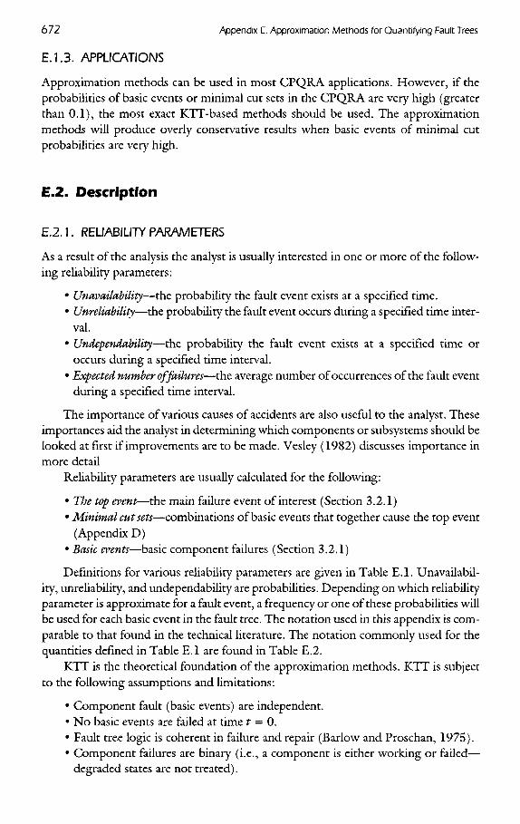
E. 1.3. APPLICATIONS
Approximation methods can be used in most CPQBA applications. However, if theprobabilities of basic events or minimal cut sets in the CPQRA are very high (greaterthan 0.1), the most exact KTT-based methods should be used. The approximationmethods will produce overly conservative results when basic events of minimal cutprobabilities are very high.
E.2. Description
E.2.1. RELIABILITY PARAMETERS
As a result of the analysis the analyst is usually interested in one or more of the follow-ing reliability parameters:
• Unavailability—the probability the fault event exists at a specified time.• Unreliability—the probability the fault event occurs during a specified time inter-
val.• Undependability—the probability the fault event exists at a specified time or
occurs during a specified time interval.• Expected number of failures—the average number of occurrences of the fault event
during a specified time interval.
The importance of various causes of accidents are also useful to the analyst. Theseimportances aid the analyst in determining which components or subsystems should belooked at first if improvements are to be made. Vesley (1982) discusses importance inmore detail
Reliability parameters are usually calculated for the following:
• The top event—the main failure event of interest (Section 3.2.1)• Minimal cutsets—combinations of basic events that together cause the top event
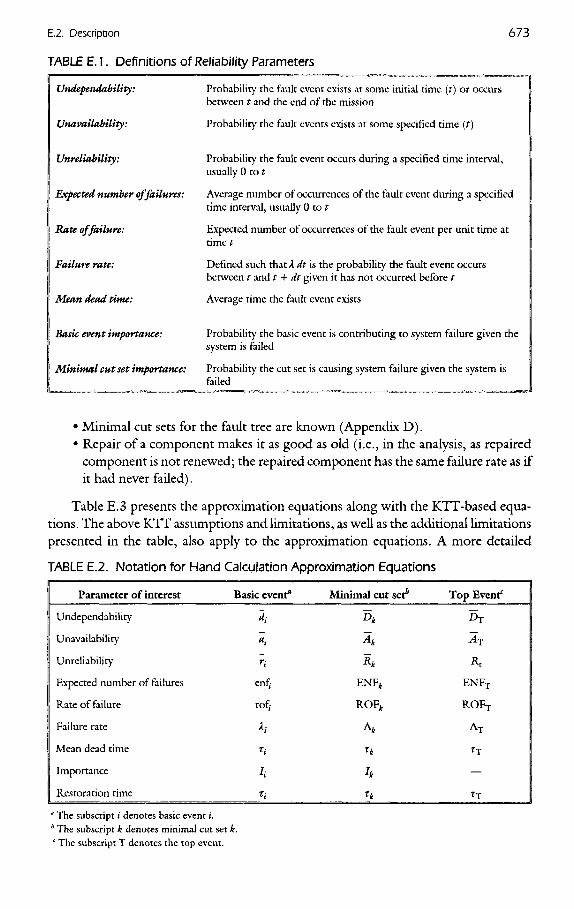
Definitions for various reliability parameters are given in Table E.I. Unavailabil-ity, unreliability, and undependability are probabilities. Depending on which reliabilityparameter is approximate for a fault event, a frequency or one of these probabilities willbe used for each basic event in the fault tree. The notation used in this appendix is com-parable to that found in the technical literature. The notation commonly used for thequantities defined in Table E.I are found in Table E.2.
KTT is the theoretical foundation of the approximation methods. KTT is subjectto the following assumptions and limitations:
• Component fault (basic events) are independent.• No basic events are failed at time £ = O.• Fault tree logic is coherent in failure and repair (Barlow and Proschan, 1975).• Component failures are binary (i.e., a component is either working or failed—
degraded states are not treated).
• Minimal cut sets for the fault tree are known (Appendix D).• Repair of a component makes it as good as old (i.e., in the analysis, as repaired
component is not renewed; the repaired component has the same failure rate as ifit had never failed).
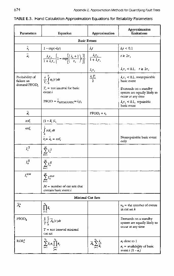
Table E.3 presents the approximation equations along with the KTT-based equa-tions. The above KTT assumptions and limitations, as well as the additional limitationspresented in the table, also apply to the approximation equations. A more detailed
TABLE E.2. Notation for Hand Calculation Approximation Equations
Parameter of interest Basic event* Minimal cut set* Top Event*
Undependability d; D^ Dj
Unavailability ^- Ak Aj
Unreliability r,- Rk Rt
Expected number of failures enf) ENF^ ENF-p
Rate of failure rof- ROF* ROFT
Failure rate A,- A^ AT
Mean dead time r,- Tf1 TJ
Importance Ii Ik —
Restoration time TJ T^ TJ
* The subscript i denotes basic event i.h The subscript k denotes minimal cut set k.0 The subscript T denotes the top event.
Undependability:
Unavailability:
Unreliability:
Expected number of failures:
Rate of failure:
Failure rate:
Mean dead time:
Bask event importance:
Minimal cutset importance:
Probability the fault event exists at some initial time (t) or occursbetween t and the end of the mission
Probability the fault events exists at some specified time (t)
Probability the fault event occurs during a specified time interval,usually O to t
Average number of occurrences of the fault event during a specifiedtime interval, usually Qtot
Expected number of occurrences of the fault event per unit time attime t
Defined such that A dt is the probability the fault event occursbetween t and t + dt given it has not occurred before t
Average time the fault event exists
Probability the basic event is contributing to system failure given thesystem is failed
Probability the cut set is causing system failure given the system isfailed
TABLE E. 1. Definitions of Reliability Parameters
TABLE E. 3. Hand Calculation Approximation Equations for Reliability Parameters
Parameters Equation ApproximationApproximation
limitations
Basic Events
*i
ai
Probability offailure ondemand PFOD,
*i
rot}
enfj
i?
i?
j ENF
1 - exp(-V)
A,T,. L 17 A, + n i l! ,̂a1 cni *< n\
-!-{ wLi O
T; = test interval for basicevent i
PFOD = 0ASYMTOTIC^ tyi
(1-Si)A1.
J rof - dtO
r,-* »,- = enfj-
M
I^k=l
S*k=l
M
^rA-I
M = number of cut sets thatcontain basic event i
VA1T,-
1 + A,T,
A,T,
A, T;2
PFOD, + r,-
A1* < 0.1
t > 2r,
A,T,- < 0.1, f > 2 r {
A,r, < 0.1, nonrepayablebasic event
Demands on a standbysystem are equally likely tooccur at any time
A-T, < 0.1, repairablebasic event
Nonrepayable basic eventonly
Minimal Cut Sets
4T
PFOD*
ROF;
fc^/4(O*^ O
T = test interval minimalcut set
S>,fk»=1 ;=1
;"*
** 1^i
nk = the number of eventsin cut set k
Demands on a standbysystem are equally likely tooccur at any time
#, close to 1
fl, = availability of basicevent i ( 1 - #,-)
nk nk
nk
nk
TABLE E.3. (Continued)
Parameters Equation ApproximationApproximation
limitations
Minimal Cut Sets (continued)
ENF4"
£;Dk
Ak
It
It
j ENFLk
t/ROF^fO
ROF*
A
\AT
*kRT
ENF*ENF7
<ENF*
PFOD4 = Rk
<ROF*
Top Event
AT
*T
ENFT
DT
Ax
TT
N
*ttA = I
N
* E^*A=I
< I]ENF4A = I
N
* EAA = I
N
= 2A*A = I
N = number ofminimum cut sets
.AAT
All basic events arerepairable
* If all the basic events are nonrepairable, then Ak = Rk = ENFt.
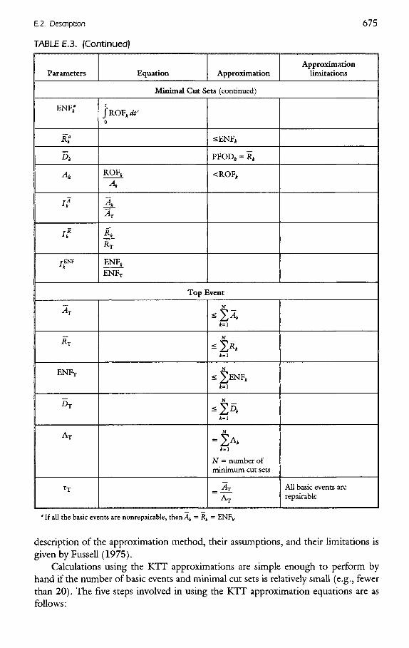
description of the approximation method, their assumptions, and their limitations isgiven by Fussell ( 1975).
Calculations using the KTT approximations are simple enough to perform byhand if the number of basic events and minimal cut sets is relatively small (e.g., fewerthan 20). The five steps involved in using the KTT approximation equations are asfollows:
Step 1: Obtain the basic event failure data.Step 2: Determine the quantity of interest and select the appropriate
equations for calculations.Step 3: Calculate the quantity of interest for each basic event.Step 4: Calculate the quantity of interest for each minimal cut set.Step 5: Calculate the quantity of interest for the top event.
The first step in performing the calculations is to obtain failure data for the basicevents in the fault tree. The failure data include the failure rate (A) and the mean deadtime (T). There are several sources of component failure rates including plant records,operator experience, industry failure data handbooks, and expert opinions (Chapter 5).
The mean dead time is the average time a basic event exists. There are several timesegments counted in the mean dead time. These include the mean time to discover acomponent failure, the mean time to get repairmen and parts, and the mean time toactually repair the component. An additional required input is the mission time, whichis the amount of time a component or system is required to provide its function whendemanded..
The analyst must now decide what reliability parameter is of interest in calculatingand whether to treat an event as repairable or nonrepairable. The appropriate reliabilityparameter may be the frequency of failure (e.g., the expected number of failures peryear), the probability of failure on demand (unavailability), and/or the probability thesystem fails to provide its function during a period of time (unreliability). Since thesereliability parameters have different meanings, and usually different numerical values, itis important that the analyst determine the appropriate parameter of interest for eachtop event.
For example, consider a heating/cooling system for a storage tank that is designedto maintain a monomer within a specified temperature range. Should the system fail inthe heating mode, it could overheat the monomer and potentially trigger a runawaypolymerization reactions. In this case, the appropriate reliability parameter is theexpected frequency of this system failing in the heating mode.
The same heating/cooling system could help prevent a runaway polymerization inthe event the monomer began polymerizing as a result of a different cause. If a poly-merization is occurring, the heating/cooling system may stop the reaction from run-ning away if it responds to the addition heat load by providing adequate cooling for asufficient period of time to stop the reaction. In this case, the appropriate reliabilityparameter is estimated by the sum of the probability of the system failing to start cool-ing when demanded (unavailability) and the probability the system fails to provide ade-quate cooling for a sufficient time (unreliability), if cooling started.
In calculating reliability parameters for any fault tree top event, the analyst mustalso decide for each basic event that appears in the tree whether to "treat" it as repair-able or nonrepairable. In theory every basic event may be repeatable. However, underthe accident conditions modeled in the CPQRA, many basic events should be treatedas nonrepairable. For example, the failure of a standby component may be unknownuntil the component is challenged by an accident at which time it is too late to makerepairs. Failing to treat some basic events as nonrepairable can cause an analyst togreatly underestimate the probability of a component and system failure. On the other
hand, arbitrarily treating all events as nonrepairable can cause the analyst to greatlyoverestimate the probability of a system failure. The following two sections containdetailed descriptions of how to select the appropriate reliability characteristic and howto select repairable or nonrepairable models for basic events.
E.2.2. SELECTING THE APPROPRIATE RELIABILITY PARAMETER
In a CPQBJV, fault trees (Section 3.2.1) may be used to model the causes of an acci-dent-initiating event and/or the failure of safety systems responding to the initiatingevent. If the fault tree top event describes an accident-initiating event, the appropriatereliability parameter to calculate is the failure frequency (expected number of failuresper year).
On the other hand, if the fault tree top event describes a failure of a safety systemresponse, the appropriate reliability parameter is the undependability (D), which isestimated by the sum of the system probability of failure on demand (e.g., an emer-gency scrubber fails to start when needed) and the system unreliability (e.g., anemergency scrubber fails to run for a required period of time). Methods for estimatingthese probabilities are described in Sections 3.1, Chapter 5, and this appendix. In calcu-lating the undependability, the analyst should consider the following factors: (1) thenormal operational status of the safety system and (2) the period of time the safetysystem is required to respond to the emergency. The normal operational status of asafety system is either active or on standby. For active safety systems, the probability offailure on demand (PFOD) is usually small and often assumed to be zero. For standbysafety systems, however, the PFOD is often significant if the system is not tested fre-quently. The period of time the safety system is required to operate, given the accidenthas begun, is the amount of time the system must provide its safety function. As thisperiod of time, often called a mission time, increases, the system unreliability increasesand can become the dominant contribution to the system failure probability.
E.2.3. SELECTING REPAIRABLE OR NONREPAIRABLE MODELSFOR BASIC EVENTS
Basic events appearing in the fault tree models used in a CPQEA represent human andcomponent failures that contribute to a system failure. The failure probabilities of thesebasic events must be estimated by the analyst prior to quantifying the failure frequencyor failure probability of the fault tree top event. In estimating these basic event failureprobabilities, the analyst must determine whether to treat a basic event as repairable ornonrepairable. After selecting a basic event, the analyst should first determine the acci-dent conditions applicable to the basic event as it appears in the fault tree/event treemodel. These conditions may include the environment created by the accident, the lim-itations on repair resources caused by the accident, and the limitations on componentstatus information available. All of these factors will influence the analyst's choice of arepairable or nonrepairable model for the basic event.
Figure E-I outlines the series of steps the analyst should go through to determinewhether to treat a basic event as repairable or nonrepairable. After selecting a basicevent, the analyst should first determine the accident conditions applicable to the basic
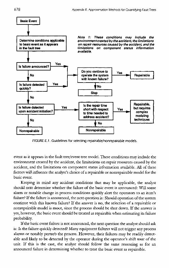
FIGURE E. I. Guidelines for selecting repairable/nonrepairable models.
event as it appears in the fault tree/event tree model. These conditions may include theenvironment created by the accident, the limitations on repair resources caused by theaccident, and the limitations on component status information available. All of thesefactors will influence the analyst's choice of a repairable or nonrepairable model for thebasic event.
Keeping in mind any accident conditions that may be applicable, the analystshould next determine whether the failure of the basic event is announced: Will somealarm or notable change in process conditions quickly alert the operators to an item'sfailure? If the failure is announced, the next question is: Should operation of the systemcontinue with this known failure? If the answer is no, the selection of a repairable ornonrepairable model is moot, since the process should be shut down. If the answer isyes, however, the basic event should be treated as repairable when estimating its failureprobability.
If the basic event failure is not announced, the next question the analyst should askis: Is the failure quickly detected? Many equipment failures will not trigger any processalarms or notably perturb the process. However, their failures may be readily detect-able and likely to be detected by the operator during the operator's shift tour of theunit. If this is the case, the analyst should follow the same reasoning as for anannounced failure in determining whether to treat the basic event as repairable.
Note 1: These conditions may include theenvironment created by the accident the limitationson repair resources caused by the accident and thelimitations on component status informationavailable.
Basic Event
Determine conditions applicableto basic event as it appearsin the fault tree
Is failure announced?Yes
No
Is failure detectedquickly?
Yes
No
Is failure detectedupon accident initiation?
Yes
No
Do you continue tooperate the systemwith known failure?
No
Stop
Is the repair timeshort with respectto time needed toaddress accident?
No
Nonrepairable
Repairable
Repairable,DUt requires
complexmodeling
techniques
Yes
Yes
If the basic event failure is not announced or quickly detected, a final question theanalyst should ask is: Is the failure detected on accident initiation? That is, will thedemand created by an accident initiator disclose whether the basic event is failed? If theanswer is no, the analyst should treat the basic event as nonrepairable. If the answer isyes but there is too little time to repair the basic event under the accident conditionsmodeled, the basic event should again be treated as a nonrepairable event.
If the basic event failure is detected upon accident initiation and sufficient time isavailable to effect repairs under the accident conditions modeled, the basic event maybe viewed as repairable. However, a special complex modeling technique such as delaygate analysis must be used to analyze this type of problem. Discussions of delay gateanalysis methods are beyond the scope of this volume. Risk assessment specialistsshould be consulted for this type of problem. However, it is conservative to treat thebasic event as nonrepairable in these types of problems.
After selecting the appropriate reliability parameter and selecting the repairable ornonrepairable models for basic events, steps 3 through 5 can be completed. The analystsimply has to choose, from Table E.3, the appropriate equation for each step.
E.3. Sample Problems
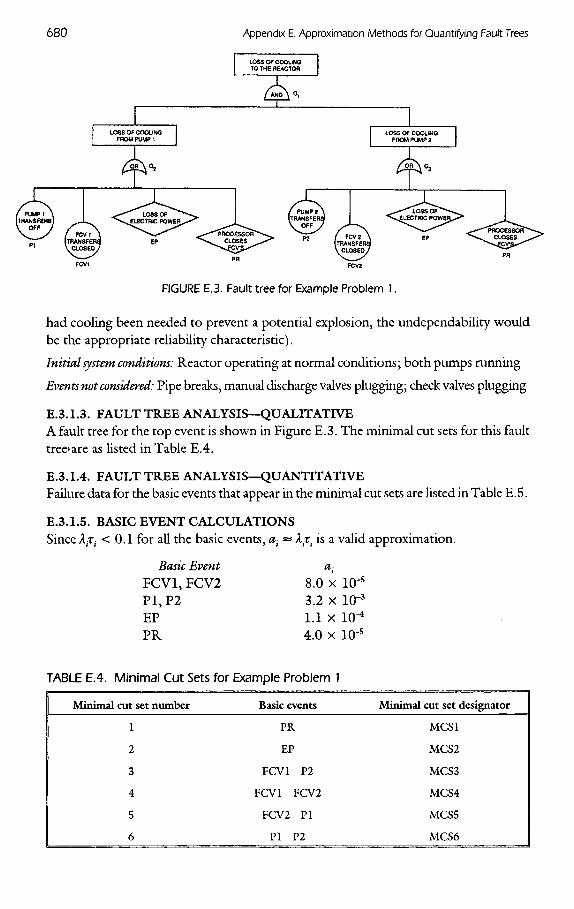
E.3.1. EXAMPLEPROBLEM 1
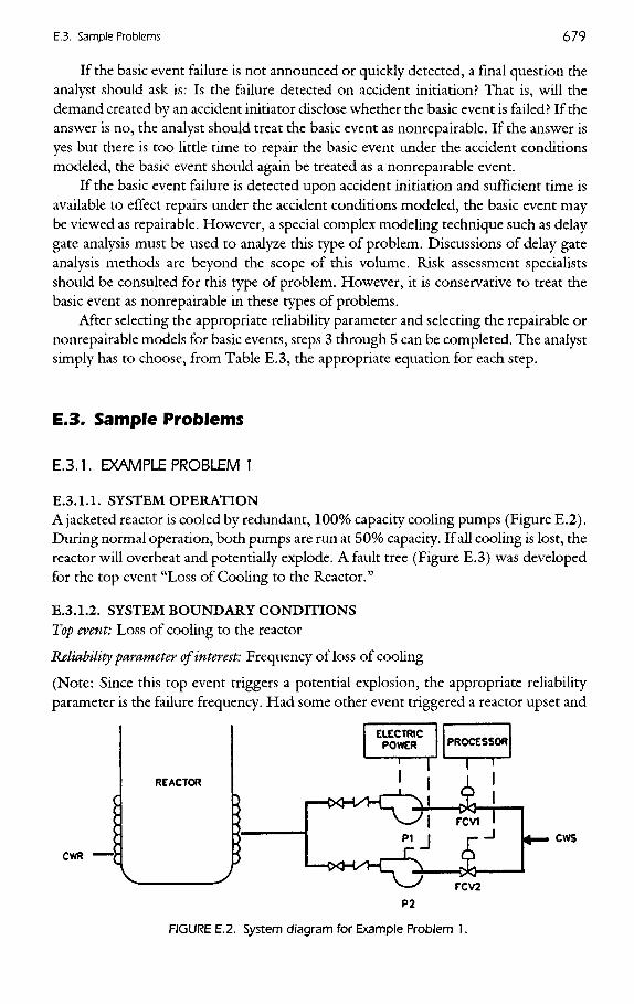
£.3.1.1. SYSTEMOPERATIONA jacketed reactor is cooled by redundant, 100% capacity cooling pumps (Figure E.2).During normal operation, both pumps are run at 50% capacity. If all cooling is lost, thereactor will overheat and potentially explode. A fault tree (Figure E.3) was developedfor the top event "Loss of Cooling to the Reactor."
E.3.1.2. SYSTEMBOUNDARYCONDITIONSTop event: Loss of cooling to the reactor
Reliability parameter of interest: Frequency of loss of cooling
(Note: Since this top event triggers a potential explosion, the appropriate reliabilityparameter is the failure frequency. Had some other event triggered a reactor upset and
FIGURE E.2. System diagram for Example Problem 1.
REACTOR
PROCESSORELECTRICPOWER
FIGURE E.3. Fault tree for Example Problem 1.
had cooling been needed to prevent a potential explosion, the undependability wouldbe the appropriate reliability characteristic).
Initial system conditions: Reactor operating at normal conditions; both pumps running
E.3.1.3. FAULT TREE ANALYSIS—QUALITATIVEA fault tree for the top event is shown in Figure E.3. The minimal cut sets for this faulttree^are as listed in Table E.4.
E.3.1.4. FAULT TREE ANALYSIS—QUANTITATIVEFailure data for the basic events that appear in the minimal cut sets are listed in Table E.5.
E.3.1.5. BASICEVENTCALCULATIONSSince A-T- < 0.1 for all the basic events, ai ~ A-r- is a valid approximation.
Basic Event ai
FCVl, FCV2 8.0 x 10'5
Pl, P2 3.2 x IQ-3
EP 1.1 x 10⁻⁴
PR 4.0 x IQ-5
TABLE E.4. Minimal Cut Sets for Example Problem 1
Minimal cut set number Basic events Minimal cut set designator
LOSS OF COOLINQTO THE REACTOR
LOSSOfCOOLINGFROM PUMP 1 LOSS OF COOLINGFROM PUMP 2
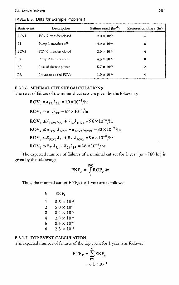
TABLE E.5. Data for Example Problem 1
Basic event Description Failure rate A (hr"1) Restoration time t (hr)
FCVl FCV-I transfers closed 2.0 X 10^5 4
Pl Pump 1 transfers off 4.0 x IQ-4 8
FCV2 FCV-2 transfers closed 2.0 X 10~5 4
P2 Pump 2 transfers off 4.0 X 1(H 8
EP Loss of electric power 5.7 X IQ-5 2
PR Processor closed FCVs 1.0 x IO"5 4
E.3.1.6. MINIMALCUTSETCALCULATIONSThe rates of failure of the minimal cut sets are given by the following:
ROV1 =^PRAP R = 1.0xlO~5/hr
ROV2 = #E PAEp =5.7xl(T5/rir
ROV3 <^FCV1AP2 + 0P2AFCV1 =9.6xlO"8/hr
ROV4 ^FCV1AFCV2 + "FCv2AFcvi =32xl(T9/rir
ROV5 <#FCV2AP1 + #P1AFCV2 =9.6xlO~8/hr
ROV6 < #P1 A P2 + ̂ p2Ap1 =2.6xlO~6/hr
The expected number of failures of a minimal cut set for 1 year (or 8760 hr) isgiven by the following:
8760
ENF fe = / ROF^ dto
Thus, the minimal cut set ENF^s for 1 year are as follows:
k ENF*
1 8.8 x IQ-2
2 5.0 x 10⁻¹
3 8.4 x 10⁻⁴
4 2.8 x 10'5
5 8.4 x 10⁻⁴
6 2.3 x 10⁻²
E.3.1.7. TOPEVENTCALCULATIONThe expected number of failures of the top event for 1 year is as follows:
M
ENF7 =XENF*k=\
= 6.1 XlO'1
E.3.1.8 GATE-BY-BAGE APPROACHUsing the gate-by-gate approach, the top event expected number of failures for 1 yearwould be evaluated as follows:
/(G2) = /(Pl) +/(FCVl) +/(EP) +/(PR)
/(G2) = 4.0 x 10^/hr + 2.0 x lO'Vhr + 5.7 x 10⁻⁵/hr + 1.0 x 10⁻⁵/hr
/(G2) = 4.9 x lO^/hr
/(GS) = /(P2) +/(FCV2) +/(EP) +/(PR)
/(GS) = 4.0 x lO^/hr + 2.0 x 10'5 hr + 5.7 x lO'Vhr + 1.0 x 10'5/hr
/(GS) = 4.9 x lO^/hr
/(Gl) =/(G2) -/(GS) = 2.4 x 10^/hr2
ROFT = 2.4 X lO'Vhr2 (incorrect, units wrong; the gate-by-gatemethod rules have been violated)
8760
ENF7 = J ROFx At = 2.1 X 10~4/hr (incorrect, units wrong)o
Obviously the calculation is in error because two frequencies have been multipliedtogether. According to the gate-by-gate method rules, one of the frequencies must beconverted to a probability. Using 8 hr as the mean downtime for the fault event "Lossof Cooling from Pump 2" (since 8 hr is the largest mean downtime of any basic eventunder this fault event), the probability of this fault event (and GS) is
^GS = /(GS)r G3 =(4.9xlO"4/hr)(8hr)=3.9xlO"3
The top event expected number of failures in 1 year would be calculated as follows:
ROFx=/(Gl) = /(02)^3
ROFx = (4.9 x 10⁻⁴/hr)(3.9 x 10*) = 1.9 x 10"6 (incorrect)8760
ENF7 = J ROFT dt = 1.7 x lO'Vrir (incorrect)o
The calculated expected number of failures is incorrect due to the presence of basicevents EP and PR on two legs of the AND gate Gl. Since these faults can contribute tothe event only once, the second contribution should be eliminated from the calcula-tions. If the analyst is careful, he can catch these repeated events and prevent them frombeing used twice. However, this can be difficult if a repeated event is buried in layers offault tree logic. The minimal cut set approach handles this problem implicitly andwould be the preferred method in this case.
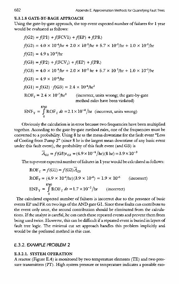
E.3.2. EXAMPLE PROBLEM 2
E.3.2.1. SYSTEMOPERATIONA reactor (Figure E.4) is monitored by two temperature elements (TE) and two pres-sure transmitters (PT). High system pressure or temperature indicates a possible exo-
FIGURE E.4. System diagram for Example Problem 2.
thermic reaction in progress. The processor provides a shutdown signal if it receives ahigh signal from either the TEs or the PTs. The reaction pressure and temperature arecontinuously monitored. The processor is tested once every shift (8 hr). If the proces-sor (combination of output card and CPU) is found failed, the reaction is shut downwhile the processor is repaired.
E.3.2.2. SYSTEM BOUNDARY CONDITIONSTop Event: Loss of capability to shut down
Reliability parameter if interest: Probability the safety system fails to shut down the reac-tor when required (PFOD)
Initial system condition: Reactor is running at normal process conditions.(Note: The concern here is not how often the system fails, but if it is failed when
you need it, i.e., when a process upset occurs. Thus, we must calculate the systemundependability. However, since the system completes its work just milliseconds afterit starts, the undependability in this case is just the PFOD).
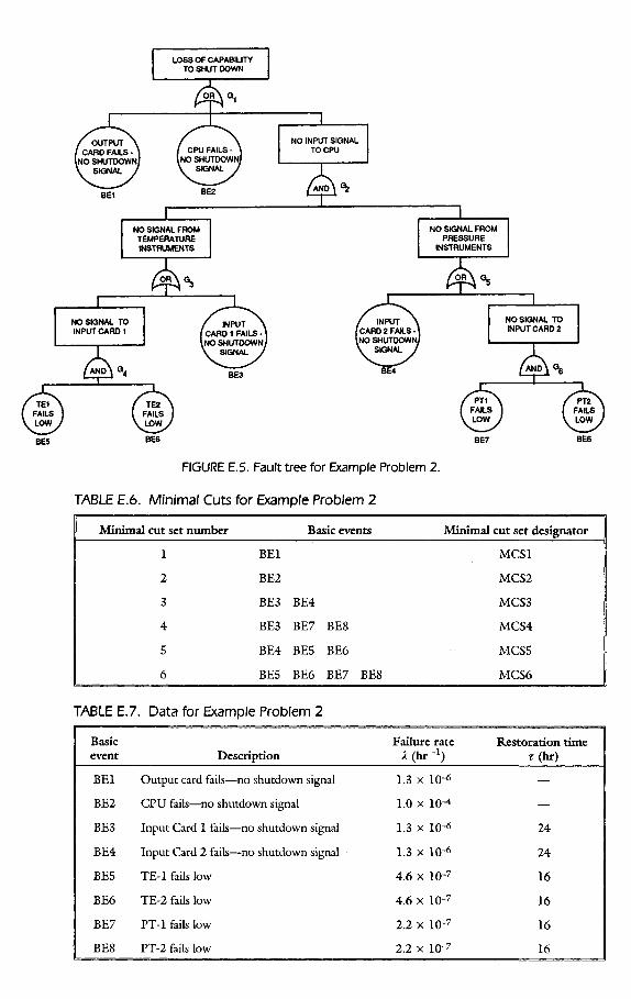
E.3.2. FAULT TREE ANALYSIS—QUALITATIVEA fault tree for the top event is shown in Figure E.5. The minimal cut sets for this faulttree are listed in Table E.6.
E.3.2.4. FAULT TREE ANALYSIS-QUANTITATIVEFailure data for the basic events that appear in the minimal cut sets are listed in Table E.7.
E.3.2.5 BASIC EVENT CALCULATIONSFor each event i} A1- ri < 0.1. The analyst is interested in the average unavailability over ayear, so t >2ri. Therefore, the approximation a. s A .r. is a valid one. Since the failures
REACTORSHUTDOWN
SIGNAL
OUTPUTCARD
INPUTCARD 1
INPUTCARD 2
FIGURE E.5. Fault tree for Example Problem 2.
TABLE E.6. Minimal Cuts for Example Problem 2
Minimal cut set number Basic events Minimal cut set designator
1 BEl MCSl
2 BE2 MCS2
3 BE3 BE4 MCS3
4 BE3 BE7 BE8 MCS4
5 BE4 BE5 BE6 MCS5
6 BE5 BE6 BE7 BE8 MCS6
TABLE E.7. Data for Example Problem 2
Basic Failure rate Restoration timeevent Description X (hr ~l) r (hr)
BEl Output card fails—no shutdown signal 1.3 X 10"6 —
BE2 CPU fails—no shutdown signal 1.Ox-I(H —
BE3 Input Card 1 fails—no shutdown signal 1.3 X IQ-6 24
BE4 Input Card 2 fails—no shutdown signal 1.3 X IO"6 24
BE5 TE-I fails low 4.6 x 10~7 16
BE6 TE-2 fails low 4.6 X 10~7 16
BE7 PT-I fails low 2.2 X 10~7 16
BE8 PT-2 fails low 2.2 X 10~7 16
LOSS OF CAPABILITYTO SHUT DOWN
NO INPUT SIGNALTOCPU/ OUTPUT \
CARD FAILS - ^NO SHUTDOWN,<. SIGNAL /
CPUFAILS- 1NO SHUTDOWNj^ SIGNAL J
NO SIGNAL FROMTEMPERATUREINSTRUMENTS
NOSIGNAL TOINPUT CARD 1 r INPUT >
CARD 1 FAILS -NOSHUTDOWNV SIGNAL >
( INPUT \CARD2 FAILS-'NO SHUTDOWN-^ SIGNAL /
NO SIGNAL FROMPRESSURE
INSTRUMENTS
NO SIGNAL TOINPUT CARD 2
PT2FAILSLOW
PT1FAILSLOW
TE2FAILS
. LOWTE1
FAILSLOW
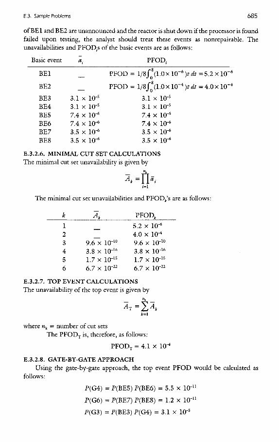
of BEl and BE2 are unannounced and the reactor is shut down if the processor is foundfailed upon testing, the analyst should treat these events as nonrepairable. Theunavailabilities and PFOD-s of the basic events are as follows:
Basic event ^. PFOD,
BEl _ PFOD = 1/8/^(1.0x 10"6X^f= 5.2 XlO"6
BE2 _ PFOD = l/8/o8(1.0xlO"4X^ = 4.0xlO"4
BE3 3.1 x 1(TS 3.1 x IQ-5
BE4 3.1 x IQ-5 3.1 x 1(T5
BE5 7.4 x IQ-6 7.4 x 1(T6
BE6 7.4 x ID"6 7.4 x ICT6
BE7 3.5 x IQ-6 3.5 x 1(T6
BE8 3.5 x IQ-6 3.5 x 1(T6
E.3.2.6. MINIMAL CUT SET CALCULATIONSThe minimal cut set unavailability is given by
A=fk;=1
The minimal cut set unavailabilities and PFOD^s are as follows:
* A± PFOD,
1 _ 5.2 x ID"6
2 _ 4.0 x 1(T1
3 9.6 x ID"10 9.6 x 1(T10
4 3.8 x IQ-16 3.8 x 1(T16
5 1.7 x ICT15 1.7 x IQ-15
6 6.7 x IQ-22 6.7 x 1(T22
E.3.2.7. TOP EVENT CALCULATIONSThe unavailability of the top event is given by
^T=XA6=1
where nk = number of cut setsThe PFODx is, therefore, as follows:
PFOD7 = 4.1 x 1(T*
E.3.2.8. GATE-BY-GATE APPROACHUsing the gate-by-gate approach, the top event PFOD would be calculated as
follows:
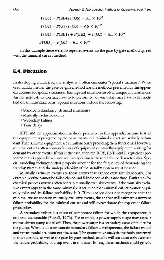
P(G4) = P(BES) P(BE6) = 5.5 x 1(T11
P(G6) = P(BE7) P(BES) = 1.2 x 1(T11
P(GS) =P(BE3)P(G4) = 3.1 x 1(T5
P(GS) = P(BE4) P(G6) = 3.1 x 1(T5
P(G2) = P(GS) P(GS) = 9.6 x 1(T10
P(Gl) = P(BEl) + P(BE2) + P(G2) = 4.1 x 10"4
PFODx = P(Gl) = 4.1 x IQ-4
In this example there were no repeated events, so the gate-by-gate method agreedwith the minimal cut set method.
E.4. Discussion
In developing a fault tree, the analyst will often encounter "special situations." Whenused blindly neither the gate-by-gate method nor the methods presented in this appen-dix account for special situations. Each special situation involves unique circumstances.An alternate calculation may have to be performed, or some data may have to be modi-fied on an individual basis. Special situations include the following:
KIT and the approximation methods presented in this appendix assume that allthe equipment represented by the basic events in a minimal cut set are actively redun-dant That is, all the equipment are simultaneously providing their functions. However,minimal cut sets often contain failures of equipment on standby-equipment waiting fordemand by other events. If this is the case, then the ROF, ENF, and R equations pre-sented in this appendix will not accurately estimate these reliability characteristics. Spe-cial modeling techniques that properly account for the frequency of demands on thestandby system and the undependability of the standby system must be used.
Mutually exclusive events are those events that cannot exist simultaneously. Forexample, a valve cannot be failed closed and failed open at the same time. Fault trees forchemical process systems often contain mutually exclusive events. If the mutually exclu-sive events appear in the same minimal cut set, then that minimal cut set cannot physi-cally exist and its failure probability is O. If the analyst does not recognize that theminimal cut set contains mutually exclusive events, the analyst will estimate a nonzerofailure probability for the minimal cut set and will overestimate the top event failureprobability.
A secondary failure is a cause of component failure for which the component, isnot held accountable (Fussell, 1976). For example, a power supply surge may cause amotor-driven pump to fail off. Thus, the power surge is a secondary cause of failure forthe pump. When fault trees contain secondary failure developments, the failure modeland repair model are often not the same. The quantitative analysis methods presentedin this appendix, as well as the gate-by-gate method, usually will not accurately estimatethe failure probability of a top event in this case. In fact, these methods could grossly
underestimate the failure probability. Special modeling techniques must be used in thiscase.
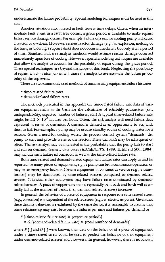
Another situation encountered in fault trees is time delays. Often, when an inter-mediate fault event in a fault tree occurs, a grace period is available to make repairsbefore serious damage occurs. For example, failure of a reactor cooling pump will causea reactor to overheat. However, serious reactor damage (e.g., an explosion, melting ofthe liner, or blowing a rupture disk) does not occur immediately but only after a periodof time. Standard fault tree analysis methods would assume reactor damage occurredimmediately upon loss of cooling. However, special modeling techniques are availablethat allow the analyst to account for the possibility of repair during this grace period.These special techniques are beyond the scope of this book. Neglecting the possibilityof repair, which is often done, will cause the analyst to overestimate the failure proba-bility of the top event.
There are two commonly used methods of summarizing equipment failure histories:
The methods presented in this appendix use time-related failure rate data of vari-ous equipment items as the basis for the calculation of reliability parameters (i.e.,undependability, expected number of failures, etc.) A typical time-related failure ratemight be 1.2 X 10~3 failures per hour. Often, the risk analyst will need failure dataexpressed in terms of demands. A demand is defined as an opportunity to act, and,thus, to fail. For example, a pump may be used as standby source of cooling water for areactor. Given a need for cooling water, the process control system "demands" thepump to start and provide water to the reactor. These demands may be infrequent oroften. The risk analyst may be interested in the probability that the pump fails to startand run on demand. Generic data bases (AIChE/CPPS, 1989; IEEE std 500, 1984)may include such failure information as well as the time-related failure rate.
Both time-related and demand-related equipment failure rates can apply to and bereported for many pieces of equipment, e.g., a pump can be in continuous operation ormay be an emergency backup. Certain equipment in continuous service (e.g., a trans-former) may be dominated by time-related stresses compared to demand-relatedstresses. Likewise, other equipment may have failure rates dominated by demand-related stresses. A piece of copper wire that is repeatedly bent back and forth will even-tually fail as the number of bends (i.e., demand related stresses) increases.
In general, the behavior of a piece of equipment in response to a time related stress(e.g., corrosion) is independent of the related stress (e.g., an electric impulse). Given thatthese distinct behaviors are exhibited by the same device, it is reasonable to assume thatsome relationship may exist between the failures per time and failures per demand or
F [(time-related failure rate) X (exposure period)]oc G [(demand-related failure rate) X (total number of demands)]
where F [ ] and G [ ] were known, then data on the behavior of a piece of equipmentunder a time-related stress could be used to predict the behavior of that equipmentunder demand-related stresses and vice-versa. In general, however, there is no known
mathematical relationship between these behaviors based on fundamental reliabilityengineering principles. The availability of a mathematical relationship that defines F [ ]and G [ ] is very uncommon. F [ ] and G [ ] would be very unique to a specific piece ofequipment, its operating and maintenance history, its testing, the accounting systemused to assign and record failures, its failure history, and so on.
In most cases, the failure history available for a CPQRA will summarize the experi-ence of many equipment items. Those items in continuous service will be used to com-pute the time-related equipment failure rate. Those items in a demand type of servicewill be used to compute the demand-related equipment failure rate. The PERD Guide-lines (AIChE/CCPS, 1989) offers further discussion on some of the complicating fac-tors that influence the mathematical relationship proposed in Eq. (5.5.8), and proposeshow both kinds of failure rate data should be handled.
E.5. References
AICHE/CCPS (1989). Guidelines for Process Equipment Reliability Data. Center for ChemicalProcess Safety, American Institute for Chemical Engineers, New York.
Barlow, R. E. and Proschan, F. (1975). Statistical Theory of Reliability and Life Testing ProbabilityModels. Holt, Reinhart & Winston, New York (ISBN 0-9606764-0-6).
Fussell, J. B. (1976). "Fault Tree Analysis-Concepts and Techniques." Generic Techniques in Sys-tems Reliability Assessment. Proceedings of the NATO Advanced Study Institute on Generic Tech-niques in Systems Reliability Assessment, University of Liverpool, United Kingdom, July 17-18, 1973 (EJ. Henley and J. W. Glynn, eds.), pp. 133-162. Noordhoff, Keyden.
Fussell, J. B. (1975). "How to Hand-Calculate System Reliability and Safety Characteristics."IEEE Transactions on Reliability R-24(3), 169-174.
IEEE std 500 (1984). Guide to the Collection and Presentation of Electrical., Electronic^ Sensing Com-ponent, and Mechanical Equipment Reliability Data for Nuclear Power Generating Stations.IEEE Std 500-1984, Institute of Electrical and Electronic Engineers, New York. (IEEE Cat.no. SH 10728.)
Vesley, W. E., (1970). "A Time Dependent Methodology for Fault Tree Evaluation." NuclearEngineering and Design 13, 377-360, North-Holland, Amsterdam, AUGUST.
Vesley W. E. etal. (1983) Measure of Risk Importance and Their Applications. NUREG/CR-3385,Battelle Columbus Laboratories, Columbus, OH, July.


![Index [ftp.feq.ufu.br]ftp.feq.ufu.br/Luis_Claudio/Segurança/Safety/Double/fire_handbook... · Backdraft Explosion 174 Barium 216 Barium Carbonate 300 Barium Chlorate 300 Barium Nitrate](https://static.documents.pub/doc/80x56/5ea2585052451660ed3ed304/index-ftpfequfubrftpfequfubrluisclaudioseguranasafetydoublefirehandbook.jpg)
![Index [ftp.feq.ufu.br]ftp.feq.ufu.br/.../Double/fire_handbook/14298_indx.pdf · BLEVE (Boiling Liquid Expanding Vapor Explosion) 224 Block off Operations 197 Boiler Compound, Liquid](https://static.documents.pub/doc/80x56/5ea2589dad656856d47e9db5/index-ftpfequfubrftpfequfubrdoublefirehandbook14298indxpdf-bleve.jpg)


![Index [ftp.feq.ufu.br]ftp.feq.ufu.br/Luis_Claudio/Books/E-Books... · Aeration-agitation 20, 46 Aeration-agitation bioreactor 58, 62 Aerobic fermentation 3, 18 1 Aerobic metabolic](https://static.documents.pub/doc/80x56/5ecd4084c5979741945851bb/index-ftpfequfubrftpfequfubrluisclaudiobookse-books-aeration-agitation.jpg)