Appendix N—Grand Inversion Implementation and Testing

Appendix N—Grand Inversion Implementation and Testing

By Morgan T. Page1, Edward H. Field1, Kevin R. Milner2, and Peter M. Powers1

Abstract We present results from an inversion-based methodology developed for the third Uniform

California Earthquake Rupture Forecast (UCERF3) that simultaneously satisfies available slip-rate, paleoseismic event-rate, and magnitude-distribution constraints. Using a parallel simulated-annealing algorithm, we solve for the long-term rates of all ruptures that extend through the seismogenic thickness on major mapped faults in California. In this system-level approach, rupture rates, rather than being prescribed by experts as in past models, are derived directly from data. The inversion methodology enables the relaxation of fault segmentation and allows for the incorporation of multi-fault ruptures, which are needed to remove magnitude-distribution misfits that were present in the previous model, UCERF2. In addition to UCERF3 model results, we present verification of the inversion methodology, including sensitivity tests, convergence metrics, and a synthetic test.

Introduction The evaluation of earthquake rupture forecasts in California dates back to the original

Working Group on California Earthquake Probabilities (WGCEP; 1988), which considered the probabilities of future earthquakes on different segments of the San Andreas Fault. The most recent California model, UCERF2 (Working Group on California Earthquake Probabilities, 2007), used expert opinion to determine the rates of ruptures on many of the major faults. This expert opinion framework is not compatible with the incorporation of significant numbers of multi-fault ruptures on a large, complex fault system. Furthermore, in UCERF2 methodology, there was no way to simultaneously constrain that the model fit both observed paleoseismic event rates and fault slip rates. These limitations were recognized by the leaders of the UCERF2 effort; however it was not possible to address them at the time given the available tools. The 3rd Uniform California Earthquake Rupture Forecast (UCERF3) uses a more algorithmic approach to consider possible future earthquakes on a much larger number of faults. The primary goals in the development of UCERF3, described in this study and in the main text to this report), have been to consider more potential sources (faults), relax segmentation, include multi-fault ruptures, and adhere to the observed regional magnitude distribution. These goals motivated the development of an inversion approach in UCERF3. This inversion, which has become colloquially known as the “grand inversion,” is described in detail in this study. 1 U.S. Geological Survey. 2 University of Southern California.

Appendix N of Uniform California Earthquake Rupture Forecast, Version 3 (UCERF3)

2

The purpose of the grand inversion is to solve for the long-term rate of all possible ruptures on the major faults in California. The rates of these ruptures are constrained by fault slip rates, paleoseismic event rates and average slips, magnitude-frequency distributions (MFDs) observed in seismicity (and adjusted to account for background seismicity), as well as other a priori and smoothing constraints described below.

We use an inversion methodology based on a method proposed by Andrews and Schwerer (2000) and further developed by Field and Page (2011). Because of the size of the numerical problem, we use a simulated annealing algorithm (Kirkpatrick and others, 1983) to invert the ruptures rates. The simulated annealing method also has the advantage that it can give multiple solutions that satisfy the data. This allows us to more fully explore the epistemic uncertainty present in the problem. Below we describe (1) the constraints used in the inversion, (2) the simulated annealing algorithm that solves the inverse problem, (3) testing of the inversion methodology, and (4) final UCERF3 modeling results.

Setting Up the Inversion: Data and Constraints Following earlier UCERF efforts, UCERF3 uses a logic-tree approach to take alternative

models and parameters into account (main text, this report). The full UCERF3 logic tree is shown in figure N1. The UCERF3 reference branch is shown in bold. The reference branch is not intended to represent the preferred branch, but rather provides a reference with which to compare models using other branches on the logic tree.

The fault models listed in the logic tree define the geometries of fault sections (appendix A, this report). Fault sections include single faults such as Puente Hills; larger faults are divided into several sections (for example, San Andreas Mojave North). These fault sections are divided into subsections that are approximately 7 km long on average (for more details, see main text of this report). These subsections are for numerical tractability and do not have geologic meaning.

The inversion methodology solves for the rates of ruptures that are consistent with the data and constraints described below. Some of these constraints differ depending on the inversion model branch; here we describe and present the Characteristic branch solution, which is constrained to have fault MFDs that are as close to UCERF2 MFDs as possible, because UCERF2 assumed a characteristic magnitude distribution on faults (Wesnousky and others, 1983; Schwartz and Coppersmith, 1984). The inversion can also be used to solve for rates consistent with Gutenberg-Richter (GR) MFDs (Gutenberg and Richter, 1944), or the on-fault MFDs can be unconstrained and allowed to be whatever best satisfies the other constraints. Here we describe only the Characteristic branch solution and setup, because this branch is closest to what was done in the previous UCERF2 model, and it more easily satisfies historical seismicity rates than the GR branch (see the main text of this report for more details).

The Characteristic branch is designed to be as similar as possible to the UCERF2 rupture rates, while simultaneously satisfying slip rates and paleoseismic data, allowing multi-fault ruptures, and eliminating the magnitude distribution “bulge” (overprediction relative to seismicity rates) that existed in the UCERF2 model.


3

Figure N1. Diagram of the UCERF3 logic tree and branch weights. The reference branch is shown in bold.

Inversion Constraints Slip Rates

The average slip in each rupture that includes a given fault subsection, multiplied by the rate of that rupture, must sum to the long-term slip rate for that subsection, as given by the deformation model (appendixes B and C, this report). The slip rates used in this constraint have been reduced from the slip rates specified in the deformation models to account for subseismogenic-thickness ruptures and aseismicity (see the main text of this report for more details). This constraint is applied to each fault subsection in both normalized and unnormalized form. For the normalized constraint, each slip rate constraint is normalized by the target slip rate


4

(so that misfit is proportional to the fractional difference, rather than the absolute difference, between the model slip rates and the target slip rates), with the exception of slip rates below 0.1 mm/yr. This prevents some extremely low slip rates from dominating the misfit. Including both normalized and unnormalized forms of this constraint means we are minimizing both the ratio and the difference between the target and model slip rates; this approach represents a balance between better fitting slip rates on fast faults such as the San Andreas versus smaller slip rates on slower, secondary faults. These constraints can be written as

�𝐷𝑠𝑟

𝑅

𝑟=1

𝑓𝑟 = 𝑣𝑠 and �𝐷𝑠𝑟𝑣𝑠′

𝑅

𝑟=1

𝑓𝑟 =𝑣𝑠𝑣𝑠′

,

where 𝑣𝑠′ = max(𝑣𝑠, 0.1 mm/yr), 𝑣𝑠 is the 𝑠𝑡ℎ subsection slip rate, 𝑓𝑟 is the long-term rate of the 𝑟𝑡ℎ rupture, and 𝐷𝑠𝑟 is the average slip on the 𝑠𝑡ℎ subsection in the 𝑟𝑡ℎ rupture. Depending on the logic-tree branch, 𝐷𝑠𝑟 is either a uniform distribution along strike or a tapered distribution (appendix F, this report).

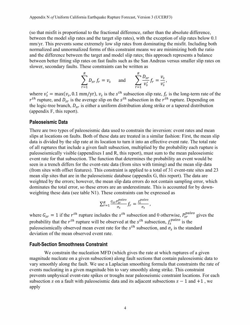
Paleoseismic Data There are two types of paleoseismic data used to constrain the inversion: event rates and mean slips at locations on faults. Both of these data are treated in a similar fashion: First, the mean slip data is divided by the slip rate at its location to turn it into an effective event rate. The total rate of all ruptures that include a given fault subsection, multiplied by the probability each rupture is paleoseismically visible (appendixes I and R, this report), must sum to the mean paleoseismic event rate for that subsection. The function that determines the probability an event would be seen in a trench differs for the event-rate data (from sites with timing) and the mean slip data (from sites with offset features). This constraint is applied to a total of 31 event-rate sites and 23 mean slip sites that are in the paleoseismic database (appendix G, this report). The data are weighted by the errors; however, the mean slip data errors do not contain sampling error, which dominates the total error, so these errors are an underestimate. This is accounted for by down-weighting these data (see table N1). These constraints can be expressed as

∑ 𝐺𝑠𝑟𝑃𝑠𝑟𝑝𝑎𝑙𝑒𝑜

𝜎𝑠𝑓𝑟𝑅

𝑟=1 = 𝑓𝑠𝑝𝑎𝑙𝑒𝑜

𝜎𝑠 ,

where 𝐺𝑠𝑟 = 1 if the 𝑟𝑡ℎ rupture includes the 𝑠𝑡ℎ subsection and 0 otherwise, 𝑃𝑠𝑟𝑝𝑎𝑙𝑒𝑜 gives the

probability that the 𝑟𝑡ℎ rupture will be observed at the 𝑠𝑡ℎ subsection, 𝑓𝑠𝑝𝑎𝑙𝑒𝑜 is the

paleoseismically observed mean event rate for the 𝑠𝑡ℎ subsection, and 𝜎𝑠 is the standard deviation of the mean observed event rate.

Fault-Section Smoothness Constraint We constrain the nucleation MFD (which gives the rate at which ruptures of a given

magnitude nucleate on a given subsection) along fault sections that contain paleoseismic data to vary smoothly along the fault. We use a Laplacian smoothing formula that constraints the rate of events nucleating in a given magnitude bin to vary smoothly along strike. This constraint prevents unphysical event-rate spikes or troughs near paleoseismic constraint locations. For each subsection 𝑠 on a fault with paleoseismic data and its adjacent subsections 𝑠 − 1 and +1 , we apply


5

(𝑅𝑠𝑚 − 𝑅𝑠−1𝑚 ) + (𝑅𝑠𝑚 − 𝑅𝑠+1𝑚 ) = 0,

where 𝑅𝑠𝑚 is the nucleation rate of events in the 𝑚𝑡ℎ magnitude bin on the 𝑠𝑡ℎ subsection. At fault edges (where a subsection 𝑠 has one adjacent subsection 𝑠 − 1), this constraint becomes

𝑅𝑠𝑚 − 𝑅𝑠−1𝑚 = 0.

Parkfield Rupture-Rate Constraint We constrain the total rate of Parkfield M~6 ruptures, which have been observed to be

quasi-periodic (Bakun and Lindh, 1985), to match the observed mean recurrence interval of 25 years. There are six “Parkfield earthquakes” included in the constraint, one rupture that includes all 8 Parkfield subsections, the two 7-subsection long ruptures, and the three 6-subsection long ruptures in the Parkfield section of the San Andreas Fault (SAF). We choose a range of ruptures, rather than the single Parkfield-section-long rupture, because of evidence that past M~6 earthquakes in Parkfield have ruptured slightly different areas of the fault (Custódio and Archuleta, 2007). The Parkfield earthquakes are not included in the MFD constraints discussed below, because the target on-fault magnitude distribution for some branches does not have a high enough rate at M6 to accommodate the Parkfield constraint. Tuning of the creep-based moment-rate reduction in the Parkfield section is required to obtain the correct approximate magnitude for the Parkfield earthquakes; this is discussed below in the section on “Parkfield and Creeping Section Moment-Rate Reduction Tuning.” The Parkfield constraint is the only type of a priori event-rate constraint we apply in UCERF3. These types of constraints are simply written as 𝑓𝑟 = 𝑓𝑟

𝑎−𝑝𝑟𝑖𝑜𝑟𝑖, where 𝑓𝑟𝑎−𝑝𝑟𝑖𝑜𝑟𝑖 is the a priori rate of the 𝑟𝑡ℎ rupture.

Nonnegativity Constraint Rupture rates cannot be negative. This is a hard constraint that is not included in the

system of equations but is strictly enforced in the simulated annealing algorithm, which does not search any solution space that contains negative rates. In UCERF3 we impose a stricter constraint than nonnegativity; namely, a minimum rate for each rupture (“water-level”), which can be transformed into an equivalent problem with a simple nonnegativity constraint, as discussed below.

Fault Section MFD Constraint This constraint is applied to Characteristic branch solutions and constrains the MFDs on

fault subsections to be close to the characteristic MFDs used in UCERF2. UCERF2 contained Type-A faults for which ruptures linking different fault sections (for example, different sections of the San Andreas) were allowed; for these faults, we constrain the MFD to be close to the MFD that was used in UCERF2. For the remaining faults (both faults that were Type-B faults in UCERF2 and newly added faults that were not in UCERF2), we construct an MFD consistent with UCERF2 MFD-methodology (see the main text of this report for more details). This constraint can be written as

�𝑀𝑠𝑟𝑚

𝑅𝑠𝑚

𝑅

𝑟=1

𝑓𝑟 = 1 , for all 𝑅𝑠𝑚 > 0,


6

where 𝑀𝑠𝑟𝑚 is the fraction of the 𝑟𝑡ℎ rupture of events in the 𝑚𝑡ℎ magnitude bin on the 𝑠𝑡ℎ

subsection. Rupture rates for magnitude bins where 𝑅𝑠𝑚 = 0 are also minimized.

Regional Magnitude Distribution Constraint The on-fault target magnitude distribution for the Characteristic branch is a trilinear

model as shown in figure N2. Above the maximum magnitude for off-fault seismicity, the on-fault MFD equals the total (on-fault plus off-fault) magnitude distribution (total seismicity rates are estimated from historical seismicity, see appendix L, this report).

Figure N2. Schematic graph of magnitude-frequency distributions for the UCERF3 reference branch. The total target magnitude frequency distribution (found from seismicity, see appendix L, this report) is shown in black. It is reduced to account for off-fault earthquakes and ruptures whose lengths are less than the subseismogenic thickness; this gives the supraseismogenic on-fault target, shown in blue, which is used to constrain the regional MFD given by the inversion solution.

Below the maximum off-fault magnitude, the on-fault MFD transitions to a lower b-value, and then transitions again back to a b-value of 1.0 (matching historical seismicity) at about M6.25 (this is the average minimum magnitude for the supraseismogenic-thickness ruptures, the exact value of which is branch-dependent). The rate of M≥5 events for the on-fault MFD is set from historical seismicity that is inside our fault polygons (as described in the main text of this report). Thus the entire on-fault MFD is uniquely determined by the maximum off-fault magnitude, the average minimum magnitude for the on-fault, supraseismogenic-thickness ruptures, historical seismicity rates, and the fraction of seismicity that is considered “on-fault” (within our fault polygons).

The inversion solves only for rates of earthquakes that are as long in the along-strike direction as the (local) seismogenic thickness, so the on-fault MFD is then reduced at low magnitudes by the rate of subseismogenic ruptures on each fault section. This gives the


7

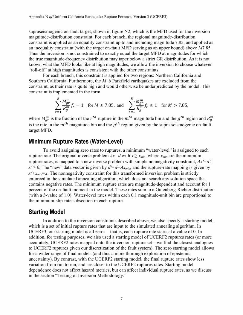
supraseismogenic on-fault target, shown in figure N2, which is the MFD used for the inversion magnitude-distribution constraint. For each branch, the regional magnitude-distribution constraint is applied as an equality constraint up to and including magnitude 7.85, and applied as an inequality constraint (with the target on-fault MFD serving as an upper bound) above M7.85. Thus the inversion is not constrained to exactly equal the target MFD at magnitudes for which the true magnitude-frequency distribution may taper below a strict GR distribution. As it is not known what the MFD looks like at high magnitudes, we allow the inversion to choose whatever “roll-off” at high magnitudes is consistent with the other constraints.

For each branch, this constraint is applied for two regions: Northern California and Southern California. Furthermore, the M~6 Parkfield earthquakes are excluded from the constraint, as their rate is quite high and would otherwise be underpredicted by the model. This constraint is implemented in the form

�𝑀𝑔𝑟𝑚

𝑅𝑔𝑚

𝑅

𝑟=1

𝑓𝑟 = 1 for 𝑀 ≤ 7.85, and �𝑀𝑔𝑟𝑚

𝑅𝑔𝑚

𝑅

𝑟=1

𝑓𝑟 ≤ 1 for 𝑀 > 7.85,

where 𝑀𝑔𝑟𝑚 is the fraction of the 𝑟𝑡ℎ rupture in the 𝑚𝑡ℎ magnitude bin and the 𝑔𝑡ℎ region and 𝑅𝑔𝑚

is the rate in the 𝑚𝑡ℎ magnitude bin and the 𝑔𝑡ℎ region given by the supra-seismogenic on-fault target MFD.

Minimum Rupture Rates (Water-Level) To avoid assigning zero rates to ruptures, a minimum “water-level” is assigned to each

rupture rate. The original inverse problem Ax=d with x ≥ xmin, where xmin are the minimum rupture rates, is mapped to a new inverse problem with simple nonnegativity constraint, Ax′=d′, x′ ≥ 0. The “new” data vector is given by d′=d−Axmin, and the rupture-rate mapping is given by x′+xmin=x. The nonnegativity constraint for this transformed inversion problem is strictly enforced in the simulated annealing algorithm, which does not search any solution space that contains negative rates. The minimum rupture rates are magnitude-dependent and account for 1 percent of the on-fault moment in the model. These rates sum to a Gutenberg-Richter distribution (with a b-value of 1.0). Water-level rates within each 0.1 magnitude-unit bin are proportional to the minimum-slip-rate subsection in each rupture.

Starting Model In addition to the inversion constraints described above, we also specify a starting model,

which is a set of initial rupture rates that are input to the simulated annealing algorithm. In UCERF3, our starting model is all zeros—that is, each rupture rate starts at a value of 0. In addition, for testing purposes, we also used a starting model of UCERF2 ruptures rates (or more accurately, UCERF2 rates mapped onto the inversion rupture set—we find the closest analogues to UCERF2 ruptures given our discretization of the fault system). The zero starting model allows for a wider range of final models (and thus a more thorough exploration of epistemic uncertainty). By contrast, with the UCERF2 starting model, the final rupture rates show less variation from run to run, and are closer to the UCERF2 ruptures rates. Starting model dependence does not affect hazard metrics, but can affect individual rupture rates, as we discuss in the section “Testing of Inversion Methodology.”


8

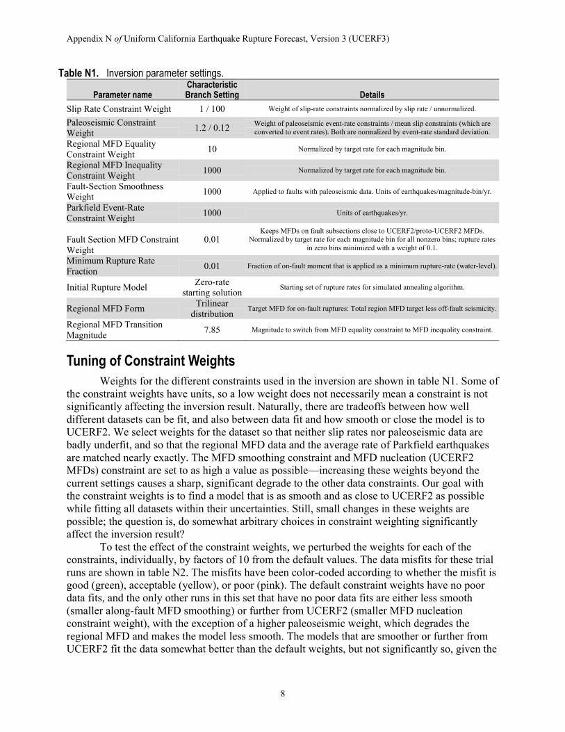
Table N1. Inversion parameter settings.

Parameter name Characteristic Branch Setting Details

Slip Rate Constraint Weight 1 / 100 Weight of slip-rate constraints normalized by slip rate / unnormalized.

Paleoseismic Constraint Weight 1.2 / 0.12 Weight of paleoseismic event-rate constraints / mean slip constraints (which are

converted to event rates). Both are normalized by event-rate standard deviation.

Regional MFD Equality Constraint Weight 10 Normalized by target rate for each magnitude bin.

Regional MFD Inequality Constraint Weight 1000 Normalized by target rate for each magnitude bin.

Fault-Section Smoothness Weight 1000 Applied to faults with paleoseismic data. Units of earthquakes/magnitude-bin/yr.

Parkfield Event-Rate Constraint Weight 1000 Units of earthquakes/yr.

Fault Section MFD Constraint Weight

0.01 Keeps MFDs on fault subsections close to UCERF2/proto-UCERF2 MFDs.

Normalized by target rate for each magnitude bin for all nonzero bins; rupture rates in zero bins minimized with a weight of 0.1.

Minimum Rupture Rate Fraction 0.01 Fraction of on-fault moment that is applied as a minimum rupture-rate (water-level).

Initial Rupture Model Zero-rate starting solution Starting set of rupture rates for simulated annealing algorithm.

Regional MFD Form Trilinear distribution Target MFD for on-fault ruptures: Total region MFD target less off-fault seismicity.

Regional MFD Transition Magnitude 7.85 Magnitude to switch from MFD equality constraint to MFD inequality constraint.

Tuning of Constraint Weights Weights for the different constraints used in the inversion are shown in table N1. Some of

the constraint weights have units, so a low weight does not necessarily mean a constraint is not significantly affecting the inversion result. Naturally, there are tradeoffs between how well different datasets can be fit, and also between data fit and how smooth or close the model is to UCERF2. We select weights for the dataset so that neither slip rates nor paleoseismic data are badly underfit, and so that the regional MFD data and the average rate of Parkfield earthquakes are matched nearly exactly. The MFD smoothing constraint and MFD nucleation (UCERF2 MFDs) constraint are set to as high a value as possible—increasing these weights beyond the current settings causes a sharp, significant degrade to the other data constraints. Our goal with the constraint weights is to find a model that is as smooth and as close to UCERF2 as possible while fitting all datasets within their uncertainties. Still, small changes in these weights are possible; the question is, do somewhat arbitrary choices in constraint weighting significantly affect the inversion result?

To test the effect of the constraint weights, we perturbed the weights for each of the constraints, individually, by factors of 10 from the default values. The data misfits for these trial runs are shown in table N2. The misfits have been color-coded according to whether the misfit is good (green), acceptable (yellow), or poor (pink). The default constraint weights have no poor data fits, and the only other runs in this set that have no poor data fits are either less smooth (smaller along-fault MFD smoothing) or further from UCERF2 (smaller MFD nucleation constraint weight), with the exception of a higher paleoseismic weight, which degrades the regional MFD and makes the model less smooth. The models that are smoother or further from UCERF2 fit the data somewhat better than the default weights, but not significantly so, given the


9

Table N2. Data misfits for alternative equation set weights. Misfits are coded as good acceptable poor

[The reference branch is in bold in the center row; wt, weight; avg., average; MFD, magnitude-frequency distribution]

Equation set weights Data misfits

Slip rate wt (normalized/

unnormalized)

Paleo wt (event rate / avg. slip)

Regional MFD wt

Fault section MFD wt

Fault section smoothness

Wt

Regional MFD misfit

Paleo event rate

misfit

Paleo slip misfit

Slip rate misfit

0.1 / 10 1.2 / 0.12 10 0.01 1000 0.00013 1.64 92.17 0.06946

1 / 100 0.12 / 0.012 10 0.01 1000 0.01645 134.40 204.57 0.00652

1 / 100 1.2 / 0.12 1 0.01 1000 10.50161 8.46 91.58 0.00535 1 / 100 1.2 / 0.12 10 0.001 1000 0.04151 13.57 92.88 0.00839 1 / 100 1.2 / 0.12 10 0.01 100 0.04051 9.53 110.73 0.00845 1 / 100 1.2 / 0.12 10 0.01 1000 0.03963 18.26 117.12 0.00867 1 / 100 1.2 / 0.12 10 0.01 10000 0.05043 35.66 158.79 0.01004 1 / 100 1.2 / 0.12 10 0.1 1000 0.04229 21.88 173.78 0.01580 1 / 100 1.2 / 0.12 100 0.01 1000 0.00004 47.18 183.52 0.02925 1 / 100 12 / 1.2 10 0.01 1000 0.16739 1.11 41.18 0.01869 10 / 1000 1.2 / 0.12 10 0.01 1000 6.97045 87.38 110.87 0.00351

Figure N3. Graphs showing hazard implications for the UCERF3 reference branch with alternative equation set weights (red lines show mean and min/max) compared to different branches of the UCERF2 logic tree (blue line and light blue area show mean and range spanned by min/max over 720 logic-tree branches with Fault Model 3.1).

loss of regularization. We can also see that fits to the slip rates and paleoseismic data strongly trade off against each other; this is in part due to the regional MFD constraint, which limits the extent that the inversion can alter the size distribution along faults to fit both slip rate and paleoseismic data.

Most importantly, figure N3 shows that changes in the constraint weights matter little for hazard, even when changes are large enough to cause some data to be poorly fit. The range of


10

hazard implications for the test inversion runs with different constraint weights is far less than the range of hazard spanned by different branches of the UCERF3 logic tree. These results imply that it is acceptable to use one set of weights for all inversion runs because changes in these weights (which would have to be smaller than the factors of 10 investigated here in order to not lead to poor data fits or a significantly less regularized model) are not important for hazard.

The regional MFD constraint has a high weight in the inversion and is fit very well by UCERF3 models; this is to prevent the MFD over-prediction (the “bulge”) that occurred in UCERF2 (Working Group on California Earthquake Probabilities, 2007). This constraint is surprisingly powerful; when removed, the inversion has enormous freedom to fit the slip rates, for example, nearly perfectly. It is informative to relax this constraint to see how it changes the model. MFD fits for the reference branch with the regional MFD constraint weight relaxed by a factor of 10 are shown in figure N4. We can see that the inversion prefers more moment—interestingly, at all magnitudes. This model, corresponding to the “Relax MFD” branch, which is currently given zero weight in the UCERF3 logic tree, is very well captured by the logic tree branches that increase the MFD target uniformly.

Figure N4. Graph showing magnitude-frequency distributions (MFDs) for a model where the MFD constraint weight is relaxed, which allows the model to fit other data better at the expense of the fit to the MFD target. This demonstrates that the other constraints could be better fit if more moment were put on faults relative to the amount allowed by target MFD.

Parkfield and Creeping Section Moment-Rate Reduction Tuning Creep is accounted for in the model in two ways: as a reduction of seismogenic fault area

and as a reduction in seismic slip rate. Area reduction due to creep, in UCERF parlance, is


11

termed an aseismicity factor; slip rate is reduced by applying a coupling coefficient less than 1 (for more details, see the main text of this report).

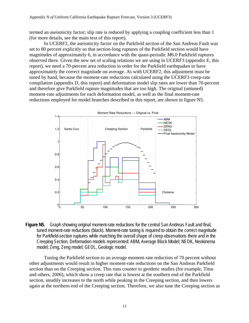
In UCERF2, the aseismicity factor on the Parkfield section of the San Andreas Fault was set to 80 percent explicitly so that section-long ruptures of the Parkfield section would have magnitudes of approximately 6, in accordance with the quasi-periodic M6.0 Parkfield ruptures observed there. Given the new set of scaling relations we are using in UCERF3 (appendix E, this report), we need a 70-percent area reduction in order for the Parkfield earthquakes to have approximately the correct magnitude on average. As with UCERF2, this adjustment must be tuned by hand, because the moment-rate reductions calculated using the UCERF3 creep-rate compilation (appendix D, this report) and deformation model slip rates are lower than 70-percent and therefore give Parkfield rupture magnitudes that are too high. The original (untuned) moment-rate adjustments for each deformation model, as well as the final moment-rate reductions employed for model branches described in this report, are shown in figure N5.

Figure N5. Graph showing original moment-rate reductions for the central San Andreas Fault and final, tuned moment-rate reductions (black). Moment-rate tuning is required to obtain the correct magnitude for Parkfield-section ruptures while matching the overall shape of creep observations there and in the Creeping Section. Deformation models represented: ABM, Average Block Model; NEOK, Neokinema model; Zeng, Zeng model; GEOL, Geologic model.

Tuning the Parkfield section to an average moment-rate reduction of 70 percent without other adjustments would result in higher moment-rate reductions on the San Andreas Parkfield section than on the Creeping section. This runs counter to geodetic studies (for example, Titus and others, 2006), which show a creep rate that is lowest at the southern end of the Parkfield section, steadily increases to the north while peaking in the Creeping section, and then lowers again at the northern end of the Creeping section. Therefore, we also tune the Creeping section as


12

well. Our final model is designed so that (a) section-long ruptures in the Parkfield section have a magnitude of approximately 6, (b) moment reductions increase smoothly from the southern end of the Parkfield section to the Creeping section, with a smooth “rainbow” shape in the Creeping section as suggested by geodetic models, (c) peak moment-rate reductions in the Creeping section exceed peak moment-rate reductions in the Parkfield section, (d) all moment-rate reductions in the Parkfield section are reductions to area, rather than slip rate (moment-rate reductions to slip rate do not affect magnitude), and (e) some moment-rate reduction in the Creeping section is applied to slip rate, which limits the rate of throughgoing ruptures allowed in the inversion.

Our tuned moment-rate reduction model, shown in black in figure N5, is far smoother than the original moment-rate reductions, since these are applied for deformation model mini-sections (appendix C, this report), which are larger than the approximately 7-km-long inversion subsections. Parkfield-section-long rupture magnitudes do have dependence on the scaling model used for the magnitude-area relation; our moment rate reductions give M6.15, M6.03, and M6.04 for the Ellsworth-B (Working Group on California Earthquake Probabilities, 2003), Hanks and Bakun (2008), and Shaw (2009) scaling relationships, respectively.

With our adjustments, the peak moment-rate reduction in the Creeping section is 98 percent. The first 90 percent of the moment-rate reduction is applied as an area reduction, and the remaining reduces the slip rate (that is, it lowers the coupling coefficient, as described in the main text of this report). This gives a maximum slip-rate reduction of 80 percent in the center of the Creeping section, which limits the rate of ruptures that rupture from one side of this section to the other. These reductions are used in the UCERF3 results described below and result in average repeat times for “wall-to-wall” San Andreas ruptures that extend from the (center of) SAF-Offshore to the SAF-Coachella section of 150,000 years. Ruptures for this model that extend from the SAF-North Coast to SAF-Mojave South section occur approximately every 2,500 years, and ruptures that extend (just barely) through the Creeping section, from SAF-Parkfield to SAF-Santa Cruz, occur every 900 years.

Defining the Set of Possible Fault-Based Ruptures A final a priori step that must be done before running the inversion is defining the set of

possible ruptures. The faults are first discretized into subsections, as described in UCERF3 (main text, this report). These subsections are specified for numerical tractability and do not represent geologic segments. Subsections are linked together to form ruptures, the rates of which are solved for by the inversion. It is worth noting that here a “rupture” is defined as an ordered list of fault subsections it includes; no hypocenter is specified.

Viable ruptures are generated from the digitized fault subsections via the plausibility filter rules described in detail by appendix T (this report). The plausibility filter defines a total of 253,706 ruptures for Fault Model 3.1 and 305,709 ruptures for Fault Model 3.2. By comparison, our UCERF2 mapping has (for a smaller set of faults) 7,029 on-fault ruptures.

One important remaining question is to what extent ruptures allowed by the plausibility rules may require further penalty. Because the inversion fits fault slip rates and the regional magnitude-frequency distribution, the frequency of multi-fault ruptures is already constrained. However, one could impose an additional “improbability” constraint to further penalize any ruptures that are deemed possible but improbable; these constraints are numerically equivalent to an a priori rupture-rate constraint with a rupture rate of zero. These constraints could be weighted individually, so some rupture rates could be penalized more harshly (that is, contribute more to


13

the misfit if they are nonzero) than others. This improbability constraint is not implemented for the UCERF3 rupture set since we do not have a viable model (that is, a model ready for implementation and agreed to be useful by WGCEP members) for such a constraint. Below we present evidence that this constraint is not needed, given empirical data and existing rupture-rate penalties.

It is not even clear what constitutes a “multi-fault” rupture in the case of a complex, possibly fractal, connected fault network. One way to quantify the rate of multi-fault ruptures is to simply define “multi-fault” in the context of the names assigned to faults in the UCERF3 database. For this definition of multi-fault, we count all sections of a fault such as the San Andreas Fault as one “named fault” even though the individual sections have different names (for example, Carrizo, Mojave North, and so forth). Using the inverted rupture rates for the UCERF3 reference branch model, 40 percent of M≥7 ruptures and only 16 percent of paleoseismically visible ruptures are on multiple faults. We can compare this number to the ruptures in the Wesnousky database of surface ruptures (Wesnousky, 2008); of these, 50 percent, or 14 out of 28, are on multiple faults. So by this albeit simple metric, the solutions given by the inversion algorithm are not producing more multi-fault ruptures than are seen in nature.

Figure N6. Graph showing rates of ruptures with different numbers of fault-to-fault jumps for the UCERF3 rupture set (green dashed line) and UCERF3 model (solid green line). Here a “jump” is defined as a pair of adjacent subsections in the rupture that are greater than 1 km apart, in 3D, as defined by our fault model. The empirical data are shown in blue. By this metric, the inversion model does not have as many multi-fault ruptures as the empirical data.

Another multi-fault metric from our model that we can compare to empirical data from the Wesnousky database is the rate of ruptures that have no jumps between faults versus 1, 2, or 3 jumps greater than 1 km. This comparison is shown in figure N6. This figure shows that the inversion constraints greatly reduce the rate of multi-fault ruptures in the solution relative to their frequency in the rupture set. Also, by this metric, the inversion is, again, underpredicting the rate


14

of multi-fault ruptures relative to the empirical data. We would even further underpredict the rates of ruptures with jumps if an improbability constraint were added to the inversion.

It is important to note that many of the truly multi-fault ruptures seen in nature may in fact not be part of our model at all because they could link up known, mapped faults with unknown faults (or faults that are known but not sufficiently studied as to be included in our fault model). Our model completely separates “on-fault” ruptures from background earthquakes; there are no ruptures that are partly “on-fault” and partly “off-fault”.

Without the improbability constraint, the inversion is not likely to give a lower rate to a rupture that is only moderately kinematically compatible (but allowed by our filters) relative to a more kinematically favored rupture, unless kinematically less favored jumps are also disfavored by slip-rate changes. However, the most egregious fault-to-fault jumps are already excluded by the Coulomb criteria described in appendix T (this report). It appears that the slip-rate constraints and rupture filtering leave only a modest amount of multi-fault ruptures in the inversion solution; further penalties to multi-fault ruptures will result in larger deviations from the empirical data.

The Simulated Annealing Algorithm We use a simulated annealing (SA) algorithm to solve the nonnegative least-squares

problem 𝐴𝑥 = 𝑑 with the additional constraint 𝐴𝑖𝑛𝑒𝑞𝑥 ≤ 𝑑𝑖𝑛𝑒𝑞 (this last constraint is due to the regional MFD inequality constraint). The SA algorithm simulates the slow cooling of a physical material to form a crystal. In the same way that annealing a metal reduces defects and allows the material to reach a lower thermodynamic energy, the simulated annealing algorithm attempts to minimize energy (in simulated annealing parlance this is the summed squared misfit between the data and synthetics) by slowly decreasing the probability of jumps to worse solutions. The algorithm we employ has the following steps: 1) Set x equal to initial solution 𝑥0. We have tested different initial solutions; the final UCERF3

model uses an initial solution of all zeros. 2) Lower the parameter 𝑇, known as the “temperature,” from 1 to 0 over a specified number of

iterations. We lower the temperature linearly, although different approaches to annealing specify different cooling functions, as we discuss in the section “Testing of Inversion Methodology.” Over each simulated annealing iteration: a) One element of 𝑥 (one rupture rate) is chosen at random. This element is then perturbed

randomly. It is here that the nonnegativity constraint is applied—the perturbation function is a function of the rupture rate and will not perturb the rate to a negative value. Unlike some simulated annealing algorithms, our algorithm does not use smaller perturbations as the temperature is lowered (this was tested but did not result in faster convergence times).

b) The misfit for the perturbed vector 𝑥, 𝑥𝑛𝑒𝑤, is calculated, and from this the “energy” of that solution: 𝐸𝑛𝑒𝑤 = (𝐴𝑥𝑛𝑒𝑤 − 𝑑)2 + 𝐸𝑖𝑛𝑒𝑞 , where 𝐸𝑖𝑛𝑒𝑞 is additional energy from the MFD inequality constraint: 𝐸𝑖𝑛𝑒𝑞 = (min (𝐴𝑖𝑛𝑒𝑞 𝑥𝑛𝑒𝑤 − 𝑑𝑖𝑛𝑒𝑞, 0))2. The weight on the inequality constraint is set quite high so that a solution that violates it faces a significant penalty; thus, in practice, this is a strict inequality constraint.

c) The transition probability 𝑃 is calculated based on the change in energy (between the previous state and the perturbed state) and the current temperature 𝑇. If the new model is better, 𝑃 = 1. Therefore, a new model is always kept if it is better. If the new model is


15

worse, it is sometimes kept, and this is more likely early in the annealing process when the temperature is high. If 𝐸 < 𝐸𝑛𝑒𝑤, 𝑃 = 𝑒(𝐸−𝐸𝑛𝑒𝑤)/𝑇.

3) Once the annealing schedule is completed, the best solution x found during the search (the solution with the lowest energy) is returned. (Note that this is a common departure from “pure” simulated annealing, which returns the last state found. In some cases the final state will not be the best solution found, because occasionally solutions are discarded for worse solutions).

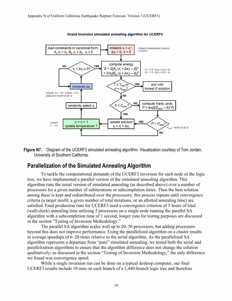
The UCERF3 SA algorithm is shown graphically in the flowchart in figure N7. Simulated annealing works similarly to other nonlinear algorithms such as the genetic

algorithm (Holland, 1975). One advantage of simulated annealing is that there is a strong theoretical backing: besides the analogy to annealing a physical material, the simulated annealing algorithm will find the global minimum misfit given infinite cooling time, provided that the annealing schedule lowers the temperature sufficiently slowly (Granville and others, 1994).

There are several advantages of this algorithm over other approaches such as the nonnegative least-squares algorithm. First, the simulated annealing algorithm scales well as the problem size increases. (In fact, it would not be computationally feasible for us to use the nonnegative least-squares algorithm to solve a problem as large as the UCERF3 grand inversion.) Simulated annealing is designed to efficiently search a large parameter space without getting stuck in local minima. Next, quite importantly, for an underdetermined problem the simulated annealing algorithm gives multiple solutions (at varying levels of misfit depending on the annealing schedule). Thus both the resolution error (the range of models that satisfy one realization of the data) and the data error (the impact of parameter uncertainty on the model) can be sampled. Finally, simulated annealing allows us to include other nonlinear constraints in the inversion apart from nonnegativity; in our case we incorporate the MFD inequality constraint, which is a nonlinear constraint that cannot be easily incorporated into the perturbation function.


16

Figure N7. Diagram of the UCERF3 simulated annealing algorithm. Visualization courtesy of Tom Jordan, University of Southern California.

Parallelization of the Simulated Annealing Algorithm To tackle the computational demands of the UCERF3 inversion for each node of the logic

tree, we have implemented a parallel version of the simulated annealing algorithm. This algorithm runs the serial version of simulated annealing (as described above) over a number of processors for a given number of subiterations or subcompletion times. Then the best solution among these is kept and redistributed over the processors; this process repeats until convergence criteria (a target misfit, a given number of total iterations, or an allotted annealing time) are satisfied. Final production runs for UCERF3 used a convergence criterion of 5 hours of total (wall-clock) annealing time utilizing 5 processors on a single node running the parallel SA algorithm with a subcompletion time of 1 second; longer runs for testing purposes are discussed in the section “Testing of Inversion Methodology.”

The parallel SA algorithm scales well up to 20–50 processors, but adding processors beyond this does not improve performance. Using the parallelized algorithm on a cluster results in average speedups of 6–20 times relative to the serial algorithm. As the parallelized SA algorithm represents a departure from “pure” simulated annealing, we tested both the serial and parallelization algorithms to ensure that the algorithm difference does not change the solution qualitatively; as discussed in the section “Testing of Inversion Methodology,” the only difference we found was convergence speed.

While a single inversion run can be done on a typical desktop computer, our final UCERF3 results include 10 runs on each branch of a 1,440-branch logic tree and therefore


17

required 3,000 node-days of computation time. We used the Stampede cluster at the University of Texas and the HPCC cluster at the University of Southern California to run all the inversions required for the UCERF3 branches in under a day.

Testing of Inversion Methodology Convergence Properties

The simulated annealing algorithm used in UCERF3 is stochastic; because of random perturbations of the model parameters during the annealing process, the final model will be different each time it is run, even if the starting model and data do not change. This can be an advantage because it allows us to explore the range of models that fit the data on a single branch; however, finding a stable solution can present a challenge. We have extensively tested the convergence properties of the inversion and found that over individual runs, unsurprisingly, individual rupture rates are very poorly constrained and are highly variable. However, averaged parameters such as fault section MFDs are far more robust.

In a single run of the inversion, only about 10,000 ruptures (~ 4 percent) have rates above the water-level rates. This demonstrates that the data can be fit with a relatively small subset of ruptures. By averaging more runs, however, more of the ruptures have rates above the water level. For a single branch, averaging 10 runs increases the number of ruptures above the water level to approximately 38,000, and averaging 200 runs increases this number to approximately 115,000. Different runs of the same branch therefore match the data similarly well by using different sets of ruptures and are sampling the epistemic uncertainty of the problem in this way. Averaging across branches achieves smoother, less compact results; the average of 10 branches for all 720 logic-tree branches in Fault Model 3.1 produces 93 percent of ruptures above the water-level rates.

For many faults, stable parameters of the rate a given fault section participates in a rupture of a given magnitude can be determined from averaging only a few inversion runs; the median number of inversion runs needed to resolve the mean rate of M≥6.7 events on a fault within 10 percent is 9. A small number of slow-moving faults require on the order of 100 runs to obtain well-resolved magnitude distributions; as discussed elsewhere in this report (main text)—the worst case is the Richfield Fault (a 2-subsection-long fault near the Whittier Fault), which requires 1,294 runs. As the branch-averaged UCERF3 model (Mean UCERF3) uses results from 14,400 individual SA runs, all faults have magnitude-frequency distributions that are well resolved.

Hazard results, as shown in figure N8, are even more stable across inversion runs. Of the 2-percent-in-50-years and 1-percent-in-100-years annual frequencies of exceedance for peak ground acceleration (PGA), and spectral accelerations at 5 Hz, 1 Hz, and 4 seconds, the worst uncertainty we found over 10 runs of the UCERF3 reference branch was within 3 percent of the mean, as described in the main text of this report. Thus individual branches of the logic tree, each of which average more than 10 SA runs, are well resolved for all these hazard metrics. Branch-averaged results are extremely well resolved for hazard metrics; in fact, inversion nonuniqueness was found to be negligible for the 2-percent-in-50-years PGA, 1-percent-in-100-years PGA, and 2-percent-in-50-years hazard maps, as well as the 1-percent-in-100-years 3-second spectral acceleration hazard maps. In fact, a single SA run per branch would be adequate for these hazard metrics.


18

Figure N8. Graphs showing convergence test results for hazard curves from 200 runs of the UCERF3 reference branch. For Los Angeles (left) and San Francisco (middle), the range of hazard curves from multiple runs (light blue) is so small that it is not visible behind the mean hazard curve over all runs (dark blue curve). We also show a hazard curve for Diablo Canyon (right), because in this case differences between different inversion runs for the reference branch are visible at very low annual frequencies of exceedance; this is the largest variance among the 60 test locations.

Synthetic Test

To test the ability of the inversion method to recover a solution, we create a synthetic test based on the inversion synthetics from the UCERF3 reference branch. The data used include the slip rate, paleoseismic data, regional magnitude distribution, fault section MFD, and Parkfield event-rate synthetics. The magnitude-distribution smoothing constraint (used on fault sections with paleoseismic data) was applied as in a typical inversion, without using the reference branch synthetics. No errors were added to the input data. Misfits in the synthetic test demonstrate how well the inversion converges, and differences between different runs of the synthetic test give a sense of the null space of the problem. Slip-rate fits for multiple runs of this synthetic test are shown in figure N9.

Figure N9. Maps showing slip-rate fits from five synthetic test runs (using the zero starting solution).


19

The total squared misfit of the slip rates in the synthetic test is 18 times less than that for the UCERF3 reference branch. The largest systematic discrepancy on the major faults is an overprediction of the slip rate of approximately 10 percent on the Mojave South section of the Southern San Andreas Fault. In addition, the southern end of the Ozena Fault and the Swain Ravine Fault have slip rates that are more severely overpredicted and underpredicted, respectively. These systematics are not persistent features of UCERF3 inversion runs.

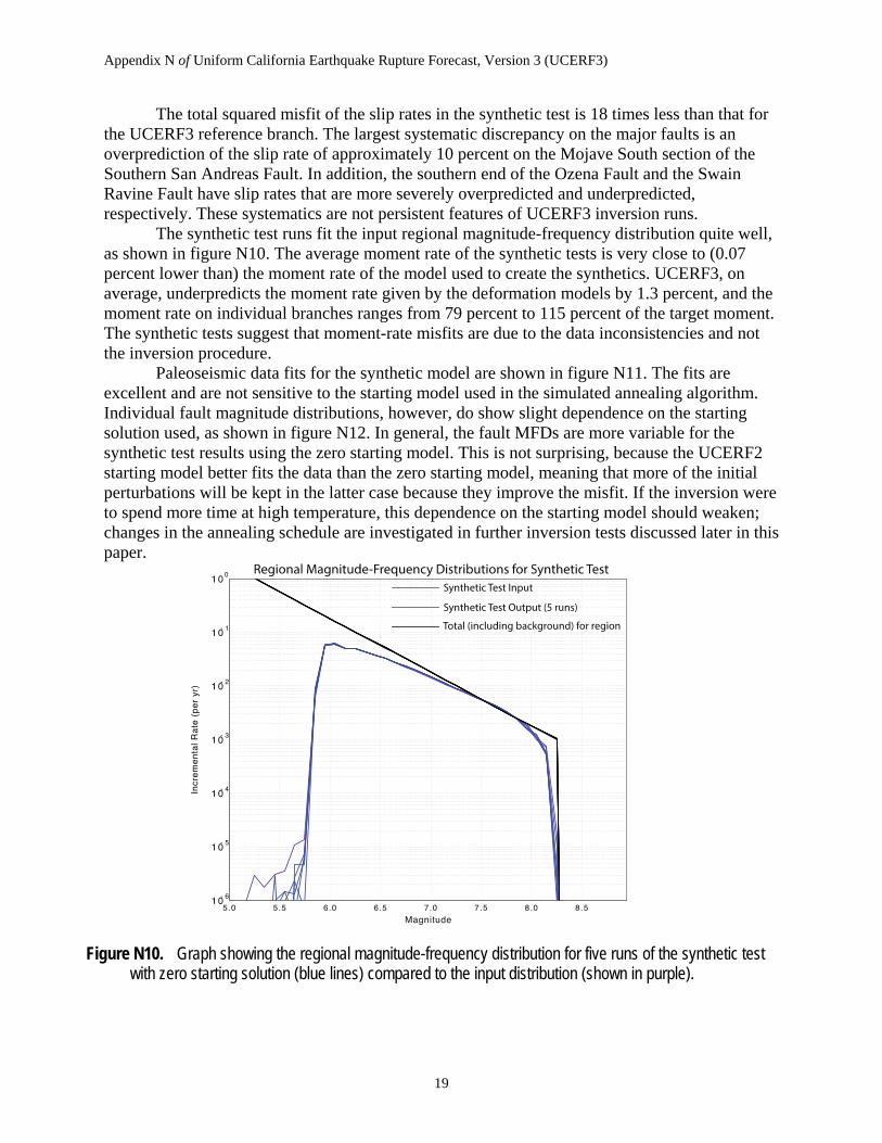
The synthetic test runs fit the input regional magnitude-frequency distribution quite well, as shown in figure N10. The average moment rate of the synthetic tests is very close to (0.07 percent lower than) the moment rate of the model used to create the synthetics. UCERF3, on average, underpredicts the moment rate given by the deformation models by 1.3 percent, and the moment rate on individual branches ranges from 79 percent to 115 percent of the target moment. The synthetic tests suggest that moment-rate misfits are due to the data inconsistencies and not the inversion procedure.

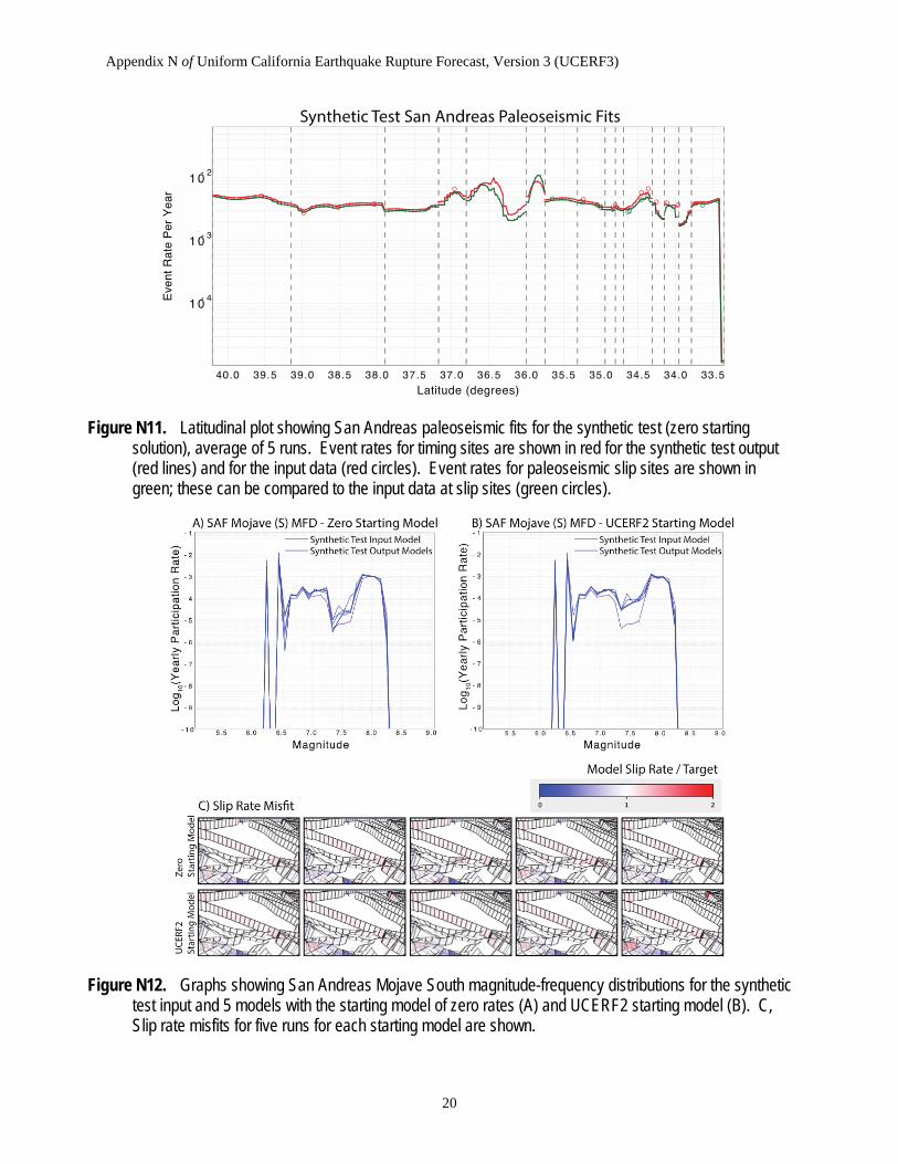
Paleoseismic data fits for the synthetic model are shown in figure N11. The fits are excellent and are not sensitive to the starting model used in the simulated annealing algorithm. Individual fault magnitude distributions, however, do show slight dependence on the starting solution used, as shown in figure N12. In general, the fault MFDs are more variable for the synthetic test results using the zero starting model. This is not surprising, because the UCERF2 starting model better fits the data than the zero starting model, meaning that more of the initial perturbations will be kept in the latter case because they improve the misfit. If the inversion were to spend more time at high temperature, this dependence on the starting model should weaken; changes in the annealing schedule are investigated in further inversion tests discussed later in this paper.

Figure N10. Graph showing the regional magnitude-frequency distribution for five runs of the synthetic test with zero starting solution (blue lines) compared to the input distribution (shown in purple).


20

Figure N11. Latitudinal plot showing San Andreas paleoseismic fits for the synthetic test (zero starting solution), average of 5 runs. Event rates for timing sites are shown in red for the synthetic test output (red lines) and for the input data (red circles). Event rates for paleoseismic slip sites are shown in green; these can be compared to the input data at slip sites (green circles).

Figure N12. Graphs showing San Andreas Mojave South magnitude-frequency distributions for the synthetic test input and 5 models with the starting model of zero rates (A) and UCERF2 starting model (B). C, Slip rate misfits for five runs for each starting model are shown.


21

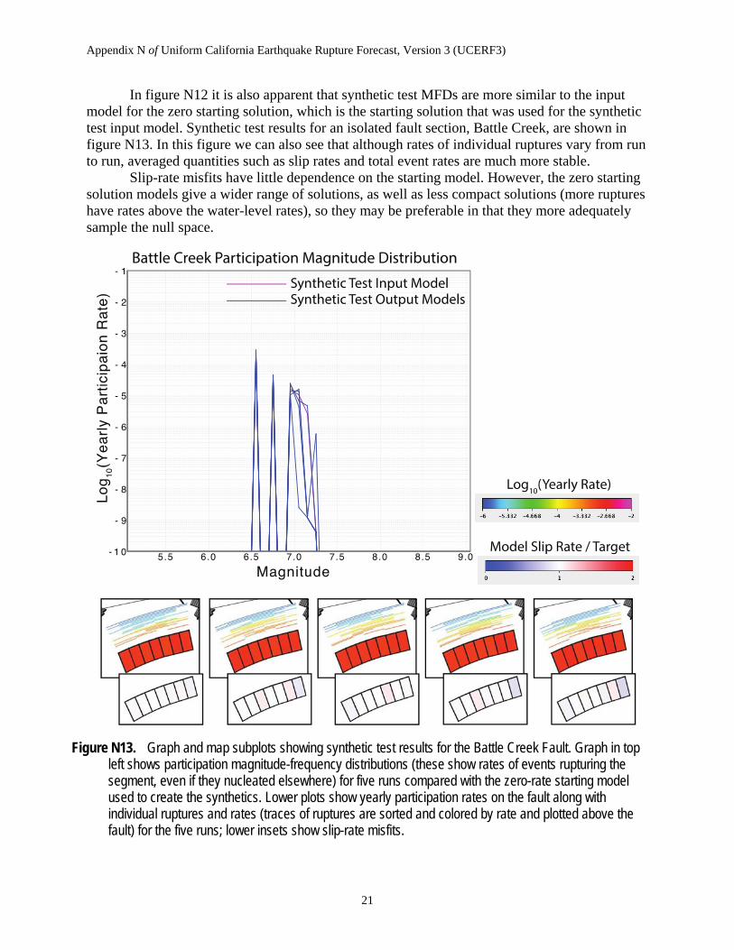
In figure N12 it is also apparent that synthetic test MFDs are more similar to the input model for the zero starting solution, which is the starting solution that was used for the synthetic test input model. Synthetic test results for an isolated fault section, Battle Creek, are shown in figure N13. In this figure we can also see that although rates of individual ruptures vary from run to run, averaged quantities such as slip rates and total event rates are much more stable.

Slip-rate misfits have little dependence on the starting model. However, the zero starting solution models give a wider range of solutions, as well as less compact solutions (more ruptures have rates above the water-level rates), so they may be preferable in that they more adequately sample the null space.

Figure N13. Graph and map subplots showing synthetic test results for the Battle Creek Fault. Graph in top left shows participation magnitude-frequency distributions (these show rates of events rupturing the segment, even if they nucleated elsewhere) for five runs compared with the zero-rate starting model used to create the synthetics. Lower plots show yearly participation rates on the fault along with individual ruptures and rates (traces of ruptures are sorted and colored by rate and plotted above the fault) for the five runs; lower insets show slip-rate misfits.


22

Alternative Simulated Annealing Algorithms We tested a variety of published perturbation functions and c

𝑇

ooling functions to ensure that the s

𝑖

imulated annealing (SA) algorithm we are using is optimized for our problem. The cooling functions, which give the simulated annealing temperature as a function of iteration number , include:

• Classical SA (Geman and Geman, 1984):

• Fast SA (Szu and Hartley, 1987): • Very Fast SA (Ingber, 1989): 𝑇 =

𝑇𝑒−

=𝑖+1

𝑇 = 1/ log (𝑖 + 1)

𝑅 → [0 1]

The perturbation functions we tested, in uni

1/ 𝑖

ts of 1/year, as a function of a random number , are as follows:

• Uniform, no temperature dependence: • Gaussian:

Δ Δ𝑥𝑥 = 0.001 𝑇−1/2

Δ=𝑥

0=.001

sgn 𝑇(𝑅

tan−

( 𝜋𝑅𝑅 𝑒

−1/2

𝜋𝑇

0.5) (0.001/

• Tangent:

Δ𝑥

= 0.001(𝑅 − 0.5)

• Power Law: • Exponential:

2)

The normalizaΔt𝑥 001 𝑇 10𝑅 ion f

= 0a.ctors for

each of the

𝑇

a

)

bove

(1 + 1𝑇)|2𝑅−1|−1

functions have been optimized within a factor of 10 to produce the fastest convergence. We tested each combination of cooling schedules and perturbation functions for both the serial and parallel SA algorithms. For UCERF3 runs we use the Fast SA cooling schedule with uniform (no temperature dependence) perturbations. This produces the best final energies (and therefore lowest misfits) for both the parallel and serial simulated annealing algorithms, within the noise—that is, neglecting the small differences in final energies typically seen over multiple runs of the same inversion.

Long Cooling Test The simulated annealing algorithm more adequately searches the solution space with

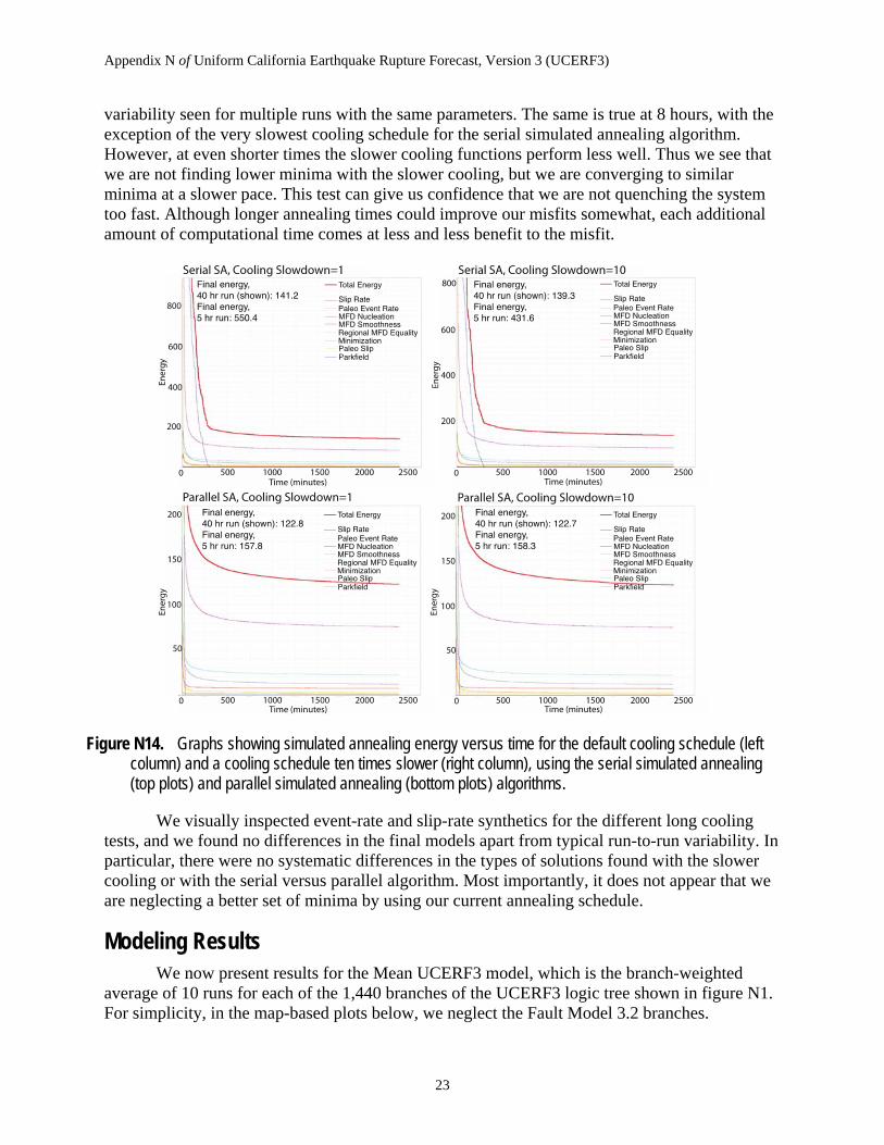
slower cooling schedules, although this also requires more computational time. Early in the simulated annealing, when temperature is high, jumps to worse solutions are more likely to be taken, and this is necessary in order to avoid getting stuck in local minima. Our default simulated annealing parameters have been chosen to achieve the lowest misfit for simulated annealing runs that take 4–8 hours; given the computational capacity we have at our disposal, this allows us to compute the entire UCERF3 model, with 10 runs of each branch, in under a day using supercomputers. To ensure that this annealing schedule is adequate we run a series of long cooling tests with the reference branch. Each is run for 40 hours in total, using both the serial and parallel algorithms, for the standard cooling schedule, and for schedules where the temperature is lowered 2, 5, and 10 times slower.

Figure N14 shows the simulated annealing energy (proportional to the squared misfit) versus time for the slow cooling tests. The parallel algorithm outperforms the serial algorithm, which is not surprising because it uses multiple processors and is searching more of the space (and represents more total computational time summed over all processors). However, the difference between the parallel and serial algorithm is less pronounced at longer times, which suggests that although the parallel algorithm converges faster, given enough time, the serial algorithm can catch up.

The speed of the cooling, at least within the range we tested, has negligible effect on the final energies at very long times. The differences at 40 hours between the test runs are within the


23

variability seen for multiple runs with the same parameters. The same is true at 8 hours, with the exception of the very slowest cooling schedule for the serial simulated annealing algorithm. However, at even shorter times the slower cooling functions perform less well. Thus we see that we are not finding lower minima with the slower cooling, but we are converging to similar minima at a slower pace. This test can give us confidence that we are not quenching the system too fast. Although longer annealing times could improve our misfits somewhat, each additional amount of computational time comes at less and less benefit to the misfit.

Figure N14. Graphs showing simulated annealing energy versus time for the default cooling schedule (left column) and a cooling schedule ten times slower (right column), using the serial simulated annealing (top plots) and parallel simulated annealing (bottom plots) algorithms.

We visually inspected event-rate and slip-rate synthetics for the different long cooling tests, and we found no differences in the final models apart from typical run-to-run variability. In particular, there were no systematic differences in the types of solutions found with the slower cooling or with the serial versus parallel algorithm. Most importantly, it does not appear that we are neglecting a better set of minima by using our current annealing schedule.

Modeling Results We now present results for the Mean UCERF3 model, which is the branch-weighted

average of 10 runs for each of the 1,440 branches of the UCERF3 logic tree shown in figure N1. For simplicity, in the map-based plots below, we neglect the Fault Model 3.2 branches.


24

In many of the figures below we compare the UCERF3 model to UCERF2, or rather, a mapping of UCERF2 into our rupture set. For this mapped UCERF2 model, we set the magnitudes of ruptures to their mean UCERF2 values (neglecting aleatory variable in magnitude) and average (with 50-percent weight each) a tapered along-strike slip distribution and a uniform slip distribution for each rupture (these are the same weights used for the along-strike slip distributions in UCERF3).

UCERF3 Fits to Data UCERF3 is constrained to match slip-rate targets, as defined by the deformation models,

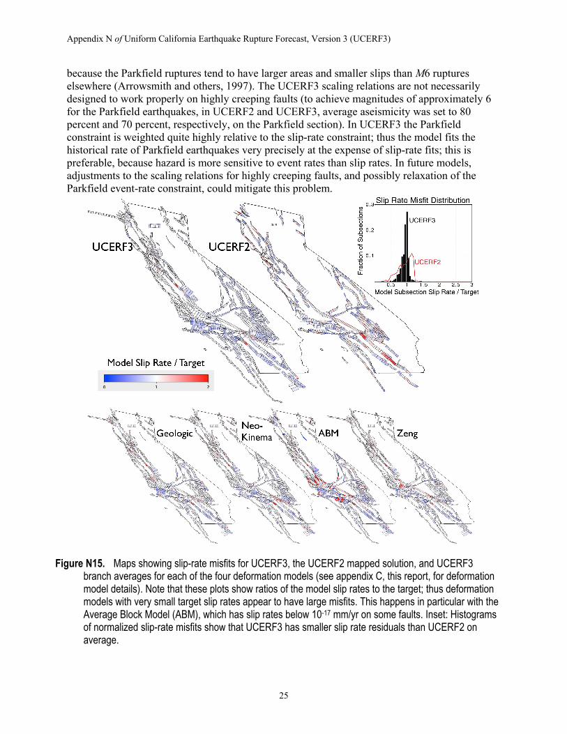
for each fault subsection. Figure N15 shows fits to the slip rates for UCERF2, Mean UCERF3, and branch-averaged solutions for each deformation model. The UCERF2 model tends to overpredict slip rates in the centers of fault sections and underpredict slip rates on the edges of fault sections. This is due to two effects: the 50-percent weight on the tapered along-strike slip distribution and the “floating” ruptures used in UCERF2—the set of ruptures for each magnitude bin allowed at different positions along a given fault section—which overlap more in the center. Slip-rate fits for the UCERF3 models are on the whole good, although individual branches have total moment rates ranging from 79 percent to 115 percent of the total on-fault target moment (this is the moment given by the deformation model, less creep and subseismogenic-rupture moment). Mean UCERF3 underpredicts the target moment rate by 1.3 percent.

The two biggest slip-rate overpredictions are on the Northern end of the Elsinore Fault and in the center of the Creeping section of the San Andreas Fault. The model overpredicts the target slip rate on the Elsinore Fault because of a high paleoseismic event rate on that fault. The outlier in the Creeping section occurs where the mean slip rate is reduced by 80 percent to 5 mm/year in order to account for creep. The inversion is unable to match this rapid along-strike slip-rate change; the solution only reduces the slip rate to approximately 10 mm/yr. All other UCERF3 slip-rate overpredictions are within 20 percent of the targets, and virtually all those greater than 10 percent can be explained by paleoseismic constraint inconsistencies. Furthermore, mean slip rates on all faults are within the error bounds given by the Geologic deformation model, even though these error bounds were not used in the inversion.

Slip-rate and paleoseismic data fits for the San Andreas Fault are shown in figure N16. The target slip rate is underpredicted on the Cholame section of the San Andreas, and this is systematic across different UCERF3 branches. If the regional MFD constraint is removed (thus allowing the inversion as many ruptures in a given magnitude range as needed to minimize misfits to other data), the slip rate on the Cholame section can be fit nearly perfectly.

However, given that the regional magnitude distribution allows for a limited budget for moderate-size earthquakes throughout the region, this slip-rate cannot be fit without increasing misfits to other constraints. Contributing to the problem is the tendency for many of the branches to overpredict the slip rate on the Parkfield section (and thus preventing more Cholame ruptures from continuing to the north). This is because much of the slip rate for the Parkfield section is taken up in Parkfield M~6 ruptures, which are constrained to have a mean recurrence interval of 25 years. The mean slip in the Parkfield ruptures ranges from 0.27–0.35 m for the Shaw (2009) scaling relation and the Hanks and Bakun (2008) scaling relation to 0.57–0.73 m for the Ellsworth-B (Working Group on California Earthquake Probabilities, 2003) scaling relation. Thus 10–29 mm/yr is taken up on the Parkfield section just in Parkfield M~6 ruptures, which leaves very little, if any, remaining moment for other ruptures on this fault section. The slips given by the scaling relations for the Parkfield ruptures are quite high, and perhaps too high,


25

because the Parkfield ruptures tend to have larger areas and smaller slips than M6 ruptures elsewhere (Arrowsmith and others, 1997). The UCERF3 scaling relations are not necessarily designed to work properly on highly creeping faults (to achieve magnitudes of approximately 6 for the Parkfield earthquakes, in UCERF2 and UCERF3, average aseismicity was set to 80 percent and 70 percent, respectively, on the Parkfield section). In UCERF3 the Parkfield constraint is weighted quite highly relative to the slip-rate constraint; thus the model fits the historical rate of Parkfield earthquakes very precisely at the expense of slip-rate fits; this is preferable, because hazard is more sensitive to event rates than slip rates. In future models, adjustments to the scaling relations for highly creeping faults, and possibly relaxation of the Parkfield event-rate constraint, could mitigate this problem.

Figure N15. Maps showing slip-rate misfits for UCERF3, the UCERF2 mapped solution, and UCERF3 branch averages for each of the four deformation models (see appendix C, this report, for deformation model details). Note that these plots show ratios of the model slip rates to the target; thus deformation models with very small target slip rates appear to have large misfits. This happens in particular with the Average Block Model (ABM), which has slip rates below 10-17 mm/yr on some faults. Inset: Histograms of normalized slip-rate misfits show that UCERF3 has smaller slip rate residuals than UCERF2 on average.


26

Figure N16. Latitudinal plots showing San Andreas slip-rate and paleoseismic data fits, respectively, for (A) and (B) UCERF2, and (C) and (D) UCERF3. Paleoseismic mean slip data have been converted to proxy event-rate data, shown by the green circles. The paleoseismic data in both subplots shown is from the UCERF3 model; UCERF2 mean paleoseismic event-rate data and error bounds were quite different in some locations. UCERF2 event rates plotted with UCERF2 data are shown in the main text of this report.


27

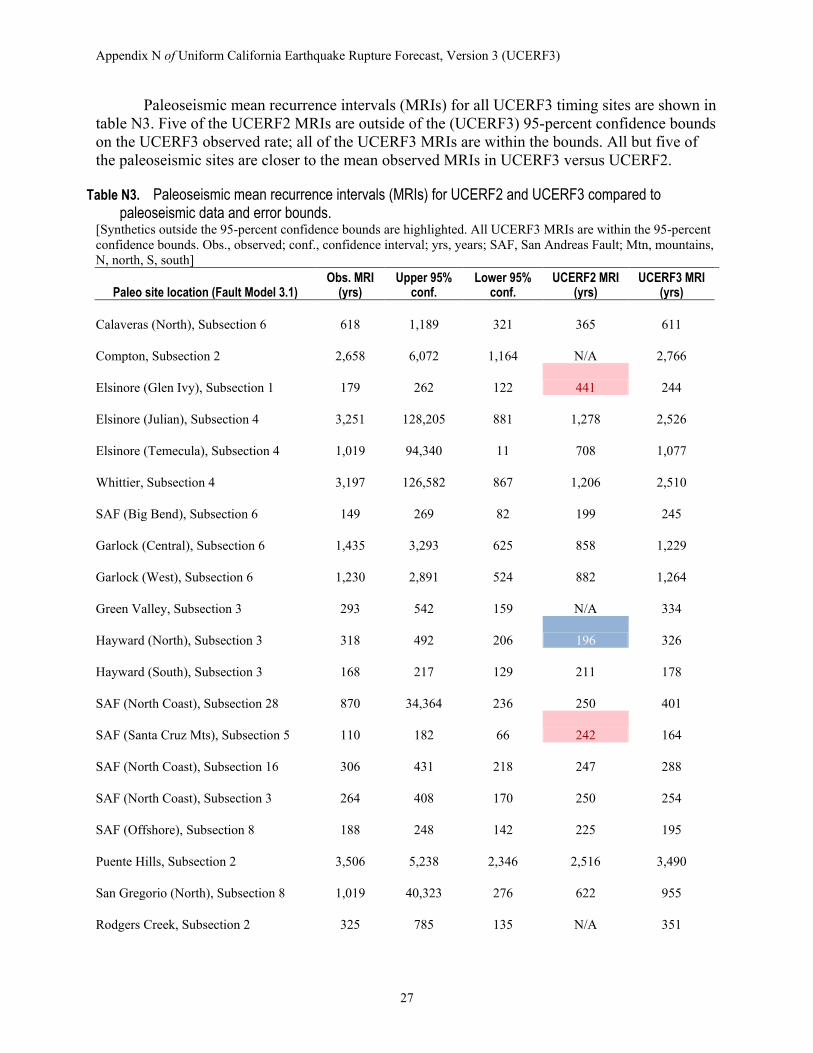
Paleoseismic mean recurrence intervals (MRIs) for all UCERF3 timing sites are shown in table N3. Five of the UCERF2 MRIs are outside of the (UCERF3) 95-percent confidence bounds on the UCERF3 observed rate; all of the UCERF3 MRIs are within the bounds. All but five of the paleoseismic sites are closer to the mean observed MRIs in UCERF3 versus UCERF2.

Table N3. Paleoseismic mean recurrence intervals (MRIs) for UCERF2 and UCERF3 compared to paleoseismic data and error bounds.

[Synthetics outside the 95-percent confidence bounds are highlighted. All UCERF3 MRIs are within the 95-percent confidence bounds. Obs., observed; conf., confidence interval; yrs, years; SAF, San Andreas Fault; Mtn, mountains, N, north, S, south]

Paleo site location (Fault Model 3.1) Obs. MRI

(yrs) Upper 95%

conf. Lower 95%

conf. UCERF2 MRI

(yrs) UCERF3 MRI

(yrs) Calaveras (North), Subsection 6 618 1,189 321 365 611

Compton, Subsection 2 2,658 6,072 1,164 N/A 2,766

Elsinore (Glen Ivy), Subsection 1 179 262 122 441 244

Elsinore (Julian), Subsection 4 3,251 128,205 881 1,278 2,526

Elsinore (Temecula), Subsection 4 1,019 94,340 11 708 1,077

Whittier, Subsection 4 3,197 126,582 867 1,206 2,510

SAF (Big Bend), Subsection 6 149 269 82 199 245

Garlock (Central), Subsection 6 1,435 3,293 625 858 1,229

Garlock (West), Subsection 6 1,230 2,891 524 882 1,264

Green Valley, Subsection 3 293 542 159 N/A 334

Hayward (North), Subsection 3 318 492 206 196 326

Hayward (South), Subsection 3 168 217 129 211 178

SAF (North Coast), Subsection 28 870 34,364 236 250 401

SAF (Santa Cruz Mts), Subsection 5 110 182 66 242 164

SAF (North Coast), Subsection 16 306 431 218 247 288

SAF (North Coast), Subsection 3 264 408 170 250 254

SAF (Offshore), Subsection 8 188 248 142 225 195

Puente Hills, Subsection 2 3,506 5,238 2,346 2,516 3,490

San Gregorio (North), Subsection 8 1,019 40,323 276 622 955

Rodgers Creek, Subsection 2 325 785 135 N/A 351


28

Paleo site location (Fault Model 3.1) Obs. MRI

(yrs) Upper 95%

conf. Lower 95%

conf. UCERF2 MRI

(yrs) UCERF3 MRI

(yrs)

San Jacinto (Anza), Subsection 3 312 549 177 256 363

San Jacinto (Superstition Mtn), Sub. 0 508 1687 153 401 509

SAF (Carrizo), Subsection 1 115 205 64 187 193

SAF (San Bernardino S), Subsection 6 205 354 119 312 289

SAF (Coachella), Subsection 1 178 321 99 162 259

SAF (Coachella), Subsection 1 277 449 171 162 259

SAF (Mojave S), Subsection 9 149 225 99 158 180

SAF (San Bernardino N), Subsection 2 173 284 106 190 249

SAF (San Bernardino S), Subsection 1 205 345 122 244 264 SAF (San Gorgonio Pass-Garnet HIll), Sub. 0 261 409 167 394 306

SAF (Mojave S), Subsection 13 106 148 76 174 138 One readily apparent systematic in the paleoseismic misfits is that paleoseismic

synthetics on the Southern San Andreas Fault are lower than the mean observed rates (recurrence intervals in the model are, on average, longer than observed). This is also the case with the UCERF2 model, although the UCERF2 paleoseismic data (see fig. 20 in the main text) had higher means and larger error bars on this fault. The Southern San Andreas Fault paleoseismic data could be better fit by increasing the weight on the paleoseismic data, but this would degrade the slip-rate fit and lead to (further) overfitting of the paleoseismic data in other areas. In fact, the reduced chi-squared value for the UCERF3 paleoseismic event-rate fits is 0.72. That this is less than 1 means that given the uncertainties, on the whole UCERF3 overfits the paleoseismic data. Although event rates on the Southern San Andreas Fault are systematically lower than the observed rates, it should be noted that these sites do not represent independent data. These sites are all seeing overlapping time periods on the San Andreas, which could have recent activity that is, together at all sites, above or below the long-term average. In addition, many events are seen in multiple, neighboring trenches, so the event rates measured at nearby different paleoseismic sites are not independent. Given the correlated data, the spatial systematics in the paleoseismic misfits are expected.

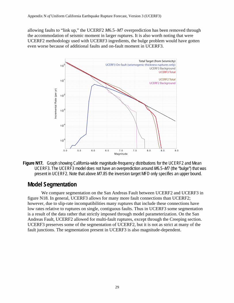
On-fault, off-fault, and total magnitude distributions for UCERF2 and UCERF3 are shown in figure N17. All branches of UCERF3 fit the target MFD quite well. At high magnitudes the regional magnitude-frequency distribution tapers away from the b=1 extrapolation (which does not contribute to the regional MFD misfit because the MFD constraint becomes an inequality constraint above M7.85). The background MFD is similar to, but smoother than, the background MFD in UCERF2. Most importantly, the inversion methodology eliminates the “bulge” problem in UCERF2—the overprediction of earthquakes around M6.5–M7. Through testing changes to the rupture set, we determined that fitting the MFD constraint and thus eliminating this “bulge” required multi-fault ruptures not included in UCERF2. By


29

allowing faults to “link up,” the UCERF2 M6.5–M7 overprediction has been removed through the accommodation of seismic moment in larger ruptures. It is also worth noting that were UCERF2 methodology used with UCERF3 ingredients, the bulge problem would have gotten even worse because of additional faults and on-fault moment in UCERF3.

Figure N17. Graph showing California-wide magnitude-frequency distributions for the UCERF2 and Mean UCERF3. The UCERF3 model does not have an overprediction around M6.5–M7 (the “bulge”) that was present in UCERF2. Note that above M7.85 the inversion target MFD only specifies an upper bound.

Model Segmentation We compare segmentation on the San Andreas Fault between UCERF2 and UCERF3 in

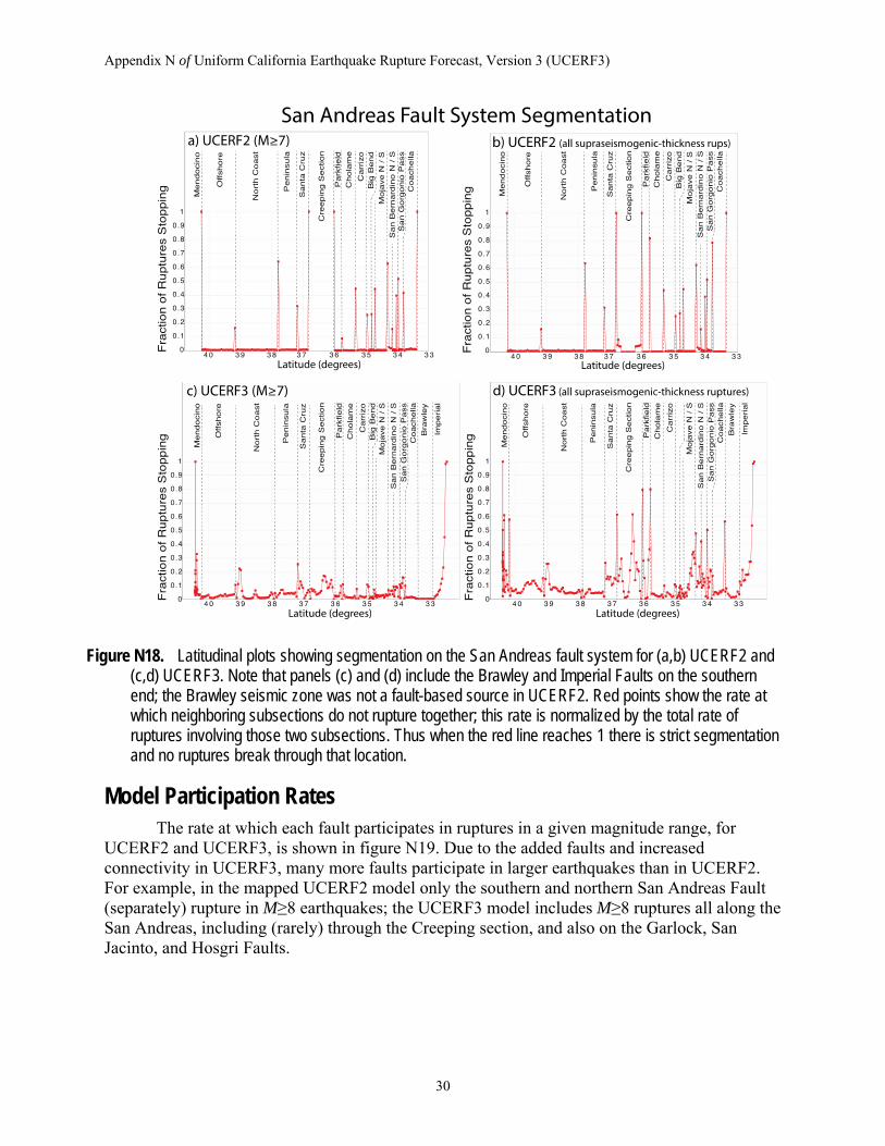
figure N18. In general, UCERF3 allows for many more fault connections than UCERF2; however, due to slip-rate incompatibilities many ruptures that include these connections have low rates relative to ruptures on single, contiguous faults. Thus in UCERF3 some segmentation is a result of the data rather that strictly imposed through model parameterization. On the San Andreas Fault, UCERF2 allowed for multi-fault ruptures, except through the Creeping section. UCERF3 preserves some of the segmentation of UCERF2, but it is not as strict at many of the fault junctions. The segmentation present in UCERF3 is also magnitude-dependent.


30

Figure N18. Latitudinal plots showing segmentation on the San Andreas fault system for (a,b) UCERF2 and (c,d) UCERF3. Note that panels (c) and (d) include the Brawley and Imperial Faults on the southern end; the Brawley seismic zone was not a fault-based source in UCERF2. Red points show the rate at which neighboring subsections do not rupture together; this rate is normalized by the total rate of ruptures involving those two subsections. Thus when the red line reaches 1 there is strict segmentation and no ruptures break through that location.

Model Participation Rates The rate at which each fault participates in ruptures in a given magnitude range, for

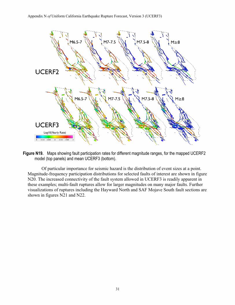
UCERF2 and UCERF3, is shown in figure N19. Due to the added faults and increased connectivity in UCERF3, many more faults participate in larger earthquakes than in UCERF2. For example, in the mapped UCERF2 model only the southern and northern San Andreas Fault (separately) rupture in M≥8 earthquakes; the UCERF3 model includes M≥8 ruptures all along the San Andreas, including (rarely) through the Creeping section, and also on the Garlock, San Jacinto, and Hosgri Faults.


31

Figure N19. Maps showing fault participation rates for different magnitude ranges, for the mapped UCERF2 model (top panels) and mean UCERF3 (bottom).

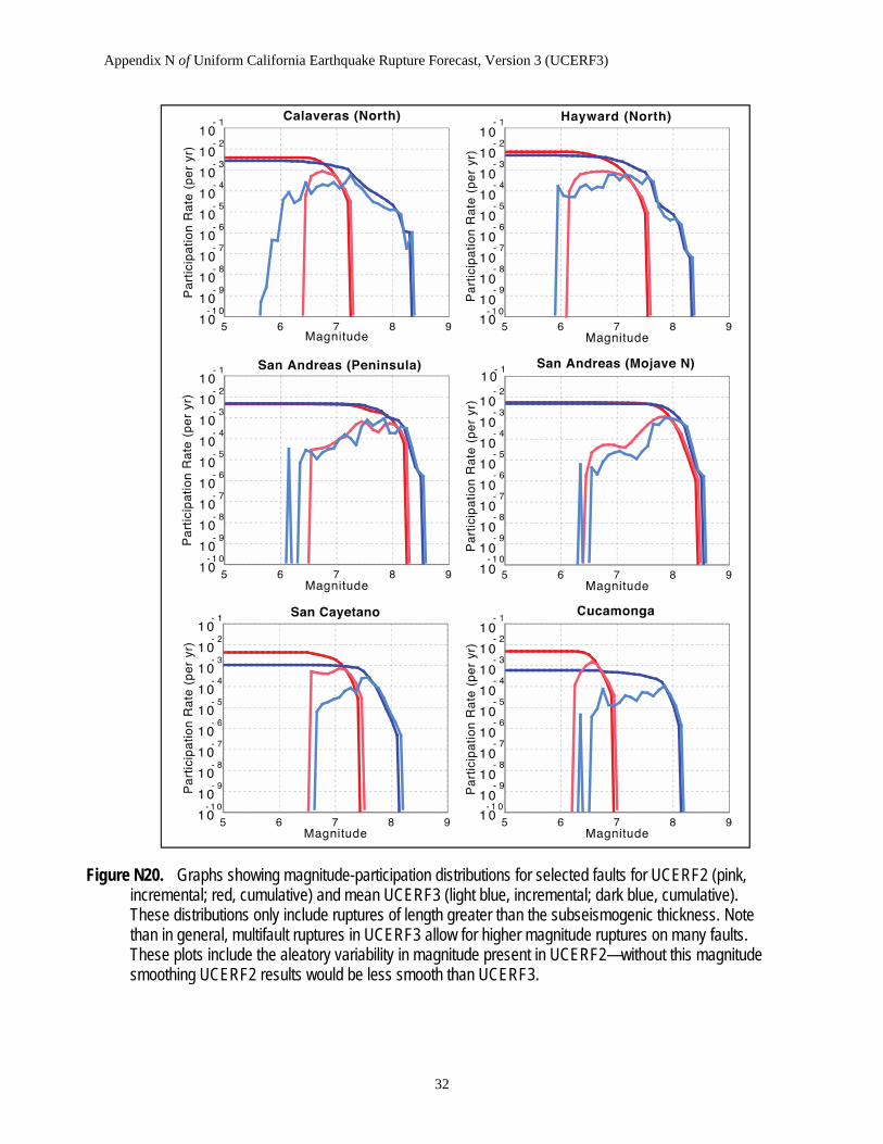
Of particular importance for seismic hazard is the distribution of event sizes at a point. Magnitude-frequency participation distributions for selected faults of interest are shown in figure N20. The increased connectivity of the fault system allowed in UCERF3 is readily apparent in these examples; multi-fault ruptures allow for larger magnitudes on many major faults. Further visualizations of ruptures including the Hayward North and SAF Mojave South fault sections are shown in figures N21 and N22.


32

Figure N20. Graphs showing magnitude-participation distributions for selected faults for UCERF2 (pink, incremental; red, cumulative) and mean UCERF3 (light blue, incremental; dark blue, cumulative). These distributions only include ruptures of length greater than the subseismogenic thickness. Note than in general, multifault ruptures in UCERF3 allow for higher magnitude ruptures on many faults. These plots include the aleatory variability in magnitude present in UCERF2—without this magnitude smoothing UCERF2 results would be less smooth than UCERF3.


33

Figure N21. Visualization (A) and map (B) of ruptures involving the Hayward South fault section. Faults that rupture with the Hayward South are colored on the map by the total rate those ruptures occur. In the visualization of those ruptures, the trace of ruptures is plotted floating above the fault trace, ordered and colored by rate. Segmentation can be seen as common stopping points for ruptures; this segmentation is not prescribed explicitly by the model, but rather is a consequence of the data and constraints.

Figure N22. Visualization of ruptures involving the Mojave South fault section of the San Andreas Fault. (A) Map showing faults that rupture with any of the subsections of Mojave South, colored by the total rate those ruptures occur. (B) A visualization of those ruptures; the trace of ruptures is plotted floating above the fault trace, ordered and colored by rate. Common stopping points for these ruptures include the San Andreas Fault Creeping section, and the San Jacinto/SAF boundary.


34

Timing Correlations Between Neighboring Paleoseismic Sites The UCERF3 models are directly constrained to fit paleoseismic event rate and mean slip

data at points along faults. One set of data that is not directly included, however, is the correlation of event dates between adjacent paleoseismic sites. This is a nonlinear constraint that is difficult to include directly in the inversion; however, we can check to see how well the inversion matches this independent set of data.

Figure N23. Plot showing comparison of timing correlations between paleoseismic sites and the rate these sites rupture together in UCERF2 and UCERF3 along the Southern San Andreas Fault. As discussed in the text, UCERF3 matches the correlation data slightly better than UCERF2, on average, even though these data are not directly constraining the inversion.

We compare the fraction of events that are correlated between paleoseismic sites (the total number of events for which the age probability distributions are consistent between sites divided by the total number of events) with the fraction of the time those fault subsections rupture together (in paleosiesmically visible ruptures) in the inversion. This comparison for the Southern San Andreas Fault is shown in figure N23. The 95-percent probability bounds on the data show sampling error only, given the number of events observed; they do not take into account, for example, the probability that events closely spaced in time could have consistent ages. For this fault, UCERF2 and UCERF3 each fall outside of the 95-percent confidence bounds of the data for one site pair. However, they are each below the bounds, which may be acceptable because not all timing correlations in the paleoseismic data necessarily represent the same event. Some correlated events could be separate events beyond the time resolution of the paleoseismic data. Being above the 95-percent confidence bounds is more problematic—UCERF2 falls above the bounds at one site on the Northern San Andreas Fault and both UCERF2 and UCERF3 are


35

above the bounds at one site on the San Jacinto Fault, although UCERF2 misses the data by more at this site.

In conclusion, Mean UCERF3 fits the paleoseismic timing correlations slightly better than UCERF2, although this may not be true for every individual branch of UCERF3. The performance of UCERF3 is surprisingly good, given that it outperforms UCERF2 without including these data directly as a constraint.

Misfits for Individual Logic-Tree Branches We can compute misfits for each constraint of each logic tree branch (as well as a total

misfit that is a weighted average of these); examination of these misfits allows us to determine which branch choices are “preferred” by the inversion in the sense that the misfits are smaller. In general, branches that have lower misfit are branches where the total moment balancing is less constrained. For example, better misfits are typically obtained with the UCERF3 spatial seismicity distribution, which leaves more available moment on the faults; similarly, a higher total seismicity rate for the region (which, again, leaves more available moment to distribute on the faults) gives lower misfits. The Average Block Model (ABM) (appendix C, this report) typically gives the worst misfits among the deformation models; it has the largest target moment on the faults (and this makes moment balancing more constrained because UCERF3 models underpredict the total on-fault moment).

These misfits also presumably include information about correlations between logic tree branches. For example, one scaling relation (that, say, tends to give high slips) may work poorly with a deformation model that has high slip rates but work well with a deformation model that gives lower slip rates. Logic trees employed in probabilistic seismic hazard analysis typically do not have a mechanism to include correlations between branches; that is, the choice on one level of the logic tree is independent of the choice at another level. One could devise, however, a weighting scheme that uses the total misfit for each branch of the logic tree as a likelihood function to update the prior weights determined from expert opinion using Bayes’ rule. In this way, single paths through the logic tree that do not fit the data as well could be weighted lower.

We are not currently employing such a Bayesian scheme in UCERF3; we are using only a priori weights determined by expert opinion. Branch misfits do not necessarily represent model likelihood; for example, the branches using uniform slip along a rupture outperform those branches that use a tapered slip distribution. This is despite the fact that the tapered distribution far better reflects the average slip distribution of ruptures seen in the data. The uniform distribution of slip has lower misfits because it makes it easier to fit the step-like changes in slip rates along faults. These slip-rate changes are probably not physical either; they are simply a modeling simplification. But in this case, the inversion misfits are not telling us that the uniform slip distribution is correct, just that it is more consistent with other data simplifications in the model.

Links to More Results Many more plots than it is feasible to present here have been generated and are available

as supplementary material. These plots include magnitude distributions on every fault in the model, paleoseismic fits for all faults with paleoseismic data, and hazard results using a range of metrics. This material is available in supplementary files attached to this report online.


36

Concluding Remarks The inversion approach developed for the UCERF3 project relies on data inputs and

models from many other project tasks to determine the rates of on-fault ruptures. Many of these inputs will be uncertain and subject to debate. However, it is important to note that all these uncertainties existed in the old methodology for determining rupture rates as well. The inversion methodology described here eliminates the need for prescriptive assignment of rupture rates. It provides a means to easily update the model as new data becomes available. Importantly, the inversion methodology provides a mechanism to simultaneously constrain the model by multiple datasets concurrently. This was lacking in UCERF2—expert opinion did not simultaneously satisfy slip rates and event rates, and the magnitude distribution of the final model was inconsistent with the observed distribution and the well-supported assumption that the regional MFD will be characterized by a Gutenberg-Richter distribution (appendix L, this report). The inversion allows all these constraints to be satisfied to the extent that they are compatible.

The inversion can also be used as a tool to determine when a set of constraints is not compatible. Earlier inversion models, for example, showed that some deformation models (since updated) were not compatible with historical seismicity rates and the assumption of full coupling on the faults. This led to significant revisions of the deformation models, which brought the inversion ingredients into better alignment. The Gutenberg-Richter branch of the model also demonstrates incompatibilities with model ingredients: on-fault deformation model moments, if fully seismic, are not compatible with low historical seismicity rates given the current connectivity of the model, if we assume an on-fault b-value of 1.0 and assume that 58 percent of seismicity is on the faults (see main text of this report). These branches have been given zero weight in UCERF3 because of the low on-fault coupling coefficients that they imply. One way these incompatibilities could be mitigated is with increased connectivity, which would allow more on-fault moment in the model.

The degree to which modeled fault connectivity affects the final model results is quite significant. There are several aspects of the model that suggest that the connectivity assumed in UCERF3, while greater than connectivity assumed in past models, is an underestimate of the true connectivity in nature. As described in the “Setting up the Inversion: Data and Constraints” section, the rates of multi-fault ruptures in the model underpredict their observed rates. Furthermore, many of the misfits in the model could be improved if maximum magnitudes were higher, particularly on secondary faults. For example, more moderate-sized earthquakes on the Southern San Andreas would bring the synthetic paleoseismic rates closer to the observed rates. However, the regional magnitude distribution constraint only allows a finite budget of moderate earthquakes, and many are instead used to match slip rates on faults that cannot rupture in large, M~8 earthquakes as a result of the connectivity assumptions.

Because of the global nature of the applied constraints, all aspects of the model are linked; hence, changing the data or parameterization for one particular fault can affect the solution elsewhere in the fault system. This can be problematic, in that errors in the inputs can propagate spatially; however, the flexible, system-level UCERF3 approach allows for sensitivity to connectivity and other model assumptions to be explored. This leaves many exciting avenues for future work, such as investigating trade-offs in the model and testing new hypotheses of earthquake recurrence.


37

Acknowledgments Computation for the work described in this manuscript was supported by the University

of Southern California Center for High-Performance Computing and Communications (http://www.usc.edu/hpcc). The authors also acknowledge the Texas Advanced Computing Center (TACC) at The University of Texas at Austin and the Extreme Science and Engineering Discovery Environment (XSEDE) for providing high-performance computing resources under XSEDE grant number TG-MCA03S012. We are grateful for helpful reviews from Tom Jordan, Art Frankel, Mark Stirling, Karen Felzer, and Sue Hough.

References Andrews, D.J., and Schwerer, E., 2000, Probability of rupture of multiple fault segments:

Bulletin of the Seismological Society of America, v. 90, no. 6, p. 1498–1506, doi:10.1785/0119990163.

Arrowsmith, R., McNally, K., and Davis, J., 1997, Potential for earthquake rupture and M7 earthquakes along the Parkfield, Cholame, and Carrizo segments of the San Andreas Fault: Seismological Research Letters, v. 68, no. 6, p. 902–916, doi:10.1785/gssrl.68.6.902.

Bakun, W.H., and Lindh, A.G., 1985, The Parkfield, California earthquake prediction experiment: Science, v. 229, p. 619–624.

Custódio, S., and Archuleta, R.J., 2007, Parkfield earthquakes—characteristic or complementary?: Journal of Geophysical Research, v. 112, no. B05310, doi:10.1029/2006JB004617.

Field, E.H., and Page, M.T., 2011, Estimating earthquake-rupture rates on a fault or fault system: Bulletin of the Seismological Society of America, v. 101, no. 1, p. 79–92, doi:10.1785/0120100004.

Geman, S., and Geman, D., 1984, Stochastic relaxation, Gibbs distributions, and the Bayesian restoration of images: IEEE Transactions on Pattern Analysis and Machine Intelligence, no. 6, p. 721–741, doi:10.1109/TPAMI.1984.4767596.

Granville, V., Krivanek, M., and Rasson, J.P., 1994, Simulated annealing—A proof of convergence: IEEE Transactions on Pattern Analysis and Machine Intelligence, v. 16, no. 6, p. 652–656, doi:10.1109/34.295910.

Gutenberg, B., and Richter, C.F., 1944, Frequency of earthquakes in California: Bulletin of the Seismological Society of America, v. 34, p. 185–188.

Hanks, T.C., and Bakun, W.H., 2008, M-log A observations of recent large earthquakes: Bulletin of the Seismological Society of America, v. 98, p. 490.

Holland, J.H., 1975, Adaptation in natural and artificial systems—An introductory analysis with applications to biology, control, and artificial intelligence: Ann Arbor, Michigan, University of Michigan Press, 211 p.

Ingber, L., 1989, Very fast simulated re-annealing: Mathematical and Computer Modeling, v. 12, no. 8, p. 967–973, doi:10.1016/0895-7177(89)90202-1.

Kirkpatrick, S.C., Gelatt, D., and Vecchi, M.P., 1983, Optimization by simulated annealing: Science, v. 220, p. 671–680.

Schwartz, D.P., and Coppersmith, K.J., 1984, Fault behavior and characteristic earthquakes—examples from the Wasatch and San Andreas fault zones: Journal of Geophysical Research, v. 89, no. 5, p. 681–698.

http://www.usc.edu/hpcc

http://en.wikipedia.org/wiki/Digital_object_identifier

http://www.sciencedirect.com/science/journal/08957177


38

Shaw, B.E., 2009, Constant stress drop from small to great earthquakes in magnitude-area scaling: Bulletin of the Seismological Society of America, v. 99, p. 871, doi:10.1785/0120080006.

Szu, H., and Hartley, R., 1987, Fast simulated annealing: Physics Letters A, v. 122, nos. 3–4, p. 157–162, doi:10.1016/0375-9601(87)90796-1.

Titus, S.J., DeMets, C., and Tikoff, B., 2006, Thirty five year creep rates for the creeping segment of the San Andreas fault and the effects of the 2004 Parkfield earthquake—constraints from alignment arrays, continuous global positioning system, and creepmeters: Bulletin of the Seismological Society of America, v. 96, no. 4B, p. S250–S268, doi:10.1785/0120050811.

Wesnousky, S.G., 2008, Displacement and geometrical characteristics of earthquake surface ruptures—Issues and implications for seismic-hazard analysis and the process of earthquake rupture: Bulletin of the Seismological Society of America, v. 98, no. 4, p. 1609–1632, doi:10.1785/0120070111.

Wesnousky, S.G., Scholz, C.H., Shimazaki, K., and Matsuda, T., 1983, Earthquake frequency distribution and the mechanics of faulting: Journal of Geophysical Research, v. 88, p. 9331–9340.

Working Group on California Earthquake Probabilities, 1988, Probabilities of large earthquakes occurring in California on the San Andreas fault: U.S. Geological Survey Open-File Report, p. 62.

Working Group on California Earthquake Probabilities, 2003, Earthquake probabilities in the San Francisco Bay region—2002–2031: U.S. Geological Survey Open-File Report 2003–214.

Working Group on California Earthquake Probabilities, 2007, The uniform California earthquake rupture forecast—version 2 (UCERF2): U.S. Geological Survey Open-File Report 2007-1437.

Date post:	21-Dec-2021
Category:	Documents
Upload:	others
View:	1 times
Download:	0 times

Appendix N—Grand Inversion Implementation and Testing

Documents