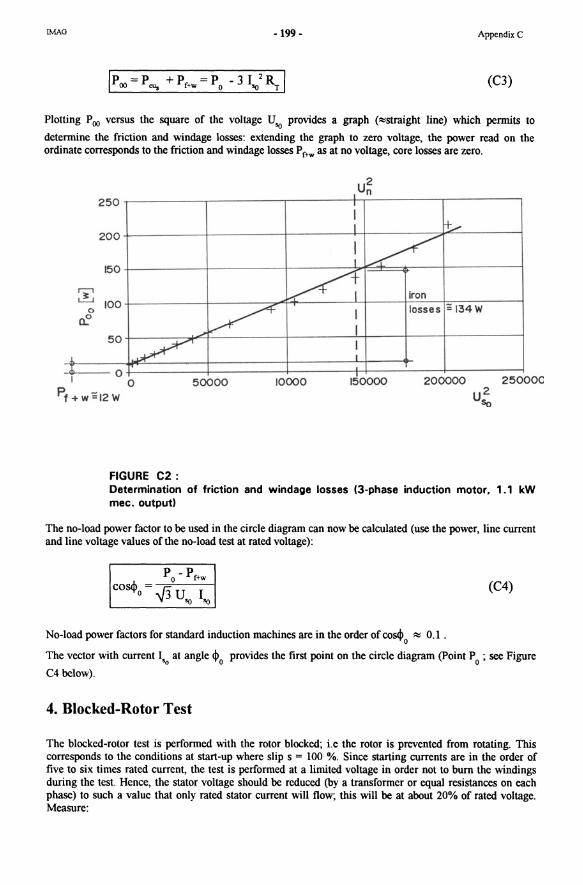
APPENDIXA BASIC THEORY OF ELECTRICAL ENGINEERING 1. INTRODUCTION978-3-663-14… · ·...

!MAG -115 - AppendixA

APPENDIXA

BASIC THEORY OF ELECTRICAL ENGINEERING

1. INTRODUCTION

1.1 Electrical Circuit Electric CUTTent consists of the f10w of electrons in conductors. The energy of this f10w can be converted into motion (motors) or heat (Iamps, boilers). The three basic parts of an electrical circuit are the source, the conductor and the load. An electrical circuit resembles in many ways a hydraulic pipeline system.

T

Volve

FIGUREAl : The electrical circuit and its hydraulic equivalent

1.2 Volta ge

Turbine

~pressure -----+ dlfference

Flow Meter

The electrons in the conductors move only as long as there is a source of electrical pressure available. Electrical pressure, known as voltage, is obtained from batteries, generators or photoelcctric cclls (which make up solar panels). Voltage is similar to the pressure difIerence (.!lp) in the hydraulic system measured with a manometer.

Symbol for Voltage: U Unit: Volt (V)

Voltage is measured by means of a VOLTMETER which always measures the difIerence of electrical pressure between two points of an electrical circuit, Le. the voltmeter is connected across (in parallel with) the source or the load.

The voltmeter is an instrument with a low consumption, or in engineering terms, with a high impedance (high resistance to the f10w of elcctrons, so that the electrical pressure difIerence is not discharged through the voltmeter - see Figure Al above).

1.3 Current Applying voltage (pressure difIerence) to an electrical circuit, CUTTent f10ws in the direction of the pressure gradient. CUTTent is the charge (charged electrons) f10wing through a conductor per unit time (second) and comparable to the discharge (m3/s) in the hydraulic circuit.

Symbol for Current: I Unit: Ampere (A)

The CUTTent is measured by means of an AMMETER connected in series (in-line) between the source and the load; Le. the CUTTent f10ws through it like in an orifice-plate f10w meter in the hydraulic system of Figure Al.


The ammeter is an instrument with a low resistance to the flow of electrons (in engineering terms: low impedance). So the loss ofpressure (voltage drop) across the ammeter is small. Note that the current in a circuit without parallel conductors or loads remains constant throughout the circuit.

1.4 Effects of Current Flow Electric current flowing through loads produces the following effects which are used in various applications:

- thermal (beat): heating devices (boiler, tea kettle), tungsten lamps (the metaI filament in a light bulb glowing white and giving heat and light, but does not burn due to the absence of oxygen), industrial fumaces, electric welding;

- magnetic: motors, relays, beils, electromagnets, measuring instruments (see also Seetion 3)

- chemical: electrolysis (separation of substances into its chemical components), accumuJators, galvanization;

- luminescent: fluorescent tubes.

1.5 Power Power is the rate of work done or energy supplied/consumed per unit time. One Watt is the power used when one Ampere is forced through a circuit by apressure (voltage) of one Volt.

Symbol of power: P Unit: Watt (W)

Energy / unit time = Joule (J = W·s) / second = Watt

In a DC (direct current) circuit the power is always

Ip = Volt * Ampere = U I I (Al)

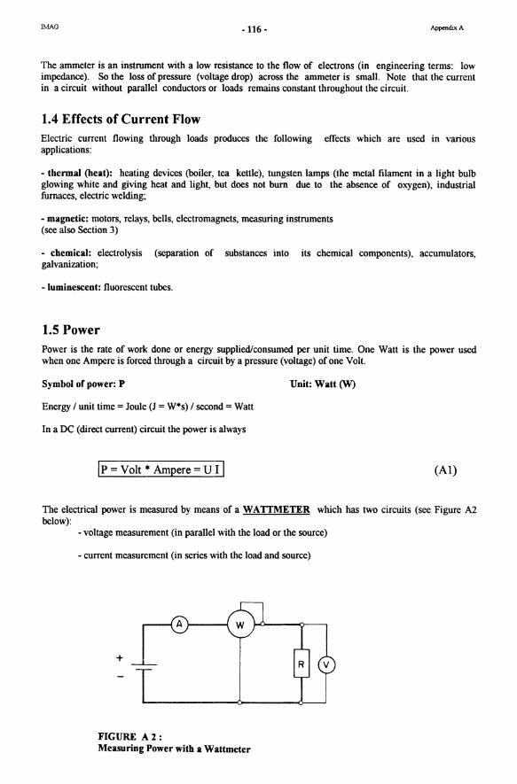
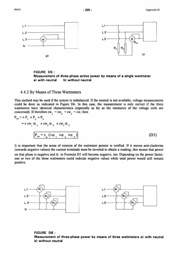
Tbe electrical power is measured by means of a WATTMETER which has two circuits (see Figure Al below):

- voltage measurement (in parallel with the load or the source)

- current measurement (in series with the load and source)

+

FIGURE A2: Measuring Power with a Wattmeter


2. DIRECT CURRENT (DC) If current does not change its direction of flow, it is ca1led direct current and the symbol is:

= or -- (DC)

If a constant voltage is connected to the terminals of a resistor(lamp, heating device), direct current (I ) will flow through that resistor.

Sources of direct current are:

- cells (batteries) and accumulators - generators with commutator (commutator = mechanica1 device rectifying the direction of a current) - diode bridge rectifier (diode = semi-conductor element

which lets only one direction of current pass; thus an altemating current can be rectified (made direct current) - thyristor converters (similar to diode but with regulation)

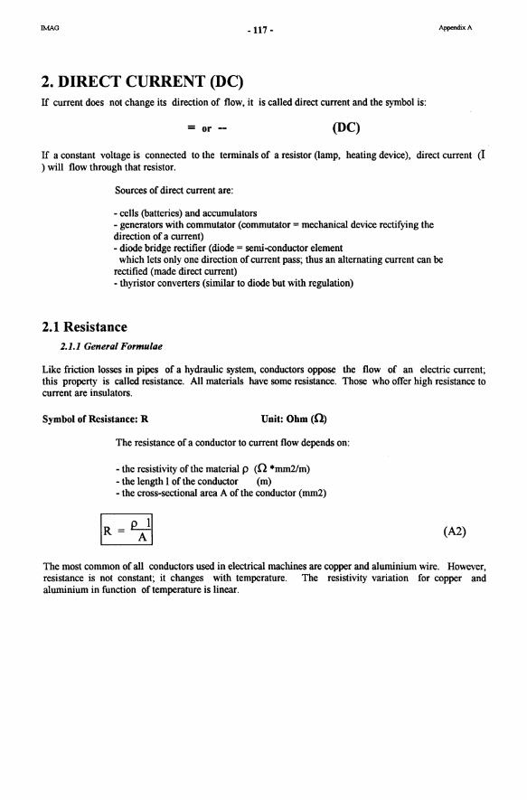
2.1 Resistance 2.1.1 General Formulae

Like friction losses in pipes of a hydraulic system, conductors oppose the flow of an electric current; this property is ca1led resistance. All materials have some resistance. Those who offer high resistance to current are insulators.

Symbol or Resistance: R Unit: Ohm (0)

The resistance of a conductor to current flow depends on:

- the resistivity ofthe material p (0 "'mrn2/m) - the length I ofthe conductor (m) - the cross-sectional area A ofthe conductor (rnm2)

(A2)

The most common of all conductors used in electrical machines are copper and aluminium wire. However, resistance is not constant; it changes with temperature. The resistivity variation for copper and aluminium in function oftemperature is linear.

IMAG -118 -

resistivity 8

------235

FIGURE A3: Resistivity of cop per as a function of temperature

For copper, the following formula applies:

T-T PT = PTo (1 + 235 + T )

o

(for aluminium, replace the value of 235 with 250)

PT = final resistivity in n mm2/m

PTo = initial resistivity in n *mm2/m

T = final tempcrature in 0 Celsius

To = initial temperature in 0 Celsius

AppendixA

T temperature T

(A3)

As initial conditions, the resistivity at To = 200 C is usually assumed; the resistivity of copper and aluminium for this temperature are:

- copper: P 200 C = 0.0175 n *mm2/m

- aluminium: P 200 C = 0.03 n *mm2/m

Since resistance is proportional to P , the above formula applies also for resistance at tempcrature T :

T - T RT = RTo ( 1 + 235 + T) für copper

o (A4)

2.1.2 Ohm's Law

There is adefinite relationship between the voltage U aeross a resistance and the current flowing through it, known as Ohm's Law:

IU=RII where U = Voltage across the resistance in Volt

I = Current in Amperes R = Resistance in Ohms

2.1.3 Puwer Losses - Joule's Law

(A5)

When a current flows through a resistance R, energy is lost in the form of heat (thermal effect). Power was defined as energy consumed per unit time and, in the case of DC circuits, is equivalent to voltage times


current, P = U * I. These energy losses cause a decrease ofthe driving force (= voltage) ofthe electrical

current in a circuit, known as voltage drop. Applying Ohm's law U = R * I ,the amount of power lost through a resistance R can be calculated as folIows:

Ip = U land U = R I (A6) thus

Ip = R I 21 PowerPinWatt(W)

Joule's Law

d· . I 2 The correspon mg energy lS: E = P t = U t = R I t

2.1.4 Connection 0/ Resistances

• Scrics Connection

(A7)

(Ws)

So far, only one resistance has been considered. In most practica1 applications circuits consist of several devices, e.g. a lamp and its fecding conductors represent both resistors. In aseries circuit the devices are connectcd one after the other along the conductor. Apparently, there is only one path for the current and the same current f10ws through each resistor.

1 1 R1

U R2 U2 R3

I U3 I

FIGURE A4: Series Connection of Resistances

The total voltage U across the terminals of the source is equal to the sum of the voltage drops of each resistor:

U= U1 + U2 + U3 + ... + Un applyingOhm'sLawU=RI

U = R1 I + R2 I + R3 I + ... + Rn I = R I

Total circuit resistance or equivalent resistance R (in series connection)

(A8)


• Parallel Connection

A parallel circuit offers aseparate path for the current to each load.

I I

u u

FIGURE A5: ParaIlel Connection or Resistances

Each resistor is individually connected to the rnain source and therefore, each resistor operates under the same voltage as the source:

In a parallel circuit the resistors operate independently of one another and take current according to their

resistances. However, the total current of all resistances is equaI to the current 1 supplied by source:

1 =1 1 +1 2 +1 3 + ... +l n

Applying Ohm's Law 1 = UIR gives the total circuit or equivalent resistance R (for parallel connection):

(A9)

Example 1:

The wiring system of a house consists of the following devices:

- 31amps in parallel (Rl: 25 W at 24 V; R2: 10 W at 24 V; R3: 15 W at 24 V)

- 2 lamps in series (R4 = R5: 15 Wat 12 V)

There is a 12 Volt DC supply at a distance of 200 m from the house. Copper wiring is used with a cross-sectional area of 1.5 mm2 (wiring inside the house between devices can be neglected). Calculate the total current in the supply line and the power requirement of the house if all devices are switched on simultaneously. Comment on the voltage across the lamps as compared to their ratings. Comment also on the size of the selected conductor (see Appendix BI for standard wire sizes and maximum current). The

ambient temperature is 35 0 Celsius.

Solution (see at the end of Appendix A)

IMAG -121 - AppendixA

2.2 Capacitance of Capacitors

1.1.1 General

Capacitors are a means to store electrical energy. As shown in section 1.2 above voltage (electrical pressure) is created by separating electric charge (electrons) into two different parts where one (the negative pole) apparently has a surplus of electrons and the other (the positive pole) has a lack of electrons. If connected, the two parts will level out their different charges and a CUTTent (electrons) will flow from one pole to the other providing electric CUTTent to drive devices. All sources of electrical energy work on this principle. Consider two metal plates placed at some distance from each other and supplied by DC voltage. The same separation of charge as in the source will be observed on the two plates: positive electric charge will accumulate on one plate and negative charge on the other. These two plates constitute an elcmentary capacitor.

+ + +

FIGURE A6: Elementary Capacitor

1.1.1 CapaciJance

Symbol: C Unit: Farad F = Ampere*secondNolt

The quantity of electricity (charges) which a capacitor can store if supplied by a certain voltage depends only on the size (area of plates, distance in between) and the physical properties (filling of the capacitor) and is called capacitance C of the capacitor.

C=Q/U where Q = quantity of electric charges in Ampere*seconds stored

In practice, capacitors have very low capacitance; it is therefore more convenient to use Microfarad (10-6 -9

Farad) or Picofarad (10 Farad).

1.2.3 Variation ofCurrent und Voltage

Charging and discharging of capacitors is not an instantaneous process, it takes some time until the charges (electrons) have moved to or from the capacitor. At the beginning of the charging process a CUTTent flow is observed while the CUTTe nt will stop as soon as the voltage across the capacitor has reached the same value as the source voltage.

IMAG

Source

FIGUREA 7:

+

a

+

+ ---0

b

+ --0

-122 -

I

I

Charging and Discharging a Capacitor

current i

charging )

CT

1 =0

charged C

discharging C

1=0

discharged C

+

T

AppendixA

Applying a DC voltage to a circuit with a resistance R and a capacitance C (Fig. A 8a), it can be shown (using Ohm's law) that the initial current i = U 0 / R will flow through R, where U 0 is the constant source

voltage. Since this initial flow of current has created a voltage (charge) across the capacitor, the voltage drop (pressure to initiate flow) across the resistance is now lower than U 0' hence current i in the circuit

will take a lower value. Thus neither i nor u take constant values during the charging process and we can write (note, smailletters are used for current and voltage which vary in time):

i = C • .1u / .1t

The capacitor voltage increases in the same manner as the voltage drop across the resistance and therefore current in the circuit decreases; this is shown graphica\ly in Figure A 8b.

!MAG -123- AppendixA

® tCharging ~

.diSCharging R

C

3't" t -~

3" 0

to 1'1: 2'1: 3'1:' I

't' ~ L 1 I Charging Discharging I ' ... to

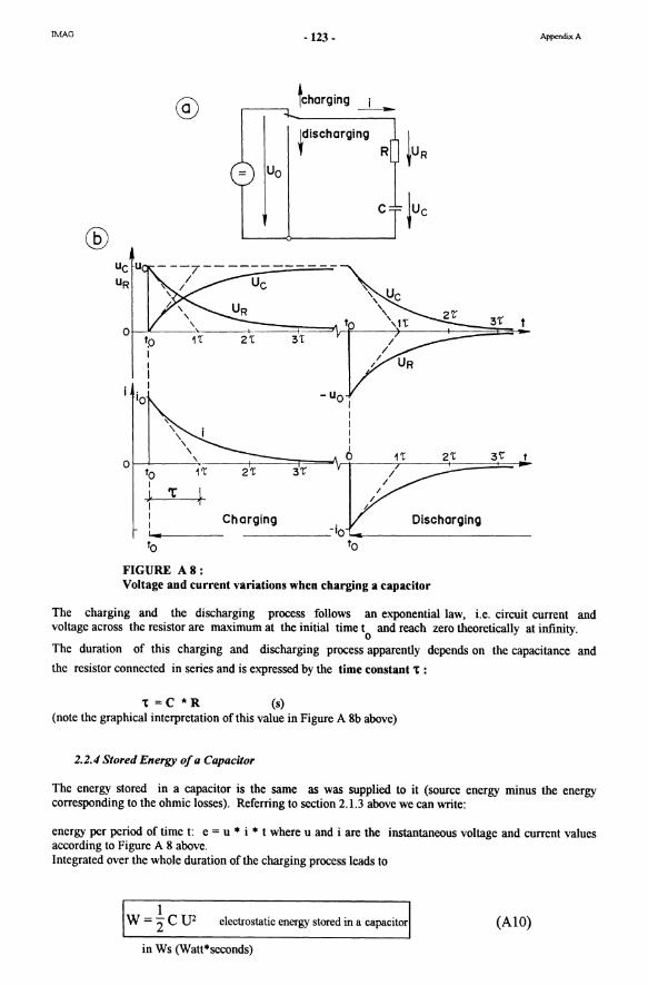
FlGURE AB: Voltage and current variations when charging a capacitor

Tbe charging and the discharging process follows an exponential law, i.e. circuit current and voltage across the resistor are maximum at the initial time t and reach zero theoretically at infinity.

o Tbe duration of this charging and discharging process apparently depends on the capacitance and

the resistor connected in series and is expressed by the time constant 't :

't = C * R (5) (note the graphical interpretation ofthis value in Figure A 8b above)

2.2.4 Stored Energy 0/ a Capacitor

Tbe energy stored in a capacitor is the same as was supplied to it (source energy minus the energy corresponding to the ohmic losses). Referring to section 2.1.3 above we can write:

energy per period of time t: e = u * i * t where u and i are the instantaneous voltage and current values according to Figure A 8 above. Integrated over the whole duration ofthe charging process leads to

1 W=-ClJ2 2 electrostatic energy stored in a capacitor

in Ws (Watt*seconds)

(AIO)


Example 2: A photo-flash requires 100 Ws at a voltage of 800 V to produce a bright flash. Calcu1ate the size of the capacitor required to store this energy. Determine also the resistor required to be connected in series with the capacitor if the current from a 1.5 V battery should not exceed 0.1 A when charging the capacitor.

Solution see at the end of Appendix A.

2.2.5 Connection ofCapacitors

• Connection in series

Figure A 9 shows several capacitors connected in series.

Cn C

.. - .. U UC2 UCn

.. U

FIGURE A9: Capacitors in series

The total voltage U is equal to the sum ofthe individual voltage across each capacitor: U = U I + U2 + U3

+ ... +U n

Since there is only one path offered for the current to flow, I must be the same for all capacitors. From section 2.2.3 above we know that the current is directly proportional to the capacitance and the change of

voltage through each capacitor: I = C * L\U / L\t. Hence, the product C * L\U must be constant for all capacitors:

I = Cl L\U1/L\t = C2 L\UiL\t = C3 L\UiL\t = Cn L\ UrlL\t = C L\U/L\t where C is the equivalent capacitor

of the serie.

since I I C = L\U I L\t = lIL\t(L\UI + L\U2 + L\U3 + ... + L\Un) and L\U = L\t I IC we can write:

I I C = I I Cl + I I C2 + I I C3 + ... + I I Cn

Equivalent Capacitor C (for series connection)

C= 1 lICI + lIC2 + lIC3 + ... lICn

(All)

IfCI = C2 = C3 = Cn the equivalent capacitorbecomes C = CII n


• Connection in parallel

Figure A 10 below shows several capacitors connected in parallel.

I a .}" ul

I C1 I C2

C~ C2 .JC

"

b

FIGUREA 10: Capacitors in parallel

Voltage across each individual capacitor is equal to the voltage of the DC source. The total current I is the sum of the individual currents flowing through each capacitor (note that current (electrons) actually cannot pass the capacitor; they accumulate on one plate of the capacitor whereas on the other a lack of electrons is created because on the latter, they have moved towards the source ofthe circuit.) Applying the same relationship as for series connection above, the equivalent capacitor for parallel connection becomes:

(A12)

Example 3: The capacitor chosen for the photo-flash in Example 2 is to be replaced by two capacitors of which the second is twice as big as the first one. Which connection is to be preferred if the capacitors should be as small as possible?


3. MAGNETISM - ELECTROMAGNETISM

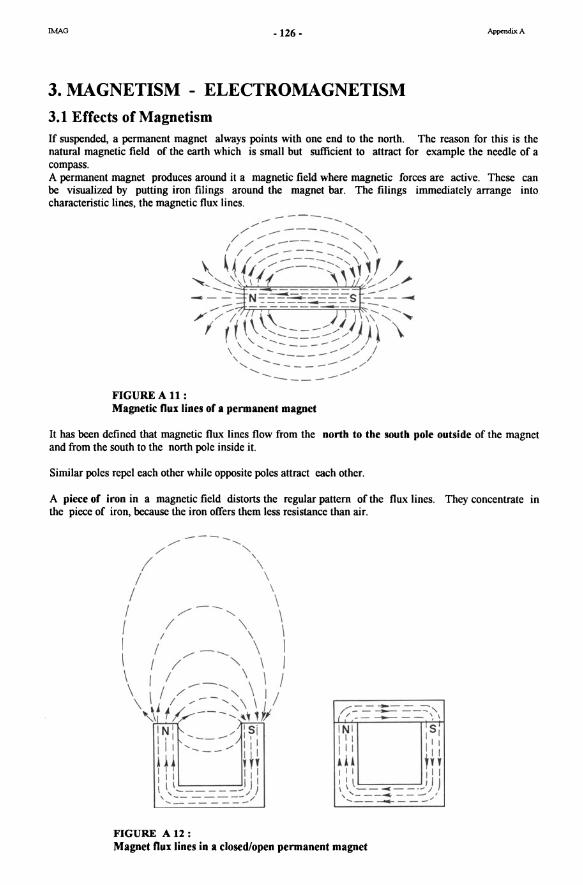
3.1 Effects of Magnetism If suspended, a permanent magnet always points with one end to the north. Tbe reason for this is the natural magnetic field of the earth which is smaIl but sufficient to attract for example the needle of a compass. A permanent magnet produces around it a magnetic field where magnetic forces are active. These can be visuaIized by putting iron filings around the magnet bar. Tbe filings immediately arrange into characteristic lines, the magnetic flux lines. -----

----

--------FIGUREAll : Magnetic flux Iines of a permanent magnet

It has been defined that magnetic flux lines flow from the Dortb to the soutb pole outside of the magnet and from the south to the north pole inside it.

Similar poles repel each other while opposite poles attract each other.

A piece of iron in a magnetic field distorts the regular pattern ofthe flux lines. Tbey concentrate in the piece of iron, because the iron offers them less resistance than air.

/::.:..::.=-~--" {'------ '.' I N I 5 1 11 1 1 : 1 I I 111

.Ai 'U I 11 11 I 1 1 \ iI } \ \ - . ~ I ,..:-.:.=~=. --=--: .....

FIGURE All: Magnet flux lines in a c1osed/open permanent magnet


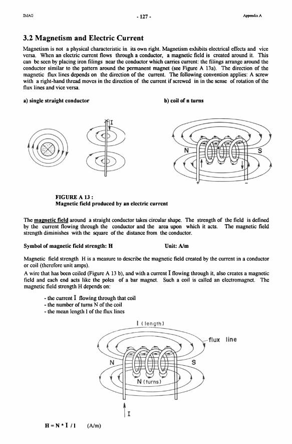
3.2 Magnetism and Electric Current Magnetism is not a physical charactcristic in its own right. Magnetism exhibits electrical effects and vice versa. When an electric current flows through a conductor, a magnetic field is created around it. This can be seen by placing iron filings near the conductor which carries current: the filings arrange around the conductor similar to the pattern around the pennanent magnet (see Figure A Ba). Tbe direction of the magnetic flux lines depends on the direction of the current. Tbe following convention applies: A screw with a right-hand thread moves in the direction of the current if screwed in in the sense of rotation of the flux lines and vice versa.

a) single straight conductor b) coil of n turns

-tr--- - ---::

FIGUREA 13: Magnetic fjeld produced by an electric current

The magnetic fjeld around a straight conductor takes circular shape. Tbe strength of the field is defined by the current flowing through the conductor and the area upon which it acts. Tbe magnetic field strength diminishes with the square ofthe distance from the conductor.

Symbol of magnetic fjeld strengtb: H Unit: Alm

Magnetic field strength H is a measure to describe the magnetic field created by the current in a conductor or coil (thcrefore unit amps). A wire that has been coiled (Figure A 13 b), and with a current I flowing through it, also creates a magnetic field and each end acts like the poles of a bar magnet. Such a coil is called an electromagnet. Tbe magnetic field strength H depends on:

- the current I flowing through that coil - the number of turns N of the coil - the mean length I of the flux lines

Il length )

line

H=N *1/1 (Nm)


Tbe strength of the field varies both in direction and magnitude: it is highest inside the coil and diminishes quickly outside of the coil due to the variable length of the flux lines. Tbe constant product of

the abovc formula N * I is thcrefore called magnetomotive force or magnetic potential or total

excitation 9. Under its influence, work can be done such as arranging iron filings, turning the needle of a magnet etc.

3.3 Magnetic Flux and Magnetic Flux Density When describing magnetic field strength we looked at the cause of the magnetic field or its potential due to the electric current. Magnetic flux on the other band looks at the potential effect of tbe magnetic field. Tberefore, the magnetic flux lines are considered to carry energy such as the strearn-lines offlowing water. A coil of N turns is wound around an iron core (or other ferromagnetic material, see Figure A 14). When an electric current flows through the coil, magnetic lines of force are produced. All these lines together constitute the magnetic flux.

Symbol of magnetic flux: CI» Unit: Weber (Wb = V*s)

L of oll flux lines" ~

/ ~

/

" . '\

I I I - . ~ i 0) . ~ /i l \

~ I ~ ! I \..._ ._- _....J

/

FIGUREA14 : Magnetic Flux

Magnetic flux per unit area is called magnetic flux density or magnetic induction.

Symbol of magnetic induction: B Unit: Tesla (T = Wb/m2)

(AI3)

3.4 Magnetic Characteristic - Magnetization Curve As shown in Figures A 12 and A 14 above, magnetic flux lines are concentrated in the material which offers little resistance such as in an iron core. For open cylindrical coils filled with air (Figure Al3 b), the flux lines cover a much wider area and the magnetic effect of an electric current is therefore reduced. Tbe magnetic field strength H is related to flux density B as folIows:

(A14)

lMAG -129 - AppcndixA

~ is the product of the permeability in vacuum u and the relative permeability of the material U : o ~

I~ = ~o ~rl Jl = 4*1t *10-7 (V*s/A*m)

o Jlr in air = l.0

(AIS)

Tbe preferred material in magnetic circuits are ferromagnetic ones (= similar to iron). Ferromagnetic are iron, nickel and cobalt and some a1loys of these. Tbe permeability of ferromagnetic material is not constant. Figure A 15 shows the cbaracteristic of a ferromagnetic material in comparison with air.

Induction B ---Wb/m2

IRON

AIR

Magnetic Fleld H [A/mJ

FIGURE A 15: B-B characteristic of iron and air

Above a certain point, the ferromagnetic quaIity seems to be lost and an effect caIled saturation occurs. Tberefore, flux density or induction does no longer increase above a certain point even though the CUTTent in the coil (magnetizing force) is still increasing.

Figure A 16 below shows the complete cbaracteristic of a ferromagnetic material. Complete means here that magnetization is carried througb a complete cycle into negative values (change of direction of CUTTent in the coil). It reveals that the initial curve of magnetization (until saturation) is not retraced when the CUTTent in the coil (and subsequently the magnetizing force H) is decreasing; this effect is caIled hysteresis.

Note that the material, once magnetized, remains magnetic even after the electric CUTTent in the coil has stopped (H = 0). Tbis is called residual magnetism (or remanence Brl and is, for example,

used to create permanent magnets.

!MAG

-H

o

FIGURE A 16:

-130 -

+8 in T

-8

Complete Cbaracteristic of a ferromagnetic material

3.5 Generation of an Electromagnetic Force

AppendixA

A

+ H in A/em

Figure A 13 above has shown that a conductor carrying a cUffent creates a magnetic field of circular shape around it. If another conductor is placed e10se to the first one, the following effects occur:

- two conductors carrying CUTTent in the same direction attract each other (see Figure A 17a);

- two conductors carrying current of opposite direction repel eacb other (see Figure A 17b).

!MAG -131 - AppcndixA

0) b)

- -ottroction repulsion

FIGURE A 17: Interaction of two magnetic fields

Superimposing the magnetic flux lines of the two conductors gives aresultant rnagnetic field with areas of high density and others of low density (see Figure above). A magnetic force acts on either of the two conductors towards the wcaker area of the resultant magnetic field.

Similar effects can be observed when a conductor canying a current I is placed in a rnagnetic field of density B (produced for example by a permanent magnet) and flux Iines perpendicular to the conductor. A force is exerted on the conductor resulting in the displacement ofthe conductor.

!MAG

N

5

FIGUREA18 :

-132 -

I Ind ividual tit>lds Rpsult ing fit>ld

dirt>ct ion of currt>nt

Lt>ft - Hand - Rul p (tor motors)

Force on a conductor in a magnetic field

Appendix A

A qualitative solution of the problem is obtained by superimposing the two magnetic fields; the resultant field shows the areas of high and low density and the direction of the magnetic force on the conductor can be determined. Another qualitative solution is given in Figure A 18 using the "Left-Hand Rule".

Tbe force is proportional to: - the mean value of the magnetic induction B

- the current I flowing through the conductor - the length I of the conductor in the magnetic field.

Ifthe conductor is pemendicular to the magnetic field B:

IF = B * I * 11 (A16)

As can be irnagined, this phenomenon leads to the working principle of the De motor. It will be treated in more details in the next section.


4. INDUCED VOLTAGE

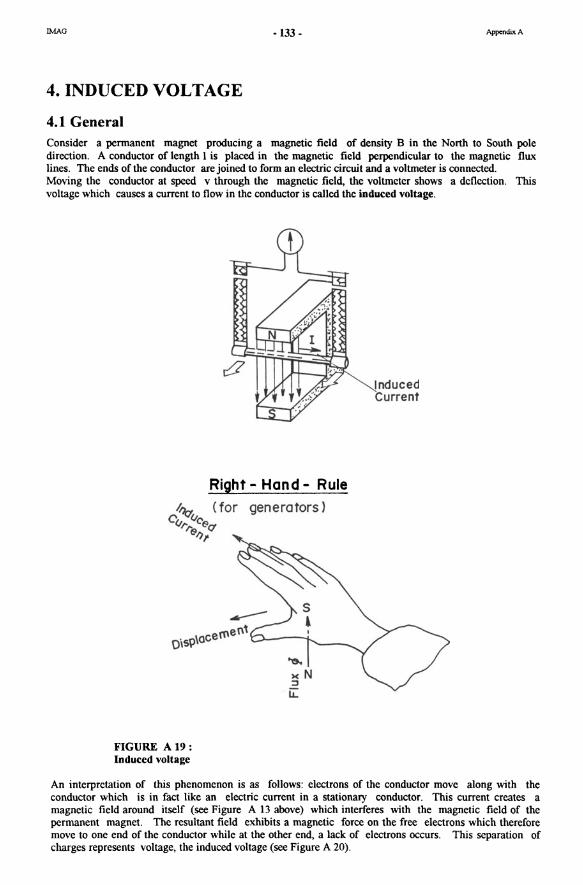
4.1 General Consider a permanent magnet produeing a magnetie field of density B in the North to South pole direction. A conductor of length I is plaeed in the magnetie field perpendieular to the magnetie flux lines. Tbe ends of the conductor are joined to form an electrie eireuit and a voltmeter is connected. Moving the eonduetor at speed v through the magnetie field, the voltmeter shows a defleetion. This voltage which eauses a current to flow in the conduetor is called the induced voltage.

Right - Hand - Rule

~ (for generators) Cf.trr.f.tc@C1

@/}t

FIGURE A 19: Induced voltage

Induced Current

An interpretation of this phenomenon is as folIows: electrons of the eonduetor move along with the eonduetor whieh is in fact like an electrie current in a stationary conduetor. Tbis current ereates a magnetie field around itself (see Figure A 13 above) whieh interferes with the magnetie field of the permanent magnet. Tbe resultant field exhibits a magnetie force on the free eleetrons whieh therefore move to one end of the eonduetor while at the other end, a lack of electrons occurs. This separation of eharges represents voltage, the indueed voltage (see Figure A 20).

!MAG -134 -

FIGURE A20: Interpretation of Induced Voltage

The induced voltage is proportional to : - the magnetic field density B - the conductor speed v - the conductor length I in the magnetic field

Iv = B * 1 * vi (Volt = Volt·s/m2 • m • mls)

AppcndixA

(AI7)

The direction ofthe induced CUTTent generated by the induced voltage (dosed circuit) is defined by the "Right-Hand-Rule" (see Figure AI9). Instead of a single conductor, a coil can be moved through the magnetic field which increases the induced voltage in the coil considerably.

In general, an induced CUTTent can be created either by:

- moving a conductor or coil through a magnetic field or

- cbangiog tbe magnetic flux of tbe fjeld witb time (d«)/dt)

!MAG -135 - Apperu!ixA

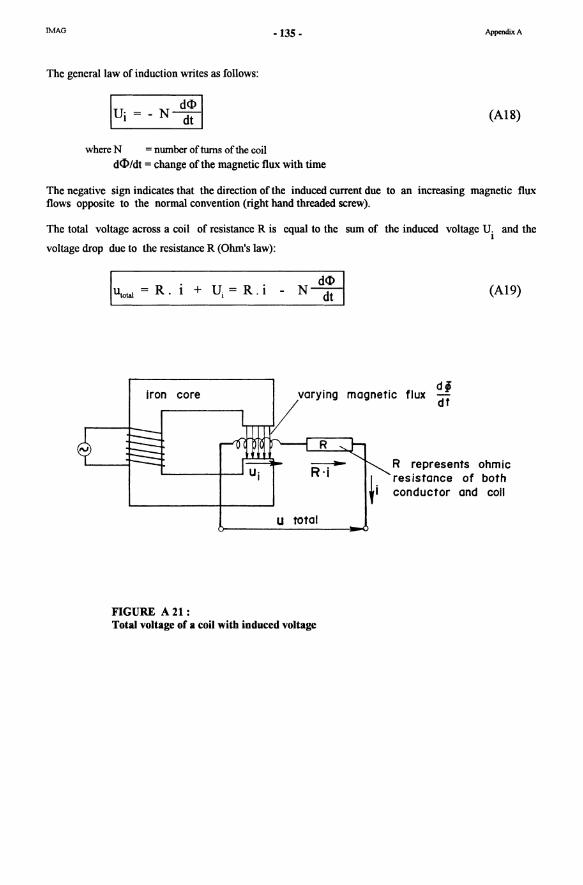
Tbe general law of induction writes as follows:

(AI8)

where N = nurnber ofturns ofthe coil d/dt = change ofthe magnetic flux with time

Tbe negative sign indicates that the direction of the induced current due to an increasing magnetic flux flows opposite to the normal convention (right hand threaded screw).

Tbe total voltage across a coil of resistance R is equal to the surn of the induced voltage Ui and the

voltage drop due to the resistance R (Ohm's law):

R.

iron core

FIGURE A21:

N d: I (AI9)

d, vorying mognetic flux dt

U total

R represents ohmic resistonce of both conductor ond coll

Total voltage of a coil with induced voltage


4.2 Self-Induction To show the phenomenon of self-induction, the following electrical circuit is considered: A DC source is placed in series with a switch, a lamp and a coiL A second lamp is connected in parallel to the source .

U2

Lomp1

u~

r 11---=------' ~ Source

+ -

FIGUREA22 : Self-inductioD

U I

i

.s::. o -"i '"

...--.-p

U2

-----12

time t

On c10sing the circuit, voltage and current are immediately available for lamp I, while lamp 2 lights up only after a certain time. The reason for this lies in the magnetic field created by the current in the coil. Magnetic flux in the coil increases from zero to a maximum value corresponding to the current. This change of flux induces a voltage in the coil itself with a negative sign (see previous section) and thus opposes the voltage ofthe source. This prevents the immediate flow of CUTTent through lamp 2. For large electromagnets, this delay can last up to several minutes (coilslinductances will bc treated in more detail in section 5).

4.3 Transformer Induced Volta ge Consider an iron core with two coils (see Figure A23 below). Coil I is connected to a DC source while the other is an open circuit containing a voltmeter. On c10sing the switch, a magnctic field is created through the iron core as a result of the current in coil I. Due to self-induction, this CUTTent as weIl as the corresponding magnetic field reach only slowly (rapidly at the beginning then with gradually reduced acceleration) their end values.


This gradually changing magnetic field through the iron core induces voltage in coil 2 which has its

maximum value right at the beginning and then reduces to zero at the time when the magnetic flux (<1» of the core remains constant (remember it is only the change ofmagnetic flux which induces voltage). When opening eireuit 1 with the switch S, the same change of magnetic flux occurs as when closing the circuit but the induced voltage in eircuit 2 is now the reverse ofthe former value.

Conclusion: Coils always show a certain degree of inertia to changing conditions. Current and voltage cannot rise or drop sharply in a circuit with a coil.

o

Secondary wlndlng

Switch S

~_source Prlmary wlnding

Circui t

/; i1 ._._.~

U .----.- I ~~--- 1""-

i "'resulting voltage clrcuit CD I ~

-01 voltage U1 due to self-induction

Circuit 2

FIGURE A23: Transformer induced voltage

time t

time t


If the switch S in circuit 1 (containing the primary winding) were opened and dosed with a certain frequency, a sort of altemating CUTTe nt would be obtained in circuit 2 (containing the secondaty winding), i.e. current and voltage would change direction rontinuously. A more ronvenient way to produce an interrupted CUTTent in circuit 1 is the use of alternating CUTTent (see also section 6). As the name transformer implies, (altemating) current and voltage values can be transformed by means of a transformer into higher or lower values which are more suitable for a certain application. This can be achieved by chosing an appropriate ratio of roH sizes (number of tums) in the two circuits. For an ideal transformer we can theTefore write:

and (A20)

4.4 Eddy Currents A magnetic field of varying magnitude induces voltage in any material (except insulators) existing in the field. It is obvious that the iron rore of a coH itself carries induced voltage and current. Due to the absence of a weil defined circuit, these voltages are short-circuited within the core along the shortest possible path and produce high CUTTents and therefore heat (losses). These currents are called eddy currents. To prevent excessive eddy currents, the iron in magnetic circuits is composed of thin iron sheets laminated in between each other. The plane of lamination is most effective if parallel to the flux lines (since induced current intends to flow rectangular to the flux lines) thus confining the eddy currents to paths of small cross section and correspondingly high resistance.

FIGURE A24:

Path of eddy eurrent perpendicular ,

to ~

Eddy eurrents and lamination o( eores

Laminated eore


5. INDUCTANCE

5.1 Definition

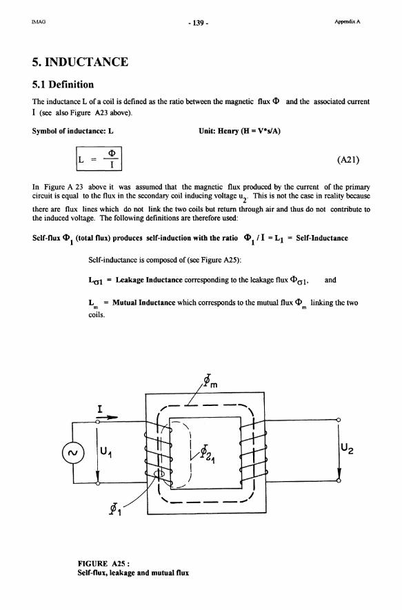
The inductance L of a coil is defined as the ratio between the rnagnetic flux cD and the associated current

I (see also Figure A23 above).

Symbol of induetanee: L Unit: Henry (H = V*slA)

(A2I)

In Figure A 23 above it was assumed that the rnagnetic flux produced by the current of the primary circuit is equal to the flux in the secondary coil inducing voltage u2. This is not the case in reality because

there are flux lines which do not link the two coils but return through air and thus do not contribute to the induced voltage. Tbe following definitions are therefore used:

Sclf-flux cD I (total flux) produees self-induetion witb tbe ratio cD I' I = LI = Self-Induetanee

Sclf-inductance is composed of (see Figure A25):

Lai = Leakage Induetanee corresponding to the leakage flux cDal, and

L m = Mutual Induetanee which corresponds to the mutual flux cD m linking the two

coils.

/- --\

FIGURE A2S: Self-flux, leakage and mutual flux


A coil has a resistance R and an induction L. These two elements can be assumed in series. The relationship between total voltage across a coil and current flowing through the coil is as follows (see also Figure A 21 above):

Utot = R i + L dI Idt , using the definition ofL we can write:

Utot = R i + N d+/dt = R i - ui where ui is the induced voltage

This formula describes mathematically what was found by experiment above: A coil having the inductance L tends to oppose a variation of current flowing through it which is, as we know, caused by self-induction. When switching on a DC voltage source (UO> on a circuit comprising a resistance R and an inductance L

connected in series, the current grows according to an exponentiallaw and reaches the end value I = uo /

R. The time constant 't is defined as:

't = L I R (s) compare with time constant for capacitors

t ..

t • UR I -1-- -~;;;..-__

U t

FlGURE A26: Development of voitage and current ac ross an inductance

Voltage ~ across the inductance has the initial value U 0 which is, according to the above formula,

equal to the self-induced voltage ui (because current i is stili zero and therefore thc ohmic part R • i as

weil). Voltage across the resistance is initially zero because source voltage and self-induced voltage of the inductance equal each other out. Final voltage across the resistor is U o' For DC current it is then similar

to a circuit with the resistor R only because L is zero due to no current variation (DC).

IMAG - 141 - AppendixA

The inductance L stores a magnetic energy of:

(Joule J) (A22)

This energy is stored in the magnetic field of the coil. It is released in form of electric current after opening the electric circuit. (Compare with the electrostatic energy stored in the electric field of a capacitor. )

5.2 Connection of Inductances

5.2.1 Inductors in series

Connecting inductors in series leads to the same formula as with resistances. Current I is constant through all inductors since the circuit offers only one path for the current to flow.

IEquivaient Inductor L = LI + L2 + L3 + ... + Lnl for series connection

(A23)

5.2.2 Inductors in parallel

As with resistances, the voltage across inductances connected in parallel is the same. This leads to the equivalent inductor for aseries of inductors connected in parallel:

Equivalent inductor L for parallel

connection (A24)

IMAG - 142- AppendixA

6. DC GENERATORS AND MOTORS

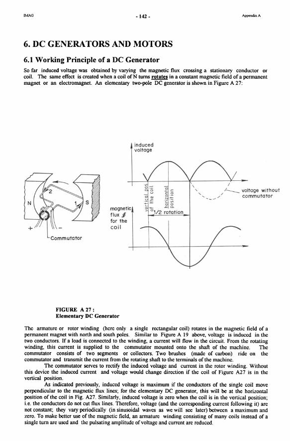
6.1 Working Principle of a DC Generator So far induced voltage was obtained by varying the magnetic flux crossing a stationary conductor or coil. The same effect is created when a coil of N turns rotates in a constant magnetic field of a permanent magnet or an electromagnet. An e1ementary two-pole DC generator is shown in Figure A 27:

Commutotor

FlGURE A27:

mognetic f lux .§ for the cail

Elementary DC Generator

induced voltage

;!c co 0 ' -

-~ :: ~'" 00 _ .c c.

> 0112 rotation

, "

I / __ voltage without

/' commutotor

The armature or rotor winding (here only a single rectangular coil) rotates in the magnetic field of a permanent magnet with north and south poles. Similar to Figure A 19 above, voltage is induced in the two conductors. If a load is connected to the winding, a current will flow in the circuit. From the rotating winding, this current is supplied to the commutator mounted onto the shaft of the machine. The commutator consists of two segments or collectors. Two brushes (made of carbon) ride on the commutator and transmit the current from the rotating shaft to the terminals ofthe machine.

The commutator serves to rectifY the induced voltage and current in the rotor winding. Without tbis device the induced current and voltage would change direction if the coil of Figure A27 is in the vertica1 position.

As indicated previously, induced voltage is maximum if the conductors of the single coil move perpendicular to the magnetic flux lines; for the elementary DC generator, this will be at the horizontal position ofthe coil in Fig. A27. Similarly, induced voltage is zero when the coil is in the vertical position; i.e. the conductors do not cut flux Iines. Therefore, voltage (and the corresponding current following it) are not constant; they vary periodica1ly (in sinusoidal waves as we will see later) between a maximum and zero. To make better use of the magnetic field, an armature winding consisting of many coils instead of a single turn are used and the pulsating amplitude of voltage and current are reduced.


The use of pennanent magnets to create the magnetic field across the rotor, known as excitation, is only possible for small generators. More common is the use of an electromagnet consisting of several field or stator coils on an iron core known as field poles. The stator winding can either be supplied by an external DC source (generator or a battery) or, as is usually the case, by the generator itself which is then ca11ed a self-excited generator. To start the induction process, self-excited OC generators can make use of the residual magnetism available in the stator poles as explained in section 3.4 above.

6.2 Working Principle of a DC Motor A OC motor is basica11y a OC generator operated in reverse. The rotor windings are supplied by euerent through the brushes riding on the commutator. While flowing through the rotor windings, the current produces a magnetic field which interferes with the magnetic field ofthe stator. Referring to section 3.5 above, we know that the resulting field creates a force couple on the rotor which provides the torque for the rotation (see Figure A 28). Note that either the stator field or the euere nt supplied to the rotor must change direction in order that the motor can rotate a complete turn.

15

_ 1_-

FIGURE A2S:

resulting mognetlc

. .!iela... . _

Elementary DC Motor

15

._ 1_ .

.-----<l+

commutotor

Nowadays the OC motor is only utilized for applications with the following demands:

- battery-driven devices (movie cameras, toys, machine tools) - adjustable motor speed over a wide range


7. ALTERNATING CURRENT (AC)

7.1 Advantages of Alternating Current Altemating current is used in most industrial or household distribution systems for the following reasons:

- lower costs for high voltage transmission as compared to direct current;

- transformation of altemating voltage and current from one level to another is easy (transformer)

- AC motors and generators are of simpler construction than DC ones (no commutator); moreover, they are more economic and require less maintenance effort;

- cutting off AC is easier than cutting offDC (when disconnecting wires (switch), sparkover is automatically stopped in AC due to the altemating waveform (zero passage).

7.2 Characteristics of the AC signal

A signal is altemating when it varies in function of time around a mean value. Its direction changes continuously from positive to negative. In electrical energy distribution systems:

- the variation is SINUSOIDAL and the mean value is zero; - the variation is periodie, i.e. it is repeated within equal time periods.

The previous section showed that all generators basically produce altemating current in sinusoidal waveform. Figure A29 below gives the explanation. According to section 4.1, voltage is induced in a conductor moving perpendicular to a magnetic field. The induced voltage is proportional to speed and length of the conductor and the strength of the magnetic field B.

u=B*I*vJ.

where v 1. is the speed of the conductor perpendicular to the flux lines.

However, the rotor winding of the generator in Figure A 29 moves only in its vertical position exactly perpendicular to the flux lines. In all other positions the horizontal velocity (the component contributing to the induced current) is lower and reaches zero when the coil is in the horizontal position. The velocity vector diagram shows the relationship between rotational speed and horizontal velocity of the coil which is obviously a sinusoidal relationship. The above formula therefore writes:

lu = B 1 v sin 0.1 (A25)

where u = instantaneous voltage v = peripheral velocity of the rotor coil

!MAG

U ,nduct'd voltogt'

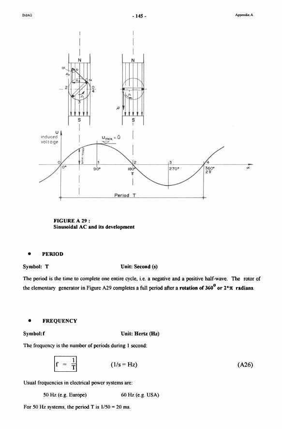
FIGUREA29 :

90·

-145 -

N

V

~~

S I

Umo~ = 0

Period T

Sinusoidal AC and its development

• PERIOD

Symbol: T Unit: Second (s)

3

270·

4

360-21T

AppcndixA

Tbe period is the time to complete one entire cyde, Le. a negative and a positive half-wave. Tbe rotor of

the elementary generator in Figure A29 completes a full period after a rotation of 3600 or 2"X radians.

• FREQUENCY

Symbol:f Unit: Hertz (Hz)

Tbe frequency is the number of periods during 1 second:

Ir = +1 (115 = Hz) (A26)

Usual frequcncies in electrical power systems are:

50 Hz (e.g. Europe) 60 Hz (e.g. USA)

For 50 Hz systems, the period T is 1150 = 20 ms.

!MAG - 146- AppendixA

• ANGULARVELOCITY ORPULSATION

Symbol: Ci) Unit: Radian per second (radis)

The angular velocity or pulsation is the angle in radian covered in 1 second. 1t is therefore proportional to the frequency f.

100 (rad / s) (A27)

7.3 Phasor Diagrams Sinusoidal wavefonns can be represented by phasors or vectors which might be added or subtracted like vectors of velocity diagrams. Figure A30 shows two sinusoidal waves, current i and voltage u, at

frequency fand out of phase by an angle <l>. Current and voltage can be represented in the phasor

diagram as two vectors rotating at an angular velocity of 00 = 2· 1t • fand with a phase angle of <l> =

a-ß· a and ß are the initial angles at t = O.

t

FIGURE A30: Pbasor diagram

!MAG - 147 - AppendixA

7.4 Notations and Definitions Instantaneous values are representcd by lower case letters (u, i) and are the CUTTent and voltage values at a specified time t.

• Peak values are the maximum values of voltage or CUTTent reachcd during aperiod T and are indicated by 0 and i.

The following relationship applies:

u = 0 • sin (00 t + ß ) i = I • sin (00 t + a. ) ifß = 0, a. = cjI

• Mean values

=> U = O· sin (00 t) and i = I· sin (00 t + cjI)

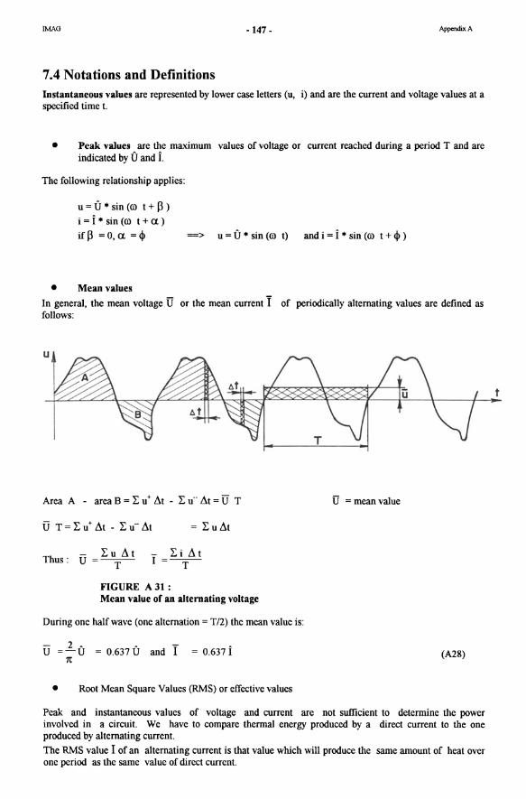
In general, the mean voltage U or the mean current I of periodically alternating values are defined as follows:

u

Area A - area B = L u + ~t - L u·· ~t = U T

Thus: LU ~t

U=-T-

= Lu~t

- Li At 1=-

T

FIGURE A3l: Mean value of an a1ternating voltage

During one halfwave (one alternation = TI2) the mean value is:

U = 1.0 = 0.6370 and I = 0.637 I 1t

• Root Mean Square Values (RMS) or effcetive values

TI = mean value

(A2S)

Peak and instantaneous values of voltage and CUTTe nt are not sufficient to detennine the power involved in a circuit. We have to compare thermal energy produced by a dircet current to the one produced by alternating CUTTent.

The RMS value I of an alternating CUITent is that value which will produce the same amount of heat over one period as the same value of direct CUTTent.

t


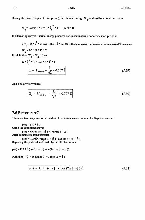
During the time T (equal to one period), the thennal energy W produced by a direct eurrent is: e

W = Power P '" T = R '" I 2 '" T (W"'s = 1) e e

In alternating current, thennal energy produced varies continuously; for a very short period dt:

dW = R '" i2 '" dt and with i = j '" sin (ro t) the total energy produeed over one period T beeomes: a

W =1I2"'R*j2*T a

Per definition W = W . Thus: e a

R*I 2 *T=1I2*R"'j2"'T e

I A

Ie = I cffcctivc = ~ = 0.707 I

And similarly for voltage:

ü I U = -r;;2 = 0.707U cffcctivc -V ,L .

7.5 Power in AC The instantaneous power is the produet ofthe instantaneous values ofvoltage and current:

p (t) = u(t) • i(t) Using the definitions above:

p (t) = Ü"'sin(ro t + ß ) * j"'sin(ro t + Q ) After goniometrie transformation:

p (t) = 1I2*Ü*j*{eos(Q + ß) - eos(2ro t + Q + ß )} Replacing the peak values Ü and j by the effective values:

p(t)=U*I*{eos(Q +ß)-eos(2rot+Q +ß)}

PuttingQ -ß =~ andifß =OthenQ =~:

Ip(t) = U I {cosp - cos(2rot+p)}1

(A29)

(A30)

(A31)

!MAG ·149· AppendixA

U(t)

wt

""t

p(t)

Ulcos1 wt

TI

FIGURE A 32 : Voltage, current and power variations versus time

Plotting instantaneous power versus time as in Figure A 32, we can observe two main features of AC systems:

. instantaneous power in AC pulsates at double the frequency ofthe grid voltage (this explains why lamps pulsate at 100 Hz in a 50 Hz grid; however, the eye cannot distinguish this frequency from any other down to about 18 Hz);

• instantaneous power comprises two terms (from equation above):

a constant power P = U*I*cos a

a variable power Pb = • U*I*cos(2ro t + )

Three distinct values of<l> are further examined:

and

a) currenl and voltage are in phase (; = 0); thus P becomes P a

because the mean value of the second term is zero. This occurs for a circuit connecting pure resistors and we can write:

P=U* I which is the same as in DC circuits (note U and I are RMS or effcctive values ofthe altemating current and voltage).


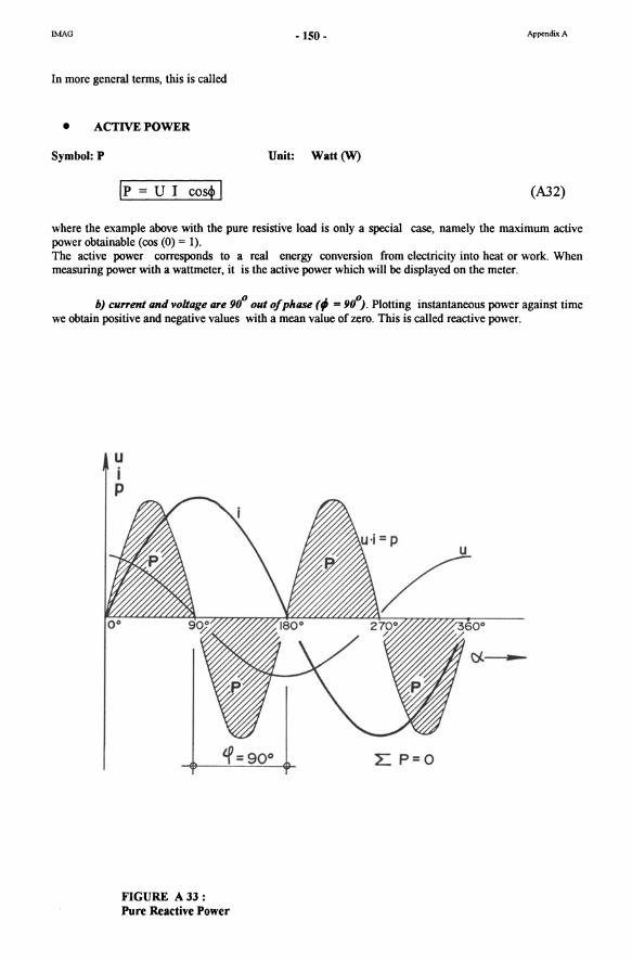
In more general terms, this is called

• ACTIVE POWER

Symbol: P Unit: Watt (W)

!p = U I coS<\>! (A32)

where the example above with the pure resistive load is onIy a special case, namely the maximum active power obtainable (cos (0) = 1). The active power corresponds to a real energy conversion from electricity into heat or work. When measuring power with a wattmeter, it is the active power which will be displayed on the meter.

b) current und voltage ure 90° out 0/ phase (; = 90°). Plotting instantaneous power against time we obtain positive and negative values with a mean value of zero. This is called reactive power.

u i p

FIGURE A33: Pure Reactive Power

L P=O


• REACTIVE POWER

Symbol:Q Unit: Reactive volt-ampere (V Ar)

Definition:

IQ U I sin<!> 1 (A33)

where our example with <p = 900 corresponds to the special case of maximum reactive power (sin 900

= 1). For<p = 9Qo no active power occurs. Power only oscillates in the circuit and is used to build up magnetic and electric fields in inductances and capacitors.

Referring to Figure A33, we can see that between t = 0 and 1t /2 a magnetic field (in a coil for example) builds up, the coil consumes energy from the source while during the next half-wave the magnetic field disappears, the coil delivers energy back to the source. Thus, no useful energy occurs.

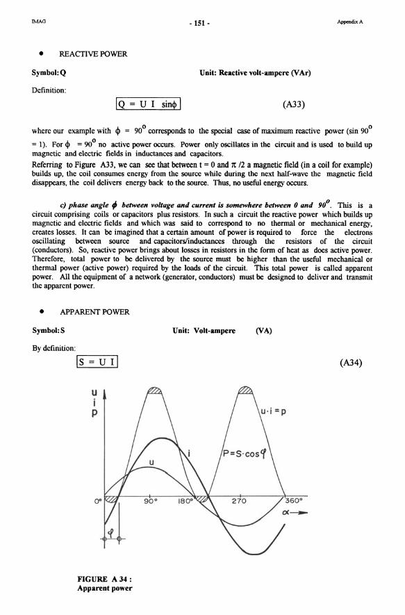
c) phase angle ; between voltage and current is somewhere between 0 and 90°. This is a circuit comprising coils or capacitors plus resistors. In such a circuit the reactive power which builds up magnetic and electric fields and which was said to correspond to no thermal or mechanical energy, creates losses. It can be imagined that a certain amount of power is required to force the electrons oscillating between source and capacitorslinductances through the resistors of the circuit (conductors). So, reactive power brings about losses in resistors in the form of heat as does active power. Therefore, total power to be delivercd by the source must be higher than the useful mechanical or thermal power (active power) required by the loads of the circuit. This total power is called apparent power. All the equipment of a network (generator, conductors) must be designed to deliver and transmit the apparent power.

• APPARENT POWER

Symbol:S

By definition:

Is

u i P

FIGURE A34: Apparent power

Unit: Volt-ampere (VA)

(A34)


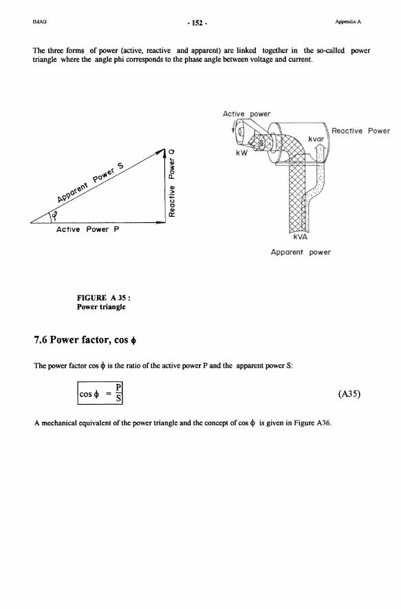
The three forms of power (active, reactive and apparent) are linked together in the so-ca1led power triangle where the angle phi corresponds to the phase angle between voltage and current.

Active Power P

FIGURE Al5: Power triangle

7.6 Power factor, cos •

o

Q)

> .0= o o Q)

a::

Active power

kVA

Apporent power

The power factor cos cl> is the ratio of the active power P and the apparent power S:

A mechanicaJ equivalent of the power triangle and the concept of cos cl> is given in Figure A36.

Reoctive Power

(A35)

!MAG -153 -

Active power P

foot pa th

rails

FIGUREA36 :

Mecbanical equivalent or tbe power triangle and cos +

o LU ~ o a.

'" > :;:::: o o ~

AppendixA

Fa

The force contributing to the displacement of the railway carriage is F . With an increasing angle p

tension in the rope increases but without contributing to the traction of the carriage. The force acting perpendicular to the railway lines is expended in pressing the wheels against the rails causing only increased friction losses. A similar situation occurs in electrical systems. The larger the phase angle between CUTTent and voltage, the stronger the electrical equipment required to generate and transmit the same active power. The power factor cos phi characterizes tbe nature of an electrical circuit. A low power factor (high phase angle) is created by inductances (creating the magnetic field in a motor for example) connected to the system. Electricity boards try to improve the power factor by insta1ling capacitors into the system (see section 8).

!MAG -154 -

7.7 Circuit Elements in AC 7.7.1 Pure Resistive Circuit

Consider a resistance R in an AC circuit with RMS values of voltage U and current 1 .

u,i,p

FIGUREA37 :

20 t ms

Phasor diagram

Pure resistive AC circuit and instantaneous values of u, i and p

Voltage U and current 1 are in phase (4) = 0, COS 4> = 1)

Ohm's law applies in the same wayas in OC circuits:

IU=R I1 according to the definitions given above:

P = U*I*cos4> = U*I = S and Q = S * sin 4> = 0

Thus:

fl

AppcndixA

(A36)

(A37)


7.7.2 Pure Inductive Circuit

Voltage of an RMS-value U is applied across a pure inductance L as shown in Figure A38.

i,u,p

FIGUREA38 : AC circuit with a pure inductance

uba,: Q=90°

I

ms

diagram

CUTTent lags voltage by a phase angle of +900 or +7tf2 radians, Le. voltage reaches its peak before the current. This is due to the opposing effect of self-induction in a coil which prevents the current to flow in phase with the voltage. CUTTent is thus limited by the so-called

Inductive Reactance XL' It represents the resistance of an inductor in AC. Reactance has

therefore the same unit as resistance, namely n . The inductive reactance is the product of the angular

velocity 0) and the inductance L (see section 5.1 above).

IXL = 0) L = 2 1t f LI where f= frequency ofvoltage and CUTTent

Similar to Ohrn's law:

Iu = XL I = 0) L I I iff= 0 (0) = 0) which is DC: U becomes zero which is a short circuit.

if f = infinite then I = 0, Le. the circuit is opened

(A38)

(A39)

As discussed earlier, instantaneous power fluctuates around the mean value zero. During a quarter of a period the power is positive and energy is stored in the rnagnetic field of the inductor and during the

next quarter this energy is returned to the source. The active power is thus zero (4) = 900 then cos 4> = 0

and sin 4> = 1):

UI cosp = 0\ (A40) On the other hand reactive power is:

Q = U • I • sin+ = U • land according to the definition above:


UXL21 CO L P = . (VAr) (A41)

Inductances consume reactive power

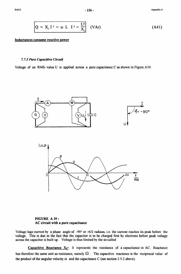
7. 7.3 Pure Capacitive Circuit

Voltage of an RMS- value U is applied across a pure capacitance C as shown in Figure A39.

i,u,p

FIGURE A39: AC circuit witb a pure capacitance

c

t ms

Voltage lags current by a phase angle of _90° or -re/2 radians, i.e. the current rcaches its peak before the voltage. This is due to the fact that the capacitor is to be charged first by electrons before peak voltage across the capacitor is built up. Voltage is thus limited by the so-called

Capacitive Reactance XC. It represents the resistance of a capacitance in AC. Rcactance

has therefore the same unit as resistance, namely n. The capacitive rcactance is the reciprocal value of

the product ofthe angularvelocity CO and the capacitance C (see section 2.5.2 above).

!MAG -157 -

Similar to Ohm's law:

COI cl

iff= 0 (CO = 0) whieh is DC: I becomes zero, i.e. the capacitor blocks a direct current. iff= infinite then U = 0, whieh is a short circuit

AppendixA

(A42)

(A43)

As discussed earlier, instantaneous power fluctuates around the mean value zero. During a quarter of a period the power is positive and energy is stored in the electrostatic field of the capacitor and during the

next quarter this energy is retumed to the souree. Tbe active power is thus zero ( = _900 then cos =

o and sin = -1):

P=U*I*cos+ =0 On the other hand, reactive power is:

Q = U * I * sin + = U * I and aeeording to the definition above:

IQ = Xc I =!c = ~I (VAr) (A44)

Capacitance generates reactive power

7.8 Impedance Z in Series Connections

Consider a resistance and an inductance in series in an AC circuit (see Figure A40). In the resistance, voltage and eurrent are in phase while in the inductanee, voltage leads eurrent by 90°. However, the same altemating eurrent flows through both elements, which creates a voltage drop in both. In AC one has to eonsider that the two voltage drops are not in phase. A resulting voltage sine-wave has to be eonstructed using vector addition. The most convenient way to do so is the phasor diagram presented in section 7.3; as magnitudes of the phasors, the RMS values are used rather than instantaneous values ofvoltage (and eurrent).

FIGURE A40: AC circuit with a resistance and an inductance in series and phasor diagram of voltage

IMAG ·158· AppendixA

The individual voltage drops ofthe elements are:

UR=R*I and UL=xLI the resulting voltage is

(A45)

the square root is called Impedance Z

(A46)

(compare with Ohm's law R = VII)

Similarly, if a capacitance is added in the circuit of Figure A40 the resulting voltage is composed of three individual voltage drops with the additional

u c = Xc * I which lags the current by 900 (which is 1800 from UL).

Thus, the general formula of impedance in series connection becomes:

(impedance for series connection of resistance, inductance and capacitance in AC)

The phase angle between the current I and the resulting voltage U is:

7.9 Impedance Z in Parallel Connections

(A47)

(A48)

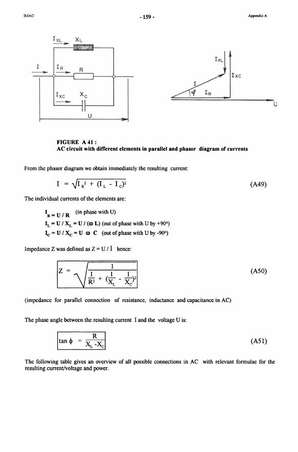
Consider an AC circuit with a resistance, an inductance and a capacitance in parallel (see Figure A41). From DC circuits we know that the voltage across each element is the same as the source voltage U. The current through the resistor is obviously in phase with the source voltage whereas the currents of the inductance and the capacitance lag or lead it by 900 or .900 respectively. To compute the resulting current, a phasor diagram of the current vectors can be constructed (again using the RMS values of the individual currents).

IMAG -159 -

-I IR R - Ixc

I xC Xc --- 11 jl

U

FIGURE A41: AC circuit with different elements in parallel and phasor diagram of currents

From the phasor diagram we obtain immediately the resulting current:

The individual currents of the elements are:

IR = U I R (in phase with U)

IL = U I XL = U I (CI) L) (out ofphase with U by +90°)

Ic = U I Xc = U CI) C (out of phase with U by _90°)

Impedance Z was defined as Z = U I I hence:

z 1 R2 +

1 1 (XL - xl

(impedance for parallel connection of resistance, inductance and capacitance in AC)

The phase angle between the resuIting current I and the voltage U is:

AppendixA

- u

(A49)

(ASO)

(AS1)

The following table gives an overview of all possible connections in AC with relevant fonnulae for the resuIting currentlvoltage and power.


TABLEA42: Overview of connections of elements in AC and relevant formulae

Connection Phasor diagram cos. Power 1. Pure Elements: a) resistance R UZ

I f=O° I coslP = 1 P=R12="R

-- - -

[3 U S = P

Q=O

U = RI b) inductance L P - 0

I eu --- S = u I

ß I cOSIP = 0 f= 900

U2 - Q=X 12=-

UL = XL I = CO L I L XL

c) capacitance C I p=o

I ~ s=uI ~

coslP =0

G UZ UZ Q=XcP=-=-

I Xc CO C

Uc =Xc I -coC

2.Series Connection P = R J2 = UZ/R -- ----UL

~ S=UZ/z=zF

ulO L!:': L1c X -Xc Q=(XL -Xc)p l..\. JUR I tanlP =~

u= z I where ~

Uc Z = impedance

Z = --JR2 + (XL - Xc)2

3.Parallel P =RP =UZ/R Connection 1L2 S =UZ/Z =z 12

1 U UZ UlaB IR R

Q=XL -Xc

Ic tan~ =--XL -Xc

I =U/Z

I 1 z~ 1/R2+ (lIXL -1/Xc)2


7.10 Resonance 7.10.1 Resonance tor series connection 0/ Land C

Consider a circuit with a resistance R, an inductance L and a capacitance C connected in series. Current is detennined by

I u z

u (A52)

and reaches a maximum value when the impedance is minimum. This happens ü XL = Xc and is

known as resonance. Since reactance is zero, current depends only on the resistor; thus Z = R and I = UIR. The phase angle between current and voltage is eliminated.

z

R-+--------""'-r--

-r--------~--------------------f

fo

FIGURE A43: Varying impedance as a function offrequency and resonance frequency for series connection

In practice, it is important to know at what frequency resonance for a given circuit occurs. The condition is XL = Xc and we obtain:

1 2 coL =-- =>CO LC=l

o CO C 0

o

(A53)

Resonance in series connections can become dangerous because the voltage across the inductance and capacitance reaches very high values. Due to their opposite position (see phasor diagrarn) these voltage values equal each other out and do not have any effect on the circuit but the coil and the capacitor themselves could be darnaged.

7.10.1 Resonance tor parallel connection 0/ Land C

In the same way as for series connection, resonance ean occur also for parallel connection of inductances and capacitors. In this case it is a resonance of currents, Le. the currents flowing through the inductor and the conductor equal each other out at a certain frequency, the resonance frequency which takes the same fonn as with series connection (see Fonnula A53). But contrary to that case, the current of the circuit takes a minimum value at the resonance frequency (Z = R).

IMAG - 162 -

Z

R-+-----~-

capacitive

-r--------~------------------~--~f

fo

FIGURE A44: Varying impedance as a function of frequency and resonance frequency for parallel connection

7.11 Correction of the Power Factor cos phi 7.11.1 General

AppendixA

The previous sections have shown how the phase angle and thus reactive power for a certain configuration of inductances and capacitors can be reduced or eliminated. The same principle is used to improve the power factor of devices requiring reactive power. The importance of a sm a11 phase angle between voltage and current (i.e. power factor cos eil elose to unity) can be summarized as folIows: for any power factor deviating from unity, power and therefore current to be generated and distributed by the electricity board is higher than the active power and current which can be converted into useful work in customers' appliances. Less power to be distributed for the same useful work means smaller conductors and generators and thus less costly installations.

In an inductive circuit, power factors are improved by connecting capacitors which power at the device, thus reducing the reactive power demand from the grid. connected:

- in parallel with motors; - in series with fluorescent tubes.

generate reactive Capacitors are

Note that the inductance of a device remains the same; i.e. its cos eil does not change but the power factor of the whole installation is improved. Reactive power oscillates between capacitor and device and, therefore, does not put load on the grid.

!MAG

I

+0-e: cu L. L. :;, U

-163 -

Capacitive

0.6 0.7 0.8 0.9 1 0.9 0.8 0.7 0.6

FIGURE A45: Variation of grid current as a function of cos eil

If cos eil = 1, then grid current I reaches a minimum value

7.11.2 Calculation ofthe Compensating Capacitance

AppendixA

cos cf

Consider a single-phase network having arated voltage U and supplying a motor. The power factor

should be corrected from cos 4> 1 to cos <1>2 by capacitors while the active power P remains the same.

IVU

•

U

FIGURE A46: Power factor correction of a motor

Active power P = U * 11 * cos 1 = U * 12 * cos 2 where

11 = grid current berore compensation

12 = grid current after compensation

!MAG -164 -

• Reactive power Q:

- before compensation Q 1 = P • tan q, 1

- after compensation Q2 = P • tan q, 2

The reactive power to be generated by the capacitance is:

Q =Q -Q =Ti'/X =Ti'roC=Ti'2XfC C 1 2 c

Ql -Q2 P (tanq,l - tanq,:J C = U2 2x f = U2 2x f (Farad)

The new apparent power to be supplied by the network reduces to:

The new current to be supplied by the grid reduces to:

(A)

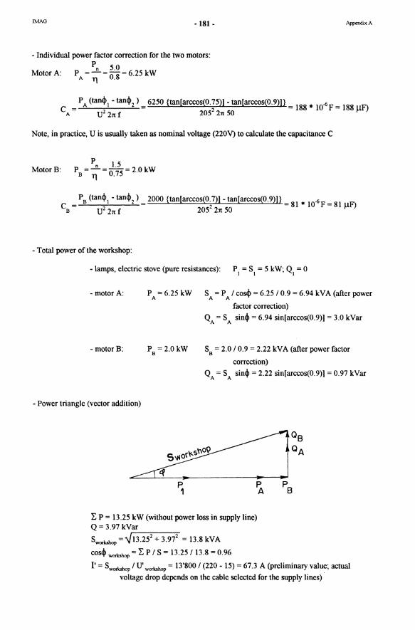
Example4: A workshop has the following electrical devices:

- Lamps, electric stove: (pure resistive loads) Total 5 KW

- Electric motor A: rated output 5 kW, efficiency 0.8, cos q, = 0.75

- Electric motor B: rated output 1.5 kW, efficiency 0.75, cos q, = 0.7

The workshop is to be connected to the local grid: single phase, rated voltage 220 V, 50 Hz. Power factor required min. 0.9 for each motor

AppcndixA

(see Table A 42 above)

(A54)

Calculate the capacitors required for the two motors (parallel connection). Determine also the cross sectional area of the supply Iines if the distance to the grid is 500 m and the voltage drop should not

exceed 15 V (using copper wire, mean temperature 20° C).

What is the total power demand (active and apparent) of the workshop assuming simultaneous operation of all loads? What will be the power factor for this case?


8. THREE-PHASE SYSTEM

8.1 General

In Chapter 7, the AC system has been introduced on the basis of a single-phase network. In practice, the single-phase system is only used for small networks « 5 kW). Transmission of bulk power over long distances is more economical using the three-phase system.

Symbol: 3_

Conveying the same power using a three-phase system instead of a single-phase one requires less than a third of conductor material (cross sectional area) despite the fact that a greater number of conductors (4 instead of 2) are used. Additionally, three-phase systems provide two different voltage levels depending on how the end-use appliances are connected to the grid (see below). The disadvantage of the three-phase system is its complexity (switchgear, monitoring, control and protection equipment for three phases rather than for one only) and the need to balance the loads over the three phases.

8.2 Generating Three-Phase Volta ge and Current

Three-phase generators may be described as 3 single-phase machines rotating on the same shaft whereby the coils receiving induced voltage are all displaced to each other by 120°. Figure A47 below shows a schematic diagram of a two-pole AC generator for a) a single phase system and the generated voltage while b) provides the corresponding three-phase system. The phasor diagram drawn from the rms voltage values of each phase shows the phase angles of 120° between the three induced voltages (or currents).

0) 9 - 0

u IVJ

prim ~ / mover,' '--___ --'

"

b) !U,

Phase t

U.

8 ' 0 -'---+- t- --r ~ /w2 v~

/Phase 3 Pha;.2'v W, '

FIGURE A 47: Two-pole AC generator for a) single phase network and b) three phase systems and the generated voltage


Note that the construction ofthe AC generator is fundamentally different from the DC generators or motors as described above although AC voltage and current may be obtained from a DC machine simply by replacing the commutator by slip rings. In practice, this is never done; AC machines employ a rotating magnetic field to induce voltage in stationary coils. Thus, the role of the stationary and rotating member is interchanged as compared to the DC machine (more details on the design of AC machines see main text).

Examining the waveforms of the three voltages produced or the phasor diagrarn, we arrive at the following concIusion:

The sum of the three voltages or currents at uy instant (t) is zero (valid for balanced, i.e symmetrically loaded three-phase systems)_

Figurc A48 shows this graphically on the basis of the phasor diagrarn.

'20 ' '20'

t,

Phosor diogram tor t,

FIGURE A 48: The sum of the voltage values in the three-phase system

8.3 Connections Instead of using 6 conductors (input and output of each coil) to transmit electricity in a three-phase system from the generator to the end-users, two or three conductors can be omitted. The three coils of the stator are

interconnected either in star (or wye (Y» or in delta (~) to produce a three phase voltage source as will be illustrated below.

8.3.1 Defmitions

Phase Voltage This is the voltage between the terminals of a coil or between any coil terminal and the neutral .

Line Voltage This is the voltage appearing between any oftwo conductors.

Phase current This is the current flowing through the stator windingslcoils of the generator (or motor).


Line current This is the current flowing through the conductors bctwccn the power station and the end-users.

8.3.2 Star or Wye Connection

Symbol: Y

One end of all three stator coils are interconncctcd to form the letter wye. The central point is callcd the neutral and may bc brought out to end-users and might bc uscd for carthing.

Une ~-------------------------------r--~~ L1 I R)

12 - I L2 UL12 UL31 <r-----....::...--==-------l--+~ L 2 (5)

V1 IV)

2

V21Yl

U1 IU) W1IW)

~------------------~N

Une Voltage ULl2

I L1 Llne LI IR)

I L L2 (5) z

::; Iu ::) L3I T)

Neutral N

r---- U1 V1 W1

~ ~ !1 (Ij ro 0::) ~

~ I1 : 1 .,

2 .,

3 In In

::> '" <> <> <> ::> .c .c s:

'l ~ 0. 1 Q.

T 0. 1 <> ::>

.c::) 0. <-U2 V2 W2

FIGURE A 49: Three-phase volta ge souree Y eonneeted lold designations in brackets)

!MAG -168 -

From such a system, the following voltages and currents are available:

IPhase Voltage Uphl = ULI N = UU! U21

I Phase Voltage Uph2 = UL2N = UVI v21

IPhase Voltage Uph3 = UL3N = UWI w21

AppendixA

(ASS)

Line Voltages Uline = ULI L2 = UU!Vl , U L2L3 = U VlWI , U L3L1 = UWIUI

(AS6)

The magnitude of the line voltgage may be obtained graphically or analytically from the phasor diagram by

subtracting the first phase voltage from the second (from Figure 50, schematic layout on the left: L U = 0 within one mesh: l!u u = .!LLl N - .!Lu N)

~ 't.;, ''-.(~~

'- '-, LI

ULiN

\

FIGURE A 50: Development of the line volta ge in Y-connection

We find:

(AS8)

This is one of the advantages of the Y - connection: two different voltage levels may be obtained from the same distribution network.

In Y - connection, the phase current I ph is equal to the line current I linie

I I line = I phase , I LI = I J I for Y - connection (AS9)

!MAG -169 - Appendix A

8.3.3 Delta Connection

Symbol: A

This is another possibility to save on conductors: In delta connection, the output terminals of each coil are connected to the input terminals ofthe following coil.

I L1 r-----------,;;..;...--------<> L 1 (R )

1L2 ,...---------='-"-----<> L 2 (S)

.--___ .... 1 .. 3>/.....--o L 3 (Tl

------~------------------L1 (R)

-----*----~~----------- L2 (S)

-----~----~----_?------------L3(T)

U2 V2 W2

FIGURE A 51 : Three-phase voltage source delta connected

Tbe line conductors are directly interconnceted via the stator windings and we find:

IUIi"< = Uu L2 = UUIU2 = Uphaoel for A connection (A60)

At each terminal of the coils (corner points of the triangle) three currents branch off: the phase current I 1

flows towards the terminal, phase current 13 flows into the coil while the difference of these two induced currents must obviously flow into the line (conductor) LI. Tbus:


This equation can be solved graphically using the phasor diagram for currents.

30'

Wl,tYV2~ __ -IIIIIII __ ~~~U2 lL~ ~ ~2

L3 L2

FIGURE A 52: Development of line currents in delta connection

Wefind:

llu =...J3 I1 or, Iline =...J3 I phase for ~ connection (A61)

8.3.4 Power in three-phase systems

Since a three-phase system is equivalent to 3 single-phase systems, we can write:

Appareot power S = 3 Uph ... I ph ...

Expressing phase current and voltage by the relationships given above for star and delta connections we find for both types of connections:

I s =...J3 Vline I linel (VA) for Y and ~ connection (A62)

Impedance

We define an impedance ofphase Z, which is the ratio between voltage and current:

Zph ... = Uph ... ' ~h'"


Y connection: (A63)

A connection: (A64)

8.3.5 Conclllsion

Y connection gives a higher terminal voltage than delta connection but a correspondingly sm aller output current.

The same relationships are valid not only for generators but also for motors and other end-use appliances. Using the same principle, a motor of a certain impedance connected in star (Y) to a given network voltage

(Uline) will draw only a third ofthe CUTTent as compared to delta connection (A). This feature is used to limit

the starting current of asynchronous motors which usually have starting currents of 4.5 to 6 times the nominal current; Le. the motor is first connected in Y up to almost nominal speed, whereby drawing a

current only slightly above nominal (1.5 to 2 times), and then switched into A connection to develop full operating power and torque.

Comparing impedances in the Y and A connection, we may conc\ude the following (see Formulae A63 and A64 above):

To arrive at the same voltage and cUTTent levels, phase impedance in A connection must be three times higher than the corresponding impedance in Y connection .

(A65)

8.4 Rotor Speed and Generated Frequency Rotor speed and frequency of the generated voltage are direct1y related. Consider the e1ementary two-pole AC generator ofFigure A47 above. Applying DC CUTTent to the field winding on the rotating rotor creates a rotating magnetic field which induces voltage in the stator coil(s). Obviously, turning the rotor one complete turn generates one cyc\e of AC voltage. Rotating the rotor one turn in one second gives one cyc\e per second or 1 hertz (Hz) as the frequency is referred to (frequency is directly proportional to the speed ofthe rotor; see also section 7.2 above). If the rotor has more than two poles, say 2p poles, each revolution of the rotor induces p cyc\es of voltage in the stator coils. Note that due to the continuous nature ofthe magnetic field lines, the magnetic poles always occur in pairs, hence, 2p can only take the values of 2, 4, 6 etc. Thus, we can write in accordance with Formula (A27) above:

Ir = p 6nol (Hz) (A66)

where f= generated frequency (1/s = Hz) n = rotor speed (rpm, revs per minute) p = nomber ofpole pairs (where p must always be an integer)

To produce voltage of a given frequency, the rotor must be turning at a speed compatible with this frequency, Le. the rotor must rotate at synchronous speed. The common frequencies of 50 and 60 Hz are obtained with the following rotor speeds and nomber ofpoles (using Formula A66 above):


TABlE A 53 : N b f I um er 0 po es an d sync ronous spee s 0 t h d f h ree-pr ase motors an generators h d

Number of poles SO Hz grid frequency 60 Hz grid frequency 2 3000 rpm 3600 rpm 4 1500 rpm 1800 rpm 6 1000 rpm l200 rpm 8 750 rpm 900 rpm 10 600 rpm 720rpm

Generally, generators with as few poles as possible are to be chosen in order to reduce size and costs of the machine. However, the speed is usually determined by the prime mover: Waterwhccls for example require a large number of poles, because of their low speed while high speed applications such as Pelton turbines under high heads may make do with 2 or 4 pole generators even if direct-coupled. On the other hand, low speed generators with many poles may not be alIected in their structural integrity when the turbine/generator unit accelerates to runaway speed. Runaway speeds of turbines are in the order of 1.5 to 2 times nominal speed. A two-pole generator may therefore accelerate up to 6000 rpm at fullioad rejection and hearings and rotating elements are likely to be damagcd at such speeds; whereas low speed generators with many poles may even rotate at runaway speed for extended periods without being damaged.

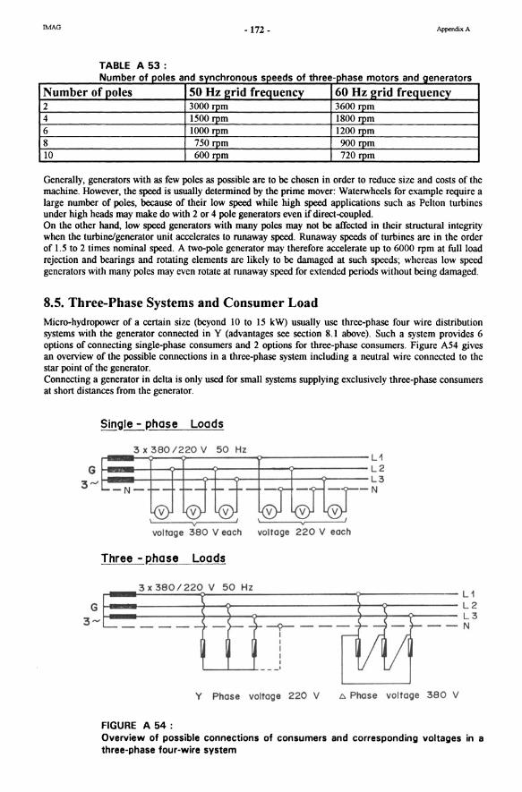
8.5. Three-Phase Systems and Consumer Load Micro-hydropower of a certain size (beyond 10 to 15 kW) usually use three-phase four wire distribution systems with the generator connected in Y (advantages see section 8.1 above). Such a system provides 6 options of connecting single-phase consumers and 2 options for three-phase consumers. Figure A54 gives an overview of the possible connections in a three-phase system incIuding a neutral wire connected to the star point of the generator. Connecting a generator in delta is only used for small systems supplying excIusively three-phase consumers at short distances from the generator.

G 3 ......

Single-~hase Loads

volfage 380 V eoe" volfage 220 V eoeh

Three - ~hase Loads

3)( 380/220 V 50 Hz

I I L _____

- ~~---~- ~- - ~--I

~vtt1 I I I I

--. Y Phase voltage 220 V t:. Phase voltage 380 V

FIGURE A 54:

Li L2 L3 N

Overview of possible connections of consumers and corresponding voltages in a three-phase four-wire system

!MAG - 173- AppcndixA

In a three-phase system, several single-phase appliances together (lighting, other srnall household appliances) constitute a three-phase consumer. It is important that these single-phase consumers are connected to the grid in such a way that all three phases are equally loaded. Tbe three-phase generator is designed to deliver a third of the total power through each phase. Imbalanced loading of phases (e.g. all lamps of a whole village on phase I) rnay create a situation where excess power flows through one or two phases, overheating the windings and finally causing the insu1ation to burn and the generator to fail. In an imbalanced system with the neutral connected to the starpoint , a fairly high current rnay flow back to the power station. Eliminating imbalances is very difficu1t for srnall grids because relatively large singlephase appliances connected to the same phase rnay be switched on simultaneously overloading the generator (that is why small grids preferably use single-phase systems). In larger grids, imbalances on phases rnay equal each other out according to the laws of probability provided that the single-phase appliances are weIl distributed over the three phases. Tbe current in the neutral indicates whether the system is weIl balanced or not:

l There is no current in the neutral wire in a balanced three-phase systeml

Tbe current in the neutral wire can be calculated by adding graphically or analytically the vectors of the three line currents ofthe system (see example 5 below).

Example5:

A three-phase four-wire system (380/220 V; 50 Hz) has the following loads:

- three-phase motor connected in Y with the following name plate data:

- resistive load (electrical stove) between LI and Neutral: 2.5 kW between L2 and Neutral: 5.5 kW

U = 380 / 220 V (Y / A) I = 30 / 52 A PN = 15 kW

cos 4> = 0.85

- capacitive load and resistive load in series between L3 and Neutral: R = 5 n and C = 318 J.1F.

Calculate the phase currents ofthe appliances, the line currents and the current in the neutral wire.

8.6 Power Factor Correction in Three-Phase Systems Basically, power factor correction in three-phase systems is similar to the procedure shown for single-phase networks; the same formulae as given in section 7.11 above apply. Tbe ouly difference is that in a three phase system the capacitors rnay be connected in Y or in delta. From formula A65, we can see that the

capacitance C6 is always smaller than Cy (for capacitor Zc = Xc = l/roC). That is why capacitors for power factor correction are usually connected in delta despite the higher voltage and thus higher insulation c1ass required. Using the following general indications, the required capacitors can immediately be determined from the reactive power to be compensated per phase (valid for a 380/ 220 V; 50 Hz network)

Compensating reactive power of 1 kvar in Y - connection (220 V/50 Hz) requires

capacitors of 66 JJ.F Compensating reactive power of 1 kvar in A - connection (380 / 50 Hz) requires

capacitors of 22 JJ.F


Example 6: A three-phase motor is connected in Y to a three-phase four-wire system (380/220 V; 50 Hz). The name plate provides the folJowing data:

u = 380 / 220 V (Y / A ) I = 30 / 52 A

PN = 15 kW

cos<ll = 0.85

The power factor should be corrected to cos <Il = 0.915. CaIculate the reactive power to be provided by the capacitoTS and the size ofthe capacitors in delta connection.


9. VOLTAGE DROP AND CONDUCTOR SIZE

9.1 General For short supply lines, the conductor size is based on keeping heating of the conductors within acceptable limits (see Table in Appendix BI). For longer lines, it is the maximum acceptable voltage drop which determines the conductor size. Some loads 1 consumers are sensitive to large voltage variations (e.g. motors) while others are less (e.g. incandescent lamps). If no details of the future appliances are available, the following maximum voItage drops may be used to determine the conductor size:

• House and factory installations: - For main lines as far as the main fuse in buildings: max 0.5 %

- For light installations: max 1.5 %

- For power installations: max 3 %

• Distribution liDes: - 10 % (ifthe admissible voltage variation ofappliances is ± 10 %)

9.2 Volta ge Drop in DC

Referring to Ohm's law U = R I and the formula for resistances R = P l1 A (see section 2.1 above), we can immediately calculate the voltage drop of a line in DC:

(A67)

Where U v = voltage drop in the conductor in V « permissible voltage drop as indicated under 9.1 above)

p = resistivity of the conductor material (0 mm2/m) I = single length of the conductor between source and end-user (m)

I = current (A) A = conductor cross sectional area (mm2)

Note that the factor 2 allows for the voltage drop on the line from the appliance back to the voltage source.

Or solving the equation for the minimum cross sectional area required to keep the voltage drop Uv below

the permissible value:

(A68)

9.3 Volta ge Drop in Single-Phase AC 9.3.1 Considering line resistance only

Note that the following formulae are only correct if the inductance of the cables and conductors is negligibly small as compared to their resistance. This applies to most low-voltage (LV) house wiring and factory installations but not necessarily to distribution Iines in micro-hydropower systems. For the latter cases, we recommend that the cables should be pre-selected using the formulae for ohmic losses but the final selection should be made only after the total voltage drop including the reactance of the cables has been checked (using Formula A71).

An additional problem arises for inductive loads: the voltage drop ofthe cable (line) is not in phase with the voltage of the consurner. Figure A55 below shows the circuit diagram oi a single-phase motor (inductive consumer) connected to an AC generator. Due to the voltage drop on the line, the motor does not receive

!MAG - 176- AppcndixA

full generator voltage. Unlike the DC case, only that part of the total voltage drop in the conductor (Uwire)

which is in phase with the consurner voltage must be considered as the effective voltage drop (U) for the motor. This is illustrated with the phasor diagram in Figure 55 below. Since Uwire is usually small as compared to the voltage drop across the consurner, we can calcuiate Uv approximately as follows (assuming

that AB ~ AC on Figure A 55):

Uv = Uwire cos<!>. Since Uwire is equal to Uv in DC (see Formuia 67 and 68) we can write:

IA=2 pI Jv

cos4J I where Uv = permissible voltage drop for the application

RmOlot

Ugil!'nttrotor

Xmoto,

~

UR

single- le-ngth

u,.". not to sco Ie-

lJgt-nrrotor

FIGURE A 55: Voltage drop in a single-phase AC system with an inductive load

9.3.1 Considering resistance and indllctance 0/ a line

lf the reactance of a cable becomes important, the following formula may be applied:

mH!km (milli-Henry / km)

where d = distance between two conductors and r = radius of a conductor

andX=L· 21tf [n /km]

(A69)

(A7I)

Refer to manufacturers brochures for the thickness of insolation materials between phases in composite cables.


For a 50 Hz grid, the reactance X of overhead Iines is about 0.4 n / km and for cables 0.07 to 0.17 n / km

The total voltage drop can be found using the two components UR. wire =2 ... R • I (in phase with I) and UX •

wire = 2'" X'" I (900 out ofphase with I) and adding them graphically (see also Figure A56 below). Note that the factor 2 allows for the voltage drop on the line from the appliance back to the voltage source.

Assuming that <\> load == <\> total = <\>, we can write:

Total voltage drop U v = 2 (I R cose!> + I X sine!» < permissible voltage drop for the application

Rw ,rll!' Xwj,r I

URwlrr UXwr1'"1!' Rmol

Xmol . Ugrne-ro\or RwlrIP X WIJ"f'

~ -URwire- UXwirot

sin t h I

FIGURE AS6: Total voltage drop in a single-phase system including resistance and reactance of

the supply line

9.4 Volta ge Drop in Three-Phase AC Three-phase systems are basically 3 single-phase systems with only one return wire. It is usual practice to assume balanced loads for the calculation of the voltage drop, Le. the neutral wire is without current. Therefore, the same formulae as for single-phase systems apply but calculated with the single length of the line:

• considering line resistance only:

IA= pI ~:o~ I (A70)

• considering line resistance and reactance

luv = R I co~ + X I sin<\> I (A7l)

Example 7: In an irrigation project, a pump with a 30 kW three-phase motor has to be connected to a three-phase

network (380/220 V , 50 Hz). The pump house is 250 m away from the switchboard. The motor has a cos<\>

ofO.87 and an efficiency TJ = 89 %. Admissible voltage drop is 3 %. What size of alu cable is to be chosen?

(P.'u = 0.03 n mm2/m at 200 C)

IMAG - 178-

10. ANSWERS TO THE EXAMPLES

10.1 Example 1/ page 120

Resistances for each appliance / device:

-Lamps:

2 Un 242

R =-=-=23n 1 P 25

n

242 R =-=576n

2 10 .

242 R =-=384n 3 15 .

122 R =R =-=9.6n

4 5 15

- Wiring: p Cu200C = 0.0175 n mm2/m

° _e....! 0.0175· 2· 200 - n Rcu20 C - A 1.5 - 4.67

° 35 - 20 Rcu35 C = Rcu20 (1 + 235 _ 20) = 5.0 n

- Circuit diagram and equivalent circuit

'2v+I ~ -1L--~RC ]---L.L.LJ

200m

~quivalent circuit

I -

~

AppendixA

!MAG - 179-

- Equivalent resistances:

series: R4 _5 = R4 + ~ = 2 * 9.6 n = 19.2 n I 1

parallel: R I_3 = IIR + IIR + IIR 1/23 + 1/57.6 + 1/38.4 11.5 n 1 2 3

parallel: R I_5 = IIR + IIR I

1/11.5 + 1/19.2 7.2 n 1-3 4-5

series: R = RI_5 + Ra. = 7.2 + 5.0 = 12.2 n

- Voltage available: U = 12 V;

- Current in the supply line:

- Power requirement:

1= UIR = 12 /12.2 = 1 A

P=U*I=12*1=12W

- Conductor size: 1. Kecping heat within acceptable limits (see Table BI, main volume)

Maximum current for a 1.5 mm2 section: 10 A > I actual = 1 A

2. Voltage drop

U = R • 1= 5.0 • 1.0 = 5 V v c => 42 % ofUsource

AppendixA

far too much > use a larger cross section (see also Chapter 9).

- Available voltage on the lamps:

U1amps = R • 1= 7.2 • 1.0 = 7.2 V 1-3 1-5

(very low as compared to their rating of 24 V -> will not light up) U1amps 4-5 = 7.2/2 = 3.6 V

(also too low for their rating of 12 V)

- Conclusion: The example shows that a 12 Volt DC source is insufficient to supply a house with a number of loads at 200 m distance. A larger conductor size may improve the situation but will most probably pose economical problems.

10.2 Example 2 / page 124

2 W 2 * 100 -4 C=-2 =--2-=3.13 *10 =313 IIF

U 800 ,..

circuit diagram:

~U=800 V

!MAG -180 -

Maximum current at the beginning of the charging process:

U Uo 1.5 io=imax = RO <O.IA => R,. > -. - = - > 150 eq l max 0.1

10.3 Example 3 I page 125

- The second capacitor is twice as big as the first one: 2 CI = C2

- For paralIel connection: Ctolal = CI + C2 = CI + 2CI = 3 CI

CI = CtoIal /3 = 104 JlF ; C2 = 2 CI = 208 ~F

- For series connection: 1

CtotaJ = Cequi = IIC + I/C I 2

IICI + 112CI 2CI 13

C2 = 2 CI = 940 ~F

The parallel connection is to be preferred.

10.4 Example 4 I page 164

I 1- -WOrkshOp- - - -1

Supply -l I ~: I

220 Vl-1 .>c: I I 50 Hz I 0 ~ I I

::::!: I I ~ __________ ~ __ ~~ __ ~~ __ L~ __ ~ I

500 m L ----1----J

AppendixA

u= 205 V

!MAG - 181 - AppcndixA

- Individual power factor correction for the two motors:

Pn 5.0 Motor A: P =-=-= 6.25 kW

A 11 0.8

PA (tan<!>1 - tan<!>2) 6250 {tan[arccos(0.75)] - tan[arccos(0.9)]} 188 * 1O-6 F = 188 /lF) CA U2 211 f 2052 211 50

Note, in practice. U is usually taken as nominal voltage (220V) to calculate the capacitance C

MotorB: Pn 1.5

P =-=-=2.0kW B 11 0.75

PB (tan<!>1 - tan<!>2) 2000 {tan[arccos(0.7») - tan[arccos(0.9)]} CB 81 * lO-6 F = 811-lF)

U2 27t f 2052 211 50

- Total power ofthe workshop:

-lamps, electric stove (pure resistances): PI = SI = 5 kW; QI = 0

- motor A:

- motorB:

- Power triangle (vector addition)

PA = 6.25 kW S A = PA / cos<j> = 6.25/ 0.9 = 6.94 kVA (after power

PB =2.0kW

factor correction)

QA = S A sin<!> = 6.94 sin[arccos(0.9») = 3.0 kVar

SB = 2.0 / 0.9 = 2.22 kVA (after power factor

correction)

QA = S A sin<!> = 2.22 sin[arccos(0.9») = 0.97 kVar

~ P = 13.25 kW (without power loss in supply line) Q = 3.97 kVar

Sworkshop = .."jri-3.-25-:;2:-"+-3-.9-772 = 13.8 kVA

cos<!> workshop = ~ P / S = 13.25/ 13.8 = 0.96

I' = Sworkshop / U' workshop = 13'800/ (220 - 15) = 67.3 A (preliminary value; actua1

voltage drop depends on the cable selected for the supply lines)

IMAG -182 -

- Conductor size required for the supply lines (see also Chapter 9)

admissible voltage drop at workshop: Uv = 15 V (in phase with workshop voltage)

==> voltage drop in supply lines: Uwire < Uv I COs4>wOrbhOP = 15 10.96 = 15.6 V

R < Uwire 1 1 = 15.6/67.3 = 0.232 n c

resistivity ofcopper: P200 C = 0.0175 nmm2 /m

Ll_ 0.0175· 2· 500 75.5 mm2 A> R - 0.232

c

From Table BI: diameter = 12.5 mm, A = 95 mm2

(Note that in this case, the criterion for the selection ofthe cable is not heating but voltage drop.)

_21_ 0.0175· 2· 500_ Ractual - A - 95 - 0.184 n

AppendixA

Total voltage drop U'wire = Ractual • I' = 0.184 • 67.3 = 12.4 V (in phase with I' but not with U'worbho~

Phasor diagram:

4> worbhop = arccos(0.96) = 16.30

U' = (U' . '" )2+(U, "'" +U' )2= gen worbhop SIn"'worbhop worbhop C0"'l'worbhop wire

U'gen = ..../(205 • sinI6.3°i + (205 • cosI6.3° + 12.4i = 217 V

Voltage available at the generator is 220 V

~ == I' • U/U' = 67.3 • 2201217 = 68.2 A

Total apparent power S = U • l total = 220 • 68.2 = 15 kVA (at generator)

Power factor at generator (all appliances connected): (from phasor diagram above)

205 • sin16.3° tan4>total = 205.0.96 + 12.4 0.275

=> <l>total = arctan(0.275) = 15.40 and cos4>total = 0.96

!MAG


L 1 3 x 380 / 220 V 50 Hz

-183 - AppendixA

1 L2--------------~~----------}_----~--------------

L3--------------~--}_~--------+_----_7------_?--------

N --- ---- ---~ +--U1 V1\ W1 , .~ I, -~---<r---+-b----<2 r--~:J

Motor, PN "'15kW ~"'2.5kW f2 5.5 kW C=318"uF R3"'5.J'l. In '" 30/52 A ,cos f=0.85

L Determine the currents for each phase as for a single-phase system

Eguivalent circuit

- Motor in Y (from name plate):

I = I = I = 30 A-m} m2 m3 '

sin!\> = + 0.527 (ind.) ; m

- Stove (cos4> = 1)

cos4>m = 0.85 (ind.)

4> = 31.790 (ind.) m

I = P/U = 2500 / 220 = 11 4 A . '" = 0 Rl ph . ,,+,

I = P/u = 5500 / 220 = 25 A . J. = 0 R2 ph ' '+'

- Resistance and capacitance in phase 3:

X = 1/ (00 C) = 1/ (2 1t f C) = 10 n c

-v 2 2 __ ~_ n from Table 40: Z = R3 + Xc - 'IJ 5 + 10 - 11.18

IR3 = IX(; = Uph 1 Z = 220 / 11.18 = 19.68 A

tan4> = X 1 R = 10 1 5 = 2.0 ; 4> = 63.430 (cap.) c 3 c cos4> = 0.447 (cap.) ; sin4> = - 0.894 (cap.) c c

N I 0 L1 '" &f '" " 0 <Xl

'" M

'" ."

i3

!MAG - 184- AppendixA

2. Resultant currents per phase (to be determined with phasor diagrarn)

- Phase I

I = A '(I cos<!> + IR / + (Im sin4> )2 = 40.1 A 1 \I ml m 11m

Im] cos4>m + IR] . cos4> ] = I = 0.920 (md.) 4>] = 23.0°

]

- Phase 2

12 = 52.9 A cos 4>2 = 0.954 (ind.) 4>2 = 17.4° (ind.)

- Phase 3:

I = (I cos4> + IRIX cos<!> i + (Im sin4> - IRIX sin4> )2 = 34.3 A 3 m3 m 3 C 3 m 3 C

A. = 300 'f'3 .


3. Current in neutral

- Phasor diagram for voltage: Uph = 220 V, each phase 1200 displaced

- Line (= phase) currents to be plotted into the voltage phasor diagram taking into account the different

phase angles <!> (leading or lagging): inductive => lagging voltage capacitive => leading voltage

• UPh1

I inductive = Jogging

I I I

Ineutral == 31 A (rclativcly high imbalance)

copocltive =

- Refer to max. admissible imbalances of generators indicated by manufacturers. 4. Total power of a11 consumers together

- active power for non-symmetrically loaded systems: P total = P phI + P ph2 + P ph3

P = U I cos'!" = 220'" 401'" 0 920 = 8109 W phI ph phI 'VI ..

P = U I cos'!" = 220'" 52.9 ... 0.954 = ph2 ph ph2 'V2

Pph3 = Uph I ph3 COS<!>3 = 220 ... 34.3 ... 1.0 = Ptotal =

11'105 W

7536W

26'750 W

- similarly for total reactive power: Qtotal = Qphl + Qph2 + Qph3

with Qph = Uph I ph sin<!> Qtotal = 7.35 kVar

- total apparent power Stotal = --.j'p-total-=-2 +-Q-to-tal""2 = 27.74 k VA

rotation



The efficiency of the motor is not known, i.e. the electrieal power must be deterrnined using voltage and eurrent indications:

P e\ = V3 Uline I line eos4> = V3 • 380 • 30 • 0.85 = 16'800 W

- Capacitors in fl : (eaeh capacitor will receive line voltage Uline = 380 V)

Li

I IU ,ine L2

I L3 r discharge reslstors

8 C - P(tan</ll - tan</l2) 16'800 {tan[areeos(0.85)] - tan[areeos(0.915)]} 22. 10""F = 22 ~F

Nphue - 3 U2 21t f 3 • 3802 21t 50


3 x 380/220j50Hz Re

N Li L2 L3

+ 250 m

lUne

! 8

IMAG -187 -

p.1 = Pn 111 = 30 10.89 = 33.71 kW

_ h Pe! 33'710 P I = V 3 Uline 11m. cos<\> => l lin• = _ h '" = _ h3 * 380 * 0.87 58.87 A

• m V3 Uline COS'!'m VJ

- admissible voltage drop Uv = 3% ofUn = 0.03 • 380 = 1l.4 V

- voltage drop in phase with currentI: Uwir< = U I cos<J> = 11.4 I 0.87 = 13.1 V v m

R.Ju < Uwirel 11m. = 13.1/58.87 = 0.223 n

A> Palu * I1 R.Ju = 0.03 * 250 I 0.223 = 33.7 mm2

- Cable selection (see Appendix BI):

criterion heating: 1 = 58,9 A => A > 16 mm2

criterion voltage drop: A > 33. 7 mm2

- Pre-selection: cable diameter: 9 mm A = 50 mm2 per phase

- Verification of total voltage drop including the reactance of the cable: from manufacturer's brochure:

Cable 3 X 50 mm2

E E O'l N !

L = 0.05 + 0.2 In(12 I 4.5) = 0.246 roH I km

x wir< = ro L = 21t 50 * 0.246 * 10-3= 0.077 n I km or for 1 = 250 m => X = 0.02 n

Rw. = Palu *11 A = 0.03 * 250150 = 0.15 n

Total voltage drop U == 1 *R * cos<\> + I * X * sin<!> = v

58.9 * 0.15 * 0.87 + 58.9 * 0.02 * sin [(arccos(0.87)) = 7.69 + 0.56 = 8.25 V < U adrn. = 11.4 V

v

AppendixA

!MAG -188 - Appendix B

APPENDIX B

SELECTED DIAGRAMS AND TABLES FOR ELECTRICAL ENGINEERING DESIGN

Appendix BI

Standard Wire and Cable Sections and Permissible Currents (Heating Limit)

Standard Wire Wire Diameter Cable Diameter Maximum Maximum Section Current Current

(mm2) (mm) (mm) Stationary Moving Installation Installation

(A) (A)

0.75 1.0 6 1 1.13 6 10

1.5 1.4 10 15 2.5 1.8 15 20 4 2.25 20 25 6 2.8 25 40 10 3.6 4 40 60 16 4.5 5.1 60 80 25 6.3 80 100 35 7.5 100 50 9 125 70 11 150 95 12.5 200


Appendix B2:

End-Use Appliances and their Approximate Power Demand

Appliances Nominal power in Watt Lighting: - Incandescent lamps 25 - 200 - Fluorescent tubes 25 - 100 - Energy-efficient lamps 8 - 25 Heating: - Boiler 100 I 2400 - Boiler 1000 I 8000 Household appliances: - Cooker / stove (single hotplate) 1000 - 2000 - Cooker I stove (3 hotplates) 6000 -7000 - Low-wattage cooker 200

- Refrigerator 180 litre 100 - Deep-freezer 300 litre 200

- Washing machine 2100 - 3300 Electronics: - Radio (portable) 10 - 100 - Radio (stationary) 100 - 300 - TV (colour) 200

- Computer 200 -250 - Printer 80 - 150 Workshop: - Circular saw 2500 - 5500 - Centre lathe 1500 - 5000 - Universal milling machine 1500 - 3000 - Bench and pillar drilling machine 500 - 1500 - Angle grinder 500 -1500

Source: - FAT, Switzerland: Rapport 348 - International Labour Office, Geneva: Equipment planning guide


Appendix B3

Efficiencies and Power Factors for Induction Motors (average values or standard motors)

l~ . ~ ~~ -"'-~: t;:

~;~ =- \:: .'\

:- ~~ .~

-! ~

VI 0 ...

-tNO<DUl Ci> Ci> Ci> <D Cl)

ci 0 Ci ci ci

-t N <D <D ci ci

o <D ci

'\ '\

I\.

""-

'" '\.. ,

.........

I

t-...

N r--ci

-"

o m Ul r-- Ul Ul ci ci ci

0 Ci Q

g on Q 0 -t 0

~ 0 Ci N

0 Q

Q on

0 rti

0 N

9

., 0

~ 6

c n.. 0> c:

-.::: 0 -0 .§ .. cu ~ 0 Q.

-~ e ~ 0

"C ... -g ...

!MAG -191-

Appendix B4

Slip versus Mechanical Power for Induction Machines (for "bard" non-saturated motors only)

~

c -

~

VI

t--- -"S VI

~ - -

I VI

I ~ -

E I I ~ -

c - .2 ..

CI ... Q)

~ Cl. 0

li2 ~~ t---I &

I I I

I I I I

I I ---'---

11 I I

-t

1+

1 I- +

o [8

o lO !fl

o 0 0 <:t N 0 !!2 !!2 !fl

1

I

I

o Q)

~

I

\

I

I i I I I

c 0 ;: CI ... Q) Cl. 0

... 0 .. 0 E e--- ---

\ \ '\

1\ 1\

o 0 N 0 ~ ~

0 10

0 <:t

0 r<l

o N

o

3 "" -n.c

~

CI C

~ ~ -... Q)

~ 0 Cl. .. :::J Cl. .. :::J 0

'0 Q) -CI ...

Appendix B


Appendix B5

General Range of Efficiencies for Synchronous Generators

E e-0 0 ~

r!'

CI) L-0 -CI L-CI) c CI)

0 co c CI)

U CI)

;;: :::l 0

't- C CI) 0

"-CI) .c

0 :::l C CI)

"- >. CI) CI)

> CI) - 0 :::l 0-0--:::l

0 V

~ - I I I I

r-- lD I() 'Jj r<l '" äi 0 m OJ CD OJ OJ CD CD CD r-- r--

u 0 0 v VI ci. E ~ -C CI)

:ci E CI

J: E

CI) 0 CI)

CI 0 u 2 C VI 0 -.: CI)

CI " :::l :::l -CI) -.: c «

r-- lD I()

r-- r-- r--

L-0 -0 CI -"-CI)

~ 0 0-

CD 0 -CI

I

<J" r<l '" r-- r-- r-- r:::

o ~

o I()

'"

Q o '"

Q I()

Q Q

~o i I()

1 r--

lMAG -193 - Appendix B

Appendix B6

General Range of Efficiencies for Couplings

Type 0/ coupling maximum max.power general advantage/ gearing per stage in range 0/ disadvantage ratio kW efficiency (single (per stage) staKe)

Flat belt + simple

-d - high initial tensioning (forces

5 > 100 96 - 98 % on shafts) - careful alignment required

V-belts

• + readily available + quiet + do not require

8 35 94-97% very precise alignment - high initial tensioning

Toothed belts + high efficiency

(timing belts) ~~ + no slip ... ~ .. ~ + litde initial ,;""'-~ -, ~ 98% tensioning

~~,~-- - noisy - expensive - not readily available

Chain drives

~ + high efficiency + no slip + no initial

6 200 97 - 98 % tensioning - expensive - maintenance

I (lubricaticn)

Gear box:

~ + require less space

Spur gears than beIts - expensive

D 8 96-98% - maintenance

~.~

Gear box: ~~

+ connect

Bevel gears intersecting shafts fc-"; :.J - expensive C::--::;y: .. M_,..~ 6 96-98% - maintenance

~~-1. • \\p

1~1 1I i \~ 11---

-----Source: - Niemann G. : Maschinenelemente, VoL 11, 1965 - Dubbel: Taschenbuch für den Maschinenbau, 1986 - various manufacturers' brochures


Appendix B7

Turbine Types and Specific Speeds (in function ofhead and flow)

(adapted from BundesamtjUr Wasserwirtschaft: Kleinwasserkraftwerke in der Schweiz, Part 1,1983)

-t Gl!T1 co ::c". cr '" 0 :r ::::J 3

[rpmJ '" "0 Turbine Rotatlonal Speed n

0 ..

01 ~ I

N~ 01'" (]I m Ö Gi 0 0 " ::1 N g äi~ 0 0 0 0 0 ::::J 11 --IN '" (]I cg.., !So UI(%) 0 0 0 0 0 (]I

··0

~ 8 3 ::::J 3: e.Q 0

~ § 0 11

'" (5 -.J -;-" ::::J<II

0 (]I_. f .....

I I o!! -0- "' ....... -..., "0 ~:E

"'0 '" OQ 3 ::; o ..., ::::J"O"

------k---L--_ c 3 0 - 1;;

lir

,0 , ~ --! 0 I~ ,

I I , ,

! I .~ .~ I Speciflc Speed

I

! -$~~

N N 01 ..... o ur 0 ur

Z CD -:z: CD c a.

:z: :::J

:E

n q .. n-.JQ,;'

H" 3/4

I s ingle jel ~mult jel

~ Petron - - - -+-- -=-- Francis -------1- Kaplan

Cross - flow @~

1.2

1.5

2

3

4

5

10

20

30

40

50

100

150

200

300

400

500

100

(tu

rbIn

e

[%]

~

Fra

ncls

I

Kap

lan

90

I

-~

:.;

;; .

. ?;;:

' :,.~

f .

,",

~ ,

'.

-':'"

:,

' \:'"

.'

' ..

. :'.;

'. ,"

::.':

.

: .~

.' :.:' ,:

: :'. ,:"

P~l

to'n

.'~·

·.: ;

', . : ~

,,' ~ : ~.

::.

~: . ,'

......

....

.....

'.'

,'"

".

~ """"

"" ~ ~"""

""'" '" '\' ~"'''

'' '" '" '" '\

~ ~~ ~ '\.

'\. '\. "\.

"\. " C

r6ss

-FIO

.... ~""~~ ~"'~ ~~~

.~ ~

" -" ,-"

" "

---

-=--

--~ t-

-1--

--;'

80

70

60

50

/ P

AT

• P

umps

us

ed

os

Tur

blne

s 4

0

I I

I -

30

20

10

10

20

3

0

40

5

0

60

7

0

80

9

0

100

Hyd

roul

ic

Pow

er

Ph

ydr.

""$

·g

·Q·H

[k~

1-3

>

= "0

"'1

"0

C"

~ =

_. = Q

.

~

~.

t"j

== QO Si

('

) _. ~ =

(') _. ~

rIJ

~ - ~ 0 9 _. =

~ - ~ - 0 ~

~ " ... ~ . .G'

II

5. ,,' Cl

!MAG -196 -

Appendix B9

Turbine Efficiencies at Part Flow

1.0

1;;, 0.9

fmox

0.8

0.7

,.., g 0 .6 CI>

'13 ;;:: .... w 0.5

0.4

0.3

0.2

0.1

o

------/ 1/ IIV /

/ e;:,0> ;"

7 <:' v/ ~ ~

""ll) <.; / " ~ . ~ Ilj ~ / :~/

-~ tt~ -"re;:, g .!2 I'?/"" '9. ~L f} ,- ' 8' _~tf I-~ _ ~ ~Il: I f5 11/ : I I ~ e7,' I .&t:: -~ /

/ ~ & "',

- : t: 3 I / i /

, ,

/ I I \7

I • / I 1I

I--

W v'

/ , 1/

J

7 /

/ /

Appendix B

~ ~ ::--~ ~~

//-/ '-/

.- [; 1/ ,// /

/ / / / I

~~~ I

I

r--..../ /

/ /

/ I

/ Generol indicotions on ly

/ /

/ /

o 10 20 30 40 50 60 70 80 90 100

IMAG -197 - Appendix C

APPENDIXC

NO-LOAD AND BLOCKED-ROTOR TESTS AND DETERMINATION OF THE CIRCLE DIAGRAM

1. General

In order to determine the cirele diagram of an induction machine, the following tests have to be performed:

- measurement of the resistance of the stator winding per phase;

- no-load test

- blockcd-rotor test

2. Measurement of stator resistance

The resistance of the stator windings can be measured with one of the following methods:

• measuring DC voltage and DC current and calculating the resistance: R = U / I . In order to avoid a temperature rise of the windings during the measurement, the value of the applied current must not exceed 10 % ofthe nominal CUTTent.

• using an ohm-meter

The resistance CRro ) measured at ambient temperature (To ) should be converted into the resistance at the

normal operating temperature T; for copper windings:

235 + T R -11 T - ~"To 235 + T

o where T and To in 0 C (Cl)

It must be assured that the resistance of the individual windings are measured; Le., all six coil ends must be free of contact plates in the terminal box.

For further computations, the mean value ofthe three phase resistances will be used.

3. No-Load Test

For a squirrcl-cage induction motor the test must be performed with rotating rotor while for a wound-rotor machine it must be done at standstill and in rotation. We will trcat only the squirrel-cage machine since the wound-rotor motor is rarely used as a generator.

The motor is run with the load uncoupled and rated voltage supplied to the stator. Measure:

- line-to-line voltage Uso

- line current I so

- three-phase power input Po

The equipment required for the no-load test are given Figure Cl. Note, the CUTTent transformers (CT) connected to the measuring instruments are only required for larger motors where currents exceed the perrnissible current of the ammeters.

!MAG -198 -

CT

Li

CT

FIGURE Cl :

CT

Appendix C

Li Grid L2

Arrangement for no-load test using the two-wattmeter method (see also Appendix D) and current transformers (CT)

These measurements should be repeated at varying voltage (various points between 0.2 Un and l.2 U/ A

varying voltage source may be composed of an adjustable transformer or, more conveniently for nonlaboratory applications, of equal resistances on each line.

Varying voltage allows the no-load characteristics Uso versus Iso to be determined which is a measure of

the saturation level of the machine (see Figure 4.3 b) on page 47). Additionally, the friction and windage losses of the motor PC+w can be determined (Fig. C2). These mechanicallosses cannot be considered in the

circ1e diagram and must therefore be deducted from the input power. Since the motor at no-load runs at very low value of slip, the induced current is low and the no-load rotor copper 10ss is negligible. Therefore, the input power consists of core loss P Ce' stator copper loss P Cu, (due to

the current Iso) and the friction and windage loss PC+w'

Stator copper losses (ohmic) can be determined from the measured voltage and current values:

lp Cu, = 3 Iso 2 RT I (Watt) (C2)

Note: the resistance R of the single winding must be corrected from the temperature at the resistance

measurement (~ 20° C) to the winding temperature during the no-load test (T ~ 35° C) using formula Cl above. The sum (designated Poo) ofthe fiiction and windage losses plus the core losses can be evaluated:

L3

IMAG -199 - Appendix C

(C3)

Plotting Poo versus the square of the voltage Uso provides a graph (~straight line) which pennits to

detennine the friction and windage losses: extending the graph to zero voltage, the power read on the ordinate coTTesponds to the friction and windage losses Pf+w as at no voltage, core losses are zero.

::!:: 0

~

-'~

u~ 250 I

I ft ..... 1

200

~ I 150

t

~ Iron 100

~ losses = 134W I

I 50

~ I I

0 50000 10000 150000 200000 250000

U2 So

FIGURE C2: Determination of friction and windage lasses (3-phase induction motor. 1.1 kW mec. output)

The no-load power factor to be used in the circIe diagram can now be calcuIated (use the power, line CUTTent and line voltage values ofthe no-load test at rated voltage):

(C4)

No-load power factors for standard induction machines are in the order of cose!> 0 ~ 0.1 .

The vector with CUTTent 1'0 at angle q, 0 provides the first point on the circIe diagrarn (point Po ; see Figure

C4 below).

4. Blocked-Rotor Test

The blocked-rotor test is perfonned with the rotor blocked; i.e the rotor is prevented from rotating. This cOTTesponds to the conditions at start-up where slip s = 100 %. Since starting CUTTents are in the order of five to six times rated CUTTent, the test is perfonned at a Iimited voltage in order not to bum the windings during the test. Hence, the stator voltage should be reduced (by a transfonner or equal resistances on each phase) to such a value that only rated stator CUTTent will flow; this will be at about 20% of rated voltage. Measure:

!MAG - 200- Appendix C

- line-to-line stator voltage USsc (Sc stands for short-circuit)

- line current IsSc - three-phase input power P Sc

Since the voltage applied will not necessarily yield the exact value of rated current, the measured power and

voltage values must be converted to In . Plot a graph with USSc versus IsSc and another one with P Sc versus

the square of Issc. Both graphs should follow a linear law through zero (may be verified if a varying voltage

source is made available). Entering the graphs at rated motor current provides the values ofthe short-circuit voltage and power required for further computations.

0

• U·"t 74 7

0

0

0

20

10

0

350

>00 f\ '5 2!J8

."" 200

~

.!.oOOO u

.. " IX)

o

""/. 0 o

FIGURE C3:

/'

,./

v :.-

I~ , 3

I / I ./

I / I ~

Y I I

6 2 • 1.

10 12

Blocked rotor test: determination of short-circuit Iblocked-rotor) voltage and power at rated current 13-phase induction motor, 1.1 kW mec. output)

With these values (total power P Sc' line current Issc and line voltage USsc) the short-circuit power factor

cos<Psc can be calculated:

(CS)

The blocked-rotor power factor for standard induction motors is in the order of cos<Psc = 0.4 - 0.8 (the higher

values apply to small machines). In order to plot the point Pk (corresponding to a slip value of 100 % = conditions at start up), the measured

current IsSc must be extrapolated to nominal voltage:

U 1" = Issc (U; )

Sc

The point P k of the cirde diagram can now be plotted using the vector with I.t and angle <Psc

(see Figure C4 below).

(C6)

!MAG ·201· Appendix C

5. Determination of the Circle

The no·load point Po must be corrected to the point Po' by taking the no·load copper losses into account .

The point Po' can be found at a distance ofIo p from the abscissa on the circle (estimate the course ofthe

circle by departing from Po)'

I 2R I =_0_..L op V

pb

U where U = phase voltage; U b = _;':; (for star connection); Upb = U1inc (for ~ • connection)

pb p -v 3

(C7)

The value ofR per phase has been measured previously (see Section 2 above). It must be corrected to the

actual operating temperature T ofthe windings at full output (T"" 80.100° C); use Formula Cl above).

The centre of the circle M is determined by the median perpendicular through the two points P o'and P k and

the straight line through P o'at an angle 20. to the abscissa:

(C8)

Plotting the vector for rated current at full·load power factor (either measured or from rating plate data) provides a third point which should theoretically be on the circle, too. This will not always be the case. 1f the full·load power factor is based on measurements, i.e., more accurate than from the rating plate, the circle can be improved by determining its centre using the two median perpendiculars through points P'o '

Pk andPn ·

The performance of the machine in generator mode can be found on the lower half of the circle. Generally, the output power at nominal voltage is in most cases too optirnistic since the circle diagrarn does not take into account the saturation effects of the magnetic circuits.

max

m

otar

'\)- .. o u H

outp

ut :

<fm

':

37

5"

* ca

sfm

: 0

.79

(f

ram

tes

t ca

s'fm

:0

.78

6)

FIG

UR

E

C4

:

u

'" "'-"'-

gene

rato

r m

ax.

au

tpu

t

19

; 50

"~ c

oS'f9

~ 0

.64

P k

"'-M

" I'

sin1

Om

ox

Il:"

%

P el

={3'

'In

·Un

'cos

<fg

:-{3

' ·2.

9' 3

80

'0.6

4 =

l2 k

W

~

(fra

m

test

in

ge

nera

tor

mod

e;

Pel

g m

ox

= L0

8 kW

at

In

)

Cire

le

dia

gra

m o

f an

in

du

etio

n m

aehi

ne

plo

tte

d f

rom

no

-lo

ad

an

d b

loe

ked

-ro

tor

test

da

ta (

3-p

ha

se i

nd

ue

tion

mo

tor

of

1,1

kW m

ee.

ou

tpu

t)

g

N S .G'

1/ " 0- ;" n

!MAG - 203-

6. Example

6.1 Motor data ([rom rating plate): - Squirrel-cage induction motor, three-phase, enclosure IP54

- Rated output: P = 1.1 kWat 220 / 380 V (~ / Y), 50 Hz n

- Rated Current : I = 5/2.9 A n

- Rotational speed: n = 1430 rpm

- Starting current: Ist / In = 6.1

6.2 Motor resistances (using an IJ-meter)

Winding temperature T 0 ~ ambient temperature = 200 C

Terminal 1/4 2/5 3/6

Resistance [.0] 5.64 5.68 5.62

mean value: Rr = 5.65 n o

6.3 No-load test

Motor Y -connected; supply voltage 380 V (50 Hz); nominal current I = 2.9 A. n

Measurements: - Po = three-phase input power

- Uso = line voltage

- ISo = line current = phase current

- Ttest = 350 C

235 + 35 -Rr=Rro 235 + 20 5.98 n

No. Us.M Is [A] •

1 51.3 0.33 2 75.6 0.39 3 101.9 0.47 4 128.1 0.57 5 150.9 0.65 6 175.2 0.75 7 202.2 0.85 8 225.1 0.94 9 253.3 1.06 10 300.7 1.28 11 325.0 1.41 12 351.5 1.57 13 380.0 1.79 14 400.8 2.00 15 425.7 2.31 16 450.8 2.72

p. [W]

15.3 19.0 25.5 33.3 40.9 50.9 61.7 73.0 87.7 119 137 162 193 224 273 344

Pe ... = 3 1,.1 Rr U 1 ' .

2.0 2632 2.7 5715 4.0 10'384 5.8 16'410 7.6 22'771

10.1 30'695 13.0 40'885 15.9 50'670 20.2 64'161 29.4 90'420 35.7 105'625 44.2 123'552 57.5 144'400 71.8 160'640 95.8 181'220

132.8 203'221

AppendixC

P 00 = Po - Pe.,.. The plot ofP 00 versus Us02 is shown on Figure C2 above. We obtain: Pc+ w ~ 12 W.

!MAG - 204-

At rated voltage (measurement No. 13) :

Po -Pr+ w = 193 -12 W= 181 W

Apparent power S = {3 I, U, = {3. 1.79· 380 = 1178 VA o 0

Po -Pr+w 181 cos <Po = S 1178=0.154

I cos<P = 0.275 A '0 0

I sin<p = 1.769 A '0 0

6.4 Blocked-rotor test

Motor connected as for no-load test

Measurements: line voltage and line current

No. USsc [V] Issc [A] PSc [W]

1 82.2 3.26 325 2 73.7 2.91 255 3 65.4 2.49 192 4 58.4 2.17 146 5 47.5 1.69 88 6 38.3 1.28 51

The graphs ofUssc versus Issc and PSc versus Issc2 are presented in Figure C3 above.

cOs<PSc = _ r:; I ,,3 UsSc sSc

258 0.694

{3 • 74.0 • 2.9

Ist = I sc (Un / Uss) = 2.9 (380/74.0) = 14.9 A (A= 5.10 In)

Ist cOs<Psc= 10.34 A

Ist sin<psc = 10.73 A

6.5 Determination ofthe circle

Stator resistance as during test (T = 350 C)

Rr= 5.98 n 1 2 Rr

I =_0 __ = 1.79~;05.98 0.087 A op Uph

210 1\ 2 • 1.79 • 5.98 tan2o.=-U-= 220 =0.097

ph

20. = arctan(O.097) = 5.56 0

The construction ofthe circle is presented in Figure C4 above.

Appendix C

!MAG - 205- Appendix 0

APPENDIX D

MEASURING TECHNIQUES AND REQUIRED EQUIPMENT

1. Accuracy of Measurements

Every instrument has an inevitable indication error which is caused by imperfect manufacture (e.g., friction in hearings) or imperfect quality of materials (e.g., permanent magnets with slightly varying fields) . The error of measurements is indicated on every instrument as a percentage oe the eull-scale reading. An instrument with an accuracy of 1 % and a full-seale reading of say 500 V will therefore have an error on all measurements of 5 V. If you measure voltage of 220 V with this instrument, the measuring error will be : 5 V1220 V • 100% = 2.3 % (and not 1%). It is therefore not only important to use accurate instruments but also to select the appropriate measuring range for each measurement (always between 2/3 and full-scale reading). Common c1asses of measuring instruments are the following:

Class admissible error 0/ indication Remarks in ± % 0/ /ull-scale value

0.1 0.1 precision measuring instruments (very expensive)

0.2 0.2 ditto c1ass 0.1 0.5 0.5 1 1.0 1.5 1.5 for boards and panels 2.5 2.5 5 5.0

2. Volta ge Measurement

A voltmeter measures the potential difference between two points of an electric circuit. It is connected in parallel to the two points. The smallest possible current should flow through the instrument in order that the measurement does not affect the normal operation of the circuit. Voltmeters therefore have a coil with very many turns of thin wire (high impedance). The higher the voltage to be measured, the higher the current pressed through the instrument. If the voltage to be measured exceeds the range of the instrument, a voltage transforrner may be used.

3. Current Measurement

An ammeter measures the current flowing through a circuit; it is connected in such a way that the current must flow through the meter. Ammeters therefore must have a coil with only a few turns of thick wire. They should represent the smallest possible impedance.

The ammeter must never be connected like a voltmeter. i.e. in parallel to the source. This would create a short-circuit and invariably destroy the instrument.

An elegant way to measure currents (especially in power systems) is the use of c1amp current meters. These need not be connected into the circuit. The c1amp meter works on the principle that any conductor with a current flowing through it develops a magnetic field around itselfwhich will induce voltage into the c1amp. Some designs of c1amp meters may also measure voltage and power factor.

IMAG - 206- Appendix 0

FIGURE D1 : Clamp current meter

BuHt-in instruments in power stations may have to be equipped with eurrent transformers (CT) if currents

of a certain intensity have to be handled (I > 30 - 50 A). Tbe connection of CTs is shown in Section 4.2 below.

4. Active Power Measurement by Means ofWattmeters 4. 1 Principl" of 11 Wattm"tt1r

A wattmeter measures the power being eonsumed by a eireuit. Current and voltage are measured simultaneously. An analogue wattmeter eomprises two eoils: - the first one (index 1) is eonnected in series into the eireuit; the eurrent flowing through it ereates a magnetie field ofinduetion B; the eoil is eonnected like an ammeter;

- the second eoil (index 2) is eonnected in parallel 10 the eonsumer (similar 10 a voltmeter). 1t is mounted in sueh a way that it ean rotale freely with the pointer of the instrument.

Rodd.

FIGURE D2: Principle of a Wattmeter (analogue instrument)

consumer Iood u

!MAG - 207- AppendixD

Tbe interaction between the induction B created by the current flowing through the fixed coil 1 and the current i2 flowing through the movable coil 2 produces a torque which is proportional to the active power consumed by the appliance.

4.2 Cummt Tr8nsformfN

If a wattmeter (or an ammeter) has to handle currents exceeding the maximum range of the instrument, a current transformer (CT) may be used. Figure D3 below shows the connection of the wattmeter, the ammeter and the transformer.

K

k

FIGURE 03:

CT L

consumer load

Connection of a wattmeter and an ammeter in conjunction with a current transformer ICT)

4.3 Thfl Const8nt of B WBttmfltfN

An instrument may have different terminals with different current and voltage ranges but only a single scale on the (analogue) display. Tbe reading on the scale must therefore be multiplied by a constant Cw in order to

take the selccted (voltage and current) range into account.

P = CL Cw where CL = reading in divisions and Cw = constant (Watt/division)

Cw = total number of divisions range U * range I

(Dl)

Figure D4 below shows how it works.

!MAG - 208- Appendix D

o 00 o 48 120 240 400

range U . range I

Cw .. total number of div.

120'5 Cw" 240 .. 2.5 W/div.

E. .. ()(. Cw .. 180' 2.5 .. 450 W

FIGURE 04: Example of using the wattmeter constant

If a current transformer is used, the wattmeter constant must be muItiplied by the transformer ratio ci (e.g.,

100 I 5 A) to obtain active power:

p=c C· a w I

4.4 Active POWfN MflBsurfH7Jent in B Thrflfl-PhBse System

A three phase system may be considered as three single-phase systems working on common conductors. The total power of a three-phase system is therefore the algebraic sum of the power consumed (or fumished) by each phase:

4.4.1 By Means of a Single Wattmeter

This method is only valid if the system is perfectly balanced. Voltage is measured bctween phase and neutral conductors (see Figure D5 a). In a three-wire system without neutral, an artificial neutral must be created by means of three resistances, the third one being the resistance R w of the wattmeter. It must be

ensured that R) = R2 = R w (see Figure D5b)

Total active power of the balanced three-phase system then becomes:

Iptot =3Pw l (D2)

where P w is the power measured on the single wattmeter.


Ll Ll ----~--------~

L2 L2 -----7--~------~

<? 1 L3

N

L3 ------)--T-{

0) b)

FIGURE 05: Measurement of three-phase active power by means of a single wattmeter al with neutral bl without neutral

4.4.2 By Means ofThree Wattmeters

This method may be used if the system is imbalanced. If the neutral is not available, voltage measurements could be done as indicated in Figure 06. In this case, the measurement is only correct if the three wattmeters have identical characteristics (especially as far as the resistance of the voltage coils are conccmed). Iftherefore cw1 = cw2 = cw3 = cw, then

Ptot=±P1 ±P2 ±P3

=±cwa. ±cwa. ±cwa. 1 1 2 3 3

\ Plot = Cw (±a. 1 ±a. 2 ±a. 3 )\ (D3)

It is important that the sense of rotation of the wattmeter pointer is verified. If it moves anti-clockwise (towards negative values) the current terminals must be inverted to obtain a reading; this means that power

on that phase is negative and a. in Formula 03 will become negative, too. Oepending on the power factor, one or two of the three wattmeters could indicate negative values while total power would still remain positive.

Ll Ll

L2---+-{ L2---j--i

L 3---+---':H L3--+--+-i

N ---6---6---<:,-----1

FIGURE 06: Measurement of three-phase power by means of three wattmeters al with neutral bl without neutral


4.4.3 By Means ofTwo Wattmeters - Connection according to Aron

This method may be used for imbalanced systems as weil as for systems with and without neutral. In any case. the neutral must be disconnected (rom the load whose power consumotion is to be measured. The total power is the algebraic sum of the individual power indications of the two instruments:

(D4)

Li

L2--~--------------~

L3

FIGURE 07: Measurement of three-phase power by means of two wattmeters (according ta Aran)

5. Active Power Measurement by Means of a kW-Hour Meter

Generators of MHPs operating in parallel to a large grid are usually equipped with a kW-hour counter measuring active power delivered to the grid. Using a simple stop-watch, the active power generated can be determined:

- determine the meter constant X (= number ofrevolutions ofthe disc per kWh)

- measure the time T in seconds for N revolutions ofthe disc (T should be about one or two minutes)

- calculate active power delivered:

I -3600 NI p- X T (D5)


6. Portable Instruments - Multimeters

Digital measuring instruments have become increasingly attractive not only because they combine practically all measuring tasks in one handy instrument but also because of their high accuracy at a fairly low price. For testing and commissioning IMAGs of the smail power range, multimeters with current, voltage and frequency indications can be a very helpful tool. Some instruments even provide for capacitance and resistances to be checked.

FIGURE 08: Multimeter

IMAG ·212·

APPENDIXE

LIST OF MANUFACTURERS OF INDUCTION GENERATOR CONTROLLERS (IGC)

-ITDG MysonHouse Railway Terrace RugbyCV21 3 HT

• Mr. Nigel Smith

United Kingdom

Dept. ofElectrical Engineering Trent Polytechnie Burton Street

Phone 0788 / 60631 Fax 0788/ 540270

Nottingham NGl 4BU United Kingdom Phone 0602/418418

• Ecole Polytechnique Federale, Lausanne (EPFL) Mr. Jacques Dos Ghali Electricity Dept. ELG • Ecublens

Fax 0602 / 484 266

1015 Lausanne Switzerland Phone +21/693 26 36 Fax +21/693 26 87

• TIIES Small Hydro Controls (Thomson and Howe Energy Systems Inc.) Site 17, Box 2, S.S.1 Kimberley, British Columbia VIA 2Y3 Canada Phone (604) 427 - 4326

AppendixE

Fax (604) 427 ·7723 or (604) 427 • 4326

• E C S (Energy Control Systems Limited) 3 Cranford Hall, Stillorgan Road Donnybrook Dublin 4 Ireland Phone + 353.1. 283 9182

Fax + 353. 1. 780282 or + 353. 1. 283 9182

IMAG

APPENDIXF

REFERENCES

Matsch, Leander W. Morgan, J. Derald Electromagnetic and Electromechanical Machines

·213·

Third Edition John Wiley & Sons, Inc., 1987

Fischer, Rolf Elektrische Maschinen ISBN 3-446-14562·1 Carl Hanser Verlag, München, 6. Auflage 1986

BoylFlachmann/Mai Elektrische Maschinen und Steuerungstechnik ISBN 3·8023-0725·9 Vogel Verlag, Würzburg, 8. Auflage 1990

Ryff, Peter F. Electric Machinery ISBN 0·13-248691·1 Prentice Hall International Editions, London 1988

Articles

Harz, Hermann Kondensatorerregte Asynchrongeneratoren Siemens·Zeitschrift 25, Heft 4, S. 199

Schroeder, Dr.-Ing. J.W. Der kondensatorerregte Asynchrongenerator Technische Rundschau Nr. 54 vom 27. 12. 1963

Pereira, L Induction Generators for Smai1 Hydro Plants

Sept. 1951

Water Power & Dam Construction Nov. 1981

Bhattacharya, J.L Woodward, Prof. J.L Excitation Balancing of a Self·Exciied Induction Generator for Maximum Power Output IEE Proceedings, Vol. 135,Pt. C, No. 2, March 1988

Germond,A. Morf,J.-J. Dangers des installations electriques Responsabilites et mesures de protection selon les regles suisses L'Indicateur Industriel . revue de la technique europeenne, nos. 9 et 10/1973

Smith, N. A low<ost electronic load controller for stand alone water·powered induction generators GTZ: Simple governing systems for micro-hydro, Conference, Frankfurt, 1988

J. Dos Ghali L Cardo1etti J.P. Ludwig Charge adaptative Intemal report, EPF Lausanne, LEME 1990

AppendixF

Date post:	26-Apr-2018
Category:	Documents
Upload:	buidang
View:	215 times
Download:	1 times

APPENDIXA BASIC THEORY OF ELECTRICAL ENGINEERING 1. INTRODUCTION978-3-663-14… · ·...

Documents