XIQIANG ZHENG

Division of Health and Natural Sciences, Voorhees College, Denmark, SC 29042

Application of optimal sampling lattices on CT image reconstruction and segmentation or three

dimensional printing

Abstract

First introduce optimal sampling lattices, such as 2D hexagonal and 3D face centered cubic (FCC) and body centered cubic (BCC) lattices.

Present the promising applications of optimal sampling lattices on X-ray CT (computed tomography) image reconstruction and segmentation.

Show some possible applications of optimal sampling lattices on 3D printing.

Introduction

Nn∈ { }niVi ,...,2,1: = n

Let R, Z and N denote the set of real numbers, integers, and natural numbers respectively.

If and is a set of linearly independent vectors, then the set

is called an n-dimensional lattice generated by these vectors.

∈∈∈∑=

ZcZcZcVc n

n

iii ,...,,: 21

1

n

Cartesian lattice versus hexagonal lattice

Cell growth typically well controlled Mutations in oncogenes can cause cancerous cells to

form and grow out of control, forming a tumor Tumor cells multiply when somatic cells cannot Can produce own growth factors Growth can plateau in early stage

Packing density of lattices

Cell growth typically well controlled Mutations in oncogenes can cause cancerous cells to

form and grow out of control, forming a tumor Tumor cells multiply when somatic cells cannot Can produce own growth factors Growth can plateau in early stage

Introduction

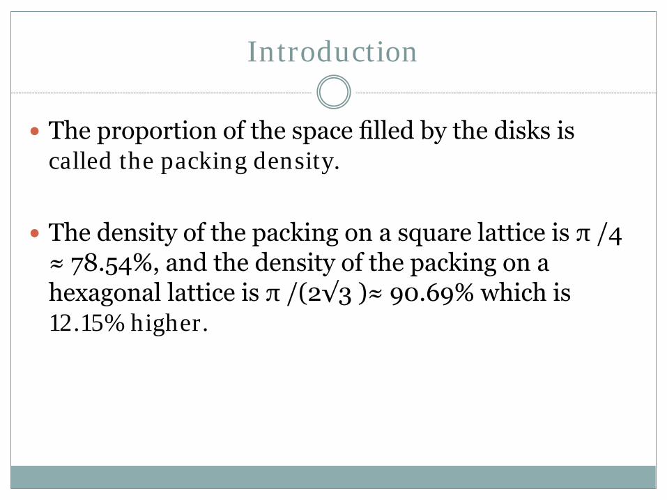
The proportion of the space filled by the disks is called the packing density.

The density of the packing on a square lattice is π /4 ≈ 78.54%, and the density of the packing on a hexagonal lattice is π /(2√3 )≈ 90.69% which is 12.15% higher.

Advantages of Hexagonal Lattices

More uniform distribution of lattice points

Each lattice point has six equidistant neighbors

Allow efficiently indexed regular hexagonal structures which approximate circular regions better than square structures

2. CT image reconstruction

For a 2D object, CT image reconstruction uses the 3 major steps to reconstruct the image of the scanned object:a). 1D fast Fourier transform (FFT) of the projection to build a polar 2D Fourier space using the Fourier slice theorem; b). polar to Cartesian resampling; c). filtered backprojection (FBP) method , or apply inverse 2D FFT to obtain the reconstructed image.

projection

1D FT

objectx

y

u

v D FT of1anotherprojections

2D IFT

ts

θ

Fourier slice theorem: The 1D FT of a projection taken at angle θ equals the

central radial slice at angle θ of the 2D FT of the original object.

For the convenience of computations involving rotations, the input image is assumed to be circular upon zero paddings.

The frequencies from the back projections in different angles also occupy a circular region.

2. CT image reconstruction continue

Frequencies after projections, and the reconstructed image

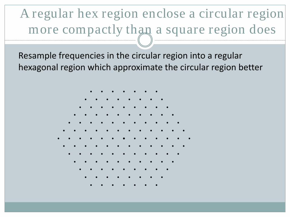
A regular hex region enclose a circular region more compactly than a square region does

Resample frequencies in the circular region into a regular hexagonal region which approximate the circular region better

Apply FBP or inverse FFT on the hexagonal structure

3. Advantages of optimal lattices and efficient domains for reconstruction and segmentation

Higher packing density, higher degree of circular symmetry, more uniform connectivity

Mersereau showed that for signals which are band-limited over a circular region, 13.4% fewer samples are required to maintain equal high frequency image information with the rectangular grid.

In 2014, Hofmann and Tiede published results on image segmentation, and concluded that hexagonal sampling grids have advantages on better shape representation of image objects.

We tested the following 4 images for reconstruction on hex and square lattices

Reconstruction effect on hex lattice vs square lattice

For any of the last 4 images, based on the 2-norm criterion, the reconstruction effect on a hexagonal lattice is better than the effect on the square lattice with the same sampling density

The least square error of the reconstruction on a hexagonal lattice is about one-half of the least square error on the square lattice with the same sampling density

Knaup applied hexagonal lattices for image reconstruction over a square region as below

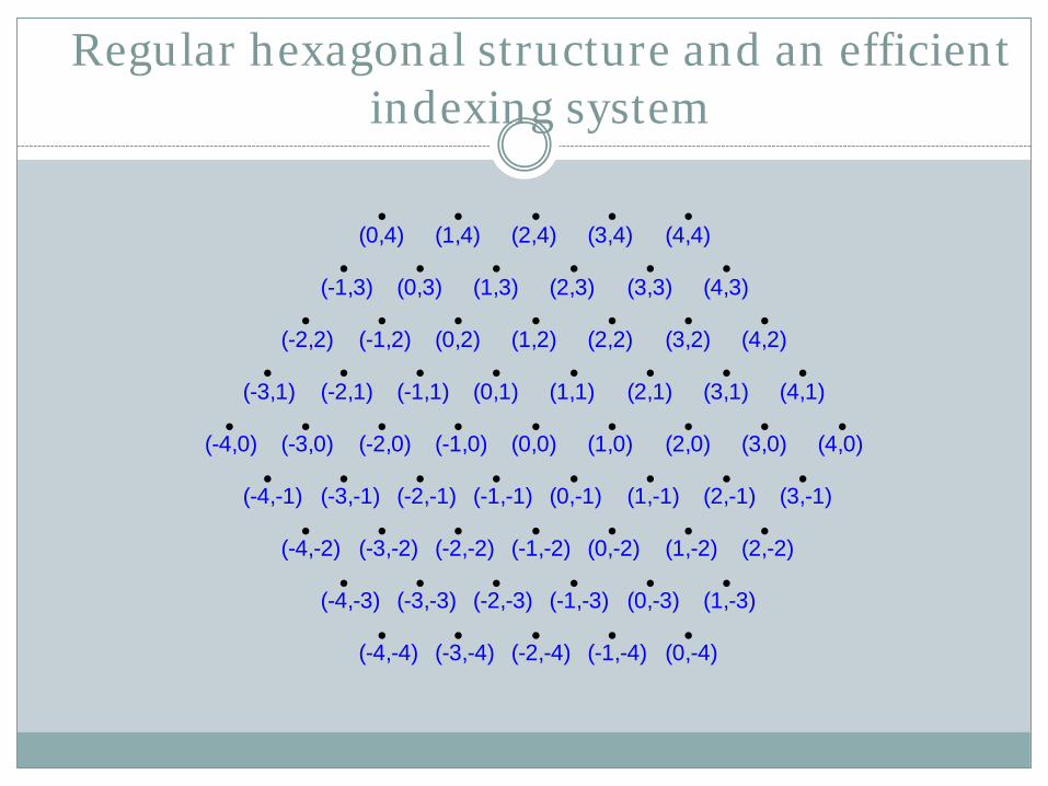
Regular hexagonal structure and an efficient indexing system

(-4,-4)

(-4,-3)

(-4,-2)

(-4,-1)

(-4,0)

(-3,-4)

(-3,-3)

(-3,-2)

(-3,-1)

(-3,0)

(-3,1)

(-2,-4)

(-2,-3)

(-2,-2)

(-2,-1)

(-2,0)

(-2,1)

(-2,2)

(-1,-4)

(-1,-3)

(-1,-2)

(-1,-1)

(-1,0)

(-1,1)

(-1,2)

(-1,3)

(0,-4)

(0,-3)

(0,-2)

(0,-1)

(0,0)

(0,1)

(0,2)

(0,3)

(0,4)

(1,-3)

(1,-2)

(1,-1)

(1,0)

(1,1)

(1,2)

(1,3)

(1,4)

(2,-2)

(2,-1)

(2,0)

(2,1)

(2,2)

(2,3)

(2,4)

(3,-1)

(3,0)

(3,1)

(3,2)

(3,3)

(3,4)

(4,0)

(4,1)

(4,2)

(4,3)

(4,4)

Image reconstruction over the regular hexagonal structure

For the same sampling density, the number of lattice points of a regular hexagonal structure is just about 87% of the number of lattice points of a square structure. Hence the CT reconstruction time will be reduced if the reconstruction is done on the regular hexagonal domain instead of the square domain.

From the figure shown in the last slide, we can see that the regular hexagonal structure has an efficient indexing system. Furthermore, the neighbors of each lattice point can be determined easily based on the index of that lattice point.

Image segmentation

Image segmentation is to partition an image into regions corresponding to the actual objects so that the size and geometry of the objects can be easily determined.

Graph partitioning methods are effective tools for image segmentation since they model the impact of pixel neighborhoods on a given cluster of pixels or pixel, under the assumption of homogeneity in images.

Contour of the liver segmentation (in red) compared to the original CT scan slice

The regular hexagonal structure is very suitable for image segmentation

Because the number of lattice points of a regular hexagonal structure is just about 87% of the number of lattice points of a square structure, the image segmentation time will be reduced if the reconstruction is done on the regular hexagonal domain instead of the square domain.

Because the neighbors of each lattice point in a regular hexagonal structure can be determined easily based on the index of that lattice point, the use of a regular hexagonal structure is convenient to the graph cut method for image segmentation.

The three dimensional case

The 3-dimensional optimal sampling lattices are face centered cubic (FCC) and body centered cubic (BCC) lattices.

In 2014, Zheng and Gu published a paper entitled fast Fourier transform on FCC and BCC lattices with outputs on FCC and BCC lattices respectively

The following truncated octahedron structure was shown in the paper by Zheng and Gu in 2014. The number of lattice points of this structure is about 77% of the number of lattice points of a cubic structure to enclose the same ball.

Truncated octahedron structure versus the cubic structure

For the same sampling density, the number of lattice points of the truncated octahedron structure is about 77% of the number of lattice points of a cubic structure to enclose the same ball. Hence the CT reconstruction time will be reduced if we use the truncated octahedron domain instead of the cubic domain.

As shown in the paper by Zheng and Gu, we can see that the truncated octahedron structure has an efficient indexing system. Furthermore, the neighbors of each lattice point can be determined easily based on the index of that lattice point.

4. Possible application of optimal sampling lattices on some 3D printing tasks

Because FCC lattices have higher packing density than 3D Cartesian lattices, if we use an FCC lattice to coordinate the ceramic printing, then the printed object may have better precision and has a smoother surface.

We may develop efficient computer algorithms for 3D printing utilizing optimal sampling lattices.

Ceramic objects printed by Daniel De Bruin

The left is a cubic lattice voxel and the right is a FCC voxel in Kaloian Petkov's thesis

In a paper by Ye and Entezari, visual comparison of images rendered from the Cartesian, BCC, and FCC lattices

corresponding to the following 1st, 2nd, and 3rd figure

5. Summary and tentative future research topics

We have shown the advantages of some optimal sampling lattices and efficient domains for CT image reconstruction. We have also shown the possible application of optimal sampling lattices in some 3D printing tasks such as the printing of some ceramic objects.

In the future, we will try to do simulations or to collaborate with other researchers to do experiments.

Questions?

References:1. Vince and X. Zheng, Computing the discrete Fourier transform on a lattice, Journal of Mathematical Imaging and Vision, Vol. 28, pp. 125--133, 2007.

2. X. Zheng and F. Gu, Fast Fourier transform on FCC and BCC lattices with outputs on FCC and BCC lattices respectively, Journal of Mathematical Imaging and Vision, Vol. 49, pp. 530—550, 2014.