Application of Plantwide Control to the HDA Process.I - Steady-State Optimization and Self-Optimizing

Control

Antonio Araujo a Marius Govatsmarka Sigurd Skogestada,1

aDepartment of Chemical EngineeringNorwegian University of Science and Technology

N-7491 Trondheim, Norway

Abstract

This paper describes the application of self-optimizing control to a large-scale process, theHDA plant. The idea is to select controlled variables which when kept constant lead to min-imum economic loss. First, the optimal active constraints need to be controlled. Next, con-trolled variables need to be found for the remaining unconstrained degrees of freedom. Inorder to avoid the combinatorial problem related to the selection of outputs/measurementsfor such large plants, a local (linear) analysis based on singular value decomposition (SVD)is used for pre-screening. This is followed by a more detailed analysis using the nonlinearmodel. Note that a steady-state model, in this case one builtin Aspen PlusTM , is sufficientfor selecting controlled variables. A dynamic model is required to design and test the com-plete control system which include regulatory control. This is considered in the part II ofthe series.

Key words:HDA process, self-optimizing control, selection of controlled variable, Aspen PlusTM .

1 Introduction

This paper deals with the selection of controlled variablesfor the HDA process.One objective is to avoid the combinatorial control structure issue for such large-scale processes by using local methods based on the singularvalue decompositionof the linearized model of the process.

1 Corresponding author: E-mail: sigurd.skogestad@chemeng.ntnu.no. Fax: +47-7359-4080

Preprint submitted to Elsevier 30 October 2006

The selection of controlled variables is based on steady-state economics and usethe ideas of self-optimizing control to find the best set(s).Self-optimizing controlis when an acceptable (economic) loss can be achieved using constant set pointsfor the controlled variables, without the need to reoptimize when disturbances oc-cur (Skogestad, 2000). The constant set point policy is simple but will not be op-timal (and thus have a positive loss) as a result of the following two factors: (1)disturbances, i.e., changes in (independent) variables and parameters that cause theoptimal set points to change, and (2) implementation errors, i.e., differences be-tween the setpoints and the actual values of the controlled variables (e.g., becauseof measurement errors or poor control). The effect of these factors (or more specif-ically the loss) depends on the choice of controlled variables, and the objective isto find a set of controlled variables for which the loss is acceptable.

The HDA process (Figure 1) was first presented in a contest which the AmericanInstitute of Chemical Engineers arranged to find better solutions to typical designproblems (McKetta, 1977). It has been exhaustively studiedby several authors withdifferent objectives, such as steady-state design, controllability and operability ofthe dynamic model and control structure selection and controller design.

Mixer FEHE Furnace PFR Quench

Separator

Compressor

Cooler

StabilizerBenzeneColumn

TolueneColumn

H2 + CH4

Toluene

Toluene Benzene CH4

Diphenyl

Purge (H2 + CH4)

Mixer FEHE Furnace PFR Quench

Separator

Compressor

Cooler

StabilizerBenzeneColumn

TolueneColumn

H2 + CH4

Toluene

Toluene Benzene CH4

Diphenyl

Purge (H2 + CH4)

Fig. 1. HDA process flowsheet.

This paper is organized as follows: Section 2 examines previous proposed controlstructures for the HDA process. Section 3 shortly introduces the self-optimizingcontrol technique. Section 4 describes the HDA process and the features of themodel used in the present article. Section 5 summarizes the results found by apply-ing the self-optimizing control procedure and the SVD analysis to the selection ofcontrolled variables for the HDA process. A discussion of the results is found inSection 6 followed by a conclusion in Section 7.

2

2 Previous work on the HDA process

Stephanopoulos (1984) followed the approach proposed by Buckley (1964) basedon material balance and product quality control. He used an HDA plant modelwhere steam is generated from the effluent of the feed effluentheat exchangerthrough a series of steam coolers. From the material balanceviewpoint, the se-lected controlled variables of choice were fresh toluene feed flow rate (productionrate control), recycle gas flow rate, hydrogen contents in the recycle gas, purge flowrate, and quencher flow rate. Product quality is controlled through product compo-sitions in the distillation columns and the controlled variables selected are productpurity in benzene column and reactor inlet temperature.

Later, Douglas (1988) used another version of the HDA process to demonstrate asteady-state procedure for flowsheet design.

Brognaux (1992) implemented both a steady-state and dynamic model of the HDAplant in SpeedupTM based on the model developed by Douglas (1988) and used itas an example to compute operability measurements, define control objectives, andperform controllability analysis. He found that it is optimal to control the activeconstraints found by optimization.

Wolff (1994) used an HDA model based on Brognaux (1992)) to illustrate a pro-cedure for operability analysis. He concluded that the HDA process is controllableprovided the instability of the heat-integrated reactor isresolved. After some addi-tional heuristic consideration, the controlled variableswere selected to be the sameas used by Brognaux (1992).

Ng and Stephanopoulos (1996) used the HDA process to illustrate how plantwidecontrol systems can be synthesized based on a hierarchical framework. The selec-tion of controlled variables is performed somehow heuristically by prioritizing theimplementation of the control objectives. In other words, it is necessary to controlthe material balances of hydrogen, methane and toluene, theenergy balance is con-trolled by the amount of energy added to the process (as fuel in the furnace, coolingwater, and steam), production rate, and product purity.

Caoet al. used the HDA process as a case study in several papers, but mainly tostudy input selection, whereas the focus of the present paper is on output selection.In Cao and Biss (1996), Cao and Rossiter (1997), Caoet al. (1997a), and Cao andRossiter (1998) issues involving input selection are discussed. Caoet al. (1997b)considered input and output selection for control structure design purposes usingthe singular value decomposition (SVD). Caoet al. (1998a) applied a branch andbound algorithm based on local (linear) analysis. All the papers by Caoet al.utilizethe same controlled variables selected heuristically by Wolff (1994). Caoet al.(1998b) discuss the importance of modelling in order to achieve themost effectivecontrol structure and improves the HDA process model for such purpose.

3

Ponton and Laing (1993) presented a unified heuristic hierarchical approach to pro-cess and control system design based on the ideas of Douglas (1988) and usedthe HDA process throughout. The controlled variables selected at each stage are:Toluene flow rate, hydrogen concentration in the reactor, and methane contents inthe compressor inlet (feed and product rate control stage);separator liquid streamoutlet temperature and toluene contents at the bottom of thetoluene column (re-cycle structure, rates and compositions stage); and separator separator pressure,benzene contents at stabilizer overhead, and toluene contents at benzene columnoverhead are related to product and intermediate stream composition stage. Thestages related to energy integration and inventory regulation do not cover the HDAprocess directly, so no controlled variables are assigned at these stages.

Luybenet al.(1998) applied a heuristic nine-step procedure together with dynamicsimulations to the HDA process and concluded that control performance is worsewhen the steady-state economic optimal design is used. Theychose to control theinventory of all components in the process (hydrogen, methane, benzene, toluene,and diphenyl) to ensure that the component material balanceare satisfied; the tem-peratures around the reactor are controlled to ensure exothermic heat removal fromthe process; total toluene flow or reactor inlet temperature(it is not exactly clearwhich one was selected) can be used to set production rate andproduct purity bythe benzene contents in the benzene column distillate. Luyben (2002) uses therigorous commercial flowsheet simulators HysysTM , Aspen PlusTM and AspenDyanmicsTM to propose a heuristic-based control structure for the HDA process.

Herrmannet al. (2003) consider the HDA process to be an important test-bedproblem for design of new control structures due to its high integration and non-minimum phase behavior. They re-implemented Brognaux (1992)’s model in As-pen Custom ModelerTM and design a model-based, multivariableH∞ controller forthe process. They considered the same controlled variablesused by Wolff (1994).

Kondaet al. (2005) used an integrated framework of simulation and heuristics andproposed a control structure for the HDA process. A HysysTM model of the plantwas built to assist the simulations. They selected fresh toluene feed flow rate to setproduction rate, product purity at benzene column distillate to fulfill the productspecification, overall toluene conversion in the reactor toregulate the toluene recy-cle loop, ratio of hydrogen to aromatics and quencher outlettemperature to fulfillprocess constraint, and methane contents in the purge stream to avoid its accumu-lation in the process.

Table 1 summarizes the selection of (steady-state) controlled variables by variousauthors. It seems clear that the systematic selection of controlled variable for thisplant has not been fully investigated although the process has been extensivelyconsidered by several authors. In this work, a set(s) of controlled variables for theHDA process is to be systematically selected.

4

Table 1Steady-state controlled variables selected by various authors.

Stephanopoulos (1984)Brognaux (1992), Wolff (1994), Cao et al., and Herrmann et al. (2003)Ng and Stephanopoulos (1996)Ponton and Laing (1993)Luyben et al. (1998) and Luyben (2002)Konda et al. (2005)This work

Number of steady-state (economic) controlled variables1 8 7 6 8 8 9 13

Y202 Fresh toluene feed rate (active constraint)3 x x x xY71 Recycle gas flow rate xY48 Recycle gas hydrogen mole fraction xY49 Recycle gas methane mole fraction x x x xY62 Reactor inlet pressure (active constraint) xY68 Compressor power x x x x x xY72 Total toluene flow rate to the reaction section xY28 Mixer outlet hydrogen mole fraction xY5 Reactor inlet temperature x x xY19 Separator temperature (active constraint) x x x xY64 Separator pressure x x x xY70 Hydrogen to aromatics ratio at the reactor inlet (active constraint) x x xY73 Hydrogen mole fraction in the reactor outlet xY69 Overall toluene conversion in the reactor xY27 Quencher flow rate xY16 Quencher outlet temperature (active constraint) x x xY26 Purge flow rate xY46 Separator liquid toluene mole fraction xY74 Hydrogen mole fraction in stabilizer distillate xY53 Benzene mole fraction in stabilizer distillate x xY54 Methane mole fraction in stabilizer bottoms xY55 Benzene product purity (active constraint) x x x x x xY56 Benzene mole fraction in benzene column bottoms xY75 Production rate (benzene column distillate flow rate) xY76 Temperature in an intermediate stage of the benzene column xY77 Temperature in an intermediate stage of the toluene column xY78 Toluene mole fraction in toluene column distillate x xY58 Toluene mole fraction in toluene column bottoms xY57 Diphenyl mole fraction in toluene column distillate x

1 The total number of steady-state degrees of freedom is13, so there are additional controlled variables, or fixed inputs,

which are not clearly specified by some authors.2 Y-variables refer to candidates in Table 4.3 Active constraints found in this work.

3 Selection of controlled variables using self-optimizing control

The selection of primary controlled variables is considered here. The objective isto achieve self-optimizing control where fixing the primarycontrolled variablescat constant setpointscs indirectly leads to near-optimal operation (see Figure 2).

More precisely (Skogestad, 2004):

Self-optimizing control is when one can achieve an acceptable loss with constantsetpoint values for the controlled variables without the need to re-optimize whendisturbances occur.

5

Fig. 2. Typical control hierarchy in a chemical plant.

For continuous processes with infrequent grade chages, like the HDA process, asteady-state analysis is usually sufficient because the economics can be assumed tobe determined by the steady-state operation.

It is assumed that the optimal operation of the system can be quantified in termsof a scalar cost function (performance index)J0, which is to be minimized withrespect to the available degrees of freedomu0

minu0

J0(x, u0, d) (1)

subject to the constraints

g1(x, u0, d) = 0; g2(x, u0, d) ≤ 0 (2)

Hered represents all of the disturbances, including exogenous changes that affectthe system (e.g., a change in the feed), changes in the model (typically representedby changes in the functiong1), changes in the specifications (constraints), andchanges in the parameters (prices) that enter in the cost function and the constraints.x represents the internal variables (states). One way to approach this problem is toevaluate the cost function for the expected set of disturbances and implementationerrors. The main steps of this procedure are as follows (Skogestad, 2000):

1. Degree of freedom analysis.

6

2. Definition of optimal operation (cost and constraints).3. Identification of important disturbances (typically, feed flow rates, active con-

straints and input error).4. Optimization.5. Identification of candidate controlled variablesc.6. Evaluation of loss for alternative combinations of controlled variables (loss

imposed by keeping constant set points when there are disturbances or imple-mentation errors), including feasibility investigation.

7. Final evaluation and selection (including controllability analysis).

To achieve optimal operation, the active constraints are chosen to be controlled.The difficult issue is to decide which unconstrained variablesc to control.

Unconstrained problem: The original independent variablesu0 = u′, u are di-vided into the “constraint” variablesu′ (used to satisfy the active constraintsg′

2 = 0)and the remaining unconstrained variablesu. The value ofu′ is then a function ofthe remaining independent variables (u andd). Similarly, the statesx are deter-mined by the value of the remaining independent variables. Thus, by solving themodel equations (g1 = 0), and for the active constraints (g′

2 = 0), one may for-mally write x = x(u, d) andu′ = u′(u, d) and one may formally write the cost asa function ofu andd: J = J0(x, u0, d) = J0[x(u, d), u′(u, d), u, d] = J(u, d). Theremaining unconstrained problem in reduced space then becomes

minu

J(u, d) (3)

whereu represents the set of remaining unconstrained degrees of freedom. Thisunconstrained problem is the basis for the local method introduced below.

3.1 Degrees of freedom analysis

It is paramount to determine the number of steady-state degrees of freedom becausethis in turns determines the number of steady-state controlled variables that needto be chosen. To find them for complex plants, it is useful to sum the number ofdegrees for individual units as given in Table 2 (Skogestad,2002).

3.2 Local (linear) method

In terms of the unconstrained variables, the loss function around the optimum canbe expanded:

7

Table 2Typical number of steady-state degrees of freedom for some process units.

Process unit DOF

Each external feed stream 1 (feedrate)

Splitter n − 1 split fractions (n is the number ofexit streams)

Mixer 0

Compressor, turbine, and pump 1 (work)

Adiabatic flash tank 0∗

Liquid phase reactor 1 (holdup)

Gas phase reactor 0∗

Heat exchanger 1 (duty or net area)

Columns (e.g. distillation) excluding heatexchangers

0∗ + number of side streams

∗ Add 1 degree of freedom for each extra pressure that is set (need anextra valve, compres-sor, or pump), e.g. in flash tank, gas phase reactor, or column.

L = J(u, d) − Jopt(d) =1

2‖z‖2

2 (4)

with z = J1/2uu (u − uopt) = J1/2

uu G−1(c − copt), whereG is the steady-state gainmatrix from the unconstrained degrees of freedomu to the controlled variablesc(yet to be selected) andJuu the Hessian of the cost function with respect to theu.Truly optimal operation corresponds toL = 0, but in generalL > 0. A small valueof the loss functionL is desired as it implies that the plant is operating close to itsoptimum. The main issue here is not to find the optimal set points, but rather to findthe right variables to keep constant.

Assuming that each controlled variableci is scaled such that||e′c|| = ||c′−c′opt||2 ≤1, the worst case loss is given by (Halvorsenet al., 2003):

Lmax = max||ec||2≤1

L =1

2

1

σ(S1GJ−1/2uu )2

(5)

whereS1 is the matrix of scalings forci:

S1 = diag{1

span(ci)} (6)

wherespan(ci) = ∆ci,opt(d) + ni (∆ci,opt(d) is the variation ofci due to variationin disturbances andni is the implementation error ofci)

8

It may be cumbersome to obtain the matrixJuu, and if it is assumed that each “basevariable”u has been scaled such that a unit change in each input has the same effecton the cost functionJ (such that the HessianJuu is a scalar times unitary matrix,i.e.Juu = αU), then (5) becomes

Lmax =α

2

1

σ(S1G)2(7)

whereα = σ(Juu).

Thus, to minimize the lossL σ(S1GJ−1/2uu ) should be maximized or alternatively

maximizeσ(S1G); the latter is the original minimum singular value rule of Sko-gestad (2000).

Originally, a MatLabTM model was used to obtain the optimal variation∆copt(d),the steady-state gain matrixG and the HessianJuu, but in the present version AspenPlusTM is used instead (see the Appendix for details). The use of a commercialflowsheet simulator like Aspen PlusTM demonstrates the practical usefulness ofthe approach.

4 HDA process description

In the HDA process, fresh toluene (pure) and hydrogen (97% hydrogen and3%methane) are mixed with recycled toluene and hydrogen (Figure 1). This reactantmixture is first preheated in a feed-effluent heat exchanger (FEHE) using the reactoreffluent stream and then to the reaction temperature in a furnace before being fedto an adiabatic plug-flow reactor.

A main reaction and a side reaction take place in the reactor as follows:

Toluene + H2 → Benzene + Methane (8)2 Benzene Diphenyl + H2 (9)

The reactor effluent is quenched by a portion of the recycle separator liquid flowto prevent coking, and further cooled in the FEHE and cooler before being fed tothe vapor-liquid separator. Part of the vapor containing unconverted hydrogen andmethane is purged to avoid accumulation of methane within the process while theremainder is compressed and recycled to the process. The liquid from the separatoris processed in the separation section consisting of three distillation columns. Thestabilizer column removes small amounts of hydrogen and methane in the overheadproduct, and the benzene column takes of the benzene productin the overhead.

9

Finally, in the toluene column, unreacted toluene is separated from diphenyl andrecycled to the process.

4.1 Details of the HDA process model in Aspen PlusTM

The model of the HDA process used in this paper is a modified version of the modeldeveloped by Luyben (2002). A schematic flowsheet of the Aspen PlusTM modelis depicted in Figure 3 and the corresponding stream table isshown in Table 3.

10

FFH2

2

28

29

27F1

LIQ

15

GREC

TOTTOL 8

22

23

18

19

GAS

31

12

32 RIN

ROUT

13

PURGE

TREC

FFTOL

D1

B1

5

D2

B2

17

D3

B3

3

30

9

3326

V1

V6

V4

P1

T2

T1

T3COMP

HX

FURRX

COND

V5

SEP

V10

V3

QUENCHER

T5

C1 C2

C3

V12

V11

V14

V13

V15

P3

P5

P2

P4

HDA Process

Fig. 3. HDA Aspen PlusTM process flowsheet.

11

Table 3Stream table for the nominally optimal operating point for the HDA process. See Figure 3 for the stream names.Stream 2 7 8 9 12 13 14 15 17 18 19 20 21 22 23 26 27 28 29 30Mole Flow (lbmol/h)

Hydrogen 433.19 1.0817 1807.4 0 1517.8 1517.8 0 1.7588 0 1516141.75 0 0 0 0 0 1.0817 0.6771 0.6771 0Methane 13.398 14.42 2910.2 0 3219.1 3219.1 0 23.446 0 3195.6298.79 0 0 0 0 0 14.42 9.0263 9.0263 0Benzene 0 3.2877 45.09 273.02 498.97 498.97 267.99 449.27 5.0297 49.705 4.6475 267.99 5.0297 0 5.0297 1E-06 276.31 172.96 172.96 1E-06Toluene 0 0.011 316.39 15.551 26.314 26.314 0.0101 25.303 15.541 1.0111 0.0945 0.0101 15.541 300 15.541 4E-05 15.562 9.7413 9.7413 4E-05Diphenyl 0 0 0.0105 9.4543 15.376 15.376 0 15.372 9.4543 0.0031 0.0003 0 9.4543 0 1.4544 8 9.4543 5.9181 5.9181 8

Mole Fraction Hydrogen 0.97 0.0575 0.3559 0 0.2876 0.2876 0 0.0034 0 0.31830.3183 0 0 0 0 0 0.0034 0.0034 0.0034 0Methane 0.03 0.767 0.573 0 0.61 0.61 0 0.0455 0 0.671 0.671 0 0 0 0 0 0.0455 0.0455 0.0455 0Benzene 0 0.1749 0.0089 0.9161 0.0945 0.0945 0.9997 0.8721 0.1675 0.0104 0.0104 0.9997 0.1675 0 0.2284 1E-07 0.8721 0.8721 0.8721 1E-07Toluene 0 0.0006 0.0623 0.0522 0.005 0.005 4E-05 0.0491 0.5176 0.0002 0.0002 4E-05 0.5176 1 0.7056 6E-06 0.0491 0.0491 0.0491 6E-06Diphenyl 0 0 2E-06 0.0317 0.0029 0.0029 0 0.0298 0.3149 6E-076E-07 0 0.3149 0 0.066 0.99999 0.0298 0.0298 0.0298 0.99999

Total Flow (lbmol/h) 446.59 18.8 5079.2 298.02 5277.5 5277.5 268 515.15 30.025 4762.4 445.28 268 30.025 300 22.025 8 316.82 198.32 198.32 8Temperature (F) 100.11 199.97 120.25 235.29 357.62 95 223.9 95.381 306.72 124.91 124.91 224.01 299.51 100.27 275.5 567.05 95.381 95.381 95.607 565.91Pressure (psi) 575 50 530 31.714 476 476 80 530 84 555 555 50 30.75 575 575 82 530 530 486 32Vapor Fraction 1 1 0.932 0.4558 1 0.9024 0 0 0 1 1 0 0.0314 0 0 0 0 0 0 0.0057Enthalpy (MBtu/h) -0.355 -0.32 -88.22 9.705 -68.63 -90.327.038 10.046 0.9862 -99.2 -9.275 7.038 0.9862 1.8366 0.444 0.6787 6.1787 3.8677 3.8677 0.6787

Stream 31 32 B1 B2 B3 D1 D2 D3 F1 FFH2 FFTOL GAS GREC LIQ PURGE RINROUT TOTTOL TRECMole Flow (lbmol/h)

Hydrogen 1517.8 1807.4 0 0 0 1.0817 0 0 1.0817 433.19 0 1516 1374.3 1.7588 141.75 1807.4 1517.1 0 0Methane 3219.1 2910.2 0 0 0 14.42 0 0 14.42 13.398 0 3195.6 2896.8 23.446 298.79 2910.2 3210.1 0 0Benzene 498.97 45.09 273.02 5.0297 1E-06 3.2877 267.99 5.0297 276.31 0 0 49.705 45.058 449.27 4.6475 45.09 326.01 0.03255.0297Toluene 26.314 316.39 15.551 15.541 4E-05 0.011 0.0101 15.541 15.562 0 300 1.0111 0.9166 25.303 0.0945 316.39 16.573 315.47 15.541Diphenyl 15.376 0.0105 9.4543 9.4543 8 0 0 1.4544 9.4543 0 0 0.0031 0.0028 15.372 0.0003 0.0105 9.4572 0.0078 1.4544

Mole Fraction Hydrogen 0.2876 0.3559 0 0 0 0.0575 0 0 0.0034 0.97 0 0.3183 0.3183 0.0034 0.3183 0.3559 0.2987 0 0Methane 0.61 0.573 0 0 0 0.767 0 0 0.0455 0.03 0 0.671 0.671 0.0455 0.671 0.573 0.632 0 0Benzene 0.0945 0.0089 0.9161 0.1675 1E-07 0.1749 0.9997 0.2284 0.8721 0 0 0.0104 0.0104 0.8721 0.0104 0.0089 0.0642 0.0001 0.2284Toluene 0.005 0.0623 0.0522 0.5176 6E-06 0.0006 4E-05 0.7056 0.0491 0 1 0.0002 0.0002 0.0491 0.0002 0.0623 0.0033 0.99990.7056Diphenyl 0.0029 2E-06 0.0317 0.3149 0.99999 0 0 0.066 0.02980 0 6E-07 6E-07 0.0298 6E-07 2E-06 0.0019 2E-05 0.066

Total Flow (lbmol/h) 5277.5 5079.2 298.02 30.025 8 18.8 268 22.025 316.82 446.59 300 4762.4 4317.1 515.15 445.28 5079.2 5079.2 315.51 22.025Temperature (F) 1150 1004.9 371.42 306.34 565.91 205.55 223.51 270.17 98.003 100 100 95 124.91 95 123.87 1201.2 1277.2 110.48 275.16Pressure (psi) 486 510 154 34 32 150 30 30 160 625 625 476 555 476 505 500 500 575 675Vapor Fraction 1 1 0 0 0 1 0 0 0.0293 1 0 1 1 0 1 1 1 0 0Enthalpy (MBtu/h) -7.29 -26.88 9.705 0.9853 0.6778 -0.32 7.0323 0.4367 6.1787 -0.355 1.8366 -100.4 -89.93 10.036 -9.275 -11.16 -11.16 2.0586 0.444

12

Details on this model can be found in Luyben (2002). The main difference betweenthe model in this paper and Luyben’s lies on the distillationtrain. As optimizationof the entire plant is difficult for this problem, it has been decided to first optimizethe distillation train separately (see Section 5.4.1). Thedistillation train may thenbe represented by simple material balances with given specifications. This was im-plemented in Aspen PlusTM using an ExcelTM spreadsheet, and optimization of theremaining plant is then relatively simple.

5 Results

This section describes the self-optimizing control procedure applied to the HDAprocess model in Aspen PlusTM starting with the degree of freedom analysis.

5.1 Step 1. Degree of freedom analysis

It is considered 20 manipulated variables (Table 6), 70 candidate measurements(the first 70 in Table 4), and 12 disturbances (Table 8). The 20manipulated vari-ables correspond to 20 dynamic degrees of freedom. However,at steady state thereare only 13 degrees of freedom because there are 7 liquid levels that need to becontrolled which have no steady-state effect. This is confirmed by the alternativesteady-state degree of freedom analysis in Table 5.

With 13 degrees of freedom and 70 candidate controlled variables, there are(

7013

)

=70!

13!57!= 4.7466·1013 (!) control structures, without including the alternativeways of

controlling liquid levels. Clearly, an analysis of all of them is intractable. To avoidthis combinatorial explosion, the active constraints are first determined, which shouldbe controlled to achieve optimal operation, and then a localanalysis to eliminatefurther sets is applied.

5.2 Step 2. Definition of optimal operation

The following profit function (−J) [M$/year] given by Douglas (1988)’s economicpotential (EP) is to be maximized:

(−J) = (pbenDben +nc∑

i=1

pf,iFf,i) − (ptolFtol + pgasFgas + pfuelQfuel +

pcwQcw + ppowWpow + pstmQstm) (10)

subject to the constraints

13

Table 4Selected candidate controlled variables for the HDA process (excluding levels).

Y1 Mixer outlet temperature Y22 Mixer outlet flow rate

Y2 FEHE hot side outlet temperature Y23 Quencher outlet flow rate

Y3 Furnace inlet temperature Y24 Separator vapor outlet flow rate

Y4 Furnace outlet temperature Y25 Separator liquid outlet flow rate

Y5 Rector section 1 temperature Y26 Purge flow rate

Y6 Rector section 2 temperature Y27 Flow of cooling stream to quencher

Y7 Rector section 3 temperature Y28 Mixer outlet hydrogen mole fraction

Y8 Rector section 4 temperature Y29 Mixer outlet methane mole fraction

Y9 Rector section 5 temperature Y30 Mixer outlet benzene mole fraction

Y10 Rector section 6 temperature Y31 Mixer outlet toluene mole fraction

Y11 Rector section 7 temperature Y32 Mixer outlet diphenyl mole fraction

Y12 Rector section 8 temperature Y33 Quencher outlet hydrogen molefraction

Y13 Rector section 9 temperature Y34 Quencher outlet methane mole frac-tion

Y14 Rector section 10 temperature Y35 Quencher outlet benzene mole frac-tion

Y15 Rector section 11 temperature Y36 Quencher outlet toluene mole frac-tion

Y16 Quencher outlet temperature (activeconstraint)

Y37 Quencher outlet diphenyl mole frac-tion

Y17 Compressor inlet temperature Y38 Separator overhead vapor hydrogenmole fraction

Y18 Compressor outlet temperature Y39 Separator overhead vapor methanemole fraction

Y19 Separator temperature (active con-straint)

Y40 Separator overhead vapor benzenemole fraction

Y20 Fresh toluene feed rate (active con-straint)

Y41 Separator overhead vapor toluenemole fraction

Y21 Fresh gas feed flow rate Y42 Separator overhead vapor diphenylmole fraction

14

Table 4Selected candidate controlled variables for the HDA process (excluding levels) (cont’).

Y43 Separator liquid outlet hydrogenmole fraction

Y61 Furnace inlet pressure

Y44 Separator liquid outlet methanemole fraction

Y62 Reactor inlet pressure (active con-straint)

Y45 Separator liquid outlet benzene molefraction

Y63 Reactor outlet pressure

Y46 Separator liquid outlet toluene molefraction

Y64 Separator pressure

Y47 Separator liquid outlet diphenylmole fraction

Y65 Compressor outlet pressure

Y48 Gas recycle hydrogen mole fractionY66 Furnace heat duty

Y49 Gas recycle methane mole fraction Y67 Cooler heat duty

Y50 Gas recycle benzene mole fraction Y68 Compressor power

Y51 Gas recycle toluene mole fraction Y69 Toluene conversion at reactor outlet

Y52 Gas recycle diphenyl mole fraction Y70 Hydrogen to aromatic ratio in reac-tor inlet (active constraint)

Y53 Benzene mole fraction in stabilizerdistillate (active constraint)

Y71 Recycle gas flow rate

Y54 Methane mole fraction in stabilizerbottoms (active constraint)

Y72 Total toluene flow rate to the reac-tion section

Y55 Benzene mole fraction in benzenecolumn distillate (active constraint)

Y73 Hydrogen mole fraction in the reac-tor outlet

Y56 Benzene mole fraction in benzenecolumn bottoms (active constraint)

Y74 Hydrogen mole fraction in stabilizerdistillate

Y57 Diphenyl mole fraction in toluenecolumn distillate (active constraint)

Y75 Production rate (benzene columndistillate flow rate)

Y58 Toluene mole fraction in toluenecolumn bottoms (active constraint)

Y76 Temperature in an intermediatestage of the benzene column

Y59 Mixer outlet pressure Y77 Temperature in an intermediatestage of the toluene column

Y60 FEHE hot side outlet pressure Y78 Toluene mole fraction in toluenecolumn distillate

15

Table 5Steady-state degrees of freedom analysis based on Table 2.

Process unit DOF

External feed streams 2 · 1 = 2

Splitters (purge and quench) 2 · 1 = 2

Compressor 1 · 1 = 1

Adiabatic flash(∗) (quencher and separator) 2 · 0 = 0

Gas phase reactor(∗) 1 · 0 = 0

Heat exchangers in recycle section(∗∗) (furnace and cooler) 2 · 1 = 2

Heat exchangers in 3 distillation columns 3 · 2 = 6

Total 13(∗) Assuming no adjustable valves for pressure control (assumefully open valve beforeseparator).(∗∗) The FEHE (feed effluent heat exchanger) duty is not a degree offreedom becausethere is no adjustable bypass.

1. Minimum production rate

Dbenzene ≥ 265 lbmol/h (11)

2. Hydrogen to aromatic ratio in reactor inlet (to prevent coking)

FH2

(Fbenzene + Ftoluene + Fdiphenyl)≥ 5 (12)

3. Maximum toluene feed rate

Ftoluene ≤ 300lbmol/h (13)

4. Reactor inlet pressure

Preactor,in ≤ 500 psia (14)

5. Reactor outlet temperature

Treactor,out ≤ 1300oF (15)

6. Quencher outlet temperature

Tquencher,out ≤ 1150oF (16)

7. Product purity at the benzene column distillate

xD,benzene ≥ 0.9997 (17)

16

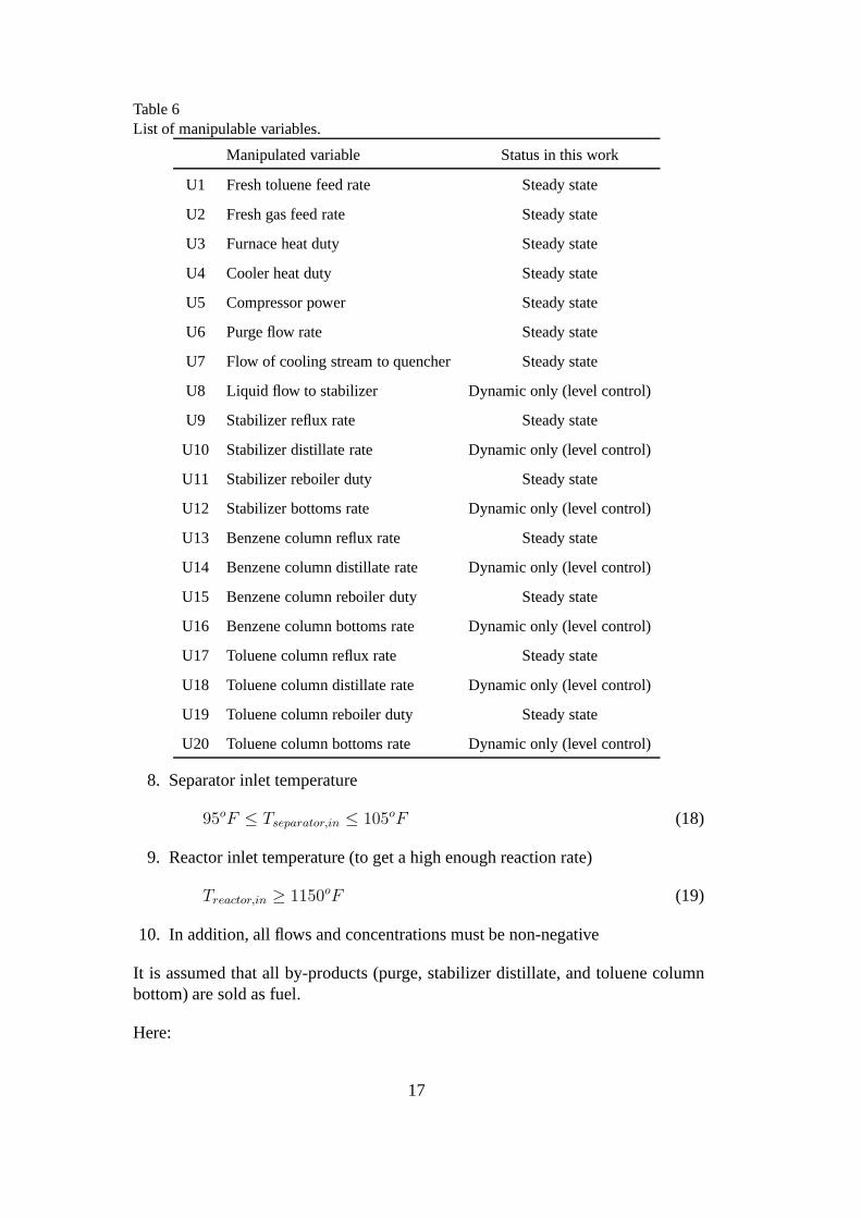
Table 6List of manipulable variables.

Manipulated variable Status in this work

U1 Fresh toluene feed rate Steady state

U2 Fresh gas feed rate Steady state

U3 Furnace heat duty Steady state

U4 Cooler heat duty Steady state

U5 Compressor power Steady state

U6 Purge flow rate Steady state

U7 Flow of cooling stream to quencher Steady state

U8 Liquid flow to stabilizer Dynamic only (level control)

U9 Stabilizer reflux rate Steady state

U10 Stabilizer distillate rate Dynamic only (level control)

U11 Stabilizer reboiler duty Steady state

U12 Stabilizer bottoms rate Dynamic only (level control)

U13 Benzene column reflux rate Steady state

U14 Benzene column distillate rate Dynamic only (level control)

U15 Benzene column reboiler duty Steady state

U16 Benzene column bottoms rate Dynamic only (level control)

U17 Toluene column reflux rate Steady state

U18 Toluene column distillate rate Dynamic only (level control)

U19 Toluene column reboiler duty Steady state

U20 Toluene column bottoms rate Dynamic only (level control)

8. Separator inlet temperature

95oF ≤ Tseparator,in ≤ 105oF (18)

9. Reactor inlet temperature (to get a high enough reaction rate)

Treactor,in ≥ 1150oF (19)

10. In addition, all flows and concentrations must be non-negative

It is assumed that all by-products (purge, stabilizer distillate, and toluene columnbottom) are sold as fuel.

Here:

17

1. pben, ptol, pgas, pfuel, pcw, ppow, andpstm are the prices of benzene, freshtoluene feed, fresh gas feed, fuel to the furnace, cooling water, power to thecompressor, and steam, respectively (see Table 7 for data);

2. Dben, Ftol, Fgas, Qfuel, Qcw, Wpow, andQstm are the flows of product ben-zene, fresh toluene feed, fresh gas (hydrogen) feed, fuel tothe furnace, coolingwater, power to the compressor, and steam, respectively;

3. Qcw = Qcw,cooler + Qcw,stab + Qcw,ben−col + Qcw,tol−col;4. Qstm = Qstm,stab + Qstm,ben−col + Qstm,tol−col;5. Ff,i = Fpurge,i + Dstab,i + Btol−col,i, i = 1, ..., nc (nc is the number of com-

ponents in the system), whereFpurge is the flow through the purge,Dstab,i isthe flow through the stabilizer distillate, andBtol−col,i is the flow through thetoluene column bottom;

6. pf,i is the price associated toFf,i, i = 1, ..., nc.7. 8150 hours of operation per year.

Table 7Economic data for the HDA process based on Douglas (1988).

pben 9.04$/lbmol

ptol 6.04$/lbmol

pgas 1.32$/lbmol

pfuel 4.00 · 10−6$/Btu

pcw 23.42 · 10−3$/Btu

ppow 0.042$/bhp

pstm 2.50 · 10−6$/Btu

5.3 Step 3. Identification of important disturbances

The 12 disturbances listed in Table 8 are considered. They include changes in thefeed and in the active constraints.

5.4 Step 4. Optimization

5.4.1 Optimization of the distillation columns

The six steady-state degrees of freedom for the three distillation columns shouldideally be used to optimize the profit for the entire plant, but as mentioned inSection 4, a simplified recovery model is used for the distillation columns whenmodeling the entire plant to make the optimization feasible. The error imposedby this is expected to be very small. The distillation columns were therefore opti-mized separately using detailed models. Assumed internal prices were defined to

18

Table 8Disturbances to the process.

Nominal Disturbance

D1 Fresh toluene feed rate [lbmol/h] 300 285

D2 Fresh toluene feed rate [lbmol/h] 300 315

D3 Fresh gas feed rate methane mole fraction 0.03 0.08

D4 Hydrogen to aromatic ratio in reactor inlet 5.0 5.5

D5 Reactor inlet pressure [psi] 500 520

D6 Quencher outlet temperature [oF] 1150 1170

D7 Product purity in the benzene column distillate 0.9997 0.9960

D8 Benzene mole fraction in stabilizer distillate 1 · 10−4 3 · 10−4

D9 Methane mole fraction in stabilizer bottoms 1 · 10−6 5 · 10−6

D10 Benzene mole fraction in benzene column bottoms1.3 · 10−3 2 · 10−3

D11 Diphenyl mole fraction in toluene column distillate0.5 · 10−3 1 · 10−3

D12 Toluene mole fraction in toluene column bottoms 0.4 · 10−3 1 · 10−3

take care of the interaction with the remaining process. Fordistillation columns,to avoid product give-away, it is always optimal to have the most valuable productat its constraint. In the present case, there is only one product constraint, namelyxD,benzene ≥ 0.9997, and this should always be active as benzene is the main (andmost valuable) product. For the remaining distillation products, the optimal con-ditions were obtained by a trade-off between maximizing therecovery of valuablecomponent and minimizing energy (favored by a large mole fraction). Figure 4shows the relations between the reboiler duty and the respective mole fraction ofvaluable component for each distillation column. When the mole fraction is lessthan about10−3, its economic effect on the recovery is small. In general, a goodtrade-off is achieved if there is a small mole fraction (about 10−3 or less) in the“flat” region.

The resulting “optimal” values for the five remaining degrees of freedom (productcompositions) are given in Table 9.

The reason why the impurities in Table 9 are so small is that the columns in thispaper have many stages so that it does not cost much energy to achieve higherpurity. This also means that the optimal point is “flat” (which is good) as it is alsoillustrated by Figure 5. For the stabilizer column, the separation is very simple andimproving the purity has almost no penalty in terms of reboiler duty.

Note that it has been chosen to use product compositions as controlled variables(specifications) for the distillation columns. There are two reasons for this: First,

19

10−7

10−6

10−5

10−4

10−33.7618

3.7618

3.7619

3.762

3.762

3.762

3.7621

3.7622

3.7622

3.7622

3.7623x 106

xD,benzene

Qre

boile

r [Btu

/h]

(a)

xB,methane

= 1 ⋅ 10−6

10−6

10−5

10−4

10−3

10−20

1

2

3

4

5

6

7

8

9

10x 107

xB,benzene

Qre

boile

r [Btu

/h]

(b)

xB,benzene

= 1.3⋅10−3

10−6

10−5

10−4

10−30

1

2

3

4

5

6

7

8

9

10x 106

xB,toluene

Qre

boile

r [Btu

/h]

(c)

xD,diphenyl

= 5⋅10−4

Fig. 4. Typical relations between reboiler duty and productpurity. (a) Stabilizer distillate;(b) Benzene column bottoms; (c) Toluene column bottoms.

20

Table 9Specifications for distillation columns.

Column/Specification Value Comment

Stabilizer

Y53 xD,benzene 1 · 10−4 (A)

Y54 xB,methane 1 · 10−6 (B)

Benzene column

Y55 xD,benzene 0.9997 Active constraint

Y56 xB,benzene 1.3 · 10−3 (A)

Toluene column

Y57 xD,diphenyl 0.5 · 10−3 (C)

Y58 xB,toluene 0.4 · 10−3 (A)

(A) Determined by trade-off between energy usage and recovery (Figure 4).

(B) xB,methane should be small to avoid methane impurity in distillate of benzene column.

(C) Diphenyl should not be recycled because it may reduce theavailable production rate if there is bottleneck in the plant.

with fixed product compositions only mass balances are needed to represent thedistillation columns when simulating the overall process in Aspen PlusTM . Sec-ond, compositions are good self-optimizing variables in most cases (e.g. Skogestad(2000)). also note that the product compositions should normally be given in termsof impurity of key components (Luybenet al., 1998) as this avoids problems withnon-unique specifications.

These six specifications for the distillation columns consumes six steady-state de-grees of freedom. There are then13 − 6 = 7 degrees of freedom left.

5.4.2 Optimization of the entire process (reactor and recycle)

Optimization with respect to the7 remaining steady-state degrees of freedom wasperformed using an SQP algorithm in Aspen PlusTM . Figure 5 gives the effect ofdisturbances on the profit(−J). Note that disturbances D8 - D12 in the distilla-tion product compositions have almost no effect. This is expected,,since the fivedistillation composition specifications (Table 9) are in the “flat” region and havepractically no influence in the profit. A change in the given purity for the benzeneproduct (disturbance D7) has, as expected, a quite large effect. The detailed resultsfor disturbances D1 to D7 are summarized in Table 10.

From Table 10, 5 constraints are optimally active in all operating points:

21

D5(0.60%)

D4(2.28%)

D3(0.95%)

D8(0.00%)

D9(0.01%)

D10(0.00%)

D12(0.01%)

D11(0.02%)

Nominal

D6(0.66%) D7

(0.32%)

D2(4.47%)

D1(3.00%)

4,50

4,55

4,60

4,65

4,70

4,75

4,80

4,85

4,90

4,95

Pro

fit

[M$/

year

]

Fig. 5. Effect of disturbances (see Table 8) on optimal operation. Percentages in parenthesesare changes with respect to the nominal optimum.

Y16. Quencher outlet temperature (upper bound)Y19. Separator temperature (lower bound)Y20. Fresh toluene feed rate (upper bound)Y62. Reactor inlet pressure (upper bound)Y70. Hydrogen to aromatic ratio in reactor inlet (lower bound)

As expected, the benzene purity at the outlet of the process is kept at its boundfor economic reasons. Moreover, fresh feed toluene is maintained at its maximumflow rate to maximize the profit. The separator inlet temperature is kept at its lowerbound in order to maximize the recycle of hydrogen and to avoid the accumulationof methane in the process. Luyben’s rule of keeping all recycle loops under flowcontrol is not economically optimal in this process since itis best to let the recycleflow fluctuates.

All the 5 active constraints should be controlled to achieve optimaloperation (Maarleveldand Rijnsdorp, 1970). Consequently, the remaining number of unconstrained de-grees of freedom is2 (7 − 5 = 2). This reduces the number of possible sets ofcontrolled variables to

(

592

)

= 59!2!57!

= 1, 711, where the number59 is found bysubtracting from the initial70 candidate measurements in Table 4 the6 distillationspecifications and5 active constraints of the reactor and recycle process. However,this number is still too large to consider all alternatives in detail.

The next step uses local analysis to find promising candidatesets of2 controlledvariables.

22

Table 10Effect of disturbances on optimal values for selected variables.

Variable Unit Nominal D1 D2 D3 D4 D5 D6 D7

Profit k$/year 4,693.4 4,552.7 4,903.2 4,649.0 4,585.6 4,664.7 4,722.5 4,705.5

Y4 oF 1201.15 1198.20 1202.89 1204.66 1206.66 1196.44 1201.88 1199.33

Y15 oF 1277.21 1273.64 1279.25 1277.71 1279.65 1272.25 1276.89 1274.99

Y16(∗) oF 1150 1150 1150 1150 1150 1150 1170 1150

Y19(∗) oF 95 95 95 95 95 95 95 95

Y20(∗) lbmol/h 300 285 315 300 300 300 300 300

Y21 lbmol/h 446.59 431.29 470.33 476.29 460.03 446.75 444.73 445.46

Y26 lbmol/h 445.27 429.78 468.91 474.95 458.44 445.27 443.23 443.90

Y28 0.3558 0.3548 0.3577 0.3454 0.3703 0.3558 0.3526 0.3560

Y29 0.5729 0.5742 0.5707 0.5854 0.5622 0.5730 0.5767 0.5727

Y45 0.8721 0.8671 0.8703 0.8667 0.8792 0.8683 0.8692 0.8662

Y46 0.0491 0.0544 0.0511 0.5419 0.4534 0.5322 0.5205 0.5549

Y49 0.6710 0.6717 0.6691 0.6803 0.6534 0.6708 0.6737 0.6705

Y53(∗∗) 1 · 10−4 1 · 10−4 1 · 10−4 1 · 10−4 1 · 10−4 1 · 10−4 1 · 10−4 1 · 10−4

Y54(∗∗) 1 · 10−6 1 · 10−6 1 · 10−6 1 · 10−6 1 · 10−6 1 · 10−6 1 · 10−6 1 · 10−6

Y55(∗∗) 0.9997 0.9997 0.9997 0.9997 0.9997 0.9997 0.9997 0.996

Y56(∗∗) 1.3 · 10−3 1.3 · 10−3 1.3 · 10−3 1.3 · 10−3 1.3 · 10−3 1.3 · 10−3 1.3 · 10−3 1.3 · 10−3

Y57(∗∗) 5 · 10−4 5 · 10−4 5 · 10−4 5 · 10−4 5 · 10−4 5 · 10−4 5 · 10−4 5 · 10−4

Y58(∗∗) 4 · 10−4 4 · 10−4 4 · 10−4 4 · 10−4 4 · 10−4 4 · 10−4 4 · 10−4 4 · 10−4

Y62(∗) psi 500 500 500 500 500 520 500 500

Y68 hp 454.39 443.20 474.93 473.22 485.53 564.09 460.82 455.41

Y70(∗) 5.0 5.0 5.0 5.0 5.5 5.0 5.0 5.0

(∗) Active constraints.(∗∗) Distillation specification.

5.5 Step 5. Identification of candidate controlled variables - local analysis

A branch-and-bound algorithm (Caoet al., 1998a) for maximizing the minimumsingular value ofS1GJ−1/2

uu andS1G was used to obtain the candidate sets of con-trolled variables (details on the calculation ofS1, G, andJuu are given in the Ap-pendix). Note that the steady-state gain matrixG is obtained with the5 activeconstraints fixed at their optimal values. The minimum singular value of the16candidate sets are given in Table 12 and the15 (out of 59) measurements involvedin the16 sets are listed in Table 11, with their nominally optimal values, the opti-mal variations, and assumed implementation errors (i.e, the total span is the sum ofthe optimal variation and the implementation error). From Table 12 it is seen thatthe same best10 sets were identified for both criteria of maximizingσ(S1GJ−1/2

uu )andσ(S1G). Also note the10 best sets all include the reactor feed inert (methane)mole fraction (Y29) plus another composition (of benzene, toluene, or diphenyl)as controlled variable. The remaining6 sets (XI - XVI) are some other commonchoices that are reasonable to consider, including inert (methane) recycle concen-tration (Y49), the furnace outlet temperature (Y4), the purge rate (Y26), and the

23

compressor power (Y68). Set XII with fixed furnace outlet temperature (Y4) andinert (methane) concentration (Y49) is similar to the structure of Luyben (2002),although Luyben does not control all the active constraints.

Table 11Candidate controlled variables with small losses in local analysis.

Variable Name Nominal Optimal Implementation Total

optimal variation error span

Y4 Furnace outlet temperature 1201.15 5.52 60.06 65.57

Y26 Purge flow rate 445.27 29.73 22.26 52

Y29 Mixer outlet inert (methane) mole fraction 0.5729 0.0125 0.0001 0.0126

Y30 Mixer outlet benzene mole fraction 0.0091 0.000068 0.0001 0.000168

Y35 Quencher outlet benzene mole fraction 0.0996 0.0059 0.0001 0.006

Y36 Quencher outlet toluene mole fraction 0.0031 0.0007 0.0001 0.0008

Y37 Quencher outlet diphenyl mole fraction 0.0033 0.0003 0.0001 0.0004

Y40 Separator overhead vapor benzene mole fraction 0.0107 0.000081 0.0001 0.000181

Y45 Separator liquid benzene mole fraction 0.8721 0.0071 0.0001 0.0072

Y46 Separator liquid toluene mole fraction 0.0491 0.0071 0.0001 0.0072

Y47 Separator liquid diphenyl mole fraction 0.0318 0.0023 0.0001 0.0024

Y49 Gas recycle inert (methane) mole fraction 0.6710 0.0175 0.0001 0.0176

Y50 Gas recycle benzene mole fraction 0.0107 0.000081 0.0001 0.000181

Y68 Compressor power 454.39 109.69 4.54 114.23

Y69 Toluene conversion at reactor outlet 0.9124 0.0076 0.01 0.0176

Table 12Local analysis: Minimum singular values for candidate setsof unconstrained controlledvariables.

Set Variable 1 Variable 2 1000 · σ(S1G2×2) 1000 · σ(S1G2×2J−1/2uu )

Full(∗) 6.2523 6.3436

I Y29 Y36 2.2942 2.3331

II Y29 Y69 2.2523 2.2761

III Y29 Y45 2.2133 2.2545

IV Y29 Y46 2.2102 2.2398

V Y29 Y40 2.2072 2.2201

VI Y29 Y50 2.1981 2.2199

VII Y29 Y35 1.8452 1.8247

VIII Y29 Y47 1.8344 1.8044

IX Y29 Y30 1.7855 1.7851

X Y29 Y37 1.7149 1.6825

XI Y4 Y26 1.2439 1.2815

XII Y4 Y49 0.2008 0.1957

XIII Y26 Y49 1.3352 1.2902

XIV Y4 Y68 0.1198 0.1201

XV Y26 Y68 1.2196 1.2785

XVI Y49 Y68 0.0198 0.0201

(∗) With all 59 variables:Gfull = G59×2.

24

5.6 Step 6. Detailed evaluation of the loss

The next step is to evaluate the loss for the promising sets ofcontrolled variablesin Table 12 by keeping constant setpoint policy when there are disturbances and/orimplementation errors. The computations were performed onthe nonlinear modelin Aspen PlusTM for disturbances D1 through D7 (the losses for disturbancesD8to D12 are negligible, as discussed above) and the results are shown in Table 13.

Table 13Loss in k$/year caused by disturbances and implementation errors forthe alternative setsof controlled variables from Table 12.

Set D1 D2 D3 D4 D5 D6 D7 ny1(∗) ny2 Average

I 70.40 5.37 14.41 4.57 12.85 12.57 9.66 5.33 3.37 15.39

II 86.16 10.91 25.78 18.98 27.11 13.31 17.77 5.33 33.58 26.55

III 100.01 13.22 35.40 26.66 55.52 13.60 21.82 5.33 10.92 31.39

IV 118.45 16.04 38.22 39.52 60.30 37.98 43.17 5.33 4.57 40.40

V 136.60 16.92 48.46 53.16 69.07 41.48 78.59 5.33 16.17 51.75

VI 143.54 19.70 48.47 58.17 79.12 51.23 106.07 5.33 12.02 58.18

VII 149.94 22.01 58.42 67.39 79.27 64.68 112.07 5.33 12.05 63.46

VIII 140.83 23.40 59.81 85.09 81.44 76.60 118.25 5.33 12.03 66.97

IX 150.37 25.25 67.70 96.31 83.30 85.55 136.07 5.33 3.40 72.59

X 151.61 31.07 70.11 99.91 88.29 106.15 141.18 5.33 4.19 77.54

XI 163.29 43.10 97.70 133.87 104.15 127.00 150.84 243.97 176.86 137.87

XII (∗∗) 188.09 55.86 125.35 169.45 128.55 151.18 178.46 243.97 25.46 140.71

XIII 162.78 37.49 88.99 144.73 128.55 124.42 148.47 176.86 25.46 115.31

XIV 193.80 61.99 131.70 157.08 137.96 154.38 188.23 243.97 302.04 174.57

XV 179.48 43.24 89.21 183.32 155.35 122.78 159.47 176.86 302.04 156.86

XVI 233.26 188.87 259.70 364.56 186.68 171.82 224.66 25.46 302.04 217.45

(∗) ny1 andny2 are the implementation errors associated with each variable in the set.(∗∗) This is similar to the structure of Luyben (2002), but with control of active constraints.

As seen in Tables 12 and 13, the results from the linear and nonlinear analysis givethe same ranking for the sets of candidate controlled variables, with the best setshaving both the largest value ofσ(S1G2×2J

−1/2uu ) (as one would expect from (7))

and the lowest value of the actual loss. Note from Table 13 that all the structureswere found to be feasible for the given disturbances.

Compared to the controlled structure proposed by Luyben (2002) the sets of con-trolled variables selected by the self-optimizing controlapproach give smaller eco-nomic losses. This is because the steady-state nominal point of Luyben (2002) is notoptimal: It gives a profit of(−J) = 3.955.2 k$/year, which is about16% smallerthan the nominally optimal operation (4, 693.4k$/year) found in this paper. First,Luyben (2002) considers only12 degrees of freedom at steady state as compres-sor power is assumed fixed. Second, Luyben (2002) does not control all the activeconstraints in the process. Specifically, the hydrogen-to-aromatics ratio, which isan important variable in the process and should be kept at itslower bound of5 (see

25

(12)), is not controlled. Instead, Luyben (2002) controls inert (methane) composi-tion in the recycle gas and reactor inlet temperature which results in large economiclosses.

6 Discussion

In this paper, it has been considered the standard operationmode with given feedrate (indirectly, through an upper bound on toluene feed). Yet another importantmode of operation is maximum throughput, which occurs when prices are such thatit is optimum to maximize production.

Another point to stress is the consistency of the results with the empirical argu-ments made by Douglas (1988) which is that impurity levels should be controlledin order to avoid build-up of inerts in the system that eventually makes the processinoperable. This was accomplished when the inert (methane)concentration leavingthe mixer (controlled variable Y29 above) was chosen to be controlled.

The final evaluation and selection of the control structure involves the selection ofsets of controlled variables with acceptable loss, such as those shown in Table 13.These are then analyzed to see if they are adequate with respect to the expected dy-namic control performance (input-output controllability). This, in addition to max-imum throughput case and design of the regulatory layer, will be the focus of partII of the series where a dynamic analysis is used.

7 Conclusions

This paper has discussed the selection of controlled variables for the HDA processusing the self-optimizing control procedure. The large number of variable combi-nations makes it a challenging problem, and a local (linear)analysis based on theSVD of the linearized model of the plant was used to select good candidate sets forthe unconstrained controlled variables. Specifically,16 candidate sets were foundto be suitable to select from. Aspen PlusTM proved to be a valuable tool for theevaluation of self-optimizing control structures for large-scale processes.

8 Appendix

This appendix outlines the steps taken to compute the steady-state linear matrixGand the HessianJuu of the unconstrained inputs as well as the optimal variationforthe candidate variablesspan(ci).

26

Optimization of the entire plant in Aspen PlusTM was used to identify the activeconstraints. For the local analysis (calculation of∆copt(d), G, andJuu), several aux-iliary blocks were used, including a Calculator block to compute the value of thecost function; Design Specification blocks were used to close feedback loops forthe active constraints; and a Sensitivity block was used to perform auxiliary compu-tations. Finally, Aspen PlusTM was used to compute the “nonlinear” loss imposedby keeping the selected sets of controlled variables constant at their setpoints.

8.1 Calculation of the linear matrixG and the HessianJuu

G andJuu are calculated with respect to the nominal optimal operating point, i.e.for d = 0. The matrixG is calculated by the usual approximation:

∂ci(u)

∂uj

= limh→0

c(u + ejh) − c(u)

hj

(20)

wherei = 1...nc is the index set of candidate variables,j = 1...nu is the indexset of unconstrained inputs,h is the vector of increments for each inputuj, andej = [000...1...0] is the zero vector except for the j-element which is1.

In Aspen PlusTM , c(u) andc(u + ejh) are evaluated by adding the stepejh to thevectoru for each inputj in a Calculator block and then taken the resulting vectorsto a MatLabTM code that numerically calculates the termsGij = ∂ci(u)

∂uj.

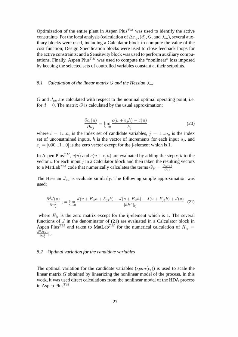
The HessianJuu is evaluate similarly. The following simple approximationwasused:

∂2J(u)

∂u2j

|i = limh→0

J(u + Eiih + Ejjh) − J(u + Eiih) − J(u + Ejjh) + J(u)

[hhT ]ij(21)

whereEij is the zero matrix except for the ij-element which is1. The severalfunctions ofJ in the denominator of (21) are evaluated in a Calculator block inAspen PlusTM and taken to MatLabTM for the numerical calculation ofHij =∂2J(u)

∂u2j|i.

8.2 Optimal variation for the candidate variables

The optimal variation for the candidate variables (span(ci)) is used to scale thelinear matrixG obtained by linearizing the nonlinear model of the process.In thiswork, it was used direct calculations from the nonlinear model of the HDA processin Aspen PlusTM .

27

For each candidate controlled variableci, it is obtained its maximum optimal vari-ation ∆ci,opt(d) due to variation in disturbances. From the nonlinear model,theoptimal parameters (inputs and outputs) for various conditions (disturbances andoperating points) are computed. This yields a “lookup” table of optimal parametervalues as a function of the operating conditions. From this,one can identify:

∆ci,opt(d) = maxj∈D

(|cji,opt − cnom

i,opt|) (22)

whereD is the set of disturbances,cji,opt is the optimal value ofci due to disturbance

j andcnomi,opt is the nominal optimal value ofci.

For each candidate controlled variableci, its expected implementation errorni (sumof measurement error and control error) is obtained. Then, the candidate controlledvariables are scaled such that for each variablei the sum of the magnitudes of∆ci,opt(d) and the implementation errorni is similar, which corresponds to select-ing the scaling:

span(ci) = ∆ci,opt(d) + ni (23)

Then, the scaling matrixS1 can be computed asS1 = diag{ 1span(ci)

}. All data were

retrieved from nonlinear simulations in Aspen PlusTM and the calculations wereperformed in a dedicated MatLabTM code.

References

Brognaux, C. (1992). A case study in operability analysis: TheHDA plant. Master thesis.University of London, London, England.

Buckley, P. S. (1964).Techniques of process control. John Wiley and Sons. New York,USA.

Cao, Y. and D. Biss (1996). New screening techniques for choosing manipulated variables.In: Preprints IFAC ’96, 13th World Congress of IFAC, Volume M. San Francisco, CA.

Cao, Y. and D. Rossiter (1997). An input pre-screening technique for control structureselection.Computers and Chemical Engineering21(6), 563–569.

Cao, Y. and D. Rossiter (1998). Input selection and localized disturbance rejection.Journalof Process Control8(3), 175–183.

Cao, Y., D. Rossiter and D. Owens (1997a). Input selection for disturbance rejectionunder manipulated variable constraints.Computers and Chemical Engineering21(Suppl.), S403–S408.

28

Cao, Y., D. Rossiter and D. Owens (1997b). Screening criteria for input and outputselection. In: Proceedings of European Control Conference, ECC 97. Brussels,Belgium.

Cao, Y., D. Rossiter and D. Owens (1998a). Globally optimal control structure selectionusing branch and bound method. In:Proceedings of DYCOPS-5, 5th IFAC Symposiumon Dynamics and Control of Process Systems. Corfu, Greece.

Cao, Y., D. Rossiter, D.W. Edwards, J. Knechtel and D. Owens (1998b). Modellingissues for control structure selection in a chemical process. Computers and ChemicalEngineering22(Suppl.), S411–S418.

Douglas, J. M. (1988).Conceptual Design of Chemical Processes. McGraw-Hill. USA.

Halvorsen, I J., S. Skogestad, J. C. Morud and V. Alstad (2003). Optimal selection ofcontrolled variables.Ind. Eng. Chem. Res.42, 3273–3284.

Herrmann, G., S. K. Spurgeon and C. Edwards (2003). A model-based sliding mode controlmethodology applied to the hda-plant.Journal of Process Control13, 129–138.

Konda, N. V. S. N. M., G. P. Rangaiah and P. R. Krishnaswamy (2005). Simulation basedheuristics methodology for plant-wide control of industrial processes. In:Proceedingsof 16th IFAC World Congress. Praha, Czech Republic.

Luyben, W. L. (2002).Plantwide dynamic simulators in chemical processing and control.Marcel Dekker, Inc.. New York, USA.

Luyben, W. L., B. D. Tyreus and M. L. Luyben (1998).Plantwide process control.McGraw-Hill. USA.

Maarleveld, A. and J. E. Rijnsdorp (1970). Constraint control on distillation columns.Automatica6, 51–58.

McKetta, J. J. (1977).Benzene design problem. Encyclopedia of Chemical Processing andDesign. Dekker, New York, USA.

Ng, C. and G. Stephanopoulos (1996). Synthesis of control systems for chemical plants.Computers and Chemical Engineering20, S999–S1004.

Ponton, J.W. and D.M. Laing (1993). A hierarchical approachto the design of processcontrol systems.Trans IChemE71(Part A), 181–188.

Skogestad, S. (2000). Plantwide control: The search for theself-optimizing controlstructure.Journal of Process Control10, 487–507.

Skogestad, S. (2002). Plantwide control: Towards a systematic procedure. In:Proceedingsof the European Symposium on Computer Aided Process Engineering 12. pp. 57–69.

Skogestad, S. (2004). Near-optimal operation by self-optimizing control: from processcontrol to marathon running and business systems.Computers and ChemicalEngineering29(1), 127–137.

Stephanopoulos, G. (1984).Chemical process control. Prentice-Hall International Editions.New Jersey, USA.

29

Wolff, E. A. (1994). Studies on control of integrated plants. PhD thesis. NorwegianUniversity of Science and Technology, Trondheim, Norway.

30