11
25
†To whom correspondence should be addressed.
E-mail: [email protected]
Korean J. Chem. Eng., 29(1), 25-35 (2012)DOI: 10.1007/s11814-011-0130-5
INVITED REVIEW PAPER
Application of simulated annealing (SA) to the synthesis of heterogeneous catalytic reactor
Sungwon Hwang*,† and Robin Smith**
*Process, Technology and Engineering, UOP Ltd., Liongate, Ladymead, Guildford, Surrey, GU1 1AT, UK**Centre for Process Integration, School of Chemical Engineering and Analytical Science,
The University of Manchester, P. O. Box 88, Manchester, M60 1QD, UK(Received 3 April 2011 • accepted 11 May 2011)
Abstract−This paper reviews a practical application of the optimization algorithm to conceptual design of a heteroge-
neous catalytic reactor and catalyst and its synthesis. In particular, a simulated annealing (SA) algorithm is mainly used
since it provides a reliable optimization solution without being trapped at local optimum points, which arise from non-
convexities and multiplicities in a complex reaction system. Furthermore, it allows a design engineer to evaluate multiple
design options of reactor and catalyst systems which satisfy both user-specified objective functions and constraints.
In the final stage of optimization, these generated solutions are fine-tuned by using deterministic optimization. To enhance
the efficiency of optimization further, a profile-based synthesis is adopted for the optimization algorithm. Lastly, this
research takes into account a number of factors for the synthesis of heterogeneous catalytic reactors such as reactor
configuration, uniform and non-uniform catalyst type, and fundamental catalyst design parameters including shape
and its definite dimensions.
Key words: Catalyst, Reactor, Optimization, Simulated Annealing, Modelling
INTRODUCTION
Many different types of optimization algorithms have been devel-
oped and applied to systematic process design in chemical engi-
neering. Each optimization algorithm has its own advantages and
disadvantages, and it is essential to understand the nature of each
algorithm and to ensure if an appropriate tool is employed for the
system design. In broad terms, optimization can be divided into two
different categories: deterministic and stochastic optimization. The
most well-known algorithm of deterministic optimization is succes-
sive quadratic programming (SQP) for non-linear problems, whilet
various stochastic optimizations have been developed such as sim-
ulated annealing, genetic algorithms, neural networks, tabu search,
and target analysis.
Deterministic algorithms such as successive quadratic program-
ming (SQP) can in principle find a global optimization solution very
fast for a continuous and non-linear problem. However, limitations
arise when the problem belongs to MINLP (mixed integer non-linear
programming) models. Furthermore, these conventional determin-
istic optimization methods show frequent traps to local optimal points
in a highly non-linear problem of reactor synthesis.
In the present study, simulated annealing (SA), which utilizes
stochastic optimization, is used for the synthesis of reactor and hetero-
geneous catalyst. The main advantage of using this stochastic algo-
rithm is that the global optimization point can be reached regardless
of the initial starting point, since the algorithm incorporates proba-
bilistic elements both in the problem and algorithm itself in contrast
to deterministic optimization. Furthermore, the algorithm provides
various design solutions that satisfy the objective function and con-
straints. Therefore, various types of novel reactor and catalyst designs
can be developed from the optimization results. However, this method
suffers from a relatively large computation time for the optimiza-
tion compared with deterministic algorithms. For this reason, an
innovative approach is used in this work to maximize the use of
powerful functions of these two individual algorithms. For exam-
ple, a simulated annealing (SA) method is mainly used at initial stage
of optimization to find a set of feasible optimum solutions, while
the obtained premature solutions are fine-tuned by using a SQP (suc-
cessive quadratic programming) algorithm at final stage. Further-
more, a profile-based synthesis approach is adopted in order to in-
crease the efficiency of the optimization algorithm further.
For illustration, the modelling of a non-uniform catalyst and its
synthesis with a heterogeneous catalyst reactor in ethylene oxida-
tion process is represented.
BACKGROUNDS
1. Simulated Annealing (SA)
As defined in its name, simulated annealing exploits the basic
concept from the process of metal annealing. Physical metal anneal-
ing is a process of transforming from high energy in liquid to low
energy status in a solid by initially melting the substance and de-
creasing temperature slowly, spending long time near the freezing
point. In the liquid state, particles are distributed randomly. How-
ever, a stable crystalline state is formed with a minimum energy
configuration corresponding to the one of the solid. In the process
of annealing, the solid cannot reach the minimum energy status if
the cooling is not done slowly enough, and it becomes unstable like
a glass or a crystal with several defects in the structure. Further-
more, the resulting solids at different energy conditions of the simu-
lated annealing method refer to different feasible solutions in the

26 S. Hwang and R. Smith
January, 2012
combinatorial optimization problem, and the energy of the solid
corresponds to the objective function, which is to be minimized.
The approach of simulated annealing is based on simple algo-
rithm of Metropolis et al., which originally introduced the methods
to find the equilibrium configuration of a collection of atoms at a
given temperature [1]. The connection between this algorithm and
mathematical minimization was first noted by Pincus and Kirkpatrick
et al. who proposed the optimization technique for combinatorial
problems [2,3]. Since then, simulated annealing has been applied
to various optimization problems in areas such as computer design,
image screening, molecular physics, chemistry, process design, and
so on [4]. Apart from simulated annealing, other heuristic search
methods have also been developed, such as genetic algorithms, neural
networks, tabu search and target analysis. These heuristic search
methods are summarized by Glover and Greenberg [5]. These opti-
mization methods produce good solutions but not necessarily a global
optimum solution, within a reasonable computing time. Simulated
annealing has also been extended to optimization problems with
continuous variables, and the summary of these approaches can be
found in the work of Van Laarhoven and Aarts [6].
The major advantage of simulated annealing is an ability to avoid
being trapped at a local optimum point during optimization. The
algorithm employs a random search accepting not only the change
that improves the objective function but also the changes that deteri-
orate it.
2. Logical Theory of Simulated Annealing (SA)
Simulated annealing is a modification of a local search algo-
rithm. A brief procedure of local search algorithm follows.
1. Select an initial state at i and calculate f(i).
2. Generate neighbor, j, in a random manner and calculate f(j).
3. Calculate δ (=f(j)−f(i)), comparing current result with previ-
ous result.
4. Replace the result if the current result is better than previous
result.
5. Repeat steps 2 to 4.
6. Stop.
Even though this local search algorithm is simple and quick to
execute, the main disadvantage of this method is that the solution
might be far from any global optimum point. A possible solution
to this problem is to exploit multiple starting points to produce dif-
ferent optimum results, and the best optimum solution among the
resulting products can be regarded as a global optimum point. In a
similar approach, the simulated annealing avoids being trapped in
a local optimum point by sometimes accepting the neighbors, pro-
ducing results which go in the opposite direction of the optimum
point. The acceptance or rejection of these opposite moves is deter-
mined by a sequence of random numbers but with a controlled prob-
ability. The probability of acceptance for the move, which goes away
from the optimum point, is called the acceptance function. It is gen-
erally set to exp(−δ/T), where T is a cooling temperature. In princi-
ple, a small increase of the objective function of f is more likely to
be accepted than a large increase, for example, in the case of minimi-
zation of f. Also, most moves are accepted at a high temperature,
while most increase moves are rejected as temperature approaches
to freezing point. For this reason, the algorithm starts with high initial
temperature in order to avoid a premature trap in a local optimum
point during optimization. A certain number of neighborhood moves
are applied at each temperature, while the temperature parameter is
gradually decreased. This modified algorithm of local search is as
follows.
Step 1. Select an initial state at i and calculate f(i).
Step 2. Select an initial temperature, To.
Step 3. Set repetition counter (Markov chain length).
Step 4. Generate neighbor, j, in a random manner and calculate
f(j).
Step 5. Calculate δ (=f(j)−f(i)), comparing current result with
the previous result.
Step 6. Replace the result if the current result is better than pre-
vious result. If not, the result is replaced within a certain probability.
Step 7. Repeat steps 4 to 6 until the end of Markov chain length
at each temperature or it satisfies a certain condition.
Step 8. Repeat steps 3 to 6 until final temperature.
Step 9. Stop.
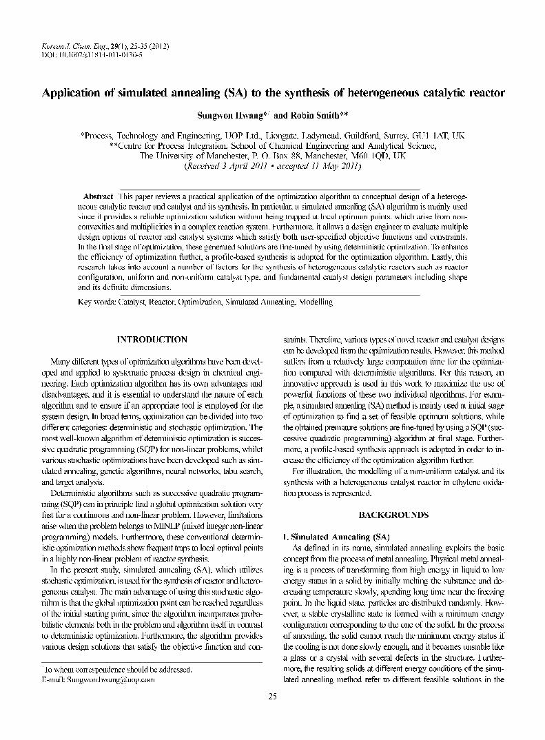
The structure of the simulated annealing algorithm is given in
Fig. 1. The main difference from the precedent algorithm is that
Fig. 1. The structure of the simulated annealing algorithm.

Application of simulated annealing (SA) to the synthesis of heterogeneous catalytic reactor 27
Korean J. Chem. Eng.(Vol. 29, No. 1)
single loop of the local search algorithm is replaced by a double
loop in the SA algorithm. The temperature is changed in the outer
loop, and the number of neighbor moves (Markov chain length) is
changed at each temperature in the inner loop. The key features of
the simulated annealing algorithm are as follows, and they are briefly
explained in the next section.
1. Generation of random changes
2. Markov process
3. Cooling schedule
3. Key Features of Simulated Annealing (SA)
3-1. Generation of Random Changes
Knuth developed a methodology of generating a random num-
ber to produce a new solution of the objective function [7]. This
generator includes random changes and allows all possible solu-
tions to be reached. The new solution can be produced by using
the following equation, based on the random number of v, that lies
between 0 and 1.
y'=ylower+abs(yupper−ylower)×ϖ (1)
Where, y' is a new value of the perturbed variable, ylower/yupper are
lower/upper bounds of the perturbed variable. ϖ is the random num-
ber.
A set of perturbation probabilities is applied to produce the modi-
fication of variables during optimization. For example, higher per-
turbation probabilities induce bigger modification of the variables.
This perturbation probability enables the flexibility of the optimi-
zation. In practice, if the solution in the system is very sensitive to
the optimization variables, higher probabilities must be applied to
the optimization variables.
3-2. Markov Process
The simulated annealing algorithm is based on the theory of
Markov chains that provides the essential background of a Monte
Carlo-based algorithm.
A Markov process {xn} can be represented as a series of sequen-
tial events. The transition of the matrix, representing the probability
of moving from i to j, is independent of its past behavior when its
current state is known. The mathematical form of Markov prop-
erty is formulated as follows [8].
Tij {xn+1=j|xn=i}=Tik j {xn+1=j|x0=i0 …, xn−1=in−1, xn=i} (2)
∀ik, i j∈S, ∀n, k∈N0
Where,
Tij: transition matrix
n: a time point
i, j, ik: states of system
S: state space
Transition probabilities from state i to j are stored in the transi-
tion matrix, Tij, and the sum of the values in each row becomes unity
[9].
If the transition probabilities are constant throughout the events,
it is defined as a homogeneous process, while the variation of the
transition probabilities with time is defined as a heterogeneous pro-
cess. Simulated annealing can be described as a heterogeneous Markov
process because the transition probabilities change with different
annealing temperature. The transition probabilities are a function
of the annealing temperature. Markov chain length is one of the
important variables to be specified at the initial stage. If the chain
length is unnecessarily long, it reaches a global optimum point with
the extra cost of high computation time. On the other hand, too short
a chain length cannot guarantee a global optimum solution. For this
reason, this chain length must be carefully considered at the initial
stage.
According to Dekkers and Aarts, the chain length is decided by
problem dimension as follows [10]:
MCL=10×nd (3)
Where, nd is dimensionality of the problem. Markov chain length
increases with increased dimensionality of the problem. However,
an appropriate selection of this Markov chain length is rather con-
troversial and it should be adjusted by trying various different values
[11]. In this work, various lengths were applied by trial and error in
the range of 6 to 30, depending on the problem, and the most ap-
propriate number was selected for each case.
As shown in Fig. 1, there are two loops, an inner loop and an outer
loop. The inner loop is the Markov process loop and the outer loop
adjusts the annealing temperature. The inner loop is terminated when
the total number of modifications reaches the total Markov chain
length, MCL, or the number of accepted moves reaches MCL/2. The
application of the above statements allows the computation time to
be reduced effectively at high temperature. In a high temperature,
MCL/2 is mostly used for the termination of the loop, because the
acceptance ratio of modifications is much higher than the case of
low temperature. However, longer computation time is needed to
attain the global optimum solution at a low temperature.
Because the SA algorithm does not require derivative informa-
tion, it merely needs to be supplied with an objective function for
each trial and the solution that it generates. Thus, the evaluation of
the problem functions is essentially a ‘black box’ operation in the
perspective of the optimization algorithm. To assess the objective
functions which are produced with new modified variables during
optimization, acceptance criteria should be applied. The acceptance
criteria proposed by Metropolis et al. are used in this work [1]. A
Boltzmann distribution is used to find probability of acceptance, Pij
and an acceptance criterion, Bij is defined as follows.
∆Eij=(Ei+1−Ei) (4)
Pij=exp(−∆Eij/Ta) (5)
Bij(Ta)=min(1, Pij) (6)
∀i≠j, i, j∈S, Ta∈R+
If the change in energy is negative, all new configurations are
accepted. However, if the change in energy is positive, it is accepted
with a probability given by the Boltzmann factor, exp(−∆Eij/Ta).
For example, when the energy change is positive, the high temper-
ature allows higher probabilities in the acceptance criteria. On the
other hand, small value of probability in acceptance criteria is attained
for low temperatures from the above equations. Once new moves
are accepted, the solutions are evaluated again with regard to the
constraints of the problem. By iterating all these procedures, a global
solution that satisfies all design constraints can finally be attained.
3-3. Cooling Schedule
Cooling schedule is one of the most important features of the SA

28 S. Hwang and R. Smith
January, 2012
algorithm. It determines the degree of uphill movement during the
search. In practice, an initial temperature should be high enough to
‘melt’ the system completely and be decreased in some way to the
‘freezing point’. However, selection of the cooling schedule for practi-
cal purposes is still something of a black art [12]. The equation of
cooling schedule, introduced by Aarts and Van Laarhoven, is em-
ployed in this work as follows [13]:
(7)
Where,
σ: Standard deviation of the objective function
Ta
k: Annealing temperature
θ: Cooling parameter
The cooling parameter controls the rate of temperature decrease
during the optimization. The temperature decrease becomes faster
as the annealing parameter takes bigger values. In the meantime,
the probability of being trapped in a local optimum point becomes
higher with a bigger value of the annealing parameter. Typical values
of the annealing parameter are between 0.01 to 1.0. In this work, a
value of 0.05 is employed.
As shown in Fig. 1, the annealing temperature loop is terminated
when the temperature reaches a final temperature or the modifica-
tion is no longer accepted for ‘m×MCL’. The value of ‘m’ should
be selected carefully, depending on the type of optimization prob-
lem. Too small a value allows that optimization is terminated while
it still produces a local optimum solution. On the other hand, too
high value generates unnecessarily long computation time. Mehta
proposed 5 for reactor network synthesis and Choong employed
10 for batch crystallization [14,15]. In this work, a value of 3 is applied
for the optimization of heterogeneous reactor designs.
PROFILE-BASED SYNTHESIS APPROACH
For industrial application of reactor and catalyst modelling and
its synthesis, a number of variables should be considered simulta-
neously, which leads to a significant computational burden for opti-
mization. For example, catalyst type, size, active material distribution
at each stage of the reactor, operating temperature along the reactor
operation period, etc. should be accounted simultaneously for the
maximum performance of the reactor with high selectivity. There-
fore, in some cases, it was found to be much more efficient to op-
timize a profile of the continuous variable which is manipulated by
a set of variables rather than optimizing discrete variables within a
full range boundary. For example, to produce different types of tem-
perature profiles for a certain operation period during optimization,
a mathematical equation must be applied to describe a temperature
profile. This equation can be any type, such as first order, second
order, exponential, asymptotic and so on. Since there are many dif-
ferent types of equations, it is rather inefficient and time consum-
ing to apply every single possible equation in the model. Therefore,
a profile-based synthesis approach has been applied to the work.
Metha and Kokossis applied it to generate optimized temperature
profiles through the axis of a reactor [16]. However, there were some
limitations to describe specific types of profiles. Therefore, Choong
later extended this method to cover a broader range of profiles [15].
In principle, Eqs. (8) and (9) allow various types of profiles to
be generated by combining two different types of profiles, exponen-
tial and asymptotic curves. The first profile in Eq. (8) is an exponen-
tial curve and the second profile in Eq. (9) is an asymptotic curve.
Type I (exponential curve)
(8)
Type II (asymptotic curve)
(9)
Where,
S: pellet location within pellet length
Z: Volumetric activity value
Z1: Inlet value
Z2: Outlet value
To generate every feasible shape of profile, the two curves are
tied together at a certain point and height inside a pellet, for exam-
ple. This tied-in point is controlled by two variables (TB1 and Z3).
Also, the slope of each curve is controlled by variables A1 and A2.
In this case, four to six variables are manipulated to generate various
profiles with fixed initial and final points. The type of profile is de-
termined by the variables A1, A2, TB1, Z1, Z2 and Z3.
A1: The power of equation type II (A1≥1)
A2: The power of equation type I (A2≥1)
Z3: The volumetric activity value corresponding to TB1 (value be-
tween 0 and 1/3 for sphere, 1/2 for cylinder and 1 for slab)
TB1: Intermediate peak point for the curve (−1<TB1<0 for Type I+
Type II, 0<TB1<1 for Type II+Type I)
The application is applied to case studies which will be described
in Section 5.
MODELLING OF HETEROGENEOUS CATALYTIC
REACTOR
1. Heterogeneous Catalytic Reactor
Heterogeneous catalytic reactors have been workhorses in the
large-scale chemical product industry. Fixed-bed reactors have been
preferred because of relatively low cost and simplicity of applica-
tion compared with fluidized-bed or moving bed reactors. Fixed-
bed reactors have been increasingly used in recent years, especially
in gas-phase reactions. They can be categorized into several differ-
ent configurations according to applications, as follows [17].
• Single adiabatic reactor: exothermic or endothermic non-equi-
librium limited reaction (e.g., mild hydrogenation process).
• Adiabatic bed reactors in series with intermediate heat exchange:
high conversion, equilibrium-limited reactions (e.g., SO2 oxidation, cat-
alytic reforming, ammonia synthesis and hydro-cracking processes).
• Multi-tubular non-adiabatic reactors: highly endothermic or
exothermic reactions requiring close temperature control to obtain
high selectivity (e.g., hydrogenation and oxidation process).
• Direct-fired non-adiabatic reactors: highly endothermic reac-
tions with high temperatures (e.g. steam reforming process).
Mass and energy balances used for the design of the heteroge-
neous catalytic reactor are described below.
Ta
k+1= Ta
k
1+
1+ θ( )Ta
k
ln
3σ Ta
k( )-------------------------
⎝ ⎠⎛ ⎞
−1
Z s( ) = Z1− Z1− Z2( ) s
stotal
--------⎝ ⎠⎛ ⎞
A2
Z s( ) = Z2 − Z2 − Z1( )stotal − s
stotal
---------------⎝ ⎠⎛ ⎞
A1

Application of simulated annealing (SA) to the synthesis of heterogeneous catalytic reactor 29
Korean J. Chem. Eng.(Vol. 29, No. 1)
For the Bulk/Fluid Phase:
The fluid phase mass and energy balances for heterogeneous,
non-isothermal, non-adiabatic plug flow reactors are shown below.
- Mass balance
(10)
- Energy balance
(11)
- Boundary condition,
(12)
Where, ν=velocity of external fluid phase
Where, Cf, i=fluid concentration on species in bulk phase, I
Where, Z=axial co-ordinate along the reactor
Where, ε=bed void fraction
Where, νi, j=stoichiometric coefficient of species, i in reaction j
Where, rj=rate of reaction, j
Where, ρ=density of fluid phase
Where, Cp=heat capacity of fluid phase
Where, ν =velocity of external fluid phase
Where, Tf =temperature of fluid phase
Where, ∆Hj=heat of reaction j
Where, Uo=overall heat transfer coefficient between reaction gases
and cooling medium
Where, α=4/Dt (internal tube diameter)
For the Fluid/Particle Interface:
The mass and energy balances in catalyst phase with external
transfer resistances are shown below.
- Mass balance
(13)
- Energy balance
(14)
Where, kg, i=external mass transfer coefficient of component I
Where, Cs, i=fluid concentration on species on the surface of the
catalyst, I
Where, De, i=effective diffusivity coefficient of component, I
Where, x=distance from pellet centre to surface
Where, η=effectiveness factor
Where, rs, j=rate of reaction, j on catalyst surface
Where, ρp=density of pellet
Where, S'=characteristic pellet length (=Vp/Sp)
Where, Vp=volume of pellet
Where, Sp=surface of pellet
Where, h=external heat transfer coefficient
Where, Ts=temperature of catalyst surface
Where, Tf =temperature of fluid phase
Where, λ=effective thermal conductivity
For the Catalyst Particle:
The mass and energy balances in catalyst phase with internal dif-
fusional resistances are shown below.
- Mass balance
(15)
- Energy balance
(16)
- Boundary condition
Where,
x=1; Ci=Cs, i, T=Ts
n=integer characteristic of pellet geometry
n=0 for infinite slab; n=1 for infinite cylinder; n=2 for sphere
a(x)=1 for uniform catalyst
Ci=concentration of component I
a(x)=activity distribution function
In this work, a plug-flow packed-bed reactor is regarded as a num-
ber of sub-PFRs in series. To increase computational efficiency of
the optimization problem, effectiveness factor is obtained at the inlet
of each sub-PFR and applied to the sub-PFR’s. In the meantime,
the accuracy of the heterogeneous catalytic reactor model and com-
putational requirements for optimization are controlled by manipu-
lating the number of sub-PFRs. This method allows producing more
νdCf i,
dz---------- = − 1− ε( ) υi j, rj⋅( )∑⋅
ρcpνdTf
dz------- = 1− ε( ) − ∆Hj rj⋅( ) − Uoα Tf − Tc( )∑
z = 0: Tf = Tf
o, Cf i, = Cf i,
o
kg i, Cs i, − Cf i,( ) = − De i,
dCi
dx-------- = η υi j, rs j,⋅( )ρpS'∑
h Ts − Tf( ) = − λdT
dx------ = η ∆Hj rs j,⋅( )ρpS'∑
De i,
1
xn
----d
dx------ x
ndCi
dx--------
⎝ ⎠⎛ ⎞
= υi j, rj⋅( ) a x( )⋅∑
λ1
xn
----d
dx------ x
ndT
dx------
⎝ ⎠⎛ ⎞
= − − ∆Hj( ) rj⋅[ ] a x( )⋅∑
x = 0; dCi
dx-------- =
dT
dx------ = 0
Fig. 2. Schematic non-isothermal and non-adiabatic reactor design with different catalyst dilution in two bed zones.
30 S. Hwang and R. Smith
January, 2012
accurate results of the model within a reasonable optimization time.
The equations above are applied to the mass and energy balances
of the fluid phase, internal and external catalyst phases [18-20]. A
reactor is divided into several bed zones which are arranged with
different types of catalysts, and a set of sub-PFRs represents a bed
zone inside a reactor. By using this method, various reactor designs
can be considered. For example, any number of reactor beds can
be specified and different degrees of catalyst dilution can be applied
to each bed, as described in Fig. 2. For the modelling of a multi-
tubular reactor, the number of tubes, the length and diameter of each
tube must be specified in order to calculate heat exchange area, which
plays a critical role in non-isothermal reactions. Furthermore, inlet
coolant temperature, reactor volume, injection type of coolant, heat
transfer coefficient, etc. should be applied in reactor modelling.
Pellet Size and Shape:
Pellet size must be considered at the reactor design stage. As shown
in Eqs. (17) and (18), the pellet size is closely related to the Thiele
modulus and the effectiveness factor. For example, this correlation
can be deduced from Eq. (15) in a dimensionless form [18].
(17)
Where, ϕ2 is the Thiele modulus:
(18)
Where, y' is concentration fraction, ρp is density of pellet, νij is
stoichiometric coefficient of species, i in reaction j and De, i is effec-
tive diffusivity of component i.
The pellet size is also optimized along the reactor axis to control
the activities of the different catalyst beds. In general, a high activity
can be obtained from a small pellet, while activity drops as the cata-
lyst dimension increases due to high diffusional resistances inside a
pellet. However, if the pellet becomes too small, the pressure drop
may increase beyond the allowable pressure drop of the reactor.
Therefore, the pressure drop must be carefully monitored as the pellet
dimensions vary.
To consider various shapes of pellets for the calculation of the
effectiveness factor, characteristic pellet shape and dimension param-
eters were developed by Aris [21]. This characteristic pellet dimension
number is calculated as a ratio of pellet volume to surface area, and
pellet shape number ranges between 0 (infinite slab) and 2 (sphere).
However, this allows only one pellet dimension to characterize the
pellet shape, while the pellet length of the catalyst is assumed to be
infinite. For this reason, the method applies only to spherical type
of catalyst, providing results with reasonable accuracy since this is
the only shape that has one pellet dimension. To compensate for
the weakness, Burghardt and Kubaczka developed a new method
[22]. For example, a new characteristic pellet shape and dimension
numbers were developed based on three dimensions of the pellet
in order to consider the impact of geometrical pellet shape on its
activity. These new characteristic pellet shape and dimension num-
bers are employed to this work to obtain more accurate catalyst ef-
fectiveness factors. The detailed calculation procedure can be found
in the paper of Burghardt and Kubaczka [22].
Effectiveness Factor:
The catalyst performance can be defined by an effectiveness factor
and described by the following equation [23].
(19)
Where, η is effectiveness factor, fj is dimensionless reaction rate
j, a is activity distribution function and s is dimensionless catalyst
phase co-ordinate.
Eqs. (10)-(16), with Cf, i, Tf solved from the differential equa-
tions along the reactor axis, the unknown variables Cs, i, Ts in each
section of the plug-flow reactor and the Ci, T profile within the pellet,
were solved continuously using a non-linear equation solver. Eqs.
(15) and (16) were solved as a two point boundary-value problem
using a Runge-Kutta-Merson method and a solver in a shooting
and matching technique (NAG Fortran Library, D02HAF).
The heterogeneous reactor model offers higher accuracy for the
design of the reactor. On the other hand, it suffers from the lack of
catalyst related data including heat transfer and diffusional resis-
tances. It is also computationally more demanding than a pseudo-
homogeneous model. Therefore, the pseudo-homogeneous model
is more applicable for conceptual reactor design in the early stage,
whereas a heterogeneous model is followed for rigorous analysis.
Mixing Rule of Inert Catalyst:
The inert fraction at reactor bed is defined as follows:
(20)
Inert fraction is multiplied to the bulk density of pure catalyst
mixture in each bed and used for the mass and energy balance equa-
tions through the reactor axis [24-26].
For the modelling of the catalyst bed, an assumption of even fluid
distribution across the bed is used [27]. For example, perfect homo-
geneous mixing of both the inert particles and the catalyst particles
is not possible due to their finite dimensions and changes in resi-
dence time distribution occur. These effects decrease with increas-
ing ratio of bed length to particle diameter. However, this behavior
is not considered in this work.
Superstructure of Reactor Model:
For the design of feed stream distribution, mass and heat bal-
ance of the side and main streams inside a reactor should be con-
sidered. As described in Fig. 3, the reactor model comprises a num-
ber of sub-PFRs. Each sub-PFR should be allowed to be con-
nected with a side-stream in a superstructure, satisfying the mass
and energy balance during optimization. The superstructure of all
stream connections between side and main streams is built by using
a flag function. The general procedure for simulation and optimi-
zation of reactor design is illustrated in Fig. 3.
This method enhances conceptual reactor design by considering a
number of various configurations of side or main streams and cata-
lyst dilution during optimization. A penalty function is used to optimi-
zation algorithm in order to keep the temperature profile of reactor
within allowable range along the reactor axis during optimization.
1-1. Non-uniform Catalyst
Many researchers have demonstrated that various types of non-
uniform activity distribution profiles can be generated by using im-
pregnation techniques. Maatman illustrated the use of co-impreg-
nation as a means of controlling the active catalyst material distri-
d2
y'
ds2
--------- = − n
s---
dy'
ds------- + ϕ
2
ρp − υi j, fj⋅( )∑
ϕ2
= Rs j, Rp
2
De i, Cs i,
---------------
ηj =
fja s( )snds
0
1
∫
a s( )snds
0
1
∫--------------------------
α' = Vdiluted
Vdiluted + Vundiluted
-----------------------------------

Application of simulated annealing (SA) to the synthesis of heterogeneous catalytic reactor 31
Korean J. Chem. Eng.(Vol. 29, No. 1)
bution in a pellet for the case of platinum deposition from chloroplatinic
acid on alumina support [28]. Since then, co-impregnation tech-
niques have been widely used to prepare non-uniformly distributed
catalysts. Shyr and Ernst showed that numerous types of non-uni-
form catalyst pellet profiles could be prepared by using impregnation
techniques [29]. In their works, different types of chemical additives
(co-ingredients), chemical additive concentration and impregnation
time were controlled to produce various non-uniform Pt activity
distribution profiles in spherical γ-alumina beads. Their research
used HCl, HF, HNO3, acetic acid, citric acid, tartaric, AlCl3, NaCl,
NaF, NaBr, NaNO3, Na3PO4, Na benzoate, and Na citrate. Two dif-
ferent impregnation times were used (1 hour and 22 hours). The
results showed nine different types of pellets as a result, as described
in Fig. 4.
These experiments demonstrate that various types of active ma-
terial distribution profile can be manufactured once a specific type
of optimal profile has been designed. Furthermore, the location of
active material distribution inside a pellet changes according to the
impregnation time.
1-2. Modelling Of Non-uniform Catalyst
To describe the non-uniform distribution inside a catalyst pellet,
the activity distribution factor is introduced. The a(x) in Eqs. (15)
and (16) must satisfy the normalization condition [30].
(21)
The above equations can be converted into a dimensionless form
by introducing the variables:
Where, Vp is volume of pellet p, a is activity distribution func-
tion, s is dimensionless catalyst phase co-ordinate, x is distance from
pellet center to surface, Rp is radius of pellet and r is rate of reaction,
j.
Furthermore, Eq. (21) can be expressed in a general form:
(22)
Where, n is integer characteristic of pellet geometry, number of
sub-PFR (n=0 for infinite slab; n=1 for infinite cylinder; n=2 for
sphere).
By combining the above equations with Eq. (19), the effective-
1
Vp
------ a x( )dVp =1V
p
∫
s = x
Rp
-----, fj = rj
rs j,
-----
a s( )snds =
1
n +1----------
0
1
∫
Fig. 3. The algorithm for reactor design simulation and optimiza-tion.
Fig. 4. Types of Pt profiles obtained by co-impregnation (repro-duced from Journal of Catalysis, 1980, 63, 425).

32 S. Hwang and R. Smith
January, 2012
ness factor of non-uniform activity distribution profile inside a pellet
is produced, and it is applied to energy and mass balance equations
at each sub-PFR.
The integration of activity profiles through the pellet volume at
certain type of pellet, such as slab, cylinder and sphere can be carried
out by using Eq. (22). Since inlet and outlet values of each shape
of catalyst are fixed, only the shape of the integrated activity profile
can be changed during optimization between two fixed values. After
a certain type of profile has been generated, the corresponding profile
is transformed to an activity distribution profile through the pellet.
Lastly, the concentration profiles of all components inside a pellet
are generated based on the second-order boundary value problem,
and they are used to generate an appropriate effectiveness factor.
Typical volumetric activity profiles of spherical catalyst involving
egg-yolk, egg-shell and middle peak type are shown in Fig. 6.
For an optimization of activity distribution profile, various volu-
Fig. 5. Activity distribution profile examples for non-uniform catalyst.
Fig. 6. Example of reactor design configurations: (a) Five-bed reactor with optimum inert catalyst mixing, (b) Three-bed and multi-tubularreactor with optimum inert catalyst mixing and ethylene side stream, (c) Packed-bed membrane reactor, (d) Five-bed multi-tubularreactor configuration with inert and surface layered catalyst mixing.

Application of simulated annealing (SA) to the synthesis of heterogeneous catalytic reactor 33
Korean J. Chem. Eng.(Vol. 29, No. 1)
metric activity profiles for a spherical type of pellet and the corre-
sponding activity distribution profile inside a pellet are generated
through a profile-based synthesis approach.
Typical non-uniform catalysts are briefly summarized in Fig. 5.
Further detailed discussion about mathematical modelling of each
type of non-uniform catalyst is illustrated by Hwang [31].
APPLICATION
1. Ethylene Oxidation Process
Ethylene oxide is produced by vapor-phase oxidation of ethyl-
ene with oxygen or air on a supported silver catalyst. In general,
the composition of the feed stream contains 5 to 10 vol% ethylene
and 5 to 10 vol% oxygen as reactants, and nitrogen is typically used
as an inert gas. Organic coolant is generally used as a cooling me-
dium. The optimum temperature inside a reactor is generally around
230 oC and the selectivity ranges between 70 to 80 percent when
pure oxygen is used instead of air [32].
The reaction kinetics is obtained from the work of Klugherz and
Harriott [33]. These have previously been employed for the study
of Dirac-delta catalysts by Morbidelli et al. and Baratti et al. [18,
34]. The effective diffusivity coefficients are obtained from Satter-
field, and thermal conductivity of alumina pellets are obtained from
Mischke and Smith [32,35]. External heat and mass transfer coeffi-
cients are obtained from the data of Baratti et al. [18].
Reaction 1
∆H=−120,036 kJ/kmol (23)
Reaction 2
∆H=−1,324,280 kJ/kmol (24)
The above reaction is a typical industrial ethylene oxidation pro-
cess, and the related computational data are given in Table 1.
Reactor design data is taken from the reports of ethylene oxide
revamping projects by Coombs et al. and Huang et al. [36,37]. The
data are as follows:
Reactor size
• Tube diameter=0.03912 m
• Tube length=12.8 m
• Tube material=Carbon steel
• Number of tubes=2781
• Total heat transfer area=4396 m2
• Overall heat transfer coefficient=0.176 kW/m2 K
• Total reactor volume=43 m3
• Catalyst density=881 kg/m3
• Catalyst per reactor=9,431 kg
Feed molar flow (kmol/hr)
• Ethylene=100
• Nitrogen=1075
• Carbon dioxide/ Ethylene oxide/ Water=0
• Oxygen=75
In general, bigger size of pellet and inner location of active material
C2H4 +
1
2---O2 C2H4O→
C2H4 + 3O2 2CO2 + 2H2O→
r1= k1c1c2
2
/F1
2
r2 = k2c1c2
2
/F2
2
F1= 0.0106 + 2144c1+ 805c2( ) 1+1271 c2( )⋅
F2 = 0.008 + 4166c1+1578c2( ) 1+ 718 c2( )⋅
k1= k1
0
γ1 θ −1( )/θ[ ]exp
k2 = k2
0
γ2 θ −1( )/θ[ ]exp
Table 1. Computational parameters for the ethylene oxide process
k1o=8.63×10⁶ mol/s cm3 Rp=0.25 cm, n=2
k2o=6.57×10⁶ mol/s cm3 Silver catalyst
De, 1=0.003 cm2/s xof, 1=0.08, xo
f, 2=0.06, xof, 3=0.86
De, 2=0.004 cm2/s kg, 1=4.5 cm/s, kg, 2=5.44 cm/s
γ1=21.9, γ2=29.7 λ=2.2e−4 kW/m·K, h=0.88 kW/m2·K
Table 2. Summary of various reactor designs in ethylene oxida-tion
Case 1 Case 2 Case 3 Case 4
Yield (%) 39.2 45.7 45.4 032.4
Yield increase (%) - 16.6 15.8 −17.3
Selectivity (%) 74.7 71.7 71.0 074.0
Ethylene oxide product (kmol/hr) 31.5 36.8 36.5 035.9
Maximum temperature (oC) 224 231 234 225
Case 5 Case 6 Case7 Case 8
Yield (%) 42.0 45.5 44.6 045.5
Yield increase (%) 07.2 16.1 13.8 016.1
Selectivity (%) 74.1 73.2 72.7 072.2
Ethylene oxide product (kmol/hr) 33.8 36.6 35.9 036.6
Maximum temperature (oC) 226 229 228 230
Case 9 Case 10 Case 11
Yield (%) 45.0 48.0 46.6
Yield increase (%) 14.8 22.4 18.9
Selectivity (%) 72.8 71.7 71.4
Ethylene oxide product (kmol/hr) 36.2 38.6 37.5
Maximum temperature (oC) 228 231 237
Case 1: Base case
Case 2: Five-bed tubular reactor with optimum inert catalyst mixing
Case 3: Three-bed and multi-tubular reactor with optimum inert cat-
alyst mixing and ethylene side stream
Case 4: Packed-bed membrane reactor
Case 5: One-bed reactor with surface layered catalyst (10% thick-
ness)
Case 6: Three-bed reactor with optimum active material location inside
Dirac-d catalyst
Case 7: Three-bed reactor with optimum active material location inside
layered catalyst (10% thickness)
Case 8: Three-bed reactor with optimum active material location obtained
from profile based synthesis (PBS)
Case 9: Three-bed reactor with optimum pellet size with surface lay-
ered catalyst (10% thickness)
Case 10: Five-bed tubular reactor under optimum inert catalyst mix-
ing with pure surface layered catalyst (10% thickness)
Case 11: Three-bed and multi-tubular reactor under optimum inert
catalyst mixing with pure surface layered catalyst (10% thickness)
and oxygen sidestream

34 S. Hwang and R. Smith
January, 2012
generate low activity. However, this characteristic can be benefi-
cially applied for the control of temperature inside a reactor. The
heat gradient inside a pellet adds complexity to predict the activity
at certain conditions, since the reaction rate is very sensitive to local
temperature inside a pellet. Furthermore, in a particular case of the
ethylene oxidation reaction, it was found that the use of small size
of catalyst pellet or active material distribution near the catalyst sur-
face produced higher selectivity at the same operating conditions.
Under these complex conditions, various reactor and catalyst param-
eters below were optimized in a multi-bed tubular reactor.
1. Non-uniform catalyst
a. Surface layered catalyst
b. Dirac-delta catalyst
c. General non-uniform catalyst (egg-yolk, egg-shell, middle-peak,
etc.)
d. Layered catalyst
2. Number of reactor beds
3. Pellet dimension
4. Reactor configuration (side stream distribution, inert catalyst mix-
ing, membrane reactor)
For the optimization of reactor and catalyst synthesis, simulated
annealing is initially applied to produce a set of reasonable solu-
tions and each solution is further optimized by using a determinis-
tic algorithm.
Table 2 shows the summary of the optimization results based on
different combinations of the above variables for the synthesis of
heterogeneous catalytic reactor, and some examples of feasible reac-
tor designs are shown in Fig. 6.
In this work, 70% of minimum selectivity was used as a con-
straint for the maximization of yield. In total, 11 different types of
reactor configurations are produced after optimization. For exam-
ple, the maximum yield of 48%, which shows 22.4% increase, is
achieved by using a combination of inert catalyst mixed with sur-
face layered catalyst in a five-bed tubular reactor.
Furthermore, it was observed during the analysis of optimiza-
tion results that selectivity decrease could be minimized by using a
thin layered active material distribution on the catalyst surface rather
than uniform active material distribution particularly in ethylene oxi-
dation process.
CONCLUSION
Optimum synthesis of a heterogeneous catalytic reactor has been
achieved through the combination of simulated annealing and deter-
ministic optimization. It was observed that the application of simu-
lated annealing is more effective for the design of reactor and catalyst,
and its synthesis because of its capability to provide a set of good
solutions which meet an objective function in a fixed amount of
time rather than one best possible solution. Therefore, this method
can be used as a targeting tool as well as an analysis tool so that a
design engineer can evaluate several feasible system designs as an
alternative option. Furthermore, the stochastic algorithm has been
proven to be much more powerful in avoiding any trap from local
optima.
Clearly, long computational time has been a significant draw-
back for a simulated annealing process. Therefore, a deterministic
optimization is applied at the late stage of optimization to avoid un-
necessary delay in reaching a final optimum solution. Furthermore,
profile-based synthesis is adopted to reduce complexity burden. In
this study, manipulation of only a few set of variables allowed genera-
tion of various types of different profiles, and it was proved that
this methodology greatly enhanced the efficiency of optimization.
Synthesis of heterogeneous catalytic reactors has been reviewed
with industrial application by covering the following items.
- Novel configuration of reactor system (side stream distribu-
tion, inert catalyst mixing, membrane reactor, etc.)
- Modelling of catalyst with infinite dimension and its shape.
- Non-uniform catalyst (Dirac-delta, profile synthesis, layer type)
- Catalyst deactivation
For industrial application, the ethylene oxidation process is illus-
trated with the optimization results, showing a variety of feasible
design alternatives to a design engineer. Furthermore, the optimiza-
tion results proved significant increase of yield and selectivity in
ethylene oxidation process.
NOMENCLATURE
A1 : the power of equation type II
A2 : the power of equation type I
a(x) : activity distribution function
ad, j : catalyst deactivation function
Bij : acceptance probability from the state (i) to (j)
Ci : concentration of component i
Cp : heat capacity of fluid phase
Cf, i : fluid concentration on species in bulk phase, i
Cs, i : fluid concentration on species on the surface of the catalyst, i
De, i : effective diffusivity coefficient of component, i
Ei, f : objective function
h : external heat transfer coefficient
kg, i : external mass transfer coefficient of component i
MCL : Markov chain length
nd : dimensionality of the problem
Pij : acceptance probability from state (i) to (j)
rj : rate of reaction, j
rs, j : rate of reaction, j on catalyst surface
Rp : radius of pellet
S : state space
s : dimensionless catalyst phase co-ordinate
S' : characteristic pellet length (=Vp/Sp)
T, Ta : annealing temperature, local temperature inside a pellet
t : reactor operation time or catalyst cycle period
Tao : initial annealing temperature
TB1 : intermediate peak point for the curve
Tc : temperature of surrounding coolant
Tf : final annealing temperature, temperature of fluid phase
Ts : temperature of catalyst surface
Tij : transition matrix
Uo : overall heat transfer coefficient between reaction gases and
cooling medium
V : volume
Vp : volume of pellet
x : control variable, distance from pellet centre to surface
y' : new value of the perturbed variable
ylower : lower bound of the perturbed variable

Application of simulated annealing (SA) to the synthesis of heterogeneous catalytic reactor 35
Korean J. Chem. Eng.(Vol. 29, No. 1)
yupper : lower bound of the perturbed variable
Z : axial co-ordinate along the reactor, volumetric activity value
Z1 : inlet volumetric activity value
Z2 : outlet volumetric activity value
Z3 : the volumetric activity value corresponding to TB1
Subscripts
i, j, k : states of system
n : time point, integer characteristic of pellet geometry (n=0
for infinite slab; n=1 for infinite cylinder; n=2 for sphere)
Superscripts
c : coolant
f : fluid phase
i : component
j : reaction
p : pellet
o : initial condition
s : catalyst surface
Greek Letters
α : 4/Dt
α' : inert volume fraction
∆H : heat of reaction
δ : deviation of two objective functions located at different states
ε : bed void fraction
η : effectiveness factor
ϕ : Thiele Modulus ( )
λ : effective thermal conductivity
ν : velocity of external fluid phase
νi, j : stoichiometric coefficient of species, i in reaction j
θ : cooling control parameter
ρ : density of fluid phase
ρp : density of pellet
σ : standard deviation of the objective function
ϖ : random number
REFERENCES
1. N. Metropolis, A. W. Rosenbluth, M. N. Rosenbluth, A. H. Teller
and E. Teller, J. Chem. Phys., 21(6), 1087 (1953).
2. M. Pincus, Oper. Res., 18, 1225 (1970).
3. S. Kirkpatrick, C. D. Gelatt and Jr. M. P. Vecchi, Science, 220, 671
(1983).
4. R. W. Eglese, European J. Operational Research, 46, 271 (1990).
5. F. Glover and H. J. Greenberg, European J. Operational Research,
39, 119 (1989).
6. P. J. M. Van Laarhoven and E. H. L. Aarts, Simulated Annealing:
Theory and Applications, Reidel, Dordrecht (1987).
7. D. E. Knuth, The art of computer programming, Vol. II (2nd Ed.),
Addison-Wesley, London (1981).
8. H. M. Taylor and S. Karlin, An introduction to stochastic modelling
(3rd Ed.), Academic Press, London (1998).
9. M. Iosifescu, Wiley Series in Probability and Mathematical Statis-
tics: Finite Markov process and their applications, John Wiley and
Sons Ltd. (1980).
10. A. Dekkers and E. Aarts, Mathematical Programming, 50(3), 367
(1991).
11. E. C. Marcoulaki, Ph.D. Thesis, UMIST, UK (1998).
12. D. G. Bounds, Nature, 329, 215 (1987).
13. E. H. L. Aarts and P. G. M. Van Laarhoven, Philips J. Res., 40(4),
193 (1985).
14. V. L. Mehta, Ph.D. Thesis, UMIST, UK (1998).
15. K. L. Choong, Ph.D. Thesis, UMIST, UK (2002).
16. V. L. Metha and A. Kokossis, Com. Chem. Eng., 21(S1), S325
(1997).
17. H. F. Rase, Fixed-bed reactor design and diagnostics, Butterworths
(1990).
18. R. Baratti, A. Gavriilidis, M. Morbidelli and A. Varma, Chem. Eng.
Sci., 49(12), 1925 (1994).
19. M. M. J. Quina and R. M. Ferreira, Ind. Eng. Chem. Res., 38, 4615
(1999).
20. M. M. J. Quina and R. M. Ferreira, Chem. Eng. Sci., 55, 3885 (2000).
21. R. Aris, Chem. Eng. Sci., 6(6), 262 (1957).
22. A. Burghardt and A. Kubaczka, Chem. Eng. Proc., 35, 65 (1996).
23. M. Morbidelli, A. Gavriilidis and A. Varma, Reactors, and mem-
branes, Cambridge University Press (2001).
24. M. M. J. Quina and R. M. Ferreira, Ind. Eng. Chem. Res., 38, 4615
(1999).
25. M. M. J. Quina and R. M. Ferreira, Chem. Eng. J., 75, 149 (1999).
26. M. M. J. Quina and R. M. Ferreira, Chem. Eng. Sci., 55, 3885 (2000).
27. C. M. Van Den Bleek, K. Van Der Wiele and P. J. Van Den Berg,
Chem. Eng. Sci., 24, 681 (1969).
28. R. W. Maatman, Ind. Eng. Chem., 51(8), 913 (1959).
29. Y. Shyr and W. R. Ernst, J. Catal., 63, 425 (1980).
30. Y. C. Yortsos and T. T. Tsotsis, Chem. Eng. Sci., 37(9), 1436 (1982).
31. S. Hwang, Ph.D. Thesis, UMIST, UK (2003).
32. C. N. Satterfield, Chemical Engineering Series, Heterogeneous Catal-
ysis in Practice, McGraw-Hill (1980).
33. P. D. Klugherz and P. Harriott, AIChE J., 17, 856 (1971).
34. M. Morbidelli, A. Servida, R. Paludetto and S. Carra, J. Catal., 87,
116 (1984).
35. R. A. Mischke and J. M. Smith, Ind. Eng. Chem. Fundam., 1, 288
(1962).
36. J. Coombs, D. Kim and L. Palombo, Report of ethylene oxide reac-
tor revamp, Department of Chemical Engineering, Rice University
(1997).
http://www.owlnet.rice.edu/~ceng403/ethox97.html
37. J. Huang, D. Resendez and G. Tran, Ethylene Oxide Reactor Sys-
tem, Department of Chemical Engineering, Rice University, (1999).
http://www.owlnet.rice.edu/~ceng403/gr1599/finalreport3.html
= Rp
rs j,
De i, Ci
------------
![REFERENCI: 2612013 I D.] 1AT 2013 PtR/ZA/1’O: Z.Besim ... · Banci Republike Kosova; 9. Finansijski sliñbenici-podrazumeva i ukljuëuje Glavnog Administiativnog S1ubenikaSefa finansij](https://static.documents.pub/doc/80x56/5c7b845b09d3f26c268c2238/referenci-2612013-i-d-1at-2013-ptrza1o-zbesim-banci-republike.jpg)


