EUR 23936 EN - 2009

Application of the LOICZ Methodology to the Mediterranean Sea

Robert O. Strobl, José-Manuel Zaldívar Comenges, Francesca Somma, Adolf Stips and Elisa García Gorriz

2

The mission of the JRC-IES is to provide scientific-technical support to the European Union’s policies for the protection and sustainable development of the European and global environment. European Commission Joint Research Centre Institute for Environment and Sustainability Contact information Address: Via E. Fermi 1, TP 272 E-mail: robert.strobl@jrc.ec.europa.eu Tel.: +39 0332789391 Fax: +39 0332785807 http://ies.jrc.ec.europa.eu/ http://www.jrc.ec.europa.eu/ Legal Notice Neither the European Commission nor any person acting on behalf of the Commission is responsible for the use which might be made of this publication.

Europe Direct is a service to help you find answers

to your questions about the European Union

Freephone number (*):

00 800 6 7 8 9 10 11

(*) Certain mobile telephone operators do not allow access to 00 800 numbers or these calls may be billed.

A great deal of additional information on the European Union is available on the Internet. It can be accessed through the Europa server http://europa.eu/ JRC 52454 EUR 23936 EN ISBN 978-92-79-12794-6 ISSN 1018-5593 DOI 10.2788/23549 Luxembourg: Office for Official Publications of the European Communities © European Communities, 2009 Reproduction is authorised provided the source is acknowledged Printed in Italy

3

Table of Contents

1. LOICZ METHODOLOGY 5

1.1 Water budget 7

1.2 Budgets of conservative materials: Salt budgets 8

1.3 Budgets of nonconservative materials 10

2. THE MEDITERRANEAN SEA BASIN 15

2.1 Study Area 15

2.2 Data Provision 18

3. LOICZ BUDGET OF THE MEDITERRANEAN SEA 24

3.1 Water Budget 24

3.2 Salt Budget 27

3.3 DIP Balance 28

3.4 DIN Balance 31

3.5 Stoichiometrically Linking the Nonconservative Budgets 32

4. DISCUSSION AND CONCLUSIONS 33

5. REFERENCES 36

4

List of Tables Table 1. Summary of data used for the LOICZ budget of the Mediterranean Sea. 19 Table 2. Water budget for the Mediterranean Sea. 26 Table 3. Overall flow exchange as computed from Pickard and Emery (1990) and Bryden et al. (1994) as well as from Equation 7. 26 Table 4. Salt budget for the Mediterranean Sea. 28 Table 5. ∆DIP and ∆DIN budgets for the Mediterranean Sea for the time period 1996 to 2005. 30 Table 6. Trend analysis for ∆DIP for the time span of 1996 to 2005. 35 Table 7. Trend analysis for ∆DIN for the time span of 1996 to 2005. 35

List of Figures

Figure 1. Water budget for a coastal water body of volume V1 (Gordon et al., 1996). 8 Figure 2. The salt budget for a coastal water body (Gordon et al., 1996). 9 Figure 3. The budget for a non-conservative material, Y, in a coastal water body (Gordon et al., 1996). 11 Figure 4. Topography of the Mediterranean Sea. The 1000 m contour is shown, and regions deeper than 3000 m are shaded. The 200 m contour is shown as a broken line where it departs significantly from the 1000 m contour. In addition, the 2000 m contour is shown as a broken line in the Black Sea (adopted from Tomczak and Godfrey (2003)). 15 Figure 7. Semi-schematic of the system under consideration for the budget (where ATL = Atlantic Ocean; MED = Mediterranean Sea; BLACK = Black Sea; FR1a = incoming flow from ATL to MED; FR1b = outgoing flow from MED to ATL; FR2a = outgoing flow from MED to BLACK; FR2b = incoming flow from BLACK to MED). 25 Figure 8. Estimated streamflow, precipitation and evaporation for the Mediterranean Sea. 25 Figure 9. Calculated annual amount of dissolved phosphorous and dissolved nitrogen (in kg) discharged to the Mediterranean Sea from its catchments. 30 Figure 10. Estimated ∆DIP and ∆DIN for the time period 1996 to 2005. 31 Figure 11. NEM balance and nfix-dnit variation for the Mediterranean Sea (1996-2005). 32

5

1. LOICZ METHODOLOGY

The coastal zone is an integral part of the catchment-ocean system and is subject to internal and

external forcing from both natural and anthropogenic pressures. The Land-Ocean Interactions in the

Coastal Zone (LOICZ) approach attempts to evaluate coastal change from a system perspective and

assumes that the effects taking place are due to pressures within the whole basin. It assesses the

physical, biogeochemical and human interactions influencing coastal change. The priority focus is

on the transport of water and sediments as well as the cycling of nitrogen, phosphorus and carbon.

Pernetta and Milliman (1995) have summarized the key objectives of the LOICZ approach as

follows:

• to gain a better understanding of the cycles of the key nutrient elements carbon (C), nitrogen (N)

and phosphorus (P) on a local and ultimately on a global scale;

• to understand how the coastal zone affects material fluxes via biogeochemical processes; and

• to characterize the relationship of these fluxes to environmental change, including human

intervention.

More specifically the goals of the LOICZ budget approach are stated in the Science Plan (Holligan

and de Boois, 1993) and Implementation Plan (Pernetta and Milliman, 1995),

•To determine at global and regional scales:

(1) the fluxes of materials between land, sea and atmosphere through the coastal zone

(2) the capacity of coastal systems to transform and store particulate and dissolved matter

(3) the effects of changes in external forcing conditions on the structure and functioning of

coastal ecosystems.

•To determine how changes in land use, climate, sea level and human activities alter the fluxes and

retention of particulate matter in the coastal zone, and affect coastal morphodynamics.

•To determine how changes in coastal systems, including responses to varying terrestrial and

oceanic inputs of organic matter and nutrients, will affect the global carbon cycle and the trace gas

composition of the atmosphere.

•To assess how responses of coastal systems to global change will affect the habitation and usage

by humans of coastal environments, and to develop further the scientific and socio-economic bases

for the integrated management of the coastal environment.

6

The LOICZ methodology not only has the purpose of studying the impact of climatic change and

human activities on fluxes of nutrients to coastal ecosystems, but also of addressing the increasing

need of policy-oriented scientific information. Information on the impact of watershed processes on

nearshore coastal environments is becoming increasingly important for the protection of

biodiversity and sustainability of terrestrial aquatic ecosystems as well coastal systems under their

influence. Such integrated systems require an approach that closely links science and policy for a

more efficient development and implementation of EU Directives.

For constructing biogeochemical budgets for coastal waters LOICZ has developed a set of

Guidelines (Gordon et al., 1996) which concentrate on the simplest case where a seawater body is

treated as a single box which is well-mixed both vertically and horizontally, and at steady state. The

sequence of budgets follows four steps: water budget, salt budgets, nonconservative materials and

stoichiometric linkages among nonconservative budgets. The budgets presented here can be referred

to as ‘stoichiometrically linked water-salt-nutrient budgets’. A convenient summary of sequential

steps to be performed in the LOICZ budget approach is the following:

1. Water budget: Establish a budget of freshwater inflows (such as runoff, precipitation,

groundwater, sewage) and evaporative outflow. There must be compensating outflow (or

inflow) to balance the water volume in the system.

2. Salt budget: Salt must be conserved in the system. Therefore salt flux not accounted for by

the salinities used to describe the freshwater flows in Step #1, above, must be balanced by

mixing. If there is no salinity difference between the system of interest and adjacent

systems, or if the pattern of water exchange is too complex to be amenable to be described

by the combined water and salt budgets, some more complex form of circulation analysis

will be required. Steps #1 and #2 describe the exchange of water between the system of

interest and adjacent systems by the processes of advection and mixing.

3. Budgets of nonconservative materials: All dissolved materials will exchange between the

system of interest and adjacent systems according to the criteria established in Steps #1 and

#2, above. Deviations of material concentrations from predictions based on these two

previous steps are quantitatively attributed to net nonconservative reactions of materials in

the system.

4. Stoichiometric relationships among nonconservative budgets: It can often be assumed that

the nonconservative flux of dissolved inorganic phosphorus is an approximation of net

metabolism at the scale of the ecosystem, because there is no gas phase for phosphorus flux.

7

Nitrogen and carbon both have other major flux pathways (notably denitrification, nitrogen

fixation, gas exchange across the air-sea interface, and [in some systems] CaCO3 reactions).

The deviation of the fluxes of these materials from expectation based on C:N:P composition

ratios of reactive particles in the system can be assigned to other processes in a

quantitatively reproducible fashion.

Elaboration of the individual budgets is given in the following subsections.

1.1 Water budget

The concept of the hydrological cycle is well established, and is often presented (both globally and

locally) in terms of water budgets. The conceptual model may be represented by a simple box

diagram (Figure 1). An accounting of freshwater inflows to a coastal marine system (such as runoff,

precipitation, groundwater) and of evaporation from the system is often rather easy to accomplish.

The fundamental concept behind the budgets, of course, is the conservation of water mass. If it is

assumed that either water volume remains constant or that the change of water volume through time

is known, then net water outflow from the system can be estimated by difference. This flow is

known as “residual flow;” there are likely to be other flows, but the difference between inflows and

evaporative outflow must be balanced by this residual flow. As examples of judgment about

individual systems, it is often (but not always) legitimate to assume that the system volume remains

constant. Groundwater, sewage discharge, and other freshwater sources may often, but not always,

be ignored. Often, but not always, runoff overwhelms the direct meteorological fluxes of

precipitation and evaporation. Simple calculations can usually be made to estimate whether terms

such as these are likely to be significant above the errors in the other terms. Figure 1 illustrates the

contributions of different sources in the water balance of a coastal system, which can be

summarised as freshwater inflows: runoff, precipitation, groundwater; and evaporation from the

system. Assuming either that the coastal volume is constant or its derivative (dV1/dt) known, then

the net water outflow from the system can be estimated by difference.

8

Residual flow (F )R

Precipitation (F )P Evaporation (F )E

Runoff (F )

Groundwater (F )

Other (F )

Q

G

O

COASTAL WATERBODY

Figure 1. Water budget for a coastal water body of volume V1 (Gordon et al., 1996).

1.2 Budgets of conservative materials: Salt budgets

Coastal marine systems have flows across the system boundaries in addition to the residual flow.

For example, these systems can have water inflow and outflow associated with tides, winds,

density, and large-scale circulation patterns. If the salinity of the system of interest as well as that of

adjacent systems exchanging water with that system is known, then it may be possible to construct a

salt budget (Figure 2) which includes these exchange flows in addition to residual flow. These

exchanges are often modelled as mixing, rather than as advection. The salinity balance accounts for

these additional exchange flows. In this case, note that any material in the water which is not

changing by internal reactions within the system (in general, the salt of any abundant, highly

soluble material) can be used in place of salinity. “Salinity”, as defined by oceanographers, is in

effect the sum of those salts and is readily measured. Because salt is not being either produced or

consumed in the system, salinity is said to be “conservative” with respect to water within the

system. Specific materials with similarly non-reactive properties (chloride is a common example)

are said to be “conservative” with respect to salinity. Hence, a salt budget, see Figure 2, will allow

to estimate the flow across the system boundaries, which is used afterwards for the calculation of

non-conservative compounds as nitrogen and phosphorous.

The concept of “conservative” should be treated with some caution. On some time scales all of the

salts in the ocean react. Therefore no salt dissolved in water is truly conservative with respect to

water. Systems which include significant evaporate deposits may exhibit very nonconservative

behaviour of salinity. In low salinity systems, ion ratios may vary significantly; the entire concept

of “salinity” becomes qualitative. In such systems it may be safer to use a property which is more

explicitly defined (for example, Cl). Having pointed to these cautionary notes with respect to

salinity, it is useful to realise that salinities of streams or groundwater flowing into estuarine

9

systems or the slight salt content of precipitation can be ignored in most cases. Again, simple

calculations to evaluate this assumption are a useful precaution.

Residual flow (F )

F S ; S =(S +S )/2R

R R R 1 2

.

Precipitation (F )

(S =0)P

P

Evaporation (F )

(S =0)E

E

Runoff (F )

Groundwater (F )

Other (F )

(S =S =S =0)

Q

G

O

Q G O

COASTAL WATER

BODY

Mixing salt fluxF (S -S )x 1 2

.

Ocean Salinity (S )2

Figure 2. The salt budget for a coastal water body (Gordon et al., 1996).

In the absence of salinity gradients or adequate data to establish salt budgets or, in the presence of

spatial distribution patterns which are too complex for simple water and salt budgeting, it may be

feasible to develop 2-dimensional or 3-dimensional numerical models of water circulation

(Haidvogel and Beckmann, 2000). The output from such numerical circulation models may

subsequently be substituted for water and salt budgets in order to estimate water exchange.

It follows from the above analysis that the balance, or budget, of salt in the system of interest is

defined by the following general equation describing the mass of material S in the system (dVS/dt),

where SVin and SVout represent all of the hydrographic inputs and outputs (including in this case

exchange flow in and out) of each water type and Sin and Sout represent the salinity of those water

inputs and outputs:

∑ ∑−= outoutinin SVSVdt

VSd )( (1)

Expanding this equation:

∑ ∑−=+ outoutinin SVSVdt

dVS

dt

dSV (2)

10

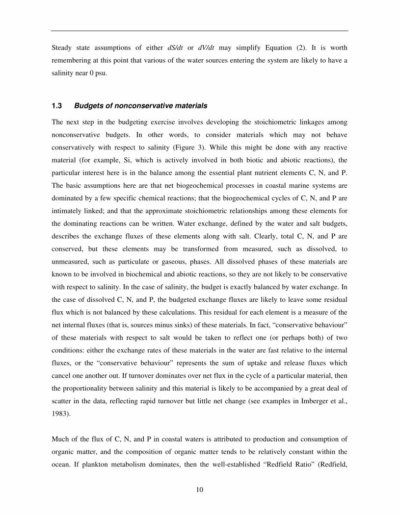
Steady state assumptions of either dS/dt or dV/dt may simplify Equation (2). It is worth

remembering at this point that various of the water sources entering the system are likely to have a

salinity near 0 psu.

1.3 Budgets of nonconservative materials

The next step in the budgeting exercise involves developing the stoichiometric linkages among

nonconservative budgets. In other words, to consider materials which may not behave

conservatively with respect to salinity (Figure 3). While this might be done with any reactive

material (for example, Si, which is actively involved in both biotic and abiotic reactions), the

particular interest here is in the balance among the essential plant nutrient elements C, N, and P.

The basic assumptions here are that net biogeochemical processes in coastal marine systems are

dominated by a few specific chemical reactions; that the biogeochemical cycles of C, N, and P are

intimately linked; and that the approximate stoichiometric relationships among these elements for

the dominating reactions can be written. Water exchange, defined by the water and salt budgets,

describes the exchange fluxes of these elements along with salt. Clearly, total C, N, and P are

conserved, but these elements may be transformed from measured, such as dissolved, to

unmeasured, such as particulate or gaseous, phases. All dissolved phases of these materials are

known to be involved in biochemical and abiotic reactions, so they are not likely to be conservative

with respect to salinity. In the case of salinity, the budget is exactly balanced by water exchange. In

the case of dissolved C, N, and P, the budgeted exchange fluxes are likely to leave some residual

flux which is not balanced by these calculations. This residual for each element is a measure of the

net internal fluxes (that is, sources minus sinks) of these materials. In fact, “conservative behaviour”

of these materials with respect to salt would be taken to reflect one (or perhaps both) of two

conditions: either the exchange rates of these materials in the water are fast relative to the internal

fluxes, or the “conservative behaviour” represents the sum of uptake and release fluxes which

cancel one another out. If turnover dominates over net flux in the cycle of a particular material, then

the proportionality between salinity and this material is likely to be accompanied by a great deal of

scatter in the data, reflecting rapid turnover but little net change (see examples in Imberger et al.,

1983).

Much of the flux of C, N, and P in coastal waters is attributed to production and consumption of

organic matter, and the composition of organic matter tends to be relatively constant within the

ocean. If plankton metabolism dominates, then the well-established “Redfield Ratio” (Redfield,

11

1934) is likely to be a reasonable approximation of the C:N:P ratio of locally produced (or

consumed) organic matter. If the system metabolism is dominated by seagrass or benthic algal

metabolism, then some other composition may be more appropriate (Atkinson and Smith, 1983).

For systems in which sedimentary materials apparently dominate the local reaction, or in which

particle inputs and outputs can be assumed to be small, then the sediment composition may be an

appropriate compositional ratio to consider. In any case, some estimate can be made of the local

organic matter composition. For the sake of linking the C, N, and P budgets, phosphorus may be

considered to have the simplest chemical pathways. All phosphorus in the system can be considered

to be in either the dissolved phase or the particulate phase, and phosphorus reactions involve

transfers between these phases; there is no gas phase. In contrast, both nitrogen and carbon have

prominent gas phases, and carbon and nitrogen fluxes involving the gas phases are known to be

important in coastal systems. The working assumption is therefore made that the internal reaction

flux of phosphorus is proportional to production and consumption of particulate material (generally

dominated by organic matter). That is, phosphorus moves back and forth between dissolved and

particulate material. N:P and C:P flux ratios are calculated from the budgetary analyses, and

deviations of these flux ratios from proportionality with respect to the particle composition are

attributed to gas-phase reactions for nitrogen and carbon.

Residual Y fluxF Y ; Y =(Y +Y )/2R R R 1 2

.

Precipitation (F )

(Y )P

P

Evaporation (F )

(Y =0)E

E

Runoff (Y )

Groundwater (Y )

Other (Y )

Q

G

O

COASTAL WATERBODY

Mixing Y fluxF (Y -Y )x 1 2

.

Ocean Concentration (Y )2

Net internal source or sink

Y∆

Air-Sea exchange for materials with

an active gas phase y∆ g

Figure 3. The budget for a non-conservative material, Y, in a coastal water body (Gordon et al., 1996).

Two other cautions are in order here. Firstly, it was pointed out above that water input from

processes like groundwater and sewage could often be ignored, and that the contributions of these

12

terms to the salt balance could likewise usually be ignored. It is clearly not the case that the nutrient

content of this water can be ignored; that should never be done for systems receiving significant

sewage input and should be done only with some caution for groundwater and precipitation. If there

is runoff, the nutrient input from that runoff must be included in the budget. Secondly, the budgets

present here generally involve only dissolved materials. While there are methods to construct very

useful budgets for particle fluxes, for example, sediment input by streams and deposition within the

system, in general, salinity-based budgets must be treated with great caution in constructing budgets

for particulate materials in shallow water systems. The reason is relatively simple. Dissolved

materials have no gravitational component of flux within the water while particles do. Therefore

particle distribution in the water column is likely to be extremely “patchy,” with respect to both

time and space, in areas subject to heavy loading with stream sediments, as well as in systems

where wave mixing or active bioturbation is stirring the bottom sediments up into the water column.

These processes can generate great heterogeneity in estimates of particle concentrations. While

budgetary calculations for particles can be made according to the procedures to be outlined here,

sampling artifacts may make the results quantitatively unreliable. As a result, the use of salt and

water balance calculations are not generally useful to estimate particle budgets. It is worth recalling,

however, that conservation of mass is a fundamental law of nature. Therefore, for materials without

a gas phase, any deviation of dissolved forms of that material from conservative behaviour must

represent net uptake or release with respect to particles. This point is used in the interpretation of

output from the budgets.

In this context, there are two stoichiometries to be considered in the LOICZ budget: (1) Nitrogen-Phosphorous stoichiometry: Nitrogen is present predominantly in seawater in the

gaseous from. Conversion of N2 gas to organic nitrogen is termed nitrogen fixation (nfix)

whereas conversion from NO3

-

to N2 is termed denitrification (denit). Both of these processes

require biotic mediation (bacteria) and usually require anaerobic conditions to proceed in

aqueous ecosystems. Significant amounts of nitrogen are transferred between the so-called fixed

nitrogen (DIN, DON (Dissolved Organic Nitrogen), PN (Particulate Nitrogen)), which is

normally measured and gaseous nitrogen (N2), which is not. The net effect of this transfer has

been termed by LOICZ as (nfix-denit). This value is often significant for the nitrogen budget,

for this reason LOICZ methodology has proposed the following methodology to calculate it

(Webb, 1981):

13

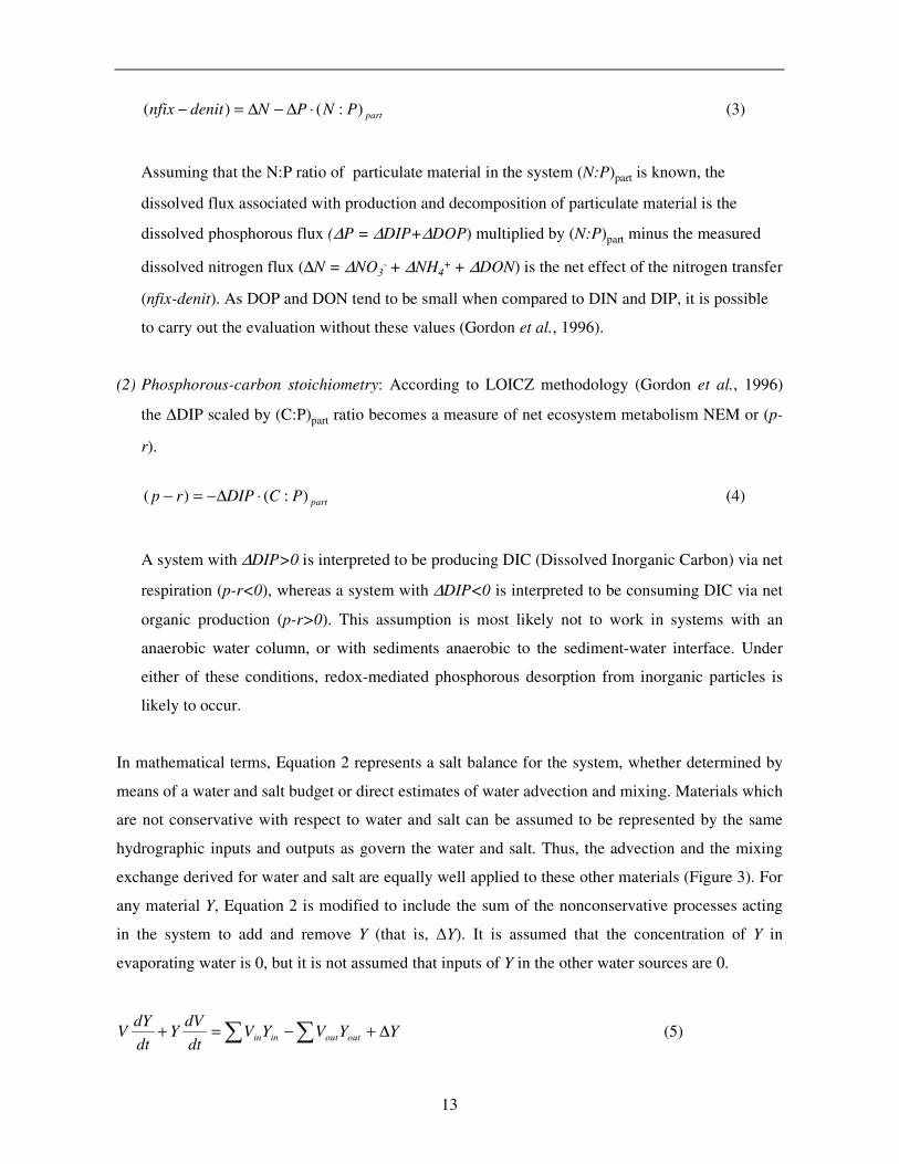
partPNPNdenitnfix ):()( ⋅∆−∆=− (3)

Assuming that the N:P ratio of particulate material in the system (N:P)part is known, the

dissolved flux associated with production and decomposition of particulate material is the

dissolved phosphorous flux (∆P = ∆DIP+∆DOP) multiplied by (N:P)part minus the measured

dissolved nitrogen flux (∆N = ∆NO3- + ∆NH4

+ + ∆DON) is the net effect of the nitrogen transfer

(nfix-denit). As DOP and DON tend to be small when compared to DIN and DIP, it is possible

to carry out the evaluation without these values (Gordon et al., 1996).

(2) Phosphorous-carbon stoichiometry: According to LOICZ methodology (Gordon et al., 1996)

the ∆DIP scaled by (C:P)part ratio becomes a measure of net ecosystem metabolism NEM or (p-

r).

partPCDIPrp ):()( ⋅∆−=− (4)

A system with ∆DIP>0 is interpreted to be producing DIC (Dissolved Inorganic Carbon) via net

respiration (p-r<0), whereas a system with ∆DIP<0 is interpreted to be consuming DIC via net

organic production (p-r>0). This assumption is most likely not to work in systems with an

anaerobic water column, or with sediments anaerobic to the sediment-water interface. Under

either of these conditions, redox-mediated phosphorous desorption from inorganic particles is

likely to occur.

In mathematical terms, Equation 2 represents a salt balance for the system, whether determined by

means of a water and salt budget or direct estimates of water advection and mixing. Materials which

are not conservative with respect to water and salt can be assumed to be represented by the same

hydrographic inputs and outputs as govern the water and salt. Thus, the advection and the mixing

exchange derived for water and salt are equally well applied to these other materials (Figure 3). For

any material Y, Equation 2 is modified to include the sum of the nonconservative processes acting

in the system to add and remove Y (that is, ∆Y). It is assumed that the concentration of Y in

evaporating water is 0, but it is not assumed that inputs of Y in the other water sources are 0.

∑ ∑ ∆+−=+ YYVYVdt

dVY

dt

dYV outoutinin (5)

14

Again, steady state assumptions may allow one or both of the derivatives on the left side of the

equation to be dropped. In some cases individual fluxes may be directly available, rather than being

the product of concentration and flow. For example, sewage input of Y may be directly known,

without data on sewage volume. The summed nonconservative fluxes (∆Y) are the information

desired and are derived by rearrangement:

∑ ∑+−+=∆ outoutinin YVYVdt

dVY

dt

dYVY (6)

The units of ∆Y are mass per time; generally presented in this report as moles (mol) or kilomoles

per day. Note two aspects of this equation. In the first place, this derivation gives no information

about the processes leading to ∆Y, either the number of processes or the general form of those

processes. Physical, abiotic chemical, or biotic chemical processes may contribute to ∆Y, and they

are indistinguishable from this derivation. Such information is derived through other considerations,

as discussed in the next section and exemplified in the case studies. Some terms, again sewage is an

example, may be directly entered as known values in Equation 6, or may be part of the term ∆Y.

In the second place, while this budgeting procedure based on a salt balance is in principle applicable

to any material in many situations, it often cannot be applied with much quantitative success to

particulate materials. The concentrations of these materials tend to be so patchy both spatially and

temporally in response to sedimentation and resuspension that they are not adequately sampled in

the context of a budgetary procedure derived for application to tidally averaged data.

In general is useful to express ∆Y per unit area, by dividing the value estimated according to

Equation 4 by the system area, often expressed as mol or mmol m-2

d-1

.

15

2. THE MEDITERRANEAN SEA BASIN

2.1 Study Area

Although making up merely 1% of the total world ocean surface, the Mediterranean Sea is often

used as a representative model of the world’s oceans to assess the global change of the

environment, due to its practically enclosed character. Thus, the Mediterranean Sea can be

considered an important laboratory basin for water cycle, climate change and biota response in

changing environments. The marked seasonal cycle, and in particular the timing and location of the

winter storms, affect the regional hydrology (Peixoto et al., 1982), its variability being also an

important prerequisite for a correct understanding of the Sea’s hydrology not only from an

environmental but also from a socio-economic standpoint.

The Mediterranean Sea stretches at its widest cross-sections about 4,000 km and 900 km from west

to east and south to north, respectively (Laubier, 2005). The surface area and volume are

approximately 2.51x1012 m2 and 4.67x106 km3, respectively. The average depth is approximately

1,500 m. It is connected to the Black Sea via the Strait of Dardanelles (7 km width and 55 m

average depth) and to the Atlantic Ocean via the Strait of Gibraltar (15 km width and 290 m deep

sill). An artificial connection to the Red Sea is given through the Suez Canal. More than 130 million

people live on a permanent basis along the Mediterranean coastline, this figure doubling during the

summer tourist season (EEA, 2005). Figure 4 shows the topography of the Mediterranean Sea for an

appreciation of its spatial depth distribution.

Figure 4. Topography of the Mediterranean Sea. The 1000 m contour is shown, and regions deeper than 3000 m are shaded. The 200 m contour is shown as a broken line where it departs significantly from the 1000 m contour. In addition, the 2000 m contour is shown as a broken line in the Black Sea (adopted from Tomczak and Godfrey (2003)).

16

The Mediterranean climate is marked by high winter and low summer precipitation, where the

summer rainfall accounts for less than 10 percent of the annual total. A north-to-south gradient of

the mean annual precipitation is evident, with precipitation decreasing towards the south. Especially

in the Alpine and Pyrenean headwater areas, high precipitation (1,500 – 2,000 mm/yr) can be

encountered. Thus, in the northern Mediterranean, the principal rivers are recharged via rather big

basins, while the smaller basins usually experience floods. In the southern Mediterranean, on the

other hand, there is a prevalence of very small rivers and flash floods are generally common

(Laubier, 2005). In addition, the Mediterranean region is considered one of the most sensitive

regions on Earth in the context of climate change as a consequence of its position between two

different climate regimes in the North and the South (Somot et al., 2006).

The largest river inflows come from the Nile, Rhône, Po and Ebro. The total riverine input to the

Mediterranean Sea has been very roughly estimated at about 473 billion m3/year (EEA/UNEP,

1999). For most parts of the Mediterranean Sea, evaporation exceeds the precipitation and river

runoff inputs by over a 1 m, thereby causing a negative overall water budget. Thus, the

Mediterranean Sea is often called an “evaporation basin”, as it has a negative balance with the

Atlantic Ocean. Thus the Mediterranean Sea can be considered a concentration basin. Theoretically,

the sea level in the Mediterranean would decrease at a rate of about 0.5-1.0 m/yr if the Strait of

Gibraltar became closed (Laubier, 2005). A consequence of this greater evaporation is that the

water salinity increases, causing in the end a decrease in water temperature. Consequently, the two

driving forces in the Mediterranean Sea which are responsible for the inflow of Atlantic surface

water and the outflow of the Mediterranean deep water are the freshwater deficit and density

increase. Generally speaking, the exchange between the Mediterranean Sea and the Atlantic Ocean

occurs as the more saline and denser Mediterranean deep waters go out to the Atlantic Ocean, while

the lighter Atlantic surface waters enter. The residence time for water entering through the Strait of

Gibraltar is estimated to be between 80 and 200 years (Hopkins, 1999).

In the Mediterranean Sea, there are relatively strong vertical and lateral currents, therefore enabling

relatively rapid mixing of introduced contaminants from the air, land or water compartments. The

residence time for a basin is considered to be one of the indicators of how long contaminants may

amass in a basin before mixing and then exiting a basin. The turnover time for the entire

Mediterranean basin is estimated to range between 200 and 300 years (UNEP/MAP/MED POL,

2004).

17

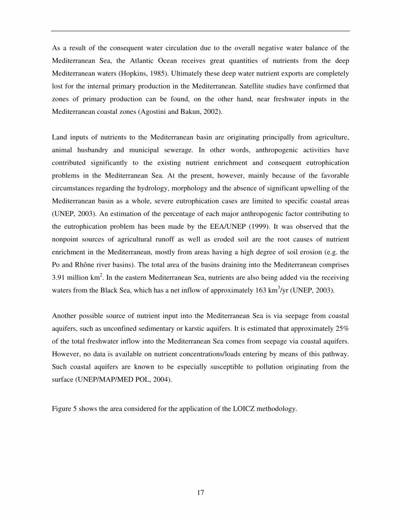
As a result of the consequent water circulation due to the overall negative water balance of the

Mediterranean Sea, the Atlantic Ocean receives great quantities of nutrients from the deep

Mediterranean waters (Hopkins, 1985). Ultimately these deep water nutrient exports are completely

lost for the internal primary production in the Mediterranean. Satellite studies have confirmed that

zones of primary production can be found, on the other hand, near freshwater inputs in the

Mediterranean coastal zones (Agostini and Bakun, 2002).

Land inputs of nutrients to the Mediterranean basin are originating principally from agriculture,

animal husbandry and municipal sewerage. In other words, anthropogenic activities have

contributed significantly to the existing nutrient enrichment and consequent eutrophication

problems in the Mediterranean Sea. At the present, however, mainly because of the favorable

circumstances regarding the hydrology, morphology and the absence of significant upwelling of the

Mediterranean basin as a whole, severe eutrophication cases are limited to specific coastal areas

(UNEP, 2003). An estimation of the percentage of each major anthropogenic factor contributing to

the eutrophication problem has been made by the EEA/UNEP (1999). It was observed that the

nonpoint sources of agricultural runoff as well as eroded soil are the root causes of nutrient

enrichment in the Mediterranean, mostly from areas having a high degree of soil erosion (e.g. the

Po and Rhône river basins). The total area of the basins draining into the Mediterranean comprises

3.91 million km2. In the eastern Mediterranean Sea, nutrients are also being added via the receiving

waters from the Black Sea, which has a net inflow of approximately 163 km3/yr (UNEP, 2003).

Another possible source of nutrient input into the Mediterranean Sea is via seepage from coastal

aquifers, such as unconfined sedimentary or karstic aquifers. It is estimated that approximately 25%

of the total freshwater inflow into the Mediterranean Sea comes from seepage via coastal aquifers.

However, no data is available on nutrient concentrations/loads entering by means of this pathway.

Such coastal aquifers are known to be especially susceptible to pollution originating from the

surface (UNEP/MAP/MED POL, 2004).

Figure 5 shows the area considered for the application of the LOICZ methodology.

18

2.2 Data Provision

In order to perform the LOICZ budgeting approach to the Mediterranean Sea numerous input data

were necessary. In addition, a preliminary watershed modelling exercise was indispensable in order

to obtain an estimate of the total streamflow and nutrient inputs originating from the land surface

into the Sea. The details of these model simulations and the related data sources have already been

described in Strobl et al. (2008). The fluxes considered in the budgets were for streamflow, SGD,

precipitation (wet and dry deposition) as well as interchange fluxes between the Mediterranean Sea

and its neighbouring water bodies (i.e., Atlantic Ocean and Black Sea). The water budget included

additionally the evaporation loss. No other input sources were considered. Table 1 depicts a

summary of the data used for the LOICZ budget of the Mediterranean Sea.

Water budget input data

The AVGWLF model was used to estimate the total streamflow input for the time period 1996-

2005 into the Mediterranean Sea. For the simulation, the watershed contributing areas to the

Mediterranean Sea were divided into 65 units, and subsequently the computed streamflow was

totalled from all units and added to an estimate for the Nile river of 3.91 ×1010 m3/yr (Global

Runoff Data Centre, 2008), which was not simulated with the AVGWLF model (see Strobl et al.,

N

EW

S

0 1000500km

N

EW

S

0 1000500km

0 1000500km

Figure 5. Boundary definitions for the LOICZ balance.

19

2008) and represents the mean annual value for the Nile river for the period 1973 to 1984. The

submarine groundwater discharge (SGD) to the Mediterranean Sea, on the other hand, was

estimated from a study by Zekster and Dzhamalov (1988) on the world’s oceans, and a time-

invariant value was applied in the LOICZ budget.

Table 1. Summary of data used for the LOICZ budget of the Mediterranean Sea.

Data Type Budget Reference Year(s) Spatial Reference Data Source

Streamflow Water 1996 - 2005 Land surface surrounding MED

AVGWLF Model Simulation (Evans

et al. 2008) Precipitation Water 1996 - 2005 Over MED

Evaporation Water 1996 - 2005 Over MED SGD Water 1988 MED Zektser and

Dzhamalov (1988) Inflow from ATL to

MED

Water 1991 MED-ATL Interface Bryden et al.

(1994) Outflow from MED

to ATL

Water 1991 MED-ATL Interface Bryden et al.

(1994) Inflow from

BLACK to MED

Water unknown MED-BLACK Interface Pickard and Emery

(1990) Outflow from MED

to BLACK

Water unknown MED-BLACK Interface Pickard and Emery

(1990)

Stream Salinity Salt n/a MED Assumed value SGD Salinity Salt 2002 Southeastern Sicily Povinec et al.

(2006) MED Salinity Salt 1874 - 2005 MED Antonov et al.

(2006) ATL Salinity Salt 1874 - 2005 ATL (area close to MED

interface)

Antonov et al.

(2006) BLACK Salinity Salt 1874 - 2005 BLACK (area close to

MED interface)

Antonov et al.

(2006) Stream DIN Nitrogen 1996 - 2005 Land surface surrounding

MED

AVGWLF Model

Simulation (Evans

et al., 2008)

SGD DIN Nitrogen 2002 Southeastern Sicily Povinec et al. (2006)

Deposition DIN Nitrogen 2001-03 Average of various sites in MED

Markaki et al. (2008)

MED DIN Nitrogen 1925 - 2005 MED Garcia et al. (2006)

ATL DIN Nitrogen 1925 - 2005 ATL (area close to MED interface)

Garcia et al. (2006)

BLACK DIN Nitrogen 1925 - 2005 BLACK (area close to MED interface)

Garcia et al. (2006)

Stream DIP Phosphorus 1996 - 2005 Land surface surrounding MED

AVGWLF Model Simulation (Evans

et al. 2008)

SGD DIP Phosphorus 2002 Southeastern Sicily Povinec et al.

(2006) Deposition DIP Phosphorus 2001-03 Average of various sites

in MED

Markaki et al.

(2008) MED DIP Phosphorus 1922 - 2005 MED Garcia et al. (2006)

ATL DIP Phosphorus 1922 - 2005 ATL (area close to MED interface)

Garcia et al. (2006)

BLACK DIP Phosphorus 1922 - 2005 BLACK (area close to MED interface)

Garcia et al. (2006)

Abbreviations: ATL = Atlantic Ocean; MED = Mediterranean Sea; BLACK = Black Sea; DIN = dissolved

inorganic nitrogen; DIP = dissolved inorganic phosphorus; SGD = submarine groundwater discharge.

20

Gridded precipitation-data sets are an essential base for many applications in geosciences and

especially in climate research, as for instance global and regional studies on the hydrological cycle

and on climate variability, verification and calibration of satellite based climate data or the

evaluation of global circulation models (GCMs). As all applications require reliable high quality

precipitation fields the underlying station data have to meet high demands concerning the quality of

the observed precipitation data as well as the correctness of station meta data and also with respect

to sufficient spatial station density and distribution. Concerning the use of regionally or globally

gridded climate data for analyses of long-term climate variability it has to be ensured that station

data used for gridding are as continuous and homogeneous as possible. In recent years various

globally gridded data-sets of monthly terrestrial precipitation observations have been developed for

example at the European Centre for Medium Range Weather Forecast (ECMWF), the National

Center for Environmental Prediction (NCEP) or the Global Precipitation Climatology Centre

(GPCC). For research purposes most of these data sets are available free of charge.

For the purpose of this study, model data from the reanalysis projects of ECMWF (ERA40) was

used. This is also due to fact, that the gridded precipitation product of GPCC is based on

measurement stations, which are located on land and are then extrapolated to cover the

Mediterranean Sea. Such an extrapolation must be considered as rather doubtful, as the situation

over sea is very different from that over land. Precipitation and evaporation estimates for the entire

Mediterranean Sea were therefore derived from the ERA-40 reanalysis datasets, for a detailed

description of the project see Uppala et al. (2005). This dataset is the results of a collective effort

based on the ERA-40 re-analysis project, carried out by the (ECMWF), in collaboration with a

number of institutions in Europe, Asia and North America. Very recently ECMWF has undertaken a

new reanalysis effort called ERA-Interim, which most important is covering an extended time

period going now until December 2008. The other for this study important point is that the complete

humidity analysis was redone and thereby hopefully improved.

Meteorological observation from a number of different sources (stations, satellite, aircraft,

radiosondes, ocean-buoys and other surface platforms), covering the period from September 1957 to

August 2002, were collected and a global data assimilation system was set up and operated during

the full period. These data are now available from the Meteorological Archival and Retrieval

System (MARS), which is the main data repository at ECMWF. From the available global data in

spectral representation an area covering the European area (25W-45E, 30S-67N) was selected and

then interpolated to a grid with unique resolution of 0.5 x 0.5 degrees. Large Scale Precipitation

21

(LSP) and Convective Precipitation (CP) where both downloaded and aggregated in order to

calculate Total Precipitation (TP). Evaporation (E) comprises evaporation and condensation. The

sign convention used here for the data conversion, is so that precipitation and condensation are

positive (water accumulation on land or sea), whereas real evaporation is negative (loss of water to

the atmosphere). This is opposite to the typical sign convention in meteorology, where precipitation

is considered a water loss of the atmosphere.

Precipitation and evaporation data as retrieved from MARS were accumulated into annual totals

from the 6-hourly data (0:00, 6:00, 12:00, 18:00) for the period 1996-2002. For the remainder of the

period (September 2002 to December 2005), pure model data derived from the operational model

(IFS) of ECMWF were used. For comparison a second set of annual accumulated precipitation and

evaporation data where calculated from the ERA-Interim product for the period from 1996 until

2008.

It should be mentioned that specifically the global modelling of precipitation despite the

considerable progress made during the last decade still contains large uncertainties (see e.g.

Troccoli and Kållberg, 2004) and even the measured data are not completely satisfactory. A recent

model intercomparison of GCM’s demonstrated that differences of up to 100% occurred (SCOR

working group on fluxes and Turk et al. 2008). Fortunately, the most severe problems are apparent

in the tropics and the southern hemisphere, whereas the arid climate of the Mediterranean Sea gives

much more reliable precipitation estimates.

Estimates for the water exchange fluxes between the Mediterranean and Black Seas as well as

between the Mediterranean Sea and Atlantic Ocean were obtained from Pickard and Emery (1990)

and Bryden et al. (1994), respectively. These annual estimates were applied to all years in the time

period of 1996-2005.

Salt budget input data

As no estimates for the salinity of incoming streamflow for the Mediterranean Sea were available,

an average salinity value of 5 psu was assumed for the streamflow entering the Mediterranean Sea

for the entire budget time period. The salinity of the SGD was estimated on basis of salinity

measured in southeastern Sicily in the Donnalucata area (see Figure 6). Due to lack of better

measured data, this value was used for the entire budget time period and for the entire

Mediterranean Sea. The World Ocean Database 2005 (Antonov et al., 2006), on the other hand, was

22

used to estimate the salinities for the Mediterranean and Black Seas as well as for the Atlantic

Ocean. An average was calculated from 33 standard depths (from 0 m to 5500 m) using one degree

gridded data. For the Black Sea and the Atlantic Ocean, only the sea/ocean areas near the

Mediterranean interface were used in the calculations of the average salinity (within ca. 250 km of

the interfaces).

Nitrogen budget input data

The AVGWLF model was used to estimate nitrogen load (as dissolved nitrogen) coming from the

streams draining into the Mediterranean Sea (the Nile river was not included in the simulations). It

was assumed that dissolved nitrogen represented mainly dissolved inorganic nitrogen (DIN).

Dissolved nitrogen concentrations of SGD to the Mediterranean Sea were taken from nitrate

estimates of the study by Povinec et al. (2006), representing the southeastern area of Sicily.

Dissolved nitrogen estimates for precipitation (wet and dry deposition) falling on the Mediterranean

Sea were obtained as an average from DIN measurements between 2001 and 2003 of ten coastal

measuring points spread over the Mediterranean (see Figure 6). These measurements were

performed in a study by Markaki et al. (2008) and were taken as far as possible from any local and

regional influences in order that the results could be considered representative of long range

0 1000500km

N

EW

S

Submarine Groundwater Discharge Measurement Point

Deposition Measurement Point

0 1000500km

0 1000500km

N

EW

S

Submarine Groundwater Discharge Measurement Point

Deposition Measurement Point

Figure 6. Nutrient deposition and SGD measurement points used for the LOICZ budget of the Mediterranean Sea.

23

transport and open sea deposition conditions. These estimates were assumed to be valid for the time

period of 1996 to 2005. Similarly to the salinity estimates, the dissolved nitrogen estimates for the

Mediterranean and Black Seas as well as for the Atlantic Ocean were computed from the World

Ocean Database 2005 (Garcia et al., 2006) where an average value was computed from 33 standard

depths using one degree gridded data.

Phosphorus budget input data

As for the nitrogen budget, the AVGWLF model was utilized to obtain an estimate of the dissolved

phosphorus (DP) coming from the land surface draining into the Mediterranean Sea. The DP

originating from the SGD was estimated, similarly as for the DN estimate, from the study by

Povinec et al. (2006) for southeastern Sicily and assumed to be applicable for the entire

Mediterranean basin. The estimates of DP for wet and dry deposition were obtained from the study

by Markaki et al. (2008). Computations from the data from the World Ocean Database 2005

(Garcia et al., 2006) were performed to obtain an estimate for DP present in the Black and

Mediterranean Seas and Atlantic Ocean and assumed to be representative for the time period of

1996 to 2005.

24

3. LOICZ BUDGET OF THE MEDITERRANEAN SEA

3.1 Water Budget

The water budget can be written as:

bRaRbRaROGEPQ

sysFFFFFFFFF

dt

dV2211 +−−+++−+= (7)

where Vsys refers to the Mediterranean Sea volume, FQ represents the inflows from stream runoff,

FP is the flow due to direct precipitation, FE is the loss due to evaporation, FG refers to the

submarine groundwater discharge, FO refers to other inflows such as sewage, and FR1a and FR2b are

the flows due to hydrographically driven advective inflow from the Atlantic Ocean and Black Sea,

respectively. Removals include evaporation, FE, and advective outflow of water from the system

into the Atlantic Ocean and Black Sea, FR1b and FR2a, respectively. It is useful to consider the

difference between the incoming (Fin = FR1a + FR2b) and outgoing (Fout = FR1b + FR2a) advective

f.lows into the system (i.e., the Mediterranean Sea) as the residual flow (FR) driven by the water

budget, see Figure 1. In fact, FR can be obtained assuming dVsys/dt = 0 as:

OGEPQoutinR FFFFFFFF −−+−−=−= (8)

Figure 7 shows a semi-schematic of the system under consideration along with the exchange fluxes

considered in the budget of the Mediterranean Sea.

A comparison of the estimated amounts of streamflow, precipitation and evaporation over the Sea

(Figure 8) confirms the well known fact that evaporation on average greatly exceeds precipitation

by more than twice the amount, and even more so streamflow to the Mediterranean Sea (Mariotti et

al., 2002). This observation is quite central to the water circulation within the basin.

Table 2 shows the water budget for the Mediterranean Sea.

25

Figure 7. Semi-schematic of the system under consideration for the budget (where ATL = Atlantic Ocean; MED = Mediterranean Sea; BLACK = Black Sea; FR1a = incoming flow from ATL to MED; FR1b = outgoing flow from MED to ATL; FR2a = outgoing flow from MED to BLACK; FR2b = incoming flow from BLACK to MED).

1996 1997 1998 1999 2000 2001 2002 2003 2004 2005Time (year)

1.0x1012

2.0x1012

3.0x1012

4.0x1012

Q, P and E (m

3/year)

LegendEvaporation (E)

Precipitation (P)

Streamflow (Q)

Figure 8. Estimated streamflow, precipitation and evaporation for the Mediterranean Sea.

MED

BLACK

ATLFR1a

FR1b

FR2a

FR2b

MED

BLACK

ATLFR1a

FR1b

FR2a

FR2b

26

Table 2. Water budget for the Mediterranean Sea.

Year FQ (m3) FP (m

3) FE (m

3) FG (m

3) FO (m

3) FR1a (m

3) FR1b (m

3) FR1 (m

3) FR2a (m

3) FR2b (m

3) FR2 (m

3) FR (m

3)

1996 5.32E+11 1.29E+12 -2.85E+12 1.40E+08 0 2.16E+13 -2.29E+13 -1.33E+12 -1.90E+11 4.11E+11 2.21E+11 -1.11E+12 1997 3.84E+11 1.08E+12 -2.87E+12 1.40E+08 0 2.15E+13 -2.28E+13 -1.32E+12 -1.89E+11 4.10E+11 2.21E+11 -1.10E+12 1998 3.96E+11 9.74E+11 -2.92E+12 1.40E+08 0 2.15E+13 -2.28E+13 -1.32E+12 -1.89E+11 4.10E+11 2.21E+11 -1.10E+12 1999 3.58E+11 9.28E+11 -2.97E+12 1.40E+08 0 2.15E+13 -2.28E+13 -1.32E+12 -1.89E+11 4.10E+11 2.21E+11 -1.10E+12 2000 3.46E+11 8.73E+11 -2.99E+12 1.40E+08 0 2.16E+13 -2.29E+13 -1.33E+12 -1.90E+11 4.11E+11 2.21E+11 -1.11E+12 2001 3.58E+11 9.70E+11 -3.10E+12 1.40E+08 0 2.15E+13 -2.28E+13 -1.32E+12 -1.89E+11 4.10E+11 2.21E+11 -1.10E+12 2002 4.09E+11 1.11E+12 -2.87E+12 1.40E+08 0 2.15E+13 -2.28E+13 -1.32E+12 -1.89E+11 4.10E+11 2.21E+11 -1.10E+12 2003 3.99E+11 1.23E+12 -2.87E+12 1.40E+08 0 2.15E+13 -2.28E+13 -1.32E+12 -1.89E+11 4.10E+11 2.21E+11 -1.10E+12 2004 4.34E+11 1.10E+12 -3.01E+12 1.40E+08 0 2.16E+13 -2.29E+13 -1.33E+12 -1.90E+11 4.11E+11 2.21E+11 -1.11E+12 2005 4.18E+11 1.05E+12 -3.16E+12 1.40E+08 0 2.15E+13 -2.28E+13 -1.32E+12 -1.89E+11 4.10E+11 2.21E+11 -1.10E+12

Table 3. Overall flow exchange as computed from Pickard and Emery (1990) and Bryden et al. (1994) as well as from Equation 7.

Source Pickard and Emery (1990) & Bryden et al. (1994)

Equation 7

Year FR (m

3) FR (m

3) Difference (m

3)

1996 -1.11E+12 -1.03E+12 -7.42E+10 1997 -1.10E+12 -1.41E+12 3.02E+11 1998 -1.10E+12 -1.55E+12 4.51E+11 1999 -1.10E+12 -1.68E+12 5.77E+11 2000 -1.11E+12 -1.77E+12 6.59E+11 2001 -1.10E+12 -1.78E+12 6.73E+11 2002 -1.10E+12 -1.35E+12 2.43E+11 2003 -1.10E+12 -1.24E+12 1.32E+11 2004 -1.11E+12 -1.48E+12 3.71E+11 2005 -1.10E+12 -1.70E+12 5.92E+11

27

Using the streamflow estimates of the AVGWLF model simulation along with the precipitation and

evaporation data from the reanalysis projects of ECMWF (ERA40), as well as the SGD estimates, a

water budget for the time period 1996 to 2005 could be undertaken. However, using these input

parameters only, merely permits the computation of the overall exchange (i.e., FR) between the

system (i.e. the Mediterranean Sea) and its neighbouring water bodies (the Atlantic Ocean and

Black Sea). In order to achieve this, the term dVsys/dt in Equation 3 is assumed to tend to zero. This

assumption is justifiable as the water budget has been performed on an annual basis. Nonetheless,

using only these data does not allow for a more accurate evaluation of the term FR. In other words,

the incoming and outgoing flows between the Mediterranean Sea and the Atlantic Ocean and Black

Sea cannot be obtained. However, Pickard and Emery (1990) and Bryden et al. (1994) have

estimated these incoming and outgoing flows for the Black Sea and Atlantic Ocean, respectively

(see Table 2). Table 3 shows the overall flow exchange for the Mediterranean Sea using Pickard

and Emery’s (1990) and Bryden et al.’s (1994) estimates as well as a comparison of the FR as

calculated via Equation 7. As can be observed, the differences for the time period 1996 to 2005

range from absolute values of approximately 4·1010 to 6·1011 m3/yr. This represents differences of

one to two magnitudes lower than the estimated values and can be considered to be within

acceptable limits for a water budget calculation for the Mediterranean basin.

On an annual basis, it is seen from Table 2 that the Mediterranean Sea has an overall water addition

from the Black Sea and water loss to the Atlantic Ocean. Table 2 also shows that the major water

flows into and out of the Mediterranean basin are from the interface with the Atlantic Ocean.

3.2 Salt Budget

The salt budget can be written as:

BLACKbRsysaRsysbRATLaROOGGQQ

sys

sys SFSFSFSFSFSFSFdt

dSV 2211 +−−+++= (9)

where Ssys refers to the Mediterranean Sea salinity, SQ is the salinity of the incoming streamflows,

SG refers to the salinity of the submarine groundwater discharge, SO is the salinity of other incoming

flows (e.g. sewage flow), SATL is the salinity of the Atlantic Ocean at the Strait of Gibraltar, and

SBLACK is the salinity of the Black Sea near the entrance to the Mediterranean Sea. In this equation,

28

the mixing terms Fin and Fout remain as the unknowns. It was assumed that the salinity input due to

deposition was negligible.

Using the salinity estimates available for the Mediterranean system, a salt budget was performed

and is presented in Table 4.

Table 4. Salt budget for the Mediterranean Sea.

Year SQ (psu) SG (psu) SO (psu) Ssys (psu) SATL(psu) SBLACK (psu) dt

dS sys

(psu)

1996 5.00E+00 3.70E+01 0.00E+00 3.86E+01 3.59E+01 2.12E+01 -2.25E-02 1997 5.00E+00 3.70E+01 0.00E+00 3.86E+01 3.59E+01 2.12E+01 -2.26E-02 1998 5.00E+00 3.70E+01 0.00E+00 3.86E+01 3.59E+01 2.12E+01 -2.26E-02 1999 5.00E+00 3.70E+01 0.00E+00 3.86E+01 3.59E+01 2.12E+01 -2.26E-02 2000 5.00E+00 3.70E+01 0.00E+00 3.86E+01 3.59E+01 2.12E+01 -2.27E-02 2001 5.00E+00 3.70E+01 0.00E+00 3.86E+01 3.59E+01 2.12E+01 -2.26E-02 2002 5.00E+00 3.70E+01 0.00E+00 3.86E+01 3.59E+01 2.12E+01 -2.25E-02 2003 5.00E+00 3.70E+01 0.00E+00 3.86E+01 3.59E+01 2.12E+01 -2.26E-02 2004 5.00E+00 3.70E+01 0.00E+00 3.86E+01 3.59E+01 2.12E+01 -2.26E-02 2005 5.00E+00 3.70E+01 0.00E+00 3.86E+01 3.59E+01 2.12E+01 -2.25E-02

The calculation ofdt

dS sysin Table 4 confirms that the estimated salinity values for streamflow, SGD,

etc. along with the computed salinity values computed for the Mediterranean Sea, Atlantic Ocean

and Black Sea from the World Ocean Database 2005 data are acceptable as the long-term expected

change in the system should approach zero. It can also be observed that the salinity of the Black Sea

is less than that of the Atlantic Ocean and Mediterranean Sea. Due to the high evaporation and low

runoff from streams, the salinity value for the Mediterranean Sea is much higher than for the Black

Sea. This is also can be explained from the fact that the Mediterranean Sea is a concentration basin,

whereas the Black Sea is considered a dilution basin since it receives great freshwater inputs from

the Danube river. However, it should be noted that there a few parts of the Mediterranean Sea that

receive great freshwater input, such as the Adriatic Sea from the Po river, which hence locally

represents a dilution basin.

3.3 DIP Balance

The following equation represents a mass balance for the system in the case where compound(s)

undergo chemical transformations inside the coastal lagoon:

29

YYFYFYFYFYFYFYFYFdt

dYV BLACKbRsysaRsysbRATLaROOGGPPQQ

sys

sys ∆++−−++++= 2211 (10)

where Y refers to the concentration of the species, and ∆Y represents the net internal source or sink.

The definition of the subscripts is as previously defined. In this case we are interested in the last

term of Equation 10 which will give us an idea on the behaviour of our system, i.e. sink or source,

in relation to a particular species. However, it is clear that R is the sum of all processes (physical,

chemical or biological) taking place, i.e.:

∑=

⋅=

n

i

ii rR1

ν (11)

where νi is the stoichiometric coefficient for the i-th transformation, and hence, in principle, the

mass balance will not give us any information concerning the number of processes (n) and their

relative importance (ri/rj).

In order to estimate the dissolved inorganic phosphorous for the Mediterranean Sea, the AVGWLF

model (Evans et al., 2008) has been employed as reported in Strobl et al. (in press). DP

concentrations were assumed to be approximately equal to DIP concentrations and indeed this is

usually the case. The calculated annual mean dissolved phosphorous loads in streamflow entering

the Mediterranean Sea for the period 1996 to 2005 can be seen in Figure 9.

∆DIP is therefore calculated in the following manner:

BLACKbRHsysaR

sysbRATLaROOGGPPQQ

sys

sys

sys

sys

DIPFDIPF

DIPFDIPFDIPFDIPFDIPFDIPFdt

dDIPV

S

VRDIP

⋅−⋅+

⋅+⋅−⋅−⋅−⋅−⋅−=⋅

=∆

22

11

(12)

The calculated ∆DIP budget for the Mediterranean Sea is shown in Table 5. As can be seen, for the

selected time period the estimated ∆DIP is relatively constant. On a yearly basis, the Mediterranean

Sea acts as a sink of phosphorous. For a more precise definition of a general behaviour throughout

different periods of the year, a monthly or seasonal balance would have been required. A graphical

representation of ∆DIP for the time period 1996 to 2005 is shown in Figure 10.

30

1996 1997 1998 1999 2000 2001 2002 2003 2004 2005Time (year)

1.0x107

1.5x107

2.0x107

2.5x107

3.0x107

Dissolved P (kg)

2.0x108

3.0x108

4.0x108

5.0x108

Dissolved N (k

g)

Legend

DP (kg)

DN (kg)

Figure 9. Calculated annual amount of dissolved phosphorous and dissolved nitrogen (in kg)

discharged to the Mediterranean Sea from its catchments.

Table 5. ∆DIP and ∆DIN budgets for the Mediterranean Sea for the time period 1996 to 2005.

Year ∆DIP (kg/yr) ∆DIP

(mmol/m2/d)

∆DIN (kg/yr) ∆DIN

(mmol/m2/d)

1996 4.05E+08 1.38E-02 4.26E+09 3.32E-01 1997 3.96E+08 1.35E-02 4.11E+09 3.20E-01 1998 3.97E+08 1.35E-02 4.14E+09 3.23E-01 1999 3.93E+08 1.34E-02 4.07E+09 3.17E-01 2000 3.96E+08 1.35E-02 4.07E+09 3.17E-01 2001 3.96E+08 1.35E-02 4.11E+09 3.20E-01 2002 3.96E+08 1.35E-02 4.12E+09 3.21E-01 2003 3.95E+08 1.35E-02 4.13E+09 3.22E-01 2004 4.01E+08 1.36E-02 4.17E+09 3.25E-01 2005 4.02E+08 1.37E-02 4.15E+09 3.23E-01

31

1996 1997 1998 1999 2000 2001 2002 2003 2004 2005

Time (year)

1.30x10-2

1.32x10-2

1.34x10-2

1.36x10-2

1.38x10-2

1.40x10-2

�DIP (mmol/m

2/d)

3.10x10-1

3.20x10-1

3.30x10-1

3.40x10-1

�DIN (m

mol/m

2/d)

Legend

�DIP

�DIN

Figure 10. Estimated ∆DIP and ∆DIN for the time period 1996 to 2005.

3.4 DIN Balance

In order to carry out a mass balance of dissolved inorganic nitrogen (DIN) for the Mediterranean

Sea, Equation 10 has been rearranged accordingly:

BLACKbRHsysaR

sysbRATLaROOGGPPQQ

sys

sys

sys

sys

DINFDINF

DINFDINFDINFDINFDINFDINFdt

dDINV

S

VRDIN

⋅−⋅+

⋅+⋅−⋅−⋅−⋅−⋅−=⋅

=∆

22

11

(13)

Table 5 and Figure 9 show the estimated ∆DIN budget for the period of 1996 to 2005. Similarly to

the ∆DIP budget the annual mean values remain constant throughout the selected time period. The

budget shows that on an annual basis, the Mediterranean Sea can be considered a sink of nitrogen.

For the DIN there is no specific trend, similarly to the case of DIP.

32

3.5 Stoichiometrically Linking the Nonconservative Budgets

One procedure to gain insight into the main processes responsible for the non-conservative fluxes is

to study the relationships between them and to see if it is possible to link them stoichiometrically

according to well-known processes in the coastal zone. In the case of the whole Mediterranean, we

can assume that plankton metabolism dominates, then the “Redfield Ratio” is likely to be a

reasonable approximation of the C:N:P ratio of locally produced (or consumed) organic matter.

Figure 11 shows the variation of nfix-dnit for the selected 10-year time period, as well as the

corresponding production-respiration NEM (Net Ecosystem Metabolism) balance. As can be

observed, the Mediterranean Sea shows a positive balance between nitrogen fixation and

denitrification during the analyzed years. On the contrary, NEM is always negative indicating that

there is a net production of dissolved inorganic carbon (DIC).

It is important to underline that the linking of stoichiometric budgets, due to the absence of relevant

data, is based only on the inorganic N and P compounds; therefore, it would be necessary to

validate the contribution of the organic N and P cycles to the overall budget of the Mediterranean to

validate these values.

1996 1997 1998 1999 2000 2001 2002 2003 2004 2005Time (year)

-1.48x100

-1.46x100

-1.44x100

-1.42x100

-1.40x100

NEM (mmol/m

2/d)

1.00x10-1

1.05x10-1

1.10x10-1

1.15x10-1

nfix-dnit

(mmol/m

2/d)

Legend

NEM

nfix-dnit

Figure 11. NEM balance and nfix-dnit variation for the Mediterranean Sea (1996-2005).

33

4. DISCUSSION AND CONCLUSIONS

The LOICZ methodology has proven to be extremely valuable in the use and analysis of data from

several sources on different aspects of a complex system. Furthermore, it has provided some

insights into the biogeochemical cycles of the Mediterranean Sea.

Even though the LOICZ methodology has been developed having in mind to use the minimum

amount of data, there is still a gap between LOICZ data requirements and the standard monitoring

practices in the coastal zone. This has especially become apparent when having to extrapolate single

data to represent greater areas of the Mediterranean Sea, or when having to use temporally sparse

data for a longer time period under study. For this case study, for example, some input parameters

(e.g. SGD salinity, SGD DP, etc.) to the LOICZ budget were only available for a limited spatial

extent span and hence were extrapolated to the entire Sea in order to run the budget. This imbalance

between spatial sampling was also present for some parameters in a temporal context with measured

values of some input parameters (e.g. SGD, DP from deposition, etc.) only available for specific

time periods or years. In reality, the application of the LOICZ methodology requires careful

consideration of the large spatial gradients and temporal variability of the parameters that are

usually characteristic of regional seas, such as the Mediterranean Sea. Ideally, the boundary

concentrations of N and P, the corresponding long-term inputs of N and P and the internal

concentrations need to be known.

On average over the time period 1996 to 2005, the phosphorous and nitrogen budgets of 1.35·10-2

mmol m-2 d-1 and 3.22·10-1 mmol m-2 d-1, respectively, suggest an excess of release over uptake.

The budget calculations translate to the fact that on average the Mediterranean Sea acts as a sink of

phosphorous and nitrogen. In order to know if specific areas of the Mediterranean Sea act as

sources, the Sea needs to be analyzed on a more local level, such as on the Mediterranean subbasin

level. This will constitute a further research activity.

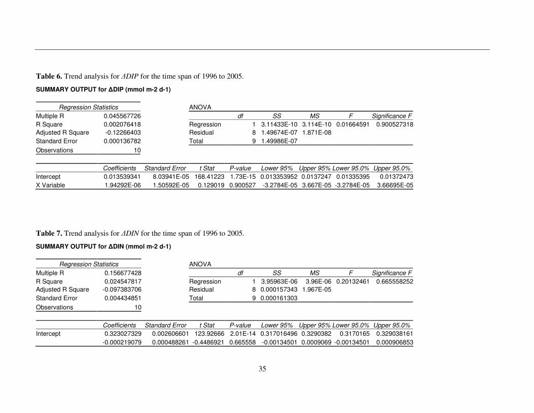
A closer visual look at the LOICZ budget results for phosphorous and nitrogen (e.g. Figure 9) do

not indicate any specific trend in order to possibly make a specific statement about if the water

quality and ecosystem functioning of the Mediterranean Sea are changing or remain stationary. A

more in-depth statistical analysis in this respect using linear regression to detect if trends could be

perceived for ∆DIP and ∆DIN for the time period 1996 to 2005 has been performed. The results

clearly show that the mean ∆DIP and ∆DIN values do not differ along different years for this

chosen time period (i.e., null hypothesis at the 95% confidence level cannot be reject and thus no

34

linear trend). Tables 6 and 7 show the results of this statistical analysis for ∆DIP and ∆DIN,

respectively.

The stoichiometric linkage of C, N and P through the Redfield ratio indicates that nitrogen fixation

and production of dissolved inorganic carbon dominate over denitrification and consumption of

dissolved inorganic carbon via net organic production.

35

Table 6. Trend analysis for ∆DIP for the time span of 1996 to 2005.

SUMMARY OUTPUT for ∆DIP (mmol m-2 d-1)

Regression Statistics ANOVA

Multiple R 0.045567726 df SS MS F Significance F

R Square 0.002076418 Regression 1 3.11433E-10 3.114E-10 0.01664591 0.900527318

Adjusted R Square -0.12266403 Residual 8 1.49674E-07 1.871E-08

Standard Error 0.000136782 Total 9 1.49986E-07

Observations 10

Coefficients Standard Error t Stat P-value Lower 95% Upper 95% Lower 95.0% Upper 95.0%

Intercept 0.013539341 8.03941E-05 168.41223 1.73E-15 0.013353952 0.0137247 0.01335395 0.01372473

X Variable 1.94292E-06 1.50592E-05 0.129019 0.900527 -3.2784E-05 3.667E-05 -3.2784E-05 3.66695E-05

Table 7. Trend analysis for ∆DIN for the time span of 1996 to 2005.

SUMMARY OUTPUT for ∆DIN (mmol m-2 d-1)

Regression Statistics ANOVA

Multiple R 0.156677428 df SS MS F Significance F

R Square 0.024547817 Regression 1 3.95963E-06 3.96E-06 0.20132461 0.665558252

Adjusted R Square -0.097383706 Residual 8 0.000157343 1.967E-05

Standard Error 0.004434851 Total 9 0.000161303

Observations 10

Coefficients Standard Error t Stat P-value Lower 95% Upper 95% Lower 95.0% Upper 95.0%

Intercept 0.323027329 0.002606601 123.92666 2.01E-14 0.317016496 0.3290382 0.3170165 0.329038161

-0.000219079 0.000488261 -0.4486921 0.665558 -0.00134501 0.0009069 -0.00134501 0.000906853

36

5. REFERENCES

Agostini, V.N. and A. Bakun. 2002. "Ocean Triads" in the Mediterranean Sea: Physical mechanisms potentially structuring reproductive habitat suitability (example application to European anchovy, Engraulis encrasicolus). Fisheries Oceanography 11:129-142.

Antonov, J. I., R. A. Locarnini, T. P. Boyer, A. V. Mishonov and H. E. Garcia. 2006. World Ocean

Atlas 2005, Volume 2: Salinity. S. Levitus, Ed. NOAA Atlas NESDIS 62, U.S. Government Printing Office, Washington, D.C., 182 pp.

Atkinson, M.J.and S.V. Smith. 1983. C:N:P ratios of benthic marine plants. Limnology and

Oceanography 28(3):568-574. Boyer, P., J.I. Antonov, H.E. Garcia, D.R. Johnson, R.A. Locarnini, A.V. Mishonov, M.T. Pitcher,

O.K. Baranova, I.V. Smolyar. 2006. World Ocean Database 2005. S. Levitus, Ed., NOAA Atlas NESDIS 60, U.S. Government Printing Office, Washington, D.C., 190 pp.

Bryden, H.L., J. Candela and T.H. Kinder. 1994. Exchange through the Strait of Gibraltar. Prog.

Oceanog. 33:201-248. EEA/UNEP. 1999. State and pressures of the marine and coastal Mediterranean Environment, EEA

Environmental assessment series N°5 Environmental indicators: Typology and overview, EEA Technical report No 25, http://reports.eea.europa.eu/medsea/en/medsea_en.pdf.

EEA. 2005. The European Environment State and Outlook 2005, State of Environment Report

No.1/2005.European Environment Agency, Copenhagen. 584pp. Evans, B.M., D.W. Lehning and K.J. Corradini. 2008. AVGWLF vers. 7.1, Users Guide, Penn State

Institutes of Energy and the Environment, The Pennsylvania State University, University Park, PA, 2008.

Garcia, H. E., R. A. Locarnini, T. P. Boyer and J. I. Antonov. 2006. World Ocean Atlas 2005,

Volume 4: Nutrients (phosphate, nitrate, silicate). S. Levitus, Ed. NOAA Atlas NESDIS 64, U.S. Government Printing Office, Washington, D.C., 396 pp.

Global Runoff Data Centre. 2008. River Discharge Data. Global Runoff Data Centre. Koblenz, Federal

Institute of Hydrology (BfG). Gordon, Jr., D. C., P. R. Boudreau, K. H. Mann, J.-E. Ong, W. L. Silvert, S. V. Smith, G.

Wattayakorn, F. Wulff and T. Yanagi. 1996. LOICZ Biogeochemical Modelling Guidelines, LOICZ Reports & Studies No 5, pp.1-96.

Haidvogel, D.B. and A. Beckmann. 2000. Numerical ocean circulation modeling. Imperial College

Press. 322pp. Holligan, P., de Boois, H. (eds.) 1993. Land-Ocean Interactions in the Coastal Zone: Science Plan.

IGBP Report No. 25. International Geosphere-Biosphere Programme, Stockholm. Hopkins, T.S. 1985. Physics of the Sea. In: Margalef, R. (Ed.). Western Mediterranean. Pergamon Press. Oxford. pp.100-125.

37

Hopkins, T.S. 1985. Physics of the sea. In: R. Margalef (ed.). Key Environments: Western Mediterranean. Pergamon Press. Oxford: 100-125.

Hopkins J.P. 1999. The thermohaline forcing of the Gibraltar exchange, J. Marine Systems, 20, 1–

31. Imberger, J., T. Berman, R. R. Christian, E. B. Sherr, D. E. Whitney, L. R. Pomeroy, R. G. Wiegert

and W. J. Wiebe. 1983. The Influence of Water Motion on the Distribution and Transport of Materials in a Salt Marsh Estuary. Limnology and Oceanography 28: 201-214.

Laubier, L. 2005. Mediterranean Sea and humans: Improving a conflictual partnership, In: The

Mediterranean Sea. Handbook of Environmental Chemistry. Ed.: Saliot, A, pp.3-27. Mariotti, A., M.V. Struglia, N. Zeng and K.-M. Lau. 2002. The hydrological cycle in the

Mediterranean region and implications for the water budget of the Mediterranean Sea, Journal of

Climate 15:1674–1690. Markaki, Z., M.D. Loÿe-Pilot, K. Violaki, L. Benyahya and N. Mihalopoulos. 2008. Variability of

atmospheric deposition of dissolved nitrogen and phosphorus in the Mediterranean and possible link to the anomalous seawater N/P ratio. Marine Chemistry. doi:10.1016/j.marchem.2008.10.005.

Peixoto, J. P., M. De Almeida, R. D. Rosen and D. A. Salstein. 1982. Atmospheric moisture

transport and the water balance of the Mediterranean Sea, Water Resour. Res. 18, 3–90. Pernetta, J.C. and Milliman, J.D. (eds) 1995. Land-Ocean Interactions in the Coastal Zone:

Implementation Plan. IGBP Global Change Report 33. IGBP, Stockholm, 215 pages. Pickard, G. L. and W. J. Emery. 1990. Descriptive Physical Oceanography: An Introduction, 5th ed., Pergamon Press, 320 pp. Povinec, P., Aggarwal, P., Aureli A., Burnett, W. C., Kontar, E. A., Kulkarni, K. M., Moore, W. S.,

Rajar, R., Taniguchi, M., Comanducci, J.-F., Cusimano, G., Dulaiova, H., Gatto, L., Hauser, S., Levy-Palomo, I., Ozorovich, Y. R., Privitera, A. M. G., Schiavo, M. A. 2006. Characterisation of submarine ground water discharge offshore south-eastern Sicily. Journal of Environmental

Radioactivity 89(1):81-101. Redfield, A. C. 1934. On the proportions of organic derivatives in seawater and their relation to the

composition of plankton. pp. 176-192 James Johnston Memorial Volume. (R. J. Daniel, ed.) University Press of Liverpool, Liverpool, England.

Simmons, A, S. Uppala, D. Dee and S. Kobayashi. 2007. ERA-Interim: New ECMWF reanalysis

products from 1989 onwards. ECMWF Newsletter 110. Somot, S., F. Sevault, and M. D´equ´e. 2006. Transient climate change scenario simulation of the

Mediterranean Sea for the 21st century using a high resolution ocean circulation model, Clim.

Dyn. 27(7-9):851–879. Strobl, R.O., F. Somma, B.M. Evans and J.M. Zaldívar. 2009. Fluxes of water and nutrients from

38

river runoff to the Mediterranean Sea using GIS and a watershed model. Journal of Geophysical Research: Oceanography. (in press)

Tomczak, M. and J.S. Godfrey. 2003. Regional Oceanography: An Introduction. 2nd Edition. Delhi, Daya Pub. ISBN 81-7035-307-6. Troccoli, A. and P. Kållberg. 2004. Precipitation correction in the ERA-40 reanalysis. ERA-40

project report series 13. ECMWF. Turk, F.J., P. Arkin, E.E. Ebert and M.R P Sapiano. 2008. Evaluating High-Resolution Precipitation

Products, Bulletin of the American Meteorological Society, Volume 89, pp.1911–1916. UNEP. 2003. Eutrophication monitoring strategy of MED POL. Mediterranean Action Plan, UNEP(DEC)/MED WG.231/14, 75 pp. UNEP/MAP/MED POL. 2004. Transboundary Diagnostic Analysis (TDA) for the Mediterranean

Sea, UNEP/MAP, Athens, 282 pp. Uppala, S.M. Kållberg, P. W., Simmons, A. J., Andrae, U., Bechtold, V. Da Costa, Fiorino, M.,

Gibson, J. K., Haseler, J., Hernandez, A., Kelly, G. A., Li, X., Onogi, K., Saarinen, S., Sokka, N., Allan, R. P., Andersson, E., Arpe, K., Balmaseda, M. A., Beljaars, A. C. M., Berg, L. Van De, Bidlot, J., Bormann, N., Caires, S., Chevallier, F., Dethof, A., Dragosavac, M., Fisher, M., Fuentes, M., Hagemann, S., Hólm, E., Hoskins, B. J., Isaksen, L., Janssen, P. A. E. M., Jenne, R., McNally, A. P., Mahfouf, J.-F., Morcrette, J.-J., Rayner, N. A., Saunders, R. W., Simon, P., Sterl, A., Trenberth, K. E., Untch, A., Vasiljevic, D., Viterbo, P., Woollen, J.2005. The ERA-40 re-analysis, Q. J. R. Meteorol. Soc. 131:2961-3012.

Webb, K.L. 1981. Conceptual models and processes of nutrient cycling in estuaries. In B.J. Neilson

and L.E. Cronin (Eds.). Estuaries and Nutrients. Humana, New Jersey. Pp.25-46. Zekster, I.S. and R.G. Dzhamalov. 1988. Role of ground water in the hydrologic cycle and in

continental water balance. UNESCO, Paris.

39

European Commission EUR 23936 EN – Joint Research Centre – Institute for Environment and Sustainability Title: Application of the LOICZ Methodology to the Mediterranean Sea Author(s): R.O. Strobl, J.M. Zaldívar Comenges, F. Somma, A. Stips and E. García Gorriz Luxembourg: Office for Official Publications of the European Communities 2009 – 41 pp. – 21 x 29,7 cm EUR – Scientific and Technical Research series – ISSN 1018-5593 ISBN 978-92-79-12794-6 DOI 10.2788/23549 Abstract

From a broad perspective, the LOICZ (Land-Ocean Interactions in the Coastal Zone) approach attempts to evaluate coastal change from a system perspective and assumes that the effects taking place are due to pressures within the whole basin. The LOICZ methodology was applied to the Mediterranean Sea in order to estimate its water, salt and nutrient budget, as well as to gain insights into its biogeochemical cycles. In order to undertake this budget approach, various input data relative to the three budgets were gathered for the time period of 1996 to 2005. In the case of the Mediterranean Sea, it was seen that there is still a gap between LOICZ data requirements and the standard monitoring practices in the coastal zone, both from a spatial as well as temporal viewpoint. The results show that on average over the time period 1996 to 2005, the phosphorous and nitrogen budgets of 1.35·10-2 mmol m-2 d-1 and 3.22·10-1 mmol m-2 d-1, respectively, suggest an excess of release over uptake. The budget calculations translate to the fact that on average the Mediterranean Sea acts as a sink of phosphorous and nitrogen. No specific, statistically relevant trend of the water quality and ecosystem functioning of the Mediterranean Sea was observed. An examination of the stoichiometric linkage of C, N and P through the Redfield ratio indicates that nitrogen fixation and production of dissolved inorganic carbon dominate over denitrification and consumption of dissolved inorganic carbon via net organic production.

40

How to obtain EU publications Our priced publications are available from EU Bookshop (http://bookshop.europa.eu), where you can place an order with the sales agent of your choice. The Publications Office has a worldwide network of sales agents. You can obtain their contact details by sending a fax to (352) 29 29-42758.

41

The mission of the JRC is to provide customer-driven scientific and technical support for the conception, development, implementation and monitoring of EU policies. As a service of the European Commission, the JRC functions as a reference centre of science and technology for the Union. Close to the policy-making process, it serves the common interest of the Member States, while being independent of special interests, whether private or national.

L

B- N

A- 2

393

6- E

N- C