Application of Viscous and Iwan Modal Damping Models to Experimental Measurements from Bolted Structures Brandon J. Deaner Structural Analyst Mercury Marine W6250 Pioneer Road P.O.Box 1939 Fond du Lac, WI 54936-1939 [email protected]Matthew S. Allen Associate Professor Department of Engineering Physics University of Wisconsin-Madison 535 Engineering Research Building 1500 Engineering Drive Madison, Wisconsin 53706 [email protected]Michael J. Starr Sandia National Laboratories P.O. Box 5800 Albuquerque, NM, 87185 [email protected]Daniel J. Segalman Research Scientist Department of Engineering Physics University of Wisconsin-Madison 538 Engineering Research Building 1500 Engineering Drive Madison, Wisconsin 53706 [email protected]Hartono Sumali Manager Science, Technology and Engineering Integration Sandia National Laboratories P.O. Box 5800 Albuquerque, NM, 87185 [email protected]ABSTRACT Measurements are presented from a two-beam structure with several bolted interfaces in order to characterize the nonlinear damping introduced by the joints. The measurements (all at force levels below macro-slip) reveal that each underlying mode of the structure is well approximated by a single degree-of-freedom system with a nonlinear mechanical joint. At low enough force levels the measurements show dissipation that scales as the second power of the applied force, agreeing with theory for a linear viscously damped system. This is attributed to linear viscous behavior of the material and/or damping provided by the support structure. At larger force levels the damping is observed to behave nonlinearly, suggesting that damping from the mechanical joints is dominant. A model is presented that captures these effects, consisting of a spring and viscous damping element in parallel with a 4- Parameter Iwan model. The parameters of this model are identified for each mode of the structure and comparisons suggest that the model captures the stiffness and damping accurately over a range of forcing levels.
Transcript
Application of Viscous and Iwan Modal Damping Models to Experimental
Measurements from Bolted Structures
Brandon J. Deaner Structural Analyst Mercury Marine
Measurements are presented from a two-beam structure with several bolted interfaces in order to characterize the nonlinear damping introduced by the joints. The measurements (all at force levels below macro-slip) reveal that each underlying mode of the structure is well approximated by a single degree-of-freedom system with a nonlinear mechanical joint. At low enough force levels the measurements show dissipation that scales as the second power of the applied force, agreeing with theory for a linear viscously damped system. This is attributed to linear viscous behavior of the material and/or damping provided by the support structure. At larger force levels the damping is observed to behave nonlinearly, suggesting that damping from the mechanical joints is dominant. A model is presented that captures these effects, consisting of a spring and viscous damping element in parallel with a 4-Parameter Iwan model. The parameters of this model are identified for each mode of the structure and comparisons suggest that the model captures the stiffness and damping accurately over a range of forcing levels.
Nomenclature FS Joint slip force Iwan parameter KT Joint stiffness Iwan parameter χ Power law energy dissipation Iwan parameter β Level of energy dissipation and curve of energy dissipation Iwan parameter K∞ Linear elastic stiffness of the system C Modal viscous damping coefficient q0 Modal amplitude of displacement ω Response frequency FLE Force in the linear elastic spring FIwan Force in the Iwan joint R Coefficient in the Iwan distribution function ϕmax Modal displacement at macro-slip FVD Force in the viscous damper Ftotal Total force in the modal Iwan model F J Force in the joint. DM Energy dissipated by the model KM Stiffness of the model fM Frequency of the model V(t) Analytic signal
( )v t Hilbert transform of the modal velocity ( )v t Modal velocity ψ(t) Decay Envelope ωn(t) Time varying natural frequency ζ(t) Time varying damping ratio ψi Phase angle KE Modal Kinetic Energy DE Energy dissipated by experimental data fE Frequency of the experimental data g Total optimization objective function gD Energy dissipation objective function gf Frequency objective function χinitial Power law energy dissipation Iwan parameter from graphical method
1. INTRODUCTION
Mechanical joints are known to be a major source of damping in assembled structures. However, the amplitude dependence of damping in mechanical joints has proven to be quite difficult to predict. For many systems, linear damping models seem to capture the response of a structure near the calibrated force level, but the damping may increase by an order of magnitude or more as the response level increases, leading to over-conservative designs. On the other hand, many of these structures still seem to exhibit the same uncoupled linear modes that were evident at low amplitudes. This work seeks to develop a model that is valid over a range of force levels and captures this variation in damping, while preserving much of the simplicity of the linear model.
Mechanical joints are said to be undergoing micro-slip when the joint as a whole remains intact but small slip displacements occur at the outskirts of the contact patch causing frictional energy loss in the system [1]. When this is the case the overall response of the structure is often well approximated with a linear model since the effective stiffness and mass do not change significantly, yet the change in the damping may be significant. The 4-Parameter Iwan model developed by Segalman [2] captures these effects and has been shown to reproduce the behavior of real lap joints as observed in an extensive testing and modeling campaign [1], including the power law energy dissipation seen in the micro-slip region. (Models of parallel arrangements of Jenkins elements have a long history; among those who have studied such models are Masing, Bauschinger, Prandtl, Ishlinskii, and Iwan [3].) In the past decade, the 4-Parameter Iwan model has been implemented to predict the vibration of structures with a few discrete joints [4, 5]. However, when modeling individual joints, each joint may require a unique set of parameters, which means that one must deduce hundreds or even thousands of joint parameters to describe a system of interest. On the other hand, when a small number of modes are active in a response, recent measurements have suggested that a simpler model may be adequate.
Segalman et al. recently applied the 4-Parameter Iwan model in a modal framework to describe both discrete joint simulations and experimental data from structures with bolted joints [6, 7]. While these efforts were motivated by empirical observations, the complexification and averaging method can be used to rigorously explain the conditions under which this type of model is appropriate [8]. In essence the natural frequencies of the system must be well separated and the nonlinearities small enough so that their primary effect is to modulate the response of each linear mode. While the work in [8] focused on presenting a general framework for structures with weak nonlinearities, this work focuses on a particular form for the model for each uncoupled oscillator (e.g. an SDOF modal Iwan model) and shows that it describes the system of interest exceedingly well. Furthermore, it was observed that at low force levels, the damping of the structure is dominated by material damping or other effects that are well approximated as linear, so a linear viscous damper was added in parallel with the 4-Parameter Iwan modal model to capture this effect.
It is worth noting that a system similar to the two beam structure used here was also studied by Gaul, Reuss et al. (see, e.g. [9, 10]), and an excellent review of their work on joint modeling was presented by Bograd, Reuss et al. in [11]. Their review discusses a range of approaches from zero thickness elements that can be added to the FE model to capture the joint behavior in detail to whole joint models such as the Iwan model mentioned earlier, and it discusses how the harmonic balance method can be used to model the nonlinear behavior of the joint. They conclude that the “dominant limiting factor in joint modeling to date is probably the long simulation times associated with many of the joint models as well as uncertainty associated with joint parameter estimation.” This work seeks to contribute on these two fronts, first by exploring a model form that can be simulated very inexpensively and by evaluating its utility in representing real measurements. It is hoped that this model could eventually serve as an intermediary between expensive, high fidelity, predictive simulations such as those described in [11-13] and experimental measurements. This work also focuses particularly on experimental methods that allow one to evaluate whether this model can capture the nonlinear dependence of damping over a range of response amplitude, as was done rigorously by Segalman et al. [14] with regard to the discrete Iwan model.
The following sections review the modal Iwan modeling framework proposed by Segalman and discuss an experimental approach that can be used to deduce the modal Iwan parameters from measurements. These ideas are then applied to an assembly of two beams that are joined by four lap joints and the identified model is found to reproduce the behavior of the first several modes quite adequately.
1.1 Modal Model
Segalman proposed that nonlinear energy dissipation due to bolted joints could be applied on a mode-by-mode basis, using a 4-parameter Iwan constitutive model for each mode [6]. In general, the nonlinearity that joints introduce can couple the modes of a system so that modes in the traditional linear sense can not be defined. However, damping is often a relatively weak effect and experiments have shown that the modes of structures with joints are typically quite linear and uncoupled. This suggests that one might be able to model the structure as a collection of uncoupled linear modes, each with nonlinear damping characteristics [7], and this is precisely the approach adopted in this work.
Indeed, consider the rth mode of a structure with weak joint nonlinearities. Its equation of motion can be written as
21 2, ,... ( )r r r r r r r I r extq q q f q q f t T Tφ φ (1)
where r and r are the modal natural frequency and damping ratio of the linear part of the system (e.g. at small amplitude), fI denotes the nonlinear force due to the joints, and fext the external forces. Eriten et al. [8] used the complexification to explain how weak nonlinear forces, fI, cause the frequency and damping of the oscillator to vary slightly while the response remains mono-harmonic. Under these assumptions, each modal degree-of-freedom will be modeled by a single degree-of-freedom oscillator, as shown in
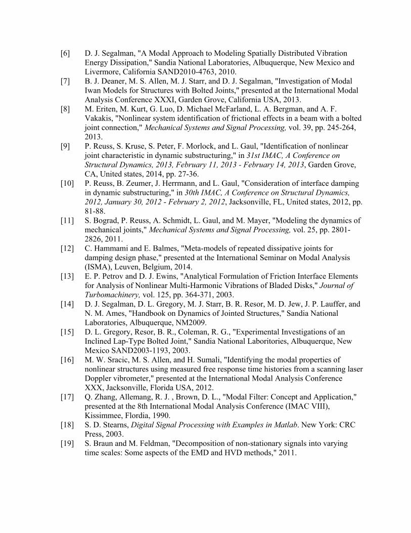
Fig. 1, with a 4-parameter Iwan model in parallel with a viscous damper and an elastic spring. Note that the displacement of the mass is not a physical displacement but the modal displacement or modal amplitude, q, of the mode of interest. The mode vectors are mass normalized so the modal mass is taken to be unity. Fig. 1 about here The 4-parameter Iwan model has parameters {FS, KT, χ, β} where FS is the joint force necessary to initiate macro-slip, KT is the stiffness of the joint, χ is directly related to the slope of the damping of the system versus amplitude in the micro-slip regime, and β relates to the level of energy dissipation and the shape of the energy dissipation curve as the macro-slip force is approached. Finally, the viscous damper has a coefficient, C, and the linear elastic spring stiffness is K∞. The viscous damper accounts for the linear damping associated with the material and the boundary conditions. If a structure truly has only material damping, then one could determine an equivalent modal damping coefficient, C, for each mode from the material’s loss factor. In other applications C can simply be fit from measurements to account for the linear part of all damping mechanisms present (e.g. acoustic, due to energy dissipated or waves carried away by the support structure, etc…). Note that all of the parameters are defined in modal and not physical space.
2. Analytical Models for Energy Dissipation and Frequency The energy dissipation for the modal model seen in
Fig. 1 can be found analytically and used to fit experimental data. Assuming a harmonic load is applied to the mass and the system is at steady-state, the mass will oscillate as
0 sin( )q q t (2)
where q0 is the modal displacement amplitude and ω is the response frequency. The force in the linear elastic spring takes the form
LEF K q (3)
where K∞ is the spring stiffness. The force in the Iwan joint is given in [2] for an arbitrary loading. Assuming that the amplitude of motion is small, 0 maxq or in other words the
Iwan joint is undergoing micro-slip, in [2] Segalman showed that the force in the Iwan model can be approximated as
2
2Iwan
RqF
(4)
where R is a coefficient that describes the population distribution of the parallel-series Iwan system [2]. The modal Iwan parameter R can be written in terms of the joint parameters as
2max
1
12
SFR
(5)
where
max
1
12
S
T
F
K
(6)
Finally, the force in the viscous damper can be written as
VDF Cq (7)
where C is the viscous damping coefficient. These forces can be added, for each modal joint model so that
Total VD LE IwanF F F F for the model in
Fig. 1. The total forces are then multiplied by the modal velocity and integrated over one period as follows,
2
0M TotalD F q dt (8)
to obtain the energy dissipated per cycle, DM. The energy dissipation in the micro-slip regime for this model is
3200
4
3 2Micro
RqD Cq
(9)
Notice that the energy dissipation depends on the maximum modal amplitude q0 and that, as expected, the linear elastic spring does not contribute to the energy dissipated.
In the macro-slip region, the force in the Iwan joint has saturated and hence
Iwan SF F . Therefore, the modal energy dissipation is given by the following.
20 04Macro SD q F Cq (10)
Therefore, the total energy dissipation can be written as:
max
max
if or
if or
JMicro S
M JMacro S
D F F qD
D F F q
(11)
where JF is the force in the joint. The secant stiffness of the Iwan joint in the micro-slip region can be approximated as [2]
1
12 1Micro T
rK K K
(12)
where
0
12
1
T
S
q K
rF
(13)
In the macro-slip region, the stiffness is given by:
MacroK K (14)
Therefore, the stiffness of the joint can be written as follows.
, max
, max
if or
if or
JMicro r S
M JMacro r S
K F F qK
K F F q
(15)
Assuming mass normalized mode shapes are used, the natural frequency of the analytical model is then
2
MM
Kf
(16)
Note that these expressions are only approximations to the actual dissipation and frequency. In order to obtain the actual energy dissipation and instantaneous natural frequency, the Iwan model can be integrated in time and then the actual dissipation and frequency can be deduced. However, as discussed in a later section, these expressions for DM and fM are useful as they are very inexpensive to compute, and hence they will be used in an optimization problem to find the modal Iwan parameters that best fit the data.
3. Processing Transient Excitation Measurements
The energy dissipation for each mode of a system can be computed from measurements of its free response. Various methods for calculating the frequency and energy dissipation
have been used in previous works [7, 15, 16]. The procedure used to process measurements in this work is introduced below.
3.1 Single Degree-of-Freedom Response Model
First, a filter is used to isolate the modal response of the rth mode, which is denoted ( )rq t . The authors have used both modal filters [17] and standard, infinite impulse response
band-pass filters [18] for this purpose and other possibilities certainly exist. In their pioneering efforts Eriten et al. [8] used Empirical Mode Decomposition although EMD can become difficult if the signals to be separated have widely varying amplitudes or close frequencies [19] and in any event it is far more challenging than the aforementioned alternatives. While both band-pass filtering and EMD will fail if the system of interest contains modes with similar natural frequencies, one should recall that in that case there is not necessarily any theoretical basis for assuming that the two modes will remain uncoupled even if the nonlinearity is weak so a more complicated model might be needed; such a case is not considered in this work.
Once a single mode has been isolated, its response will be assumed to have the following form
0( ) Re exp ( ) exp i ( )v t A t t (17)
or
0( ) Re exp ( )
( ) ( ) i ( )r i
v t A t
t t t
(18)
where ( ) ( )rv t q t is the modal velocity for the mode of interest and Re{} denotes the real
part of a complex quantity. Then ( ) 0r t t describes the damping of the harmonic and
( )i t , describes the instantaneous frequency. The Hilbert transform is used to fit the
response model to the measured modal response. This work uses a variant [20] where a polynomial is fit to smooth the instantaneous amplitude and phase found by a standard Hilbert transform and then the curve fit model can be differentiated to estimate the instantaneous frequency, as explained below.
Given a sampled representation of the velocity signal, ( )v t , a sampled representation of the analytic signal, denoted ( )V t , can be found by adding the Hilbert transform of the modal velocity, ( )v t , as follows
( ) ( ) ( )V t v t iv t (19)
Then ( )t can be obtained using
0
10
exp ( ) ( )
( )( ) arg arg ( ) tan
( )
r
i
A t V t
v tt A V t
v t
(20)
Now the instantaneous frequency is defined to be the derivative of the phase,
( ) id
dt
dt
(21)
which produces the expected result for a linear response (see, Feldman [21], Sec. 3.2). The same is done for the decay envelope using the following definition.
( ) rddt
dt dt
(22)
One can then proceed to define the time-varying damping ratio and natural frequency using the following, which also gives the expected result for a linear time invariant system.
( ) ( ) ( )nt t t (23)
Combining these equations with the following
2( ) ( ) 1 ( )d nt t t (24)
one can establish unique values for the time varying natural frequency, damped natural frequency and damping ratio of the nonlinear system. It is important to note that these are merely parameters that describe the response of the nonlinear system; they are not readily connected to the equation of motion for the system.
3.2 Relationship to Linear Systems
For a linear system, ( )r nt t and ( )i dt t and the natural frequency and
damping ratio are also readily related to the linear system’s equation of motion, which is the following.
22 0n nx x x (25)
On the other hand, it is not so straightforward to relate the response model to the equation of motion of the nonlinear system. For example, suppose that a system has the following equation of motion, which is essentially the equation of motion above with the natural frequency and damping ratio replaced by their time varying counterparts.
22 ( ) ( ) ( ) 0n nx t t x t x (26)
If the trial solution 0( ) Re exp ( )x t A t is inserted into the equation of motion above and
the definitions in Eq. (21) through (23) are used, one finds that the differential equation is NOT satisfied. The residual is given below and one can see that it is not generally zero unless and n are both constant.
( ) ( )( )
( ) ( ) i 0n dn
d t d td tt t
dt dt dt
(27)
As mentioned previously, the complexification approach discussed in [8] and [22] can be used to compute the time varying amplitude and frequency of a nonlinear system from its equation of motion, allowing one to estimate a response model of this form directly from the equation of motion. The approach is similar to that which was used in Sec. 2 to derive the expression for energy dissipation versus amplitude for the Iwan model.
3.3 Reducing Noise in Hilbert Transform
The derivatives required in Eqs. (21) and (22) are highly problematic for measured data. In his work, Feldman uses a filter to smooth the signals ( )r t and ( )i t that are obtained
from measurements. However, apparently due to intellectual property restrictions, his
publications do not explain his algorithm in detail. In this work we take the approach that was first suggested by Sumali et al. in [20], and curve fit the measurements to polynomials to minimize noise. Specifically, a polynomial of degree, p is fit to the phase signal ( )i t . Prior
to fitting the data, the beginning and end of the time record are deleted as they tend to be contaminated due to the end effects of the Hilbert Transform algorithm. The time indices that are used are denoted 0 1 1, , , Nt t t , where N is less than the length of the original time
series due to the samples that have been truncated.
0 0 0
1 1 1
1
1 01 1
( ) 1
( ) 1
1
( ) 1
pi p
pi
pi N N N
t bt t
t t t
b
t bt t
(28)
The polynomial coefficients b0, b1, ..., bp can be obtained by a least squares solution of the above system of equations and then it is straightforward to differentiate the model in Eq. (28) to obtain the derivatives in Eqs. (21) and (22). It should be noted that in general it is important to normalize t so that the maximum value is one, otherwise the equations become numerically ill-conditioned and serious errors can result. The amplitude of the analytic signal is also fit to a polynomial resulting in a model for ( )V t , which is related to ( )r t .
Now the energy dissipation per cycle can be calculated from the change in kinetic energy over one cycle. The amplitude of the kinetic energy can be written as,
2
0
1exp ( )
2 rKE M A t (29)
where M is assumed to be unity since the mode shapes are mass normalized. The change in the kinetic energy is found by taking the derivative of this expression. Since the kinetic energy and its derivative are quite smooth, the energy dissipated per cycle, DE, can be approximated by simply multiplying dKE/dt by the period (2/n(t)) (e.g. using a trapezoid rule to integrate the power dissipated as a function of time).
2 4
( )En n
dKED t KE
dt
(30)
Finally, the time varying natural frequency is converted from radians per second to Hertz and is denoted as the experimental modal frequency.
( )
2n
E
tf
(31)
In order to relate DE to the analytical expression for the energy dissipation, in Eq. (9), the displacement amplitude is needed as a function of time. This was obtained by integrating the measured velocity signal ( )v t with respect to time using a trapezoidal numerical integration and assuming that the resulting displacement signal had zero mean. The Hilbert Transform analysis described above was then used to calculate the displacement amplitude as a function of time.
4. Parameter Identification
After the data has been filtered the parameters {FS, KT, K∞, χ, β} need to be identified for each mode. The parameters, {FS, KT, K∞, χ, β}, of the modal Iwan model can be found using a graphical approach as described in [7]. First, the experimental energy dissipated per cycle, DE, and stiffness, fE, are obtained using the procedure described in the previous section. The energy dissipation per cycle and stiffness can then be plotted versus the modal acceleration q , and since the mode shapes are mass normalized this is equal to the modal force.
The χinital parameter is found by fitting a line to the data for the log of energy dissipation versus log of the modal force at low force levels. Then the χinitial parameter for each mode r is given by:
, Slope 3initial r r (32)
In order to deduce the modal Iwan stiffness, KT, the natural frequencies of each mode are plotted versus modal joint force. A softening of the system, characterized by a drop in frequency, illustrates the amount of modal stiffness associated with all the relevant joints of the system. The equation for modal joint stiffness for each mode becomes
2 2, 0, , 0, ,T r r r r rK K K (33)
where ω0 is the natural frequency corresponding to the case when all the joints in the structure exhibit no slipping, and ω∞ is the natural frequency when all of the joints are slipping. However, macro-slip was not clearly observed at the force levels tested so ω∞ values were simply assumed to be slightly lower than the lowest observed natural frequency.
The modal joint slip force, FS, can be estimated from the modal force level at which the stiffness or natural frequency begins to drop. To find the last parameter, β, all of the previous parameters found are needed along with the y-intercept, Ar, of the line that was fit in order to find χinitial,r. Then, the following equation from [2] can be used to solve for r numerically.
11 1
2,
, 23,
14 1
2
2 3 1
r r
r
rr
rr T r r
rS r
r r r r r
K
FA K
(34)
While this graphical approach is convenient and lends significant insight into the meaning of each parameter, in this work that approach was used only to get initial guesses for the parameters which were then refined using an optimization routine. The modal Iwan parameters {FS, KT, K∞, χ, β, C} of the model in
Fig. 1, were fit to experimental data using several different optimization routines. The objective function was posed as:
Min g D fg g (35)
where
2
maxE M
DE M
D Dg
D D
(36)
and
2
maxE M
fE M
f fg
f f
(37)
Note that the dissipation and stiffness objective functions, gD and gf respectively, are weighted so that their values are on the same order of magnitude, and this has proved sufficient to obtain a well conditioned optimization problem in the applications studied to date.
The nonlinear objective function, Eq. (35), can be optimized using either local or global optimization. Both techniques were explored by the authors in this work; however, the objective functions here have multiple local minima, so the local optimization algorithms tended to be highly dependent on the starting guess. Therefore, a global optimization algorithm (the DIRECT algorithm developed by Jones et al. [23]) was found to be more robust. In addition, local optimization routines were used in MATLAB (fminsearch, fmincon, lsqnonlin [24]) to fine tune the solution and ensure convergence. Even with the global optimization algorithm, it was important to have a reasonable starting guess. For this work, starting guesses for the {FS, KT, K∞, χ, β} parameters were found using the graphical approach described previously. The initial guess for the modal viscous damping parameter, C, was obtained using an approximate modal damping ratio with C = 2mζω0.
5. Experiments on Two-Beam Structure
The proposed damping model was assessed using experimental measurements on a structure comprised of two beams bolted together. The structure was tested in free-free conditions, and care was taken to design the experimental setup to minimize the effect of damping associated with the boundary conditions. Free boundary conditions were used because any other choice, e.g. clamped, would add even more damping to the system.
5.1 Test Structure
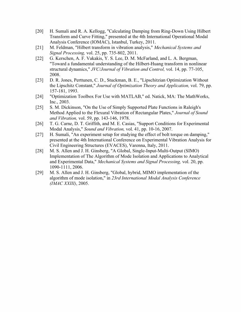
In this work, the structure consisted of two beams bolted together with four bolts as shown in Fig. 2. The two beams, each with dimensions 508 mm 50.8 mm 6.35 mm (20" 2" 0.25") were fastened together with 1/4"-28 fine-threaded bolts and all components were made of AISI 304 stainless steel. The bolts were tightened to three different torque levels in these tests: 1.13, 3.39, 5.65 N-m (10, 30, and 50 in-lbs). For reference, the Society of Automotive Engineers (SAE) provides the general torque specification for this type of bolt to be approximately 8.5 N-m (75.0 in-lbs) [25] which results in bolt preload force of approximately 6700 N (1500 lbf). The largest torque used here was somewhat lower than this specification, but, as will be shown, this structure became quite linear for the range of excitation forces that were practical with this setup, so the bolts were kept somewhat loose to accentuate the nonlinearity. Future works will explore methods of exciting the structure with higher force levels (closer to what might be seen in the applications of interest) so that more realistic torques can be used.
Fig. 2 about here
5.2 Experimental Setup
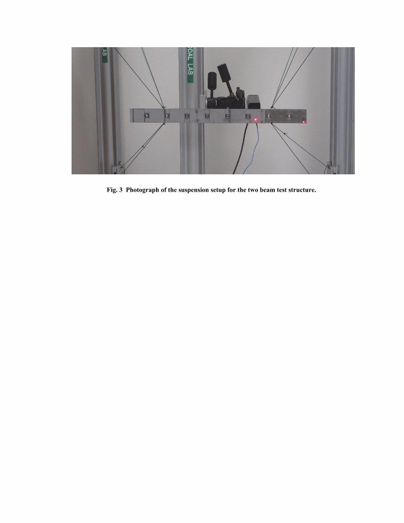
The dynamic response of the two beam structure was captured using a scanning laser Doppler vibrometer (Polytec PSV-400), which measured the response at 70 points on the structure. In addition, a single point laser vibrometer (Polytec OFV-534) was used to measure at a reference point to verify that the hammer hits were consistent. The reference laser was positioned close to the impact force location as seen in Fig. 2.
Fig. 3 about here
The structure was suspended by 2 strings that support the weight of the structure and 8 bungee cords which prevent excessive rigid-body motion. The bungees and strings were connected to the beam at locations where the odd bending modes have little motion in order to minimize the damping added to the system for these modes.
An Alta Solutions automated impact hammer with a nylon hammer tip was used to supply the impact force, which is measured by a force gauge attached between the hammer and the hammer tip. Additional measurements were taken at higher force levels using a modal hammer; however, the supplied impact force was not as consistent. The mean and standard deviation of the maximum impact force for all of the torque levels and force levels that were used in this study are shown in Table 1.
Table 1: Mean and standard deviation of the maximum impact force for all 70 measurements.
The automatic hammer provided a range of force levels between approximately 20 and
300 N. However, the force level depends on the distance between the hammer tip and the beam and the voltage supplied to the automatic hammer. For these reasons, the lowest and highest force varied for each measurement. For the automatic hammer, the standard deviation tended to increase as the force level increased. At the highest force level, the automatic hammer had a large spread for all the torque levels especially the 3.39 N-m torque. The modal hammer was able to achieve much higher force levels (approximately 1400 N);
however, it was much less consistent than the automatic hammer as illustrated by the large standard deviation in its impact force.
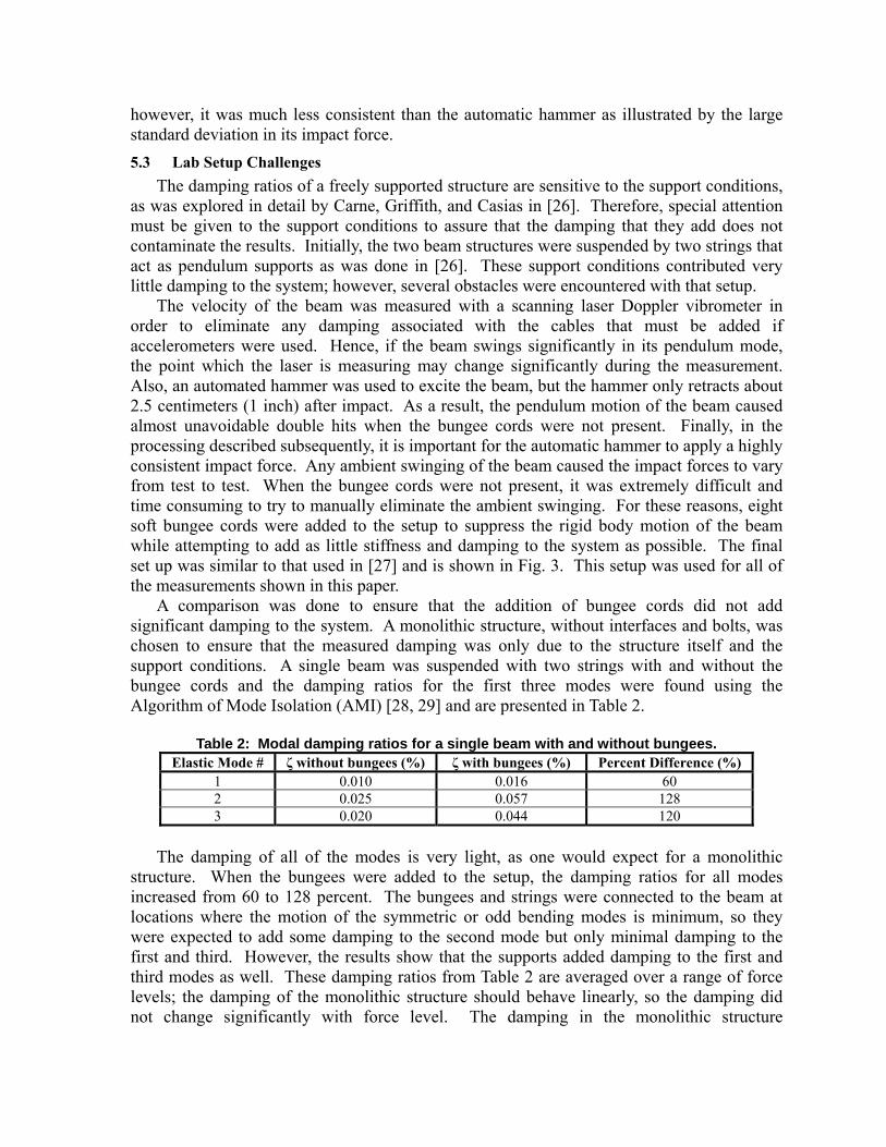
5.3 Lab Setup Challenges
The damping ratios of a freely supported structure are sensitive to the support conditions, as was explored in detail by Carne, Griffith, and Casias in [26]. Therefore, special attention must be given to the support conditions to assure that the damping that they add does not contaminate the results. Initially, the two beam structures were suspended by two strings that act as pendulum supports as was done in [26]. These support conditions contributed very little damping to the system; however, several obstacles were encountered with that setup.
The velocity of the beam was measured with a scanning laser Doppler vibrometer in order to eliminate any damping associated with the cables that must be added if accelerometers were used. Hence, if the beam swings significantly in its pendulum mode, the point which the laser is measuring may change significantly during the measurement. Also, an automated hammer was used to excite the beam, but the hammer only retracts about 2.5 centimeters (1 inch) after impact. As a result, the pendulum motion of the beam caused almost unavoidable double hits when the bungee cords were not present. Finally, in the processing described subsequently, it is important for the automatic hammer to apply a highly consistent impact force. Any ambient swinging of the beam caused the impact forces to vary from test to test. When the bungee cords were not present, it was extremely difficult and time consuming to try to manually eliminate the ambient swinging. For these reasons, eight soft bungee cords were added to the setup to suppress the rigid body motion of the beam while attempting to add as little stiffness and damping to the system as possible. The final set up was similar to that used in [27] and is shown in Fig. 3. This setup was used for all of the measurements shown in this paper.
A comparison was done to ensure that the addition of bungee cords did not add significant damping to the system. A monolithic structure, without interfaces and bolts, was chosen to ensure that the measured damping was only due to the structure itself and the support conditions. A single beam was suspended with two strings with and without the bungee cords and the damping ratios for the first three modes were found using the Algorithm of Mode Isolation (AMI) [28, 29] and are presented in Table 2.
Table 2: Modal damping ratios for a single beam with and without bungees.
The damping of all of the modes is very light, as one would expect for a monolithic
structure. When the bungees were added to the setup, the damping ratios for all modes increased from 60 to 128 percent. The bungees and strings were connected to the beam at locations where the motion of the symmetric or odd bending modes is minimum, so they were expected to add some damping to the second mode but only minimal damping to the first and third. However, the results show that the supports added damping to the first and third modes as well. These damping ratios from Table 2 are averaged over a range of force levels; the damping of the monolithic structure should behave linearly, so the damping did not change significantly with force level. The damping in the monolithic structure
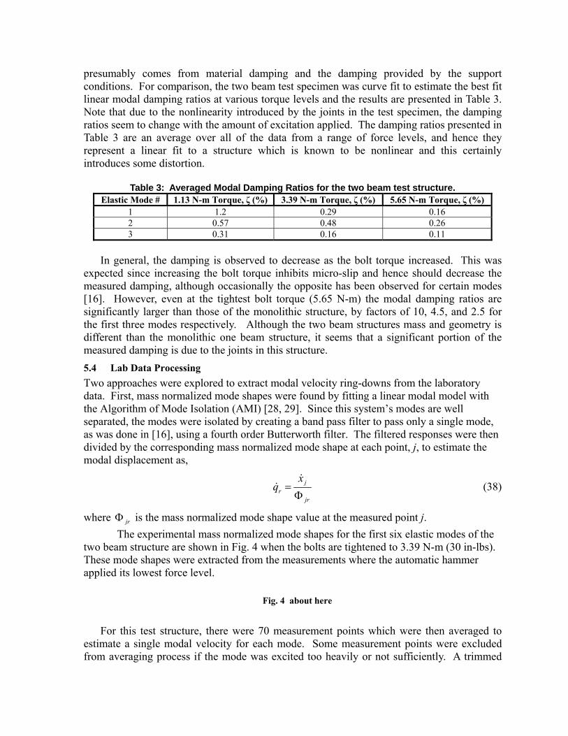
presumably comes from material damping and the damping provided by the support conditions. For comparison, the two beam test specimen was curve fit to estimate the best fit linear modal damping ratios at various torque levels and the results are presented in Table 3. Note that due to the nonlinearity introduced by the joints in the test specimen, the damping ratios seem to change with the amount of excitation applied. The damping ratios presented in Table 3 are an average over all of the data from a range of force levels, and hence they represent a linear fit to a structure which is known to be nonlinear and this certainly introduces some distortion.
Table 3: Averaged Modal Damping Ratios for the two beam test structure.
In general, the damping is observed to decrease as the bolt torque increased. This was
expected since increasing the bolt torque inhibits micro-slip and hence should decrease the measured damping, although occasionally the opposite has been observed for certain modes [16]. However, even at the tightest bolt torque (5.65 N-m) the modal damping ratios are significantly larger than those of the monolithic structure, by factors of 10, 4.5, and 2.5 for the first three modes respectively. Although the two beam structures mass and geometry is different than the monolithic one beam structure, it seems that a significant portion of the measured damping is due to the joints in this structure.
5.4 Lab Data Processing
Two approaches were explored to extract modal velocity ring-downs from the laboratory data. First, mass normalized mode shapes were found by fitting a linear modal model with the Algorithm of Mode Isolation (AMI) [28, 29]. Since this system’s modes are well separated, the modes were isolated by creating a band pass filter to pass only a single mode, as was done in [16], using a fourth order Butterworth filter. The filtered responses were then divided by the corresponding mass normalized mode shape at each point, j, to estimate the modal displacement as,
jr
jr
xq
(38)
where jr is the mass normalized mode shape value at the measured point j.
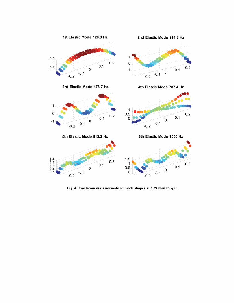
The experimental mass normalized mode shapes for the first six elastic modes of the two beam structure are shown in Fig. 4 when the bolts are tightened to 3.39 N-m (30 in-lbs). These mode shapes were extracted from the measurements where the automatic hammer applied its lowest force level.
Fig. 4 about here
For this test structure, there were 70 measurement points which were then averaged to
estimate a single modal velocity for each mode. Some measurement points were excluded from averaging process if the mode was excited too heavily or not sufficiently. A trimmed
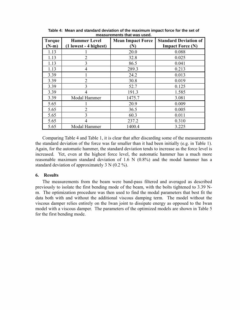
mean was used to determine which measurements to keep. The trimmed mean procedure excluded 8 high and low outliers from the set of 70 measurements points. All measurement points whose maximum velocity was within 50 percent of the trimmed mean were kept. The resulting statistics on the filtered impact hammer data are presented in Table 4.
Table 4: Mean and standard deviation of the maximum impact force for the set of measurements that was used.
Comparing Table 4 and Table 1, it is clear that after discarding some of the measurements
the standard deviation of the force was far smaller than it had been initially (e.g. in Table 1). Again, for the automatic hammer, the standard deviation tends to increase as the force level is increased. Yet, even at the highest force level, the automatic hammer has a much more reasonable maximum standard deviation of 1.6 N (0.8%) and the modal hammer has a standard deviation of approximately 3 N (0.2 %).
6. Results
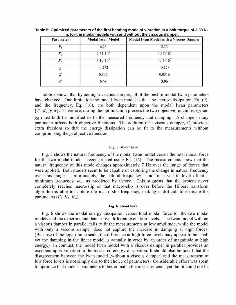
The measurements from the beam were band-pass filtered and averaged as described previously to isolate the first bending mode of the beam, with the bolts tightened to 3.39 N-m. The optimization procedure was then used to find the modal parameters that best fit the data both with and without the additional viscous damping term. The model without the viscous damper relies entirely on the Iwan joint to dissipate energy as opposed to the Iwan model with a viscous damper. The parameters of the optimized models are shown in Table 5 for the first bending mode.
Table 5: Optimized parameters of the first bending mode of vibration at a bolt torque of 3.39 N-m, for the modal models with and without the viscous damper.
Parameter Modal Iwan Model Modal Iwan Model with a Viscous Damper
FS 6.23 2.33
KT 2.61·105 1.37·105
K∞ 3.19·105 4.41·105
χ -0.272 -0.178
β 0.836 0.0316
C N/A 3.96
Table 5 shows that by adding a viscous damper, all of the best fit modal Iwan parameters
have changed. One limitation the modal Iwan model is that the energy dissipation, Eq. (9), and the frequency, Eq. (16), are both dependent upon the modal Iwan parameters , , ,S TF K . Therefore, during the optimization process the two objective functions, gD and
gf, must both be modified to fit the measured frequency and damping. A change in any parameter affects both objective functions. The addition of a viscous damper, C, provides extra freedom so that the energy dissipation can be fit to the measurements without compromising the gf objective function.
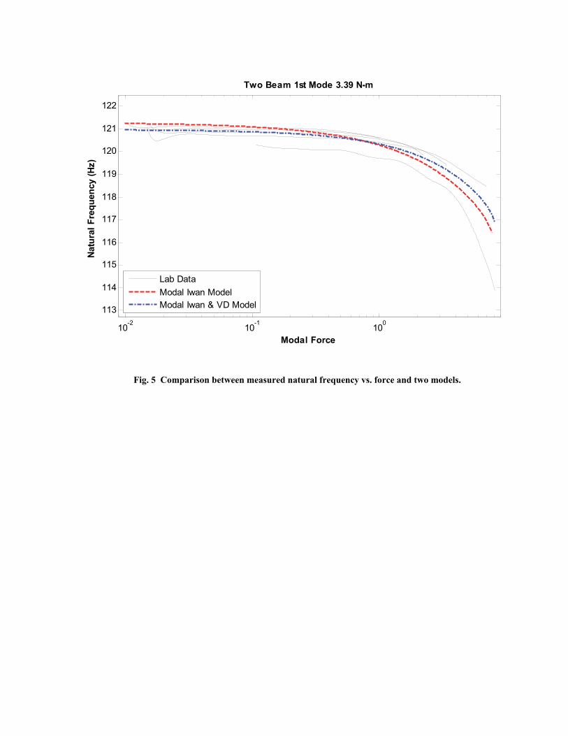
Fig. 5 about here
Fig. 5 shows the natural frequency of the modal Iwan model versus the total modal force for the two modal models, reconstructed using Eq. (16). The measurements show that the natural frequency of this mode changes approximately 7 Hz over the range of forces that were applied. Both models seem to be capable of capturing the change in natural frequency over this range. Unfortunately, the natural frequency is not observed to level off at a minimum frequency, ω∞, as predicted by theory. This suggests that the system never completely reaches macro-slip or that macro-slip is over before the Hilbert transform algorithm is able to capture the macro-slip frequency, making it difficult to estimate the parameters (FS, KT, K∞).
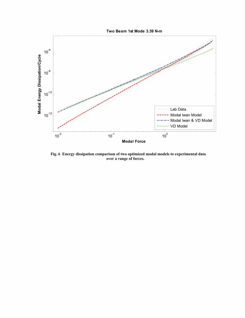
Fig. 6 about here.
Fig. 6 shows the modal energy dissipation versus total modal force for the two modal models and the experimental data at five different excitation levels. The Iwan model without a viscous damper in parallel fails to fit the measurements at low amplitude, while the model with only a viscous damper does not capture the increase in damping at high forces. (Because of the logarithmic scale, the difference at high force levels may appear to be small yet the damping in the linear model is actually in error by an order of magnitude at high energy.) In contrast, the modal Iwan model with a viscous damper in parallel provides an excellent approximation to the measured energy dissipation. It should also be noted that the disagreement between the Iwan model (without a viscous damper) and the measurement at low force levels is not simply due to the choice of parameters. Considerable effort was spent to optimize that model's parameters to better match the measurements, yet the fit could not be
improved without decreasing the agreement of the natural frequency versus force plot in Fig. 5. This difficulty disappeared when a viscous damper was added to the model.
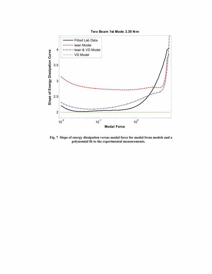
The differences between these models is more easily visualized by comparing the slope of the energy dissipation versus force curve. As mentioned previously, a single Iwan joint exhibits a slope of 3+ on a log dissipation versus log force plot. Fig. 7 compares the slope of the two optimized modal models with the experimentally measured slope. A fifth order polynomial was fit to the laboratory data in order to compute its slope. Without an additional viscous damper, the modal Iwan model has a much larger slope than the laboratory data at low force levels. On the other hand, when a viscous damper is added in parallel with the Iwan joint, the slope follows the laboratory data more closely over the entire range of force levels.
Note that the optimized models have identified a value for the slip force, FS, that is in the range of the measured forces. This suggests that macro-slip was initiated at the highest measured force levels. Unfortunately, the exciter that was used was not capable of exerting even higher forces so macro-slip could not be fully characterized.
Fig. 7 about here.
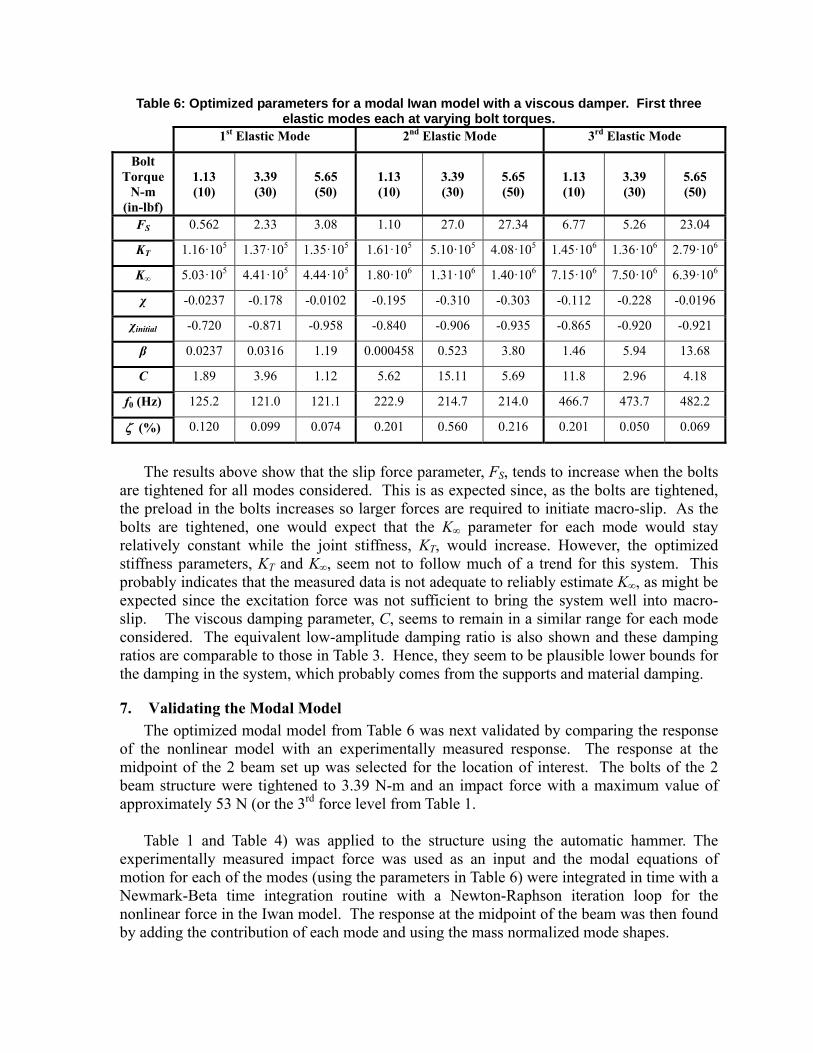
This same procedure was repeated for the first three elastic modes at three different bolt torques and the identified modal Iwan parameters are shown in Table 6. Only the first three elastic modes were analyzed in this work because a soft hammer tip was used which caused the higher frequency modes to respond quite weakly in these measurements. The last two rows of each section in Table 6 give the natural frequency and modal damping ratio of the mode at low force levels, both of which are readily computed from the other parameters.
Table 6: Optimized parameters for a modal Iwan model with a viscous damper. First three elastic modes each at varying bolt torques.
The results above show that the slip force parameter, FS, tends to increase when the bolts
are tightened for all modes considered. This is as expected since, as the bolts are tightened, the preload in the bolts increases so larger forces are required to initiate macro-slip. As the bolts are tightened, one would expect that the K∞ parameter for each mode would stay relatively constant while the joint stiffness, KT, would increase. However, the optimized stiffness parameters, KT and K∞, seem not to follow much of a trend for this system. This probably indicates that the measured data is not adequate to reliably estimate K∞, as might be expected since the excitation force was not sufficient to bring the system well into macro-slip. The viscous damping parameter, C, seems to remain in a similar range for each mode considered. The equivalent low-amplitude damping ratio is also shown and these damping ratios are comparable to those in Table 3. Hence, they seem to be plausible lower bounds for the damping in the system, which probably comes from the supports and material damping.
7. Validating the Modal Model
The optimized modal model from Table 6 was next validated by comparing the response of the nonlinear model with an experimentally measured response. The response at the midpoint of the 2 beam set up was selected for the location of interest. The bolts of the 2 beam structure were tightened to 3.39 N-m and an impact force with a maximum value of approximately 53 N (or the 3rd force level from Table 1.
Table 1 and Table 4) was applied to the structure using the automatic hammer. The
experimentally measured impact force was used as an input and the modal equations of motion for each of the modes (using the parameters in Table 6) were integrated in time with a Newmark-Beta time integration routine with a Newton-Raphson iteration loop for the nonlinear force in the Iwan model. The response at the midpoint of the beam was then found by adding the contribution of each mode and using the mass normalized mode shapes.
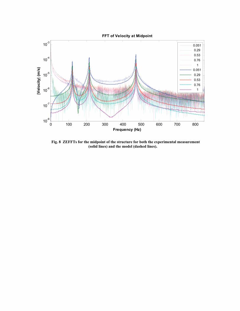
The responses were first compared in the frequency domain where it was easy to ignore the effect of the rigid body modes. A zeroed early-time fast Fourier transform (ZEFFT) [4] was used to show how the nonlinearity of both the model and the measured data progressed over time. Fig. 8 shows the ZEFFTs taken at several different times including: 0.051, 0.29, 0.53, 0.76, and 1.0 seconds as indicated in the legend. The solid and dashed lines correspond to the experimentally measured response and the simulated response from the three uncoupled modal Iwan models respectively.
Fig. 8 about here.
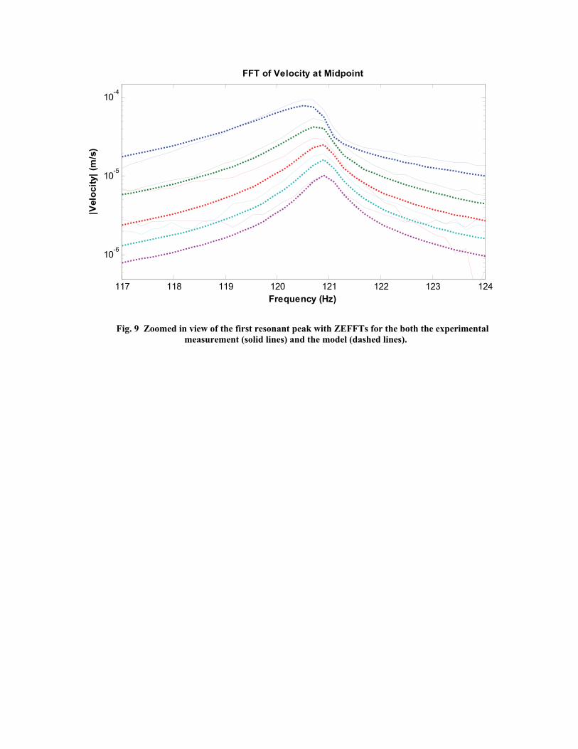
The ZEFFTs show that the first three modes dominate the response in this frequency range and that the frequencies do not shift very much over time. The model matches the measurement very well, except at those frequencies where the measurement falls below the noise floor of the sensors. It is typically necessary to zoom in near each resonance peak to evaluate the ZEFFTs for a system such as this. Fig. 9 shows a zoomed in view of the first resonant peak from Fig. 8. This comparison reveals that the model agrees quite well with the measurements; both predict a similar variation in the amplitude of the peak with time and a similar level of smearing as the frequency of oscillation increases with time (due to decreasing amplitude). It is important to note that no filtering was performed on the measured data for this comparison, so this confirms that the filters used when obtaining the modal Iwan parameters have not distorted the data significantly.
Fig. 9 about here.
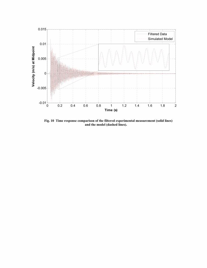
In order to compare the responses in the time domain, a filter was applied to eliminate the rigid body motion. The measured response was filtered using a fourth order Butterworth filter, with frequencies between 50 and 600 Hz kept. Note that other frequency ranges were also used and it was noted that including higher frequencies in the filtering process did not change the time response significantly. The filtered, measured response is compared to the superposition of the responses of the three modal Iwan models in Fig. 10.
Fig. 10 about here.
The velocity ring-down for the model (dashed line) is observed to compare very well with the ring-down of the filtered measurement (solid line). The overall decay envelope of the response is captured very well and the amplitude and phase of the signals agree remarkably well over any time interval. In this type of comparison, it is important to note that the measured data has been filtered and this could distort the signals, but in this case the distortion would hopefully be minimal since only the rigid body motions have been eliminated.
8. Conclusions
In this work, a viscous damper was added in parallel with a modal Iwan model and a procedure was discussed to identify parameters for the model from laboratory data. The 4-parameter Iwan model was found to fit the measurements very well for the first three bending modes, suggesting that modal coupling was weak and that a modal Iwan model may be an effective way of accounting for the nonlinear damping associated with the mechanical joints of the system. The measurements also showed that it was important to also have a viscous damper in parallel with the Iwan element in order to account for the linear damping
associated with the material and the boundary conditions. There are only a few parameters to identify and the parameters , , C and KT are all fairly clearly represented in the modal response. On the other hand, in this study FS and K∞ were somewhat difficult to estimate since we were not able to apply large enough input forces to drive the system well into the macro-slip regime. This is likely to always be a problem when impulsive forces are used since the joint dissipates a lot of energy in the first few cycles, before the filters and Hilbert transform have stabilized.
This modal Iwan approach is very appealing since it allows one to treat a structure as a set of uncoupled linear modes with slightly nonlinear characteristics in the micro-slip regime; a collection of modal Iwan models such as this is extremely inexpensive to integrate, making this approach very attractive whenever the force levels are low enough that the approach is applicable. Indeed, even when performing high fidelity, predictive simulations of a structure (see, e.g. [11-13]) it may be worthwhile to first use the high fidelity model to derive an equivalent modal Iwan model for each mode of interest and then to use those simple models to compute the time response of the structure.
In the validation section, this model was used to predict the response of the structure to a measured impulsive force and the comparison showed that the modal Iwan model did accurately predict the measured response over the frequency range of interest. Future works will further explore the validity of the modal model, by using inputs at other locations and other types of inputs. To date, experimental and analytical results have suggested that this approach can be very successful, except perhaps at very high force levels when serious macro-slip occurs [7].
Acknowledgments The experimental work for this paper was conducted at Sandia National Laboratories.
Sandia is a multi-program laboratory operated under Sandia Corporation, a Lockheed Martin Company, for the United States Department of Energy under Contract DE-AC04-94-AL85000. The authors would especially like to thank Jill Blecke, Randall Mayes, Brandon Zwink and Patrick Hunter for the help that they provided with the laboratory setup and testing.
References [1] D. J. Segalman, "An Initial Overview of Iwan Modelling for Mechanical Joints,"
Sandia National Laboritories, Albuquerque, New Mexico SAND2001-0811, 2001. [2] D. J. Segalman, "A Four-Parameter Iwan Model for Lap-Type Joints," Journal of
Applied Mechanics, vol. 72, pp. 752-760, September 2005. [3] D. J. Segalman and M. J. Starr, "Iwan models and their provenance," presented at the
ASME 2012 International Design Engineering Technical Conferences and Computers and Information in Engineering Conference, Chicago, IL, 2012.
[4] M. S. Allen and R. L. Mayes, "Estimating the degree of nonlinearity in transient responses with zeroed early-time fast Fourier transforms," Mechanical Systems and Signal Processing, vol. 24, pp. 2049-2064, 2010.
[5] D. J. Segalman and W. Holzmann, "Nonlinear Response of a Lap-Type Joint using a Whole-Interface Model," presented at the 23rd International Modal Analysis Conference (IMAC-XXIII), Orlando, Florida, 2005.
[6] D. J. Segalman, "A Modal Approach to Modeling Spatially Distributed Vibration Energy Dissipation," Sandia National Laboratories, Albuquerque, New Mexico and Livermore, California SAND2010-4763, 2010.
[7] B. J. Deaner, M. S. Allen, M. J. Starr, and D. J. Segalman, "Investigation of Modal Iwan Models for Structures with Bolted Joints," presented at the International Modal Analysis Conference XXXI, Garden Grove, California USA, 2013.
[8] M. Eriten, M. Kurt, G. Luo, D. Michael McFarland, L. A. Bergman, and A. F. Vakakis, "Nonlinear system identification of frictional effects in a beam with a bolted joint connection," Mechanical Systems and Signal Processing, vol. 39, pp. 245-264, 2013.
[9] P. Reuss, S. Kruse, S. Peter, F. Morlock, and L. Gaul, "Identification of nonlinear joint characteristic in dynamic substructuring," in 31st IMAC, A Conference on Structural Dynamics, 2013, February 11, 2013 - February 14, 2013, Garden Grove, CA, United states, 2014, pp. 27-36.
[10] P. Reuss, B. Zeumer, J. Herrmann, and L. Gaul, "Consideration of interface damping in dynamic substructuring," in 30th IMAC, A Conference on Structural Dynamics, 2012, January 30, 2012 - February 2, 2012, Jacksonville, FL, United states, 2012, pp. 81-88.
[11] S. Bograd, P. Reuss, A. Schmidt, L. Gaul, and M. Mayer, "Modeling the dynamics of mechanical joints," Mechanical Systems and Signal Processing, vol. 25, pp. 2801-2826, 2011.
[12] C. Hammami and E. Balmes, "Meta-models of repeated dissipative joints for damping design phase," presented at the International Seminar on Modal Analysis (ISMA), Leuven, Belgium, 2014.
[13] E. P. Petrov and D. J. Ewins, "Analytical Formulation of Friction Interface Elements for Analysis of Nonlinear Multi-Harmonic Vibrations of Bladed Disks," Journal of Turbomachinery, vol. 125, pp. 364-371, 2003.
[14] D. J. Segalman, D. L. Gregory, M. J. Starr, B. R. Resor, M. D. Jew, J. P. Lauffer, and N. M. Ames, "Handbook on Dynamics of Jointed Structures," Sandia National Laboratories, Albuquerque, NM2009.
[15] D. L. Gregory, Resor, B. R., Coleman, R. G., "Experimental Investigations of an Inclined Lap-Type Bolted Joint," Sandia National Laboritories, Albuquerque, New Mexico SAND2003-1193, 2003.
[16] M. W. Sracic, M. S. Allen, and H. Sumali, "Identifying the modal properties of nonlinear structures using measured free response time histories from a scanning laser Doppler vibrometer," presented at the International Modal Analysis Conference XXX, Jacksonville, Florida USA, 2012.
[17] Q. Zhang, Allemang, R. J. , Brown, D. L., "Modal Filter: Concept and Application," presented at the 8th International Modal Analysis Conference (IMAC VIII), Kissimmee, Flordia, 1990.
[18] S. D. Stearns, Digital Signal Processing with Examples in Matlab. New York: CRC Press, 2003.
[19] S. Braun and M. Feldman, "Decomposition of non-stationary signals into varying time scales: Some aspects of the EMD and HVD methods," 2011.
[20] H. Sumali and R. A. Kellogg, "Calculating Damping from Ring-Down Using Hilbert Transform and Curve Fitting," presented at the 4th International Operational Modal Analysis Conference (IOMAC), Istanbul, Turkey, 2011.
[21] M. Feldman, "Hilbert transform in vibration analysis," Mechanical Systems and Signal Processing, vol. 25, pp. 735-802, 2011.
[22] G. Kerschen, A. F. Vakakis, Y. S. Lee, D. M. McFarland, and L. A. Bergman, "Toward a fundamental understanding of the Hilbert-Huang transform in nonlinear structural dynamics," JVC/Journal of Vibration and Control, vol. 14, pp. 77-105, 2008.
[23] D. R. Jones, Perttunen, C. D., Stuckman, B. E., "Lipschitzian Optimization Without the Lipschitz Constant," Journal of Optimization Theory and Application, vol. 79, pp. 157-181, 1993.
[24] "Optimization Toolbox For Use with MATLAB," ed. Natick, MA: The MathWorks, Inc., 2003.
[25] S. M. Dickinson, "On the Use of Simply Supported Plate Functions in Raleigh's Method Applied to the Flexural Vibration of Rectangular Plates," Journal of Sound and Vibration, vol. 59, pp. 143-146, 1978.
[26] T. G. Carne, D. T. Griffith, and M. E. Casias, "Support Conditions for Experimental Modal Analysis," Sound and Vibration, vol. 41, pp. 10-16, 2007.
[27] H. Sumali, "An experiment setup for studying the effect of bolt torque on damping," presented at the 4th International Conference on Experimental Vibration Analysis for Civil Engineering Structures (EVACES), Varenna, Italy, 2011.
[28] M. S. Allen and J. H. Ginsberg, "A Global, Single-Input-Multi-Output (SIMO) Implementation of The Algorithm of Mode Isolation and Applications to Analytical and Experimental Data," Mechanical Systems and Signal Processing, vol. 20, pp. 1090-1111, 2006.
[29] M. S. Allen and J. H. Ginsberg, "Global, hybrid, MIMO implementation of the algorithm of mode isolation," in 23rd International Modal Analysis Conference (IMAC XXIII), 2005.
Fig. 1 Schematic of the model for each modal degree of freedom. Each mode has a unique set of Iwan parameters that characterize its nonlinear damping and a viscous damper that captures the linear component of the damping.
M = 1 , , ,S TF K
C
K∞
q
Fig. 2 Photograph of the two beam test structure.
Fig. 3 Photograph of the suspension setup for the two beam test structure.
-0.2-0.1
00.1
0.2-0.5
00.5
1st Elastic Mode 120.9 Hz
-0.2-0.1 0
0.10.2
-1
0
1
2nd Elastic Mode 214.8 Hz
-0.2-0.1
00.1
0.2-1
0
1
3rd Elastic Mode 473.7 Hz
-0.2-0.1
00.1
0.20
0.51
4th Elastic Mode 787.4 Hz
-0.2-0.1
00.1
0.2
0.20.40.60.811.21.4
5th Elastic Mode 813.2 Hz
-0.2-0.1
00.1
0.2
00.5
11.5
6th Elastic Mode 1050 Hz
Fig. 4 Two beam mass normalized mode shapes at 3.39 N-m torque.
10-2
10-1
100
113
114
115
116
117
118
119
120
121
122
Modal Force
Nat
ura
l F
req
uen
cy (
Hz)
Two Beam 1st Mode 3.39 N-m
Lab Data
Modal Iwan ModelModal Iwan & VD Model
Fig. 5 Comparison between measured natural frequency vs. force and two models.
10-2
10-1
100
10-12
10-10
10-8
10-6
Modal Force
Mo
dal
En
erg
y D
issi
pat
ion
/Cyc
le
Two Beam 1st Mode 3.39 N-m
Lab Data
Modal Iwan ModelModal Iwan & VD Model
VD Model
Fig. 6 Energy dissipation comparison of two optimized modal models to experimental data over a range of forces.
10-2
10-1
100
2
2.5
3
3.5
4
Modal Force
Slo
pe
of
En
erg
y D
issi
pat
ion
Cu
rve
Two Beam 1st Mode 3.39 N-m
Fitted Lab Data
Iwan ModelIwan & VD Model
VD Model
Fig. 7 Slope of energy dissipation versus modal force for modal Iwan models and a polynomial fit to the experimental measurements.
0 100 200 300 400 500 600 700 80010
-8
10-7
10-6
10-5
10-4
10-3
Frequency (Hz)
|Vel
oci
ty|
(m/s
)FFT of Velocity at Midpoint
0.051
0.29
0.53
0.76
1
0.051
0.29
0.53
0.76
1
Fig. 8 ZEFFTs for the midpoint of the structure for both the experimental measurement (solid lines) and the model (dashed lines).
117 118 119 120 121 122 123 124
10-6
10-5
10-4
Frequency (Hz)
|Vel
oci
ty|
(m/s
)
FFT of Velocity at Midpoint
Fig. 9 Zoomed in view of the first resonant peak with ZEFFTs for the both the experimental measurement (solid lines) and the model (dashed lines).
0 0.2 0.4 0.6 0.8 1 1.2 1.4 1.6 1.8 2-0.01
-0.005
0
0.005
0.01
0.015V
elo
city
(m
/s)
at M
idp
oin
t
Time (s)
Filtered Data
Simulated Model
Fig. 10 Time response comparison of the filtered experimental measurement (solid lines) and the model (dashed lines).