Applications of Artificial Intelligence and MachineLearning in Othello

Jack Chen

tjhsst Computer Systems Lab 2009–2010

Abstract

This project explores Artificial Intelligence techniques in the board game Othello.Several Othello-playing programs were implemented and compared. The performanceof minimax search algorithms, including alpha-beta, NegaScout and MTD(f), and ofother search improvements such as transposition tables, was analyzed. In addition, theuse of machine learning to enable AI players to improve play automatically throughtraining was investigated.

1 Introduction

Othello (also known as Reversi) is a two-player board game and abstract strategy game, likechess and checkers. I chose to work with Othello because it is sufficiently complex to allowsignificant exploration of advanced AI techniques, but has a simple set of rules compared tomore complex games like chess. It has a moderate branching factor, larger than checkers andsmaller than chess, for example, which makes advanced search techniques important withoutrequiring a great deal of computational power for strong play. Although my AI programsare implemented to play Othello, most of the algorithms, data structures, and techniquesI have investigated are designed for abstract strategy games in general instead of Othellospecifically, and many machine learning algorithms are widely applicable to problems otherthan games.

2 Background

The basic goal of an AI player is to consider the possible moves from the current gamestate, evaluate the position resulting from each move, and choose the one that appears best.One major component of an AI player is the static evaluation function, which heuristicallyestimates the value of a position without exploring moves. This value indicates which playerhas the advantage and how large that advantage is. A second major component is the searchalgorithm, which more accurately evaluates a state by looking ahead at potential moves.

1

3 Static Evaluation

3.1 Features

For positions at the end of a game, the static evaluation is based solely on the number ofpieces each player has, but for earlier positions, other positional features must be considered.The primary goals before the end of the game are mobility, stability, and parity. The majorfeatures used in my static evaluation function reflect these three goals. The overall evaluationis a linear combination of the features, that is, it is a weighted sum of the feature values.Features that are good have positive weights, while features that are bad have negativeweights, and the magnitude of a feature’s weight reflects its importance.

• Mobility

Mobility is a measure of the number of moves available to each player, both at thecurrent position and in the future (potential mobility). Mobility is important becausea player with low mobility is more likely to be forced to make a bad move, such asgiving up a corner. The goal is to maximize one’s own mobility and minimize theopponent’s mobility.

– Moves

The number of moves each player can make is a measure of current mobility.The moves differential, the number of moves available to the player minus thenumber of moves available to the opponent, is one of the features used in mystatic evaluation function. Positions with higher moves differential are better forthat player, so this feature has a positive weight.

– Frontier squares

Frontier squares are empty squares adjacent to a player’s pieces. The numberof frontier squares is a measure of potential mobility, because the more frontiersquares a player has, the more moves the opponent can potentially make. Havingfewer frontier squares than the opponent is good, so the frontier squares differentialis weighted negatively.

• Stability

Pieces that are impossible to flip are called stable. These pieces are useful becausethey contribute directly to the final score.

– Corners

Corners are extremely valuable because corner pieces are immediately stable andcan make adjacent pieces stable. They have the largest positive weights of all thefeatures I use.

2

– X-squares

X-squares are the squares diagonally adjacent to corners. X-squares are highlyundesirable when the adjacent corner is unoccupied because they make the cornervulnerable to being taken by the opponent, so they have very negative weight.

– C-squares

C-squares are the squares adjacent to corners and on an edge. C-squares adjacentto an unoccupied corner are somewhat undesirable, like X-squares, but they aremuch less dangerous. In addition, C-squares can contribute to edge stability,which makes them desirable in some cases. Generally, C-squares are weightedfairly negatively, but to a much smaller extent than X-squares.

• Parity

Global parity is the strategic concept that the last player to move in the game has aslight advantage because all of the pieces gained become stable. White therefore hasan advantage over black, as long as the parity is not reversed by passes. In addition,in the endgame, empty squares tend to separate into disjoint regions. Local parity isbased on the idea that the last player to move in each region has an advantage becausethe pieces that player gains are often stable. I use global parity as a feature, but donot consider local parity.

3.2 Game Stages

The importance of the features used in the static evaluation function depends on the stageof the game. For example, one common strategy is to minimize the number of pieces onehas early in the game, as this tends to improve mobility, even though this is contrary to theultimate goal of the game. It is useful, then, to have different feature weights for differentgame stages. In Othello, the total number of pieces on the board is a good measure of thegame stage.

4 Search Algorithms and Data Structures

Static evaluation is often inaccurate. For example, it is difficult to detect traps statically.When evaluating a position, it is therefore important to consider possible moves, the possiblemoves in response to each of those moves, and so on. This forms a game tree of the possiblesequences of moves from the initial game state.

4.1 Minimax

The minimax search algorithm is the basic algorithm to do this exploration of the gametree. Minimax recursively evaluates a position by taking the best of the values for each childposition. The best value is the maximum for one player and the minimum for the otherplayer, because positions that are good for one player are bad for the other.

3

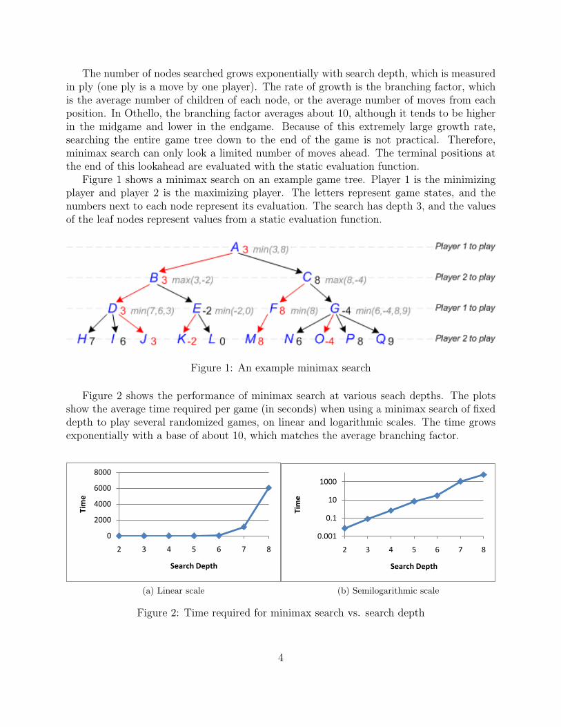
The number of nodes searched grows exponentially with search depth, which is measuredin ply (one ply is a move by one player). The rate of growth is the branching factor, whichis the average number of children of each node, or the average number of moves from eachposition. In Othello, the branching factor averages about 10, although it tends to be higherin the midgame and lower in the endgame. Because of this extremely large growth rate,searching the entire game tree down to the end of the game is not practical. Therefore,minimax search can only look a limited number of moves ahead. The terminal positions atthe end of this lookahead are evaluated with the static evaluation function.

Figure 1 shows a minimax search on an example game tree. Player 1 is the minimizingplayer and player 2 is the maximizing player. The letters represent game states, and thenumbers next to each node represent its evaluation. The search has depth 3, and the valuesof the leaf nodes represent values from a static evaluation function.

Figure 1: An example minimax search

Figure 2 shows the performance of minimax search at various seach depths. The plotsshow the average time required per game (in seconds) when using a minimax search of fixeddepth to play several randomized games, on linear and logarithmic scales. The time growsexponentially with a base of about 10, which matches the average branching factor.

0

2000

4000

6000

8000

2 3 4 5 6 7 8

Tim

e

Search Depth

(a) Linear scale

0.001

0.1

10

1000

2 3 4 5 6 7 8

Tim

e

Search Depth

(b) Semilogarithmic scale

Figure 2: Time required for minimax search vs. search depth

4

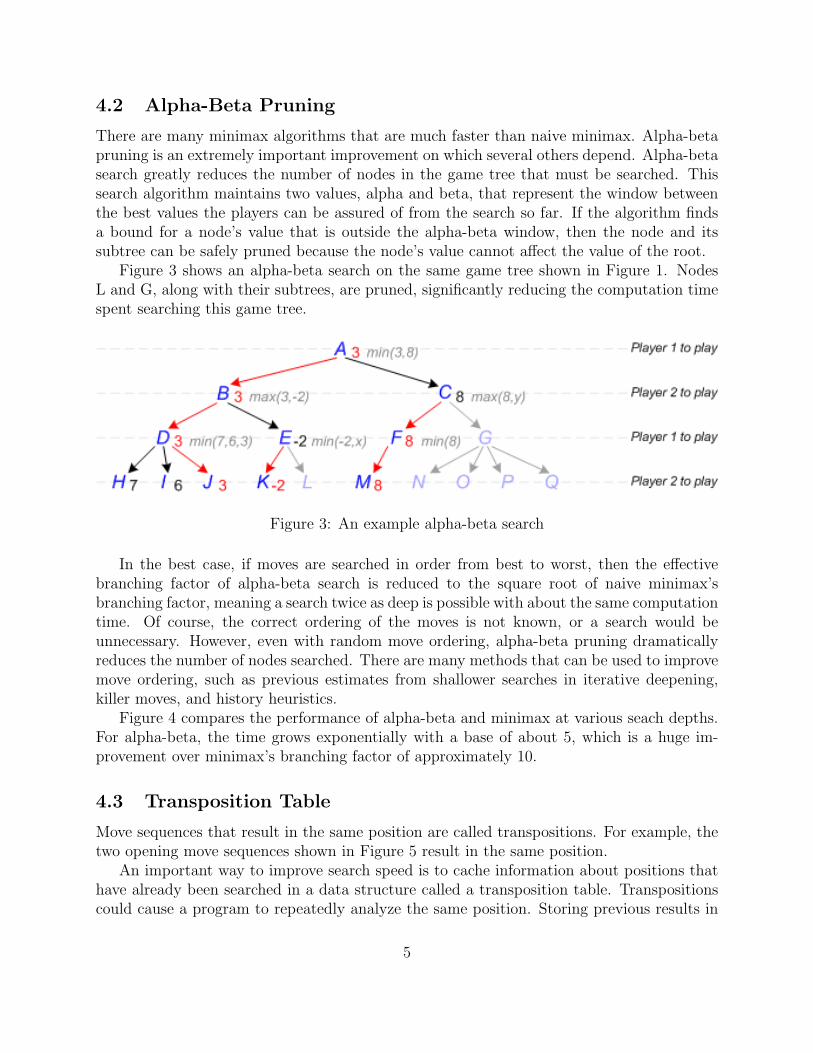
4.2 Alpha-Beta Pruning

There are many minimax algorithms that are much faster than naive minimax. Alpha-betapruning is an extremely important improvement on which several others depend. Alpha-betasearch greatly reduces the number of nodes in the game tree that must be searched. Thissearch algorithm maintains two values, alpha and beta, that represent the window betweenthe best values the players can be assured of from the search so far. If the algorithm findsa bound for a node’s value that is outside the alpha-beta window, then the node and itssubtree can be safely pruned because the node’s value cannot affect the value of the root.

Figure 3 shows an alpha-beta search on the same game tree shown in Figure 1. NodesL and G, along with their subtrees, are pruned, significantly reducing the computation timespent searching this game tree.

Figure 3: An example alpha-beta search

In the best case, if moves are searched in order from best to worst, then the effectivebranching factor of alpha-beta search is reduced to the square root of naive minimax’sbranching factor, meaning a search twice as deep is possible with about the same computationtime. Of course, the correct ordering of the moves is not known, or a search would beunnecessary. However, even with random move ordering, alpha-beta pruning dramaticallyreduces the number of nodes searched. There are many methods that can be used to improvemove ordering, such as previous estimates from shallower searches in iterative deepening,killer moves, and history heuristics.

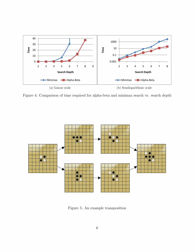
Figure 4 compares the performance of alpha-beta and minimax at various seach depths.For alpha-beta, the time grows exponentially with a base of about 5, which is a huge im-provement over minimax’s branching factor of approximately 10.

4.3 Transposition Table

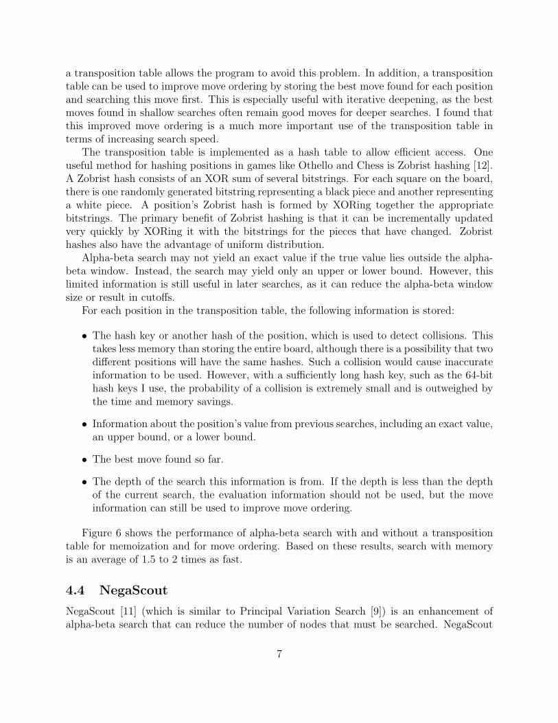
Move sequences that result in the same position are called transpositions. For example, thetwo opening move sequences shown in Figure 5 result in the same position.

An important way to improve search speed is to cache information about positions thathave already been searched in a data structure called a transposition table. Transpositionscould cause a program to repeatedly analyze the same position. Storing previous results in

5

0

10

20

30

40

2 3 4 5 6 7 8 9

Tim

e

Search Depth

Minimax Alpha-Beta

(a) Linear scale

0.001

0.1

10

1000

2 3 4 5 6 7 8

Tim

e

Search Depth

Minimax Alpha-Beta

(b) Semilogarithmic scale

Figure 4: Comparison of time required for alpha-beta and minimax search vs. search depth

Figure 5: An example transposition

6

a transposition table allows the program to avoid this problem. In addition, a transpositiontable can be used to improve move ordering by storing the best move found for each positionand searching this move first. This is especially useful with iterative deepening, as the bestmoves found in shallow searches often remain good moves for deeper searches. I found thatthis improved move ordering is a much more important use of the transposition table interms of increasing search speed.

The transposition table is implemented as a hash table to allow efficient access. Oneuseful method for hashing positions in games like Othello and Chess is Zobrist hashing [12].A Zobrist hash consists of an XOR sum of several bitstrings. For each square on the board,there is one randomly generated bitstring representing a black piece and another representinga white piece. A position’s Zobrist hash is formed by XORing together the appropriatebitstrings. The primary benefit of Zobrist hashing is that it can be incrementally updatedvery quickly by XORing it with the bitstrings for the pieces that have changed. Zobristhashes also have the advantage of uniform distribution.

Alpha-beta search may not yield an exact value if the true value lies outside the alpha-beta window. Instead, the search may yield only an upper or lower bound. However, thislimited information is still useful in later searches, as it can reduce the alpha-beta windowsize or result in cutoffs.

For each position in the transposition table, the following information is stored:

• The hash key or another hash of the position, which is used to detect collisions. Thistakes less memory than storing the entire board, although there is a possibility that twodifferent positions will have the same hashes. Such a collision would cause inaccurateinformation to be used. However, with a sufficiently long hash key, such as the 64-bithash keys I use, the probability of a collision is extremely small and is outweighed bythe time and memory savings.

• Information about the position’s value from previous searches, including an exact value,an upper bound, or a lower bound.

• The best move found so far.

• The depth of the search this information is from. If the depth is less than the depthof the current search, the evaluation information should not be used, but the moveinformation can still be used to improve move ordering.

Figure 6 shows the performance of alpha-beta search with and without a transpositiontable for memoization and for move ordering. Based on these results, search with memoryis an average of 1.5 to 2 times as fast.

4.4 NegaScout

NegaScout [11] (which is similar to Principal Variation Search [9]) is an enhancement ofalpha-beta search that can reduce the number of nodes that must be searched. NegaScout

7

0

50

100

150

4 5 6 7 8 9 10

Tim

e

Search Depth

Without Memory With Memory

(a)

40%

50%

60%

70%

80%

90%

4 5 6 7 8 9 10

Re

lati

ve T

ime

Search Depth

(b) Time for alpha-beta with memory relative toalpha-beta without memory

Figure 6: Comparison of time required for alpha-beta search with and without a transpositiontable vs. search depth

searches the first move for a node with a normal alpha-beta window. It then assumes thatthe next moves are worse, which is often true with good move ordering. For the remainingmoves, it uses a null-window search, in which the alpha-beta window has zero width, totest whether this is true. The value must lie outside the null-window, so the null-windowsearch must fail. However, this yields a lower or upper bound on the value if the null-windowsearch fails high or low, respectively. If it fails low, then the test successfully shows that themove is worse than the current alpha and therefore does not need to be further considered.Otherwise, the test shows that the move is better than the current alpha, so it must bere-searched with a full window.

Null-window searches are faster because they produce many more cutoffs. However, eventhough NegaScout never explores nodes that alpha-beta prunes, NegaScout may be slowerbecause it may need to re-search nodes several times when null-window searches fail high.If move ordering is good, NegaScout searches faster than alpha-beta pruning, but if moveordering is poor, NegaScout can be slower. See Section 4.6 for analysis of the performanceof NegaScout.

A transposition table is even more beneficial to NegaScout than to alpha-beta becausestored information can be used during re-searches, for example, to prevent re-evaluation ofleaf nodes.

4.5 MTD(f)

MTD(f) [10] is another search algorithm that is more efficient than alpha-beta and outper-forms NegaScout. It is efficient because it uses only null-window searches, which result inmany more cutoffs than wide window alpha-beta searches. Each null-window search yieldsa bound on the minimax value, so MTD(f) uses repeated null-window searches to converge

8

on the exact minimax value. Because many nodes need to be re-evaluated several times, atransposition table is crucial for MTD(f) to prevent excessive re-searches.

MTD(f) starts its search at a given value, f. The speed of MTD(f) depends heavily onhow close this first guess is to the actual value, as the closer it is the fewer null-windowsearches are necessary. It is therefore useful to use iterative deepening on MTD(f), using thevalue of the previous iteration as the first guess for the next iteration.

While MTD(f) is theoretically more efficient than alpha-beta and NegaScout, it has somepractical issues, such as heavy reliance on the transposition table and search instability. Theperformance of MTD(f) is discussed in Section 4.6.

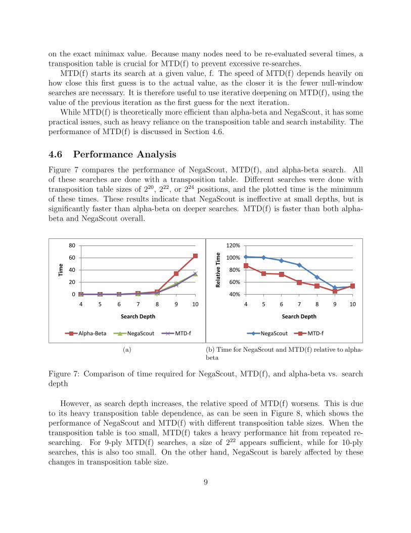
4.6 Performance Analysis

Figure 7 compares the performance of NegaScout, MTD(f), and alpha-beta search. Allof these searches are done with a transposition table. Different searches were done withtransposition table sizes of 220, 222, or 224 positions, and the plotted time is the minimumof these times. These results indicate that NegaScout is ineffective at small depths, but issignificantly faster than alpha-beta on deeper searches. MTD(f) is faster than both alpha-beta and NegaScout overall.

0

20

40

60

80

4 5 6 7 8 9 10

Tim

e

Search Depth

Alpha-Beta NegaScout MTD-f

(a)

40%

60%

80%

100%

120%

4 5 6 7 8 9 10

Re

lati

ve T

ime

Search Depth

NegaScout MTD-f

(b) Time for NegaScout and MTD(f) relative to alpha-beta

Figure 7: Comparison of time required for NegaScout, MTD(f), and alpha-beta vs. searchdepth

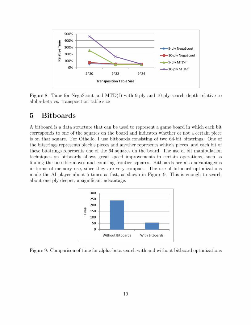
However, as search depth increases, the relative speed of MTD(f) worsens. This is dueto its heavy transposition table dependence, as can be seen in Figure 8, which shows theperformance of NegaScout and MTD(f) with different transposition table sizes. When thetransposition table is too small, MTD(f) takes a heavy performance hit from repeated re-searching. For 9-ply MTD(f) searches, a size of 222 appears sufficient, while for 10-plysearches, this is also too small. On the other hand, NegaScout is barely affected by thesechanges in transposition table size.

9

0%

100%

200%

300%

400%

500%

2^20 2^22 2^24

Re

lati

ve T

ime

Transposition Table Size

9-ply NegaScout

10-ply NegaScout

9-ply MTD-f

10-ply MTD-f

Figure 8: Time for NegaScout and MTD(f) with 9-ply and 10-ply search depth relative toalpha-beta vs. transposition table size

5 Bitboards

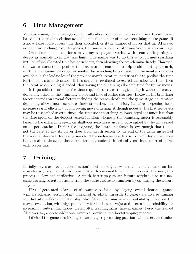
A bitboard is a data structure that can be used to represent a game board in which each bitcorresponds to one of the squares on the board and indicates whether or not a certain pieceis on that square. For Othello, I use bitboards consisting of two 64-bit bitstrings. One ofthe bitstrings represents black’s pieces and another represents white’s pieces, and each bit ofthese bitstrings represents one of the 64 squares on the board. The use of bit manipulationtechniques on bitboards allows great speed improvements in certain operations, such asfinding the possible moves and counting frontier squares. Bitboards are also advantageousin terms of memory use, since they are very compact. The use of bitboard optimizationsmade the AI player about 5 times as fast, as shown in Figure 9. This is enough to searchabout one ply deeper, a significant advantage.

0

50

100

150

200

250

300

Without Bitboards With Bitboards

Time

Figure 9: Comparison of time for alpha-beta search with and without bitboard optimizations

10

6 Time Management

My time management strategy dynamically allocates a certain amount of time to each movebased on the amount of time available and the number of moves remaining in the game. Ifa move takes more or less time than allocated, or if the number of moves that my AI playerneeds to make changes due to passes, the time allocated to later moves changes accordingly.

Once time is allocated for a move, my AI player searches with iterative deepening asdeeply as possible given the time limit. One simple way to do this is to continue searchinguntil all of the allocated time has been spent, then aborting the search immediately. However,this wastes some time spent on the final search iteration. To help avoid aborting a search,my time management strategy estimates the branching factor, based on the number of movesavailable in the leaf nodes of the previous search iteration, and uses this to predict the timefor the next search iteration. If this search is predicted to exceed the allocated time, thenthe iterative deepening is ended, thus saving the remaining allocated time for future moves.

It is possible to estimate the time required to search to a given depth without iterativedeepening based on the branching factor and time of earlier searches. However, the branchingfactor depends on several factors including the search depth and the game stage, so iterativedeepening allows more accurate time estimation. In addition, iterative deepening helpsincrease search efficiency by improving move ordering. Although nodes at the first few levelsmay be re-searched several times, the time spent searching at lower depths is much less thanthe time spent on the deepest search iteration whenever the branching factor is reasonablylarge, so the extra time spent on shallower searches is usually outweighed by the time savedon deeper searches. During the endgame, the branching factor is low enough that this isnot the case, so my AI player does a full-depth search to the end of the game instead ofthe normal iterative deepening search. This endgame search also is much faster per nodebecause all static evaluation at the terminal nodes is based soley on the number of pieceseach player has.

7 Training

Initially, my static evaluation function’s feature weights were set manually based on hu-man strategy, and hand-tuned somewhat with a manual hill-climbing process. However, thisprocess is slow and ineffective. A much better way to set feature weights is to use ma-chine learning to automatically train the static evaluation function by optimizing the featureweights.

First, I generated a large set of example positions by playing several thousand gameswith a stochastic version of my untrained AI player. In order to generate a diverse trainingset that also reflects realistic play, this AI chooses moves with probability based on themove’s evaluation, with high probability for the best move(s) and decreasing probability forincreasingly suboptimal moves. Later, after training using these examples, I used the trainedAI player to generate additional example positions in a bootstrapping process.

I divided the game into 59 stages, each stage representing positions with a certain number

11

of total pieces from 5 to 63, and trained a separate set of weights for each stage. The trainingprocess starts with the last stage and proceeds through the game stages in reverse order.For each stage, the set of example positions matching the stage are evaluated with a fairlydeep search. For the last few stages of the game, these evaluations are exact because thesearch can reach the end of the game. As earlier stages are trained, the leaf nodes of thesearches are statically evaluated with the weights for a later game stage, which have alreadybeen trained, making the evaluations quite accurate. These evaluations are the target valuesfor the static evaluation function at the current game stage. To optimize the current stage’sweights, I used a batch gradient descent method.

7.1 Gradient Descent

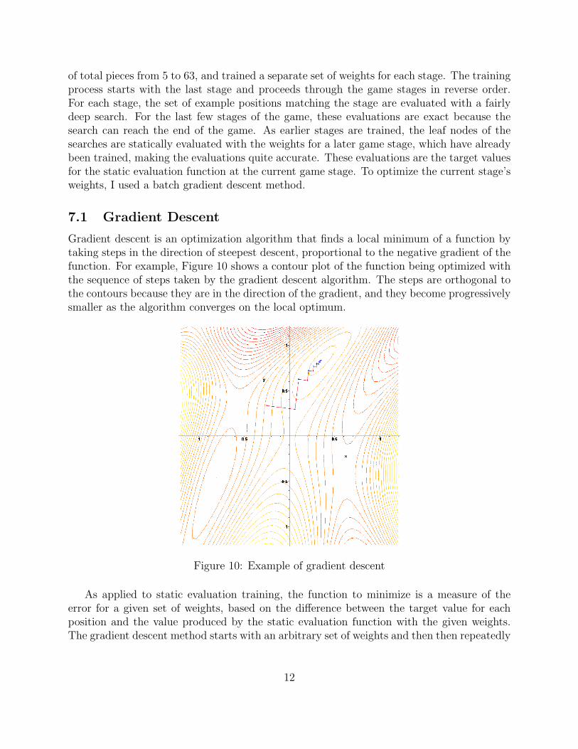
Gradient descent is an optimization algorithm that finds a local minimum of a function bytaking steps in the direction of steepest descent, proportional to the negative gradient of thefunction. For example, Figure 10 shows a contour plot of the function being optimized withthe sequence of steps taken by the gradient descent algorithm. The steps are orthogonal tothe contours because they are in the direction of the gradient, and they become progressivelysmaller as the algorithm converges on the local optimum.

Figure 10: Example of gradient descent

As applied to static evaluation training, the function to minimize is a measure of theerror for a given set of weights, based on the difference between the target value for eachposition and the value produced by the static evaluation function with the given weights.The gradient descent method starts with an arbitrary set of weights and then then repeatedly

12

takes steps in the direction that reduces error most until it reaches convergence at a localminimum.

A basic form of gradient descent takes steps of size directly proportional to the magnitudeof the gradient, with a fixed constant of proportionality called the learning rate. However,a learning rate that is too small may result in extremely slow convergence, while a learningrate that is too large may converge to a poor solution or fail to converge at all. The use ofa dynamic learning rate helps to avoid these problems. In each step, a line search is used todetermine a location along the direction of steepest descent that loosely minimizes the error.

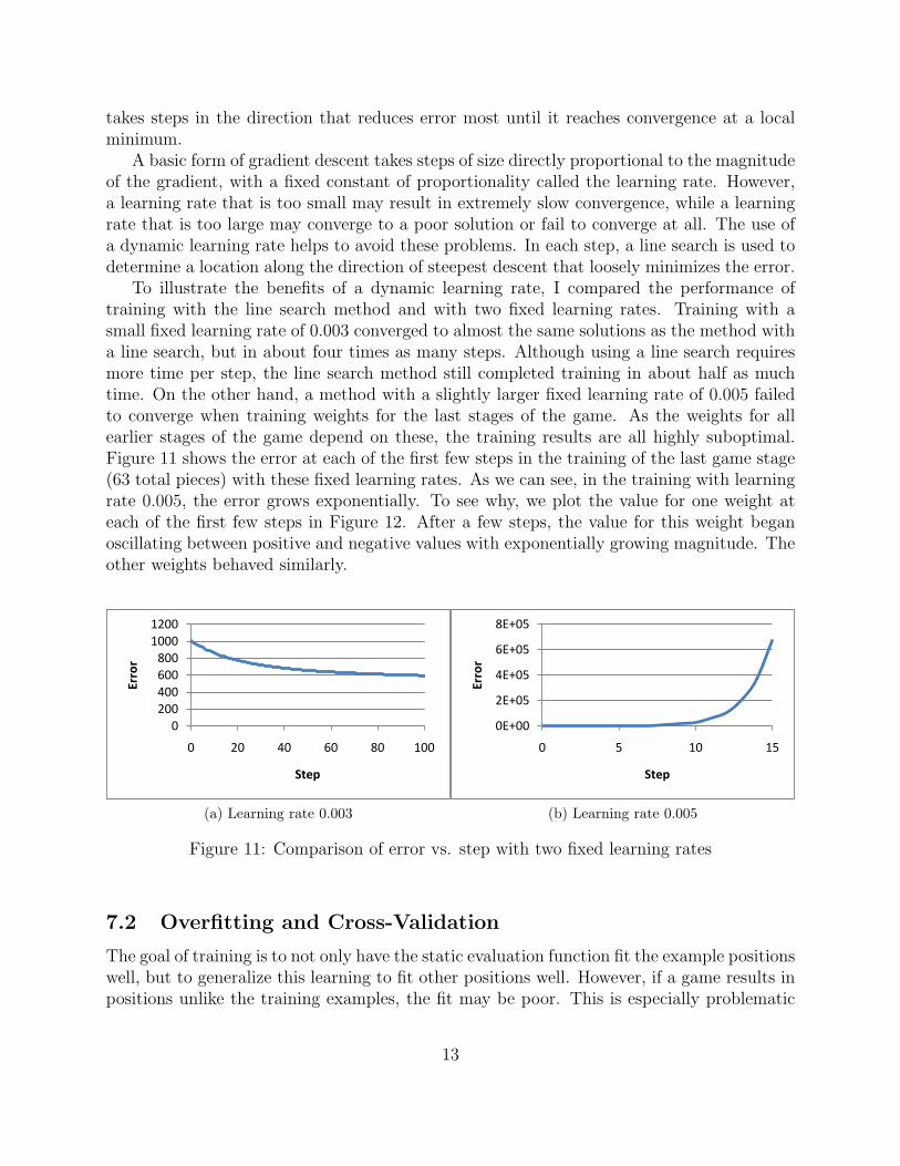
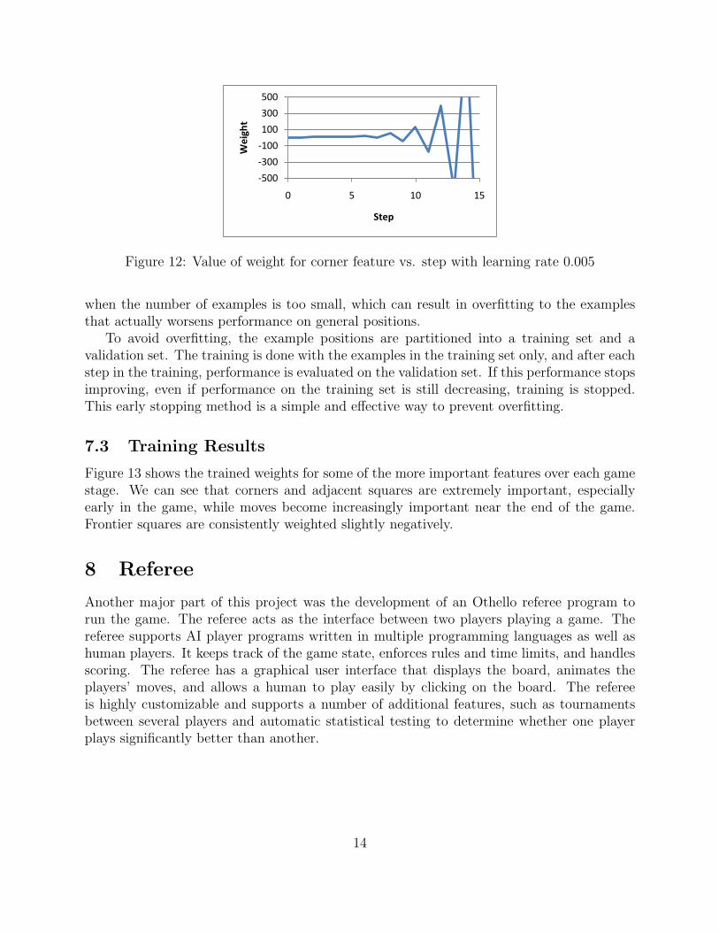
To illustrate the benefits of a dynamic learning rate, I compared the performance oftraining with the line search method and with two fixed learning rates. Training with asmall fixed learning rate of 0.003 converged to almost the same solutions as the method witha line search, but in about four times as many steps. Although using a line search requiresmore time per step, the line search method still completed training in about half as muchtime. On the other hand, a method with a slightly larger fixed learning rate of 0.005 failedto converge when training weights for the last stages of the game. As the weights for allearlier stages of the game depend on these, the training results are all highly suboptimal.Figure 11 shows the error at each of the first few steps in the training of the last game stage(63 total pieces) with these fixed learning rates. As we can see, in the training with learningrate 0.005, the error grows exponentially. To see why, we plot the value for one weight ateach of the first few steps in Figure 12. After a few steps, the value for this weight beganoscillating between positive and negative values with exponentially growing magnitude. Theother weights behaved similarly.

0200400

600800

1000

1200

0 20 40 60 80 100

Error

Step

(a) Learning rate 0.003

0E+00

2E+05

4E+05

6E+05

8E+05

0 5 10 15

Error

Step

(b) Learning rate 0.005

Figure 11: Comparison of error vs. step with two fixed learning rates

7.2 Overfitting and Cross-Validation

The goal of training is to not only have the static evaluation function fit the example positionswell, but to generalize this learning to fit other positions well. However, if a game results inpositions unlike the training examples, the fit may be poor. This is especially problematic

13

-500

-300

-100

100

300

500

0 5 10 15

Weight

Step

Figure 12: Value of weight for corner feature vs. step with learning rate 0.005

when the number of examples is too small, which can result in overfitting to the examplesthat actually worsens performance on general positions.

To avoid overfitting, the example positions are partitioned into a training set and avalidation set. The training is done with the examples in the training set only, and after eachstep in the training, performance is evaluated on the validation set. If this performance stopsimproving, even if performance on the training set is still decreasing, training is stopped.This early stopping method is a simple and effective way to prevent overfitting.

7.3 Training Results

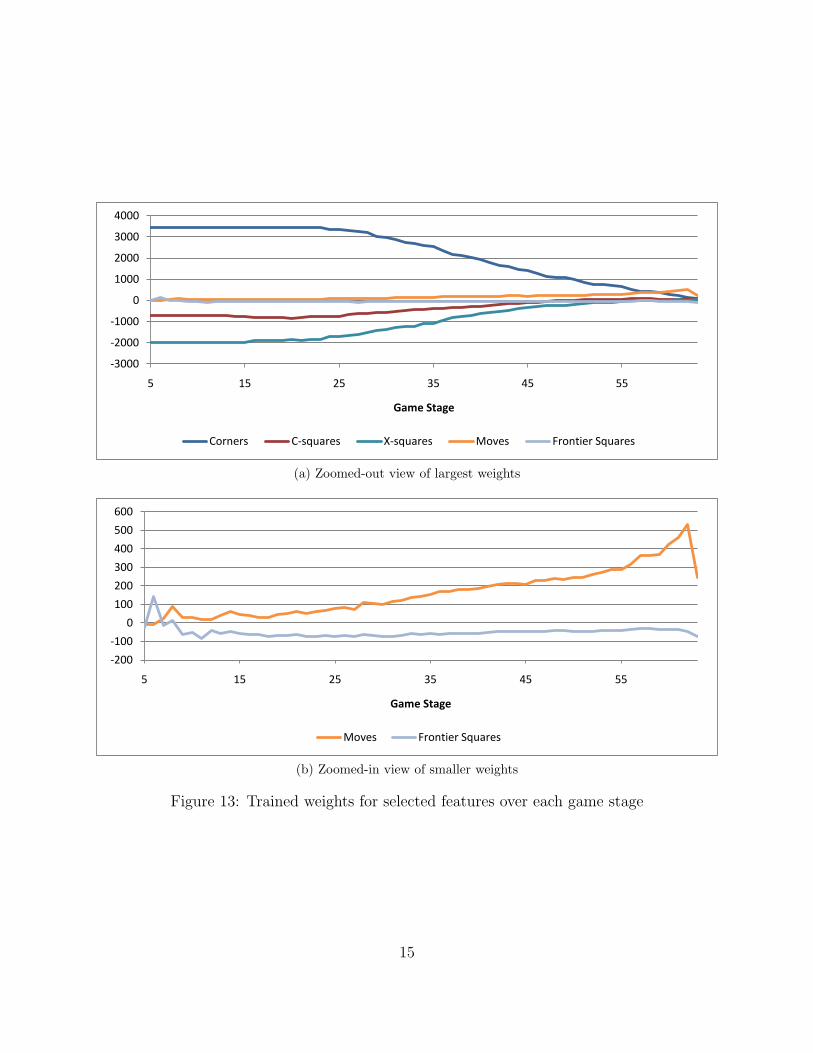
Figure 13 shows the trained weights for some of the more important features over each gamestage. We can see that corners and adjacent squares are extremely important, especiallyearly in the game, while moves become increasingly important near the end of the game.Frontier squares are consistently weighted slightly negatively.

8 Referee

Another major part of this project was the development of an Othello referee program torun the game. The referee acts as the interface between two players playing a game. Thereferee supports AI player programs written in multiple programming languages as well ashuman players. It keeps track of the game state, enforces rules and time limits, and handlesscoring. The referee has a graphical user interface that displays the board, animates theplayers’ moves, and allows a human to play easily by clicking on the board. The refereeis highly customizable and supports a number of additional features, such as tournamentsbetween several players and automatic statistical testing to determine whether one playerplays significantly better than another.

14

1000

-3000

-2000

-1000

0

1000

2000

3000

4000

5 15 25 35 45 55

Game Stage

Corners C-squares X-squares Moves Frontier Squares

(a) Zoomed-out view of largest weights

-3000

-200

-100

0

100

200

300

400

500

600

5 15 25 35 45 55

Game Stage

Moves Frontier Squares

(b) Zoomed-in view of smaller weights

Figure 13: Trained weights for selected features over each game stage

15

9 Conclusions

I implemented and compared several Othello programs using various static evaluation func-tions, search algorithms, and data structures. Search improvements such as transpositiontables and bitboards greatly improve performance, and efficient search algorithms such asNegaScout and MTD(f) are much faster than the basic alpha-beta search algorithm. I foundthat MTD(f) outperformed the other search algorithms I tested. The use of machine learningto optimize the static evaluation function was successful in improving the static evaluation’saccuracy, resulting in better play.

My best AI players were fairly strong, able to easily defeat me and other amateur humanplayers even with extremely small time limits. However, they were not nearly as strong asOthello programs such as Michael Buro’s Logistello [6]. There are many other AI techniquesthat could be explored in future research.

10 Future Research

Selective search algorithms, such as ProbCut [2] and Multi-ProbCut [4] can further enhancegame-tree search by pruning parts of the game tree that probably will not affect the overallminimax value. This allows the player to search much deeper in the relevant parts of thegame tree.

Opening books [5] allow much better and faster play in the early game by storing previ-ously computed information about early game board states.

Another potential area of investigation is parallelization. Splitting up searches betweenseveral processors can greatly increase the search speed.

Traditionally, the static evaluation function is based on human knowledge about thegame. In Othello, static evaluation is usually based on features related to human goals, suchas mobility, stability, and parity. However, using pattern-based features as discussed in [3]can improve static evaluation.

There are several machine learning techniques that can be applied to the training of thestatic evaluation function. Among the algorithms I investigated but did not implement aregenetic algorithms, particle swarm optimization, and artificial neural networks.

There are many other machine learning methods that can be used to improve the qualityand speed of an AI player based on experience. For example, [8] describes the use of an ex-perience base to augment a non-learning Othello program, and [1] describes a chess programthat learns as it plays games using the TDLeaf(λ) algorithm. Another interesting idea is tolearn a model of an opponent’s strategy and incorporate that into the minimax search [7].

16

References

[1] J. Baxter, A. Tridgell, and L. Weaver. Experiments in parameter learning using temporaldifferences. International Computer Chess Association Journal, 21(2):84–99, 1998.

[2] M. Buro. ProbCut: An effective selective extension of the alpha-beta algorithm. Inter-national Computer Chess Association Journal, 18(2):71–76, 1995.

[3] M. Buro. An evaluation function for othello based on statistics. Technical Report 31,NEC Research Institute, 1997.

[4] M. Buro. Experiments with Multi-ProbCut and a new high-quality evaluation functionfor Othello. In H. J. van den Herik and H. Iida, editors, Games in AI Research, pages77–96. Universiteit Maastricht, 2000.

[5] M. Buro. Toward opening book learning. In J. Furnkranz and M. Kubat, editors,Machines that Learn to Play Games, chapter 4, pages 81–89. Nova Science Publishers,Huntington, NY, 2001.

[6] M. Buro. The evolution of strong Othello programs. In Proceedings of the InternationalWorkshop on Entertainment computing (IWEC-02), Makuhari, Japan, 2002.

[7] D. Carmel and S. Markovitch. Learning models of opponent’s strategy in game playing.Technical Report CIS #9305, Centre for Intelligent Systems, Technion - Israel Inst.Technology, Haifa 32000 Israel, Jan. 1993.

[8] K. A. DeJong and A. C. Shultz. Using experience-based learning in game-playing. InProceedings of the 5th International Conference on Machine Learning, pages 284–290,1988.

[9] T. A. Marsland and M. S. Campbell. Parallel search of strongly ordered game trees.ACM Computing Survey, 14(4):533–551, Dec. 1982.

[10] A. Plaat, J. Schaeffer, W. Pijls, and A. de Bruin. A new paradigm for minimax search.Research Note EUR-CS-95-03, Erasmus University Rotterdam, Rotterdam, Nether-lands, 1995.

[11] A. Reinefeld. An improvement of the scout tree search algorithm. ICCA Journal,6(4):4–14, 1983.

[12] A. L. Zobrist. A new hashing method with application for game playing. TechnicalReport 88, Univ. of Wisconsin, 1970.

17