Foundations of Artificial Intelligence 12. Acting under Uncertainty Maximizing Expected Utility Joschka Boedecker and Wolfram Burgard and Frank Hutter and Bernhard Nebel Albert-Ludwigs-Universit¨ at Freiburg July 6, 2018
Transcript
Foundations of Artificial Intelligence12. Acting under Uncertainty
Maximizing Expected Utility
Joschka Boedecker and Wolfram Burgard andFrank Hutter and Bernhard Nebel
Albert-Ludwigs-Universitat Freiburg
July 6, 2018
Contents
1 Introduction to Utility Theory
2 Choosing Individual Actions
3 Sequential Decision Problems
4 Markov Decision Processes
5 Value Iteration
(University of Freiburg) Foundations of AI July 6, 2018 2 / 37
Lecture Overview
1 Introduction to Utility Theory
2 Choosing Individual Actions
3 Sequential Decision Problems
4 Markov Decision Processes
5 Value Iteration
(University of Freiburg) Foundations of AI July 6, 2018 3 / 37
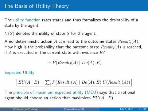
The Basis of Utility Theory
The utility function rates states and thus formalizes the desirability of astate by the agent.
U(S) denotes the utility of state S for the agent.
A nondeterministic action A can lead to the outcome states Result i(A).How high is the probability that the outcome state Result i(A) is reached,if A is executed in the current state with evidence E?
→ P (Result i(A) | Do(A), E)
Expected Utility:
EU(A | E) =∑
i P (Result i(A) | Do(A), E) U(Result i(A))
The principle of maximum expected utility (MEU) says that a rationalagent should choose an action that maximizes EU(A | E).
(University of Freiburg) Foundations of AI July 6, 2018 4 / 37
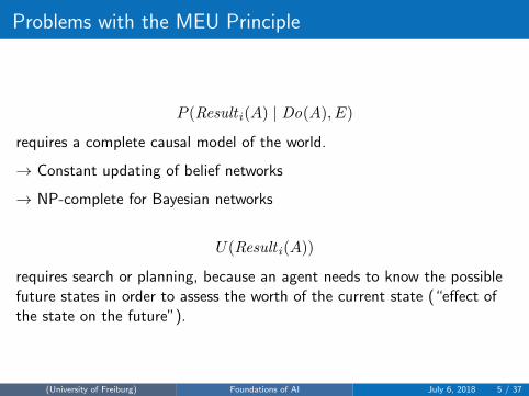
Problems with the MEU Principle
P (Result i(A) | Do(A), E)
requires a complete causal model of the world.
→ Constant updating of belief networks
→ NP-complete for Bayesian networks
U(Result i(A))
requires search or planning, because an agent needs to know the possiblefuture states in order to assess the worth of the current state (“effect ofthe state on the future”).
(University of Freiburg) Foundations of AI July 6, 2018 5 / 37
Lecture Overview
1 Introduction to Utility Theory
2 Choosing Individual Actions
3 Sequential Decision Problems
4 Markov Decision Processes
5 Value Iteration
(University of Freiburg) Foundations of AI July 6, 2018 6 / 37
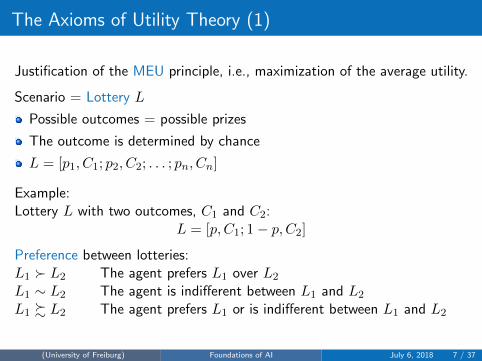
The Axioms of Utility Theory (1)
Justification of the MEU principle, i.e., maximization of the average utility.
Scenario = Lottery L
Possible outcomes = possible prizes
The outcome is determined by chance
L = [p1, C1; p2, C2; . . . ; pn, Cn]
Example:Lottery L with two outcomes, C1 and C2:
L = [p, C1; 1− p, C2]
Preference between lotteries:L1 � L2 The agent prefers L1 over L2
L1 ∼ L2 The agent is indifferent between L1 and L2
L1 % L2 The agent prefers L1 or is indifferent between L1 and L2
(University of Freiburg) Foundations of AI July 6, 2018 7 / 37
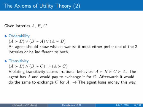
The Axioms of Utility Theory (2)
Given lotteries A, B, C
Orderability(A � B) ∨ (B � A) ∨ (A ∼ B)An agent should know what it wants: it must either prefer one of the 2lotteries or be indifferent to both.
Transitivity(A � B) ∧ (B � C)⇒ (A � C)Violating transitivity causes irrational behavior: A � B � C � A. Theagent has A and would pay to exchange it for C. Afterwards it woulddo the same to exchange C for A. → The agent loses money this way.
(University of Freiburg) Foundations of AI July 6, 2018 8 / 37
The Axioms of Utility Theory (3)
ContinuityA � B � C ⇒ ∃p[p,A; 1− p, C] ∼ BIf some lottery B is between A and C in preference, then there is someprobability p for which the agent is indifferent between getting B forsure and the lottery that yields A with probability p and C withprobability 1− p.
SubstitutabilityA ∼ B ⇒ [p,A; 1− p, C] ∼ [p,B; 1− p, C]If an agent is indifferent between two lotteries A and B, then the agentis indifferent beteween two more complex lotteries that are the sameexcept that B is substituted for A in one of them.
(University of Freiburg) Foundations of AI July 6, 2018 9 / 37
The Axioms of Utility Theory (4)
MonotonicityA � B ⇒ (p > q ⇔ [p,A; 1− p,B] � [q, A; 1− q,B])If an agent prefers the outcome A, then it must also prefer the lotterythat has a higher probability for A.
Decomposability[p,A; 1− p, [q,B; 1− q, C]] ∼ [p,A; (1− p)q,B; (1− p)(1− q), C]Compound lotteries can be reduced to simpler ones using the laws ofprobability. This has been called the “no fun in gambling”-rule: twoconsecutive gambles can be reduced to a single equivalent lottery.
(University of Freiburg) Foundations of AI July 6, 2018 10 / 37
Utility Functions and Axioms
The axioms only make statements about preferences.
The existence of a utility function follows from the axioms!
Utility Principle If an agent’s preferences obey the axioms, then thereexists a function U : S 7→ R withU(A) > U(B)⇔ A � BU(A) = U(B)⇔ A ∼ BExpected Utility of a Lottery:U([p1, S1; . . . ; pn, Sn]) =
∑i pi U(Si)
→ Since the outcome of a nondeterministic action is a lottery, an agentcan act rationally only by following the Maximum Expected Utility(MEU) principle.
How do we design utility functions that cause the agent to act as desired?
(University of Freiburg) Foundations of AI July 6, 2018 11 / 37
Assessing Utilities
The scale of a utility function can be chosen arbitrarily. We therefore candefine a “normalized” utility of a lottery S:
“Best possible prize” U(S) = umax = 1
“Worst catastrophe” U(S) = umin = 0
Given a utility scale between umin and umax we can asses the utility of anyparticular outcome S by asking the agent to choose between S and astandard lottery [p, umax ; 1− p, umin ]. We adjust p until they are equallypreferred.Then, p is the utility of S. This is done for each outcome S to determineU(S).
(University of Freiburg) Foundations of AI July 6, 2018 12 / 37
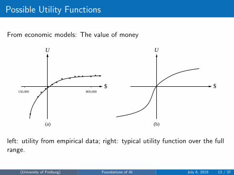
Possible Utility Functions
From economic models: The value of money
U
$ $�150,000 800,000
(a) (b)
o
o
o
oo
oo
o oo o o o o o
U
left: utility from empirical data; right: typical utility function over the fullrange.
(University of Freiburg) Foundations of AI July 6, 2018 13 / 37
Lecture Overview
1 Introduction to Utility Theory
2 Choosing Individual Actions
3 Sequential Decision Problems
4 Markov Decision Processes
5 Value Iteration
(University of Freiburg) Foundations of AI July 6, 2018 14 / 37
Sequential Decision Problems (1)
1 2 3
1
2
3
− 1
+ 1
4
START
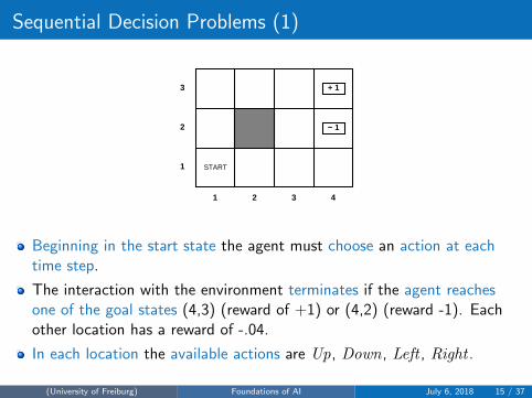
Beginning in the start state the agent must choose an action at eachtime step.
The interaction with the environment terminates if the agent reachesone of the goal states (4,3) (reward of +1) or (4,2) (reward -1). Eachother location has a reward of -.04.
In each location the available actions are Up, Down, Left , Right .
(University of Freiburg) Foundations of AI July 6, 2018 15 / 37
Sequential Decision Problems (2)
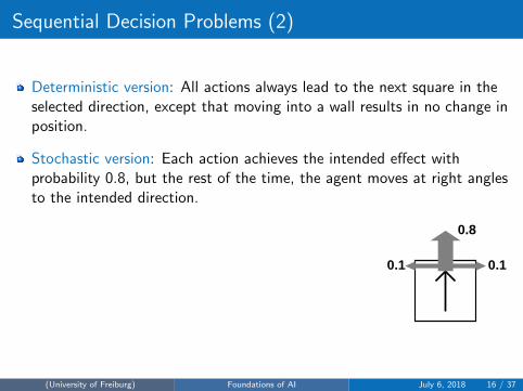
Deterministic version: All actions always lead to the next square in theselected direction, except that moving into a wall results in no change inposition.
Stochastic version: Each action achieves the intended effect withprobability 0.8, but the rest of the time, the agent moves at right anglesto the intended direction.
0.8
0.10.1
(University of Freiburg) Foundations of AI July 6, 2018 16 / 37
Lecture Overview
1 Introduction to Utility Theory
2 Choosing Individual Actions
3 Sequential Decision Problems
4 Markov Decision Processes
5 Value Iteration
(University of Freiburg) Foundations of AI July 6, 2018 17 / 37
Markov Decision Problem (MDP)
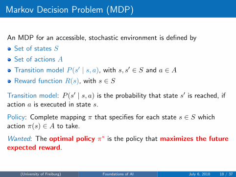
An MDP for an accessible, stochastic environment is defined by
Set of states S
Set of actions A
Transition model P (s′ | s, a), with s, s′ ∈ S and a ∈ AReward function R(s), with s ∈ S
Transition model: P (s′ | s, a) is the probability that state s′ is reached, ifaction a is executed in state s.
Policy: Complete mapping π that specifies for each state s ∈ S whichaction π(s) ∈ A to take.
Wanted: The optimal policy π∗ is the policy that maximizes the futureexpected reward.
(University of Freiburg) Foundations of AI July 6, 2018 18 / 37
Optimal Policies (1)
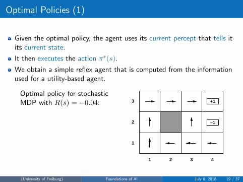
Given the optimal policy, the agent uses its current percept that tells itits current state.
It then executes the action π∗(s).
We obtain a simple reflex agent that is computed from the informationused for a utility-based agent.
Optimal policy for stochasticMDP with R(s) = −0.04:
–1
+1
1
2
3
1 2 3 4
(University of Freiburg) Foundations of AI July 6, 2018 19 / 37
Optimal Policies (2)
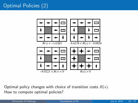
Optimal policy changes with choice of transition costs R(s).How to compute optimal policies?
(University of Freiburg) Foundations of AI July 6, 2018 20 / 37
Finite and Infinite Horizon Problems
Performance of the agent is measured by the sum of rewards for thestates visited.
To determine an optimal policy we will first calculate the utility of eachstate and then use the state utilities to select the optimal action foreach state.
The result depends on whether we have a finite or infinite horizonproblem.
Utility function for state sequences: Uh([s0, s1, . . . , sn])
For finite horizon problems the optimal policy depends on the currentstate and the remaining steps to go. It therefore depends on time and iscalled nonstationary.
In infinite horizon problems the optimal policy only depends on thecurrent state and therefore is stationary.
(University of Freiburg) Foundations of AI July 6, 2018 21 / 37
Assigning Utilities to State Sequences
For stationary systems there are two coherent ways to assign utilities tostate sequences.
The term γ ∈ [0, 1[ is called the discount factor.
With discounted rewards the utility of an infinite state sequence isalways finite. The discount factor expresses that future rewards haveless value than current rewards.
(University of Freiburg) Foundations of AI July 6, 2018 22 / 37
Lecture Overview
1 Introduction to Utility Theory
2 Choosing Individual Actions
3 Sequential Decision Problems
4 Markov Decision Processes
5 Value Iteration
(University of Freiburg) Foundations of AI July 6, 2018 23 / 37
Utilities of States
The utility of a state depends on the utility of the state sequences thatfollow it.
Let Uπ(s) be the utility of a state under policy π.
Let st be the state of the agent after executing π for t steps. Thus, theutility of s under π is
Uπ(s) = E
[ ∞∑t=0
γtR(st) | π, s0 = s
]
The true utility U(s) of a state is Uπ∗(s).
R(s) is the short-term reward for being in s andU(s) is the long-term total reward from s onwards.
(University of Freiburg) Foundations of AI July 6, 2018 24 / 37
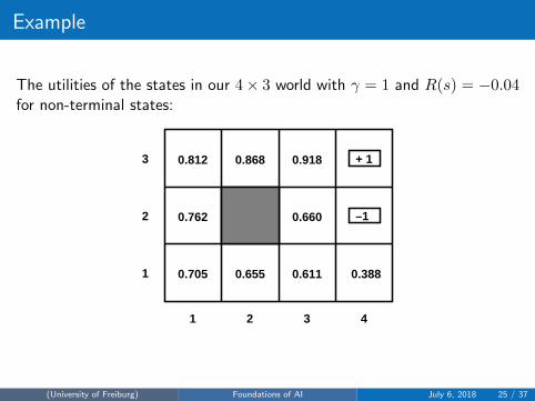
Example
The utilities of the states in our 4× 3 world with γ = 1 and R(s) = −0.04for non-terminal states:
1 2 3
1
2
3
–1
+ 1
4
0.611
0.812
0.655
0.762
0.918
0.705
0.660
0.868
0.388
(University of Freiburg) Foundations of AI July 6, 2018 25 / 37
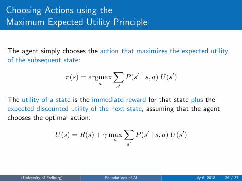
Choosing Actions using theMaximum Expected Utility Principle
The agent simply chooses the action that maximizes the expected utilityof the subsequent state:
π(s) = argmaxa
∑s′
P (s′ | s, a) U(s′)
The utility of a state is the immediate reward for that state plus theexpected discounted utility of the next state, assuming that the agentchooses the optimal action:
U(s) = R(s) + γmaxa
∑s′
P (s′ | s, a) U(s′)
(University of Freiburg) Foundations of AI July 6, 2018 26 / 37
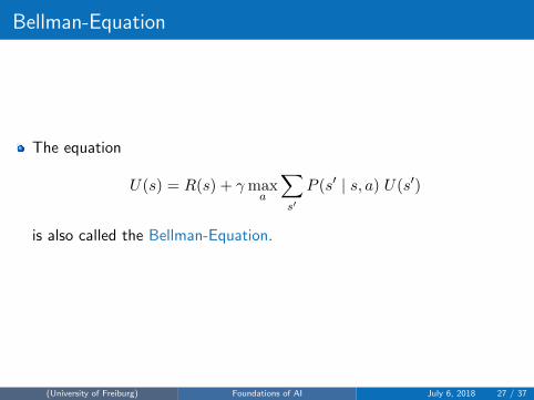
Bellman-Equation
The equation
U(s) = R(s) + γmaxa
∑s′
P (s′ | s, a) U(s′)
is also called the Bellman-Equation.
(University of Freiburg) Foundations of AI July 6, 2018 27 / 37
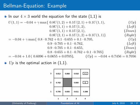
Bellman-Equation: Example
In our 4× 3 world the equation for the state (1,1) is
(University of Freiburg) Foundations of AI July 6, 2018 28 / 37
Value Iteration (1)
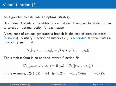
An algorithm to calculate an optimal strategy.
Basic Idea: Calculate the utility of each state. Then use the state utilitiesto select an optimal action for each state.
A sequence of actions generates a branch in the tree of possible states(histories). A utility function on histories Uh is separable iff there exists afunction f such that
In the example, R((4, 3)) = +1, R((4, 2)) = −1, R(other) = −1/25.
(University of Freiburg) Foundations of AI July 6, 2018 29 / 37
Value Iteration (2)
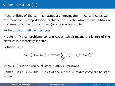
If the utilities of the terminal states are known, then in certain cases wecan reduce an n-step decision problem to the calculation of the utilities ofthe terminal states of the (n− 1)-step decision problem.
→ Iterative and efficient process
Problem: Typical problems contain cycles, which means the length of thehistories is potentially infinite.
Solution: Use
Ut+1(s) = R(s) + γmaxa
∑s′
P (s′ | s, a) Ut(s′)
where Ut(s) is the utility of state s after t iterations.
Remark: As t→∞, the utilities of the individual states converge to stablevalues.
(University of Freiburg) Foundations of AI July 6, 2018 30 / 37
Value Iteration (3)
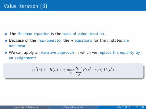
The Bellman equation is the basis of value iteration.
Because of the max-operator the n equations for the n states arenonlinear.
We can apply an iterative approach in which we replace the equality byan assignment:
U ′(s)← R(s) + γmaxa
∑s′
P (s′ | s, a) U(s′)
(University of Freiburg) Foundations of AI July 6, 2018 31 / 37
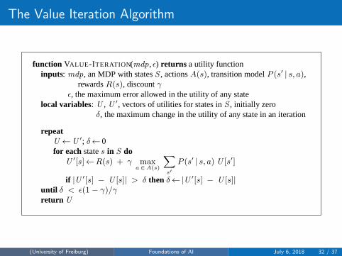
The Value Iteration Algorithm
17 MAKING COMPLEXDECISIONS
function VALUE -ITERATION(mdp,ǫ) returns a utility functioninputs: mdp, an MDP with statesS , actionsA(s), transition modelP (s′ | s, a),
rewardsR(s), discountγǫ, the maximum error allowed in the utility of any state
local variables: U , U ′, vectors of utilities for states inS , initially zeroδ, the maximum change in the utility of any state in an iteration
repeatU ←U ′; δ← 0for each states in S do
U ′[s]←R(s) + γ maxa∈A(s)
X
s′P (s′ | s, a) U [s′]
if |U ′[s] − U [s]| > δ then δ←|U ′[s] − U [s]|until δ < ǫ(1− γ)/γreturn U
Figure 17.4 The value iteration algorithm for calculating utilities ofstates. The termination condi-tion is from Equation (??).
39
(University of Freiburg) Foundations of AI July 6, 2018 32 / 37
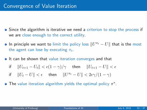
Convergence of Value Iteration
Since the algorithm is iterative we need a criterion to stop the process ifwe are close enough to the correct utility.
In principle we want to limit the policy loss ‖Uπt − U‖ that is the mostthe agent can lose by executing πt.
It can be shown that value iteration converges and that
if ‖Ut+1 − Ut‖ < ε(1− γ)/γ then ‖Ut+1 − U‖ < ε
if ‖Ut − U‖ < ε then ‖Uπt − U‖ < 2εγ/(1− γ)
The value iteration algorithm yields the optimal policy π∗.
(University of Freiburg) Foundations of AI July 6, 2018 33 / 37
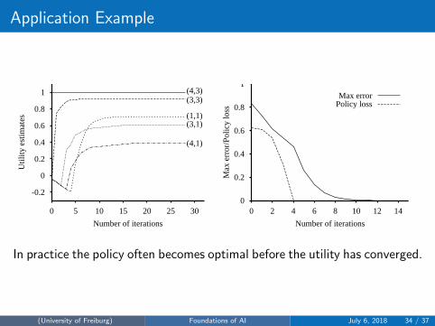
Application Example
-0.2
0
0.2
0.4
0.6
0.8
1
0 5 10 15 20 25 30
Util
ity e
stim
ates
Number of iterations
(4,3)(3,3)
(1,1)(3,1)
(4,1)
0
0.2
0.4
0.6
0.8
1
0 2 4 6 8 10 12 14
Max
err
or/P
olic
y lo
ssNumber of iterations
Max errorPolicy loss
In practice the policy often becomes optimal before the utility has converged.
(University of Freiburg) Foundations of AI July 6, 2018 34 / 37
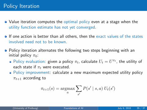
Policy Iteration
Value iteration computes the optimal policy even at a stage when theutility function estimate has not yet converged.
If one action is better than all others, then the exact values of the statesinvolved need not to be known.
Policy iteration alternates the following two steps beginning with aninitial policy π0:
Policy evaluation: given a policy πt, calculate Ut = Uπt , the utility ofeach state if πt were executed.Policy improvement: calculate a new maximum expected utility policyπt+1 according to
πt+1(s) = argmaxa
∑s′
P (s′ | s, a) Ut(s′)
(University of Freiburg) Foundations of AI July 6, 2018 35 / 37
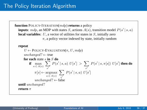
The Policy Iteration Algorithm
40 Chapter 17. Making Complex Decisions
function POLICY-ITERATION(mdp) returns a policyinputs: mdp, an MDP with statesS , actionsA(s), transition modelP (s′ | s, a)local variables: U , a vector of utilities for states inS , initially zero
π, a policy vector indexed by state, initially random
repeatU ← POLICY-EVALUATION (π,U ,mdp)unchanged?← truefor each states in S do
if maxa∈A(s)
X
s′P (s′ | s, a) U [s′] >
X
s′P (s′ | s, π[s]) U [s′] then do
π[s]← argmaxa∈A(s)
X
s′P (s′ | s, a) U [s′]
unchanged?← falseuntil unchanged?return π
Figure 17.7 The policy iteration algorithm for calculating an optimal policy.
function POMDP-VALUE -ITERATION(pomdp,ǫ) returns a utility functioninputs: pomdp, a POMDP with statesS , actionsA(s), transition modelP (s′ | s, a),
sensor modelP (e | s), rewardsR(s), discountγǫ, the maximum error allowed in the utility of any state
local variables: U , U ′, sets of plansp with associated utility vectorsαp
U ′←a set containing just the empty plan[ ], with α[ ](s)= R(s)repeat
U ←U ′
U ′← the set of all plans consisting of an action and, for each possible next percept,a plan inU with utility vectors computed according to Equation (??)
U ′←REMOVE-DOMINATED-PLANS(U ′)until MAX -DIFFERENCE(U ,U ′) < ǫ(1− γ)/γreturn U
Figure 17.9 A high-level sketch of the value iteration algorithm for POMDPs. TheREMOVE-DOMINATED-PLANS step and MAX -DIFFERENCEtest are typically implemented as linearprograms.
(University of Freiburg) Foundations of AI July 6, 2018 36 / 37
Summary
Rational agents can be developed on the basis of a probability theoryand a utility theory.
Agents that make decisions according to the axioms of utility theorypossess a utility function.
Sequential problems in uncertain environments (MDPs) can be solvedby calculating a policy.
Value iteration is a process for calculating optimal policies.
(University of Freiburg) Foundations of AI July 6, 2018 37 / 37