Comparison of arti cial neural network and coupled...

Scientia Iranica A (2017) 24(2), 487{496

Sharif University of TechnologyScientia Iranica

Transactions A: Civil Engineeringwww.scientiairanica.com

Comparison of arti�cial neural network and coupledsimulated annealing based least square support vectorregression models for prediction of compressivestrength of high-performance concrete

M.A. Ayubi Rada;� and M.S. Ayubi Radb

a. Advanced Control Systems Lab (ACSL), Control & Intelligent Processing Center of Excellence, University of Tehran, NorthKargar Ave, Tehran, P.O. Box 14395/515, Iran.

b. Department of Civil and Environmental Engineering, Shiraz University, Molla Sadra St., Shiraz, Fars, P.O. Box 71348-51154,Iran.

Received 19 April 2015; received in revised form 30 November 2015; accepted 27 February 2016

KEYWORDSHigh performanceconcrete;Compressive strength;Coupled simulatedannealing;ANN;LSSVR.

Abstract. High-Performance Concrete (HPC) is a complex composite material withhighly nonlinear mechanical behavior. Concrete compressive strength, as one of themost essential qualities of concrete, is also a highly nonlinear function of ingredients. Inthis paper, Least Square Support Vector Regression (LSSVR) model based on CoupledSimulated Annealing (CSA) has been successfully used to �nd the nonlinear relationshipbetween the concrete compressive strength and eight input factors (the cement, the blastfurnace slags, the y ashes, the water, the superplasticizer, the coarse aggregates, the �neaggregates, age of testing). To evaluate the performance of the CSA-LSSVR model, theresults of the hybrid model were compared with those obtained by Arti�cial Neural Network(ANN) model. A comparison study is made using the coe�cient of determination R2 andRoot Mean Squared Error (RMSE) as evaluation criteria. The accuracy, the computationaltime, the advantages and shortcomings of these modeling methods are also discussed. Thetraining and testing results have shown that ANNs and CSA-LSSVR models have strongpotential for predicting the compressive strength of HPC.© 2017 Sharif University of Technology. All rights reserved.

1. Introduction

High-performance concrete is a construction materialcharacterized by high workability, high strength, andhigh durability. The American Concrete Institute(ACI) de�nes HPC as concrete meeting special com-bination of performance and uniformity requirementsthat cannot always be achieved routinely using con-ventional constituents and normal mixing, placing, and

*. Corresponding author. Tel.: +98 711 7137315833;Fax: +98 21 61119742Email addresses: [email protected] (M.A. Ayubi Rad);[email protected] (M.S. Ayubi Rad)

curing practices [1]. The conventional concrete is amixture of water, Portland cement, �ne aggregate, andcoarse aggregate, while HPC employs y ash, blastfurnace slag, and silica fume as mineral admixtures,and superplasticizer as chemical admixture [2,3]. Theuse of mineral admixtures as partial cement replace-ment improves the properties of concrete by actingas �ne �llers and pozzolanic materials [2]. On theother hand, the chemical admixture improves thecompressive strength of HPC by reducing the watercontent and the level of porosity within the hydratedcement paste [3,4].

The compressive strength is a major mechanicalproperty and probably the most essential quality of

488 M.A. Ayubi Rad and M.S. Ayubi Rad/Scientia Iranica, Transactions A: Civil Engineering 24 (2017) 487{496

concrete which is generally obtained by measuringthe concrete specimen after a standard curing of 28days [5], but waiting 28 days to get the 28-day com-pressing strength is time-consuming and uncommon.Therefore, designing a prediction model to obtain anearly determination of compressive strength has gaineda lot of attention.

For conventional concrete, the linear and nonlin-ear regression models can be used to predict the valuesof compressive strength, but for HPC as the numberof input factor increases, the relationship between theinput factors and the compressive strength becomeshighly nonlinear and complex. Hence, the regressionmodels are not suitable for predicting the values ofcompressive strength of HPC [6]. Therefore, moreattentions have been paid to models based on arti�cialintelligence. Yeh [7] proposed a novel neural networkarchitecture and examined its e�ciency and accuracyin modeling the compressive strength of concrete.Prasad et al. [8] used an ANN to predict the 28-daycompressive strength of a normal and high strengthSelf-Compacting Concrete (SCC) and HPC with highvolume y ash. Sobhani et al. [9] proposed severalregression models, Adaptive Neuro Fuzzy InferenceSystem (ANFIS), and ANN model to predict the 28-day compressive strength of no-slump concrete. Theyshowed that the neural network and ANFIS modelscan predict the compressive strength with satisfactoryperformance, but the regression models fail to bereliable. Alshihri et al.[10] investigated the use ofBack-Propagation (BP) and Cascade Correlation (CC)neural networks for predicting the compressive strengthof Light Weight Concrete (LWC). The �ndings of theirstudy indicated that the neural network models aresu�cient tools for predicting the compressive strengthof LWC. Topcu and Sar�demir [11] developed ANN andfuzzy logic models for predicting 7, 28, and 90 dayscompressive strength of concretes containing high-limeand low-lime y ashes. Their conclusions have shownthat ANN and fuzzy logic models are practical modelsfor predicting the compressive strength of concrete.Cheng et al. [6] proposed an arti�cial intelligencehybrid system to predict the HPC compressive strengthby fusing the fuzzy logic, weighted Support Vector Ma-chines (SVMs), and fast messy genetic algorithm intoEvolutionary Fuzzy Support Vector Machine InferenceModel for Time Series Data (EFSIMT). Their valida-tion results indicated that EFSIMT method achieveshigher performance goal in comparison with SVMs.They also concluded that in comparison with ANN andEFSIMT, the SVMs have the least satisfactory result.

The aim of this study is to improve the accuracyof SVM model in predicting the compressive strengthof HPC. In spite of SVM's many advantages, thetheory of SVM only covers the determination of theparameters for a given value of the regularization and

kernel parameters and choice of kernel. The existingSVM methods also have high algorithmic complexityand extensive memory requirements. In this paper,the LSSVR model, a variation of Support VectorRegression (SVR) model with lower computationalcost, has been proposed. However, similar to SVR,the e�ectiveness of the LSSVR model depends onthe appropriate regularization and kernel parametersettings which can be identi�ed as an optimizationproblem. In this work, the CSA [12], as a globaloptimization method, has been used for determiningthe tuning parameters of LSSVR model. The proposedmodel is constructed, trained, tested, and validatedby applying the HPC experimental data originallygenerated by Yeh [13]. It is shown that in comparisonwith ANN, in terms of accuracy, the proposed CSA-LSSVR method achieves comparable results.

2. Data collection

The experimental datasets were obtained from Univer-sity of California, Irvine (UCI) database, provided byProfessor Yeh [13]. The dataset is consisted of 1030samples, each containing 8 components for input vectorand one output value (compressive strength). To buildand evaluate the model, we used random sampling andgenerated 4 datasets and named them Experiment 1,Experiment 2, Experiment 3, and Experiment 4. Eachgenerated dataset was divided into two categories. 800samples were used for training and 230 samples wereused to evaluate the ANN and CSA-LSSVR models.Table 1 shows the experimental data used in this study.Table 2 presents the range of inputs and outputs.

3. Arti�cial neural network model

ANNs are computational models which were developedto mimic the biological neural networks. ANNs havebeen used by many researchers for a variety of di�erentapplications [14,15]. In civil engineering, the ANNshave been applied to damage detection of bridgestructures [16], modeling the mechanical behavior ofmaterials [17], active control of structures [18], optimalmonitoring network of ground water [19], and concretemix proportion design [20]. An arti�cial neuron isconsisted of 5 major units: inputs, weights, sumfunction, activation function, and outputs. The inputsto the network are represented by x = (x0; x1; :::; xn)where x0 is a constant. Each input is multiplied bya connection weight. The weights are represented byw = (w0; w1; :::; wn). The weighted sum of inputs iscalculated as follows:

(net)j =nXi=0

wijxi; (1)

M.A. Ayubi Rad and M.S. Ayubi Rad/Scientia Iranica, Transactions A: Civil Engineering 24 (2017) 487{496 489

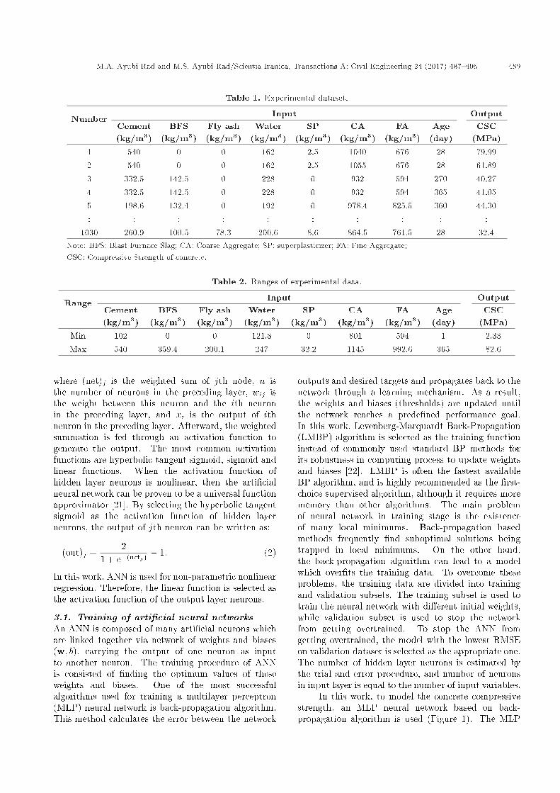
Table 1. Experimental dataset.

Number Input OutputCement(kg/m3)

BFS(kg/m3)

Fly ash(kg/m3)

Water(kg/m3)

SP(kg/m3)

CA(kg/m3)

FA(kg/m3)

Age(day)

CSC(MPa)

1 540 0 0 162 2.5 1040 676 28 79.992 540 0 0 162 2.5 1055 676 28 61.893 332.5 142.5 0 228 0 932 594 270 40.274 332.5 142.5 0 228 0 932 594 365 41.055 198.6 132.4 0 192 0 978.4 825.5 360 44.30: : : : : : : : : :

1030 260.9 100.5 78.3 200.6 8.6 864.5 761.5 28 32.4Note: BFS: Blast Furnace Slag; CA: Coarse Aggregate; SP: superplasticizer; FA: Fine Aggregate;CSC: Compressive Strength of concrete.

Table 2. Ranges of experimental data.

Range Input OutputCement(kg/m3)

BFS(kg/m3)

Fly ash(kg/m3)

Water(kg/m3)

SP(kg/m3)

CA(kg/m3)

FA(kg/m3)

Age(day)

CSC(MPa)

Min 102 0 0 121.8 0 801 594 1 2.33Max 540 359.4 200.1 247 32.2 1145 992.6 365 82.6

where (net)j is the weighted sum of jth node, n isthe number of neurons in the preceding layer, wij isthe weight between this neuron and the ith neuronin the preceding layer, and xi is the output of ithneuron in the preceding layer. Afterward, the weightedsummation is fed through an activation function togenerate the output. The most common activationfunctions are hyperbolic tangent sigmoid, sigmoid andlinear functions. When the activation function ofhidden layer neurons is nonlinear, then the arti�cialneural network can be proven to be a universal functionapproximator [21]. By selecting the hyperbolic tangentsigmoid as the activation function of hidden layerneurons, the output of jth neuron can be written as:

(out)j =2

1 + e�(netj)� 1: (2)

In this work, ANN is used for non-parametric nonlinearregression. Therefore, the linear function is selected asthe activation function of the output layer neurons.

3.1. Training of arti�cial neural networksAn ANN is composed of many arti�cial neurons whichare linked together via network of weights and biases(w; b), carrying the output of one neuron as inputto another neuron. The training procedure of ANNis consisted of �nding the optimum values of theseweights and biases. One of the most successfulalgorithms used for training a multilayer perceptron(MLP) neural network is back-propagation algorithm.This method calculates the error between the network

outputs and desired targets and propagates back to thenetwork through a learning mechanism. As a result,the weights and biases (thresholds) are updated untilthe network reaches a prede�ned performance goal.In this work, Levenberg-Marquardt Back-Propagation(LMBP) algorithm is selected as the training functioninstead of commonly used standard BP methods forits robustness in computing process to update weightsand biases [22]. LMBP is often the fastest availableBP algorithm, and is highly recommended as the �rst-choice supervised algorithm, although it requires morememory than other algorithms. The main problemof neural network in training stage is the existenceof many local minimums. Back-propagation basedmethods frequently �nd suboptimal solutions beingtrapped in local minimums. On the other hand,the back-propagation algorithm can lead to a modelwhich over�ts the training data. To overcome theseproblems, the training data are divided into trainingand validation subsets. The training subset is used totrain the neural network with di�erent initial weights,while validation subset is used to stop the networkfrom getting overtrained. To stop the ANN fromgetting overtrained, the model with the lowest RMSEon validation dataset is selected as the appropriate one.The number of hidden layer neurons is estimated bythe trial and error procedure, and number of neuronsin input layer is equal to the number of input variables.

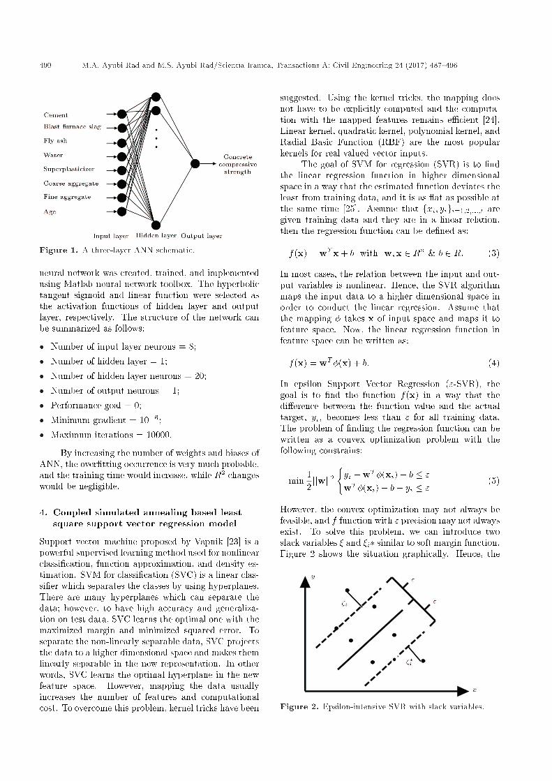
In this work, to model the concrete compressivestrength, an MLP neural network based on back-propagation algorithm is used (Figure 1). The MLP


Figure 1. A three-layer ANN schematic.

neural network was created, trained, and implementedusing Matlab neural network toolbox. The hyperbolictangent sigmoid and linear function were selected asthe activation functions of hidden layer and outputlayer, respectively. The structure of the network canbe summarized as follows:

� Number of input layer neurons = 8;� Number of hidden layer = 1;� Number of hidden layer neurons = 20;� Number of output neurons = 1;� Performance goal = 0;� Minimum gradient = 10�6;� Maximum iterations = 10000.

By increasing the number of weights and biases ofANN, the over�tting occurrence is very much probable,and the training time would increase, while R2 changeswould be negligible.

4. Coupled simulated annealing based leastsquare support vector regression model

Support vector machine proposed by Vapnik [23] is apowerful supervised learning method used for nonlinearclassi�cation, function approximation, and density es-timation. SVM for classi�cation (SVC) is a linear clas-si�er which separates the classes by using hyperplanes.There are many hyperplanes which can separate thedata; however, to have high accuracy and generaliza-tion on test data, SVC learns the optimal one with themaximized margin and minimized squared error. Toseparate the non-linearly separable data, SVC projectsthe data to a higher dimensional space and makes themlinearly separable in the new representation. In otherwords, SVC learns the optimal hyperplane in the newfeature space. However, mapping the data usuallyincreases the number of features and computationalcost. To overcome this problem, kernel tricks have been

suggested. Using the kernel tricks, the mapping doesnot have to be explicitly computed and the computa-tion with the mapped features remains e�cient [24].Linear kernel, quadratic kernel, polynomial kernel, andRadial Basic Function (RBF) are the most popularkernels for real valued vector inputs.

The goal of SVM for regression (SVR) is to �ndthe linear regression function in higher dimensionalspace in a way that the estimated function deviates theleast from training data, and it is as at as possible atthe same time [25]. Assume that fxi; yigi=1;2;:::;l aregiven training data and they are in a linear relation,then the regression function can be de�ned as:

f(x) = wTx + b with w;x 2 Rn & b 2 R: (3)

In most cases, the relation between the input and out-put variables is nonlinear. Hence, the SVR algorithmmaps the input data to a higher dimensional space inorder to conduct the linear regression. Assume thatthe mapping � takes x of input space and maps it tofeature space. Now, the linear regression function infeature space can be written as:

f(x) = wT�(x) + b: (4)

In epsilon Support Vector Regression ("-SVR), thegoal is to �nd the function f(x) in a way that thedi�erence between the function value and the actualtarget, yi, becomes less than " for all training data.The problem of �nding the regression function can bewritten as a convex optimization problem with thefollowing constrains:

min12jjwjj2

(yi �wT�(xi)� b � "wT�(xi) + b� yi � " (5)

However, the convex optimization may not always befeasible, and f function with " precision may not alwaysexist. To solve this problem, we can introduce twoslack variables � and �i� similar to soft margin function.Figure 2 shows the situation graphically. Hence, the

Figure 2. Epsilon-intensive SVR with slack variables.


convex optimization problem is reformulated as follows:

min12jjwjj2 + C

lXi=1

(�i + ��i )

8><>:yi �wT�(xi)� b � "+ �iwT�(xi) + b� yi � "+ ��i�i; ��i � 0

(6)

where C > 0 is the trade-o� between smoothness ofthe function f and the amount up to which deviationslarger than " are tolerated. In spite of SVR's manyadvantages, it still remains computationally di�cult asthe complexity of quadratic (or convex) programmingincreases with the size of dataset. LSSVR [26] simpli�esthe formulation by solving the following optimizationproblem:

min12jjwjj2 +

2

lXi=1

e2i

such that yi = wT�(xi) + b+ ei; (7)

where is the regularization parameter which deter-mines the trade-o� between the minimization of train-ing error and smoothness (or atness) of the function.By using a set of dual variables, the lagrangian functionis de�ned as follows:

L =12jjwjj2 +

2

lXi=1

e2i

�lXi=1

�i�yi �wT�(xi)� b� ei� ; (8)

where L is the Lagrangian and �i is the Lagrangemultiplier. To solve the optimization problem, thederivative of the function with respect to primal anddual variables is set as zero. As a result, we have:

@L@w

= 0! w =lXi=1

�i�(xi); (9)

@L@b

= 0!lXi=1

�i = 0; (10)

@L@ei

= 0! �i = ei; (11)

@L@�i

= 0! wT�(xi) + b+ ei � yi = 0: (12)

By substituting w and e into lagrangian, the followinglinear system is obtained [27]:�

0 1T1 + �1I

� �b�

�=�

0y

�; (13)

where:

e = [e1; e2; :::; el]T ;

� = [�1 + �2; :::; �l]T ;

= ZZT ;

Z = [�(x1); �(x2); :::; �(xl)]T ;

y = [y1; y2; :::; yl]T ;

1 = [1; 1; :::; 1]T :

The kernel trick can now be applied to forming thematrix as follows:

ij = �(xi)T�(xj) = k(xi;xj): (14)

The solution of Eq. (13) can be formulated as:

b =1T ( + �1I)�1y1T ( + �1I)�11

; (15)

� = ( + �1I)�1(y � b1): (16)

Using b and � obtained from Eqs. (15) and (16)and selecting RBF as the kernel function, the optimalregression function can be written as:

f(x) =lXi=1

�ik(xi;x) + b; (17)

k(xi;x) = exp��jjxi � xjj2

2�2

�; (18)

where �2 is called the kernel squared bandwidth. TheRBF kernel corresponds to an in�nite dimensionalfunction space. In other words, the RBF kernelde�nes a function space that is a lot larger than thatof the linear kernel or the polynomial kernel and isgenerally more exible. Model selection in LSSVR isthe major problem, because choosing the wrong kerneland regularization parameters can lead to an over�ttedmodel. As a result, the model will have low errorrate on training data and high error rate on test data.Hence, to improve the accuracy of LSSVR model, theparameters of the model should be optimized. Theparameter optimization in LSSVR model includes theregularization parameter ( ) and kernel squared band-width of RBF (�2). Previous researchers suggested


di�erent parameter settings methods for SMVs. Hsuet al. [28] suggested to set the parameters of SVM,herein and �2 to 1 and 1/k, respectively, where krepresents the number of input patterns. However,Cheng et al. [6] illustrated that this parameter settingmethod would result in a poor performance. Aiyeret al. [29] determined the parameters of LSSVM bytrial and error procedure. Since and �2 can haveany positive real values, the trial and error procedurewould be very time-consuming and often would notresult in the best parameters. In the present work,the CSA optimization method is used to optimize theparameters and �2 of LSSVR model.

4.1. Coupled simulated annealingCSA is a global optimization method based on Sim-ulated Annealing (SA) which can be used to solvea non-convex optimization problem with continuousvariables. The SA algorithm was originally inspiredfrom the annealing process which consists of heatingthe metal, holding its temperature, and then coolingit. In SA algorithm as analogous to thermodynamicannealing process, the temperature is considered as avariable. While the temperature is high, the algorithmhas the ability to jump out of any local optimumand accept solutions which are worst than the currentsolution. By reducing the temperature, the chanceof accepting worst solutions decreases. This allowsthe algorithm to focus on an area of search space inwhich near-optimum solution can be found. However,the SA algorithm is highly sensitive to the initialtemperature and the initial parameters. This promptedthe researchers to develop a new global optimizationmethod called CSA, which is consisted of several SAprocesses with coupled acceptance probabilities. Theacceptance probability of a traditional SA algorithm isoften given as:

A(x! y) =1

1 + exp�E(y)�E(x)

Tact

� ; (19)

where x and y denote the current and probing solu-tions, respectively. E(:) is the cost function and T act isthe acceptance temperature at time instant t. Whilethe acceptance probability of SA algorithm dependsonly on the current and probing solutions, the CSAalgorithm considers other current solutions coupledtogether by their cost functions, featuring a new formof acceptance probability function as follows:

A�(�; xi ! yi) =exp

�E(xi)�maxxi2�

(E(xi))

Tact

��

; (20)

and:

� =X8x2�

exp

0@E(x)� maxxi2�

(E(xi))

T act

1A ; (21)

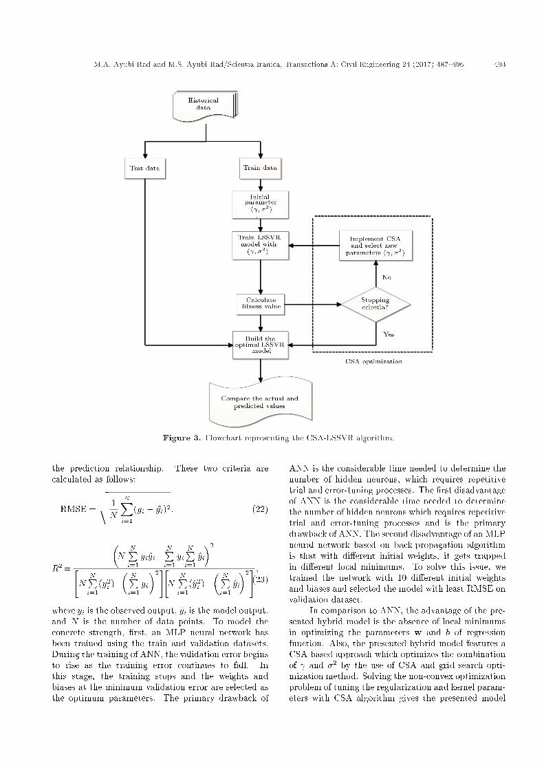
where � is the set of current states, � is the couplingterm, xi and yi, i = 1; 2; :::;m, with m being thenumber of elements in �, are the current state and thecorresponding probing state, respectively. The CSA isable to easily escape from local optima; it improves thequality of solution without slowing down the speed ofconvergence; above all, it shows an excellent reductionin dependency on initial parameters. More detailsabout the SA and CSA can be found in the paper ofXavier-de-Souza et al. [12]. The owchart of the CSA-LSSVR model is shown in Figure 3.

In this work, to optimize the parameters ofLSSVM based on CSA algorithm, we used a freelyavailable LS-SVMlab v1.8 package [30] which wasrun in Matlab commercial software. The LS-SVMlabtoolbox, �rst, uses CSA to determine the suitableparameters, then these parameters are given to a sec-ond optimization technique (simplex or grid search) toperform a �ne-tuning step. Grid search is an exhaustivesearching through a manually speci�ed subset of thehyperparameter space of a learning algorithm [31]. Toavoid over�tting, a 10-fold cross-validation algorithmis performed in the training process [32]. Note thatcompared to ANN, the LSSVR model reaches a globalminimum due to linear programming (solving a setof linear equations), but the optimization problemto be solved in tuning the kernel and regularizationparameters is generally non-convex and may have alocal minima.

5. Results and discussion

This section discusses the application of ANN andCSA-LSSVR in modeling the Compressive Strength ofConcrete (CSC) with the following eight factors:

1. Cement (kg/m3);

2. Blast furnace slag (kg/m3);

3. Fly ash (kg/m3);

4. Water (kg/m3);

5. Superplasticizer (kg/m3);

6. Coarse aggregate (kg/m3);

7. Fine aggregate (kg/m3);

8. Age (day).

RMSE and R-squared coe�cient are selected ascriteria to evaluate and compare the performance ofANN and CSA-LSSVR models. RMSE is used as ameasure of di�erences between the values predictedby the model and the values observed in the lab. R-squared is a measure of how well the independent vari-ables considered account for the measured dependentvariable [13]. The higher the R2 value, the better


Figure 3. Flowchart representing the CSA-LSSVR algorithm.

the prediction relationship. These two criteria arecalculated as follows:

RMSE =

vuut 1N

NXi=1

(yi � yi)2; (22)

R2 =

�N

NPi=1

yiyi� NPi=1

yiNPi=1

yi�2

"N

NPi=1

(y2i )�

�NPi=1

yi�2#"

NNPi=1

(y2i )�

�NPi=1

yi�2# ;

(23)

where yi is the observed output, yi is the model output,and N is the number of data points. To model theconcrete strength, �rst, an MLP neural network hasbeen trained using the train and validation datasets.During the training of ANN, the validation error beginsto rise as the training error continues to fall. Inthis stage, the training stops and the weights andbiases at the minimum validation error are selected asthe optimum parameters. The primary drawback of

ANN is the considerable time needed to determine thenumber of hidden neurons, which requires repetitivetrial and error-tuning processes. The �rst disadvantageof ANN is the considerable time needed to determinethe number of hidden neurons which requires repetitivetrial and error-tuning processes and is the primarydrawback of ANN. The second disadvantage of an MLPneural network based on back-propagation algorithmis that with di�erent initial weights, it gets trappedin di�erent local minimums. To solve this issue, wetrained the network with 10 di�erent initial weightsand biases and selected the model with least RMSE onvalidation dataset.

In comparison to ANN, the advantage of the pre-sented hybrid model is the absence of local minimumsin optimizing the parameters w and b of regressionfunction. Also, the presented hybrid model features aCSA-based approach which optimizes the combinationof and �2 by the use of CSA and grid search opti-mization method. Solving the non-convex optimizationproblem of tuning the regularization and kernel param-eters with CSA algorithm gives the presented model


Table 3. Root mean squared error of ANN and CSA-LSSVR models.

Experiment MLP CSA-LSSVRRMSE of

training datasetRMSE of

test datasetRMSE of

training datasetRMSE of

test dataset1 2.95 5.32 3.16 5.572 3.46 6.17 2.97 6.233 3.46 4.73 3.64 4.894 3.26 5.69 3.06 6.27

Table 4. The coe�cient of determination R2 of ANN and CSA-LSSVR models.

Experiment MLP CSA-LSSVRR2 of training

datasetR2 of test

datasetR2 of training

datasetR2 of test

dataset1 0.9686 0.8766 0.9644 0.88972 0.9572 0.8681 0.9688 0.86083 0.9570 0.9209 0.9541 0.91674 0.9621 0.8832 0.9668 0.8634

enormous computational advantage over other existingSVM methods. A 10-fold cross-validation method wasused to select the parameters with best cross-validationaccuracy. One fold was retained as the validationdata, while the remaining 9 folds were used as trainingdata. For dataset of Experiment 3, the parameters areselected as = 23:88 and �2 = 6:8. The performanceof ANN and CSA-LSSVR in modeling the concretecompressive strength is compared in Tables 3 and 4.

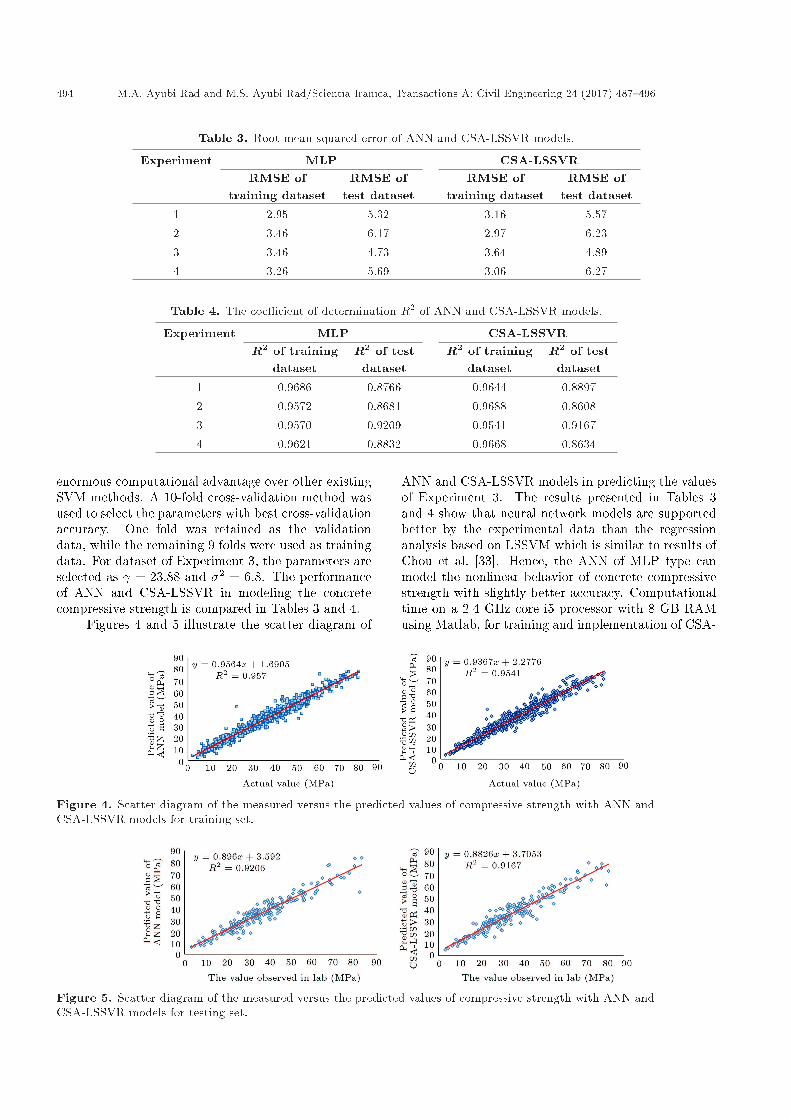
Figures 4 and 5 illustrate the scatter diagram of

ANN and CSA-LSSVR models in predicting the valuesof Experiment 3. The results presented in Tables 3and 4 show that neural network models are supportedbetter by the experimental data than the regressionanalysis based on LSSVM which is similar to results ofChou et al. [33]. Hence, the ANN of MLP type canmodel the nonlinear behavior of concrete compressivestrength with slightly better accuracy. Computationaltime on a 2.4 GHz core i5 processor with 8 GB RAMusing Matlab, for training and implementation of CSA-

Figure 4. Scatter diagram of the measured versus the predicted values of compressive strength with ANN andCSA-LSSVR models for training set.

Figure 5. Scatter diagram of the measured versus the predicted values of compressive strength with ANN andCSA-LSSVR models for testing set.


LSSVR model takes about 45.1 s and for ANN modeltakes about 495.2 s. It is because the ANN often con-verges to a local minimum, hence it has to be trainedwith di�erent initial weights, which is time-consuming.While the LSSVR models always reach the globaloptimum due to linear programming. The LSSVRmodels reduce the risk of over�tting by using thestructural risk minimization strategy, while the ANNmodels exclude or reduce this e�ect by using otherdeveloped techniques such as early stopping method.

6. Conclusions

In this study, a hybrid model was developed usinga LSSVR based on CSA optimization method forpredicting complex behavior of concrete compressivestrength. The results from the training and testingstages of the proposed hybrid model were comparedwith those obtained by ANN model using RMSE andR2 as evaluation criteria. The R-squared coe�cient fortesting set was in the range of 0.8681-0.9209 for ANNand 0.8634-0.9167 for CSA-LSSVR model. The valuesof RMSE are in range of 4.73-6.17 for ANN and 4.89-6.27 for CSA-LSSVR model in test set. The resultshave shown that in comparison with CSA-LSSVRmodel, the ANN of multilayer perceptron type canmodel the nonlinear behavior of concrete compressivestrength with slightly better accuracy. However, themajor disadvantage of ANN model was the existenceof many local minimums. As a result, di�erent initialweights would generate di�erent models with di�erentaccuracy. On the other hand, determining the numberof neurons in the hidden layer of ANN model by trialand error procedure is a time-consuming task. Whilethe CSA-LSSVR model will always converge to a globalminimum in optimizing the parameters w and b ofregression function. Also, the LSSVR model needs tooptimize only two parameters of and �2 to improveits accuracy, which gives it an enormous computationaladvantage over other methods. The weakness includesthe need for a good kernel function. The computationaltime of these two models were compared, and it wasshown that the overall training and implementationtime was less for CSA-LSSVR models than ANNs.The conclusions have shown that both ANN and CSA-LSSVR models have high potential for predicting thecompressive strength of high performance concrete.

Acknowledgment

The authors would like to thank Professor I-Cheng Yehfor providing the HPC database.

References

1. Russell, H.G. \ACI de�nes high-performance con-

crete", Concrete International, 21, pp. 56-57 (1999).

2. Bharatkumar, B., Narayanan, R., Raghuprasad, B.and Ramachandramurthy, D. \Mix proportioning ofhigh performance concrete", Cement and ConcreteComposites, 23, pp. 71-80 (2001).

3. Lim, C.-H., Yoon, Y.-S. and Kim, J.-H. \Geneticalgorithm in mix proportioning of high-performanceconcrete", Cement and Concrete Research, 34, pp.409-420 (2004).

4. A��tcin, P.-C., High Performance Concrete, CRC Press(2011).

5. Ni, H.-G. and Wang, J.-Z. \Prediction of compressivestrength of concrete by neural networks", Cement andConcrete Research, 30, pp. 1245-1250 (2000).

6. Cheng, M.-Y., Chou, J.-S., Roy, A.F. and Wu, Y.-W. \High-performance concrete compressive strengthprediction using time-weighted evolutionary fuzzy sup-port vector machines inference model", Automation inConstruction, 28, pp. 106-115 (2012).

7. Yeh, I.-C. \Modeling concrete strength with augment-neuron networks", Journal of Materials in Civil Engi-neering, 10, pp. 263-268 (1998).

8. Prasad, B.R., Eskandari, H. and Reddy, B.V. \Pre-diction of compressive strength of SCC and HPC withhigh volume y ash using ANN", Construction andBuilding Materials, 23, pp. 117-128 (2009).

9. Sobhani, J., Najimi, M., Pourkhorshidi, A.R. andParhizkar, T. \Prediction of the compressive strengthof no-slump concrete: a comparative study of regres-sion, neural network and ANFIS models", Construc-tion and Building Materials, 24, pp. 709-718 (2010).

10. Alshihri, M.M., Azmy, A.M. and El-Bisy, M.S. \Neu-ral networks for predicting compressive strength ofstructural light weight concrete", Construction andBuilding Materials, 23, pp. 2214-2219 (2009).

11. Topcu, I.B. and Sar�demir, M. \Prediction of compres-sive strength of concrete containing y ash using arti-�cial neural networks and fuzzy logic", ComputationalMaterials Science, 41, pp. 305-311 (2008).

12. Xavier-de-Souza, S., Suykens, J.A., Vandewalle, J. andBoll�e, D. \Coupled simulated annealing", Systems,Man, and Cybernetics, Part B: Cybernetics, IEEETransactions on, 40, pp. 320-335 (2010).

13. Yeh, I.-C. \Modeling of strength of high-performanceconcrete using arti�cial neural networks", Cement andConcrete Research, 28, pp. 1797-1808 (1998).

14. Rad, M.A.A. and Yazdanpanah, M.J., Designing Su-pervised Local Neural Network Classi�ers Based on EMClustering for Fault Diagnosis of Tennessee EastmanProcess, Chemometrics and Intelligent Laboratory Sys-tems (2015).

15. Rehman, A. and Saba, T. \Neural networks for docu-ment image preprocessing: state of the art", Arti�cialIntelligence Review, 42, pp. 253-273 (2014).


16. Shu, J., Zhang, Z., Gonzalez, I. and Karoumi, R.\The application of a damage detection method usingarti�cial neural network and train-induced vibrationson a simpli�ed railway bridge model", EngineeringStructures, 52, pp. 408-421 (2013).

17. El Kadi, H. \Modeling the mechanical behavior of�ber-reinforced polymeric composite materials usingarti�cial neural networks - A review", CompositeStructures, 73, pp. 1-23 (2006).

18. Ghaboussi, J. and Joghataie, A., "Active control ofstructures using neural networks", Journal of Engi-neering Mechanics, 121(4), pp. 555-567 (1995).

19. Taormina, R., Chau, K.-W. and Sethi, R. \Arti�cialneural network simulation of hourly groundwater levelsin a coastal aquifer system of the Venice lagoon",Engineering Applications of Arti�cial Intelligence, 25,pp. 1670-1676 (2012).

20. Ji, T., Lin, T. and Lin, X. \A concrete mix proportiondesign algorithm based on arti�cial neural networks",Cement and Concrete Research, 36, pp. 1399-1408(2006).

21. Hornik, K. \Approximation capabilities of multilayerfeedforward networks", Neural Networks, 4, pp. 251-257 (1991).

22. Suratgar, A.A., Tavakoli, M.B. and Hoseinabadi, A.\Modi�ed Levenberg-Marquardt method for neuralnetworks training", World Acad. Sci. Eng. Technol, 6,pp. 46-48 (2005).

23. Cortes, C. and Vapnik, V. \Support-vector networks",Machine Learning, 20, pp. 273-297 (1995).

24. Press, W.H., Numerical Recipes 3rd Edition: The Artof Scienti�c Computing: Cambridge University Press(2007).

25. Smola, A.J. and Sch�olkopf, B. \A tutorial on supportvector regression", Statistics and Computing, 14, pp.199-222 (2004).

26. Suykens, J.A., Van Gestel, T., De Moor, B. and Van-dewalle, J., Least Squares Support Vector Machines, 4,World Scienti�c (2002).

27. Guo, Z. and Bai, G. \Application of least squaressupport vector machine for regression to reliabilityanalysis", Chinese Journal of Aeronautics, 22, pp. 160-166 (2009).

28. Hsu, C.W., Chang, C.C. and Lin, C.J., A PracticalGuide to Support Vector Classi�cation, Department ofComputer Science, Taipei 106, Taiwan (2003).

29. Aiyer, B.G., Kim, D., Karingattikkal, N., Samui, P.and Rao, P.R. \Prediction of compressive strength ofself-compacting concrete using least square supportvector machine and relevance vector machine", KSCEJournal of Civil Engineering, 18, pp. 1753-1758 (2014).

30. http://www.esat.kuleuven.be/sista/lssvmlab/.

31. Bergstra, J. and Bengio, Y. \Random search for hyper-parameter optimization", The Journal of MachineLearning Research, 13, pp. 281-305 (2012).

32. Chou, J.-S. and Pham, A.-D. \Hybrid computationalmodel for predicting bridge scour depth near piers andabutments", Automation in Construction, 48, pp. 88-96 (2014).

33. Chou, J.-S., Chiu, C.-K., Farfoura, M. and Al-Taharwa, I. \Optimizing the prediction accuracy ofconcrete compressive strength based on a comparisonof data-mining techniques", Journal of Computing inCivil Engineering, 25, pp. 242-253 (2010).

Biographies

Mostafa Ali Ayubi Rad received his BS degreein Electrical Engineering from Shiraz University ofTechnology, Shiraz, Iran, in 2012, and his MS degreefrom University of Tehran, Iran, in 2015. His �eld ofresearch includes engineering applications of arti�cialintelligence and application of various nonlinear con-trollers on power converters.

Mohammad Sadegh Ayubi Rad is a PhD studentin Department of Civil and Environmental Engineeringat Shiraz University, Shiraz, Iran. He holds BS degreein Civil Engineering from Shahid Bahonar University ofKerman, Kerman, Iran, and MS degree from MalayerUniversity, Malayer, Iran. His research interests in-clude structural optimization, reliability-based design,and seismic design of structures.

Date post:	06-May-2019
Category:	Documents
Upload:	dangnga
View:	226 times
Download:	0 times

Comparison of arti cial neural network and coupled...

Documents