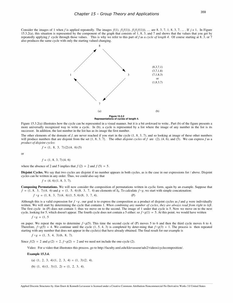
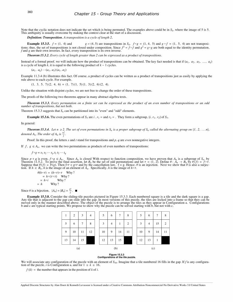
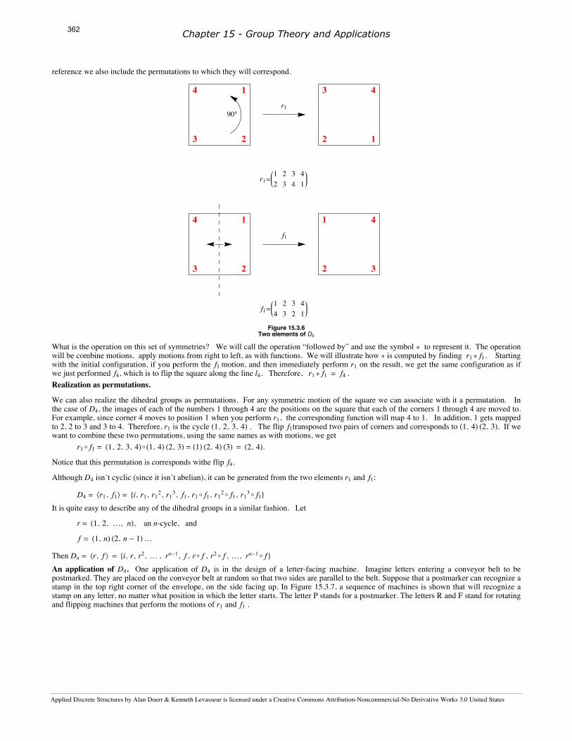
Applied Discrete Structures - University of Massachusetts Lowell

Applied Discrete Structures

Algebraic StructuresChapters 11-16

Alan Doerr and Kenneth LevasseurDepartment Of Mathematical Sciences

University of Massachusetts Lowell

Version 1.01 July 2012

Home Blog Errata

Home: http://faculty.uml.edu/klevasseur/ADS2/”Blog: http://applieddiscretestructures.blogspot.com/

Errata: http://faculty.uml.edu/klevasseur/ADS2/errata.html

Applied Discrete Structures by Alan Doerr & Kenneth Levasseur is licensed under a Creative Commons Attribution-Noncommercial-ShareA-like 3.0 United States License.(http://creativecommons.org/licenses/by-nc-sa/3.0/us/)

Previously published by Pearson Education, Inc. under the title Applied Discrete Structures for Computer Science

To our families Donna, Christopher, Melissa, and Patrick Doerr

and Karen, Joseph, Kathryn, and Matthew Levasseur


Applied Discrete Structures by Alan Doerr & Kenneth Levasseur is licensed under a Creative Commons Attribution-Noncommercial-No Derivative Works

Table of ContentsPreface

Chapter 11 AlgebraIc Systems11.1 Operations11.2 Algebraic Systems11.3 Some General Properties of Groups11.4 Zn, the Integers Modulo n11.5 Subsystems11.6 Direct Products11.7 Isomorphisms11.8 Using Computers to Study GroupsSupplementary Exercises for Chapter 11

Chapter 12 More Matrix Algebra12.1 Systems of Linear Equations12.2 Matrix Inversion12.3 An Introduction to Vector Spaces12.4 The Diagonialization Process12.5 Some ApplicationsSupplementary Exercises for Chapter 12

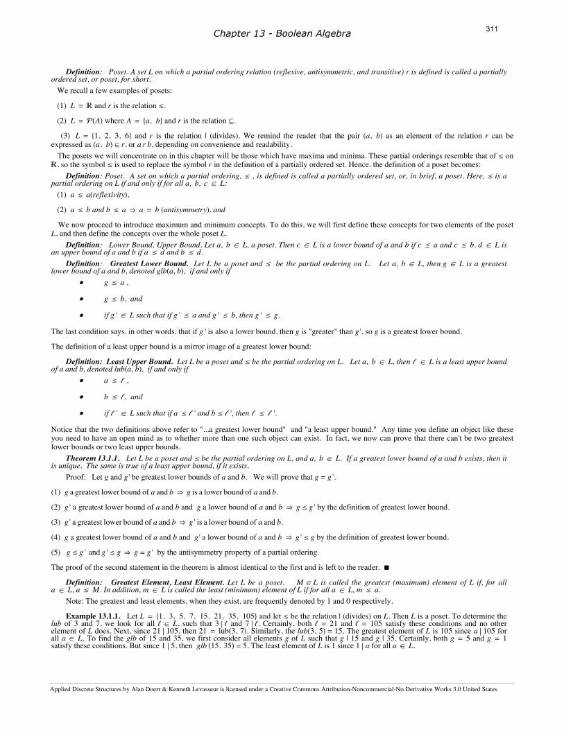
Chapter 13 Boolean Algebra13.1 Posets Revisited13.2 Lattices13.3 Boolean Algebras13.4 Atoms of a Boolean Algebra13.5 Finite Boolean Algebras as n-tuples of Zeros and Ones13.6 Boolean Expressions13.7 A Brief Introduction to the Application of Boolean Algebra to Switching TheorySupplementary Exercises for Chapter 13

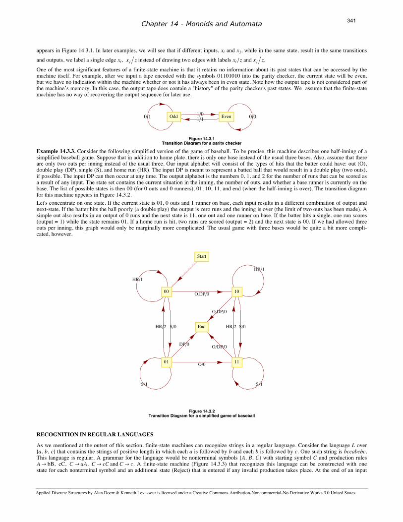
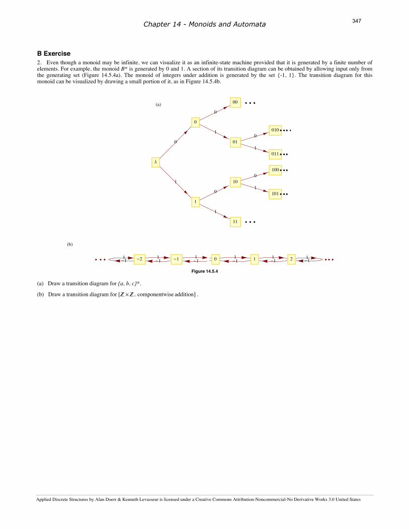
Chapter 14 Monoids and Automata14.1 Monoids14.2 Free Monoids and Languages14.3 Automata, Finite-state Machines14.4 The Monoid of A Finite-state Machine14.5 The Machine of A MonoidSupplementary Exercises for Chapter 14

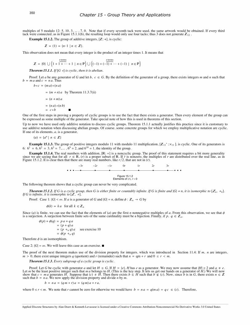
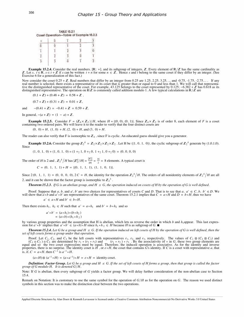
Chapter 15 Groups Theory and Applications15.1 Cyclic Groups15.2 Cosets and Factor Groups



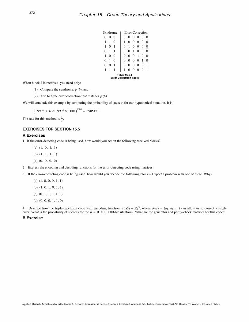
p15.3 Permutation Groups15.4 Normal Subgroups and Group Homomorphisms15.5 Coding Theory—Group CodesSupplementary Exercises for Chapter 15

Chapter 16 An Introduction to Rings and Fields16.1 Rings—Basic Definitions and Concepts16.2 Fields16.3 Polynomial Rings16.4 Field Extensions16.5 Power SeriesSupplementary Exercises for Chapter 16

Solutions and Hints to Selected Exercises

Back Matter



Preface - what a difference 21 years make!This is Applied Discrete Structures, Part II - Algebraic Structures, which contains an introduction to groups, monoids, rings, fields,vectorspaces, lattices, and boolean algebras. It corresponds with the content of Discrete Structures II at UMass Lowell, which is a required coursefor students in Computer Science. It presumes background contained in Part I - Fundamentals, which is the content of Discrete Structures Iat UMass Lowell.

Twenty-one years after the publication of the 2nd edition of Applied Discrete Structures for Computer Science, in 1989 the publishing andcomputing landscape have both changed dramatically. We signed a contract for the second edition with Science Research Associates but by thetime the book was ready to print, SRA had been sold to MacMillan. Soon after, the rights had been passed on to Pearson Education, Inc. In2010, the long-term future of printed textbooks is uncertain. In the meantime, textbook prices (both printed and e-books) have increased and agrowing open source textbook market movement has started. One of our objectives in revisiting this text is to make it available to our studentsin an affordable format. In its original form, the text was peer-reviewed and was adopted for use at several universities throughout the country.For this reason, we see Applied Discrete Structures as not only an inexpensive alternative, but a high quality alternative. As indicated above the computing landscape is very different from the 1980's and accounts for the most significant changes in the text. One ofthe most common programming languages of the 1980's, Pascal; and we used it to illustrate many of the concepts in the text. Although it isn'ttotally dead, Pascal is far from the mainstream of computing in the 21st century. In 1989, Mathematica had been out for less than a year —now a major force in scientific computing. The open source software movement also started in the 1980's and in 2005, the first version ofSage, an open-source alternative to Mathematica was first released. In Applied Discrete Structures we have replaced "Pascal Notes" with"Mathematica Notes" and "Sage Notes." Finally, 1989 was the year that World Wide Web was invented by Tim Berners-Lee. There wasn't asingle www in the 2nd edition. In this version, we intend to make use of extensive web resources, including video demonstrations.We would like to thank Tony Penta, Sitansu Mittra, and Dan Klain for using the preliminary versions of Applied Discrete Structures. Thecorrections and input they provided was appreciated.We repeat the preface to Applied Discrete Structures for Computer Science below. Plans for the instructor's guide, which is mentioned in thepreface are uncertain at this time.

Preface to Applied Discrete Structures for Computer Science, 2nd Ed.

We feel proud and fortunate that most authorities, including MAA and ACM, have settled on a discrete mathematics syllabus that is virtuallyidentical to the contents of the first edition of Applied Discrete Structures for Computer Science. For that reason, very few topical changesneeded to be made in this new edition, and the order of topics is almost unchanged. The main change is the addition of a large number ofexercises at all levels. We have "fine-tuned" the contents by expanding the preliminary coverage of sets and combinatorics, and we have addeda discussion of binary integer representation. We have also added an introduction including several examples, to provide motivation for thosestudents who may find it reassuring to know that mathematics has "real" applications. "Appendix B—Introduction to Algorithms," has alsobeen added to make the text more self-contained.

How This Book Will Help StudentsIn writing this book, care was taken to use language and examples that gradually wean students from a simpleminded mechanical approach andmove them toward mathematical maturity. We also recognize that many students who hesitate to ask for help from an instructor need a readabletext, and we have tried to anticipate the questions that go unasked.The wide range of examples in the text are meant to augment the "favorite examples" that most instructors have for teaching the topics indiscrete mathematics.To provide diagnostic help and encouragement, we have included solutions and/or hints to the odd-numbered exercises. These solutions includedetailed answers whenever warranted and complete proofs, not just terse outlines of proofs.Our use of standard terminology and notation makes Applied Discrete Structures for Computer Science a valuable reference book for futurecourses. Although many advanced books have a short review of elementary topics, they cannot be complete.

How This Book Will Help InstructorsThe text is divided into lecture-length sections, facilitating the organization of an instructor's presentation.

Topics are presented in such a way that students' understanding can be monitored through thought-provoking exercises. The exercises requirean understanding of the topics and how they are interrelated, not just a familiarity with the key words.An Instructor's Guide is available to any instructor who uses the text. It includes:

(a) Chapter-by-chapter comments on subtopics that emphasize the pitfalls to avoid;

(b) Suggested coverage times;

(c) Detailed solutions to most even-numbered exercises;

(d) Sample quizzes, exams, and final exams.



How This Book Will Help the Chairperson/CoordinatorThe text covers the standard topics that all instructors must be aware of; therefore it is safe to adopt Applied Discrete Structures for ComputerScience before an instructor has been selected.The breadth of topics covered allows for flexibility that may be needed due to last-minute curriculum changes.

Since discrete mathematics is such a new course, faculty are often forced to teach the course without being completely familiar with it. AnInstructor's Guide is an important feature for the new instructor.

What a Difference Five Years Makes!In the last five years, much has taken place in regards to discrete mathematics. A review of these events is in order to see how they haveaffected the Second Edition of Applied Discrete Structures for Computer Science.(1) Scores of discrete mathematics texts have been published. Most texts in discrete mathematics can be classified as one-semester or two-semester texts. The two-semester texts, such as Applied Discrete Structures for Computer Science, differ in that the logical prerequisites for amore thorough study of discrete mathematics are developed.(2) Discrete mathematics has become more than just a computer science support course. Mathematics majors are being required to take it, oftenbefore calculus. Rather than reducing the significance of calculus, this recognizes that the material a student sees in a discrete mathematics/struc-tures course strengthens his or her understanding of the theoretical aspects of calculus. This is particularly important for today's students, sincemany high school courses in geometry stress mechanics as opposed to proofs. The typical college freshman is skill-oriented and does not have ahigh level of mathematical maturity. Discrete mathematics is also more typical of the higher-level courses that a mathematics major is likely totake.(3) Authorities such as MAA, ACM, and A. Ralson have all refined their ideas of what a discrete mathematics course should be. Instead of thechaos that characterized the early '80s, we now have some agreement, namely that discrete mathematics should be a course that developsmathematical maturity.(4) Computer science enrollments have leveled off and in some cases have declined. Some attribute this to the lay-offs that have taken place inthe computer industry; but the amount of higher mathematics that is needed to advance in many areas of computer science has also discouragedmany. A year of discrete mathematics is an important first step in overcoming a deficiency in mathematics.(5) The Educational Testing Service introduced its Advanced Placement Exam in Computer Science. The suggested preparation for this examincludes many discrete mathematics topics, such as trees, graphs, and recursion. This continues the trend toward offering discrete mathematicsearlier in the overall curriculum.

AcknowledgmentsThe authors wish to thank our colleagues and students for their comments and assistance in writing and revising this text. Among those whohave left their mark on this edition are Susan Assmann, Shim Berkovitz, Tony Penta, Kevin Ryan, and Richard Winslow.We would also like to thank Jean Hutchings, Kathy Sullivan, and Michele Walsh for work that they did in typing this edition, and our depart-ment secretaries, Mrs. Lyn Misserville and Mrs. Danielle White, whose cooperation in numerous ways has been greatly appreciated.We are grateful for the response to the first edition from the faculty and students of over seventy-five colleges and universities. We know thatour second edition will be a better learning and teaching tool as a result of their useful comments and suggestions. Our special thanks to thefollowing reviewers: David Buchthal, University of Akron; Ronald L. Davis, Millersville University; John W Kennedy, Pace University; BettyMayfield, Hood College; Nancy Olmsted, Worcester State College; and Pradip Shrimani, Southern Illinois University. Finally, it has been apleasure to work with Nancy Osman, our acquisitions editor, David Morrow, our development editor, and the entire staff at SRA.A.W. D.

K.M.L.



chapter 11

ALGEBRAIC SYSTEMS

GOALSThe primary goal of this chapter is to make the reader aware of what an algebraic system is and how algebraic systems can be studied atdifferent levels of abstraction. After describing the concrete, axiomatic, and universal levels, we will introduce one of the most importantalgebraic systems at the axiomatic level, the group. In this chapter, group theory will be a vehicle for introducing the universal concepts ofisomorphism, direct product, subsystem, and generating set. These concepts can be applied to all algebraic systems. The simplicity of grouptheory will help the reader obtain a good intuitive understanding of these concepts. In Chapter 15, we will introduce some additional conceptsand applications of group theory. We will close the chapter with a discussion of how some computer hardware and software systems use theconcept of an algebraic system.

Applied Discrete Structures by Alan Doerr & Kenneth Levasseur is licensed under a Creative Commons Attribution-Noncommercial-No Derivative Works 3.0 United States

247

11.1 OperationsOne of the first mathematical skills that we all learn is how to add a pair of positive integers. A young child soon recognizes that something iswrong if a sum has two values, particularly if his or her sum is different from the teacher's. In addition, it is unlikely that a child would considerassigning a non-positive value to the sum of two positive integers. In other words, at an early age we probably know that the sum of twopositive integers is unique and belongs to the set of positive integers. This is what characterizes all binary operations on a set.

Definition: Binary Operation. Let S be a nonempty set. A binary operation on S is a rule that assigns to each ordered pair of elements ofS a unique element of S. In other words, a binary operation is a function from Sµ S into S.

Example 11.1.1. Union and intersection are both binary operations on the power set of any universe. Addition and multiplication arebinary operators on the natural numbers. Addition and multiplication are binary operations on the set of 2 by 2 real matrices, M2µ2HRL.Division is a binary operation on some sets of numbers, such as the positive reals. But on the integers (1 ê2 – Z) and even on the real numbersH1 ê0 is not defined), division is not a binary operation.

Notes:

(a) We stress that the image of each ordered pair must be in S. This requirement disqualifies subtraction on the natural numbers fromconsideration as a binary operation, since 1 - 2 is not a natural number. Subtraction is a binary operation on the integers.(b) On Notation. Despite the fact that a binary operation is a function, symbols, not letters, are used to name them. The most commonly usedsymbol for a binary operation is an asterisk, *. We will also use a diamond, ù, when a second symbol is needed.(c) If * is a binary operation on S and a, b œ S, there are three common ways of denoting the image of the pair (a, b). They are:

*a b a*b a b *

Prefix Form Infix Form Postfix FOrmWe are all familiar with infix form. For example, 2 + 3 is how everyone is taught to write the sum of 2 and 3. But notice how 2 + 3 was justdescribed in the previous sentence! The word sum preceded 2 and 3. Orally, prefix form is quite natural to us. The prefix and postfix formsare superior to infix form in some respects. In Chapter 10, we saw that algebraic expressions with more than one operation didn't needparentheses if they were in prefix or postfix form. However, due to our familiarity with infix form, we will use it throughout most of theremainder of this book.Some operations, such as negation of numbers and complementation of sets, are not binary, but unary operators.

Definition: Unary Operation. Let S be a nonempty set. A unary operator on S is a rule that assigns to each element of S a uniqueelement of S. In other words, a unary operator is a function from S into S.

COMMON PROPERTIES OF OPERATIONSWhenever an operation on a set is encountered, there are several properties that should immediately come to mind. To effectively make use ofan operation, you should know which of these properties it has. By now, you should be familiar with most of these properties. We will list themost common ones here to refresh your memory and define them for the first time in a general setting. Let S be any set and * a binary operationon S.

Properties that apply to a single binary operation:Let * be a binary operation on a set S

* is commutative if a * b = b * a for all a, b œ S.

* is associative if Ha * bL * c = a * Hb * cL for all a, b, c œ S.

* has an identity if there exists an element, e, in S such that a * e = e * a = a for all a œ S.

* has the inverse property if for each a œ S, there exists b œ S such that a*b = b*a = e.

We call b an inverse of a.

* is idempotent if a * a = a for all a œ S. Properties that apply to two binary operations:

Let ù be a second binary operation on S.

ù is left distributive over * if a ù Hb * cL = Ha ù bL * Ha ù cL for all a, b, c œ S.

ù is right distributive over * if Hb * cLùa = HbùaL * Hc ù aL for all a, b, c œ S.

ù is distributive over * if ù is both left and right distributive over *.

Let - be a unary operation.

A unary operation — on S has the involution property if -H-aL = a for all a œ S.

Finally, a property of sets, as they relate to operations.

If T is a subset of S, we say that T is closed under * if a, b œ T implies that a * b œ T. In other words, by operating on elements ofT with *, you can't obtain new elements that are outside of T.

Example 11.1.2.

Chapter 11 - Algebraic Systems


248

(a) The odd integers are closed under multiplication, but not under addition.

(b) Let p be a proposition over U and let A be the set of propositions over U that imply p. That is; q œ A if q p. Then A is closed underboth conjunction and disjunction.(c) The set positive integers that are multiples of 5 is closed under both addition and multiplication.

Note: It is important to realize that the properties listed above depend on both the set and the operation(s).

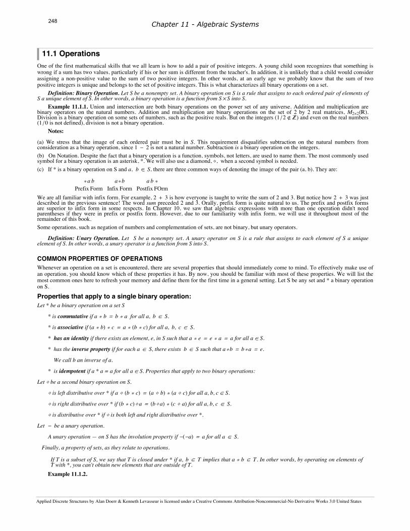
OPERATION TABLESIf the set on which an operation is defined is small, a table is often a good way of describing the operation. For example, we might want todefine Å⊕ on 80, 1, 2< by

a Å⊕b = : a + b if a + b < 3a + b - 3 if a + b ¥ 3

The table for Å⊕ is

"

Å⊕ 0 1 2

0 0 1 2

1 1 2 0

2 2 0 1

The top row and left column are the column and row headings, respectively. To determine aÅ⊕b, find the entry in Row a and Column b. Thefollowing operation table serves to define * on 8i, j, k<.

"

* i j k

i i i i

j j j j

k k k k

Note that; j*k = j, yet k * j = k. Thus, * is not commutative. Commutivity is easy to identify in a table: the table must be symmetric withrespect to the diagonal going from the top left to lower right.

EXERCISES FOR SECTION 11.1A Exercises1. Determine the properties that the following operations have on the positive integers.

(a) addition

(b) multiplication

(c) M defined by a M b = larger of a and b

(d) m defined by a m b = smaller of a and b

(e) @ defined by a ü b = ab

2. Which pairs of operations in Exercise 1 are distributive over one another?

3. Let * be an operation on a set S and A, B Œ S. Prove that if A and B are both closed under *, then A › B is also closed under *, but A ‹ Bneed not be.4. How can you pick out the identity of an operation from its table?

5. Define a * b by a - b , the absolute value of a - b. Which properties does * have on the set of natural numbers, N?



249

11.2 Algebraic SystemsAn algebraic system is a mathematical system consisting of a set called the domain and one or more operations on the domain. If V is thedomain and *1 , *2 , …, *n are the operations, @V;*1, *2 , …, *nD denotes the mathematical system. If the context is clear, this notation isabbreviated to V.

Example 11.2.1.

(a) Let B* be the set of all finite strings of 0's and 1's including the null (or empty) string, l. An algebraic system is obtained by adding theoperation of concatenation. The concatenation of two strings is simply the linking of the two strings together in the order indicated. Theconcatenation of strings a with b is denoted a <> b. For example, "01101" <> "101" = "01101101" and l <> "100" = "100". Note thatconcatenation is an associative operation and that l is the identity for concatenation.

Note on Notation: There isn't a standard symbol for concatenation. We have chosen <> to be consistant with the notation used inMathematica for the StringJoin function, which does concatenation. Many programming languages use the plus sign for concatenation,but others use & or ||.(b) Let M be any nonempty set and let * be any operation on M that is associative and has in identity in M. Our second example might seemstrange, but we include it to illustrate a point. The algebraic system @B*; <>D is a special case of @M ;*D. Most of us are much more comfort-able with B* than with M. No doubt, the reason is that the elements in B* are more concrete. We know what they look like and exactly howthey are combined. The description of M is so vague that we don't even know what the elements are, much less how they are combined. Whywould anyone want to study M? The reason is related to this question: What theorems are of interest in an algebraic system? Answering thisquestion is one of our main objectives in this chapter. Certain properties of algebraic systems are called algebraic properties, and anytheorem that says something about the algebraic properties of a system would be of interest. The ability to identify what is algebraic and whatisn't is one of the skills that you should learn from this chapter.Now, back to the question of why we study M. Our answer is to illustrate the usefulness of M with a theorem about M.

Theorem 11.2.1. If a, b are elements of M and a * b = b * a, then Ha * bL * Ha * bL = Ha * aL * Hb * bL.Proof:

Ha*bL* Ha*bL = a* Hb* Ha*bLL= a* HHb*aL*bL= a* HHa*bL*bL= a* Ha* Hb*bLL= Ha*aL* Hb*bL

Why?Why?Why?Why?Why?

The power of this theorem is that it can be applied to any algebraic system that M describes. Since B* is one such system, we can applyTheorem 11.2.1 to any two strings that commute—for example, 01 and 0101. Although a special case of this theorem could have been provenfor B*, it would not have been any easier to prove, and it would not have given us any insight into other special cases of M .Example 11.2.2. Consider the set of 2µ2 real matrices, M2µ2HRL, with the operation of matrix multiplication. In this context, Theorem 11.2.1

can be interpreted as saying that if A B = B A, then HA BL2 = A2 B2. One pair of matrices that this theorem applies to is K 2 11 2 O and

K 3 -4-4 3 O.

LEVELS OF ABSTRACTIONOne of the fundamental tools in mathematics is abstraction. There are three levels of abstraction that we will identify for algebraic systems:concrete, axiomatic, and universal.Concrete Level. Almost all of the mathematics that you have done in the past was at the concrete level. As a rule, if you can give examples of afew typical elements of the domain and describe how the operations act on them, you are describing a concrete algebraic system. Two examplesof concrete systems are B* and M2µ2HRL. A few others are:(a) The integers with addition. Of course, addition isn't the only standard operation that we could include. Technically, if we were to addmultiplication, we would have a different system.(b) The subsets of the natural numbers, with union, intersection, and complementation.

(c) The complex numbers with addition and multiplication.

Axiomatic Level. The next level of abstraction is the axiomatic level. At this level, the elements of the domain are not specified, but certainaxioms are stated about the number of operations and their properties. The system that we called M is an axiomatic system. Some combinationsof axioms are so common that a name is given to any algebraic system to which they apply. Any system with the properties of M is called amonoid. The study of M would be called monoid theory. The assumptions that we made about M, associativity and the existence of an identity,are called the monoid axioms. One of your few brushes with the axiomatic level may have been in your elementary algebra course. Manyalgebra texts identify the properties of the real numbers with addition and multiplication as the field axioms. As we will see in Chapter 16,"Rings and Fields," the real numbers share these axioms with other concrete systems, all of which are called fields.Universal Level. The final level of abstraction is the universal level. There are certain concepts, called universal algebra concepts, that can beapplied to the study of all algebraic systems. Although a purely universal approach to algebra would be much too abstract for our purposes,defining concepts at this level should make it easier to organize the various algebraic theories in your own mind. In this chapter, we willconsider the concepts of isomorphism, subsystem, and direct product.



250

GROUPSTo illustrate the axiomatic level and the universal concepts, we will consider yet another kind of axiomatic system, the group. In Chapter 5 wenoted that the simplest equation in matrix algebra that we are often called upon to solve is A X = B, where A and B are known square matricesand X is an unknown matrix. To solve this equation, we need the associative, identity, and inverse laws. We call the systems that have theseproperties groups.

Definition: Group. A group consists of a nonempty set G and an operation * on G satisfying the properties

(a) * is associative on G: Ha*bL*c = a* Hb*cL for all a, b, c œ G.

(b) There exists an identity element, e œ G such that a*e = e*a = a for all a œ G.

(c) For all a œ G, there exists an inverse, there exist b œ G such that a *b = b*a = e.

A group is usually denoted by its set's name, G, or occasionally by @G; * D to emphasize the operation. At the concrete level, most sets have astandard operation associated with them that will form a group. As we will see below, the integers with addition is a group. Therefore, in grouptheory Z always stands for @Z; +D.Generic Symbols. At the axiomatic and universal levels, there are often symbols that have a special meaning attached to them. In group theory,the letter e is used to denote the identity element of whatever group is being discussed. A little later, we will prove that the inverse of a groupelement, a, is unique and it is inverse is usually denoted a-1 and is read "a inverse." When a concrete group is discussed, these symbols aredropped in favor of concrete symbols. These concrete symbols may or may not be similar to the generic symbols. For example, the identityelement of the group of integers is 0, and the inverse of n is denoted by -n, the additive inverse of n.The asterisk could also be considered a generic symbol since it is used to denote operations on the axiomatic level.

Example 11.2.3.

(a) The integers with addition is a group. We know that addition is associative. Zero is the identity for addition: 0 + n = n + 0 = n for allintegers n. The additive inverse of any integer is obtained by negating it. Thus the inverse of n is -n.(b) The integers with multiplication is not a group. Although multiplication is associative and 1 is the identity for multiplication, not allintegers have a multiplicative inverse in Z. For example, the multiplicative inverse of 10 is 1

10, but 1

10 is not an integer.

(c) The power set of any set U with the operation of symmetric difference, Å⊕, is a group. If A and B are sets, thenAÅ⊕B = HA ‹ BL - HA › BL. We will leave it to the reader to prove that Å⊕ is associative over PHUL. The identity of the group is the empty set:AÅ⊕ « = A. Every set is its own inverse since A Å⊕ A = «. Note that PHUL is not a group with union or intersection.

Definition: Abelian Group. A group is abelian if its operation is commutative.

Most of the groups that we will discuss in this book will be abelian. The term abelian is used to honor the Norwegian mathematician N. Abel(1802-29), who helped develop group theory.

Norwegian Stamp honoring Abel

EXERCISES FOR SECTION 11.2A Exercises1. Discuss the analogy between the terms generic and concrete for algebraic systems and the terms generic and trade for prescription drugs.

2. Discuss the connection between groups and monoids. Is every monoid a group? Is every group a monoid?

3. Which of the following are groups?



251

(a) B* with concatenation (Example 11.2.1a).

(b) M2µ3HRL with matrix addition.

(c) M2µ3HRL with matrix multiplication.

(d) The positive real numbers, R+, with multiplication.

(e) The nonzero real numbers, R*, with multiplication.

(f) 81, -1< with multiplication.

(g) The positive integers with the operation M defined by a M b = larger of a and b.

4. Prove that, Å⊕, defined by A Å⊕ B = HA ‹ BL - HA › BL is an associative operation on PHUL.5. The following problem supplies an example of a non-abelian group. A rook matrix is a matrix that has only 0's and 1's as entries such thateach row has exactly one 1 and each column has exactly one 1. The term rook matrix is derived from the fact that each rook matrix representsthe placement of n rooks on an nµn chessboard such that none of the rooks can attack one another. A rook in chess can move only vertically orhorizontally, but not diagonally. Let Rn be the set of nµn rook matrices. There are six 3µ3 rook matrices:

I =1 0 00 1 00 0 1

R1 =0 1 00 0 11 0 0

R2 =0 0 11 0 00 1 0

F1 =1 0 00 0 10 1 0

F2 =0 0 10 1 01 0 0

F3 =0 1 01 0 00 0 1

(a) List the 2µ2 rook matrices. They form a group, R2, under matrix multiplication. Write out the multiplication table. Is the group abelian?

(b) Write out the multiplication table for R3 . This is another group. Is it abelian?

(c) How many 4µ4 rook matrices are there? How many nµ n rook matrices are there?

6. For each of the following sets, identify the standard operation that results in a group. What is the identity of each group?

(a) The set of all 2µ2 matrices with real entries and nonzero determinants.

(b) The set of 2 µ 3 matrices with rational entries.

B Exercises7. Let V = 8e, a, b, c<. Let * be defined (partially) by x * x = e for all x œ V . Write a complete table for * so that @V; * D is a group.



252

11.3 Some General Properties of GroupsIn this section, we will present some of the most basic theorems of group theory. Keep in mind that each of these theorems tells us somethingabout every group. We will illustrate this point at the close of the section.

Theorem 11.3.1. The identity of a group is unique.

One difficulty that students often encounter is how to get started in proving a theorem like this. The difficulty is certainly not in the theorem'scomplexity. Before actually starting the proof, we rephrase the theorem so that the implication it states is clear.

Theorem 11.3.1 (Rephrased). If G = @G; *D is a group and e is an identity of G, then no other element of G is an identity of G.

Proof (Indirect): Suppose that f œ G, f ¹≠ e, and f is an identity of G. We will show that f = e, a contradiction, which completes theproof:

f = f * e Since e is an identity.

= e. Since f is an identity. ‡

Theorem 11.3.2. The inverse of any element of a group is unique.

The same problem is encountered here as in the previous theorem. We will leave it to the reader to rephrase this theorem. The proof is also leftto the reader to write out in detail. Here is a hint: If b and c are both inverses of a, then you can prove that b = c. lf you have difficulty withthis proof, note that we have already proven it in a concrete setting in Chapter 5.The significance of Theorem 11.3.2 is that we can refer to the inverse of an element without ambiguity. The notation for the inverse of a isusually a-1. (note the exception below).

Example 11.3.1.

(a) In any group, e-1 is the inverse of the identity e, which always is e.

(b) Ha-1L-1 is the inverse of a-1 , which is always equal to a (see Theorem 11.3.3 below).

(c) Hx* y* zL-1 is the inverse of x * y * z.(d) In a concrete group with an operation that is based on addition, the inverse of a is usually written -a. For example, the inverse of k - 3in the group @Z; +D is written -Hk - 3L = 3 - k. In the group of 2 µ 2 matrices over the real numbers under matrix addition, the inverse of

K 4 11 -3 O is written -K 4 1

1 -3 O, which equals K -4 -1-1 3 O.

Theorem 11.3.3. If a is an element of group G, then Ia-1M-1 = a.

Theorem 11.3.3 (Rephrased). If a has inverse b and b has inverse c, then a = c.

Proof:

a = a * Hb * cL because c is the inverse of b

= Ha * bL * c why?

= e * c why?

= c. by the identity property of e. ‡

Theorem 11.3.4. If a and b are elements of group G, then Ha*bL-1 = b-1 *a-1

Note: This theorem simply gives you a formula for the inverse of a * b. This formula should be familiar. In Chapter 5 we saw that if Aand B are invertible matrices, then HA BL-1 = B-1 A-1 .

Proof: Let x = b-1 *a-1. We will prove that x inverts a * b. Since we know that the inverse is unique, we will have prove the theorem.

Ha * bL * x = Ha * bL * Hb-1 *a-1L= a* Hb* Hb-1 *a-1LL= a* HHb*b-1L*a-1L= a * He * a-1L= a * a-1= e

Similarly, x * Ha * bL = e; therefore, Ha*bL-1 = x = b-1 *a-1 ‡Theorem 11.3.5. Cancellation Laws. If a, b, and c are elements of group G, both a * b = a * c and b * a = c * a imply that b = c.

Proof: Since a * b = a * c, we can operate on both a * b and a * c on the left with a-1 :



253

a-1 * Ha * bL = a-1 * Ha * cLApplying the associative property to both sides we get

Ha-1 * aL * b = Ha-1 * aL * cor

e * b = e * c

and finally

b = c.

This completes the proof of the left cancellation law. The right law can be proven in exactly the same way. ‡

Theorem 11.3.6. Linear Equations in a Group. If G is a group and a, b, œ G, the equation a * x = b has a unique solution,x = a-1 * b. In addition, the equation x * a = b has a unique solution, x = b * a-1 .

Proof: (for a * x = b):

a* x = b= e * b= Ha* a-1L * b= a * Ha-1 * bL

By the cancellation law, we can conclude that x = a -1 * b.

If c and d are two solutions of the equation a * x = b, then a * c = b = a * d and, by the cancellation law, c = d. This verifies that a -1 * bis the only solution of a * x = b. ‡

Note: Our proof of Theorem 11.3.6 was analogous to solving 4 x = 9 in the following way:

4 x = 9 = I4 ÿ 14M 9 = 4 I 1

49M

Therefore, by cancelling 4,

x = 14ÿ 9 = 9

4.

Exponentiation in a GroupIf a is an element of a group G, then we establish the notation that

a * a = a2

a*a*a = a3etc.

In addition, we allow negative exponent and define, for example, a-2 = Ha2L-1Although this should be clear, proving exponentiation properties requires a more precise recursive definition:

Definition: Exponentiation in a Group. For n ¥ 0, define an recursively by a 0 = e and if n > 0, an = an-1 *a. Also, if n > 1,a-n = HanL-1 .

Example 11.3.2.

(a) In the group of positive real numbers with multiplication,

53 = 52 ÿ5 = H51 ÿ5L ÿ5 = HH50 ÿ5L ÿ5L ÿ5 = HH1 ÿ5L ÿ5L ÿ5 = 5 ÿ5 ÿ5 = 125.and

5-3 = H125L-1 = 1125

(b) In a group with addition, we use a different form of notation, reflecting the fact that in addition repeated terms are multiples, not powers.For example, in @Z; +D, a + a is written as 2 a, a + a + a is written as 3 a, etc. The inverse of a multiple of a such as- Ha + a + a + a + aL = -H5 aL is written as H-5L a.

Although we define, for example, a5 = a4 * a, we need to be able to extract the single factor on the left. The following lemma justifies doingprecisely that.

Lemma. Let G be a group. If b œ G and n ¥ 0, then bn+1 = b* bn, and hence b* bn = bn *b. Proof (by induction): If n = 0,



254

b1 = b0 *b by the definition of exponentiation= e*b basis for exponentiation= b * e identity property= b * b0 basis for exponentiation

Now assume the formula of the lemma is true for some n ¥ 0,

bHn+1L+1 = bHn+1L * b by the definition of exponentiation= Hb*bnL*b by the induction hypothesis= b* Hbn *bL associativity= b* Hbn+1L definition of exponentiation ‡

Based on the definitions for exponentiation above, there are several properties that can be proven. They are all identical to the exponentiationproperties from elementary algebra.

Theorem 11.3.7. Properties of Exponentiation. If a is an element of a group G, and n and m are integers,

(a) a-n = Ia-1Mn and hence HanL-1 = Ia-1Mn(b) an+m = an *am

(c) HanLm = an m

We will leave the proofs of these properties to the interested reader. All three parts can be done by induction. For example the proof of (b)would start by defining the proposition pHmL , m ¥ 0, to be an+m = an *am for all n . The basis is pH0L : an+0 = an *a0.Our final theorem is the only one that contains a hypothesis about the group in question. The theorem only applies to finite groups.

Theorem 11.3.8. If G is a finite group, †G§ = n, and a is an element of G, then there exists a positive integer m such that am = e andm § n.

Proof: Consider the list a, a2, …, an+1 . Since there are n + 1 elements of G in this list, there must be some duplication. Suppose thatap = aq, with p < q. Let m = q - p. Then

am = aq-p = aq *a-p = aq * HapL-1 = aq * HaqL-1 = eFurthermore, since 1 § p < q § n + 1, m = q - p § n. ‡

Consider the concrete group [Z; +]. All of the theorems that we have stated in this section except for the last one say something about Z.Among the facts that we conclude from the theorems about Z are:

Since the inverse of 5 is -5, the inverse of -5 is 5.

The inverse of -6 + 71 is -H71L + -H-6L = -71 + 6.

The solution of 12 + x = 22 is x = -12 + 22.

-4 H6L + 2 H6L = H-4 + 2L H6L = -2 H6L = -H2L H6LL.7 H4 H3LL = H7 ÿ4L H3L = 28 H3L (twenty-eight 3s).

EXERCISES FOR SECTION 11.3A Exercises1. Let @G; * D be a group and a be an element of G. Define f : G Ø G by f HxL = a * x.

(a) Prove that f is a bijection.

(b) On the basis of part a, describe a set of bijections on the set of integers.

2. Rephrase Theorem 11.3.2 and write out a clear proof.

3. Prove by induction on n that if a1, a2, …, an are elements of a group G, n ¥ 2, then

Ha1 *a2 *º⋯*anL-1 = an-1 *º⋯*a2-1 *a1-1. Interpret this result in terms of [Z; +] and @R;*D.4. True or false? If a, b, c are elements of a group G, and a * b = c * a, then b = c. Explain your answer.

5. Prove Theorem 11.3.7.

6. Each of the following facts can be derived by identifying a certain group and then applying one of the theorems of this section to it. Foreach fact, list the group and the theorem that are used.



255

(a) I 13M 5 is the only solution of 3 x = 5.

(b) -H-H-18LL = -18.

(c) If A, B, C are 3µ3 matrices over the real numbers, with A + B = A + C, then B = C.

(d) There is only one subset of the natural numbers for which K Å⊕ A = A for every A Œ N.



256

11.4 Zn, the Integers Modulo nIn this section we introduce a collection of concrete groups, one for each positive integer, that will provide us with a wealth of examples andapplications. We start with a theorem about integer division that is intuitively clear. We leave the proof as an optional exercise.

The Division Property for Integers. If m, n œ Z , n > 0, then there exist two unique integers, q (quotient) and r (remainder), such thatm = n q + r and 0 § r < n.

Note: The division property says that if m is divided by n, you will obtain a quotient and a remainder, where the remainder is less than n.This is a fact that most elementary school students learn when they are introduced to long division. In doing the division problem 1986 ¸ 97,you obtain a quotient of 20 and a remainder of 46. This result could either be written 1986

97= 20 + 46

97 or 1986 = 97 ÿ20 + 46. The later

form is how the division property is normally expressed.If two numbers, a and b, share the same remainder after dividing by n. we say that they are congruent modulo n, denoted a ª b Hmod nL. Forexample, 13 ª 38 Hmod 5L because 13 = 5 ÿ2 + 3 and 38= 5· + 3.

Modular Arithmetic. If n is a positive integer, we define the operations of addition modulo n H+n) and multiplication modulo n Hµn) asfollows. If a, b œ Z ,

a +n b = the remainder after a + b is divided by n

a µn b = the remainder after a ÿ b is divided by n.

Notes:

(a) The result of doing arithmetic modulo n is always an integer between 0 and n - 1, by the Division Property. This observation implies that80, 1, ..., n - 1< is closed under modulo n arithmetic.(b) It is always true that a +n b ª Ha + bL Hmod nL and aµn b ª Ha ÿ bL Hmod nL. For example, 4 +7 5 = 2 ª 9 Hmod 7L and

4 µ7 5 ª 6 ª 20 Hmod 7L.(c) We will use the notation Zn to denote the set 80, 1, 2, . . ., n - 1<.Properties of Modular Arithmetic on ZnAddition modulo n is always commutative and associative; 0 is the identity for +n and every element of Zn has an additive inverse.

Multiplication modulo n is always commutative and associative, and 1 is the identity for µn.

Theorem 11.4.1. If a œ Zn, a ¹≠ 0, then the additive inverse of a is n - a.

Proof: a + Hn - aL = n ª 0 Hmod nL , since n = n ÿ1 + 0. Therefore, a +n Hn - aL = 0 ‡

Note: The algebraic properties of +n and µn on Zn are identical to the properties of addition and multiplication on Z.

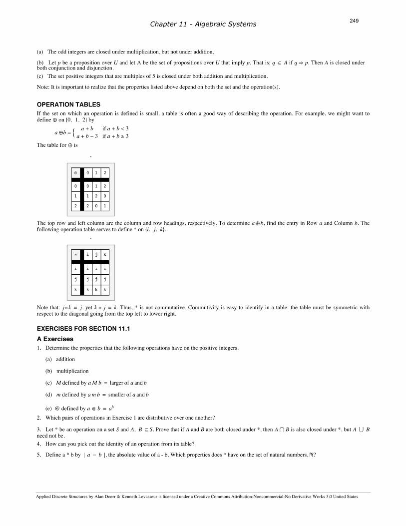
The Group Zn. For each n ¥ 1, @Zn; +nD is a group. Henceforth, we will use the abbreviated notation Zn when referring to this group. Figure11.4.1 contains the tables for Z1 through Z6.

Figure 11.4.1Addition tables for Zn, 1£n£6.

Example 11.4.1.

(a) We are all somewhat familiar with Z12 since the hours of the day are counted using this group, except for the fact that 12 is used in placeof 0. Military time uses the mod 24 system and does begin at 0. If someone started a four-hour trip at hour 21, the time at which she wouldarrive is 21 +24 4 = 1. If a satellite orbits the earth every four hours and starts its first orbit at hour 5, it would end its first orbit at time5 4 9 I h bi ld d 5 7 4 9 h h l k



257

y , 5 +24 4 = 9. Its tenth orbit would end at 5 +24 7µ24 4 = 9 hours on the clock(b) Virtually all computers represent unsigned integers in binary form with a fixed number of digits. A very small computer might reserveseven bits to store the value of an integer. There are only 27 different values that can be stored in seven bits. Since the smallest value is 0,represented as 0000000, the maximum value will be 27 - 1 = 127, represented as 1111111. When a command is given to add two integervalues, and the two values have a sum of 128 or more, overflow occurs. For example, if we try to add 56 and 95, the sum is an eight-digitbinary integer 10010111. One common procedure is to retain the seven lowest-ordered digits. The result of adding 56 and 95 would be0 010 111two = 23 ª 56 + 95 Hmod 128L. Integer arithmetic with this computer would actually be modulo 128 arithmetic.

Mathematica Note

Most computer languages have a "mod" function that computes the remainder when one integer is divided by another. Mathematica is noexception. To determine the remainder upon dividing 1986 by 97 we can evaluate

Mod@1986, 97D46

A mod 6 addition function can be defined based on Mod with the following input:

Plus6@a_, b_D := Mod@a + b, 6DThere is a free package called AbstractAlgebra that is available at http://www.central.edu/eaam/index.asp. It contains a function that willgenerate the operation tables, also called Cayley Tables, such you see in Figure 11.4.1. First load the package, as instructed:

<< AbstractAlgebra`Master`

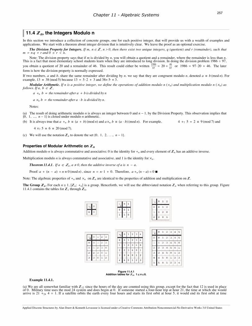
We can form a the group Z6 using the FormGroupoid function:

G = FormGroupoid@Range@0, 5D, Plus6DGroupoidH80, 1, 2, 3, 4, 5<, -Operation-L

Then the function called CayleyTable generates the table for the group Z6:

CayleyTable@G, BodyColored Ø False,HeadingsColored Ø False, ShowExtraCayleyInformation Ø FalseD

TheGroupy

x

* 0 1 2 3 4 5

0 0 1 2 3 4 5

1 1 2 3 4 5 0

2 2 3 4 5 0 1

3 3 4 5 0 1 2

4 4 5 0 1 2 3

5 5 0 1 2 3 4

Note: The rules BodyColored Æ False, HeadingsColored Æ False, ShowExtraCayleyInformation Æ False are included in the inputabove for easier print readability. They would not be normally included when using CayleyTable. It's actually even easier to generate these tables because the family of Zn ' s is part of the package. Here is the table for Z9:



258

CayleyTable@Z@9D, BodyColored Ø False,HeadingsColored Ø False, ShowExtraCayleyInformation Ø FalseD

Z@9Dy

x

+ 0 1 2 3 4 5 6 7 8

0 0 1 2 3 4 5 6 7 8

1 1 2 3 4 5 6 7 8 0

2 2 3 4 5 6 7 8 0 1

3 3 4 5 6 7 8 0 1 2

4 4 5 6 7 8 0 1 2 3

5 5 6 7 8 0 1 2 3 4

6 6 7 8 0 1 2 3 4 5

7 7 8 0 1 2 3 4 5 6

8 8 0 1 2 3 4 5 6 7

Sage Note

Sage has some extremely powerful tool for working with groups, although the operation tables of groups Zn are not all that easy to create.Here is a very simple calculation with mod 6 arithmetic.

R = IntegerModRing(6)a = R(3) + R(5)*R(2)a 1

There is a built in family of groups that is essentially the same as the Zn ' s. Here is the one that corresponds with Z6, where the letters athrough f would be replaced with 0 through 5.

G=CyclicPermutationGroup(6)G.cayley_table()

* a b c d e f+------------a a b c d e fb b c d e f ac c d e f a bd d e f a b ce e f a b c df f a b c d e

EXERCISES FOR SECTION 11.4A Exercises1. Calculate:

(a) 7 +8 3

(b) 7 µ8 3

(c) 4µ8 4

(d) 10 +12 2

(e) 6µ8 2 +8 6µ8 5

(f) 6µ8 H2 +8 5L(g) 3 µ5 3 µ5 3 µ5 3 ª 34 Hmod 5L (h) 2 µ11 7



259

(i) 2 µ14 7

2. List the additive inverses of the following elements:

(a) 4, 6, 9 in Z10

(b) 16, 25, 40 in Z503. In the group Z11 , what are:

(a) 3(4)?

(b) 36(4)?

(c) How could you efficiently compute m H4L, m œ Z?

4. Prove that {1, 2, 3, 4} is a group under the operation µ5.

5. A student is asked to solve the following equations under the requirement that all arithmetic should be done in Z2. List all solutions.

(a) x2 + 1 = 0.

(b) x2 + x + 1 = 0.6. Determine the solutions of the same equations as in Exercise 5 in Z5.

B Exercises7. Prove the division property by induction on m.

8. Prove that congruence modulo n is an equivalence relation on the integers. Describe the set of equivalence classes that congruence modulon defines.



260

11.5 SubsystemsThe subsystem is a fundamental concept of algebra at the universal level.

Definition: Subsystem. If @V; *1, …, *nD is an algebraic system of a certain kind and W is a subset of V, then W is a subsystem of V if@W; *1, …, *nD is an algebraic system of the same kind as V. The usual notation for "W is a subsystem of V" is W § V.Since the definition of a subsystem is at the universal level, we can cite examples of the concept of subsystems at both the axiomatic andconcrete level.

Example 11.5.1

(a) (Axiomatic) If @G; *D is a group, and H is a subset of G, then H is a subgroup of G if @H; *D is a group.

(b) (Concrete) U = 8-1, 1< is a subgroup of @R*; ÿD. Take the time now to write out the multiplication table of U and convince yourself that@U; ÿD is a group.(c) (Concrete) The even integers, 2 Z = 82 k : k is an integer< is a subgroup of @Z; +D. Convince yourself of this fact.

(d) (Concrete) The set of nonnegative integers is not a subgroup of @Z; +D. All of the group axioms are true for this subset except one: nopositive integer has a positive additive inverse. Therefore, the inverse property is not true. Note that every group axiom must be true for asubset to be a subgroup.(e) (Axiomatic) If M is a monoid and P is a subset of M, then P is a submonoid of M if P is a monoid.

(f) (Concrete) If B* is the set of strings of 0's and 1's of length zero or more with the operation of concatenation, then two examples ofsubmonoids of B* are: (i) the set of strings of even length, and (ii) the set of strings that contain no 0's. The set of strings of length less than 50is not a submonoid because it isn't closed under concatenation. Why isn't the set of strings of length 50 or more a submonoid of B*?For the remainder of this section, we will concentrate on the properties of subgroups. The first order of business is to establish a systematic wayof determining whether a subset of a group is a subgroup.

Theorem/Algorithm 11.5.1. To determine whether H, a subset of group @G;*D, is a subgroup, it is sufficient to prove:

(a) H is closed under *; that is, a, b œ H a * b œ H;

(b) H contains the identity element for *; and

(c) H contains the inverse of each of its elements; that is, a œ H a-1 œ H.Proof: Our proof consists of verifying that if the three properties above are true, then all the axioms of a group are true for @H ; *D. By Condi-tion (a), * can be considered an operation on H. The associative, identity, and inverse properties are the axioms that are needed. The identityand inverse properties are true by Conditions (b) and (c), respectively, leaving only the associative property. Since, @G; *D is a group,a * Hb * cL = Ha * bL * c for all a, b, c œ G. Certainly, if this equation is true for all choices of three elements from G, it will be true for allchoices of three elements from H, since H is a subset of G. ‡For every group with at least two elements, there are at least two subgroups: they are the whole group and 8e<. Since these two are automatic,they are not considered very interesting and are called the improper subgroups of the group; 8e< is sometimes referred to as the trivial subgroup.All other subgroups, if there are any, are called proper subgroups.We can apply Theorem 11.5.1 at both the concrete and axiomatic levels.

Examples 11.5.2.

(a) (Concrete) We can verify that 2 Z § Z, as stated in Example 11.5.1. Whenever you want to discuss a subset, you must find someconvenient way of describing its elements. An element of 2 Z can be described as 2 times an integer; that is, a œ 2 Z is equivalent toH$ kLZ Ha = 2 kL. Now we can verify that the three conditions of Theorem 11.5.1 are true for 2Z. First, if a, b œ 2 Z, then there existj, k œ Z such that a = 2 j and b = 2 k. A common error is to write something like a = 2 j and b = 2 j. This would mean that a = b,which is not necessarily true. That is why two different variables are needed to describe a and b. Returning to our proof, we can add a andb:

a + b = 2 j + 2 k = 2 H j + kL. Since j + k is an integer, a + b is an element of 2 Z. Second, the identity, 0, belongs to 2Z (0 = 2 H0L). Finally, if a œ 2 Z anda = 2 k, -a = -H2 kL = 2 H-kL, and -k œ Z, therefore, -a œ 2 Z. By Theorem 11.5.1, 2 Z § Z.How would this argument change if you were asked to prove that 3 Z § Z? or n Z § Z, n ¥ 2?

(b) (Concrete) We can prove that H = 80, 3, 6, 9< is a subgroup of Z12 . First, for each ordered pair Ha, bL œ H µ H, a +12 b is in H.This can be checked without too much trouble since †H µH§ = 16. Thus we can conclude that H is closed under +12. Second, 0 œ H. Third,-0 = 0, -3 = 9, -6 = 6, and -9 = 3. Therefore, the inverse of each element in H is in H.(c) (Axiomatic) If H and K are both subgroups of a group G, then H › K is a subgroup of G. To justify this statement, we have no concreteinformation to work with, only the facts that H § G and K §G. Our proof that H › K § G reflects this and is an exercise in applying thedefinitions of intersection and subgroup, (i) If a and b are elements of H › K, then a and b both belong to H, and since H § G, a * b must bean element of H. Similarly, a * b œ K; therefore, a * b œ H › K. (ii) The identity of G must belong to both H and K; hence it belongs toH › K. (iii) If a œ H › K, then a œ H, and since H § G, a-1 œ H. Similarly, a-1 œ K. Hence, by the theorem, H › K § G.Now that this fact has been established, we can apply it to any pair of subgroups of any group. For example, since 2 Z and 3 Z are bothsubgroups of @Z; +D, 2 Z › 3 Z is also a subgroup of Z. Note that if a œ 2 Z › 3 Z, a must have a factor of 3; that is, there exists k œ Z

h h 3 k I ddi i b h f k b Th i j Z h h k 2 j h f 3 H2 jL 6 j


261

such that a = 3 k. In addition, a must be even, therefore k must be even. There exists j œ Z such that k = 2 j, therefore a = 3 H2 jL = 6 j.This shows that 2 Z› 3 Z Œ 6 Z. The opposite containment can easily be established; therefore, 2 Z › 3 Z = 6 Z.Given a finite group, we can apply Theorem 11.3.7 to obtain a simpler condition for a subset to be a subgroup.

Theorem/Algorithm 11.5.2. If @G; * D is a finite group, H is a nonempty subset of G, and you can verify that H is closed under * , then His a subgroup of G.

Proof: In this proof, we demonstrate that Conditions (b) and (c) of Theorem 11.5.1 follow from the closure of H under * , which isCondition (a). First, select any element of H; call it b. The powers of b : b1, b2, b3, … are all in H by the closure property. By Theorem11.3.7, there exists m, m § †G§, such that bm = e; hence e œ H. To prove that (c) is true, we let a be any element of H. If a = e, then a-1 is inH since e-1 = e. If a ¹≠ e, aq = e for some q between 2 and †G§ and

e = aq = a q-1 * a.

Therefore, a-1 = aq-1 , which belongs to H since q - 1 ¥ 1. ‡Example 11.5.3 To determine whether H1 = 80, 5, 10< and H2 = 80, 4, 8, 12< are subgroups of Z15 , we need only write out the additiontables (modulo 15) for these sets.

H1 H2

y

x

+ 0 5 10

0 0 5 10

5 5 10 0

10 10 0 5

y

x

* 0 4 8 12

0 0 4 8 12

4 4 8 12 1

8 8 12 1 5

12 12 1 5 9

Note that H1 is a subgroup of Z15. Since the interior of the addition table for H2 contains elements that are outside of H2 , H2 is not a subgroupof Z15.One kind of subgroup that merits special mention due to its simplicity is the cyclic subgroup.

Definition: Cyclic Subgroup Generated by an Element. If G is a group and a œ G, the cyclic subgroup generated by a, HaL, is the set ofpowers of a and their inverses:

HaL = 8an : n œ Z <A subgroup H is cyclic if there exists a œ H such that H = HaL.

Definition: Cyclic Group. A group G is cyclic if there exists b œ G such that Hb L = G.

Note: If the operation on G is additive, then HaL = 8HnL a : n œ Z<. Example 11.5.4.

(a) In @R ; ÿD, H2L = 82n : n œ Z< = 9…, 116

, 18

, 1412

, 1, 2, 4, 8, 16, …=.(b) In Z15, H6L = 80, 3, 6, 9, 12}. If G is finite, you need list only the positive powers of a up to the first occurrence of the identity toobtain all of (a). In Z15 , the multiples of 6 are 6, H2L 6 = 12, H3L 6 = 3, H4L 6 = 9, and H5L 6 = 0. Note that 80, 3, 6, 9, 12< is also H3L, H9L,and H12L. This shows that a cyclic subgroup can have different generators.If you want to list the cyclic subgroups of a group, the following theorem can save you some time.

Theorem 11.5.3. If a is an element of group G, then HaL = Ha-1L. This is an easy way of seeing that H9L in Z15 equals H6L, since -6 = 9.

EXERCISES FOR SECTION 11.5A Exercises1. Which of the following subsets of the real numbers is a subgroup of @R; +D?

(a) the rational numbers

(b) the positive real numbers

(c) 8k ê2 k is an integer<(d) 92k k is an integer=



262

(e) 8x -100 § x § 100<2. Describe in simpler terms the following subgroups of Z:

(a) 5 Z › 4 Z

(b) 4 Z › 6 Z (be careful)

(c) the only finite subgroup of Z

3. Find at least two proper subgroups of R3 , the set of 3µ3 rook matrices (see Exercise 5 of Section 11.2).

4. Where should you place the following in Figure 11.5.1?

(a) e

(b) a-1

(c) x * y

GH K

a

x

y

Figure 11.5.1

5. (a) List the cyclic subgroups of Z6 and draw an ordering diagram for

the relation "is a subset of" on these subgroups.

(b) Do the same for Z12 .

(c) Do the same for Z8 .

(d) On the basis of your results in parts a, b, and c, what would you expect if you did the same with Z24?

B Exercises6. Subgroups generated by subsets of a group. The concept of a cyclic subgroup is a special case of the concept that we will discuss here. Let@G; * D be a group and S a nonempty subset of G. Define the set HSL recursively by:

(i) If a œ S, then a œ HSL,(ii) If a, b œ HSL, then a * b œ HSL, and

(iii) If a œ HSL, then a-1 œ HSL.(a) By its definition, HSL has all of the properties needed to be a subgroup of G. The only thing that isn't obvious is that the identity of G is in(S). Prove that the identity of G is in HSL. (b) What is H89, 15<L in @Z; +D?(c) Prove that if H § G and S Œ H, then HSL § H. This proves that HSL is contained in every subgroup of G that contains S; that is, HSL = ›

SŒHH§G

H .

(d) Describe H80.5, 3<L in @R+; ÿD and in [R; +] .

(e) If j, k œ Z, H8 j, k<L is a cyclic subgroup of Z. In terms of j and k, what is a generator of H8 j, k<L?7. Prove that if H, K § G, and H ‹ K = G, then H = G or K = G. (Hint: Use an indirect argument.)



263

11.6 Direct Products

Our second universal algebraic concept lets us look in the opposite direction from subsystems. Direct products allow us to create larger systems.In the following definition, we avoid complicating the notation by not specifying how many operations the systems have.

Definition: Direct Product. If @V1;*1, ù1 , …D, @V2;*2, ù2 , …D, …, @V1;*n, ùn , …D are algebraic systems of the same kind, then thedirect product of these systems is V = V1µV2µº⋯µVn , with operations defined below. The elements of V are n-tuples of the formHa1, a2, . . . , a n L, where ak œ Vk, k = 1, . . . , n. The systems V1, V2, …, Vn are called the factors of V. There are as many operations on Vas there are on the factors. Each of these operations is defined componentwise:If Ha1, a2, . . . , a n L, Hb1, b2, . . . , b n L œ V,

Ha1, a2, . . . , a n L* Hb1, b2, . . . , b n L = Ha1 *1 b1, a2 *2 b2, …, an *n bnLHa1, a2, . . . , a n Lù Hb1, b2, . . . , b n L = Ha1 ù1 b1, a2 ù2 b2, …, an ùn bnLª

Example 11.6.1. Consider the monoids N (the set of natural numbers with addition) and B* (the set of finite strings of 0's and 1's withconcatenation). The direct product of N with B* is a monoid. We illustrate its operation, which we will denote by * , with examples:H4, 001L * H3, 11L = H4 + 3, 001 <> 11L = H7, 00 111L

H0, 11 010L * H3, 01L = H3, 1 101 001LH0, lL * H129, 00 011L = H0 + 129, l <> 00 011L = H129, 00 011LH2, 01L * H8, 10L = H10, 0110L, and

H8, 10L * H2, 01L = H10, 1001L.Note that our new monoid is not commutative. What is the identity for * ?

Notes:

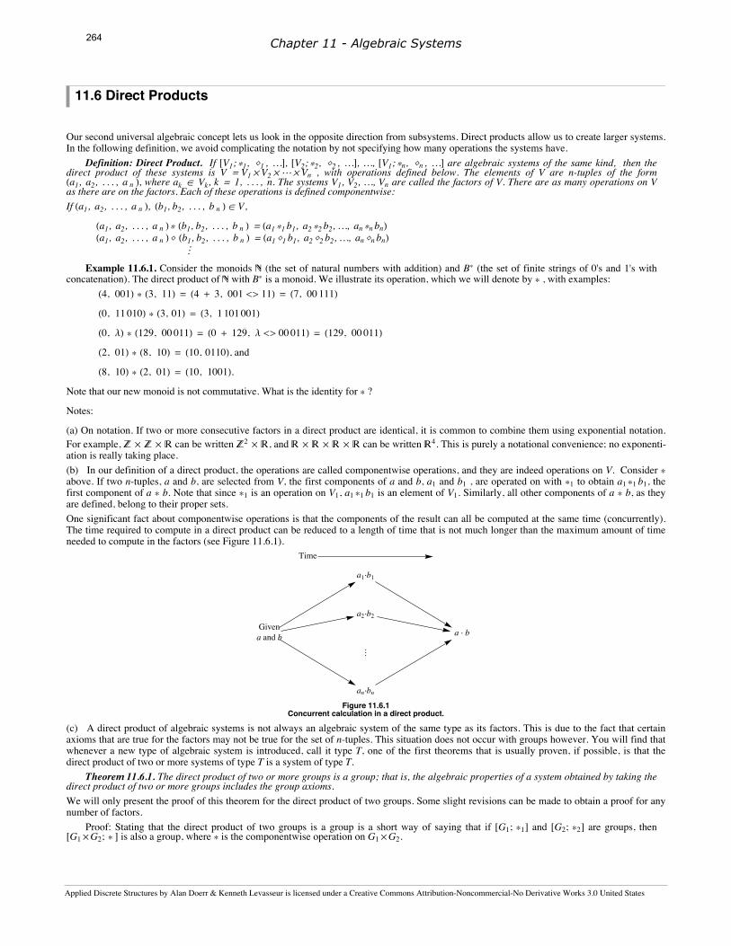
(a) On notation. If two or more consecutive factors in a direct product are identical, it is common to combine them using exponential notation.For example, Z µ Z µ R can be written Z2 µ R, and R µ R µ R µ R can be written R4. This is purely a notational convenience; no exponenti-ation is really taking place.(b) In our definition of a direct product, the operations are called componentwise operations, and they are indeed operations on V. Consider *above. If two n-tuples, a and b, are selected from V, the first components of a and b, a1 and b1 , are operated on with *1 to obtain a1 *1 b1, thefirst component of a * b. Note that since *1 is an operation on V1, a1 *1 b1 is an element of V1. Similarly, all other components of a * b, as theyare defined, belong to their proper sets.One significant fact about componentwise operations is that the components of the result can all be computed at the same time (concurrently).The time required to compute in a direct product can be reduced to a length of time that is not much longer than the maximum amount of timeneeded to compute in the factors (see Figure 11.6.1).

Givena and b a ÿ b

a1ÿb1

a2ÿb2

ª

anÿbn

Time

Figure 11.6.1Concurrent calculation in a direct product.

(c) A direct product of algebraic systems is not always an algebraic system of the same type as its factors. This is due to the fact that certainaxioms that are true for the factors may not be true for the set of n-tuples. This situation does not occur with groups however. You will find thatwhenever a new type of algebraic system is introduced, call it type T, one of the first theorems that is usually proven, if possible, is that thedirect product of two or more systems of type T is a system of type T.

Theorem 11.6.1. The direct product of two or more groups is a group; that is, the algebraic properties of a system obtained by taking thedirect product of two or more groups includes the group axioms.We will only present the proof of this theorem for the direct product of two groups. Some slight revisions can be made to obtain a proof for anynumber of factors.

Proof: Stating that the direct product of two groups is a group is a short way of saying that if @G1; *1D and @G2; *2D are groups, then@G1µG2; * D is also a group, where * is the componentwise operation on G1µG2.



264

Associativity of * : If a, b, c œ G1µG2,

a * Hb * cL = Ha1, a2L* HHb1, b2L* Hc1, c2LL= Ha1, a2L* Hb1 *1 c1, b2 *2 c2L= Ha1 *1 Hb1 *1 c1L, a2 *2 Hb2 *2 c2LL= HHa1 *1 b1L*1 c1, Ha2 *2 b2L*2 c2L= Ha1 *1 b1, a2 *2 b2L* Hc1, c2L= HHa1, a2L* Hb1, b2LL* Hc1, c2L= Ha * bL*c

Notice how the associativity property hinges on the associativity in each factor.

An identity for *: As you might expect, if e1 and e2 are identities for G1 and G2, respectively, then e = He1, e 2 L is the identity for G1µG2. Ifa œ G1µG2,

a * e = Ha1, a2L* He1, e 2 L= Ha1 *1 e1, a2 *2 e 2L= Ha1, a2L= a

Similarly, e * a = a.

Inverses in G1µG2: The inverse of an element is determined componentwise a-1 = Ha1, a2L-1 = Ha1-1, a2-1L . To verify, we compute a * a-1 :

a * a-1 = Ha1, a2L* Ha1-1, a2-1L= Ha1 *1 a1-1, a2 *2 a2-1L= He1, e 2 L= e

Similarly, a-1 * a = e. ‡Example 11.6.2.

(a) If n ¥ 2, Z2n , the direct product of n factors of Z2, is a group with 2n elements. We will take a closer look at Z23 = Z2 µ Z2 µ Z2. Theelements of this group are triples of zeros and ones. Since the operation on Z2 is +2, we will use the symbol + for the operation on Z23 . Twoof the eight triples in the group are a = H1, 0, 1L and b = H0, 0, 1L. Their "sum" is a + b = H1 +2 0, 0 +2 0, 1 +2 1L = H1, 0, 0L. Oneinteresting fact about this group is that each element is its own inverse. For example a + a = H1, 0, 1L + H1, 0, 1L = H0, 0, 0L; therefore-a = a. We use the additive notation for the inverse of a because we are using a form of addition. Note that 8H0, 0, 0L, H1, 0, 1L< is asubgroup of Z23. Write out the "addition" table for this set and apply Theorem 11.5.2. The same can be said for any set consisting of (0, 0, 0)and another element of Z23.(b) The direct product of the positive real numbers with the integers modulo 4, R+ µ Z4 is an infinite group since one of its factors is infinite.The operations on the factors are multiplication and modular addition, so we will select the neutral symbol ù for the operation on R+ µ Z4. Ifa = H4, 3L and b = H0.5, 2L, then

a ù b = H4, 3L ù H0.5, 2L = H4 ÿ 0.5, 3 +4 2L = H2, 1Lb 2 = b ù b = H0.5, 2L ù H0.5, 2L = H0.25, 0L,a-1 = H4-1 , -3L = H0.25, 1L and

b-1 = I0.5-1 , -2M = H2, 2L.It would be incorrect to say that Z4 is a subgroup of R+µ Z4 , but there is a subgroup of the direct product that closely resembles Z4. It is8H1, 0L, H1, 1L, H1, 2L, H1, 3L<. Its table is

"

ù 81, 0< 81, 1< 81, 2< 81, 3<81, 0< 81, 0< 81, 1< 81, 2< 81, 3<81, 1< 81, 1< 81, 2< 81, 3< 81, 0<81, 2< 81, 2< 81, 3< 81, 0< 81, 1<81, 3< 81, 3< 81, 0< 81, 1< 81, 2<

Imagine erasing H1, L throughout the table and writing +4 in place of ù. What would you get? We will explore this phenomenon in detail in thenext section.The whole direct product could be visualized as four parallel half-lines labeled 0, 1, 2, and 3 (Figure 11.6.2). On the kth line, the point that lies xunits to the right of the zero mark would be Hx, kL. The set 8H2n, HnL 1L n œ Z<, which is plotted on Figure 11.6.2, is a subgroup of R+µ Z4.What cyclic subgroup is it?



265

0

1

2

3

0 1 2 3 4

Figure 11.6.2Graph of R+ µ Z4

The answer: HH2, 1LL or HH j, 3LL.A more conventional direct product is R2, the direct product of two factors of @R; + D. The operation on R2 is componentwise addition; hencewe will use + as the operation symbol for this group. You should be familiar with this operation, since it is identical to addition of 2 µ 1matrices. The Cartesian coordinate system can be used to visualize R2 geometrically. We plot the pair Hs, tL on the plane in the usual way: sunits along the x axis and t units along the y axis. There is a variety of different subgroups of R2 , a few of which are:

(1) 8Hx, 0L x œ R<, all of the points on the x axis;

(2) 8Hx, yL 2 x - y = 0<, all of the points that are on the line 2x - y = 0;

(3) If a, b œ R, 8Hx, yL a x + b y = 0<. The first two subgroups are special cases of this one, which represents any line that passesthrough the origin.(4) 8Hx, yL 2 x - y = k, k œ Z<, a set of lines that are parallel to 2 x - y = 0.

(5) 8Hn, 3 nL n œ Z<, which is the only countable subgroup that we have listed.

We will leave it to the reader to verify that these sets are subgroups. We will only point out how the fourth example, call it H, is closed under"addition." If a = Hp, qL and b = Hs, tL and both belong to H, then 2 p - q = j and 2 s — t = k, where both j and k are integers.

a + b = Hp, qL + Hs, tL = Hp + s, q + tLWe can determine whether a + b belongs to H by deciding whether or not 2 Hp + sL - Hq + tL is an integer:

2 Hp + sL - Hq + tL = 2 p + 2 s - q - t= H2 p - qL + H2 s - tL= j + k

which is an integer. This completes a proof that H is closed under the operation of R2.Several useful facts can be stated in regards to the direct product of two or more groups. We will combine them into one theorem, which wewill present with no proof. Parts a and c were derived for n = 2 in the proof of Theorem 11.6.1.Theorem 11.6.2. If G = G1 µ G2 µ º⋯ µ Gn is a direct product of n groups and Ha1, a2 , . . . , anL œ G, then:

(a) The identity of G is He1, e2 , . . . , enL, where ek, is the identity of Gk.

(b) Ha1, a2 , . . . , anL -1 = Ha1-1, a2-1 , . . . , an-1L .

(c) Ha1, a2 , . . . , anL m = Ha1m, a2m , . . . , anmL for all m œ Z.

(d) G is abelian if and only if each of the factors G1, G2, …, Gn is abelian.

(e) lf H1, H2, …, Hn are subgroups of the corresponding factors, then H1 µ H2 µ º⋯ µ Hn is a subgroup of G.

Not all subgroups of a direct product are obtained as in part e of Theorem 11.6.2. For example, 8Hn, nL n œ Z< is a subgroup of Z2, but is nota direct product of two subgroups of Z.Example 11.6.3. Using the identity Hx + yL + x = y, in Z2, we can devise a scheme for representing a symmetrically linked list using onlyone link field. A symmetrically linked list is a list in which each node contains a pointer to its immediate successor and its immediate predeces-sor (see Figure 11.6.3). If the pointers are n-digit binary addresses, then each pointer can be taken as an element of Z2n. Lists of this type can beaccomplished using cells with only one link. In place of a left and a right pointer, the only "link" is the value of the sum (left link) + (rightlink). All standard list operations (merge, insert, delete, traverse, and so on) are possible with this structure, provided that you know the value ofthe nil pointer and the address, f, of the first (i. e., leftmost) cell. Since first f .left is nil, we can recover f .right by adding the value of nil:



266

f + nil = Hnil + f .rightL + nil = f .right, which is the address of the second item. Now if we temporarily retain the address, s, of the secondcell, we can recover the address of the third item. The link field of the second item contains the sum s.left + s.right = first + third. Therefore Hfirst + thirdL + first = s + s.left

= H s.left + s.rightL + s.left= s.right = third

.

We no longer need the address of the first cell, only the second and third, to recover the fourth address, and so forth.

AL

1001

B

1101

C

0011

D

0110

E L

1001

A

1101

B

1010

C

1011

D

1011

E

0110

L = Nil= 0000

Figure 11.6.3Symmetric Linked List

The following more formal algorithm uses names that the timing of the visits.

Algorithm 11.6.1. Given a symmetric list represented as in Example 11.6.3, a traversal of the list is accomplished as follows, where firstis the address of the first cell. We presume that each item has some information that is represented by item.info and a field called item.linkthat is the sum of the left and right links.

(1) yesterday =nil(2) today =first(3) While today ¹≠ nil do

(3.1) Write(today.info)(3.2) tomorrow = today.link + yesterday(3.3) yesterday = today(3.4) today = tomorrow.

At any point in this algorithm it would be quite easy to insert a cell between today and tomorrow. Can you describe how this would beaccomplished?

EXERCISES FOR SECTION 11.6A Exercises1. Write out the group table of Z2 µ Z3 and find the two proper subgroups of this group.

2. List more examples of proper subgroups of R2 that are different from the ones in Example 11.6.2.3. Algebraic properties of the n-cube:

(a) The four elements of Z22 can be visualized geometrically as the four corners of the 2-cube (see Figure 9.4.5). Algebraically describethe statements:

(i) Corers a and b are adjacent.

(ii) Corners a and b are diagonally opposite one another.

(b) The eight elements of Z23 can be visualized as the eight corners of the 3-cube. One face contains Z2 µ Z2µ 80< and the opposite facecontains the remaining four elements so that Ha, b, 1L is behind Ha, b, 0L. As in part a, describe statements i and ii algebraically.

(c) If you could imagine a geometric figure similar to the square or cube in n dimensions, and its comers were labeled by elements of Z2nas in parts a and b, how would statements i and ii be expressed algebraically?

4. (a) Suppose that you were to be given a group @G; * D and asked to solve the equation x * x = e. Without knowing the group, can youanticipate how many solutions there will be? (b) Answer the same question as part a for the equation x * x = x.

5. Which of the following sets are subgroups of Z µ Z? Give a reason for any negative answers.



267

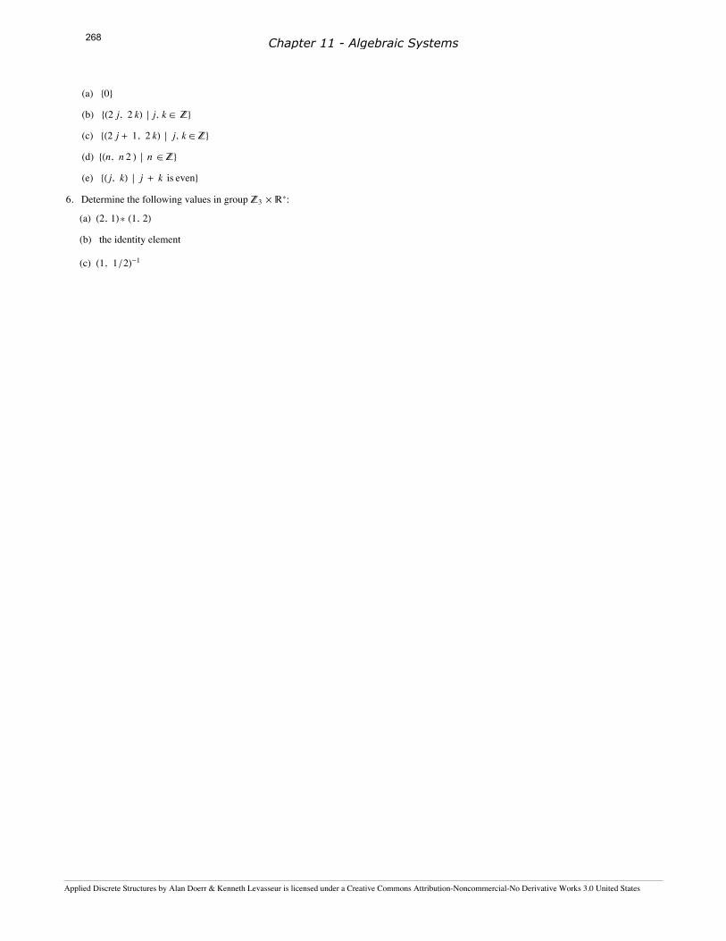
(a) 80<(b) 8H2 j, 2 kL j, k œ Z<(c) 8H2 j + 1, 2 kL j, k œ Z<(d) 8Hn, n 2 L n œ Z<(e) 8H j, kL j + k is even<

6. Determine the following values in group Z3 µ R*:

(a) H2, 1L* H1, 2L(b) the identity element

(c) H1, 1 ê2L-1



268

1.7 IsomorphismsThe following informal definition of isomorphic systems should be memorized. No matter how technical a discussion about isomorphic systemsbecomes, keep in mind that this is the essence of the concept.

Definition: Isomorphic Systems/Isomorphism. Two algebraic systems are isomorphic if there exists a translation rule between them sothat any true statement in one system can be translated to a true statement in the other

Example 11.7.1. Imagine that you are an eight-year-old child who has been reared in an English-speaking family, has moved to Greece,and has been placed in a Greek school. Suppose that your new teacher asks the class to do the following addition problem that has beenwritten out in Greek.

trίa sun tέss¶εra isoύtai ___ The natural thing for you to do is to take out your Greek-English/English-Greek dictionary and translate the Greek words to English, as

outlined in Figure 11.7.1. After you've solved the problem, you can consult the same dictionary to obtain the proper Greek word that theteacher wants. Although this is not the recommended method of learning a foreign language, it will surely yield the correct answer to theproblem. Mathematically, we may say that the system of Greek integers with addition (sun) is isomorphic to English integers with addition(plus). The problem of translation between natural languages is more difficult than this though, because two complete natural languages arenot isomorphic, or at least the isomorphism between them is not contained in a simple dictionary.

trίa sun tέss¶εra isoύtai ¶εptά

three plus four equals sevenFigure 11.7.1

Solution of a Greek arithmetic problem

Example 11.7.2. Software Implementation of Sets. In this example, we will describe how set variables can be implemented on acomputer. We will describe the two systems first and then describe the isomorphism between them.System 1: The power set of {1, 2, 3, 4, 5} with the operation union, ‹. For simplicity, we will only discuss union. However, the otheroperations are implemented in a similar way.System 2: Strings of five bits of computer memory with an OR gate. Individual bit values are either zero or one, so the elements of thissystem can be visualized as sequences of five 0's and 1's. An OR gate, Figure 11.7.2, is a small piece of computer hardware that accepts twobit values at any one time and outputs either a zero or one, depending on the inputs. The output of an OR gate is one, except when the two bitvalues that it accepts are both zero, in which case the output is zero. The operation on this system actually consists of sequentially inputtingthe values of two bit strings into the OR gate. The result will be a new string of five 0's and 1's. An alternate method of operating in thissystem is to use five OR gates and to input corresponding pairs of bits from the input strings into the gates concurrently.

System 1 :@PH81, 2, 3, 4, 5<; ‹D System 2 :Strings of 5 bits with OR

Á õ

X = 81, 2< õ 11 000Figure 11.7.2

Translation between sets and strings of bits

The Isomorphism: Since each system has only one operation, it is clear that union and the OR gate translate into one another. The translationbetween sets and bit strings is easiest to describe by showing how to construct a set from a bit string. If a1 a2 a3 a4 a5, is a bit string in System2, the set that it translates to contains the number k if and only if ak equals 1. For example, 10 001 is translated to the set 81, 5<, while the set81, 2< is translated to 11 000. Now imagine that your computer is like the child who knows English and must do a Greek problem. To executea program that has code that includes the set expression 81, 2< ‹ 81, 5<, it will follow the same procedure as the child to obtain the result, asshown in Figure 11.7.3.

81,2< ‹ 81,5< = 81,2,5<

11000 OR 10001 = 11001Figure 11.7.3

Translation of a problem in set theory

Example 11.7.3. Multiplying without doing multiplication. This isomorphism is between @R+ ; ÿD and [R;+]. Until the 1970s, when theprice of calculators dropped, multiplication and exponentiation were performed with an isomorphism between these systems. The isomor-phism HR+ to R) between the two groups is that ÿ is translated into + and any positive real number a is translated to the logarithm of a. Totranslate back from R to R+ , you invert the logarithm function. If base ten logarithms are used, an element of R, b, will be translated to 10b.In pre-calculator days, the translation was done with a table of logarithms or with a slide rule. An example of how the isomorphism is usedappears in Figure 11.7.4.



269

8 ÿ 125 = 1000

0.90309 + 2.09691 = 3.000000Figure 11.7.4

Multiplication using logarithms

The following definition of an isomorphism between two groups is a more formal one that appears in most abstract algebra texts. At firstglance, it appears different, it is really a slight variation on the informal definition. It is the common definition because it is easy to apply; thatis, given a function, this definition tells you what to do to determine whether that function is an isomorphism.

Procedure for showing that two groups are isomorphicDefinition: Group Isomorphism. If @G1 ; *1D and @G2 ; *2D are groups, f : G1 Ø G2 is an isomorphism from G1 into G2 if:

(a) f is a bijection, and

(b) f Ha *1 bL = f HaL *2 f HbL for all a, b œ G1

If such a function exists, then G1 is isomorphic to G2.

Notes:

(a) There could be several different isomorphisms between the same pair of groups. Thus, if you are asked to demonstrate that two groupsare isomorphic, your answer need not be unique.(b) Any application of this definition requires a procedure outlined in Figure 11.7.5.

Define a function T:G1ØG2 andprove that T is an isomorphism.

Prove that Tis a bijection.

Prove thatTHa *1 bL= THaL *2 THbL for all a,b œ G1.

Prove that Tis onto.

Prove that Tis one-to-one.

Figure 11.7.5Steps in proving that G1and G2 are isomorphic

The first condition, that an isomorphism be a bijection, reflects the fact that every true statement in the first group should have exactly onecorresponding true statement in the second group. This is exactly why we run into difficulty in translating between two natural languages. Tosee how Condition (b) of the formal definition is consistent with the informal definition, consider the Function L : R+ Ø R defined byL HxL = log10 x. The translation diagram between R+ and R for the multiplication problem a ÿ b appears in Figure 11.7.6. We arrive at thesame result by computing L-1 HLHaL + LHbLL as we do by computing a ÿ b. If we apply the function L to the two results, we get the sameimage: LHa ÿ bL = LHL-1HLHaL + L HbLLL = LHaL + L HbL (11.7a)

since LHL-1HxLL = x. Note that 11.7a is exactly Condition b of the formal definition applied to the two groups R+ and R.



270

a ÿ b = L-1HLHa * bLL

LHaL + LHbL = LHaÿbLFigure 11.7.6

Multiplication using logarithms - general situation

Example 11.7.4. Consider G = :K 1 a0 1 O a œ R> with matrix multiplication. This group @R; +D is isomorphic to G. Our translation rule is

the function f : R Ø G defined by f HaL = K 1 a0 1 O. Since groups have only one operation, there is no need to state explicitly that addition is

translated to matrix multiplication. That f is a bijection is clear from its definition. If a and b are any real numbers,

f HaL f HbL = K 1 a0 1 O K 1 b

0 1 O= K 1 a + b

0 1 O= f Ha + bL

We can apply this translation rule to determine the inverse of a matrix in G. We know that a + H-aL = 0 is a true statement in R. Using f totranslate this statement, we get

f HaL f H-aL = f H0Lor

K 1 a0 1 O K 1 -a

0 1 O = K 1 00 1 O

therefore,

K 1 a0 1 O-1 = K 1 -a

0 1 OTheorem 11.7.1 summarizes some of the general facts about group isomorphisms that are used most often in applications. We leave the proofto the reader.

Theorem 11.7.1. If @G;*D and @H, ùD are groups with identities e and e', respectively, and T : G Ø H is an isomorphism from G intoH, then:

(a) T HeL = e ',(b) THaL-1 = TIa-1M for all a œ G, and(c) If K is a subgroup of G, then T HKL = 8T HaL : a œ K< is a subgroup of H and is isomorphic to K.

"Is isomorphic to" is an equivalence relation on the set of all groups. Therefore, the set of all groups is partitioned into equivalence classes, eachequivalence class containing groups that are isomorphic to one another.

Procedures for showing groups are not isomorphicHow do you decide that two groups are not isomorphic to one another? The negation of "G and H are isomorphic" is that no translation rulebetween G and H exists. If G and H have different cardinalities, then no bijection from G into H can exist. Hence they are not isomorphic.Given that †G§ = †H§, it is usually impractical to list all bijections from G into H and show that none of them satisfy Condition b of the formaldefinition. The best way to prove that two groups are not isomorphic is to find a true statement about one group that is not true about the othergroup. We illustrate this method in the following checklist that you can apply to most pairs of non-isomorphic groups in this book.Assume that @G;*D and @H;ùD are groups. The following are reasons for G and H to be not isomorphic.

(a) G and H do not have the same cardinality. For example, Z12 µ Z5 can't be isomorphic to Z50 and @R; +D can't be isomorphic to @Q+ ; ÿD,(b) G is abelian and H is not abelian since a * b = b * a is always true in G, but T HaL ù T HbL = T HbL ù T HaL would not always be true. Twogroups with six elements each are Z6 and the set of 3 µ 3 rook matrices (see Exercise 5 in Section 11.2). The second group is non-abelian,therefore it can't be isomorphic to Z6 .(c) G has a certain kind of subgroup that H doesn't have. Theorem 11.7.1(c) states that this cannot happen if G is isomorphic to H. @R* ; ÿD and@R+ ; ÿD are not isomorphic since R* has a subgroup with two elements, 8-1, 1<, while the proper subgroups of R+ are all infinite (Convinceyourself of this fact!).(d) The number of solutions of x * x = e in G is not equal to the number of solutions of y ù y = e ' in H. Z8 is not isomorphic to Z23 sincex +8 x = 0 has two solutions, 0 and 4, while y + y = H0, 0, 0L is true for all y œ Z2

3. If the operation in G is defined by a table, then thenumber of solutions of x * x = e will be the number of occurrences of e in the main diagonal of the table. The equations x3 = e, x4 = e, …can also be used in the same way to identify non-isomorphic groups.(e) One of the cyclic subgroups of G equals G (i. e., G is cyclic), while none of H's cyclic subgroups equals H (i. e., H is noncyclic). This is aspecial case of Condition c. Z and Z µ Z are not isomorphic since Z = X1\ and Z µ Z is not cyclic.



271

EXERCISES FOR SECTION 11.7A Exercises1. State whether each pair of groups below is isomorphic. If it is, give an isomorphism; if it is not, give your reason.

(a) Z µ R and R µ Z

(b) Z2µZ and Z µ Z

(c) R and Q µ Q

(d) PH81, 2<L with symmetric difference and Z22

(e) Z22 and Z4

(f) R4 and M2µ2HRL with matrix addition

(g) R2 and R µ R+ (h) Z2 and the 2 µ 2 rook matrices

(i) Z6 and Z2µ Z3

2. If you know two natural languages, show that they are not isomorphic.

3. Prove that the relation "is isomorphic to" on groups is transitive.

4. (a) Write out the operation table for G = @81, — 1, Â, -Â<, ÿD where Â is the complex number for which Â2 = - 1. Show that G is isomor-phic to @Z4; +4D. (b) Solve x2 = -1 in G by first translating to Z4 , solving the equation in Z4 , and then translating back to G.

B Exercises5. It can be shown that there are five non-isomorphic groups of order eight. You should be able to describe at least three of them. Do sowithout use of tables. Be sure to explain why they are not isomorphic.6. Prove Theorem 11.7.1.

7. Prove that all infinite cyclic groups are isomorphic to Z.

8. (a) Prove that R* is isomorphic to Z2 µ R.

(b) Describe how multiplication of nonzero real numbers can be accomplished doing only additions and translations.

9. Prove that if G is any group and g is some fixed element of G, then the function fg defined by fgHxL = g* x*g-1 is an isomorphism from Ginto itself. An isomorphism of this type is called an automorphism.



272

11.8 Using Computers to Study Groups

Groups in MathematicaMathematica has a wide variety of computable databases available and one of them is on finite groups. To access the database you use thefunction FiniteGroupData. Extensive documentation is available at . Since we've only scratch the surface of group theory at this point,most of the groups and concepts mentioned are likely to be unfamiliar to the reader. For this reason, we well wait until Chapter 15 to discussthat database.The Combinatorica package that is included in all Mathematica distributions has limited abstract algebra

<< Combinatorica`

Here is how to generate the body of the operation table for the ring @Z7; +7D. Notice that this really an addition table even though the functionthat creates the table is called MultiplicationTable.

MultiplicationTable@Range@0, 6D, Function@8a, b<, Mod@a + b, 7DDD1 2 3 4 5 6 72 3 4 5 6 7 13 4 5 6 7 1 24 5 6 7 1 2 35 6 7 1 2 3 46 7 1 2 3 4 57 1 2 3 4 5 6

An even more user-friendly package that you would need to download to use is available at Exploring Abstract Algebra with Mathematica(http://www.central.edu/EAAM/). The package, when installed on your computer, is loaded with the command

<< AbstractAlgebra`Master`

The group Z12 is

G = ZG@12DGroupoidH80, 1, 2, 3, 4, 5, 6, 7, 8, 9, 10, 11<, HÒ1 + Ò2L mod 12 &L

At this point G is an object that consists of the set 80, 1, 2, …, 11< and the binary operation +12. Among things we can do with G is that we can

examine its subgroups.Subgroups@GD8GroupoidH80<, HÒ1 + Ò2L mod 12 &L, GroupoidH80, 2, 4, 6, 8, 10<, HÒ1 + Ò2L mod 12 &L,

GroupoidH80, 3, 6, 9<, HÒ1 + Ò2L mod 12 &L, GroupoidH80, 4, 8<, HÒ1 + Ò2L mod 12 &L,GroupoidH80, 6<, HÒ1 + Ò2L mod 12 &L, GroupoidH80, 1, 2, 3, 4, 5, 6, 7, 8, 9, 10, 11<, HÒ1 + Ò2L mod 12 &L<

We can view the inverses of elements in a variety of ways. For example, we can get them paired up. Notice that two of the elements, 0 and 6invert themselves.

Inverses@GD0 01 112 103 94 85 76 6

There is a "Visual Mode" that gives us a different view of the inverses. The boxes with "?" and "Ø" give further information in you are readingthis in a Mathematica Notebook and have the package installed.



273

Inverses@G, Mode Ø VisualD0

1

2

3

4

56

7

8

9

10

11

? Ø

The package was designed for teaching a first course in abstract algebra and so it has features that are more basic than other abstract algebraresources. For example, we can ask G is really a group and get quite a bit of information.



274

GroupQ@G, Mode Ø TextualDGiven a set S and an operation *, we call the pair HS,*La group if S is closed under the operation *, there is an identityelement, every elemement has an inverse and the operation * isassociative.

We say a Groupoid G has an identity e if for all other elements g in G we have e + g = g + e = g Hwhere + indicates the operationL.In this case, Z@12D has the identity 0.

Ø

We say that a set S is closed under an operation op if whenever we have x and y in S, we also have op@x,yD Hor x~op~yL in S.In this case, the Groupoid Z@12D is indeed closed.

Ø

Given a Groupoid G, we say an element g in G has an inverse h if G has an identity, say e, and g + h = h + g= e Hwhere + indicates the operationL. The Groupoid Z@12D has an inverse for every element. Here they are:

x x-10 01 112 103 94 85 76 6

Ø

Given a structured set S HGroupoid or RingoidL, we say the operation * isassociative if for every g, h, and k in S we have Hg*hL*k = g*Hh*kL, where * is the group operation.

In this case, Z@12D is associative. Consider the following table illustrating randomtriples that associate. Pay attention to the last two columns.

i j k Hi*jL*k i*Hj*kL2 11 4 5 53 1 4 8 88 9 8 1 17 5 2 2 28 8 2 6 6

10 6 9 1 14 9 7 8 84 5 2 11 11

11 4 1 4 45 10 6 9 9

Ø

This package also has much more capabilities than what we've covered so far and we will revisit it in Chapters 15 and 16.

Groups in SageAbstract Algebra seems to have been given a much higher priory in the design of Sage than it was in Mathematica. Again, the capabilities farexceed what we've touch on in the theory, but here are a few examples that you should understand. Here is how to generate the group Z14.

G=AbelianGroup(1,[14])



275

G.list()[1, f, f^2, f^3, f^4, f^5, f^6, f^7, f^8, f^9, f^10, f^11, f^12, f^13]

There is no output from assigning G. The elements of G are generated from the list method. The connection with Z14 is that when wemultiply powers of f, the exponents are added with +14. Among other things we can ask whether G is abelian and what its subgroups are.

G.is_abelian()TrueG.subgroups()[Multiplicative Abelian Group isomorphic to C2 x C7, which is thesubgroup ofMultiplicative Abelian Group isomorphic to C14generated by [f], Multiplicative Abelian Group isomorphic to C7, whichis the subgroup ofMultiplicative Abelian Group isomorphic to C14generated by [f^2], Multiplicative Abelian Group isomorphic to C2, whichis the subgroup ofMultiplicative Abelian Group isomorphic to C14generated by [f^7], Trivial Abelian Group, which is the subgroup ofMultiplicative Abelian Group isomorphic to C14generated by []]



276

SUPPLEMENTARY EXERCISES FOR CHAPTER 11Section 11.1

1. V = {a, b, c} is a set with operations + and · defined by the following "addition" and "multiplication" tables:

+ a b cabc

a b cb c ac a b

ÿ a b cabc

a a aa b ca c b

(a) With respect to V under + determine,

(i) The identity (i.e., the "zero" of the addition).

(ii) The inverse of each element, that is, -a, -b, and -c.

(b) With respect to V under · determine,

(i) The identity (i.e., the "one" of the multiplication).

(ii) The inverse of each element different from "zero."

(c) Is + distributive over · ? Is · distributive over + ?

2. (a) Determine whether the following are valid binary operations on the given sets. Explain fully.

(i) Matrix addition on A = :K a bc 0 O a, b, c œ R>

(ii) Matrix multiplication on the set A above.

(iii) On Q+, define * by a * b = Ha ÿ bL ê2.

(iv) Function composition on AA = {ƒ: A Ø A}, where A is {1, 2, 3}.

(v) Function composition on B = 8ƒ œ AA ƒ is a bijection<. (b) For each binary operation above give the identity element if it exists. Explain.

(c) Determine which of the above binary operations are commutative and which are associative.

3. Let S = set of all bijections of a set A, and let Î be function composition. Does Î have the inverse property? Does function composition havethe involution property? Explain.4. Does + on M2µ2HRL have the inverse property? Does + have the involution property? Explain.

5. Prove that the odd integers are closed under multiplication but not under addition. Are the even integers closed under both addition andmultiplication? Prove your answers.Section 11.2

6. (a) Show that R2 is a group under componentwise addition, that is, Ha1, a2L + Hb1, b2L = Ha1 + a2, b1 + b2L. (b) Show that 8Hx, 2 xL x œ R< is a group under componentwise addition. Draw the graph of this subset. Describe similarsubsets of R2 that are also groups.7. Prove that the set of all 2 µ 2 invertible matrices (over R) is a group under matrix multiplication. Assume, as indicated in Chapter 5, that theassociative law is true for matrices under multiplication. This group is called the general linear group of degree 2 over R, and it is denoted byGLH2, RL. It is given this name because these matrices are matrix representations of linear motions of R2 .

8. Prove that :A = K a bc d O det A = 1> is a group under matrix multiplication. Assume that the associative law is true under matrix multi-

plication. This group is called the special linear group of degree 2 over R and it is denoted SLH2, RL.9. Show that R is a group under the operation * defined by a * b = a + b + 5 for a, b œ R.

10. (a) let B3µ3 be the set of all 3 µ 3 Boolean (adjacency) matrices discussed in Section 6.4. Is B3µ3 a monoid under Boolean addition? Is it agroup? Explain. (b) Is B3µ3 a monoid under Boolean multiplication? Is it a group? Explain.

Section 11.3


277

11. Define * on Q+ by a * b = Ha bL ê2. Prove that @Q+ ; *D is a group.

12. Let G be the group R under the operation a * b = a + b + 5 for a, b œ R. Solve the following equations for x in G.

(a) x * 3 = 5 (d) x2 = 2

(b) 2 * x * 4 = 6 (e) 4 * x2 = 5

(e) x3 = 713. Solve the equation A *X * B = C in GLH2, RL where

A = K 2 00 3 O, B = K 4 2

2 2 O, and C = K 2 10 1 O.

14. Prove that if @G; *D is a group, Ha * bLn = an * bn for all n ¥ 1 and a, b œ G if and only if [G;*] is an abelian group.

Section 11.4

15. Calculate the following in Z5:

(a) 3 +5 8

(b) H-3L µ5 2

(c) H3 µ5 2L +5 H2 µ5 2L (d) 2 -1 (i.e., the multiplicative inverse of 2)16. (a) Prove that {1, 3, 5, 7}, is a group under µ8 . Write out its group table.

(b) Let U HZnL stand for the elements of Zn , which have inverses under µn. Convince yourself that UHZn L is a group under µn.

(c) Prove that the elements of UHZn L are those elements a œ Zn such that gcdHa, nL = 1. You may use the fact that gcdHa, bL = 1 ñthere exist integers s and t such that sa + tb = 1.Section 11.5

17. (a) Recall from "Supplementary Exercises," Section 11.4, that UHZ8 Lis a group under µ8 . List all cyclic subgroups of this group.

(b) Is UHZ8 L a cyclic group? Explain.

18. (a) Use Theorem 11.5.1 to prove that the set of even integers is a subgroup of the group Z (under +).

(b) Is the set of odd integers a subgroup of the group Z (under +)?

19. Prove that SLH2, RL is a subgroup of GLH2, RL. See Exercises 7 and 8 above for an explanation of this notation.

20. Recall that M2µ2HRL is a group under addition.

(a) Is A = :K a ba 0 O a, b œ R> a subgroup of M2µ2 HRL?

(b) Is B = :K a bb 1 O a, b œ R> a subgroup of M2µ2 HRL?

(c) Are either of the subsets in parts a and b subgroups of GLH2, RL?21. Let B3µ3 be the monoid of all 3 µ 3 Boolean matrices, under Boolean addition. Let S be a subset of B3µ3 consisting of all 3 µ 3 matricesthat represent symmetric relations. Is S a submonoid of B3µ3 ?Section 11.6

22. Using the data structure in the text for doubly linked lists with six-bit addresses, what are the addresses of the records containing A and D?Write your answer as a sum in the group Z26 and then as an address.

A

?

B

010101

011100

C

001011

000011

D

?

23. Determine the inverse of each element in the respective group.

(a) (2, 3, 5) in Z3 µ Z7 µ Z25

(b) (1,0, 1, l) in Z4



278

(c) (3, 2) in R+ µ Z6

(d) (2, 3,5) in R3

24. Determine the identity elements in the following groups:

(a) R+µR+

(b) R+µZ3

(c) GLH2, RL µ R3

25. Which of the following groups are abelian? Explain.

(a) Z2µZ24µZ75

(b) GLH2, RL µZ2

(c) Zn

26. Is 80, 3< µ 80, 4, 8< a subgroup of Z6 µ Z8 ? Explain.

Section 11.7

27. Prove that the cyclic subgroup (4) of Z16 is isomorphic to Z4 .

28. Let G = 8 &, $, %<. Given that @G; *D is a group and that it is isomorphic to the group @Z3; +3D with isomorphism T : G Ø Z3 definedby T H &L = 1, T H$L = 2, and T H%L = 0. What are (a) $ * $ (b) The identity of @G; *D29. Let U be a set and PU = {propositions over the set U}. It can be shown that the algebraic system @PU; ~, Ô , ÓD is isomorphic to@PHUL; ÿ, ›, ‹D. (a) Explain what this means.

(b) How does this help you understand the language of the algebra of propositions?

(c) Give the "propositional" analogue to the following statement: If A › Bc = « and A › B = « then A = «.30. Write out the operation tables for the following systems:

(a) [{0, 1}; +, ·] where + and · denote Boolean addition and multiplication.

(b) @8-1, 1<; Ô, ÓD where i Ô j and i Ó j denote the largest and smallest, respectively, of i and j.

(c) @Z2; +2, µ2D. Are these systems isomorphic? Explain.

31. Prove that the group C, under +, is isomorphic to the group R2 , under + .32. Determine which of the following groups are isomorphic. Explain.

(a) R3 , the 3 µ 3 rook matrices, and Z6

(b) R3 and SA = 8 f œ AA : ƒ is a bijection<, where A is {1, 2, 3}. (c) Z6 and UHZ7L33. Prove that R4 under addition, is isomorphic to M2µ2HRL, under addition.34. Prove that the group @UHZ8L; µ8D is isomorphic to @Z4; +4 D.



279

chapter 12

MORE MATRIX ALGEBRA

GOALSIn Chapter 5 we studied matrix operations and the algebra of sets and logic. We also made note of the strong resemblance of matrix algebra toelementary algebra. The reader should briefly review this material. In this chapter we shall look at a powerful matrix tool in the appliedsciences—namely, a technique for solving systems of linear equations. We will then use this process for determining the inverse of nµnmatrices, n ¥ 2, when they exist. We conclude by a development of the diagonalization process, with a discussion of several of its applications.

12.1 Systems of Linear EquationsThe method of solving systems of equations by matrices that we will look at is based on procedures involving equations that we are familiarwith from previous mathematics courses. The main idea is to reduce a given system of equations to another simpler system that has the samesolutions.

Definition: Solution Set. Given a system of equations involving real variables x1, x2, …, xn, the solution set of the system is the set of n-tuples in Rn, Ha1, a2, …, anL such that the substitutions x1 = a1, x2 = a2, …, xn = an make all the equations true.In general, if the variables are from a set S, then the solution set will be a subset of Sn. For example, in number theory mathematicians studyDiaphanine equations, where the variables can only take on integer values instead of real values.

Definition: Equivalent Systems of Equations. Two systems of linear equations are called equivalent if they have the same set ofsolutions.

Example 12.1.1. The previous definition tells us that if we know that the system

4 x1 + 2 x2 + x3 ‡ 12 x1 + x2 + x3 ‡ 42 x1 + 2 x2 + x3 ‡ 3

is equivalent to the system

x1 + 0 x2 + 0 x3 ‡ -10 x1 + x2 + 0 x3 ‡ -10 x1 + 0 x2 + x3 ‡ 7

then both systems have the solution set 8H-1, -1, 7L<. In other words, the values x1 = -1, x2 = -1, and x3 = 7 are the only values of thevariables that make all three equations in either system true.

Theorem 12.1.1. Elementary Operations on Equations. If any sequence of the following operations is performed on a system ofequations, the resulting system is equivalent to the original system:(1) Interchange any two equations in the system.

(2) Multiply both sides of any equation by a nonzero constant.


280

(3) Multiply both sides of any equation by a nonzero constant and add the result to a second equation in the system, with the sum replacingthe latter equation.Let us now use the above theorem to work out the details of Example 12.1.1 and see how we can arrive at the simpler system..

Step 1. We will first change the coefficient of x1 in the first equation to one and then use it as a pivot to obtain 0's for the coefficients of x1 inEquations 2 and 3.

H1.1L 4 x1 + 2 x2 + x3 ‡ 12 x1 + x2 + x3 ‡ 42 x1 + 2 x2 + x3 ‡ 3

Multiply Equation 1 by 14

to obtain

H1.2L x1 +x22+ x3

4‡ 1

42 x1 + x2 + x3 ‡ 42 x1 + 2 x2 + x3 ‡ 3

Multiply Equation 1 by - 2 and

add the result to Equation 3 to obtain

H1.3Lx1 + x2

2+ x3

4‡ 1

4

0 x1 + 0 x2 +x32

‡ 72

2 x1 + 2 x2 + x3 ‡ 3

Multiply Equation 1 by - 2 and add

the result to Equation 3 to obtain

H1.4Lx1 + x2

2+ x3

4‡ 1

4

0 x1 + 0 x2 +x32

‡ 72

0 x1 + x2 +x32

‡ 52

Note: We've explicitly written terms with zero coefficients such as 0 x1 to make a point that all variables can be thought of as beinginvolved in all equations. After this example we will discontinue this practice in favor of the normal practice of making these terms"disappear."Step 2. We would now like to proceed in a fashion analogous to Step 1—namely, multiply the coefficient of x2 in the second equation by asuitable number so that the result is 1. Then use it as a pivot to obtain 0's as coefficients for x2 in the first and third equations. This is clearlyimpossible (Why?), so we will first interchange Equations 2 and 3 and proceed as outlined above.

H2.1Lx1 + x2

2+ x3

4‡ 1

4

0 x1 + 0 x2 +x32

‡ 72

0 x1 + x2 +x32

‡ 52

Interchange Equations 2 and 3 to obtain

H2.2Lx1 + x2

2+ x3

4‡ 1

4

0 x1 + x2 + x32

‡ 52

0 x1 + 0 x2 +x32

‡ 72

Multiply Equation 2 by - 12

and addthe result to Equation 1 to obtain

(2.3)

x1 + 0 x2 + 0 x3 ‡ -1

0 x1 + x2 + x32

‡ 52

0 x1 + 0 x2 + x32

‡ 72

Step 3. Next, we will change the coefficient of x3 in the third equation to one and then use it as a pivot to obtain 0's for the coefficients of x3 inEquations 1 and 2.

(3.1)

x1 + 0 x2 + 0 x3 ‡ -1

0 x1 + x2 + x32

‡ 52

0 x1 + 0 x2 + x32

‡ 72

Multiply Equation 3 by 2 to obtain

(3.2)

x1 + 0 x2 + 0 x3 ‡ -1

0 x1 + x2 + x32

‡ 52

0 x1 + 0 x2 + x3 ‡ 7

Multiply Equation 3 by - 12

and add the resultto Equation 2 to obtain

(3.3) x1 + 0 x2 + 0 x3 ‡ -1

0 x1 + x2 + 0 x3 ‡ -10 x1 + 0 x2 + x3 ‡ 7

Chapter 12 - More Matrix Algebra


281

From the system of equations in Step 3.3, we see that the solution to the original system (Step 1.1) is x1 = -1, x2 = -1, and x3 = 7 .

In the above sequence of steps, we note that the variables serve the sole purpose of keeping the coefficients in the appropriate location. This wecan effect by using matrices. The matrix of the system given in Step 1.1 is

4 2 1 12 1 1 42 2 1 3

where the matrix of the first three columns is called the coefficient matrix and the complete matrix is referred to as the augmented matrix. Sincewe are now using matrices to solve the system, we will translate Theorem 12.1.1 into matrix language.

Definition: Elementary Row Operations. The following operations on a matrix are called elementary row operations:

(1) Interchange any two rows of the matrix.

(2) Multiply any row of the matrix by a nonzero constant.

(3) Multiply any row of the matrix by a nonzero constant and add the result to a second row, with the sum replacing the second row.

Definition: Row Equivalent. Two matrices, A and B, are said to be row-equivalent if one can be obtained from the other by any oneelementary row operation or by any sequence of elementary row operations.If we use the notation Ri to stand for Row i of a matrix and ö to stand for row equivalence, then

Ac Ri+ R j

Bmeans that the matrix B is obtained from the matrix A by multiplying the Row i of A by c and adding the result to Row j. The operation ofmultiplying row i by c is indicated by

A öc Ri B

while interchanging rows i and j is denoted by

ARi¨R j

B.The matrix notation for the system given in Step 1.1 with the subsequent steps are:

4 2 1 12 1 1 42 2 1 3

ö

1

4R1

1 12

14

14

2 1 1 42 2 1 3

ö-2 R1+ R2

1 12

14

14

0 0 12

72

2 2 1 3

ö-2 R1+ R3

1 12

14

14

0 0 12

72

0 1 12

52

öR2¨R3

1 12

14

14

0 1 12

52

0 0 12

72

ö-1

2R2+ R1

1 0 0 -1

0 1 12

52

0 0 12

72

ö2 R3

1 0 0 -1

0 1 12

52

0 0 1 7

ö-1

2R3+ R2

1 0 0 -10 1 0 -10 0 1 7

This again gives us the solution. This procedure is called the Gauss-Jordan elimination method.

It is important to remember when solving any system of equations via this or any similar approach that at any step in the procedure we canrewrite the matrix in "equation format" to help us to interpret the meaning of the augmented matrix.In Example 12.1.1 we obtained a unique solution, only one triple, namely H-1, -1, 7L, which satisfies all three equations. For a systeminvolving three unknowns, are there any other possible results? To answer this question, let's review some basic facts from analytic geometry.The graph of a linear equation in three-dimensional space is a plane. So geometrically we can visualize the three linear equations as three planesin three-space. Certainly the three planes can intersect in a unique point, as in Example 12.1.1, or two of the planes could be parallel. If twoplanes are parallel, there are no common points of intersection; that is, there are no triple of real numbers that will satisfy all three equations.Also, the three planes could intersect along a common axis or line. In this case, there would be an infinite number of real number triples in R3that would satisfy all three equations. Finally if all three equations describe the same plane, the solution set would be that plane. Wegeneralize;



282

In a system of n linear equations, n unknowns, there can be:

(1) a unique solution,

(2) no solution, or

(3) an infinite number of solutions.

To illustrate these points, consider the following examples:

Example 12.1.2. Find all solutions to the system

x1 + 3 x2 + x3 ‡ 2x1 + x2 + 5 x3 ‡ 4

2 x1 + 2 x2 + 10 x3 ‡ 6The reader can verify that the augmented matrix of this system,

1 3 1 21 1 5 42 2 10 6

,

reduces to

1 3 1 21 1 5 40 0 0 -2

(See exercise 4 of this section.)

We can row-reduce this matrix further if we wish. However, any further row-reduction will not substantially change the last row, which, inequation form, is 0 x1 + 0 x2 + 0 x3 = -2, or simply 0 = -2. It is clear that we cannot find real numbers x1, x2, and x3 that will satisfy thisequation, hence we cannot find real numbers that will satisfy all three original equations simultaneously. When this occurs, we say that thesystem has no solution, or the solution set is empty.

Example 12.1.3. Next let's attempt to find all of the solutions to:

x1 + 6 x2 + 2 x3 ‡ 12 x1 + x2 + 3 x3 ‡ 24 x1 + 2 x2 + 6 x3 ‡ 4

The augmented matrix for the system,

1 6 2 12 1 3 24 2 6 4

reduces to

1 0 1611

1

0 1 111

00 0 0 0

If we apply additional elementary row operations to this matrix, it will only become more complicated. In particular, we cannot get a one inthe third row, third column. Since the matrix is in simplest form, we will express it in equation format to help us determine the solution set.

x1 + 1611

x3 ‡ 1

x2 +111

x3 ‡ 00 = 0

Any real numbers will satisfy the last equation. However, the first equation can be rewritten as x1 = 1 - 1611

x3, which describes the coordi-nate x1 in terms of x3 . Similarly, the second equation gives x1in terms of x3 . A convenient way of listing the solutions of this system is to useset notation. If we call the solution set of the system S, then

S = 9I1 - 1611

x3, - 111

x3, x3M x3 œ R=.What this means is that if we wanted to list all solutions, we would replace x3 by all possible numbers. Clearly, there is an infinite number ofsolutions, two of which are H1, 0, 0L and H-15, -1, 11L.

A Word Of Caution: Frequently we may obtain “different-looking” answers to the same problem when a system has an infinite numberof answers. Assume a student’s solutions set to Example 12.1.3 is A = 8H1 + 16 x2, x2, -11 x3L x3 œ R<. Certainly the result described byS looks different from that described by A. To see whether they indeed describe the same set, we wish to determine whether every solutionproduced in S can be generated in A. For example, the solution generated by S when x3 = 11 is H-15, -1, 11L. The same triple can beproduced by A by taking x2 = -1. We must prove that every solution described in S is described in A and, conversely, that every solutiondescribed in A is described in S. (See Exercise 6 of this section.)



283

To summarize the procedure in the Gauss-Jordan technique for solving systems of equations, we attempt to obtain 1’s along the main diagonalof the coefficient matrix with 0’s above and below the diagonal, as in Example 12.1.1. We may find in attempting this that the closest we cancome is to put the coefficient matrix in "simplest" form, as in Example 12.1.3, or we may find that the situation of Example 12.1.1 evolves aspart of the process. In this latter case, we can terminate the process and state that the system has no solutions. The final matrix forms ofExamples 12.1.1 and 12.1.3 are called echelon forms.In practice, larger systems of linear equations are solved using computers. Generally, the Gauss-Jordan algorithm is the most useful; however,slight variations of this algorithm are also used. The different approaches share many of the same advantages and disadvantages. The two majorconcerns of all methods are:(1) minimizing inaccuracies due to rounding off errors, and

(2) minimizing computer time.

The accuracy of the Gauss-Jordan method can be improved by always choosing the element with the largest absolute value as the pivot element,as in the following algorithm.

Algorithm 12.1.1. Given a matrix equation A x = b, where A is n × m, let C be the augmented matrix @A bD. The process of row-reducing to eschelon form involves performing the following algorithm where Ci = the ith row of C:

i = 1j = 1while (i § n and j § m): # Find pivot in column j, starting in row i: maxi = i for k = i+1 to n: if abs(C[k,j]) > abs(C[maxi,j]) then maxi := k if C[maxi,j] ¹≠ 0 then interchange rows i and maxi divide each entry in row i by C[i,j] # Now C[i,j] will have the value 1. for u = i+1 to n: subtract C@u, jD * Ci from Cu # Now C[u,j] will be 0 i := i + 1 end if j = j + 1end while

At the end of this algorithm, with the final form of C you can revert back to the equation form of the system and a solution should be clear. Ingeneral,(a) If any row of C is all zeros, it can be ignored.(b) If any row of C has all zero entries except for the entry in the Hm + 1Lst position, the system has no solution. Otherwise, if a column hasno pivot, the variable corresponding to it is a free variable. Variables corresponding to pivots are basic variables and can be expressed interms of the free variables.

Example 12.1.4. If we apply Algorithm 12.1.1 to the system

5 x1 + x2 + 2 x3 + x4 ‡ 23 x1 + x2 - 2 x3 ‡ 5

x1 + x2 + 3 x3 - x4 ‡ -1the augmented matrix

C =5 1 2 1 23 1 -2 0 51 1 3 -1 -1

is reduced to a new value of C:

C =

1 0 0 12

12

0 1 0 - 32

32

0 0 1 0 -1therefore x4 is a free variable in the solution and general solution of the system is



284

x =

x1x2x3x4

=

12- 12

x432+ 32

x4-1x4

This conclusion is easy to see if you revert back to the equations that the final value matrix C represents.

Mathematica Note

The Mathematica function RowReduce does the same reduction as described in Algorithm 12.1.1. For example, here is the result for thesystem in Example 12.1.4.

RowReduceB 5 1 2 1 23 1 -2 0 51 1 3 -1 -1

F1 0 0 1

212

0 1 0 - 32

32

0 0 1 0 -1

Options@RowReduceD8Method Ø Automatic, Modulus Ø 0, Tolerance Ø Automatic, ZeroTest Ø Automatic<

Only one caution: One needs to be aware that if the pivoting process continues into the last column, which Mathematica will do, there will notbe a solution to the system. For example the system

2 x1 - x2 ‡ 13 x2 - x1 ‡ 5x1 + 5 x2 ‡ 7

has augmented matrix

C =2 -1 1-1 3 51 5 7

.

Here is the computation to row-reduce:

RowReduceB 2 -1 1-1 3 51 5 7

F1 0 00 1 00 0 1

The last row of the final form of C is 0 = 1 and so there is no solution to the original system.

Sage Note

Given an augmented matrix, C, there is a matrix method called eschelon_form that can be used to row reduce C. Here is the result for thesystem in Example 12.1.4. In the assignment of a matrix value to C, notice that the first argument is QQ, which indicates that the entriesshould be rational numbers. As long as all the entries are rational, which is the case here since integers are rational, the row-reduced matrixwill be all rational.

C = Matrix(QQ,[[5,1,2,1,2],[3,1,-2,0,5],[1,1,3,-1,-1]])C.echelon_form()

[ 1 0 0 1/2 1/2][ 0 1 0 -3/2 3/2][ 0 0 1 0 -1]

If we didn't specify the set from which entries are taken, it would assumed to be the integers and we would not get a fully row-reduced matrix.The next step would involve multiplying row 3 by 1

9, which isn't an integer.

C2 = Matrix([[5,1,2,1,2],[3,1,-2,0,5],[1,1,3,-1,-1]])C2.echelon_form()



285

_

[ 1 1 3 -1 -1][ 0 2 2 -3 1][ 0 0 9 0 -9]

This is why we would avoid specifying real entries:

C3 = Matrix(RR,[[5,1,2,1,2],[3,1,-2,0,5],[1,1,3,-1,-1]])C3.echelon_form() [ 1.00000000000000 0.000000000000000 0.000000000000000 0.500000000000000 0.500000000000000][ 0.000000000000000 1.00000000000000 0.000000000000000 -1.50000000000000 1.50000000000000][ 0.000000000000000 0.000000000000000 1.00000000000000 4.93432455388958e-17 -1.00000000000000]

This is the default number of decimal places, which could be controled and the single small number in row three column four isn't exactly zerobecause of round-off and we could just set it to zero. However, the result isn't as nice and clean as the rational output in this case.

EXERCISES FOR SECTION 12.1A Exercises1. Solve the following systems by describing the solution sets completely:

(a) 2 x1 + x2 ‡ 3x1 - x2 ‡ 1

(b) 2 x1 + x2 + 3 x3 ‡ 54 x1 + x2 + 2 x3 ‡ -18 x1 + 2 x2 + 4 x3 ‡ -2

(c) x1 + x2 + 2 x3 ‡ 1x1 + 2 x2 - x3 ‡ -1x1 + 3 x2 + x3 ‡ 5

(d) x1 - x2 + 3 x3 ‡ 7x1 + 3 x2 + x3 ‡ 4

2. Solve the following systems by describing the solution sets completely:

(a) 2 x1 + 2 x2 + 4 x3 ‡ 22 x1 + x2 + 4 x3 ‡ 03 x1 + 5 x2 + x3 ‡ 0

(b) 2 x1 + x2 + 3 x3 ‡ 24 x1 + x2 + 2 x3 ‡ -18 x1 + 2 x2 + 4 x3 ‡ 4

(c) x1 + x2 + 2 x3 + x4 ‡ 3x1 - x2 + 3 x3 - x4 ‡ -23 x1 + 3 x2 + 6 x3 + 3 x4 ‡ 9

(d) 6 x1 + 7 x2 + 2 x3 ‡ 34 x1 + 2 x2 + x3 ‡ -26 x1 + x2 + x3 ‡ 1

(e) x1 + x2 - x3 + 2 x4 ‡ 1x1 + 2 x2 + 3 x3 + x4 ‡ 5x1 + 3 x2 + 2 x3 - x4 ‡ -1

3. Given that the final augmented matrices below obtained from Algorithm 12.1.1, identify the solutions sets. Identify the basic and freevariables, and describe the solution set of the original system.

(a) 1 0 -5 0 1.20 1 4 0 2.60 0 0 1 4.5

(c) 1 0 9 30 1 0 40 0 0 1

(b) 1 0 6 50 1 -2 10 0 0 0

(d) 1 0 0 -3 10 1 0 2 20 0 1 -1 1



286

4. (a) Write out the details of Example 12.1.2.

(b) Write out the details of Example 12.1.3.

(c) Write out the details of Example 12.1.4.

5. Solve the following systems using only mod 5 arithmetic. Your solutions should be n - tuples from Z5.

(a) 2 x1 + x2 ‡ 3x1 + 4 x2 ‡ 1 (compare your solution to the system in 5(a))

(b) x1 + x2 + 2 x3 ‡ 1x1 + 2 x2 + 4 x3 ‡ 4x1 + 3 x2 + 3 x3 ‡ 0

6. (a) Use the solution set S of Example 12.1.3 to list three different solutions to the given system. Then show that each of these solutions can bedescribed by the set A of Example 12.1.3. (b) Prove that S = A.

B Exercise7. Given a system of n linear equations in n unknowns in matrix form A x = b, prove that if b is a matrix of all zeros, then the solution set ofA x = b is a subgroup of Rn .

12.2 Matrix InversionIn Chapter 5 we defined the inverse of an n µ n matrix. We noted that not all matrices have inverses, but when the inverse of a matrix exists, itis unique. This enables us to define the inverse of an n × n matrix A as the unique matrix B such that A B = B A = I, where I is the n µ nidentity matrix. In order to get some practical experience, we developed a formula that allowed us to determine the inverse of invertible 2µ2matrices. We will now use the Gauss-Jordan procedure for solving systems of linear equations to compute the inverses, when they exist, of nµnmatrices, n ¥ 2. The following procedure for a 3µ3 matrix can be generalized for nµn matrices, n ¥ 2.Example 12.2.1. Given the matrix

A =1 1 22 1 43 5 1

we want to find the matrix

B =x11 x12 x13x21 x22 x23x31 x32 x33

,

if it exists, such that (a) A B = I and (b) B A = I. We will concentrate on finding a matrix that satisfies Equation (a) and then verify that B alsosatisfies Equation (b).

1 1 22 1 43 5 1

x11 x12 x13x21 x22 x23x31 x32 x33

=1 0 00 1 00 0 1

is equivalent to

x11 + x21 + 2 x31 x12 + x22 + 2 x32 x13 + x23 + 2 x33

2 x11 + x21 + 4 x31 2 x12 + x22 + 4 x32 2 x13 + x23 + 4 x333 x11 + 5 x21 + x31 3 x12 + 5 x22 + x32 3 x13 + 5 x23 + x33

=1 0 00 1 00 0 1

(12.2.a)

By definition of equality of matrices, this gives us three systems of equations to solve. The augmented matrix of one of the 12.2a systems, theone equating the first columns of the two matrices is:

1 1 2 12 1 4 03 5 1 0

(12.2.b)

Using the Gauss-Jordan technique of Section 12.1, we have:



287

1 1 2 12 1 4 03 5 1 0

ö-2 R1+R2

1 1 2 10 -1 0 -23 5 1 0

ö-3 R1+R3

1 1 2 10 -1 0 -20 2 -5 -3

ö-1 R2

1 1 2 10 1 0 20 2 -5 -3

ö

-R2+R1and-2 R2+R3

1 0 2 -10 1 0 20 0 -5 -7

ö-1

5R3

1 0 2 -10 1 0 20 0 1 7 ê5 ö

-2 R3+R11 0 0 - 19

50 1 0 20 0 1 7

5

So x11 = -19 ê5, x21 = 2 and x31 = 7 ê5, which gives us the first column of the matrix B. The matrix form of the system to obtain x12, x22, andx32 , the second column of B, is:

1 1 2 02 1 4 13 5 1 0

(12.2.c)

which reduces to

1 0 0 95

0 1 0 -10 0 1 - 2

5

(12.2.d)

The critical idea to note here is that the coefficient matrix in 12.2c is the same as the matrix in 12.2b, hence the sequence of row operations thatwe used to reduce the matrix in 12.2b can be used to reduce the matrix in 12.2c. To determine the third column of B, we reduce

1 1 2 02 1 4 03 5 1 1

to obtain x13 = 2 ê5, x23 = 0 and x33 = -1 ê5,. Here again it is important to note that the sequence of row operations used to "solve" this systemis exactly the same as those we used in the first system. Why not save ourselves a considerable amount of time and effort and solve all threesystems simultaneously? This we can effect by augmenting the coefficient matrix by the identity matrix I. We then have

1 1 2 1 0 02 1 4 0 1 03 5 1 0 0 1

ö

Same sequence of rowoperations as above

1 0 0 - 195

95

25

0 1 0 2 -1 00 0 1 7

5- 25

- 15

So that

B =

- 195

95

25

2 -1 075

- 25

- 15

The reader should verify that B A = I so that A -1 = B.As the following theorem indicates, the verification that B A = I is not necessary. The proof of the theorem is beyond the scope of this text.The interested reader can find it in most linear algebra texts.

Theorem 12.2.1. Let A be an n µ n matrix. If a matrix B can be found such that A B = I, then B A = I, so that B = A-1. In fact, to findA-1, we need only find a matrix B that satisfies one of the two conditions A B = I or B A = I.It is clear from Chapter 5 and our discussions in this chapter that not all n µ n matrices have inverses. How do we determine whether a matrixhas an inverse using this method? The answer is quite simple: the technique we developed to compute inverses is a matrix approach to solvingseveral systems of equations simultaneously.Example 12.2.2. The reader can verify that if

A =1 2 1-1 -2 -10 5 8

then the augmented matrix



288

1 2 1 1 0 0-1 -2 -2 0 1 00 5 8 0 0 1

reduces to

1 2 1 1 0 00 0 0 1 1 00 5 8 0 0 1

(12.2.e)

Although this matrix can be row-reduced further, it is not necessary to do so since in equation form we have:

(i) x11 + 2 x21 + x31 ‡ 1

0 ‡ 15 x21 + 8 x31 ‡ 0

(ii) x12 + 2 x22 + x32 ‡ 0

0 ‡ 15 x22 + 8 x32 ‡ 0

(iii) x13 + 2 x23 + x33 ‡ 0

0 ‡ 05 x23 + 8 x33 ‡ 1

Clearly, there is no solution to Systems (i) and (ii), therefore A-1 does not exist. From this discussion it should be obvious to the reader that thezero row of the coefficient matrix together with the nonzero entry in the fourth column of that row in matrix 12.2e tells us that A-1 does notexist.

EXERCISES FOR SECTION 12.2A Exercises1. In order to develop an understanding of the technique of this section, work out all the details of Example 12.2.1.

2. Use the method of this section to find the inverses of the following matrices whenever possible. If an inverse does not exist, explain why.

(a) K 1 2-1 3 O (b)

0 3 2 51 -1 4 00 0 1 10 1 3 -1

(c) 2 -1 0-1 2 -10 -1 2

(d) 1 2 1-2 -3 -11 4 4

(e) 6 7 24 2 16 1 1

(f) 2 1 34 2 18 2 4

3. Same as question 2:

(a) 13

215

-1(b)

1 0 0 32 -1 0 60 2 1 00 -1 3 2

(c) 1 -1 0-1 2 -10 -1 1

(d) 1 0 02 2 -11 -1 1

(e) 2 3 43 4 54 5 6

(f)

1 12

13

12

13

14

13

14

15

4. (a) Find the inverses of the following matrices.

(i) 2 0 00 3 00 0 5

(ii)

-1 0 0 0

0 52

0 0

0 0 17

0

0 0 0 34

(b) If D is a diagonal matrix whose diagonal entries are nonzero, what is D-1 ?



289

5. Express each system of equations in Exercise 1, Section 12.1, in the form A x = B. Solve each system by first finding A-1 wheneverpossible.

12.3 An Introduction to Vector SpacesWhen we encountered various types of matrices in Chapter 5, it became apparent that a particular kind of matrix, the diagonal matrix, was

much easier to use in computations. For example, if A = K 2 12 3 O, then A5 can be found, but its computation is tedious. If

D = K 1 00 4 O

then

D5 = K 1 00 4 O5 = 15 0

0 45= K 1 0

0 1024 OIn a variety of applications it is beneficial to be able to diagonalize a matrix. In this section we will investigate what this means and consider afew applications. In order to understand when the diagonalization process can be performed, it is necessary to develop several of the underlyingconcepts of linear algebra.By now, you realize that mathematicians tend to generalize. Once we have found a "good thing," something that is useful, we apply it to asmany different concepts as possible. In doing so, we frequently find that the "different concepts" are not really different but only look different.Four sentences in four different languages might look dissimilar, but when they are translated into a common language, they might very wellexpress the exact same idea.Early in the development of mathematics, the concept of a vector led to a variety of applications in physics and engineering. We can certainlypicture vectors, or "arrows," in the x y - plane and even in the three-dimensional space. Does it make sense to talk about vectors in four-dimensional space, in ten-dimensional space, or in any other mathematical situation? If so, what is the essence of a vector? Is it its shape or therules it follows? The shape in two- or three-space is just a picture, or geometric interpretation, of a vector. The essence is the rules, or proper-ties, we wish vectors to follow so we can manipulate them algebraically. What follows is a definition of what is called a vector space. It is a listof all the essential properties of vectors, and it is the basic definition of the branch of mathematics called linear algebra.

Definition: Vector Space. Let V be any nonempty set of objects. Define on V an operation, called addition, for any two elementsx, y œ V, and denote this operation by x + y. Let scalar multiplication be defined for a real number a œ R and any element x œ V anddenote this operation by a x. The set V together with operations of addition and scalar multiplication is called a vector space over R if thefollowing hold for all x, y, z” œ V , and a, b œ R:

(1) x + y = y + x

(2) Hx + yL + z” = x + H y + z”L(3) There exists a vector 0 œ V, such that it x + 0 = x

(4) For each vector x œ V, there exists a unique vector -x œ V, such that -x + x œ V = 0 .

These are the main properties associated with the operation of addition. They can be summarized by saying that @V; +D is an abelian group.

The next five properties are associated with the operation of scalar multiplication and how it relates to vector addition.

(5) aHx + y L = a x + a y

(6) Ha + bL x = a x + b x

(7) a Hb xL = Ha bL x

(8) 1 x = x.

In a vector space it is common to call the elements of V vectors and those from R scalars. Vector spaces over the real numbers are alsocalled real vector spaces.Example 12.3.1. Let V = M2µ3HRL and let the operations of addition and scalar multiplication be the usual operations of addition and scalarmultiplication on matrices. Then V together with these operations is a real vector space. The reader is strongly encouraged to verify thedefinition for this example before proceeding further (see Exercise 3 of this section). Note we can call the elements of M2µ3HRL vectors eventhough they are not arrows.Example 12.3.2. Let R2 = 8Ha1, a2 L a1, a2 œ R<. If we define addition and scalar multiplication the natural way, that is, as we would on1µ2 matrices, then R2 is a vector space over R. (See Exercise 4 of this section.In this example, we have the "bonus" that we can illustrate the algebraic concept geometrically. In mathematics, a "geometric bonus" does notalways occur and is not necessary for the development or application of the concept. However, geometric illustrations are quite useful inhelping us understand concepts and should be utilized whenever available.



290

Let's consider some illustrations of the vector space R2 . Let x = H1, 4L and y = H3, 1L.\We illustrate the vector Ha1, a2L as a directed line segment, or "arrow," from the point H0, 0L to the point Ha1, a2L. The vectors x and y are aspictured in Figure 12.3.1 together with x + y = H1, 4L + H3, 1L = H4, 5L, which also has the geometric representation as pictured in Figure12.3.1. The vector 2 x = 2 H1, 4L = H2, 8L is a vector in the same direction as x, but with twice its length.

H3,1L

H4,5<

H1,4L

1 2 3 4 5

1

2

3

4

5

Figure 12.3.1Addition in R2

Remarks:

(1) We will henceforth drop the arrow above a vector name and use the common convention that boldface letters toward the end of thealphabet are vectors, while letters early in the alphabet are scalars.(2) The vector Ha1, a2, …, anL œ Rn is referred to as an n-tuple.

(3) For those familiar with vector calculus, we are expressing the vector x = a1 i + a2 j + a3 k œ R3 as Ha1, a2, a3L. This allows us todiscuss vectors in Rn in much simpler notation.In many situations a vector space V is given and we would like to describe the whole vector space by the smallest number of essential referencevectors. An example of this is the description of R2 , the xy plane, via the x and y axes. Again our concepts must be algebraic in nature so weare not restricted solely to geometric considerations.

Definition: Linear Combination. A vector y in vector space V (over R) is a linear combination of the vectors x1, x2, …, xn if there existscalars a1, a2, …, an in R such that y = a1 x1 + a2 x2 + … + an xn

Example 12.3.3 The vector H2, 3L in R2 is a linear combination of the vectors H1, 0L and H0, 1L since H2, 3L = 2 H1, 0L + 3 H0, 1L.Example 12.3.4. Prove that the vector (5, 4) is a linear combination of the vectors (4, 1) and (1, 3). By the definition we must show that

there exist scalars a1 and a2 such that:H5, 4L = a1H4, 1L + a2 H1, 3L, which reduces to

H5, 4L = H4 a1 + a2 , a1 + 3 a2L, which gives us the system of linear equations

4 a1 + a2 = 5a1 + 3 a2 = 4

which has solution a1 = 1, a2 = 1.

Another way of looking at the above example is if we replace a1 and a2 both by 1, then the two vectors (4, 1) and (1, 3) produce, or generate,the vector (5,4). Of course, if we replace a1 and a2 by different scalars, we can generate more vectors from R2 . If a 1 = 3 and a2 = -2, then

a1H4, 1L + a2 H1, 3L = 3 H4, 1L + H-2L H1, 3L= H12, 3L + H-2, -6L= H12 - 2, 3 - 6L = H10, -3L

Example 12.3.5. Will the vectors H4, 1L and H1, 3L generate any vector we choose in R2? To see if this is so, we let Hb1, b2L be an arbitraryvector in R2 and see if we can always find scalars a1 and a2 such that a1H4, 1L + a2 H1, 3L = Hb1, b2L. This is equivalent to solving thefollowing system of equations:



291

4 a1 + a2 = b1a1 + 3 a2 = b2

which always has solutions for a1 and a2 regardless of the values of the real numbers b1 and b2. Why? We formalize in a definition:

Definition: Generate. Let 8x1, x2, …, xn< be a set of vectors in a vector space V over R. This set is said to generate, or span, V if, for anygiven vector y œV, we can always find scalars a1, a2, …, an such that y = a1 x1 + a2 x2 + … + an xn . A set that generates a vector space iscalled a generating set.We now give a geometric interpretation of the above.

We know that the standard coordinate system, x axis and y axis, were introduced in basic algebra in order to describe all points in the xy planegeometrically. It is also quite clear that to describe any point in the plane we need exactly two axes. Form a new coordinate system the follow-ing way:Draw the vector H4, 1L and an axis from the origin through (4, 1) and label it the x ' axis. Also draw the vector H1, 3L and an axis from the originthrough H1, 3L to be labeled the y ' axis. Draw the coordinate grid for the axis, that is, lines parallel, and let the unit lengths of this "new" planebe the lengths of the respective vectors, H4, 1L and H1, 3L, so that we obtain Figure 12.3.2.From Example 12.3.5 and Figure 12.3.2, we see that any vector on the plane can be described using the old (standard xy) axes or our new x'y'axes. Hence the position which had the name H4, 1L in reference to the standard axes has the name H1, 0L with respect to the x ' y ' axes, or, in thephraseology of linear algebra, the coordinates of the point H1, 3L with respect to the x ' y ' axes are (1, 0).

H1,0LH2,0L

H1,1<

H1,2<

H0,1L

-3 -2 -1 1 2 3 4 5 6 7

-3

-2

-1

1

2

3

4

5

6

7

Figure 12.3.2

Example 12.3.6. From Example 12.3.4 we found that if we choose a1 = 1 and a2 = 1, then the two vectors H4, 1L and H1, 3L generate the vectorH5, 4L. Another geometric interpretation of this problem is that the coordinates of the position H5, 4L with respect to the x ' y ' axes of Figure12.3.2 is H1, 1L. In other words, a position in the plane has the name H5, 4L in reference to the xy axes and the same position has the name H1, 1Lin reference to the x ' y ' axes.From the above, it is clear that we can use different axes to describe points or vectors in the plane. No matter what choice we use, we want to beable to describe each position in a unique manner. This is not the case in Figure 12.3.3. Any point in the plane could be described via the x ' y 'axes, the x ' z ' axes or the y ' z ' axes. Therefore, in this case, a single point would have three different names, a very confusing situation.We formalize the above discussion in two definitions and a theorem.



292

zy

x

Figure 12.3.3

Definition: Linear Independence/Linear Dependence. The set of vectors 8x1, x2, …, xn< a vector space V (over R) is linearly indepen-dent if the only solution to the equation a1 x1 + a2 x2 + … + a3 x3 = 0 is a1 = a2 = … = an = 0. Otherwise the set is called a linearlydependent set.

Definition: Basis. A set of vectors B = 8x1, x2, …, xn< is a basis for a vector space V (over R) if:(1) B generates V, and(2) B is linearly independent.

Theorem 12.3.1. If 8x1, x2, …, xn< is a basis for a vector space V over R, then any vector y œ V can be uniquely expressed as a linearcombination of the xi ' s.Proof: Assume that 8x1, x2, …, xn< is a basis for V over R. We must prove two facts:

(1) each vector y œ V can be expressed as a linear combination of the xi ' s, and

(2) each such expression is unique.

Part (1) is trivial since a basis, by its definition, must be a generating set for V.

The proof of (2) is a bit more difficult. We follow the standard approach for any uniqueness facts. Let y be any vector in V and assume thatthere are two different ways of expressing y, namely

y = a1 x1 + a2 x2 + … + an xn

and

y = b1 x1 + b2 x2 + … + bn xn

where at least one ai is different from the corresponding bi. Then equating these two linear combinations we get

a1 x1 + a2 x2 + … + an xn = b1 x1 + b2 x2 + … + bn xn

so that

Ha1 - b1L x1 + Ha2 - b2L x2 + … + Han - bnL xn = 0

Now a crucial observation: since the xi ' s form a linearly independent set, the only solution to the previous equation is that each of the coeffi-cients must equal zero, so ai - bi = 0 for i = 1, 2, … , n. Hence ai = bi, for all i. This contradicts our assumption that at least one ai isdifferent from the corresponding bi, so each vector y œ V can be expressed in one and only one way. ‡Theorem 12.3.1, together with the previous examples, gives us a clear insight into the meaning of linear independence, namely uniqueness.

Example 12.3.7. Prove that 8H1, 1L, H-1, 1L< is a basis for R2 over R and explain what this means geometrically. First we must show that thevectors H1, 1L and H-1, 1L generate all of R2. This we can do by imitating Example 12.3.5 and leave it to the reader (see Exercise 10 of thissection). Secondly, we must prove that the set is linearly independent.



293

Let a1 and a2 be scalars such that a1H1, 1L + a2 8-1, 1L = H0, 0L. We must prove that the only solution to the equation is that a1 and a2 mustboth equal zero. The above equation becomes Ha1 - a2 , a1 + a2 L = H0, 0L which gives us the system

a1 - a2 = 0a1 + a2 = 0

The augmented matrix of this system reduces in such way that the only solution is the trivial one of all zeros:

K 1 -1 01 1 0 Oö K 1 0 0

0 1 0 O a1 = a2 = 0

Therefore, the set is linearly independent.

To explain the results geometrically, note through Exercise 12, part a, that the coordinates of each vector y œ R2 can be determined uniquelyusing the vectors (1,1) and (-1, 1). The concept of dimension is quite obvious for those vector spaces that have an immediate geometricinterpretation. For example, the dimension of R2 is two and that of R3 is three. How can we define the concept of dimension algebraically sothat the resulting definition correlates with that of R2 and R3 ? First we need a theorem, which we will state without proof.Theorem 12.3.2. If V is a vector space with a basis containing n elements, then all bases of V contain n elements.

Definition: Dimension. Let V be a vector space over R with basis 8x1, x2, …, xn<. Then the dimension of V is n. We use the notationdim V = n to indicate that V is n-dimensional

EXERCISES FOR SECTION 12.3A Exercises1. If a = 2, b = -3,

A = K 1 0 -12 3 4 O, B = K 2 -2 3

4 5 8 O, and C = K 1 0 03 2 -2 O

verify that all properties of the definition of a vector space are true for M2µ3 (R) with these values.

2. Let a = 3, b = 4, x = H-1, 3L, y = H2, 3L,and z = H1, 0L. Verify that all properties of the definition of a vector space are true for R2 forthese values.3. (a) Verify that M2µ3 (R) is a vector space over R.

(b) Is Mmµn (R) a vector space over R?

4. (a) Verify that R2 is a vector space over R.

(b) Is Rn a vector space over R for every positive integer n?

5. Let P3 = 8a0 + a1 x + a2 x2 + a3 x3 a0, a1, a2, a3 œ R<; that is, P3 is the set of all polynomials in x having real coefficients with degreeless than or equal to 3. Verify that P3 is a vector space over R.6. For each of the following, express the vector y as a linear combination of the vectors x1 and x2.

(a) y = H5, 6L, x1 = H1, 0L, and x2 = H0, 1L(b) y = H2, lL, x1 = H2, 1L, and x2 = H1, 1L(c) y = H3, 4L, x1 = H1, 1L, and x2 = H-1, 1L

7. Express the vector K 1 2-3 3 O œ M2µ2HRL, as a linear combination of

K 1 11 1 O, K -1 5

2 1 O, K 0 11 1 O and K 0 0

0 1 O8. Express the vector x^3 - 4 x2 + 3 œ P3 as a linear combination of the vectors 1, x, x2 , and x3.

9. (a) Show that the set 8x1, x2< generates R2 for each of the parts in Exercise 6 of this section.

(b) Show that 8x1, x2, x3< generates R2 where x1 = H1, 1L, x2 = H3, 4L, and x3 = H-1, 5L.(c) Create a set of four or more vectors that generates R2 .

(d) What is the smallest number of vectors needed to generate R2? Rn?

(e) Show that the set of matrices containing



294

K 1 00 0 O, K 0 1

0 0 O, K 0 01 0 O and K 0 0

0 1 Ogenerates M2µ2HRL

(f) Show that 81, x, x2 , x3< generates P3.

10. Complete Example 12.3.7 by showing that 8H1, 1L, H-1, 1L< generates R2

11. (a) Prove that 8H4, 1L, H1, 3L< is a basis for R2 over R.

(b) Prove that 8H1, 0L, H3, 4L< is a basis for R2 over R.

(c) Prove that 8H1, 0, -1L, H2, 1, 1L, H1, -3, -1L< is a basis for R3 over R.

(d) Prove that the sets in Exercise 9, parts e and f, form bases of the respective vector spaces.

12. (a) Determine the coordinates of the points or vectors H3, 4L, H-1, 1L, and H1, 1L with respect to the basis 8H1, 1L, H-1, 1L< of R3. Interpretyour results geometrically, (b) Determine the coordinates of the points or vector H3, 5, 6L with respect to the basis 8H1, 0, 0L, H0, 1, 0L, H0, 0, 1L<. Explain why thisbasis is called the standard basis for R3 .13. (a) Let y1 = H1, 3, 5, 9L, y2 = H5, 7, 6, 3L, and c = 2. Find y1 + y2 and c y1.

(b) Let f1HxL = 1 + 3 x + 5 x2 + 9 x3 , f2HxL = 5 + 7 x + 6 x2 + 3 x3 and c = 2. Find f1HxL + f2HxL and c f1HxL.(c) Let A = K 1 3

5 9 O, B = K 5 76 3 O, and c = 2 . Find A + B and c A.

(d) Are the vector spaces R4 , P3 and M2µ2HRL isomorphic to each other? Discuss with reference to parts a, b, and c.



295

12.4 The Diagonalization ProcessWe now have the background to understand the main ideas behind the diagonalization process.

Definition: Eigenvalue, Eigenvector. Let A be an nµ n matrix over R. l is an eigenvalue of A if for some nonzero column vectorx œ Rn we have A x = l x. x is called an Eigenvectors corresponding to the eigenvalue l.

Example 12.4.1. Find the eigenvalues and corresponding eigenvectors of the matrix A = K 2 12 3 O. We want to find nonzero vectors x = K x1

x2O

and real numbers l such that

A X = l X ñ K 2 12 3 O K x1

x2O = l K x1

x2O

ñ K 2 12 3 O K x1

x2O - l K x1

x2O = K 0

0 Oñ K 2 1

2 3 O K x1x2

O - l K 1 00 1 O K x1

x2O = K 0

0 Oñ K K 2 1

2 3 O - l K 1 00 1 O O K x1

x2O = K 0

0 Oñ K 2 - l 1

2 3 - lO K x1

x2O = K 0

0 O H12.4 aLThe last matrix equation will have nonzero solutions if and only if

det K 2 - l 12 3 - l

O = 0

or H2 - lL H3 - lL - 2 = 0, which simplifies to l 2 - 5 l + 4 = 0. Therefore, the solutions to this quadratic equation, l1 = 1 and l2 = 4,are the eigenvalues of A. We now have to find eigenvectors associated with each eigenvalue.Case 1. For l1 = 1, Equation 12.4a becomes:

K 2 - 1 12 3 - 1 O K x1

x2O = K 0

0 OK 1 1

2 2 O K x1x2

O = K 00 O

which reduces to the single equation, x1 + x2 = 0. From this, x1 = -x2. This means the solution set of this equation is (in column notation)

E1 = : K -cc O c œ R>

So any column vector of the form K -cc O where c is any nonzero real number is an eigenvector associated with l1 = 1. The reader should

verify that, for example,

K 2 12 3 O

23

- 23

= 123

- 23

so that 23

- 23

is an eigenvector associated with eigenvalue 1.

Case 2. For l2 = 4 equation 12.4.a becomes:

K 2 - 4 12 3 - 4 O K x1

x2O = K 0

0 OK -2 1

2 -1 O K x1x2

O = K 00 O

which reduces to the single equation -2 x1 + x2 = 0, so that x2 = 2 x1. The solution set of the equation is

E2 = :K c-2 c O c œ R>



296

Therefore, all eigenvectors of A associated with the eigenvalue l2 = 4 are of the form K c-2 c O, where c can be any nonzero number.

The following theorems summarize the more important aspects of this example:

Theorem 12.4.1. Let A be any nµ n matrix over R. Then l œ R is an eigenvalue of A if and only if detHA - l IL = 0.

The equation detHA - l IL = 0 is called the characteristic equation and the left side of this equation is called the characteristic polynomial ofA.

Theorem 12.4.2. Nonzero eigenvectors corresponding to distinct eigenvalues are linearly independent.

The solution space of HA - l IL x = 0 is called the eigenspace of A corresponding to l. This terminology is justified by Exercise 2 of this section.

We now consider the main aim of this section. Given an nµn (square) matrix A, we would like to "change" A into a diagonal matrix D, performour tasks with the simpler matrix D, and then describe the results in terms of the given matrix A.

Definition: Diagonalizable Matrix. An nµ n matrix A is called diagonalizable if there exists an invertible nµ n matrix P such thatP-1 A P is a diagonal matrix D. The matrix P is said to diagonalize the matrix A.

Example 12.4.2. We will now diagonalize the matrix A of Example 12.4.1. Form the matrix P as follows: Let PH1L be the first column of P.

Choose for PH1L any eigenvector from E1. We may as well choose a simple vector in E1 so PH1L = K 1-1 O is our candidate. Similarly, let PH2L be

the second

column of P, and choose for PH2L any eigenvector from E2. The vector PH2L = K 12 O is a reasonable choice, thus

P = K 1 1-1 2 O and P-1 = 1

3K 2 -1

1 1 O =23

- 13

13

13

So that

P-1 A P = 13K 2 -1

1 1 O K 2 12 3 O K 1 1

-1 2 O = K 1 00 4 O

Notice that the elements on the main diagonal of D are the eigenvalues of A, where Di i is the eigenvalue corresponding to the eigenvector PHiL .Remarks:

(1) The first step in the diagonalization process is the determination of the eigenvalues. The ordering of the eigenvalues is purely arbitrary. If

we designate l1 = 4 and l2 = 1, the columns of P would be interchanged and D would be K 4 00 1 O (see Exercise 3b of this section). Nonethe-

less, the final outcome of the application to which we are applying the diagonalization process would be the same.(2) If A is an nµn matrix with distinct eigenvalues, then P is also an nµn matrix whose columns PH1L, PH2L, …, PHnL are n linearly independentvectors.Example 12.4.3. Diagonalize the matrix

A =1 12 -180 -11 180 -6 10

.

detHA - l IL = det1 - l 12 -18

0 -l - 11 180 -6 10 - l

= H1 - lL det K -l - 11 18-6 10 - l

O= H1 - lL HH-l - 11L H10 - lL + 108L= H1 - lL Hl2 + l - 2L

Hence, the equation detHA - l IL = 0 becomes

H1 - lL Hl2 + l - 2L = - Hl - 1L2 Hl + 2LTherefore, our eigenvalues for A are l1 = -2 and l2 = 1. We note that we do not have three distinct eigenvalues, but we proceed as in theprevious example.Case 1. For l1 = -2 the equation HA - l IL x = 0 becomes



297

3 12 -180 -9 180 -6 12

x1x2x3

=000

Using Mathematica, we can row reduce the matrix:

RowReduceB 3 12 -180 -9 180 -6 12

F1 0 20 1 -20 0 0

In equation form, the matrix equation is then equivalent to

x1 = -2 x3x2 = 2 x3

Therefore, the solution, or eigenspace, corresponding to l1 = -2 consists of vectors of the form

-2 x32 x3x3

= x3-221

Therefore -221

is an eigenvector corresponding to the eigenvalue l1 = -2, and can be used for our first column of P:

PH1L =-221

Before we continue we make the observation: E2 is a subspace of R3 with basis 8PH1L< and dim E1 = 1.Case 2. If l2 = 1, then the equation HA - l IL x = 0 becomes

0 12 -180 -12 180 -6 9

x1x2x3

=000

Without the aid of any computer technology, it should be clear that all three equations that correspond to this matrix equation are equivalent to2 x2 - 3 x3 = 0, or x2 =

32

x3. Notice that x1 can take on any value, so any vector of the form

x132

x3x3

= x1100

+ x3

0321

will solve the matrix equation.

We note that the solution set contains two independent variables, x1 and x3. Further, note that we cannot express the eigenspace E2 as a linearcombination of a single vector as in Case 1. However, it can be written as

E2 = :x1100

+ x3

0321

x1, x3 œ R>.

We can replace any vector in a basis is with a nonzero multiple of that vector. Simply for aesthetic reasons, we will multiply the second vector

that generates E2 by 2. Therefore, the eigenspace E2 is a subspace of R3 with basis : 100

,032

> and so dim E2 = 2.

What this means with respect to the diagonalization process is that l2 = 1 gives us both Column 2 and Column 3 the diagonalizing matrix.The order is not important. Let

PH2L =100

and PH3L =032

and so P =-2 1 02 0 31 0 2

The reader can verify (see Exercise 5 of this section) that



298

P-1 =0 2 -31 4 -60 -1 2

and P-1 A P =-2 0 00 1 00 0 1

In doing Example 12.4.3, the given 3µ3 matrix A produced only two, not three, distinct eigenvalues, yet we were still able to diagonalize A.The reason we were able to do so was because we were able to find three linearly independent eigenvectors. Again, the main idea is to producea matrix P that does the diagonalizing. If A is an n µ n matrix, P will be an nµn matrix, and its n columns must be linearly independenteigenvectors. The main question in the study of diagonalizability is “When can it be done?” This is summarized in the following theorem.

Theorem 12.4.3. Let A be an n µ n matrix. Then A is diagonalizable if and only if A has n linearly independent eigenvectors.

Ouline of a proof: (ì) Assume that A has linearly independent eigenvectors, PH1L, PH2L, …, PHnL, with corresponding eigenvalues l1, l2, …, ln.We want to prove that A is diagonalizable. Column i of the n µn matrix A P is A PHiL (see Exercise 7 of this section). Then, since the PHiL is aneigenvector of A associated with the eigenvalue li we have A PHiL = li PHiL for i = 1, 2, . . . , n. But this means that A P = P D, where D isthe diagonal matrix with diagonal entries l1, l2, …, ln. If we multiply both sides of the equation by P-1 we get the desired P-1 A P = D.(ï) The proof in this direction involves a concept that is not covered in this text (rank of a matrix); so we refer the interested reader tovirtually any linear algebra text for a proof. ‡We now give an example of a matrix which is not diagonalizable.

Example 12.4.4. Let us attempt to diagonalize the matrix A =1 0 00 2 11 -1 4

A =1 0 00 2 11 -1 4

1 0 00 2 11 -1 4

detHA - l IL = det1 - l 0 0

0 2 - l 11 -1 4 - l

= H1 - lL det K 2 - l 1-1 4 - l

O= H1 - lL HH2 - lL H4 - lL + 1L= H1 - lL Hl2 - 6 l + 9L= H1 - lL Hl - 3L2

detHA - l IL = 0 l = 1 or l = 3

Therefore there are two eigenvalues, l1 = 1 and l2 = 3. Since l1 is an eigenvalue of degree it will have an eigenspace of dimension 1. Sincel2 is a double root of the characteristic equation, the dimension of its eigenspace must be 2 in order to be able to diagonalize.Case 1. For l1 = 1, the equation HA - l IL x = 0 becomes

0 0 00 1 11 -1 3

x1x2x3

=000

A quick Mathematica evaluation make the solution to this system obvious

RowReduce@A - IdentityMatrix@3DD1 0 40 1 10 0 0

There is one free variable, x3, and

x1x2x3

=-4 x3-x3x3

= x3-4-11



299

Hence, : -4-11

> is a basis for the eigenspace of l1 = 1.

Case 2. For l2 = 3, the equation HA - l IL x = 0 becomes

-2 0 00 -1 11 -1 1

x1x2x3

=000

RowReduce@A - 3 IdentityMatrix@3DD1 0 00 1 -10 0 0

Once again there is only one free variable in the row reduction and so the dimension of the eigenspace will be one:

x1x2x3

=0x3x3

= x3011

Hence, : 011

> is a basis for the eigenspace of l2 = 3. This means that l2 = 3 produces only one column for P. Since we began with only two

eigenvalues, we had hoped that one of them would produce a vector space of dimension two, or, in matrix terms, two linearly independentcolumns of P. Since A does not have three linearly independent eigenvectors A cannot be diagonalized.

Mathematica Note

Diagonalization can be easily done with a few built-in functions of Mathematica. Here is a 3 µ 3 matrix we've selected because the eigenval-ues are very simple, and could be found by hand with a little work.

A =4 1 01 5 10 1 4

;

The set of linearly independent eigenvectors of A can be computed:

Eigenvectors@AD1 2 1-1 0 11 -1 1

The rows of this matrix are the eigenvectors, so we transpose the result to get our diagonalizing matrix P whose columns are eigenvectors.

P = Transpose@Eigenvectors@ADD1 -1 12 0 -11 1 1

We then use P to diagonalize. The entries in the diagonal matrix are the eigenvalues of A.

[email protected] 0 00 4 00 0 3

We could have gotten the eigenvalues directly this way:

Eigenvalues@AD86, 4, 3<

Most matrices that are selected at random will not have "nice" eigenvalues. Here is a new matrix A that looks similar to the one above.



300

A =8 1 01 5 10 1 7

;

Asking for the eigenvalues first, we see that the result is returned symbolically as the three roots to a cubic equation. The default for Mathemat-ica is to leave these uncomputed. Since the entries of A are exact numbers, Mathematica is capable of giving an exact solution, but it's verymessy. The easiest way around the problem is to make the entries in A approximate. The following expression redefines A as approximate.

A = N@AD8. 1. 0.1. 5. 1.0. 1. 7.

Now we can get approximate eigenvalues, and the approximations are very good for most purposes.

[email protected], 7.27389, 4.34891<

We can verify that the matrix can be diagonalized although due to round-off error some of the off-diagonal entries of the "diagonal" matrix arenonzero.

P = Transpose@[email protected] -0.341882 0.2482440.341882 0.248244 -0.9063620.248244 0.906362 0.341882

[email protected] 2.22045µ10-16 6.66134µ10-16

0. 7.27389 4.44089µ10-16

1.66533µ10-15 -4.44089µ10-16 4.34891

The Chop function will set small numbers to zero. The default thresh hold for "small" is 10-10 but that can be adjusted, if desired.Diag = Chop@[email protected]

8.3772 0 00 7.27389 00 0 4.34891

We can't use the name D here because Mathematica reserves it for the differentiation function.

If you experiment with more matrices, you will undoubtedly encounter situations where some eigenvalues are complex. The process is thesame, although we've avoided these just for simplicity.

Sage Note

We start by defining the same matrix as we did in Mathematica. We also declare D and P to be variables.

A = Matrix (QQ, [[4, 1, 0], [1, 5, 1], [0, 1, 4]]);A[4 1 0][1 5 1][0 1 4]

var (' D, P')(D, P)

We have been working with "right eigenvectors" since the x in A x = l x is a column vector to the right of A. It's not so common but stilldesirable in some situations to consider "left eigenvectors," so Sage allows either one. The right_eigenmatrix method returns a pair ofmatrices. The diagonal matrix, D, with eigenvalues and the diagonalizing matrix, P, which is made up of columns that are eigenvectorscorresponding to the eigenvectors of D.

(D,P)=A.right_eigenmatrix();(D,P)

([6 0 0] [ 1 1 1]



301

[0 4 0] [ 2 0 -1][0 0 3], [ 1 -1 1])

We should note here that P is not unique because even if an eigenspace has dimension one, any nonzero vector in that space will serve as aneigenvector. For that reason, the P generated by Sage isn't identical to the one generated by Mathematica, but they both work. Here we verifythe result for our Sage calculation. Recall that an asterisk is used for matrix multiplication in Sage.

P.inverse()*A*P= [6 0 0]

[0 4 0][0 0 3]

Here is a second matrix, again the same as we used with Mathematica.

A2=Matrix(QQ,[[8,1,0],[1,5,1],[0,1,7]]);A2 [8 1 0][1 5 1][0 1 7]

Here we've already specified that the underlying system is the rational numbers. Since the eigenvalues are not rational, Sage will revert toapproximate number by default. We'll just pull out the matrix of eigenvectors this time and display rounded entries. Here the diagonalizingmatrix looks very different from the result from Mathematica, but this is because he eigenvalues are not in the same order in the two calcula-tions. They both diagonalize but with a different diagonal matrix.

P=A2.right_eigenmatrix()[1]P.numerical_approx(digits=3)

[ 1.00 1.00 1.00][ -3.65 -0.726 0.377][ 1.38 -2.65 0.274]

D=(P.inverse()*A2*P);D.numerical_approx(digits=3) [ 4.35 0.000 0.000][0.000 7.27 0.000][0.000 0.000 8.38]

EXERCISES FOR SECTION 12.4A Exercises

1. (a) List three different eigenvectors of A = K 2 12 3 O, the matrix of Example 12.4.1, associated with the two eigenvalues 1 and 4. Verify your

results.((b) Choose one of the three eigenvectors corresponding to 1 and one of the three eigenvectors corresponding to 4, and show that the twochosen vectors are linearly independent.2. (a) Verify that E1 and E2 in Example 12.4.1 are vector spaces over R. Since they are also subsets of R2, they are called subvector-spaces, orsubspaces for short, of R2. Since these are subspaces consisting of eigenvectors, they are called eigenspaces.

(b) Use the definition of dimension in the previous section to find dim E1 and dim E2 . Note that dim E1+ dim E2 = dim R2 . This is not acoincidence.

3. (a) Verify that P-1 A P is indeed equal to K 1 00 4 O, as indicated in Example 12.4.2.

(b) Choose PH1L = K 12 O and PH2L = K 1

-1 O and verify that the new value of P satisfies P-1 A P = K 1 00 4 O

(c) Take any two linearly independent eigenvectors of the matrix A of Example 12.4.2 and verify that P-1 A P is a diagonal matrix.

4. (a) Let A be the matrix in Example 12.4.3 and P =0 1 01 0 11 0 2

. Without doing any actual matrix multiplications, determine the value of

P-1 A P

(b) If you choose the columns of P in the reverse order, what is P-1 A P?5. Diagonalize the following, if possible:

(a) K 1 23 2 O (b) K -2 1

-7 6 O (c) K 3 00 4 O



302

(d) 1 -1 43 2 -12 1 -1

(e) 6 0 00 7 -49 1 3

(f) 1 -1 0-1 2 -10 -1 1

6. Diagonalize the following, if possible:

(a) K 0 11 1 O (b) K 2 1

4 2 O (c) K 2 -11 0 O

(d) 1 3 6-3 -5 -63 3 6

(e) 1 1 01 0 10 1 1

(f) 2 -1 0-1 2 -10 -1 2

B Exercise7. Let A and P be as in Example 12.4.3. Show that the columns of the matrix A P can be found by computing A PH1L, A PH2L, …, A PHnL. 8. Prove that if P is an nµn matrix and D is a diagonal matrix with diagonal entries d1, d2, …, dn, then P D is the matrix obtained from P, butmultiplying column i of P by di, i = 1, 2, …, n .

C Exercise9. (a) There is an option to the Mathematica functions Eigenvectors and Eigenvalues called Cubics that will use the cubic equation

to find exact eigenvalues of a matrix like 8 1 01 5 10 1 7

. Use that option to find the exact eigenvalues of the matrix. Diagonalize the matrix using

the Cubics option and then convert the result to a matrix of approximate numbers to compare your result with the approximate result wefound in the Mathematica Note.

12.5 Some ApplicationsA large and varied number of applications involve computations of powers of matrices. These applications can be found in science, the socialsciences, economics, the analysis of relationships with groups, engineering, and, indeed, any area where mathematics is used and, therefore,where programs are to be developed. We will consider a few diverse examples here. To aid your understanding of the following examples, we develop a helpful technique to compute Am, m > 1. If A can be diagonalized, thenthere is a matrix P such that P-1 A P = D, where D is a diagonal matrix and

Am = P Dm P-1 for all m ¥ 1. (12.5 a)You are asked to prove this equation in Exercise 9 of Section 5.4. The condition that D be a diagonal matrix is not necessary but when it is, thecalculation on the right side is particularly easy to perform. Although the formal proof of equation 12.4a is done by induction, the reason why itis true is easily seen by writing out an example such as m = 3:

Am = HP D P-1Lm To get this, solve P-1 A P = D for A and substitute= HP D P-1L HP D P-1L HP D P-1L= P D HP-1 PL D HP-1 P L D P-1 by associativity of matrix mult.= P D I D I D P-1

= P D D D P-1

= P D3 P-1

Example 12.5.1: Recursion. Consider the computation of terms of the Fibonacci sequence, which we examined in Example 8.1.5:

F0 = 1, F1 = 1

Fk = Fk-1 + Fk-2 for k ¥ 2.

In order to formulate the calculation in matrix form, we introduced the "dummy equation" Fk-1 = Fk-1 so that now we have two equations

Fk = Fk-1 + Fk-2Fk-1 = Fk-1

These two equations can be expressed in matrix form as



303

K FkFk-1

O = K 1 11 0 O K Fk-1

Fk-2O if k ¥ 2

= A K Fk-1Fk-2

O if A = K 1 11 0 O

= A2K Fk-2Fk-3

O if k ¥ 3

etc. if k is large enoughWe can use induction to prove that if k ¥ 2,

K FkFk-1

O = Ak-1 K 11 O

Next, by diagonalizing A and using the fact that Am = P Dm P-1. we can show that

Fk =1

5

1+ 52

k

-1- 52

k

See Exercise la of this section.

Comments:

(1) An equation of the form Fk = a Fk-1 + b Fk-2 , where a and b are given constants, is referred to linear homogeneous second-orderdifference equation. The conditions F0 = c0 and F1 = c1 , where c1 and c2 are constants, are called initial conditions. Those of you who arefamiliar with differential equations may recognize that the this language parallels what is used in differential equations. Difference (AKArecurrence) equations move forward discretely—that is, in a finite number of positive steps—while a differential equation moves continu-ously—that is, takes an infinite number of infinitesimal steps.(2) A recurrence relationship of the form Fk = a Fk-1 + b, where a and b are constants, is called a first-order difference equation. In order towrite out the sequence, we need to know one initial condition. Equations of this type can be solved similarly to the method outlined in Example12.5.1 by introducing the superfluous equation 1 = 0 Fk-1 + 1 to obtain in matrix equation:

K Fk1 O = K a b

0 1 O K Fk-11 O K Fk

1 O = K a b0 1 Ok K F0

1 OExample 12.5.2: Graph Theory. Consider the graph in Figure 12.5.1.

a b c

Figure 12.5.1

From the procedures outlined in Section 6.4, the adjacency matrix of this graph is

A =1 1 01 0 10 1 1

Recall that Ak is the adjacency matrix of the relation rk , where r is the relation 8Ha, aL, Ha, bL, Hb, aL, Hb, cL, Hc, bL, Hc, cL< of the abovegraph. Also recall that in computing Ak, we used Boolean arithmetic. What happens if we use "regular" arithmetic? For example,

A =2 1 11 2 11 1 2

How can we interpret this? We note that A33 = 2 and that there are two paths of length two from c (the third node) to c. Also, A13 = 1, andthere is one path of length 2 from a to c. The reader should verify these claims from the graph in Figure 12.5.1.

Theorem 12.5.1. The entry IAkMi j is the number of paths, or walks, of length k from node vi, to node v j .

How do we find Ak for possibly large values of k? From the discussion at the beginning of this section, we know that Ak = P Dk P-1 if A isdiagonalizable. We leave to the reader to show that l = 1, 2, and - 1 are eigenvalues of A with eigenvectors

10-1

,111

, and1-21

respectively, so that



304

Ak = P1 0 00 2k 00 0 H-1Lk

P-1

where P =1 1 10 1 -2-1 1 1

and P-1 =

12

0 - 12

13

13

13

16

- 13

16

See Exercise 5 of this section for the completion of this example.

Example 12.5.3: Matrix Calculus. Those who have studied calculus recall that the Maclaurin series is a useful way of expressing manycommon functions. For example,

‰x =k=0

¶ xk

k!

Indeed, calculators and computers use these series for calculations. Given a polynomial f HxL, we defined the matrix-polynomial f HAL for squarematrices in Chapter 5. Hence, we are in a position to describe ‰A for an n µ n matrix A as a limit of polynomial. Formally, we write

‰A = I + A + A2

2!+ A3

3!+ º⋯ =

k=0

¶ Ak

k!

Again we encounter the need to compute high powers of a matrix. Let A be an nµn diagonalizable matrix. Then there exists an invertible nµnmatrix P such that P-1 A P = D, a diagonal matrix, so that

‰A = ‰PDP-1

=k=0

¶ IPDP-1Mkk!

= Pk=0

¶ Dk

k!P-1

The infinite sum in the middle of this final expression can be easily evaluated if D is diagonal. All entries of powers off the diagonal are zeroand the ith entry of the diagonal is

k=0

¶ Dk

k!i i=

k=0

¶ Di ik

k!= ‰Di i

For example, if A = K 2 12 3 O, the first matrix we diagonalized in Section 12.3, we found that P = K 1 1

-1 2 O and D = K 1 00 4 O . Therefore,

‰A = K 1 1-1 2 O ‰ 0

0 ‰4

23

- 13

13

13

=

2 ‰3+ ‰4

3- ‰

3+ ‰4

3

- 2 ‰3+ 2 ‰4

3‰

3+ 2 ‰4

3

º K 20.0116 17.293334.5866 37.3049 O

Comments on Example 12.5.3:

(1) Many of the ideas of calculus can be developed using matrices. For example, if

AHtL = t3 3 t2 + 8 tet 2

then

d AHtLd t

=3 t2 6 t + 8et 0

(2) Many of the basic formulas in calculus are true in matrix calculus. For example,

d HAHtL+BHtLLd t

= d AHtLd t

+ d BHtLd t



305

and if A is a constant matrix,

d ‰A t

d t= A ‰A t

(3) Matrix calculus can be used to solve systems of differential equations in a similar manner to the procedure used in ordinary differentialequations.

Mathematica Note

Mathematica's matrix exponential function is MatrixExp.

MatrixExpBK 2 12 3

OF13H2 ‰ + ‰4L 1

3H-‰ + ‰4L

23H-‰ + ‰4L 1

3H‰ + 2 ‰4L

Sage Note

Sage's matrix exponential method is called exp.

A=Matrix(QQ,[[2,1],[2,3]]);A.exp() [ 2/3*e + 1/3*e^4 -1/3*e + 1/3*e^4]

[-2/3*e + 2/3*e^4 1/3*e + 2/3*e^4]

EXERCISES FOR SECTION 12.5A Exercises1. (a) Write out all the details of Example 12.5.1 to show that the formula for Fk given in the text is correct.

(b) Use induction to prove the assertion made in Example 12.5.1 that

K FkFk-1

O = Ak-1 K 11 O

2. (a) Do Example 8.3.8 of Chapter 8 using the method outlined in Example 12.5.1. Note that the terminology characteristic equation,characteristic polynomial, and so on, introduced in Chapter 8, comes from the language of matrix algebra, (b) What is the significance of Algorithm 8.3.1, part c, with respect to this section?

3. Solve S HkL = 5 S Hk - 1L + 4, with S H0L = 0, using the method of this section.

4. How many paths are there of length 6 between vertex 1 and vertex 3 in Figure 12.5.2? How many paths from vertex 2 to vertex 2 of length6 are there? Hint: The characteristic polynomial of the adjacency matrix is l4.

12

3 4

Figure 12.5.2

5. Use the matrix A of Example 12.5.2 to:

(a) Determine the number of paths of length 1 that exist from vertex a to each of the vertices in Example 12.5.2. Verify using the graph.Do the same for vertices b and c.(b) Verify all the details of Example 12.5.2.



306

(c) Use Example 12.5.2 to determine the number of paths of length 4 there are from each node in the graph of Figure 12.5.1 to everynode in the graph. Verify your results using the graph.

6. Let A = K 2 -1-1 2 O

(a) Find ‰A

(b) Recall that sin x =k=0

¶ H-1Lk xkH2 k+1L! and compute sin A.

(d) Formulate a reasonable definition of the natural logarithm of a matrix and compute ln A.

7. We noted in Chapter 5 that since matrix algebra is not commutative under multiplication, certain difficulties arise. Let A = K 1 10 0 O and

B = K 0 00 2 O.

(a) Compute ‰A, ‰B , and ‰A+B. Compare ‰A‰B , ‰B‰A and ‰A+B .

(b) Show that if 0 is the 2µ2 zero matrix, then ‰0 = I.

(c) Prove that if A and B are two matrices that do commute, then ‰A+B = ‰A ‰B, thereby proving that ‰A and ‰B commute.

(d) Prove that for any matrix A, H‰AL-1 = ‰-A. 8. Another observation for adjacency matrices: For the matrix in Example 12.5.2, note that the sum of the elements in the row correspondingto the node a (that is, the first row) gives the outdegree of a. Similarly, the sum of the elements in any given column gives the indegree of thenode corresponding to that column.

1

2

3

4

Figure 12.5.3

(a) Using the matrix A of Example 12.5.2, find the outdegree and the indegree of each node. Verify by the graph.

(b) Repeat part (a) for the directed graphs in Figure 12.5.3.



307

SUPPLEMENTARY EXERCISES FOR CHAPTER 12

Section 12.11. Find all solutions of the following systems:

(a) 2 x1 - 2 x2 + x3 = 1x2 - x3 = 0

x1 + x2 + x3 = 3

(b) x1 - x3 = 02 x1 - 4 x2 = 1-x1 + x2 - x3 = -1

2. Find all solutions of

x1 - x2 + 2 x3 = 13 x1 + x3 = 22 x1 + x2 - x3 = 1

Section 12.23. Determine A-1 using the method of the text if

A =1 2 1-2 -3 -11 4 4

.

4. Find the inverse of the matrix

0 -4 1 01 0 0 00 1 0 00 0 0 4

.

Section 12.35. In this exercise, write elements of R2 in column form. Let 8x1, x2< be a basis in R2. Prove that 8Ax1, Ax2 < is a basis for R2 if and only if Ahas an inverse.6. Let V = 8f : X Ø R<, where X is any nonempty set. Show that V is a vector space under the operations:

H f + gL HxL = f HxL + gHxL for f , g œ V , and x œ X

Hc f L HxL = c f HxL for f œ V , c œ R, and x œ X.

7. (a) Convince yourself that M2µ3HZ2L is a vector space over Z2 (i.e., allow only scalars from Z2 and use mod 2 arithmetic).

(b) What is the vector –X, for any X œ M2µ3HZ2L? (c) What is M2µ3HZ2L ?

8. (a) Define operations on R so that R is a vector space over R.

(b) What is a basis for the vector space part a? What is its dimension?

Section 12.4

9. Employ the diagonalization process to approximate the 100th power of A, where A = B 0.6 0.20.4 0.8 F.

10. Let B =

0 - 35

053

0 - 53

0 6 -6

and C =4 2 22 4 22 2 4

(a) Find all of the eigenvalues of B.

(b) Given that 2 and 8 are the only eigenvalues of C, find invertible matrix P and diagonal matrix D such that C = PDP-1 .

11. Let A =0 1 01 0 10 1 0

and B =4 0 00 4 10 0 2


308

(a) Find all of the eigenvalues of A.

(b) Given that 4 and 2 are the only eigenvalues of B, find invertible matrix P and diagonal matrix D such that B = PDP-1.

12. Find all eigenvalues and associated eigenvectors of the matrix A, and write A in the form A = PDP-1.

A = B 3 10 2 F

Section 12.513. For a multigraph we can define its matrix representation as follows: Aij = the number of different edges e from vertex ai to vertex a j.

(a) Draw the digraph that is described by the following matrix:

A =2 1 01 0 31 1 0

(b) Determine A2 and interpret the result using Theorem 12.5.1.



309

Chapter 13

BOOLEAN ALGEBRA

GOALSIn this section we will develop an algebra that is particularly important to computer scientists, as it is the mathematical foundation of computerdesign, or switching theory. This algebra is called Boolean algebra after the mathematician George Boole (1815-64). The similarities ofBoolean algebra and the algebra of sets and logic will be discussed, and we will discover special properties of finite Boolean algebras.

George Boole, 1815 - 1864

In order to achieve these goals, we will recall the basic ideas of posets introduced in Chapter 6 and develop the concept of a lattice, which hasapplications in finite-state machines. The reader should view the development of the topics of this chapter as another example of an algebraic system. Hence, we expect to definefirst the elements in the system, next the operations on the elements, and then the common properties of the operations in the system.

13.1 Posets RevisitedFrom Chapter 6, Section 3, we recall the following definition:


310

Definition: Poset. A set L on which a partial ordering relation (reflexive, antisymmetric, and transitive) r is defined is called a partiallyordered set, or poset, for short. We recall a few examples of posets:

(1) L = R and r is the relation §.

(2) L = PHAL where A = 8a, b< and r is the relation Œ.

(3) L = 81, 2, 3, 6< and r is the relation | (divides). We remind the reader that the pair Ha, bL as an element of the relation r can beexpressed as Ha, bL œ r, or a r b, depending on convenience and readability. The posets we will concentrate on in this chapter will be those which have maxima and minima. These partial orderings resemble that of § onR, so the symbol § is used to replace the symbol r in the definition of a partially ordered set. Hence, the definition of a poset becomes:

Definition: Poset. A set on which a partial ordering, § , is defined is called a partially ordered set, or, in brief, a poset. Here, § is apartial ordering on L if and only if for all a, b, c œ L: (1) a § aHreflexivityL, (2) a § b and b § a a = b (antisymmetry), and

We now proceed to introduce maximum and minimum concepts. To do this, we will first define these concepts for two elements of the posetL, and then define the concepts over the whole poset L.

Definition: Lower Bound, Upper Bound. Let a, b œ L, a poset. Then c œ L is a lower bound of a and b if c § a and c § b. d œ L isan upper bound of a and b if a § d and b § d.

Definition: Greatest Lower Bound. Let L be a poset and § be the partial ordering on L. Let a, b œ L, then g œ L is a greatestlower bound of a and b, denoted glbHa, bL, if and only if

Ë g § a ,

Ë g § b, and

Ë if g ' œ L such that if g ' § a and g ' § b, then g ' § g.

The last condition says, in other words, that if g ' is also a lower bound, then g is "greater" than g ', so g is a greatest lower bound.

The definition of a least upper bound is a mirror image of a greatest lower bound:

Definition: Least Upper Bound. Let L be a poset and § be the partial ordering on L. Let a, b œ L, then { œ L is a least upper boundof a and b, denoted lubHa, bL, if and only if

Ë a § { ,

Ë b § { , and

Ë if { ' œ L such that if a § { ' and b § { ', then { § { '.

Notice that the two definitions above refer to "...a greatest lower bound" and "a least upper bound." Any time you define an object like theseyou need to have an open mind as to whether more than one such object can exist. In fact, we now can prove that there can't be two greatestlower bounds or two least upper bounds.

Theorem 13.1.1. Let L be a poset and § be the partial ordering on L, and a, b œ L. If a greatest lower bound of a and b exists, then itis unique. The same is true of a least upper bound, if it exists.

Proof: Let g and g' be greatest lower bounds of a and b. We will prove that g = g '.

(1) g a greatest lower bound of a and b g is a lower bound of a and b.

(2) g ' a greatest lower bound of a and b and g a lower bound of a and b g § g ' by the definition of greatest lower bound.

(3) g ' a greatest lower bound of a and b g ' is a lower bound of a and b.

(4) g a greatest lower bound of a and b and g' a lower bound of a and b g ' § g by the definition of greatest lower bound.

(5) g § g ' and g ' § g g = g ' by the antisymmetry property of a partial ordering.

The proof of the second statement in the theorem is almost identical to the first and is left to the reader. ‡

Definition: Greatest Element, Least Element. Let L be a poset. M œ L is called the greatest (maximum) element of L if, for alla œ L, a § M. In addition, m œ L is called the least (minimum) element of L if for all a œ L, m § a.

Note: The greatest and least elements, when they exist, are frequently denoted by 1 and 0 respectively.

Example 13.1.1. Let L = 81, 3, 5, 7, 15, 21, 35, 105< and let § be the relation | (divides) on L. Then L is a poset. To determine thelub of 3 and 7, we look for all { œ L, such that 3 { and 7 {. Certainly, both { = 21 and { = 105 satisfy these conditions and no otherelement of L does. Next, since 21 105, then 21 = lubH3, 7L. Similarly, the lubH3, 5L = 15. The greatest element of L is 105 since a 105 forall a œ L. To find the glb of 15 and 35, we first consider all elements g of L such that g | 15 and g | 35. Certainly, both g = 5 and g = 1satisfy these conditions. But since 1 5, then glb H15, 35L = 5. The least element of L is 1 since 1 a for all a œ L.

Chapter 13 - Boolean Algebra


311

Henceforth, for any positive integer n, Dn will denote the set of all positive integers which are divisors of n. For example, the set L ofExample 13.1.1 is D105.

Example 13.1.2. Consider the poset PHAL, where A = 8a, b, c<, with the relation Œ on PHAL. The glb of the 8a, b< and 8a, c< isg = 8a<. For any other element g' of M which is a subset of 8a, b< and 8a, c< (there is only one; what is it?), g ' Œ g. The least element ofPHAL is « and the greatest element of P(A) is A = 8a, b, c<. The Hasse diagram of P(A) is shown in Figure 13.1.1.

«

81< 82< 83<

81, 2< 81, 3< 82, 3<

81, 2, 3<

Figure 13.1.1Example 13.1.2

With a little practice, it is quite easy to find the least upper bounds and greatest lower bounds of all possible pairs in P HAL directly from thegraph of the poset. The previous examples and definitions indicate that the lub and glb are defined in terms of the partial ordering of the given poset. It is not yetclear whether all posets have the property such every pair of elements has both a lub and a glb. Indeed, this is not the case (see Exercise 3).

EXERCISES FOR SECTION 13.1A Exercises1. Let D30 = 81, 2, 3, 5, 6, 10, 15, 30< and let the relation | be a partial ordering on D30.

(a) Find all lower bounds of 10 and 15.

(b) Find the glb of 10 and 15.

(c) Find all upper bounds of 10 and 15.

(d) Determine the lub of 10 and 15.

(e) Draw the Hasse diagram for D30 with |. Compare this Hasse diagram with that of Example 13.1.2. Note that the two diagrams arestructurally the same.2. List the elements of the sets D8, D50, and D1001. For each set, draw the Hasse diagram for "divides."

3. Figure 13.1.2 contains Hasse diagrams of posets.

(a) Determine the lub and glb of all pairs of elements when they exist. Indicate those pairs that do not have a lub (or a glb).

(b) Find the least and greatest elements when they exist.



312

a1

a2

a4

a3

HaL

a1

a2

a4

a3

a5

HbL

a1

a2

a4

a3

a5

HcL

a1

a2

a4

a3

a5

a6

HdL

a1

a2

a4 a5

a3

a6

HeL

a1

a2

a4

a3

a5

HfL

a1

a2 a3 a4

a5 a6 a7

a8

HgL

a1

a2 a3

a5a4

a6

HhL

Figure 13.1.2Exercise 3

4. For the poset HN, §L, what are glbHa, bL and lubHa, bL? Are there least and/or greatest elements?

5. (a) Prove the second part of Theorem 13.1.1, the least upper bound of two elements in a poset is unique, it one exists.

(b) Prove that if a poset L has a least element, then that element is unique.

6. We naturally order the numbers in Am = 81, 2, . . . , m< with "less than or equal to," which is a partial ordering. We may order theelements of Am µ An by Ha, bL § Ha ', b 'L Í a § a ' and b § b '. (a) Prove that this defines a partial ordering of Am µ An.

(b) Draw the ordering diagrams for § on A2 µ A2 , A2µ A3, and A3 µ A3 .

(c) What are glb HHa, bL, Ha ', b ' LL and lubHHa, bL, Ha ', b ' LL?

(d)Are there least and/or greatest elements in Am µAn?

13.2 Lattices In this section, we restrict our discussion to lattices, those posets where every pair of elements has a lub and a glb. We first introduce somenotation.Definitions: Join, Meet. Let L be a poset under an ordering § . Let a, b œ L. We define:

a Í b (read "a join b") as the least upper bound of a and b, and

a Ï b (read "a meet b") as greatest lower bound of a and b.

Since the join and meet operations produce a unique result in all cases where they exist, by Theorem 13.1.1, we can consider them as binaryoperations on a set if they aways exist. Thus the following definition:

Definition: Lattice. A lattice is a poset L (under § ) in which every pair of elements has a lub and a glb. Since a lattice L is an algebraicsystem with binary operations and , it is denoted by @L; Í, ÏD. In Example 13.1.2. the operation table for the lub operation is easy, although admittedly tedious, to do. We can observe that every pair ofelements in this poset has a least upper bound. In fact, A Í B = A ‹ B. The reader is encouraged to write out the operation table for the glb operation and to note that every pair of elements in this poset also has aglb, so that PHAL together with these two operations is a lattice. We further observe that: (1) @PHAL; Í , Ï D is a lattice (under Œ ) for any set A, and

(2) the join operation is the set operation of union and the meet operation is the operation intersection; that is, Í =‹ and Ï =› .

It can be shown (see the exercises) that the commutative laws, associative laws, idempotent laws, and absorption laws are all true for anylattice. An example of this is clearly @PHAL; ‹, ›D, since these laws hold in the algebra of sets. This lattice is also distributive in that join isdistributive over meet and meet is distributive over join. This is not always the case for lattices in general however.



313

Definition: Distributive Lattice. Let @L; Í , ÏD be a lattice (under §). @L; Í , Ï < is called a distributive lattice if and only if the distribu-tive laws hold; that is, for all a, b, c œ L, we have: a Í Hb Ï cL = Ha Í bL Ï Ha cL and

a Ï Hb Í cL = Ha Ï bL Í Ha cL.Example 13.2.1. If A is any set, the lattice @PHAL; ‹, ›D is distributive.

Example 13.2.2. We now give an example of a lattice where the distributive laws do not hold. Let L = 81, 2, 3, 5, 30<. Then L is a posetunder the relation divides. The operation tables for and on L are:

Í 1 2 3 5 301235

30

1 2 3 5 302 2 30 30 303 30 3 30 305 30 30 5 30

30 30 30 30 30

Ï 1 2 3 5 301235

30

1 1 1 1 11 2 1 1 21 1 3 1 31 1 1 5 51 2 3 5 30

Since every pair of elements in L has both a join and a meet, @L; Í , ÏD is a lattice (under divides). Is this lattice distributive? We note that:

2 Í H5 Ï 3L = 2 Í 1 = 2 and

H2 Í 5L Ï H2 Í 3L = 30 Ï 30 = 30,

so that a Í Hb Ï cL ¹≠ Ha Í bL Ï Ha cL for some values of a, b, c œ L. Hence L is not a distributive lattice.

It can be shown that a lattice is nondistributive if and only if it contains a sublattice isomorphic to one of the lattices in Figure 13.2.1.

0

a

c

1

b

0

ab c

1

Figure 13.2.1Nondistributive lattices

It is interesting to note that for the relation "divides" on P, if a, b œ P we have:

a Í b = lcm Ha, bL, the least common multiple of a and b; that is, the smallest integer (in P) that is divisible by both a and b;

a Ï b = gcdHa, bL, the greatest common divisor of a and b; that is, the largest integer that divides both a and b.

EXERCISES FOR SECTION 13.2A Exercises1. Let L be the set of all propositions generated by p and q. What are the meet and join operations in this lattice. What are the maximum andminimum elements?2. Which of the posets in Exercise 3 of Section 13.1 are lattices? Which of the lattices are distributive?

B Exercises3. (a) State the commutative laws, associative laws, idempotent laws, and absorption laws for lattices.



314

(b) Prove these laws.

4. Let @L; Í , ÏD be a lattice based on a partial ordering §. Prove that if a, b, c œ L,

(a) a Í b ¥ a.

(b) a Ï b § a.

(c) a ¥ b and a ¥ c a ¥ b Í c.

13.3 Boolean AlgebrasIn order to define a Boolean algebra, we need the additional concept of complementation.

Definition: Complemented Lattice. Let @L; Í, ÏD be a lattice that contains a least element, 0, and a greatest element, 1. @L; Í, ÏD is called acomplemented lattice if and only if for every element a œ L, there exists an element a in L such that a a = 0 and a a = 1. Such an element ais called a complement of the element a.

Example 13.3.1. Let L = PHAL, where A = 8a, b, c<. Then @L; ‹, ›D is a bounded lattice with 0 = « and 1 = A. Then, to find if itexists, the complement, B, of, say B = 8a, b< œ L, we want B such that

8a, b< › B = « and 8a, b< ‹ B = A .

Here, B = 8c<, and since it can be shown that each element of L has a complement (see Exercise 1), @L; ‹, ›D is a complemented lattice.Note that if A is any set and L = PHAL, then @L; ‹, ›D is a complemented lattice where the complement of B œ L is B = B c = A - B. In Example 13.3.1, we observe that the complement of each element of L is unique. Is this always the case? The answer is no. Consider thefollowing.

Example 13.3.2. Let L = 81, 2, 3, 5, 30< and consider the lattice @L; Í , ÏD (under "divides"). The least element of L is 1 and thegreatest element is 30. Let us compute the complement of the element a = 2. We want to determine a such that 2 Ï a = 1 and 2 Í a = 30.Certainly, a = 3 works, but so does a = 5, so the complement of a = 2 in this lattice is not unique. However, @L; Í , ÏD is still a comple-mented lattice since each element does have at least one complement. The following theorem gives us an insight into when uniqueness of complements occurs.

Theorem 13.3.1. If @L; Í , ÏD is a complemented and distributive lattice, then the complement a of any element a œ L is unique.

Proof: Let a œ L and assume to the contrary that a has two complements, namely a1 and a2. Then by definition of complement,

a a1 = 0 and a a1 = 1,

Also,

a a2 = 0 and a a2 = 1.

So that

a1 = a1 Ï 1 = a1 Ha a2L= Ha1 aL Ha1 a2L= 0 Í Ha1 a2L= a1 a2.

On the other hand,

a2 = a2 Ï 1 = a2 Ha a1L= Ha2 aL Ha2 a1L= 0 Í Ha2 a1L= a2 a1.

Hence a1 = a2 , which contradicts the assumption that a has two different complements, a1 and a2. ‡

Definition: Boolean Algebra. A Boolean algebra is a lattice that contains a least element and a greatest element and that is bothcomplemented and distributive. Since the complement of each element in a Boolean algebra is unique (by Theorem 13.3.1), complementation is a valid unary operation overthe set under discussion, and we will list it together with the other two operations to emphasize that we are discussing a set together with threeoperations. Also, to help emphasize the distinction between lattices and lattices that are Boolean algebras, we will use the letter B as the genericsymbol for the set of a Boolean algebra; that is, @B; -, Í , ÏD will stand for a general Boolean algebra.Example 13.3.3. Let A be any set, and let B = PHAL. Then @B; c, ‹ , ›D is a Boolean algebra. Here, c stands for the complement of anelement of B with respect to A, A - B. This is a key example for us since all finite Boolean algebras and many infinite Boolean algebras look like this example for some A. In fact, aglance at the basic Boolean algebra laws in Table 13.3.1, in comparison with the set laws of Chapter 4 and the basic laws of logic of Chapter 3,



315

indicates that all three systems behave the same; that is, they are isomorphic. The "pairing" of the above laws reminds us of the principle of duality, which we state for a Boolean algebra.

Definition: Principle of Duality for Boolean Algebras. Let @B; -, Í , ÏD be a Boolean algebra (under §), and let S be a true statement for@B; -, Í , ÏD. If S* is obtained from S by replacing § by ¥ (this is equivalent to turning the graph upside down), by , by , 0 by 1, and1 by 0, then S* is also a true statement.

TABLE 13.3.1

Basic Boolean Algebra Laws

_________________________________________________________________

Commutative Laws

1. a Í b = b Í a 1.' a Ï b = b Ï a

_________________________________________________________________

Associative Laws

2. a Í Hb Í cL = Ha Í bL Í c 2.' a Ï Hb Ï cL = Ha Ï bL Ï c

_________________________________________________________________

Distributive Laws

3. a Ï Hb Í cL = Ha Ï bL Í Ha cL 3.' a Í Hb Ï cL = Ha Í bL Ï Ha cL_________________________________________________________________

Identity Laws

4. a Í 0 = 0 Í a = a 4.' a Ï 1 = 1 Ï a = a

_________________________________________________________________

Complement Laws

5. a a = 1 5.' a a = 0

_________________________________________________________________

Idempotent Laws

6. a a = a 6.' a a = a

_________________________________________________________________

Null Laws

7. a Í 1 = 1 7.' a Ï 0 = 0

_________________________________________________________________

Absorption Laws

8. a Í Ha Ï bL = a 8.' a Ï Ha Í bL = a

_________________________________________________________________

DeMorgan's Laws

9. a Í b = a b 9.' a Ï b = a b _________________________________________________________________

Involution Law

10. a = aExample 13.3.4. The laws 1' through 9' are the duals of the Laws 1 through 9 respectively. Law 10 is its own dual.

We close this section with some comments on notation. The notation for operations in a Boolean algebra is derived from the algebra of logic.However, other notations are used. These are summarized in the following chart;



316

Notation used in this textHMathematics notationL Set Notation Logic DesignHCS êEE notationL Read asÍ ‹ Å⊕ joinÏ › Ä⊗ meet

c complement§ Œ § underlying partial ordering

Mathematicians most frequently use the notation of the text, and, on occasion, use set notation for Boolean algebras. Thinking in terms of setsmay be easier for some people. Computer designers traditionally use the arithmetic and notation. In this latter notation, DeMorgan's Lawsbecome:

(9) a Å⊕ b = a Ä⊗ b and

(9') a Ä⊗ b = a Å⊕ b.

EXERCISES FOR SECTION 13.3 A Exercises1. Determine the complement of each element B œ L in Example 13.3.1. Is this lattice a Boolean algebra? Why?

2. (a) Determine the complement of each element of D6 in @D6; Í, ÏD. (b) Repeat part a using the lattice in Example 13.2.2.

(c) Repeat part a using the lattice in Exercise 1 of Section 13.1.

(d) Are the lattices in parts a, b, and c Boolean algebras? Why?

3. Determine which of the lattices of Exercise 3 of Section 13.1 are Boolean algebras.

4. Let A = 8a, b< and B = PHAL. (a) Prove that @B; c, ‹, ›D is a Boolean algebra.

(b) Write out the operation tables for the Boolean algebra.

5. It can be shown that the following statement, S, holds for any Boolean algebra @B; -, Í , ÏD : Ha Ï bL = a if a § b.

(a) Write the dual, S*, of the statement S.

(b) Write the statement S and its dual, S*, in the language of sets.

(c) Are the statements in part b true for all sets?

(d) Write the statement S and its dual, S*, in the language of logic.

(e) Are the statements in part d true for all propositions?

6. State the dual of:

(a) a Í Hb Ï aL = a.

(b) a Î HIb aM Ì bL = 1.

(c) Ha bL Ì b = a Í b. B Exercises

7. Formulate a definition for isomorphic Boolean algebras.

13.4 Atoms of a Boolean AlgebraIn this section we will look more closely at previous claims that every finite Boolean algebra is isomorphic to an algebra of sets. We will showthat every finite Boolean algebra has 2n elements for some n with precisely n generators, called atoms. Consider the Boolean algebra @B; -, Í , ÏD, whose graph is:



317

0

a1 a2 a3

b1 b3b2

1

Figure 13.4.1Illustration of the atom concept

We note that 1 = a1 a2 a3, b1 = a1 a2, b2 = a1 a3, and b3 = a2 a3; that is, each of the elements above level one can bedescribed completely and uniquely in terms of the elements on level one. The ai s have uniquely generated the nonzero elements of B much likea basis in linear algebra generates the elements in a vector space. We also note that the ai s are the immediate successors of the minimumelement, 0. In any Boolean algebra, the immediate successors of the minimum element are called atoms. Let A be any nonempty set. In theBoolean algebra @PHAL; c, ‹, ›D (over Œ), the singleton sets are the generators, or atoms, of the algebraic structure since each element P HALcan be described completely and uniquely as the join or union of singleton sets.

Definition: Atom. A nonzero element a in a Boolean algebra @B; -, , D is called an atom if for every x œ B, x a = a orx a = 0. The condition that x a = a tells us that x is a successor of a; that is, a § x, as depicted in Figure 13.4.2a.

The condition x a = 0 is true only when x and a are "not connected." This occurs when x is another atom or if x is a successor of atomsdifferent from a, as depicted in Figure 13.4.2b.

HaL HbLa 0

a

x

x

Figure 13.4.2

Example 13.4.1. The set of atoms of the Boolean algebra @D30; -, Í , ÏD is M = 82, 3, 5<. To see that a = 2 is an atom, let x be anynonzero element of D30 and note that one of the two conditions x Ï 2 = 2 or x Ï 2 = 1 holds. Of course, to apply the definition to thisBoolean algebra, we must remind ourselves that in this case the 0-element is 1, the operation is gcd, and the poset relation § is "divides." Soif x = 10, we have 10 Ï 2 = 2 (or 2 | 10), so Condition 1 holds. If x = 15, the first condition is not true. (Why?) However, Condition 2,15 Ï 2 = 1, is true. The reader is encouraged to show that each of the elements 2, 3, and 5 satisfy the definition (see Exercise 13.4.1). Next, ifwe compute the join (lcm in this case) of all possible combinations of the atoms 2, 3, and 5, we will generate all nonzero elements of D30. Forexample, 2 Í 3 Í 5 = 30 and 2 Í 5 = 10. We state this concept formally in the following theorem, which we give without proof.

Theorem 13.4.1. Let @B; -, , D be any finite Boolean algebra. Let A = 8a1, a2, . . . , an< be the set of all n atoms of @B; -, , D.Then every nonzero element in B can be expressed uniquely as the join of a subset of A. We now ask ourselves if we can be more definitive about the structure of different Boolean algebras of a given order. Certainly, the Booleanalgebras @D30; -, Í , ÏD and @PHAL; c, ‹, ›D have the same graph (that of Figure 13.4.1), the same number of atoms, and, in all respects,look the same except for the names of the elements and the operations. In fact, when we apply corresponding operations to correspondingelements, we obtain corresponding results. We know from Chapter 11 that this means that the two structures are isomorphic as Booleanalgebras. Furthermore, the graphs of these examples are exactly the same as that of Figure 13.4.1, which is an arbitrary Boolean algebra oforder 8 = 23 .



318

In these examples of a Boolean algebra of order 8, we note that each had 3 atoms and 23 = 8 number of elements, and all were isomorphic to@PHA L; c, ‹, ›D, where A = 8a, b, c<. This leads us to the following questions: (1) Are there any other different (nonisomorphic) Boolean algebras of order 8?

(2) What is the relationship, if any, between finite Boolean algebras and their atoms?

(3) How many different (nonisomorphic) Boolean algebras are there of order 2? Order 3? Order 4? And so on.

The answers to these questions are given in the following theorem and corollaries. We include the proofs of the corollaries since they areinstructive.Theorem 13.4.2. Let @B; -, , D be any finite Boolean algebra, and let A be the set of all atoms in this Boolean algebra. Then@B; -, , D is isomorphic to @P HAL; c, ‹, ›D.Corollary 13.4.1. Every finite Boolean algebra @B; -, , D has 2n elements for some positive integer n.

Proof: Let A be the set of all atoms of B and let †A§ = n. Then there are exactly 2n elements (subsets) in PHAL, and by Theorem 13.4.2,@B; -, Í , ÏD is isomorphic to @PHAL; c, ‹, ›D. ‡Corollary 13.4.2. All Boolean algebras of order 2n are isomorphic to each other. (The graph of the Boolean algebra of order 2n is the n-cube).

Proof: By Theorem 13.4.2, every Boolean algebra of order 2n is isomorphic to @PHAL; c, ‹, ›D when †A§ = n. Hence, they are all isomor-phic to one another. ‡ The above theorem and corollaries tell us that we can only have finite Boolean algebras of orders 21, 22, 23, . . . , 2n, and that all finiteBoolean algebras of any given order are isomorphic. These are powerful tools in determining the structure of finite Boolean algebras. In thenext section, we will try to find the easiest way of describing a Boolean algebra of any given order.EXERCISES FOR SECTION 13.4

A Exercises

1. (a) Show that a = 2 is an atom of the Boolean algebra @D30; -, Í , ÏD. (b) Repeat part a for the elements 3 and 5 of D30.

(c) Verify Theorem 13.4.1 for the Boolean algebra @D30; -, Í , ÏD.2. Let A = 8a, b, c<. (a) Rewrite the definition of atom for @PHAL; c, ‹, ›D. What does a § x mean in this example?

(b) Find all atoms of @PHAL; c, ‹, ›D. (c) Verify Theorem 13.4.1 for @PHAL; c, ‹, ›D.3. Verify Theorem 13.4.2 and its corollaries for the Boolean algebras in Exercises 1 and 2 of this section.

4. Give a description of all Boolean algebras of order 16. (Hint: Use Theorem 13.4.2.) Note that the graph of this Boolean algebra is given inFigure 9.4.5.5. Corollary 13.4.1 states that there do not exist Boolean algebras of orders 3, 5, 6, 7, 9, etc. (orders different from 2n). Prove that we cannothave a Boolean algebra of order 3. (Hint: Assume that @B; -, Í , ÏD is a Boolean algebra of order 3 where B = 80, x, 1< and show that thiscannot happen by investigating the possibilities for its operation tables.)6. (a) There are many different, yet isomorphic, Boolean algebras with two elements. Describe one such Boolean algebra that is derived froma power set, PHAL, under Œ. Describe a second that is described from Dn, for some n œ P, under "divides." (b) Since the elements of a two-element Boolean algebra must be the greatest and least elements, 1 and 0, the tables for the operations on{0, 1} are determined by the Boolean algebra laws. Write out the operation tables for @80, 1<; -, Í , ÏD. B Exercises

7. Find a Boolean algebra with a countably infinite number of elements.

8. Prove that the direct product of two Boolean algebras is a Boolean algebra. (Hint: "Copy" the corresponding proof for groups in Section11.6.)



319

13.5 Finite Boolean Algebras as n-tuples of 0's and 1'sFrom the previous section we know that all finite Boolean algebras are of order 2n, where n is the number of atoms in the algebra. We cantherefore completely describe every finite Boolean algebra by the algebra of power sets. Is there a more convenient, or at least an alternate way,of defining finite Boolean algebras? In Chapter 11 we found that we could produce new groups by taking Cartesian products of previouslyknown groups. We imitate this process for Boolean algebras.The simplest nontrivial Boolean algebra is the Boolean algebra on the set B2 = 80, 1<. The ordering on B2 is the natural one,0 b 0, 0 b 1, 1 b 1. If we treat 0 and 1 as the truth values "false" and "true," respectively, we see that the Boolean operationsÍ HjoinL and Ï HmeetL are nothing more than the logical connectives Í HorL and Ï HandL. The Boolean operation, -, (complementation) is thelogical Ÿ (negation). In fact, this is why the symbols -, Í , and Ï were chosen as the names of the Boolean operations. The operation tablesfor @B2; -, Í , ÏD are simply those of "or," "and," and "not," which we repeat here:

Í 0 101

0 11 1

Ï 0 101

0 00 1

u u01

10

By Theorem 13.4.2 and its corollaries, all Boolean algebras of order 2 are isomorphic to this one.

We know that if we form B2 äB2 = B22 we obtain the set 8H0, 0L, H0, 1L, H1, 0L, H1, 1L<, a set of order 4. We define operations on B22 thenatural way, namely, componentwise, so that H0, 1L Í H1, 1L = H0 Í 1, 1 Í 1L = H1, 1L, H0, 1L Ï H1, 1L = H0 Ï 1, 1 Ï 1L = H0, 1L and H0, 1L =I0, 1M = H1, 0L. We claim that B22 is a Boolean algebra under the componentwise operations. Hence, @B22; -, Í , ÏD is a Boolean algebra oforder 4. Since all Boolean algebras of order 4 are isomorphic to each other, we have found a simple way of describing all Boolean algebras oforder 4.It is quite clear that we can describe any Boolean algebra of order 8 by considering B2 äB2 äB2 = B23 and, in general, any Boolean algebra oforder 2n— that is, all finite Boolean algebras—by B2n = B2 äB2 äº⋯B2 Hn factorsL.EXERCISES FOR SECTION 13.5A Exercises1. (a) Write out the operation tables for @B22; -, Í , ÏD.(b) Draw the Hasse diagram for @B22; -, Í , ÏD and compare your results with Figure 9.4.6.(c) Find the atoms of this Boolean algebra.

2. (a) Write out the operation table for @B23; -, Í , ÏD. (b) Draw the Hasse diagram for @B23; -, Í , ÏD and compare the results with Figure 9.4.6.

3. (a) List all atoms of B24.

(b) Describe the atoms of B2n n r 1.

B Exercise4. Theorem 13.4.2 tells us we can think of any finite Boolean algebra in terms of sets. In Chapter 4, Section 3, we defined the terms minset andminset normal form. Rephrase these definitions in the language of Boolean algebra. The generalization of minsets are called minterms.

13.6 Boolean ExpressionsIn this section, we will use our background from the previous sections and set theory to develop a procedure for simplifying Boolean expres-sions. This procedure has considerable application to the simplification of circuits in switching theory or logical design.

Definition: Boolean Expression. Let @B; -, , D be any Boolean algebra. Let x1, x2, …, xk be variables in B; that is, variablesthat can assume values from B. A Boolean expression generated by x1, x2, …, xk is any valid combination of the xi and the elements of Bwith the operations of meet, join, and complementation.This definition, as expected, is the analog of the definition of a proposition generated by a set of propositions, presented in Section 3.2.

Each Boolean expression generated by k variables, eHx1, …, xkL, defines a function f : Bk Ø B where f Ha1, …, akL = eHa1, …, akL. If B is afinite Boolean algebra, then there are a finite number of functions from Bk into B. Those functions that are defined in terms of Booleanexpressions are called Boolean functions. As we will see, there is an infinite number of Boolean expressions that define each Boolean function.Naturally, the "shortest" of these expressions will be preferred. Since electronic circuits can be described as Boolean functions with B = B2 ,this economization is quite useful.


320

Example 13.6.1. Consider any Boolean algebra @B; -, Í , ÏD of order 2. How many functions f : B2 Ø B are there? First, allBoolean algebras of order 2 are isomorphic to @B2; -, Í , ÏD so we want to determine the number of functions f : B22 Ø B2. If we considera Boolean function of two variables, x1 and x2, we note that each variable has two possible values 0 and 1, so there are 22 ways of assigningthese two values to the k = 2 variables. Hence, the table below has 22 = 4 rows. So far we have a table such as that labeled 13.6.1.

x1 x2 f Hx1, x2L0011

0101

????

Table 13.6.1General Form Of Boolean Function f Hx1, x2L of Example 13.6.1

How many possible different function values f Hx1, x2L can there be? To list a few: f1Hx1, x2L = x1, f2Hx1, x2L = x2, f3Hx1, x2L = x1 x2,f4Hx1, x2L = Hx1 x2L Í x2 , f5Hx1, x2L = x1 x2 x2, etc. Each of these will give a table like that of Table 13.6.1. The tables for f1 , and f3appear in Table 13.6.2.

x1 x2 f1Hx1, x2L0011

0101

0011

x1 x2 f3Hx1, x2L0011

0101

0111

Table 13.6.2Boolean Functions f1 and f3 of Example 13.6.1

Two functions are different if and only if their tables (values) are different for at least one row. Of course by using the basic laws of Booleanalgebra we can see that f3 = f4. Why? So if we simply list by brute force all "combinations" of x1 and x2 we will obtain unnecessary duplica-tion. However, we note that for any combination of the variables x1, and x2 there are only two possible values for f Hx1, x2L, namely 0 or 1.Thus, we could write 24 = 16 different functions on 2 variables.Now let's count the number of different Boolean functions in a more general setting. We will consider two cases: first, when B = B2 , andsecond, when B is any finite Boolean algebra with 2n elements.

Let B = B2. Each function f : Bk Ø B is defined in terms of a table having 2k rows. Therefore, since there are two possible images for eachelement of Bk, there are 2 raised to the 2k, or 22k different functions. We claim that every one of these functions is a Boolean function.

Now suppose that †B§ = 2n > 2. A function from Bk into B can still be defined in terms of a table. There are †B§k rows to each table and †B§possible images for each row. Therefore, there are 2n raised to the power 2nk different functions. If n > 1, then not every one of these functionsis a Boolean function. Notice that in counting the numbers of functions we are applying the result of Exercise 5 of Section 7.1. Since all Boolean algebras are isomorphic to a Boolean algebra of sets, the analogues of statements in sets are useful in Boolean algebras.

Definition: Minterm. A Boolean expression generated by x1, x2, …, xk that has the form

i=1

kyi,

where each yi may be either xi or xi is called a minterm generated by x1, x2, …, xk.

By a direct application of the Product Rule we see that there are 2k different minterms generated by x1, …, xk.

Definition: Minterm Normal Form. A Boolean expression generated by x1, …, xk is in minterm normal form if it is the join ofexpressions of the form a m, where a œ B and m is a minterm generated by x1, …, xk. That is, it is of the form

j=1

p Ia j Ï m jM,where p = 2k and m1, m2, …, mp are the minterms generated by x1, …, xkIf B = B2, then each a j in a minterm normal form is either 0 or 1. Therefore, a j Ï m j is either 0 or m j.

Theorem 13.6.1. Let eHx1, …, xkL be a Boolean expression over B. There exists a unique minterm normal form MHx1, …, xkL that isequivalent to eHx1, …, xkL in the sense that e and M define the same function from Bk into B.The uniqueness in this theorem does not include the possible ordering of the minterms in M (commonly referred to as "uniqueness up to theorder of minterms"). The proof of this theorem would be quite lengthy, and not very instructive, so we will leave it to the interested reader toattempt. The implications of the theorem are very interesting, however.

If †B§ = 2n, then there are 2n raised to the 2k different minterm normal forms. Since each different minterm normal form defines a differentfunction, there are a like number of Boolean functions from Bk into B. If B = B2, there are as many Boolean functions (2 raised to the 2k) asthere are functions from Bk into B, since there are 2 raised to the 2n functions from Bk into B. The significance of this result is that any desired



321

function can be obtained using electronic circuits having 0 or 1 (off or on, positive or negative) values, but more complex, multivalued circuitswould not have this flexibility.We will close this section by examining minterm normal forms for expressions over B2 , since they are a starting point for circuiteconomization.Example 13.6.2. Consider the Boolean expression f Hx1, x2L = x1 x2. One method of determining the minterm normal form of f is to thinkin terms of sets. Consider the diagram with the usual translation of notation in Figure 13.6.1. Then f Hx1, x2L = Hx1 x2L Í Hx1 x2L Í Hx1 x2L.

x1 x2 x1 x2x1 x2 x1 x2

x2x1

Figure 13.6.1

Example 13.6.3. Consider the function f : B23 Ø B2 defined by Table 13.6.3. The minterm normal form for f can be obtained by taking thejoin of minterms that correspond to rows that have an image value of 1. If f Ha1, a2, a3L = 1, then include the minterm y1 Ï y2 Ï y3 where

y j =x j if a j = 1

x j—

if a j = 0

TABLE 13.6.3Boolean Function of f Ha1, a2, a3L Of Example 13.6.3

a1 a2 a3 f Ha1, a2, a3L0 0 00 0 10 1 00 1 11 0 01 0 11 1 01 0 1

10010010

Therefore,

f Hx1, x2, x3L = Hx1 x2 x3L Í Hx1 x2 x3L Í Hx1 x2 x3L.The minterm normal form is a first step in obtaining an economical way of expressing a given Boolean function. For functions of more thanthree variables, the above set theory approach tends to be awkward. Other procedures are used to write the normal form. The most convenient isthe Karnaugh map, a discussion of which can be found in any logical design/switching theory text (see, for example, Hill and Peterson).EXERCISES FOR SECTION 13.6A Exercises

1. (a) Write the 16 possible functions of Example 13.6.1. (Hint: Find all possible joins of minterms generated by x1 and x2 .)

(b) Write out the tables of several of the above Boolean functions to show that they are indeed different.

(c) Determine the minterm normal form of

f1Hx1, x2L = x1 x2,

f2Hx1, x2L = x1 x2f3Hx1, x2L = 0, f4Hx1, x2L = 1.

2. Consider the Boolean expression f Hx1, x2, x3L = Hx3 x2L Hx1 x3L Hx2 x3L on @B2; -, Í , ÏD.(a) Simplify this expression using basic Boolean algebra laws.



322

(b) Write this expression in minterm normal form.

(c) Write out the table for the given function defined by f and compare it to the tables of the functions in parts a and b.

(d) How many possible different functions in three variables on @B2; -, Í , ÏD are there?

B Exercise

3. Let @B; -, Í , ÏD be a Boolean algebra of order 4, and let f be a Boolean function of two variables on B.

(a) How many elements are there in the domain of f ?

(b) How many different Boolean functions are there of two, variables? Three variables?

(c) Determine the minterm normal form of f Hx1, x2L = x1 x2.

(d) If B = 80, a, b, 1<, define a function from B2 into B that is not a Boolean function.

13.7 A Brief Introduction to the Application of Boolean Algebra to Switching TheoryThe algebra of switching theory is Boolean algebra. The standard notation used for Boolean algebra operations in most logic design/switching theory texts is + for and for . Complementation is as in this text. Therefore, Hx1 x2L Í Hx1 x2L Í Hx1 x2L becomes x1 x2 + x1 x2 + x1 x2, or simply x1 x2 + x1 x2 + x1 x2 . All concepts developed previously for Boolean algebras hold. The only change is purely notational. We make the change in this section solely to introduce the reader to another frequently used notation. Obviously, we could have continued the discussion with our previous notation.The simplest switching device is the on-off switch. If the switch is closed, on, current will pass through it; if it is open, off, current will not passthrough it. If we designate on by true or the logical, or Boolean, 1, and off by false, the logical, or Boolean, 0, we can describe electrical circuitscontaining switches by logical, or Boolean, expressions. The expression x1 x2 represents the situation in which a series of two switchesappears in a circuit (see Figure 13.7. 1a). In order for current to flow through the circuit, both switches must be on, that is, have the value 1.

Similarly, a pair of parallel switches, as in Figure 13.7.1b, is described algebraically by x1 + x2. Many of the concepts in Boolean algebra canbe thought of in terms of switching theory. For example, the distributive law in Boolean algebra (in +, notation) is:x1 Hx2 + x3L =x1 x2 + x1 x3. Of course, this says the expression on the left is always equivalent to that on the right. The switching circuit analogue of theabove statement is that Figure 13.7.2a is equivalent (as an electrical circuit) to Figure 13.7.2b.The circuits in a digital computer are composed of large quantities of switches that can be represented as in Figure 13.7.2 or can be thought ofas boxes or gates with two or more inputs (except for the NOT gate) and one output. These are often drawn as in Figure 13.7.3. For example,the OR gate, as the name implies, is the logical/Boolean OR function. The on-off switch function in Figure 13.7.3a in gate notation is Figure13.7.3b.



323

Either diagram indicates that the circuit will conduct current if and only if f Hx1, x2, x3L is true, or 1. We list the gate symbols that are widelyused in switching theory in Figure 13.7.4 with their names. The names mean, and are read, exactly as they appear. For example, NAND means"not x1 and x2" or algebraically, x1 x2, or x1 x2.The circuit in Figure 13.7.5a can be described by gates. To do so, simply keep in mind that the Boolean function f Hx1, x2L = x1 x2 of thiscircuit contains two operations. The operation of complementation takes precedence over that of "and," so we have Figure 13.7.5b.Example 13.7.1. The switching circuit in Figure 13.7.6a can be expressed through the logic, or gate, circuit in Figure 13.7.6b.



324

We leave it to the reader to analyze both figures and to convince him- or herself that they do describe the same circuit. The circuit can bedescribed algebraically as

f Hx1, x2, x3L = HH x1 + x2L + Hx1 + x3LL x1 x2.

We can use basic Boolean algebra laws to simplify or minimize this Boolean function (circuit):

f Hx1, x2, x3L = HHx1 + x2L + Hx1 + x3LL x1 x2

= Hx1 + x2 + x3L x1 x2= Hx1 x1 x2 + x2 x1 x2 + x3 x1 x2

= x1 x2 + 0 x1 + x3 x1 x2= x1 x2 + x3 x1 x2= x1 Hx2 + x2 x3L= x1 x2 H1 + x3L= x1 x2 .

The circuit for f may be described as in Figure 13.7.5. This is a less expensive circuit since it involves considerably less hardware.



325

The table for f is:

x1 x2 x3 f Hx1, x2, x3L0 0 00 0 10 1 00 1 11 0 01 0 11 1 01 1 1

00001100

The Venn diagram that represents f is the shaded portion in Figure 13.7.7. From this diagram, we can read off the minterm normal form of f:

f Hx1, x2, x3L = x1 x2 x3 + x1 x2 x3.



326

x2

x3

x1

Figure 13.7.7

The circuit (gate) diagram appears in Figure 13.7.8.

How do we interpret this? We see that f Hx1, x2, x3L = 1 when x1 = 1, x2 = 0, and x3 = 0 or x3 = 1. Current will be conducted through thecircuit when switch x1 is on, switch x2 is off, and when switch x3 is either off or on.

We close this section with a brief discussion of minimization, or reduction, techniques. We have discussed two in this text: algebraic (usingbasic Boolean rules) reduction and the minterm normal form technique. Other techniques are discussed in switching theory texts. When onereduces a given Boolean function, or circuit, it is possible to obtain a circuit that does not look simpler, but may be more cost effective, and is,therefore, simpler with respect to time. We illustrate with an example.

Example 13.7.2. Consider the Boolean function of Figure 13.7.9a is f Hx1, x2, x3, x4L = IIx1 x2L x3L x4, which can also be diagrammedas in Figure 13.7.9b.



327

Is Circuit b simpler than Circuit a? Both circuits contain the same number of gates, so the hardware costs (costs per gate) would be the same.Hence, intuitively, we would guess that they are equivalent with respect to simplicity. However, the signals x3 and x4 in Circuit a pass throughthree levels of gating before reaching the output. All signals in Circuit b go through only two levels of gating (disregard the NOT gate whencounting levels). Each level of logic (gates) adds to the time delay of the development of a signal at the output. In computers, we want the timedelay to be as small as possible. Frequently, speed can be increased by decreasing the number of levels in a circuit. However, this frequentlyforces a larger number of gates to be used, thus increasing costs. One of the more difficult jobs of a design engineer is to balance off speed withhardware costs (number of gates).One final remark on notation: The circuit in Figure 13.7.10a can be written as in Figure 13.7.10b, or simply as in Figure 13.7.10c.


1. (a) Write all inputs and outputs from Figure 13.7.11 and show that its Boolean function is f Hx1, x2, x3L = HHx1 + x2L x3L Hx1 + x2L.(b) Simplify f algebraically.

(c) Find the minterm normal form of f.

(d) Draw and compare the circuit (gate) diagram of parts b and c above.

(e) Draw the on-off switching diagram of f in part a.



328

(f) Write the table of the Boolean function f in part a and interpret the results.

2. Given Figure 13.7.12:

(a) Write the Boolean function that represents the given on-off circuit.

(b) Show that the Boolean function obtained in answer to part a can be reduced to f Hx1, x2L = x1. Draw the on-off circuit diagram of thissimplified representation.(c) Draw the circuit (gate) diagram of the given on-off circuit diagram.

(d) Determine the minterm normal of the Boolean function found in the answer to part a or given in part b; they are equivalent.

(e) Discuss the relative simplicity and advantages of the circuit gate diagrams found in answer to parts c and d.

3. (a) Write the circuit (gate) diagram of

f Hx1, x2, x3L = Hx1 x2 + x3L Hx2 + x3L + x3.

(b) Simplify the function in part a by using basic Boolean algebra laws.

(c) Write the circuit (gate) diagram of the result obtained in part b.

(d) Draw the on-off switch diagrams of parts a and b.

4. Consider the Boolean function

f Hx1, x2, x3, x4L = x1 + Hx2 Hx1 + x4L + x3 Hx2 + x4LL.(a) Simplify f algebraically.

(b) Draw the switching (on-off) circuit of f and the reduction of f obtained in part a.

(c) Draw the circuit (gate) diagram of f and the reduction of f obtained in answer to part a.



329

SUPPLEMENTARY EXERCISES FOR CHAPTER 13Section 13.11. (a) Draw the Hasse diagram of the relation divides on the set A = 81, 2, 3, …, 12<.(b) For the same set A draw the Hasse diagram for the relation § on A.

2. (a) For the poset A = 81, 2, 3, …, 12< under the relation divides find the lub and glb of the following pairs of numbers if possible: 4 and 6,2 and 3, 10 and 4, 6 and 9. (b) Repeat part a for the set A, but use the relation §.

Section 13.23. Consider the poset P under the relation "divides."

(a) Compute: 4 Í 8, 3 Í 15, 3 Í 5, 4 Ï 8, 3 Ï 15, 3 Ï 5 for @P, Í , ÏD.(b) Is @P, Í , ÏD a distributive lattice? Explain.

(c) Does @P, Í , ÏD have a least element? Does it have a greatest element? If so, what are they?

4. Let @L, \ê . ÏD be a lattice and a, b œ L. Prove:

(a) a Í b = b if and only if a § b.

(b) a Ï b = a if and only if a § b.

5. Let L = 80, 1< and define § on L by 0 § 0 § 1 § 1.

(a) Draw the Hasse diagram of this poset.

(b) Write out the operation table for and on L observing that they are essentially the standard logical connectives.

(c) Define the operations on L2 componentwise and draw the Hasse diagram for L2 .

(d) Repeat part (c) for L3.

6. (a) Let @L1, Í , ÏD and @L2, Í , ÏD be lattices. Prove that @L1µL2, Í , ÏD is a lattice when the operations are defined componentwise aswe did for algebraic systems in Section 11.6.

(b) Let L1 and L2 be lattices whose posets have the following Hasse diagrams respectively. List the elements in the lattice L1µL2.

(c) Compute:

H0, aL Í H0, bLH0, aL Ï H0, bL H1, aL Í H1, bL H1, aL Ï H1, bLH0, 1L Í H1, 0L

and H0, 1L Ï H1, 0L. Use this information as an aid to draw the Hasse diagram for L1µL2.

7. (a) Is A = 81, 2, 3, …, 12< a lattice under the relation “divides”? Explain.

(b) Is the set A above a lattice under the relation “less than or equal to”? Explain.

Section 13.38. Using the rules of Boolean algebra, reduce the expression Hx1 x2L Í Hx1 x2L Í Hx1 x2L to the equivalent expression x1 x2. Justify eachstep.

Applied Discrete Structures by A. Doerr & K. Levasseur is licensed under a Creative Commons Attribution-Noncommercial-No Derivative Works 3.0

330

9. Using the rules of Boolean algebra, reduce the expression Hx + yL ÿ Hx + yL to a simpler expression.

10. Even a cursory examination of the basic laws for Boolean algebra (Table 13.3.1), for logic (Table 3.4.1), and for sets (Section 4.2) willindicate that they are the same in three different languages: they are isomorphic to one another as Boolean algebras.(a) Fill out the following table to illustrate the above concept:

comparableconnectives

SetsLogic

Boolean Algebraa

‹Ï Ÿ

§

(b) Since the above algebras are isomorphic as Boolean algebras, any theorem true in one is true in the other two. Translate each of thefollowing statements into the language of the other two.

(i) p Ø q if and only if Ÿ q Ø Ÿ p.

(ii) If A Œ B and A Œ C then A Œ B › C

(iii) If a ¥ b and a ¥ c then a ¥ b \ê c.

11. (a) Determine the complements of each element described by the following Hasse diagram:

(b) Is the above lattice a Boolean algebra?

12. (a) Determine the complement of each element in the lattice D50.

(b) Is D50 a Boolean algebra? Explain.

Section 13.413. (a) Use the Theorem 13.4.2 and its Corollaries to determine which ofthe following are Boolean algebras:

(a) D20 (b) D27 (c) D35 (d) D210

(b) Notice that Dn is a Boolean algebra if and only if n is a product of distinct primes. Such an integer is called square free. What are the atomsof Dn if n is square free?14. Let @B, -, . D be any Boolean algebra of order 8. Find a Boolean algebra of sets that is isomorphic to B. How many atoms must Bhave?

Section 13.515. (a) List all sub-Boolean algebras of order 4 in B23

(b) How many sub-Boolean algebras of order 4 are there in B2n , n ¥ 4?

(c) Discuss how the selection of atoms in a sub-Boolean algebra can be used to answer questions such as the one in part (b).

16. Prove that Boolean algebras B2mµB2n and B2m+n are isomorphic.

Section 13.617 Find the minterm normal form of the Boolean expression Hx1 x2L Ï x318. Find the rninterm normal form of the Boolean expression

x4 Hx3 x2 x1L x3 Hx2 x1L x2 x1

19. Let B be a Boolean algebra of order 2.

(a) How many rows are there in the table of a Boolean function of 3 variables? Of n variables?


Applied Discrete Structures by A. Doerr & K. Levasseur is licensed under a Creative Commons Attribution-Noncommercial-No Derivative Works 3.0 United States License.

331

(b) How many different Boolean functions of 3 variables and of n variables are there?

20. Let B be a Boolean algebra of order 2.

(a) How many different minterm normal forms are there for Boolean expressions of 2 variables over B? List them.

(b) How many different minterm normal forms are there for Boolean expressions of 3 variables over B?

Section 13.721. Consider the following Boolean expression:

f Hx1, x2, x3L = HHx1 + x2 + x3L ÿ x1 + x1 + x2L ÿ x1 ÿ x3(a) Draw the switching circuit of f.

(b) Draw the gate diagram of f.

(c) Simplify f algebraically and draw the switching circuit and gate diagrams of this simplified version of f.

22. Assume that each of the three members of a committee votes yes or no on a proposal by pressing a button that closes a switch for yes anddoesn nothing for no. Devise as simple a switching-circuit as you can that will allow current to pass when and only when at least two of themembers vote in the affirmative.23. (a) Find the Boolean function of this network:

(b) Draw an equivalent

24. Given the switching circuit

(a) Express the the switching circuit algebraically.

(b) Draw the gate diagram of the expression obtained in part a.

(c) Simplify the expression in part a and draw the switching-circuit and gate diagram for the simplified expression.

S13.nb | 3


332

chapter 14

Monoids and Automata

GOALSAt first glance, the two topics that we will discuss in this chapter seem totally unrelated. The first is monoid theory, which we touched upon inChapter 11. The second is automata theory, in which computers and other machines are described in abstract terms. After short independentdiscussions of these topics, we will describe how the two are related in the sense that each monoid can be viewed as a machine and eachmachine has a monoid associated with it.

14.1 Monoids

Recall the definition of a monoid:

Definition: Monoid. A monoid is a set M together with a binary operation * with the properties (a) * is associative: Ha*bL*c = a* Hb*cL for all a, b, c œ M, and (b) * has an identity: there exists e œ M such that for all a œ M, a*e = e*a = a .

Note: Since the requirements for a group contain the requirements for a monoid, every group is a monoid.

Example 14.1.1.(a) The power set of any set together with any one of the operations intersection, union, or symmetric difference is a monoid.

(b) The set of integers, Z, with multiplication, is a monoid. With addition, Z is also a monoid.

(c) The set of nµn matrices over the integers, MnHZL, n ¥ 2, with matrix multiplication, is a monoid. This follows from the fact that matrixmultiplication is associative and has an identity, In. This is an example of a noncommutative monoid since there are matrices, A and B, forwhich A B ¹≠ B A.(d) @Zn, µnD, n r 2, is a monoid with identity 1.

(e) Let X be a nonempty set. The set of all functions from X into X, often denoted XX , is a monoid over function composition. In Chapter 7,we saw that function composition is associative. The function i : X Ø X defined by iHaL = a is the identity element for this system. This isanother example of a noncommutative monoid, provided †X§ is greater than 1.

If X is finite, †XX§ = †X§†X§ . For example, if B = 80, 1<, †BB§ = 4. The functions z, u, i, and t, defined by the graphs in Figure 14.1.1, are theelements of BB . This monoid is not a group. Do you know why?


333

One reason that BB is noncommutative is that tz ¹≠ zt, since HtzL H0L = 1 and HztL H0L = 0.

z:0

1

0

1u:0

1

0

1

i:0

1

0

1t:0

1

0

1Figure 14.1.1

The four elements of BB

GENERAL CONCEPTS AND PROPERTIES OF MONOIDS

Virtually all of the group concepts that were discussed in Chapter 11 are applicable to monoids. When we introduced subsystems, we saw that asubmonoid of monoid M is a subset of M —that is, it itself is a monoid with the operation of M. To prove that a subset is a submonoid, you canapply the following algorithm.

Theorem/Algorithm 14.1.1. Let @M; *D be a monoid and K is a nonempty subset of M, K is a submonoid of M if and only if:(a) If a, b œ K, then a*b œ K Hi. e., K is closed under *L, and(b) the identity of M belongs to K.

Often we will want to discuss the smallest submonoid that includes a certain subset S of a monoid M. This submonoid can be defined recur-sively by the following definition.

Definition: Submonoid Generated by a Set. If S is a subset of monoid @M;*D, the submonoid generated by S, XS\, is defined by:

(a) (Basis) (i) a œ S a œ XS\ , and (ii) the identity of M belongs to XS\;(b) (Recursion), a, b œ XS\ a*b œ XS\.Note: If S = 8a1, a2, …, an<, we write Xa1, a2, …, an\ in place of X8a1, a2, …, an<\.Example 14.1.2.

(a) In @Z; +D, X2\ = 80, 2, 4, 6, 8, …<.(b) The power set of Z, PHZL, over union is a monoid with identity «. If S = 881<, 82<, 83<<, then XS\ is the power set of 81, 2, 3<. IfS = 88n< : n œ Z<, then XS\ is the set of finite subsets of the integers.

MONOID ISOMORPHISMS

Two monoids are isomorphic if and only if there exists a translation rule between them so that any true proposition in one monoid is translatedto a true proposition in the other.

Example 14.1.3. M = @P 81, 2, 3<, ›D is isomorphic to M2 = @Z23; ÿD, where the operation in M2 is componentwise mod 2 multiplication.

A translation rule is that if A Œ 81, 2, 3<, then it is translated to Hd1, d2, d3L where di = : 1 if i œ A0 if i – A . Two cases of how this translation rule

works are:81, 2, 3< is the identity for M1, and 81, 2< › 8 2, 3< = 82< ò ò ò ò ò

H1, 1, 1L is the identity for M2, and H1, 1, 0L H0, 1, 1L = H0, 1, 0L.A more precise definition of a monoid isomorphism is identical to the definition of a group isomorphism (see Section 11.7).

EXERCISES FOR SECTION 14.1 A Exercises1. For each of the subsets of the indicated monoid, determine whether the subset is a sub monoid.

(a) S1 = 80, 2, 4, 6< and S2 = 81, 3, 5, 7< in @Z8;µ8D.(b) 8 f œ NN : f HnL b n, "n œ N< and 8 f œ NN : f H1L = 2< in NN.

Chapter 14 - Monoids and Automata


334

(c) 8A Œ Z : A is finite< and 8A Œ Z : Ac is finite< in @PHZL; ‹D.2. For each subset, describe the submonoid that it generates.

(a) 83< and 80< in @Z12;µ12D(b) 85< in @Z25;µ25D(c) the set of prime numbers and 82< in @P; ÿD(d) 83, 5< in @N; +DB Exercises

3. Definition: Stochastic Matrix. An nän matrix of real numbers is called stochastic if and only if each entry is nonnegative and the sum ofentries in each column is 1. Prove that the set of stochastic matrices is a monoid over matrix multiplication.4. Prove Theorem 14.1.1.

14.2 Free Monoids and LanguagesIn this section, we will introduce the concept of a language. Languages are subsets of a certain type of monoid, the free monoid over analphabet. After defining a free monoid, we will discuss languages and some of the basic problems relating to them. We will also discuss thecommon ways in which languages are defined.Let A be a nonempty set, which we will call an alphabet. Our primary interest will be in the case where A is finite; however, A could be infinitefor most of the situations that we will describe. The elements of A are called letters or symbols. Among the alphabets that we will use areB = 80, 1<, ASCII = the set of ASCII characters, and PAS = the Pascal character set Hwhichever one you useL.

Definition: Strings over an Alphabet. A string of length n, n r 1, over A is a sequence of n letters from A : a1 a2 …an. The null string, l,is defined as the string of length zero containing no letters. The set of strings of length n over A is denoted by An. The set of all strings over A.is denoted A*.Notes:

(a) If the length of string s is n, we write †s§ = n.

(b) The null string is not the same as the empty set, although they are similar in many ways.

(c) A* = A0 ‹ A1 ‹ A2 ‹ A3 ‹º⋯and if i ¹≠ j, Ai › A j = «; that is, 8A0, A1, A2, A3, …< is a partition of A*.(d) An element of A can appear any number of times in a string.

Theorem 14.2.1. If A is countable, then A* is countable.

Proof: Case 1. Given the alphabet B = 80, 1<, we can define a bijection from the positive integers into B*. Each positive integer has abinary expansion dk dk-1º⋯ d1 d0, where each d j is 0 or 1 and dk = 1. If n has such a binary expansion, then 2k b n < 2k+1. We definef : P Ø B* by f HnL = f Hdk dk-1º⋯ d1 d0L = dk-1º⋯ d1 d0, where f H1L = l. Every one of the 2k strings of length k are the images of exactly oneof the integers between 2k and 2k+1 - 1. From its definition, f is clearly a bijection; therefore, B* is countable.Case 2: A is Finite. We will describe how this case is handled with an example first and then give the general proof. If A = 8a, b, c, d, eL, thenwe can code the letters in A into strings from B3. One of the coding schemes (there are many) isa ¨ 000, b ¨ 001, c ¨ 010, d ¨ 011, and e ¨ 100. Now every string in A* corresponds to a different string in B*; for example, ace wouldcorrespond with 000 010 100. The cardinality of A* is equal to the cardinality of the set of strings that can be obtained from this encodingsystem. The possible coded strings must be countable, since they are a subset of a countable set HB*L; therefore, A* is countable.

If †A§ = m, then the letters in A can be coded using a set of fixed-length strings from B*. If 2k-1 < m b 2k, then there are at least as manystrings of length k in Bk as there are letters in A. Now we can associate each letter in A with an element of Bk. Then any string in A* corre-sponds to a string in B*. By the same reasoning as in the example above, A* is countable.Case 3: A is Countably Infinite. We will leave this case as an exercise. ‡

FREE MONOIDS OVER AN ALPHABETThe set of strings over any alphabet is a monoid under concatenation.

Definition: Concatenation. Let a = a1 a2º⋯ am and b = b1 b2º⋯ bn be strings of length m and n, respectively. The concatenation of a with b,a <> b, is the string of length m + n : a1 a2º⋯ am b1 b2º⋯ bn.Notes:

(a) The null string is the identity element of [A*; concatenation]. Henceforth, we will denote the monoid of strings over A by A*.

(b) Concatenation is noncommutative, provided †A§ > 1.



335

(c) If †A1§ = †A2§ , then the monoids A1* and A2* are isomorphic. An isomorphism can be defined using any bijec-tion f : A1 Ø A2. If a = a1 a2º⋯ an œ A1*, f *HaL = f Ha1L f Ha2Lº⋯ f HanL defines a bijection from A1* into A2*. We will leave it to the reader toconvince him or herself that for all a, b, œ A1*, f *Ha <> bL = f *HaL <> f *HbL.LANGUAGES

The languages of the world—English, German, Russian, Chinese, and so forth—are called natural languages. In order to communicate inwriting in any one of them, you must first know the letters of the alphabet and then know how to combine the letters in meaningful ways. Aformal language is an abstraction of this situation.Definition: Formal Language. If A is an alphabet, a formal language over A is a subset of A*.

Example 14.2.1.

(a) English can be thought of as a language over the set of letters A, B, º⋯Z (upper and lower case) and other special symbols, such aspunctuation marks and the blank. Exactly what subset of the strings over this alphabet defines the English language is difficult to pin downexactly. This is a characteristic of natural languages that we try to avoid with formal languages.(b) The set of all ASCII stream files can be defined in terms of a language over ASCII. An ASCII stream file is a sequence of zero or morelines followed by an end-of-file symbol. A line is defined as a sequence of ASCII characters that ends with the two characters CR (carriagereturn) and LF (line feed). The end-of-file symbol is system-dependent; for example, CTRL/C is a common one.(c) The set of all syntactically correct expressions in Mathematica is a language over the set of ASCII strings.

(d) A few languages over B are

L1 = 8s œ B* s has exactly as many 1 ' s as it has 0 ' s<, L2 = 81 <> s <> 0 : s œ B*<, and

L3 = X0, 01\ = the submonoid of B* generated by 80, 01<.

TWO FUNDAMENTAL PROBLEMS: RECOGNITION AND GENERATIONThe generation and recognition problems are basic to computer programming. Given a language, L, the programmer must know how to write(or generate) a syntactically correct program that solves a problem. On the other hand, the compiler must be written to recognize whether aprogram contains any syntax errors.The Recognition Problem: Design an algorithm that determines the truth of s œ L in a finite number of steps for all a œ A*. Any such algo-rithm is called a recognition algorithm.

Definition: Recursive Language. A language is recursive if there exists a recognition algorithm for it.

Example 14.2.2.

(a) The language of syntactically correct Mathematica expressions is recursive.

(b) The three languages in Example 14.2.1 (d) are all recursive. Recognition algorithms for L1 and L2 should be easy for you to imagine.The reason a recognition algorithm for L3 might not be obvious is that L3 ' s definition is more cryptic. It doesn't tell us what belongs to L3,just what can be used to create strings in L3. This is how many languages are defined. With a second description of L3, we can easily design arecognition algorithm. L3 = 8s œ B*; s = l or s starts with a 0 and has no consecutive 1’s}.Algorithm 14.2.1: Recognition Algorithm for L3. Let s = s1 s2º⋯ sn œ B*. This algorithm determines the truth value of s œ L3. The truth value isreturned as the value of Word.(1) Word := true(2) If n > 0 then

If s1 = 1 then Word := false else for i := 3 to n

if si-1 = 1 and si = 1 then Word := falseThe Generation Problem. Design an algorithm that generates or produces any string in L. Here we presume that A is either finite or countablyinfinite; hence, A* is countable by Theorem 14.2.1, and L Œ A* must be countable. Therefore, the generation of L amounts to creating a list ofstrings in L. The list may be either finite or infinite, and you must be able to show that every string in L appears somewhere in the list.Theorem 14.2.2.

(a) If A is countable, then there exists a generating algorithm for A*.

(b) If L is a recursive language over a countable alphabet, then there exists a generating algorithm for L.

Proof:

(a) Part a follows from the fact that A* is countable; therefore, there exists a complete list of strings in A*.

(b) To generate all strings of L, start with a list of all strings in A* and an empty list, W, of strings in L. For each string s, use a recognitionalgorithm (one exists since L is recursive) to determine whether s œ L. If s is in L, add it to W; otherwise "throw it out." Then go to the nextstring in the list of A*. ‡



336

Example 14.2.3. Since all of the languages in Example 14.2.2 are recursive, they must have generating algorithms. The one given in the proofof Theorem 14.2.2 is not generally the most efficient. You could probably design more efficient generating algorithms for L2 and L3; however,a better generating algorithm for L1 is not quite so obvious.The recognition and generation problems can vary in difficulty depending on how a language is defined and what sort of algorithms we allowourselves to use. This is not to say that the means by which a language is defined determines whether it is recursive. It just means that the truthof "L is recursive" may be more difficult to determine with one definition than with another. We will close this section with a discussion ofgrammars, which are standard forms of definition for a language. When we restrict ourselves to only certain types of algorithms, we can affectour ability to determine whether s œ L is true. In defining a recursive language, we do not restrict ourselves in any way in regard to the type ofalgorithm that will be used. In Section 14.3, we will consider machines called finite automata, which can only perform simple algorithms.

PHRASE STRUCTURE GRAMMARS AND LANGUAGESOne common way of defining a language is by means of a phrase structure grammar (or grammar, for short). The set of strings that can beproduced using the grammar rules is called the phrase structure language (of the grammar).Example 14.2.4. We can define the set of all strings over B for which all 0s precede all 1s as follows. Define the starting symbol S and establishrules that S can be replaced with any of the following: l, 0S, or S1. These replacement rules are usually called production (or rewriting) rulesand are usually written in the format S Ø l, S Ø 0 S, and S Ø S1. Now define L to be the set of all strings that can be produced by starting withS and applying the production rules until S no longer appears. The strings in L are exactly the ones that are described above.

Definition: Phrase Structure Grammar. A phrase structure grammar consists of four components:

(1) A nonempty finite set of terminal characters, T. If the grammar is defining a language over A, T is a subset of A*.(2) A finite set of nonterminal characters, N.(3) A starting symbol, S œ N.(4) A finite set of production rules, each of the form X Ø Y, where X and Y are strings over A ‹ N such that X ¹≠ Y and X contains at leastone nonterminal symbol.If G is a phrase structure grammar, L(G) is the set of strings that can be obtained by starting with S and applying the production rules a finitenumber of times until no nonterminal characters remain. If a language can be defined by a phrase structure grammar, then it is called a phrasestructure language.Example 14.2.5. The language over B consisting of strings of alternating 0s and 1s is a phrase structure language. It can be defined by thefollowing grammar:(1) Terminal characters: l, 0, and 1,

(2) Nonterminal characters: S, T, and U,

(3) Starting symbol: S,

(4) Production rules:

S Ø T, S Ø U, S Ø l, S Ø 0, S Ø 1, S Ø 0 T,S Ø 1 U, T Ø 10 T, T Ø 10, U Ø 01 U, U Ø 01

These rules can be visualized more easily with a graph:



337

S

T

U

l

0

1

0T

1U

10T

10

01U

01

Figure 14.2.1Production rules for the language of alternating 0’s and 1’s.

We can verify that a string such as 10101 belongs to the language by starting with S and producing 10101 using the production rules a finitenumber of times: S Ø 1 U Ø 101 U Ø 10 101.

Example 14.2.6. Let G be the grammar with components:

(1) Terminal symbols = all letters of the alphabet (both upper and lower case) and the digits 0 through 9,

(2) Nonterminal symbols ={I, X},

(3) Starting symbol: I

(4) Production rules: I Ø a, where a is any letter, I Ø aX for any letter a, X Ø bX for any letter or digit b, and X Ø b for any letter or digitb.There are a total of 176 production rules for this grammar. The language L HGL consists of all valid Mathematica names.

Backus-Naur form (BNF), A popular alternate form of defining the production rules in a grammar is BNF. If the production rulesA Ø B1, A Ø B2, … A Ø Bn are part of a grammar, they would be written in BNF as A :: = B1 †B2§º⋯ †Bn. The symbol » in BNF is read as "or,"while the :: = is read as "is defined as." Additional notations of BNF are that 8x<, represents zero or more repetitions of x and [y] means that y isoptional.

Example 14.2.7. A BNF version of the production rules for a Mathematica name is

letter õ = a †b †c º⋯ z A B º⋯ Z

digit õ = 0 1 º⋯ 9

I õ = letter 8letter digit<Example 14.2.8. An arithmetic expression can be defined in BNF. For simplicity, we will consider only expressions obtained using

addition and multiplication of integers. The terminal symbols are H, L, +, * , -, and the digits 0 through 9. The nonterminal symbols are E (forexpression), T (term), F (factor), and N (number). The starting symbol is E.

E õ = E + T T



338

T õ = T * F F

F õ = HEL N

N õ = @-D digit 8digit<.One particularly simple type of phrase structure grammar is the regular grammar.

Definition: Regular Grammar. A regular (right-hand form) grammar is a grammar whose production rules are all of the form A Ø t andA Ø tB, where A and B are nonterminal and t is terminal. A left-hand form grammar allows only A Ø t and A Ø Bt, A language that has aregular phrase structure language is called a regular language.

Example 14.2.9.

(a) The set of Mathematica names is a regular language since the grammar by which we defined the set is a regular grammar.

(b) The language of all strings for which all 0s precede all 1s (Example 14.2.4) is regular; however, the grammar by which we defined thisset is not regular. Can you define these strings with a regular grammar?(c) The language of arithmetic expressions is not regular.

EXERCISES FOR SECTION 14.2

A Exercises1. (a) If a computer is being designed to operate with a character set of 350 symbols, how many bits must be reserved for each character?Assume each character will use the same number of bits. (b) Do the same for 3,500 symbols.

2. It was pointed out in the text that the null string and the null set are different. The former is a string and the latter is a set, two different kindsof objects. Discuss how the two are similar.3. What sets of strings are defined by the following grammar?

(a) Terminal symbols: l, 0 and 1

(b) Nonterminal symbols: S and E

(c) Starting symbol: S

(d) Production rules: S Ø 0 S0, S Ø 1 S1, S Ø E, E Ø l, E Ø 0, E Ø 1.

4. What sets of strings are defined by the following grammar?

(a) Terminal symbols: l, a, b, and c

(b) Nonterminal symbols: S, T, U and E

(c) Starting symbol: S

(d) Production rules: S Ø aS, S Ø T, T Ø bT, T Ø U, U Ø cU, U Ø E, E Ø l.

5. Define the following languages over B with phrase structure grammars.

Which of these languages are regular?

(a) The strings with an odd number of characters.

(b) The strings of length 4 or less.

(c) The palindromes, strings that are the same backwards as forwards.

6. Define the following languages over B with phrase structure grammars. Which of these languages are regular?

(a) The strings with more 0s than 1s.

(b) The strings with an even number of 1s.

(c) The strings for which all 0s precede all 1s.

7. Prove that if a language over A is recursive, then its complement is also recursive.

8. Use BNF to define the grammars in Exercises 3 and 4.



339

B Exercise

9. (a)Prove that if X1, X2, … is a countable sequence of countable sets, the the union of these sets, ‹i=1

¶Xi, is countable.

(b) Using the fact that the countable union of countable sets is countable, prove that if A is countable, then A* is countable.

14.3 Automata, Finite-State MachinesIn this section, we will introduce the concept of an abstract machine. The machines we will examine will (in theory) be capable of performingmany of the tasks associated with digital computers. One such task is solving the recognition problem for a language. We will concentrate onone class of machines, finite-state machines (finite automata). And we will see that they are precisely the machines that are capable of recogniz-ing strings in a regular grammar.

Given an alphabet X, we will imagine a string in X* to be encoded on a tape that we will call an input tape. When we refer to a tape, wemight imagine a strip of material that is divided into segments, each of which can contain either a letter or a blank.

The typical abstract machine includes an input device, the read head, which is capable of reading the symbol from the segment of theinput tape that is currently in the read head. Some more advanced machines have a read/write head that can also write symbols onto the tape.The movement of the input tape after reading a symbol depends on the machine. With a finite-state machine, the next segment of the input tapeis always moved into the read head after a symbol has been read. Most machines (including finite-state machines) also have a separate outputtape that is written on with a write head. The output symbols come from an output alphabet, Z, that may or may not be equal to the inputalphabet. The most significant component of an abstract machine is its memory structure. This structure can range from a finite number of bitsof memory (as in a finite-state machine) to an infinite amount of memory that can be sorted in the form of a tape that can be read from andwritten on (as in a Turing machine).

Definition: Finite-State Machine. A finite-state machine is defined by a quintet HS, X, Z, w, tL where

(1) S = 8s1, s2, … , sr< is the state set, a finite set that corresponds to the set of memory configurations that the machines can have at anytime.(2) X = 8x1, x2, … , xm< is the input alphabet.

(3) Z = 8z1, z2, … , zn< is the output alphabet.

(4) w : Xµ S Ø Z is the output function, which specifies which output symbol wHx, sL œ Z is written onto the output tape when the machine isin state s and the input symbol x is read.(5) t : Xµ S Ø S is the next-state (or transition) function, which specifies which statetHx, sL œ S the machine should enter when it is in state sand it reads the symbol x.Example 14.3.1. Many mechanical devices, such as simple vending machines, can be thought of as finite-state machines. For simplicity,assume that a vending machine dispenses packets of gum, spearmint (S), peppermint (P), and bubble (B), for 25¢ each. We can define the inputalphabet to be 8deposit 25 ¢, press S, press P, press B< and the state set to be 8Locked, Select<, where the deposit of a quarter unlocks therelease mechanism of the machine and allows you to select a flavor of gum. We will leave it to the reader to imagine what the output alphabet,output function, and next-state function would be. You are also invited to let your imagination run wild and include such features as a coin-return lever and change maker.Example 14.3.2. The following machine is called a parity checker. It recognizes whether or not a string in B* contains an even number of 1s.The memory structure of this machine reflects the fact that in order to check the parity of a string, we need only keep track of whether an odd oreven number of 1s has been detected.(1) The input alphabet is B = 80, 1<.(2) The output alphabet is also B.

(3) The state set is {even, odd}.

(4, 5) The following table defines the output and next-state functions:

x s wHx, sL tHx, sL0011

evenoddevenodd

0110

evenoddoddeven

Note how the value of the most recent output at any time is an indication of the current state of the machine. Therefore, if we start in the evenstate and read any finite input tape, the last output corresponds to the final state of the parity checker and tells us the parity of the string on theinput tape. For example, if the string 11001010 is read from left to right, the output tape, also from left to right, will be 10001100. Since the lastcharacter is a 0, we know that the input string has even parity.An alternate method for defining a finite-state machine is with a transition diagram. A transition diagram is a directed graph that contains anode for each state and edges that indicate the transition and output functions. An edge Isi, s jM that is labeled x ê z indicates that in state si theinput x results in an output of z and the next state is s j. That is, wHx, siL = z and tHx, siL = s j. The transition diagram for the parity checker



340

appears in Figure 14.3.1. In later examples, we will see that if different inputs, xi and x j, while in the same state, result in the same transitionsand outputs, we label a single edge xi, x j ë z instead of drawing two edges with labels xi ê z and x j ë z.

One of the most significant features of a finite-state machine is that it retains no information about its past states that can be accessed by themachine itself. For example, after we input a tape encoded with the symbols 01101010 into the parity checker, the current state will be even,but we have no indication within the machine whether or not it has always been in even state. Note how the output tape is not considered part ofthe machine’s memory. In this case, the output tape does contain a "history" of the parity checker's past states. We assume that the finite-statemachine has no way of recovering the output sequence for later use.

0ê01ê11ê00ê1 EvenOdd

Figure 14.3.1Transition Diagram for a parity checker

Example 14.3.3. Consider the following simplified version of the game of baseball. To be precise, this machine describes one half-inning of asimplified baseball game. Suppose that in addition to home plate, there is only one base instead of the usual three bases. Also, assume that thereare only two outs per inning instead of the usual three. Our input alphabet will consist of the types of hits that the batter could have: out (O),double play (DP), single (S), and home run (HR). The input DP is meant to represent a batted ball that would result in a double play (two outs),if possible. The input DP can then occur at any time. The output alphabet is the numbers 0, 1, and 2 for the number of runs that can be scored asa result of any input. The state set contains the current situation in the inning, the number of outs, and whether a base runner is currently on thebase. The list of possible states is then 00 (for 0 outs and 0 runners), 01, 10, 11, and end (when the half-inning is over). The transition diagramfor this machine appears in Figure 14.3.2.Let's concentrate on one state. If the current state is 01, 0 outs and 1 runner on base, each input results in a different combination of output andnext-state. If the batter hits the ball poorly (a double play) the output is zero runs and the inning is over (the limit of two outs has been made). Asimple out also results in an output of 0 runs and the next state is 11, one out and one runner on base. If the batter hits a single, one run scores(output = 1) while the state remains 01. If a home run is hit, two runs are scored (output = 2) and the next state is 00. If we had allowed threeouts per inning, this graph would only be marginally more complicated. The usual game with three bases would be quite a bit more compli-cated, however.

HRê1O,DPê0

Sê0 Sê0

HRê1

O,DPê0

Sê1

HRê2

Oê0

DPê0

Sê1

HRê2

OêDPê0

Start

00 10

01 11

End

Figure 14.3.2Transition Diagram for a simplified game of baseball

RECOGNITION IN REGULAR LANGUAGES

As we mentioned at the outset of this section, finite-state machines can recognize strings in a regular language. Consider the language L over8a, b, c< that contains the strings of positive length in which each a is followed by b and each b is followed by c. One such string is bccabcbc.This language is regular. A grammar for the language would be nonterminal symbols 8A, B, C< with starting symbol C and production rulesA Ø bB, cC, C Ø aA, C Ø cC and C Ø c. A finite-state machine (Figure 14.3.3) that recognizes this language can be constructed with onestate for each nonterminal symbol and an additional state (Reject) that is entered if any invalid production takes place. At the end of an input



341

tape that encodes a string in 8a, b, c<*, we will know when the string belongs to L based on the final output. If the final output is 1, the stringbelongs to L and if it is 0, the string does not belong to L. In addition, recognition can be accomplished by examining the final state of themachine. The input string belongs to the language if and only if the final state is C.

The construction of this machine is quite easy: note how each production rule translates into an edge between states other than Reject.For example, C Ø bB indicates that in State C, an input of b places the machine into State B. Not all sets of production rules can be as easilytranslated to a finite-state machine. Another set of production rules for L is A Ø aB, B Ø bC, C Ø cA, C Ø cB, C Ø cC and C Ø c. Tech-niques for constructing finite-state machines from production rules is not our objective here. Hence we will only expect you to experiment withproduction rules until appropriate ones are found.

bê0a,cê0

cê1

a,bê0

cê1aê0

bê0

a,b,cê0

A

B

C

Reject

Figure 14.3.3

Example 14.3.4. A finite-state machine can be designed to add positive integers of any size. Given two integers in binary form,a = an an-1º⋯ a1 a0 and b = bn bn-1º⋯ b1 b0, the machine will read the input sequence, which is obtained from the digits of a and b reading fromright to left,

a0 b0Ha0 +2 b0L , … , an bnHan +2 bnL,followed by the special input 111. Note how all possible inputs except the last one must even parity (contain an even number of ones). Theoutput sequence is the sum of a and b, starting with the units digit, and comes from the set 80, 1, l<. The transition diagram for this machineappears in Figure 14.3.4.

000ê0101,011ê1 110ê0

111êl

000ê0011,101ê1

110ê0111êl

101,011ê0110ê1000ê1

111ê1Anythingêl

Start

No Carry Carry

Stop

Figure 14.3.4Transition Diagram for a binary adder


1. Draw a transition diagram for the vending machine described in Example

14.3.1.

2. Construct finite-state machines that recognize the regular languages that you identified in Section 14.2.



342

3. What is the input set for the machine in Example 14.3.4?

4. What input sequence would be used to compute the sum of 1101 and 0111 (binary integers)? What would the output sequence be?

B Exercise

5. The Gray Code Decoder. The finite-state machine defined by the following figure has an interesting connection with the Gray Code(Section 9.4).

0ê11ê01ê1

0ê0 ComplementCopy

Figure 14.3.5Gray Code Decoder

Given a string x = x1 x2º⋯ xn œ Bn, we may ask where x appears in Gn. Starting in Copy state, the input string x will result in an output stringz œ Bn, which is the binary form of the position of x in Gn Positions are numbered from 0 to 2n - 1.(a) In what positions H0 - 31L do 10110, 00100, and 11111 appear in G5?

(b) Prove that the Gray Code Decoder always works.

14.4 The Monoid of a Finite-State MachineIn this section, we will see how every finite-state machine has a monoid associated with it. For any finite-state machine, the elements of itsassociated monoid correspond to certain input sequences. Because only a finite number of combinations of states and inputs is possible for afinite-state machine there is only a finite number of input sequences that summarize the machine This idea is illustrated best with a fewexamples.

Example 14.4.1. Consider the parity checker. The following table summarizes the effect on the parity checker of strings in B1 and B2 .The row labeled "Even" contains the final state and final output as a result of each input string in B1 and B2 when the machine starts in theeven state. Similarly, the row labeled "Odd" contains the same information for input sequences when the machine starts in the odd state.

Input String 0 1 00 01 10 11Even HEven, 0L HOdd, 1L HEven, 0L HOdd, 1L HOdd, 1L HEven, 0LOdd HOdd, 1L HEven, 1L HOdd, 1L HEven, 1L HEven, 0L HOdd, 1L

Same Effect as 0 1 1 0

Note how, as indicated in the last row, the strings in B2 have the same effect as certain strings in B1. For this reason, we can summarize themachine in terms of how it is affected by strings of length 1. The actual monoid that we will now describe consists of a set of functions, andthe operation on the functions will be based on the concatenation operation.Let T0 be the final effect (state and output) on the parity checker of the input 0. Similarly, T1 is defined as the final effect on the paritychecker of the input 1. More precisely,

T0HevenL = Heven, 0L and T0HoddL = Hodd, 1L , while

T1HevenL = Hodd, 1L and T1HoddL = Heven, 0L.In general, we define the operation on a set of such functions as follows: if s, t are input sequences and Ts and Tt, are functions as above, thenTs *Tt = Tst, that is, the result of the function that summarizes the effect on the machine by the concatenation of s with t. Since, for example,01 has the same effect on the parity checker as 1, T0 *T1 = T01 = T1. We don't stop our calculation at T01 because we want to use the shorteststring of inputs to describe the final result. A complete table for the monoid of the parity checker is

* T0 T1T0T1

T0 T1T1 T0

What is the identify of this monoid? The monoid of the parity checker is isomorphic to the monoid @Z2, +2].This operation may remind you of the composition operation on functions, but there are two principal differences. The domain of Ts is not thecodomain of Tt and the functions are read from left to right unlike in composition, where they are normally read from right to left.You may have noticed that the output of the parity checker echoes the state of the machine and that we could have looked only at the effecton the machine as the final state. The following example has the same property, hence we will only consider the final state.

Example 14.4.2. The transition diagram for the machine that recognizes strings in B* that have no consecutive 1’s appears in Figure14.4.1. Note how it is similar to the graph in Figure 9.1.1. Only a "reject state" has been added, for the case when an input of 1 occurs whilein State a. We construct a similar table to the one in the previous example to study the effect of certain strings on this machine. This time, wemust include strings of length 3 before we recognize that no "new effects" can be found.



343

1ê1

0ê10ê1

1ê01ê1

0ê1

0,1ê0s

a

b

r

Figure 14.4.1

Inputs 0 1 00 01 10 11 000 001 010 011 100 101 110 111s b a b a b r b a b r b a r ra b r b a r r b a b r r r r rb b a b a b r b a b r b a r rr r r r r r r r r r r r r r r

Same as 0 0 01 0 11 10 1 11 11The following table summarizes how combinations of the strings 0, 1, 01, 10, and 11 affect this machine.

* T0 T1 T01 T10 T11T0T1T01T10T11

T0 T1 T01 T10 T11T10 T11 T1 T11 T11T0 T11 T01 T11 T11T10 T1 T1 T10 T11T11 T11 T11 T11 T11

All the results in this table can be obtained using the previous table. For example,

T10 *T01 = T1001 = T100 *T1 = T10 *T1 = T101 = T1and

T01 *T01 = T0101 = T010 T1 = T0 T1 = T01.

Note that none of the elements that we have listed in this table serves as the identity for our operation. This problem can always be remediedby including the function that corresponds to the input of the null string, Tl. Since the null string is the identity for concatenation of strings,Ts Tl = Tl Ts = Ts for all input strings s.

Example 14.4.3. A finite-state machine called the unit-time delay machine does not echo its current state, but prints its previous state.For this reason, when we find the monoid of the unit-time delay machine, we must consider both state and output. The transition diagram ofthis machine appears in Figure 14.4.2.

0ê11ê00ê1

1ê10 1

Figure 14.4.2

Input 0 1 00 01 10 11100or000

101or001

110or101

111or011

01

Same as

H0, 0L H1, 0L H0, 0L H1, 0L H0, 1L H1, 1L H0, 0L H1, 0L H0, 1L H1, 1LH0, 1L H1, 1L H0, 0L H1, 0L H0, 1L H1, 1L H0, 0L H1, 0L H0, 1L H1, 1L00 01 10 11

Again, since no new outcomes were obtained from strings of length 3, only strings of length 2 or less contribute to the monoid of themachine. The table for the strings of positive length shows that we must add Tl to obtain a monoid.



344

* T0 T1 T00 T01 T10 T11T0T1T00T01T10T11

T00 T01 T00 T01 T10 T11T10 T11 T00 T01 T10 T11T00 T01 T00 T01 T10 T11T10 T11 T00 T01 T10 T11T00 T01 T00 T01 T10 T11T10 T11 T00 T01 T10 T11

EXERCISES FOR SECTION 14.4

A Exercise1. For each of the transition diagrams in Figure 14.4.3, write out tables for their associated monoids. Identify the identity in terms of a string ofpositive length, if possible. (Hint: Where the output echoes the current state, the output can be ignored.)

a b

c

b

a

c

a,b,c

1 2

3

HaL

2

1

2

1

1

2

1

2

A

B

C

D

HbL

Figure 14.4.3

B Exercise2. What common monoids are isomorphic to the monoids obtained in the previous exercise?

C Exercise3. Can two finite-state machines with nonisomorphic transition diagrams have isomorphic monoids?

14.5 The Machine of a MonoidAny finite monoid @M , *D can be represented in the form of a finite-state machine with input and state sets equal to M. The output of themachine will be ignored here, since it would echo the current state of the machine. Machines of this type are called state machines. It can beshown that whatever can be done with a finite-state machine can be done with a state machine; however, there is a trade-off. Usually, statemachines that perform a specific function are more complex than general finite-state machines.Definition: Machine of a Monoid. If @M , *D is a finite monoid, then the machine of M, denoted m(M), is the state machine with state set M,input set M, and next-state function t : M µM Ø M defined by t Hs, xL = s * x.

Example 14.5.1. We will construct the machine of the monoid @Z2; +2D. As mentioned above, the state set and the input set are both Z2.The next state function is defined by t Hs, xL = s +2 x. The transition diagram for mHZ2L appears in Figure 14.5.1. Note how it is identical tothe transition diagram of the parity checker, which has an associated monoid that was isomorphic to @Z2, +2D.

0

1

100 1

Figure 14.5.1

Example 14.5.2. The transition diagram of the monoids @Z2, µ2D and @Z3, µ3D appear in Figure 14.5.2.



345

0,1 0 10 1

HaL0,1,2

0

2

1

0

1

2

0 1

2

HbL

Figure 14.5.2

Example 14.5.3. Let U be the monoid that we obtained from the unit-time delay machine (Example 14.4.3). We have seen that themachine of the monoid of the parity checker is essentially the parity checker. Will we obtain a unit-time delay machine when we construct themachine of U? We can't expect to get exactly the same machine because the unit-time delay machine is not a state machine and the machineof a monoid is a state machine. However, we will see that our new machine is capable of telling us what input was received in the previoustime period. The operation table for the monoid serves as a table to define the transition function for the machine. The row headings are thestate values, while the column headings are the inputs. If we were to draw a transition diagram with all possible inputs, the diagram would betoo difficult to read. Since U is generated by the two elements, T0 and T1, we will include only those inputs. Suppose that we wanted to readthe transition function for the input T01. Since T01 = T0 T1, in any state s, tHs, T01L = t HtHs, T0L, T1L. The transition diagram appears inFigure 14.5.3.

T0 T1

T0

T1

T1

T0

T1

T0

T0

T1

T0

T1

T1

T0

Tl

T0 T1

T00 T11

T01 T10

Figure 14.5.3

If we start reading a string of 0s and 1s while in state Tl and are in state Tab at any one time, the input from the previous time period (not theinput that sent us into Tab, the one before that) is a. In states Tl, T0 and T1, no previous input exists.

EXERCISES FOR SECTION 14.5A Exercise1. Draw the transition diagrams for the machines of the following monoids:

(a) @Z4; +4D(b) The direct product of @Z2;µ2D with itself.



346

B Exercise2. Even though a monoid may be infinite, we can visualize it as an infinite-state machine provided that it is generated by a finite number ofelements. For example, the monoid B* is generated by 0 and 1. A section of its transition diagram can be obtained by allowing input only fromthe generating set (Figure 14.5.4a). The monoid of integers under addition is generated by the set {-1, 1}. The transition diagram for thismonoid can be visualized by drawing a small portion of it, as in Figure 14.5.4b.

0

1

0

1

1

0

0

1

0

1

l

0

1

00

01

11

10

010

011

100

101

(a)

(b)

1-1

1-1

1-1

1-1

1-1

1-1-2 -1 0 1 2

Figure 14.5.4

(a) Draw a transition diagram for {a, b, c}*.

(b) Draw a transition diagram for @ZµZ, componentwise additionD .



347


Section 14,11. Let B be a Boolean algebra and M the set of all Boolean functions on B. Let * be defined on M by H f * gL HaL = f HaL Ï gHaL. Prove that@M , *D is a monoid. Construct the operation table of @M , *D for the case of B = B2.2. A semigroup is an algebraic system @S, *D with the only axiom that * be associative on S. Prove that if S is a finite set, then there must existan idempotent element, that is, an a œ S such that a * a = a.

Section 14.23. What language does the following grammar define? The start symbol is S, the terminal symbols are a and b, and the nonterminal symbolsare S and B. The production rules are S Ø a, S Ø b B, B Ø b, B Ø b S.4. What language does the following grammar define? Start symbol = S. nonterminal symbols: T, R. Production rules: S Ø T, S Ø R,T Ø b R, R Ø a T, T Ø b, R Ø a.5. Write a regular grammar for the language L over the alphabet 8a, b< where L is the set of all strings with exactly two b's.

6. Write a regular grammar to describe the strings of 0’s and 1’s that consist of a positive number of 0’s surrounded by single 1’s. Forexample, 100001 is one such string.

Section 14.37. Draw a finite-state machine to recognize the language in Exercise 5. Have the last output be 1 if the input word is in L, and 0 it is not in L.

8. Draw a transition diagram for a finite-state machine that recognizes strings in the language of Exercise 6.

9. A finite-state machine moves once every time unit between one of four states called Right, Middle, Left, and Down. The input alphabet isX = 800, 01, 10, 11< and the output alphabet is Y = 81, 0<.

(i) If the machine is in the Middle, Right, or Left, 00 means that it stays where it is; 01 means that it moves one state to the right (e.g.Left to Middle.)—if it can't move any farther to the right, it stays where it is;10 means that it moves one state to the left.

(ii) Input of 11 means that the machine stays where it is except if it is in the Middle, in which case it enters the Down state.

(iii) If the machine is in the Down state, it stays in that state forever.

(iv) Output is 1 if the state of the machine changes, 0 otherwise.

(a) Construct the transition diagram for this finite-state machine.

(b) If s H0L = Middle and sH3L = Down, list the possible output sequences that could have occurred for t = 0, 1, 2.

Section 14.410. Write out the operation table for the monoid of the machine in Exercise 9. Section 14.5

11. Draw the transition diagram of the machine of @M , *D in Exercise 1 of these supplementary exercises.


348

Chapter 15

GROUP THEORY AND APPLICATIONS

GOALSIn Chapter 11, Algebraic Systems, groups were introduced as a typical algebraic system. The associated concepts of subgroup, group isomor-phism, and direct products of groups were also introduced. Groups were chosen for that chapter because they are among the simplest types ofalgebraic systems. Despite this simplicity, group theory abounds with interesting applications, many of which are of interest to the computerscientist. In this chapter we intend to present the remaining important concepts in elementary group theory and some of their applications.

15.1 Cyclic GroupsGroups are classified according to their size and structure. A group's structure is revealed by a study of its subgroups and other properties (e.g.,whether it is abelian) that might give an overview of it. Cyclic groups have the simplest structure of all groups.

Definitions: Cyclic Group, Generator. Group G is cyclic if there exists a œ G such that the cyclic subgroup generated by a, HaL, equalsall of G. That is, G = 8n a n œ Z<, in which case a is called a generator of G. The reader should note that additive notation is used for G.

Example 15.1.1. Z12 = @Z12 , +12 D, where +12 is addition modulo 12, is a cyclic group. To verify this statement, all we need to do isdemonstrate that some element of Z12 is a generator. One such element is 5; that is, (5) = Z12 . One more obvious generator is 1. In fact, 1 isa generator of every @Zn; +nD. The reader is asked to prove that if an element is a generator, then its inverse is also a generator. Thus, -5 = 7and -1 = 11 are the other generators of Z12.

HaL

01

2

3

4

56

7

8

9

10

11

HbL

01

2

3

4

56

7

8

9

10

11

Figure 15.1.1Examples of "string art"

Figure 15.1.1(a) is an example of "string art" that illustrates how 5 generates Z12. Twelve tacks are placed along a circle and numbered. Astring is tied to tack 0, and is then looped around every fifth tack. As a result, the numbers of the tacks that are reached are exactly the ordered

l i l f 5 d l 12 5 10 3 7 0 N h if h k d h k ld b b i d If hi d


349

multiples of 5 modulo 12: 5, 10, 3, ... , 7, 0. Note that if every seventh tack were used, the same artwork would be obtained. If every thirdtack were connected, as in Figure 15.1.1(b), the resulting loop would only use four tacks; thus 3 does not generate Z12 .

Example 15.1.2. The group of additive integers, [Z; +], is cyclic:

Z = H1L = 8n ÿ 1 n œ Z<.This observation does not mean that every integer is the product of an integer times 1. It means that

Z = 80< ‹ :1 + 1 + º⋯ + 1n terms

n œ P> ‹ :H-1L + H-1L + º⋯ + H-1Ln terms

n œ P>Theorem 15.1.1. If @G *D is cyclic, then it is abelian.

Proof: Let a be any generator of G and let b, c œ G. By the definition of the generator of a group, there exists integers m and n such thatb = m a and c = n a. Thus

b * c = Hm aL* Hn aL= Hm + nL a by Theorem 11.3.7(ii)

= Hn + mL a

= Hn aL* Hn bL= c * b ‡

One of the first steps in proving a property of cyclic groups is to use the fact that there exists a generator. Then every element of the group canbe expressed as some multiple of the generator. Take special note of how this is used in theorems of this section.Up to now we have used only additive notation to discuss cyclic groups. Theorem 15.1.1 actually justifies this practice since it is customary touse additive notation when discussing abelian groups. Of course, some concrete groups for which we employ multiplicative notation are cyclic.If one of its elements, a, is a generator, HaL = 8an n œ Z<

Example 15.1.3. The group of positive integers modulo 11 with modulo 11 multiplication, @Z11* ; µ11 D, is cyclic. One of its generators is6: 61 = 6, 62 = 3, 63 = 7,… , 69 = 2, and 610 = 1, the identity of the group.

Example 15.1.4. The real numbers with addition, @R; +D is a noncyclic group. The proof of this statement requires a bit more generalitysince we are saying that for all r œ R, HrL is a proper subset of R. If r is nonzero, the multiples of r are distributed over the real line, as inFigure 15.1.2. It is clear then that there are many real numbers, like r ê2, that are not in HrL.

-3r -2r -1r 0r 1r 2r 3r

Figure 15.1.2Elements of Hr L, r >0

The following theorem shows that a cyclic group can never be very complicated.

Theorem 15.1.2. If G is a cyclic group, then G is either finite or countably infinite. If G is finite and †G§ = n, it is isomorphic to @Zn, +nD.If G is infinite, it is isomorphic to @Z , +D.

Proof: Case 1: †G§ < ¶. If a is a generator of G and †G§ = n, define f : Zn Ø G by

fHkL = k a for all k œ Zn

Since HaL is finite, we can use the fact that the elements of HaL are the first n nonnegative multiples of a. From this observation, we see that fis a surjection. A surjection between finite sets of the same cardinality must be a bijection. Finally, if p, q œ Zn,

fHpL + fHqL = p a + q a= Hp + qL a= Hp +n qL a see exercise 10= fHp +n qL

Therefore f is an isomorphism.

Case 2; †G§ = ¶. We will leave this case as an exercise. ‡

The proof of the next theorem makes use of the division property for integers, which was introduced in Section 11.4: If m, n are integers,m > 0, there exist unique integers q (quotient) and r (remainder) such that n = qm + r and 0 § r < m.

Theorem 15.1.3. Every subgroup of a cyclic group is cyclic.

Proof: Let G be cyclic with generator a and let H § G. If H = 8e<, H has e as a generator. We may now assume that †H§ ¥ 2 and a ¹≠ e.Let m be the least positive integer such that m a belongs to H. (This is the key step. It lets us get our hands on a generator of H.) We will nowshow that c = m a generates H. Suppose that HcL ¹≠ H. Then there exists b œ H such that b – HcL. Now, since b is in G, there exists n œ Zsuch that b = n a. We now apply the division property and divide n by m.

b = n a = Hq m + rL a = Hq mL a + r a,

where 0 § r < m. We note that r cannot be zero for otherwise we would have b = n a = qHm aL = q c œ HcL. Therefore,

Chapter 15 - Group Theory and Applications


350

r a = n a - Hq mL a œ H

This contradicts our choice of m because 0 < r < m. ‡

Example 15.1.5. The only proper subgroups of Z10 are H1 = 80, 5< and H2 = 80, 2, 4, 6, 8<. They are both cyclic: H1 = H5L, whileH2 = H2L = H4L = H6L = H8L. The generators of Z10 are 1, 3, 7, and 9.

Example 15.1.6. With the exception of 80<, all subgroups of Z are isomorphic to Z. lf H § Z, then H is the cyclic subgroup generatedby the least positive element of H. It is infinite and so by theorem 15.1.2 it is isomorphic to Z.We now cite a useful theorem for computing the order of cyclic subgroups of a cyclic group:

Theorem 15.1.4. If G is a cyclic group of order n and a is a generator of G, the order of k a is n êd, where d is the greatest commondivisor of n and k.The proof of this theorem is left to the reader.

Example 15.1.7. To compute the order of H18L in Z30, we first observe that 1 is a generator of Z30 and 18 = 18(1). The greatest commondivisor of 18 and 30 is 6. Hence, the order of (18) is 30/6, or 5.

APPLICATION: FAST ADDERSAt this point, we will introduce the idea of a fast adder, a relatively modern application (Winograd, 1965) to an ancient theorem, the ChineseRemainder Theorem. We will present only an overview of the theory and rely primarily on examples. The interested reader can refer toDornhoff and Hohn for details.Out of necessity, integer addition with a computer is addition modulo n, for n some larger number. Consider the case where n is small, like 64.Then addition involves the addition of six-digit binary numbers. Consider the process of adding 31 and 1. Assume the computer’s adder takesas input two bit strings a = 8a0, a1, a2, a3, a4, a5< and b = 8b0, b1, b2, b3, b4, b5< and outputs s = 8s0, s1, s2, s3, s4, s5<, the sum of a and b.Then, if a = 31 = H1, 1, 1, 1, 1, 0L and b = 1 = H1, 0, 0, 0, 0, 0L, s will be (0, 0, 0, 0, 0, 1), or 32. The output s5 = 1 cannot be deter-mined until all other outputs have been determined. If addition is done with a finite-state machine, as in Example 14.3.5, the time required toobtain s will be six time units, where one time unit is the time it takes to get one output from the machine. In general, the time required toobtain s will be proportional to the number of bits Theoretically, this time can be decreased, but the explanation would require a long digres-sion and our relative results would not change that much. We will use the rule that the number of time units needed to perform addition modulon is proportional to `log2 np.Now we will introduce a hypothetical problem that we will use to illustrate the idea of a fast adder. Suppose that we had to add many numbersmodulo 27 720 = 8 ÿ 9 ÿ 5 ÿ 7 ÿ 11. By the rule above, since 214 < 27 720 < 215, each addition would take 15 time units. If the sum isinitialized to zero, 1,000 additions would be needed; thus, 15,000 time units would be needed to do the additions. We can improve this timedramatically by applying the Chinese Remainder Theorem.

The Chinese Remainder Theorem (CRT). Let n1, n2, …, np be integers that have no common factor greater than one between any pairof them; i. e., they are relatively prime. Let n = n1 n2º⋯ np. Define

q : Zn Ø Zn1 µZn2 µ º⋯µZnp

by

q HkL = Ik1, k2, …, kpMwhere for 1 § i § p, 0 § ki < ni and k ª kiHmod niL. Then q is an isomorphism from Zn into Zn1 µZn2 µ º⋯µZnp .

This theorem can be stated in several different forms, and its proof can be found in many abstract algebra texts.

Example 15.1.8. As we saw in Chapter 11, Z6 is isomorphic to Z2 µ Z3 . This is the smallest case to which the CRT can be applied. Anisomorphism between Z6 and Z2 µ Z3 is

q H0L = H0, 0L qH3L = H1, 0L q H1L = H1, 1L q H4L = H0, 1L q H2L = H0, 2L q H5L = H1, 2L

Let’s consider a somewhat larger case. We start by selecting a modulus that can be factored into a produce to relatively prime integers.

n = 25 33 52

21 600

In this case the factors are 25 = 32, 33 = 27, and 52 = 25. They need not be powers of primes, but it is easy to break the factors into this form toassure relatively prime numbers. To add in Zn, we need `log2 np = 15 time units. Let G = Z32µZ27µZ25. The CRT gives us an isomorphismbetween Z21600 and G. The basic idea behind the fast adder, illustrated in Figure 15.1.3, is to make use of this isomorphism.



351

Assume we have several integers a1, …, am to be added. Here, we assume m = 20.

a = 81878, 1384, 84, 2021, 784, 1509, 1740, 1201,2363, 1774, 1865, 33, 1477, 894, 690, 520, 198, 1349, 1278, 650<;

After each of the si ' s is initialized to zero, each summand t is decomposed into a triple qHtL = Ht1, t2, t3L œ G. For our example we first define qas a Mathematica function and then map it over the list of summands.

q@n_D := 8Mod@n, 32D, Mod@n, 27D, Mod@n, 25D<distributedSummands = Map@q, aD

22 15 38 7 920 3 95 23 2116 1 95 24 912 12 1517 13 127 14 1314 19 249 2 151 6 85 19 230 3 1918 15 158 7 206 9 235 26 2430 9 310 2 0

Addition in G can be done in parallel so that each new subtotal in the form of the triple Hs1, s2, s 3 L takes only as long to compute as it takes toadd in the largest modulus, log2 32 = 5 time units, if calculations are done in parallel. By the time rule that we have established, the addition of20 numbers can be done in 20 µ 5 = 100 time units, as opposed to 15 µ 20 = 300 time units if we do the calculations in Zn.The result of adding the distributed summands in the three different moduli for our example would be the following.

distributedSum =Fold@8Mod@Ò1@@1DD + Ò2@@1DD, 32D, Mod@Ò1@@2DD + Ò2@@2DD, 27D, Mod@Ò1@@3DD + Ò2@@3DD, 25D< &,80, 0, 0<, distributedSummandsD

812, 13, 17<Two more factors must still be considered, however. How easy is it to determine qHaL and q-1Hs1, s2, s3L? We must compute qHaL twenty times,and, if it requires a sizable amount of time, there may not be any advantage to the fast adder. The computation of an inverse is not as time-critical since it must be done only once, after the final sums are determined in G.The determination of qHaL is not a major problem. If the values of qH1L, q H10L, qH100L, qH1000L, and qH10 000L are stored,a = d0 + 10 d1 + 100 d2 + 1000 d3 + 10 000 d4, then

qHaL = d0 qH1L + d1 qH10L + d2 qH100L + d3 qH1000L + d4 qH10 000Lby the fact that q is an isomorphism. The components of qHaL can be computed economically using this formula so as not to slow down theactual adding process. The computation of q-1Hs1, s2, s3L is simplified by the fact that q-1 is also an isomorphism. The final sum iss1 q-1H1, 0, 0L + s2 q-1H0, 1, 0L + s3 q-1H0, 0, 1L. The arithmetic in this expression is in Z21600 and is more time consuming. However, as was



352

3 600

noted above, it need only be done once. This is why the fast adder is only practical in situations where many additions must be performed to geta single sum.For our example, we can use Mathematica’s built-in function for inverting q:

ChineseRemainder@distributedSum, 832, 27, 25<D2092

The result we get is exactly what we get by directly adding in the larger modulus.

Fold@Mod@Ò1 + Ò2, 32 µ 27 µ 25D &, 0, aD2092

Notice that if we wanted the conventional sum of integers our list, the result we just arrived at would not be correct. The relationship betweenthe integer sum and the modular sum is that they differ by a multiple of the modulus:

Total@aD23 692

Mod@Total@aD - Fold@Mod@Ò1 + Ò2, 32 µ 27 µ 25D &, 0, aD, 32 µ 27 µ 25D0

To further illustrate the potential of fast adders, consider the problem of addition modulo

n = 25 33 52 72 11 ÿ 13 ÿ 17 ÿ 19 ÿ 23 ÿ 29 ÿ 31 ÿ 37 ÿ 41 ÿ 43 ÿ 47 º 3.1 µ 1021

Each addition using the usual modulo n addition with full adders would take 72 time units. By decomposing each summand into 15-tuplesaccording to the CRT, the time is reduced to `log2 49p = 6 time units per addition.

EXERCISES FOR SECTION 15.1A Exercises1. What generators besides 1 does @Z, +D have?

2. Without doing any multiplications, determine the number of generators of @Z11, +11D.3. Prove that if †G§ > 2 and G is cyclic, G has at least two generators.

4. If you wanted to list the generators of Zn you would only have to test the first n ê2 positive integers. Why?

5. Which of the following groups are cyclic? Explain.

(a) @Q, +D(b) @R+, ÿD(c) @6 Z, +D where 6 Z = 86 n n œ Z<(d) Z µ Z

(e) Z2µ Z3 µ Z25

6. For each group and element, determine the order of the cyclic subgroup generated by the element:

(a) Z25 , 15

(b) Z4µZ9 , H2, 6L (apply Exercise 8)

(c) Z64 , 2

B Exercises7. How can Theorem 15.1.4 be applied to list the generators of Zn? What are the generators of Z25? Of Z256?

8. Prove that if the greatest common divisor of n and m is 1, then (1, 1) is a generator of Zn µZm, and, hence, Zn µZm is isomorphic to Zn m.

9. (a) Illustrate how the fast adder can be used to add the numbers 21, 5, 7, and 15 using the isomorphism between Z77 and Z7µZ11.

(b) If the same isomorphism is used to add the numbers 25, 26, and 40, what would the result be, why would it be incorrect, and howwould the answer differ from the answer in part a?

10. Prove that if G is a cyclic group of order n with generator a, and p, q œ 80, 1, …, n - 1<, then



353

Hp + qL a = Hp +n qL a

15.2 Cosets and Factor GroupsConsider the group @Z12, +12D. As we saw in the previous section, we can picture its cyclic properties with the string art of Figure 15.1.1. Herewe will be interested in the nongenerators, like 3. The solid lines in Figure 15.2.1 show that only one-third of the tacks have been reached bystarting at zero and jumping to every third tack. The numbers of these tacks correspond to H3L = 80, 3, 6, 9<.

01

2

3

4

56

7

8

9

10

110

1

2

3

4

56

7

8

9

10

110

1

2

3

4

56

7

8

9

10

11

Figure 15.2.1

What happens if you start at one of the unused tacks and again jump to every third tack? The two broken paths on Figure 15.2.1 show thatidentical squares are produced. The tacks are thus partitioned into very similar subsets. The subsets of Z12 that they correspond to are80, 3, 6, 9<, 81, 4, 7, 10<, and 82, 5, 8, 11<.These subsets are called cosets. In particular, they are called cosets of the subgroup80, 3, 6, 9<. We will see that under certain conditions, cosets of a subgroup can form a group of their own. Before pursuing this example anyfurther we will examine the general situation.

Definition: Coset. If @G, *D is a group, H § G and a œ G, the left coset of H generated by a is

a*H = 8 a*h h œ H<. The right coset of H generated by a is

H *a = 8h*a h œ H<.Notes:

(a) H itself is both a left and right coset since e * H = H * e = H.

(b) If G is abelian, a * H = H * a and the left-right distinction for cosets can be dropped. We will normally use left coset notation in thatsituation.

Definition: Coset Representative. Any element of a coset is called a representative of that coset.

One might wonder whether a is in any way a special representative of a * H since it seems to define the coset. It is not, as we shall see.

Theorem 15.2.1. If b œ a*H, then a*H = b*H, and if b œ H *a, then H *a = H *b.

Remark: A Duality Principle. A duality principle can be formulated concerning cosets because left and right cosets are defined in suchsimilar ways. Any theorem about left and right cosets will yield a second theorem when "left" and "right" are exchanged for "right" and "left."Proof of Theorem 15.2.1: In light of the remark above, we need only prove the first part of this theorem. Suppose that x œ a * H. We need onlyfind a way of expressing x as “b times an element of H.” Then we will have proven that a * H Œ b * H. By the definition of a * H, since b and xare in a * H, there exist h1 and h2 in H such that b = a * h1 and x = a * h2. Given these two equations, a = b h1-1 and

x = a * h 2 = Ib * h1-1 M* h2 = b * Ih1-1 * h2 M.Since h1, h2 œ H, h1-1 * h2 œ H, and we are done with this part of the proof. In order to show that b * H C a * H, one can follow essentially thesame steps, which we will let the reader fill in. ‡

Example 15.2.1. In Figure 15.2.1, you can start at either 1 or 7 and obtain the same path by taking jumps of three tacks in each step.Thus,

1 +12 80, 3, 6, 9< = 7 +12 80, 3, 6, 9< = 81, 4, 7, 10<.



354

The set of left (or right) cosets of a subgroup partition a group in a special way:

Theorem 15.2.2. If @G, *D is a group and H § G, the set of left cosets of H is a partition of G. In addition, all of the left cosets of H havethe same cardinality. The same is true for right cosets.Proof: That every element of G belongs to a left coset is clear because a œ a * H for all a œ G. If a * H and b * H are left cosets, they are eitherequal or disjoint. If two left cosets a * H and b * H are not disjoint, a * H › b * H is nonempty and some element c belongs to the intersection.Then by Theorem 15.2.1, c œ a * H a * H = c * H and

c œ b * H b * H = c * H.

Hence a * H = b * H.

We complete the proof by showing that each left coset has the same cardinality as H. To do this, we simply observe that if a œ G,r : H Ø a * H defined by rHhL = a * h is a bijection and hence †H§ = †a * H§. We will leave the proof of this statement to the reader. ‡The function r has a nice interpretation in terms of our opening example. If a œ Zn, the graph of 80, 3, 6, 9< is rotated 30 a° to coincide withone of the three cosets of 80, 3, 6, 9<.

A Counting Formula. If †G§ < ¶ and H § G, the number of distinct left cosets of H equals †G§†H § . For this reason we use G êH to denotethe set of left cosets of H in G.

Example 15.2.2. The set of integer multiples of four, 4 Z, is a subgroup of @Z, +D. Four distinct cosets of 4 Z partition the integers.They are 4 Z, 1 + 4 Z, 2 + 4 Z, and 3 + 4 Z, where, for example, 1 + 4 Z = 81 + 4 k k œ Z<. 4 Z can also be written 0 + 4 Z.Distinguished Representatives. Although we have seen that any representative can describe a coset, it is often convenient to select a distin-guished representative from each coset. The advantage to doing this is that there is a unique name for each coset in terms of its distinguishedrepresentative. In numeric examples such as the one above, the distinguished representative is usually the smallest nonnegative representative.Remember, this is purely a convenience and there is absolutely nothing wrong in writing -203 + 4 Z, 5 + 4 Z, or 621 + 4 Z in place of 1 + 4 Zbecause -203, 5, 621 œ 1 + 4 Z.Before completing the main thrust of this section, we will make note of a significant implication of Theorem 15.2.2. Since a finite group isdivided into cosets of a common size by any subgroup, we can conclude:

Lagrange's Theorem. The order of a subgroup of a finite group must divide the order of the group.

One immediate implication of Lagrange's Theorem is that if p is prime, Zp has no proper subgroups.

We will now describe the operation on cosets which will, under certain circumstances, result in a group. For most of this section, we willassume that G is an abelian group. This is one condition that guarantees that the set of left cosets will form a group.

Definition: Operation on Cosets. Let C and D be left cosets of H, a subgroup of G with representatives c and d, respectively. Then

C Ä⊗D = c*H Ä⊗d *H = Hc*dL*H

The operation Ä⊗ is called the operation induced on left cosets by *.

In Theorem 15.2.3, later in this section, we prove that if G is an abelian group, Ä⊗ is indeed an operation. In practice, if the group G is anadditive group, the symbol Ä⊗ is replaced by +, as in the following example.

Example 15.2.3. Consider the cosets described in Example 15.2.2. For brevity, we rename 0 + 4 Z, 1 + 4 Z, 2 + 4 Z, and 3 + 4 Z withthe symbols 0, 1, 2, and 3. Let’s do a typical calculation, 1 + 3. We will see that the result is always going to be 0 , no matter what represen-tatives we select. For example, 9 œ 1 , 7 œ 3, and 9 + 7 = 16 œ 0. Our choice of the representatives 1 and 3 were completely arbitrary. Ifyou are reading this as a Mathematica Notebook, you can try out this demonstration that lets you select representatives of the two cosets bymoving the sliders and see how the result is consistent.

k1

k2

Your selection of a representative of 1 :9 Good Choice!

Your selection of a representative of 3 : 7 Good Choice!

The sum of representatives is 16 The sum is in 0

Since C Ä⊗ D (or 1 + 3 in this case) can be computed in many ways, it is necessary to show that the choice of representatives does not affectthe result. When the result we get for C Ä⊗ D is always independent of our choice of representatives, we say that "Ä⊗ is well defined."Addition of cosets is a well-defined operation on the left cosets of 4Z and is summarized in Table 15.2.1. Do you notice anything familiar?



355

Example 15.2.4. Consider the real numbers. @R; +D, and its subgroup of integers, Z. Every element of R êZ has the same cardinality asZ. Let s, t œ R. s œ t + Z if s can be written t + n for some n œ Z. Hence s and t belong to the same coset if they differ by an integer. (SeeExercise 6 for a generalization of this fact.)Now consider the coset 0.25 + Z. Real numbers that differ by an integer from 0.25 are 1.25, 2.25, 3.25, ... and -0.75, -1.75, -2.75… . If anyreal number is selected, there exists a representative of its coset that is greater than or equal to 0 and less than 1. We will call that representa-tive the distinguished representative of the coset. For example, 43.125 belongs to the coset represented by 0.125; -6.382 + Z has 0.618 as itsdistinguished representative. The operation on R/Z is commonly called addition modulo 1. A few typical calculations in R êZ areH0.1 + ZL + H0.48 + ZL = 0.58 + Z ,

H0.7 + ZL + H0.31 + ZL = 0.01 + Z,

and -H0.41 + ZL = -0.41 + Z = 0.59 + Z.

In general, -Ha + ZL = H1 - aL + Z.

Example 15.2.5. Consider F = HZ4µ Z2 L êH, where H = 8H0, 0L, H0, 1L<. Since Z4µ Z2 is of order 8, each element of F is a cosetcontaining two ordered pairs. We will leave it to the reader to verify that the four distinct cosets areH0, 0L + H, H1, 0L + H, H2, 0L + H, and H3, 0L + H.

The reader can also verify that F is isomorphic to Z4 , since F is cyclic. An educated guess should give you a generator.

Example 15.2.6. Consider the group Z24 = Z2µZ2µZ2µZ2 . Let H be XH1, 0, 1, 0L\, the cyclic subgroup of Z24 generate by (1,0,1,0).Since H1, 0, 1, 0L + H1, 0, 1, 0L = H1 +2 1, 0 +2 0, 1 +2 1, 0 +2 0L = H0, 0, 0, 0LThe order of H is 2 and , Z24 ëH has †Z24 êH§ =

°Z24†H § = 162

= 8 elements. A typical coset is

C = H0, 1, 1, 1L + H = 8H0, 1, 1, 1L, H1, 1, 0, 1L<.Since 2 H0, 1, 1, 1L = H0, 0, 0, 0L, 2 C = H, the identity for the operation Z24 ëH. The orders of all nonidentity elements of Z24 ëH are all2, and it can be shown that the factor group is isomorphic to Z23 .

Theorem 15.2.3. If G is an abelian group, and H § G, the operation induced on cosets of H by the operation of G is well defined.

Proof: Suppose that a, b, and a', b' are two choices for representatives of cosets C and D. That is to say that a, a ' œ C, b, b ' œ D. Wewill show that a * b and a ' * b ' are representatives of the same coset. Theorem 15.2.1 implies that C = a * H and D = b * H, thus we have

a ' œ a * H and b ' œ b * H.

Then there exists h1, h2 œ H such that a ' = a * h1 and b ' = b * h2 and so

a ' * b ' = Ha * h1L* Hb * h2 L= Ha * bL* Hh1 * h 2 L

by various group properties and the assumption that H is abelian, which lets us reverse the order in which b and h1appear. This last expres-sion for a ' * b’ implies that a ' * b ' œ Ha * bL* H since h1 * h 2 œ H because H is as subgroup of G. ‡

Theorem 15.2.4. Let G be a group and H § G. If the operation induced on left cosets of H by the operation of G is well defined, then theset of left cosets forms a group under that operation.

Proof: Let C1, C2, and C3 be the left cosets with representatives r1, r2, and r3, respectively. The values of C1 Ä⊗ HC2 Ä⊗ C3L andHC1 Ä⊗ C2 ) Ä⊗ C3 are determined by r1 * Hr2 * r3L and Hr1 * r2 ) * r3 . By the associativity of * in G, these two group elements areequal and so the two coset expressions must be equal. Therefore, the induced operation is associative. As for the identity and inverseproperties, there is no surprise. The identity coset is H , or e * H, the coset that contains G's identity. If C is a coset with representative a, thatis, if, C = a * H, then C-1 is a-1 * H.

Ha * HLÄ⊗ Ha-1 * HL = Ha * a-1L* H = e * H = identity coset.Definition: Factor Group. Let G be a group and H § G. If the set of left cosets of H forms a group, then that group is called the factor

group of G modulo H. It is denoted G êH.Note: If G is abelian, then every subgroup of G yields a factor group. We will delay further consideration of the non-abelian case to Section15.4.Remark on Notation: It is customary to use the same symbol for the operation of G êH as for the operation on G. The reason we used distinctsymbols in this section was to make the distinction clear between the two operations.



356

EXERCISES FOR SECTION 15.2A Exercises1. Consider Z10 and the subsets of Z10 , {0, 1, 2, 3, 4} and {5, 6, 7, 8, 9}. Why is the operation induced on these subsets by modulo 10addition not well defined?2. Can you think of a group G, with a subgroup H such that †H§ = 6 and †G êH§ = 6? Is your answer unique?

3. For each group and subgroup, what is G êH isomorphic to?

(a) G = Z4 µ Z2 and H = XH2, 0L\. Compare to Example 15.2.5.

(b) G = @C, +D and H = R.

(c) G = Z20 and H = X8\ .

4. For each group and subgroup, what is G/H isomorphic to?

(a) G = ZµZ and H = 88a, aL a œ Z<.(b) G = @R*, ÿD and H = 81, -1<.(c) G = Z2

5 and H = XH1, 1, 1, 1, 1L\.B Exercises5. Prove that if G is a group, H § G and a, b œ G, a * H = b * H if and only if b-1 * a œ H.6. (a) Real addition modulo r, r > 0, can be described as the operation induced on cosets of Xr\ by ordinary addition. Describe a system ofdistinguished representatives for the elements of R ê Xr\.(b) Consider the trigonometric function sine. Given that sin Hx + 2 p kL = sin x for all x œ R and k œ Z, show how the distinguished representa-tives of R ê X2 p\ can be useful in developing an algorithm for calculating the sine of a number.

15.3 Permutation GroupsAt the risk of boggling the reader's mind, we will now examine groups whose elements are functions. Recall that a permutation on a set A is abijection from A into A. Suppose that A = 81, 2, 3<. There are 3 ! = 6 different permutations on A. We will call the set of all 6 permutationsS3. They are listed in Table 15.3.1. The matrix form for describing a function on a finite set is to list the domain across the top row and theimage of each element directly below it. For example r1H1L = 2.

i = K 1 2 31 2 3 O f1 = K 1 2 3

1 3 2 Or1 = K 1 2 3

2 3 1 O f2 = K 1 2 33 2 1 O

r2 = K 1 2 33 1 2 O f3 = K 1 2 3

2 1 3 O

Table 15.3.1Elements of S3

The operation that will give 8i, r1, r2, f1, f2, f3< a group structure is function composition. Consider the "product" r1 Î f3:

r1 Î f3H1L = r1H f3H1LL = r1H2L = 3r1 Î f3H2L = r1H f3H2LL = r1H1L = 2r1 Î f3H3L = r1H f3H3LL = r1H3L = 1

The images of 1, 2, and 3 under r1 Î f3 and f2are identical. Thus, by the definition of equality for functions, we can say r1 Î f3 = f2 . Thecomplete table for the operation of function composition is given in Table 15.3.2. We don't even need the table to verify that we have a group:(a) Function composition is always associative (see Chapter 7).

(b) The identity for the group is i. If g is any one of the permutations on A and x œ A,

g Î iHxL = gHiHxLL = gHxLand

i ÎgHxL = iHgHxLL = gHxL.Therefore g Î i = i Îg = g.

(c) A permutation, by definition, is a bijection. In Chapter 7 we proved that this implies that it must have an inverse and the inverse itself is a



357

bijection and hence a permutation. Hence all elements of S3 have an inverse in S3. If a permutation is displayed in matrix form, its inverse canbe obtained by exchanging the two rows and rearranging the columns so that the top row is in order. The first step is actually sufficient to obtainthe inverse, but the sorting of the top row makes it easier to recognize the inverse.Example 15.3.1. Lets consider a typical permutation on 81, 2, 3, 4, 5<,

f = K 1 2 3 4 55 3 2 1 4 O.

f -1 = K 5 3 2 1 41 2 3 4 5 O = K 1 2 3 4 5

4 3 2 5 1 ONote from Table 15.3.2 that this group is non-abelian. Remember, non-abelian is the negation of abelian. The existence of two elements thatdon't commute is sufficient to make a group non-abelian. In this group, r1 and f3 is one such pair: r1 Î f3 = f2 while f3 Îr1 = f1, sor1 Î f3 ¹≠ f3 Îr1. Caution: Don’t take this to mean that every pair of elements has to have this property. There are several pairs of elements in S3that do commute. In fact, the identity, i, must commute with everything. Also every element must commute with its inverse.

Î i r1 r2 f1 f2 f3i

r1r2f1f2f3

i r1 r2 f1 f2 f3r1 r2 i f3 f1 f2r2 i r1 f2 f3 f1f1 f2 f3 i r1 r2f2 f3 f1 r2 i r1f3 f1 f2 r1 r2 i

Table 15.3.2Operation Table for S3

Definition: Symmetric Group. Let A be a nonempty set. The set of all permutations on A with the operation of function composition iscalled the symmetric group on A, denoted SA. Our main interest will be in the case where A is finite. The size of A is more significant than the elements, and we will denote by Sk thesymmetric group on any set of cardinality k, k ¥ 1.

Example 15.3.2. Our opening example, S3, is the smallest non-abelian group. For that reason, all of its proper subgroups are abelian: infact, they are all cyclic. Figure 15.3.1 shows the Hasse diagram for the subgroups of S3.

i

Xr1\ X f1\ X f2\ X f3\

S3

Figure 15.3.1Lattice diagram of subgroups of S3

Example 15.3.3. The only abelian symmetric groups are S1 and S2 , with 1 and 2 elements, respectively. The elements of S2 are

i = K 1 21 2 O and a = K 1 2

2 1 OS2 is isomorphic to Z2.

Theorem 15.3.1. For k ¥ 1, †Sk§ = k ! and for k ¥ 3, Sk is non-abelian.

Proof: The first part of the theorem follows from the extended rule of products (see Chapter 2). We leave the details of proof of the second partto the reader after the following hint. Consider f in Sk where f H1L = 2, f H2L = 3, f H3L = 1, and f H jL = j for 3 < j § n. Now define g in asimilar manner so that when you compare f HgH1LL and gH f H1LL you get different results. ‡

Cycle NotationA second way of describing a permutation is by means of cycles, which we will introduce first with an example. Consider f œ S8 :

f = K 1 2 3 4 5 6 7 88 2 7 6 5 4 1 3 O



358

Consider the images of 1 when f is applied repeatedly. The images f H1L, f H f H1LL, f H f H f H1LLL, … are 8, 3, 7, 1, 8, 3, 7, ... . If j ¥ 1, In Figure15.3.2(a), this situation is represented by the component of the graph that consists of 1, 8, 3, and 7 and shows that the values that you get byrepeatedly applying f cycle through those values. This is why we refer to this part of f as a cycle of length 4. Of course starting at 8, 3, or 7also produces the same cycle with only the starting valued changing.

8

3

7

1

H8,3,7,1LH3,7,1,8LH7,1,8,3LorH1,8,3,7L

HaL HbLFigure 15.3.2

Representations of cycles of length 4.

Figure 15.3.2(a) illustrates how the cycle can be represented in a visual manner, but it is a bit awkward to write.. Part (b) of the figure presents amore universally recognized way to write a cycle. In (b), a cycle is represented by a list where the image of any number in the list is itssuccessor. In addition, the last number in the list has as its image the first number. The other elements of the domain of f, are never reached if you start in the cycle H1, 8, 3, 7L, and so looking at image of these other numberswill produce numbers that are disjoint from the set 81, 8, 3, 7<. The other disjoint cycles of f are (2), (4, 6), and (5). We can express f as aproduct of disjoint cycles:

f = H1, 8, 3, 7L H2L H4, 6L H5Lor

f = H1, 8, 3, 7L H4, 6Lwhere the absence of 2 and 5 implies that f H2L = 2 and f H5L = 5.

Disjoint Cycles. We say that two cycles are disjoint if no number appears in both cycles, as is the case in our expressions for / above. Disjointcycles can be written in any order. Thus, we could also say that

f = H4, 6L H1, 8, 3, 7L.Composing Permutations. We will now consider the composition of permutations written in cyclic form, again by an example. Suppose thatf = H1, 8, 3, 7L H4, 6L and g = H1, 5, 6L H8, 3, 7, 4L are elements of S8. To calculate f Îg, we start with simple concatenation:

f Îg = H1, 8, 3, 7L H4, 6L H1, 5, 6L H8, 3, 7, 4L. (P)

Although this is a valid expression for f Îg , our goal is to express the composition as a product of disjoint cycles as f and g were individuallywritten. We will start by determining the cycle that contains 1. When combining any number of cycles, they are always read from right to left.The first cycle in (P) does not contain 1; thus we move on to the second. The image of 1 under that cycle is 5. Now we move on to the nextcycle, looking for 5, which doesn't appear. The fourth cycle does not contain a 5 either; so f ÎgH1L = 5. At this point, we would have written

f Îg = H1, 5

on paper. We repeat the steps to determine f ÎgH5L. This time the second cycle of (P) moves 5 to 6 and then the third cycle moves 6 to 4.Therefore, f ÎgH5L = 4. We continue until the cycle (1, 5, 4, 3) is completed by deter-ming that f ÎgH3L = 1. The process is then repeatedstarting with any number that does not appear in the cycle(s) that have already obtained. The final result for our example is

f Îg = H1, 5, 4, 3L H6, 8, 7L.Since f H2L = 2 and g H2L = 2, f ÎgH2L = 2 and we need not include the one-cycle (2).

Video: For a video that illustrates this process, go to http://faculty.uml.edu/klevasseur/ads2/videos/cyclecomposition/.

Example 15.3.4.

(a) H1, 2, 3, 4L H1, 2, 3, 4L = H1, 3L H2, 4L.(b) H1, 4L H1, 3L H1, 2L = H1, 2, 3, 4L.



359

Note that the cyclic notation does not indicate the set which is being permuted. The examples above could be in S5, where the image of 5 is 5.This ambiguity is usually overcome by making the context clear at the start of a discussion.

Definition: Transposition. A transposition is a cycle of length 2,

Example 15.3.5. f = H1, 4L and g = (4, 5) are transpositions in S5. f Îg = H1, 4, 5L and g Î f = H1, 5, 4L are not transposi-tions; thus, the set of transpositions is not closed under composition. Since f 2 = f Î f and g2 = g Îg are both equal to the identity permutation,f and g are their own inverses. In fact, every transposition is its own inverse.

Theorem 15.3.2. Every cycle of length greater than 2 can be expressed as a product of transpositions.

Instead of a formal proof, we will indicate how the product of transpositions can be obtained. The key fact needed is that if Ha1, a2, a3, …, akLis a cycle of length k, it is equal to the following product of k - 1 cycles.Ha1, akLº⋯Ha1, a3L Ha1, a2LExample 11.3.4 (b) illustrates this fact. Of course, a product of cycles can be written as a product of transpositions just as easily by applying therule above to each cycle. For example,H1, 3, 5, 7L H2, 4, 6L = H1, 7L H1, 5L H1, 3L H2, 6L H2, 4L.Unlike the situation with disjoint cycles, we are not free to change the order of these transpositions.

The proofs of the following two theorems appear in many abstract algebra texts.

Theorem 15.3.3. Every permutation on a finite set can be expressed as the product of an even number of transpositions or an oddnumber of transpositions, but not both.Theorem 15.3.3 suggests that Sn can be partitioned into its "even" and "odd" elements.

Example 15.3.6. The even permutations of S3 are i , r1 = and r2 = . They form a subgroup, 8i, r1, r2< of S3.

In general:

Theorem 15.3.4. Let n ¥ 2. The set of even permutations in Sn is a proper subgroup of Sn called the alternating group on 81, 2, . . . n<,denoted An. The order of An is n!

2.

Proof: In this proof, the letters s and t stand for transpositions and p, q are even nonnegative integers.

If f , g œ An, we can write the two permutations as products of even numbers of transpositions:

f Îg = s1 s2º⋯ sp t1 t2º⋯ tq

Since p + q is even, f Îg œ An. Since An is closed With respect to function composition, we have proven that An is a subgroup of Sn. byTheorem 11.5.2. To prove the final assertion, let Bn be the set of odd permutations and let t = H1, 2L. Define q : An Ø Bn by q H f L = f Ît.Suppose that q H f L = q HgL. Then fÎt = gÎt and by the cancellation law, f = g. Hence, q is an injection. Next we show that q is also a surjec-tion. If h œ Bn, h is the image of an element of An. Specifically, h is the image of h Ît.

qHh ÎtL = Hh ÎtL Ît Why?= h Î Ht ÎtL Why?

= h Î i Why?= h Why?

Since q is a bijection, †An§ = †Bn§ = n!2

. ‡

Example 15.3.8. Consider the sliding-tile puzzles pictured in Figure 15.3.3. Each numbered square is a tile and the dark square is a gap.Any tile that is adjacent to the gap can slide into the gap. In most versions of this puzzle, the tiles are locked into a frame so that they can bemoved only in the manner described above. The object of the puzzle is to arrange the tiles as they appear in Configuration a. Configurationsb and c are typical starting points. We propose to show why the puzzle can be solved starting with b, but not with c.

1 2 3 4

5 6 7 8

9 10 11 12

13 14 15

HaL

5 6 7 8

3 4 1 2

10 9 14 11

12 13 15

HbL

5 6 7 8

3 4 15 2

10 9 14 11

12 13 1

HcLFigure 15.3.3

Configurations of the tile puzzle.

We will associate any configuration of the puzzle with an element of S16. Imagine that a tile numbered 16 fills in the gap. If f is any configura-tion of the puzzle, i is Configuration a, and for 1 § k § 16, f HkL = the number that appears in the position of k of i.



360

If we call Configurations b and c by the names f1 and f2 respectively,

f1 = H1, 5, 3, 7L H2, 6, 4, 8L H9, 10L H11, 14, 13, 12L H15L H16Land

f2 = H1, 5, 3, 7, 15L H2, 6, 4, 8L H9, 10L H11, 14, 13, 12L H16L.How can we interpret the movement of one tile as a permutation? Consider what happens when the 12 tile of i slides into the gap. The resultis a configuration that we would interpret as H12, 16L, a single transposition. Now if we slide the 8 tile into the 12 position, the result is orH8, 16, 12L. Hence, by "exchanging" the tiles 8 and 16, we have obtained H8, 16L H12, 16L = H8, 16, 12L.

1 2 3 4

5 6 7

9 10 11 8

13 14 15 12

Figure 15.3.4The configuration H8, 16, 12L.

Every time you slide a tile into the gap, the new permutation is a transposition composed with the old permutation. Now observe that to startwith i and terminate after a finite number of moves with the gap in its original position, you must make an even number of moves. Thus, anypermutation that leaves 16 fixed, such as f1 or f2, cannot be solved if it is odd. Note that f2 is an odd permutation; thus, Puzzle c can't besolved. The proof that all even permutations, such as f1, can be solved is left to the interested reader to pursue.Realizations of Groups. By now we’ve seen several instances a group can appear through an isomorphic copy of itself in various settings.The simplest such example is the cyclic group of order 2. When this group is mentioned, we might naturally think of the group @Z2, +2D, butthe groups @8-1, 1<, ÿD and @S2, ÎD are isomorphic to it. None of these groups are necessarily more natural or important than the others. Whichone you use depends on the situation you are in and all are referred to as realizations of the cyclic group of order 2. The next family of groupswe will study has two natural realizations, first as permutations and second as geometric symmetries. Example 15.3.9. Dihedral Groups. The dihedral groups can realized in several ways and we will concentrate on two of them. They can bevisualized as symmetries of a regular polygon — this is probably the easiest way to understand the groups. In order to represent the groups on acomputer, it is convenient to represent the groups as subgroups of the symmetric groups. If k ¥ 3, the dihedral group, Dk , is a subgroup of Sk.It is the subgroup of Sk generated by the k-Realization as symmetries of regular polygons.

We can describe Dn in terms of symmetries of a regular n-gon (n = 3: equilateral triangle, n = 4: square, n = 5: a regular pentagon, …). Herewe will only concentrate on the case of D4. If a square is fixed in space, there are several motions of the square that will, at the end of themotion, not change the apparent position of the square. The actual changes in position can be seen if the corners of the square are labeled. InFigure 15.3.5, the initial labeling scheme is shown, along with the four axes of symmetry of the square.

12

3 4{2

{4{1

{3

Figure 15.3.5Axes of symmetry of the square.

It might be worthwhile making a square like this with a sheet of paper. Be careful to label the back so that the numbers match up. Two motionsof the square will be considered equivalent if the square is in the same position after performing either motion. There are eight distinct motions.The first four are 0 °, 90 °, 180 °, and 270 ° clockwise rotations of the square, and the other four are the 180° flips along the axes l1, l2, l3, and l4.We will call the rotations i, r1, r2, and r3, respectively, and the flips f1, f2, f3, and f4, respectively. Figure 15.3.6 illustrates r1 and f1. For future



361

reference we also include the permutations to which they will correspond.

14

3 2

43

2 1

14

3 2

41

2 3

r1

f1

r1=1 2 3 42 3 4 1

f1=1 2 3 44 3 2 1

90°

Figure 15.3.6Two elements of D4

What is the operation on this set of symmetries? We will call the operation “followed by” and use the symbol * to represent it. The operationwill be combine motions, apply motions from right to left, as with functions. We will illustrate how * is computed by finding r1 * f1. Startingwith the initial configuration, if you perform the f1 motion, and then immediately perform r1 on the result, we get the same configuration as ifwe just performed f4, which is to flip the square along the line l4. Therefore, r1 * f1 = f4 .Realization as permutations.

We can also realize the dihedral groups as permutations. For any symmetric motion of the square we can associate with it a permutation. Inthe case of D4, the images of each of the numbers 1 through 4 are the positions on the square that each of the corners 1 through 4 are moved to.For example, since corner 4 moves to position 1 when you perform r1, the corresponding function will map 4 to 1. In addition, 1 gets mappedto 2, 2 to 3 and 3 to 4. Therefore, r1 is the cycle H1, 2, 3, 4L . The flip f1transposed two pairs of corners and corresponds to H1, 4L H2, 3L. If wewant to combine these two permutations, using the same names as with motions, we get

r1 Î f1 = H1, 2, 3, 4L Î H1, 4L H2, 3L = H1L H2, 4L H3L = H2, 4L. Notice that this permutation is corresponds withe flip f4.

Although D4 isn’t cyclic (since it isn’t abelian), it can be generated from the two elements r1 and f1:

D4 = Xr1, f1\ = 8i, r1, r12, r13, f1, r1 Î f1, r12 Î f1, r13 Î f1< It is quite easy to describe any of the dihedral groups in a similar fashion. Let

r = H1, 2, …, nL, an n-cycle, and

f = H1, nL H2, n - 1L …

Then Dn = Xr, f \ = 8i, r, r2, … , rn-1, f , r Î f , r2 Î f , …, rn-1 Î f <An application of D4. One application of D4 is in the design of a letter-facing machine. Imagine letters entering a conveyor belt to bepostmarked. They are placed on the conveyor belt at random so that two sides are parallel to the belt. Suppose that a postmarker can recognize astamp in the top right corner of the envelope, on the side facing up. In Figure 15.3.7, a sequence of machines is shown that will recognize astamp on any letter, no matter what position in which the letter starts. The letter P stands for a postmarker. The letters R and F stand for rotatingand flipping machines that perform the motions of r1 and f1 .



362

P R P R P R P F P R P R P R P Reject

Deliver

Letters

Figure 15.3.7A letter facer

The arrows pointing up indicate that if a letter is postmarked, it is taken off the conveyor belt for delivery. If a letter reaches the end, it must nothave a stamp. Letter-facing machines like this have been designed (see Gallian’s paper). One economic consideration is that R-machines tend tocost more than F-machines. R-machines also tend to damage more letters. Taking these facts into consideration, the reader is invited to design abetter letter-facing machine. Assume that R-machines cost $800 and F-machines cost $500. Be sure that all corners of incoming letters will beexamined as they go down the conveyor belt.

EXERCISES FOR SECTION 15.3A Exercises1. Given

f = K 1 2 3 42 1 4 3 O, g = K 1 2 3 4

2 3 4 1 O, and h = K 1 2 3 43 2 4 1 O,

compute

(a) f Îg

(b) g Îh

(c) H f ÎgL Îh

(d) f Î Hg ÎhL(e) h-1

(f) h-1 g Îh

(g) f -1

2. Write f, g, and h from Exercise 1 as products of disjoint cycles and determine whether each is odd or even.

3. Do the left cosets of A3 = 8i, r1, r2< over S3 form a group under the induced operation on left cosets of A3? What about the left cosets ofX f1\?4. In its realization as permutations, the dihedral group D3 is equal to S3. Can you give a geometric explanation why? Why isn’t D4 equal toS4?

B Exercises5. (a) Complete the list of elements of D4 and write out a table for the group in its realization as symmetries.

(b) List the subgroups of D4 in a lattice diagram. Are they all cyclic? To what simpler groups are the subgroups of D4 isomorphic?

6. Design a better letter-facing machine (see Example 15.3.9). How can you verify that a letter-facing machine does indeed check every cornerof a letter? Can it be done on paper without actually sending letters through it?7. Prove by induction that if r ¥ 1 and each ti, is a transposition, then

Ht1 Î t2 Îº⋯ Î trL-1 = tr Îº⋯ Î t2 Î t18. How many elements are there in D5 ? Describe them geometrically.

9. Complete the proof of Theorem 15.3.1.

10. How many left cosets does An, n ¥ 2 have?

11. Prove that in Dn, f Îr = rn-1 Î f

C Exercise12. (a) Prove that the tile puzzles corresponding to A16 › 8 f œ S16 f H16L = 16< are solvable.

(b) If f H16L ¹≠ 16, how can you determine whether f's puzzle is solvable?

13. (a) Prove that S3 is isomorphic to R3, the group of 3 µ 3 rook matrices (see Section 11.2 exercises).



363

(b) Prove that for each n ¥ 2, Rn is isomorphic to Sn.



364

15.4 Normal Subgroups and Group HomomorphlsmsOur goal in this section is to answer an open question and introduce a related concept. The question is: When are left cosets of a subgroup agroup under the induced operation? This question is open for non-abelian groups. Now that we have some examples to work with, we can try afew experiments.

NORMAL SUBGROUPSExample 15.4.1 A3 = 8i, r1, r2< is a subgroup of S3, and its left cosets are A3 itself and B3 = 8 f1, f2, f3< . Whether 8A3 , B3 < is a group

boils down to determining whether the induced operation is well defined. Consider the operation table for S3in Figure 15.4.1.

Figure 15.4.1Shaded operation table for S3

We have shaded in all occurrences of the elements of B3 in gray. We will call these elements the gray elements and the elements of A3 thewhite ones.Now consider the process of computing the coset product A3 ÎB3. The "product" is obtained by selecting one white element and one grayelement. Note that white "times" gray is always gray. Thus, A3 ÎB3 is well defined. Similarly, the other three possible products are welldefined. The table for the factor group S3 êA3 is

Î A3 B3

A3B3

A3 B3B3 A3

Clearly, S3 êA3 is isomorphic toe Z2. Note that A3 and B3 are also the right cosets of A3. This is significant.

Example 15.4.2. Now let's try the left cosets of X f1\ in S3. There are three of them. Will we get a complicated version of Z3 ? The leftcosets are C0 = X f1\ , C1 = r1 X f1\ = 8r1, f3<, and C2 = r2 X f1\ = 8r2, f2<The reader might be expecting something to go wrong eventually, and here it is. To determine C1 ÎC2 we can choose from four pairs ofrepresentatives:

r1 œ C1, r2 œ C2 ö r1 Îr2 = i œ C0

r1 œ C1, f2 œ C2 ö r1 Î f2 = f œ C0

f3 œ C1, r2 œ C2 ö f3 Îr2 = f2 œ C2

f3 œ C1, f2 œ C2 ö f3 Î f2 = r2 œ C2

This time, we don't get the same coset for each pair of representatives. Therefore, the induced operation is not well defined and no factorgroup is obtained.Commentary: This last development changes our course of action. If we had gotten a factor group from 8C0, C1, C2<, we might have hoped toprove that every collection of left cosets forms a group. Now our question is: How can we determine whether we will get a factor group? Ofcourse, this question is equivalent to: When is the induced operation well defined? There was only one step in the proof of Theorem 15.2.3,where we used the fact that G was abelian. We repeat the equations here:

a ' * b ' = Ha * h1L* Hb * h2 L = Ha * bL* Hh1 * h2L,since G was abelian.

The last step was made possible by the fact that h1 * b = b * h1. As the proof continued, we used the fact that h1 * h2 was in H and so a ' * b ' isHa * bL* h for some h in H. All that we really needed in the "abelian step" was thath1 * b = b * Hsomething in HL = b * h3 .

Then, since H is closed under G's operation, h3 * h2 is an element of H. The consequence of this observation is included in the followingtheorem, the proof of which can be found in any abstract algebra text.

Theorem 15.4.1. If H § G, then the operation induced on left cosets of H by the operation of G is well defined if and only if any one ofthe following conditions is true:

(a) If h œ H, a œ G, then there exists h ' œ H such that h*a = a*h '.



365

(b) If h œ H, a œ G, then a-1 *h*a œ H.(c) Every left coset of H is equal to a right coset of H.

Corollary 15.4.2. If H § G, then the operation induced on left cosets of H by the operation of G is well defined if either of the follow-ing two conditions is true.

(a) G is abelian.

(b) †H§ = †G§2

.

Example 15.4.3. The right cosets of X f1\ § S3 are 8i, f1<, 8r1 f2 <, and 8r2 , f3<. These are not the same as the left cosets of X f1\. Inaddition, f2-1 f1 f2 = f2 f1 f2 = f3 –X f1\ .

Definition: Normal Subgroup. If G is a group, H § G, then H is called a normal subgroup of G, denoted H 0 G, if it satisfies any ofthe conditions of Theorem 15.4.1.

Example 15.4.4. The improper subgroups 8e< and G of any group G are normal subgroups. G ê 8e< is isomorphic to G. All other normalsubgroups of a group, if they exist are called proper normal subgroups.

Example 15.4.5. By Condition b of Corollary 15.4.2, An is a normal subgroup of Sn and Sn êAn is isomorphic to Z2.

Example 15.4.6. A5, a group in its own right with 60 elements, has many proper subgroups, but none are normal. Although this could bedone by brute force, the number of elements in the group would make the process tedious. A far more elegant way to approach the verifica-tion of this statement is to use the following fact about the cycle structure of permutations. If f œ Sn is a permutation with a certain cyclestructure, s1 s2º⋯sk, where the length of si is {i, then for any g œ Sn, g-1 Î f Îg , which is the conjugate of f by g, will have a cyclestructure with exactly the same cycle lengths. For example if we take f = H1, 2, 3, 4L H5, 6L H7, 8, 9L œ S9 and conjugate byg = H1, 3, 5, 7, 9L,

g-1 Î f Îg = H1, 9, 7, 5, 3L Î H1, 2, 3, 4L H5, 6L H7, 8, 9L Î H1, 3, 5, 7, 9L= H1, 4, 9, 2L H3, 6L H5, 8, 7L

Notice that the condition for normality of a subgroup H of G is that the conjugate of any element of H by an element of G must be remain in H.

To verify that A5 has no proper normal subgroups, you can start by cataloging the different cycle structures that occur in A5 and howmany elements have those structures. Then consider what happens when you conjugate these different cycle structures with elements of A5.An outline of the process is in the exercises.

Example 15.4.7. Let G be the set of two by two invertible matrices of real numbers. That is,

G = :K a bc d O a, b, c, d œ R, a d - b c ¹≠ 0>

We saw in Chapter 11 that G is a group with matrix multiplication.

H1 = :K a 00 a O a ¹≠ 0> and H2 = :K a 0

0 d O a d ¹≠ 0>are both subgroups of G. H1 a normal subgroup of G, while H2 is not normal.

HomomorphismsThink of the word isomorphism. Chances are, one of the first images that comes to mind is an equation something like

qHx * yL = qHxL ù qHyL (H)

An isomorphism must be a bijection, but equation (H) is the algebraic feature of an isomorphism. Here we will examine functions that satisfyequations of this type.Many homomorphisms are useful since they point out similarities between the two groups (or, on the universal level, two algebraic systems)involved.Consider the groups @R3 , +D and @R2, +D. Every time you use a camera, you are trying to transfer the essence of something three-dimensionalonto a photograph—that is, something two-dimensional. If you show a friend a photo you have taken, that person can appreciate much of whatyou saw, even though a dimension is lacking. The "picture-taking" map is a function f : R3 Ø R2 defined by f Hx1, x2 , x3 L = Hx1, x2L. Thisfunction is not a bijection, but it does satisfy the equation f Hx + yL = f HxL + f HyL for x = Hx1, x2, x3L and y = Hy1, y2, y3L. Such a function iscalled a homomorphism, and when a homomorphism exists between two groups, the groups are called homomorphic that is, they are similar. Aquestion that arises with groups, or other algebraic structures, that we claim are homomorphic, or similar, is: How similar are they? When wesay that two groups are isomorphic—that is, identical—the map that we use to prove this is unimportant. However, when we say that twogroups are homomorphic, the map used gives us a measure of the group's similarities (or dissimilarities). For example, the maps:

f1 : R3 Ø R3 defined by f1Hx1, x2, x3L = Hx1, x2, x3L ,

f2 : R3 Ø R3 defined by f2Hx1, x2, x3L = Hx1, x2, 0L , and

f3 : R3 Ø R3 defined by f3Hx1, x2, x3L = H0, 0, 0Lare all homomorphisms. Think of them all as “picture-taking” maps, or cameras. The first camera gives us a three-dimensional picture, theideal, actually an isomorphism. The second gives us the usual two-dimensional picture, certainly something quite worthwhile. The third



366

collapses the whole scene onto a point, a "black dot," which gives no idea of the original structure. Hence, the knowledge that two groups arehomomorphic doesn’t give complete information about the similarities in the structures of the two groups. For this reason, the term homomor-phic is rarely used (unlike isomorphic), and the functions, the homomorphisms, are studied.Definition: Homomorphism. Let @G, *D and @G ', ùD be groups. q : G Ø G ' is a homomorphism if qHx * yL = qHxL ù qHyL for all x, y œ G.

Example 15.4.8. Define a : Z6 Ø Z3 by aHnL = nH1L, where n œ Z6 and n H1L is the sum of n ones in Z3. Therefore, aH0L = 0, aH1L = 1,a H2L = 2, a H3L = 1 + 1 + 1 = 0, a H4L = 1, and a H5L = 2. If n, m œ Z6,

aHn +6 mL = Hn +6 mL H1L= nH1L +3 mH1L= aHnL +3 aHmL

Theorem 15.4.2. A few properties of homomorphisms are that if q : G Ø G ' is a homomorphism, then:

(a) qHeL = qHidentity of GL = identity of G ' = e '.

(b) qHa -1L = qHaL-1 for all a œ G.(c) If H § G, then q HHL = 8qHhL h œ H< § G '.

Proof:

(a) Let a be any element of G. Then q HaL œ G '.

qHaLù e ' = qHaL by the definition of e '= q Ha * eL by the definition of e= qHaLù qHeL by the fact that q is a homomorphism

By cancellation, e ' = q HeL.(b) Again, let a œ G.

e ' = q HeL = qHa * a-1 L = qHaLù qHa-1L.Hence, by the uniqueness of inverses, qHaL -1 = qHa-1L.(c) Let b1, b2 œ q HHL. Then there exists a1, a2 œ H such that qHa1L = b1, qHa2L = b2. Recall that a compact necessary and sufficient conditionfor H § G is that x * y-1 œ H for all x, y œ H. Now we apply the same fact in G' : b1 ù b2-1 = qHa1Lù qHa2L-1

= qHa1Lù qHa2-1L= qHa1 * a2-1L œ qHHL

since a1 * a2-1 œ H, and so we can conclude that qHHL § G '. ‡Corollary. Since a homomorphism need not be a surjection and part (c) of Theorem 15.4.2 is true for the case of H = G, the range of q ,

q HGL, is a subgroup of G 'Example 15.4.9. If we define p : Z Ø Z ê4 Z by p HnL = n + 4 Z. then p is a homomorphism. The image of the subgroup 4 Z is the

single coset 0 + 4 Z, the identity of the factor group. Homomorphisms of this type are called natural homomorphisms. The followingtheorems will verify that p is a homomorphism and also show the connection between homomorphisms and normal subgroups. The readercan find more detail and proofs in most abstract algebra texts.

Theorem 15.4.3. If H 0 G, then the function p : G Ø G êH defined by p HaL = a H is a homomorphism, called the naturalhomomorphism.Based on Theorem 15.4.3, every normal subgroup gives us a homomorphism.

Definition: Kernel. Let q : G Ø G' be a homomorphism, and let e' be the identity of G'. The kernel of q is the set

ker q = 8a œ G q HaL = e '<Theorem 15.4.4. Let q : G Ø G' be a homomorphism from G into G'. The kernel of q is a normal subgroup of G.

Based on Theorem 15.4.4, every homomorphism gives us a normal subgroup.

Theorem 15.4.5 : Fundamental Theorem of Group Homomorphisms. Let q : G Ø G' be a homomorphism. Then q HGL is isomorphicto G êker q .

Example 15.4.10. Define q : Z Ø Z10 by q HnL = the remainder from dividing n by 10. The three previous theorems imply thefollowing:

(15.4.3) p : Z Ø Z ê10 Z defined by pHnL = n + 10 Z is a homomorphism.

(15.4.4) 8n œ Z qHnL = 0< = 810 n n œ Z< = 10 Z 0 Z.

(15.4.5) Z ê10 Z is isomorphic to Z10 .

Example 15.4.11. Let G be the same group of two by two invertible real matrices as in Example 15.4.6. Define F : G Ø G byA



367

FHAL = A

†det A§ . We will let the reader verify that F is a homomorphism. The theorems above imply:

(15.4.4) ker F = 8A FHAL = I< = : K a 00 a O a œ R, a ¹≠ 0> 0 G. This verifies our statement in Example 15.4.6. As in that example,

let ker F = H1.(15.4.5) G êH1 is isomorphic to 8A œ G det A = ±1<.(15.4.3) p : G — > G êH1 defined, naturally, by pHAL = A H1 is a homomorphism.

For the remainder of this section, we will be examining certain kinds of homomorphisms that will play a part in our major application tohomomorphisms, coding theory.

Example 15.4.12. Consider F : Z22 Ø Z23 defined by FHa, bL = Ha, b, a +2 bL. If Ha1, b1L, Ha 2 , b2 L œ Z2

2,FHHa1, b1L + Ha 2 , b2 LL = FHa1 +2 a2, b1 +2 b2 L

= Ha1 +2 a2, b1 +2 b2 , a1 +2 a2 +2 b1 +2 b2L= Ha1, b1 , a1 +2 b1L + Ha2, b2 , a2 +2 b2L= FHa1, b1L + FHa 2 , b2 L

Since F Ha, bL = H0, 0, 0L implies that a = 0 and b = 0, the kernel of F is 8H0, 0L<. By previous theorems,FIZ22M = 8H0, 0, 0L, H1, 0, 1L, H0, 1, 1L, H1, 1, 0L< is isomorphic to Z22 .

We can generalize the previous example as follows: If n, m ¥ 1 and A an m µ n matrix of 0’s and 1’s (elements of Z2), then F : Z2m Ø Z2n

defined byFHa1, a2 , . . . , a m L = Ha1, a2 , . . . , a mL A

is a homomorphism. This is true because matrix multiplication is distributive over addition. The only new idea here is that computation isdone in Z2 where 1 +2 1 = 0. If a = Ha1, a2 , . . . , a mL and b = Hb1, b2 , . . . , b mL, Ha + bL A = a A + b A is true by basic matrix laws.Therefore, F Ha + bL = F HaL + F HbL.EXERCISES FOR SECTION 15.4A Exercises1. Which of the following functions are homomorphisms? What are the kernels of those functions that are homomorphisms?

(a) q1 : R* Ø R+ defined by q1HaL = †a§.(b) q2 : Z8 Ø Z2 where q2HnL = : 0 if n is even

1 if n is odd .

(c) q3 : R µ R Ø R, where q3Ha, bL = a + b.

(d) q4 : S4 Ø S4 defined by q4H f L = f Î f = f 2 .2. Which of the following functions are homomorphisms? What are the kernels of those functions that are homomorphisms?

(a) a1 : M2µ2HRL Ø R, defined by a1HAL = A11 A22 + A12 A21 ß.

(b) a2 : HR*L2 -> R* defined by a2 Ha, bL = a b.

(c) a3 : 8A œ M2µ2HRL det A ¹≠ 0< Ø R*, where a3HAL = det A.

(d) a4 : S4 Ø S4 defined by a4H f L = f -1.3. Show that D4 has one proper normal subgroup, but that XH1, 4L H2, 3L\ is not normal.

4. Prove that the function F in Example 15.4.11 is a homomorphism.

5. Define the two functions a : Z23 Ø Z2

4 and b : Z24 Ø Z2 byaHa1, a2, a3 L = Ha1, a2, a3 , a1 +2 a2 +2 a3L, and

bHb1, b2, b3, b4L = b1 + b2 + b3 + b4

Describe the function b Îa. Is it a homomorphism?

6. Express F in Example 15.4.12 in matrix form.

B Exercises7. Prove that if G is an abelian group, then q HxL = x2 defines a homomorphism from G into G. Is q ever an isomorphism?8. Prove that if q : G Ø G ' is a homomorphism, and H 0 G, then q HHL 0 q HGL. Is it also true that q HHL 0 G '?



368

9. Prove that if q : G Ø G ' is a homomorphism, and H ' § q HGL, then q-1HH 'L = 8a œ G qHaL œ H '< § G.

C Exercises10. Following up on Example 11.4.6, prove that A5 is a simple group; i. e., it has no proper normal subgroups.

(a) Make a list of the different cycle structures that occur in A5 and how many elements have those structures.

(b) Within each set of permutations with different cycle structures, identify which subsets are closed with respect to the conjugation operation.With this you will have a partition of A5 into conjugate classes where for each class C,

f , g œ C if and only if $ f œ A5 such that f-1 Î f Î f = g(c) Use the fact that a normal subgroup of A5 needs to be a union of conjugate classes and verify that no such union exists.

15.5 Coding Theory—Group CodesIn this section, we will introduce the basic ideas involved in coding theory and consider solutions of a coding problem by means of group codes.

A Transmission Problem. Imagine a situation in which information is being transmitted between two points. The information takes the formof high and low pulses (for example, radio waves or electric currents), which we will label 1 and 0, respectively. As these pulses are sent andreceived, they are grouped together in blocks of fixed length. The length determines how much information can be contained in one block. Ifthe length is r, there are 2r different values that a block can have. If the information being sent takes the form of text, each block might be acharacter. In that case, the length of a block may be seven, so that 27 = 128 block values can represent letters (both upper and lower case),digits, punctuation, and so on. Figure 15.5.1 illustrates the problem that can be encountered if information is transmitted between two points.During the transmission of data, noise can alter the signal so that what is received differs from what is sent.

001101is sent Noise 0001001

is received

Figure 15.5.1A noisy transmission

Noise. Noise is a fact of life for anyone who tries to transmit information. Fortunately, in most situations, we could expect a high percentageof the pulses that are sent to be received properly. However, when large numbers of pulses are transmitted, there are usually some errors due tonoise. For the remainder of the discussion, we will make assumptions about the nature of the noise and the message that we want to send.Henceforth, we will refer to the pulses as bits.

Figure 15.5.2The Coding Process

Binary Symmetric ChannelsWe will assume that our information is being sent along a binary symmetric channel. By this we mean that any single bit that is transmitted willbe received improperly with a certain fixed probability, p. The value of p is usually quite small. To illustrate the process, we will assume thatp = 0.001, which, in the real world, would be considered somewhat large. Since 1 - p = 0.999, we can expect 99.9% of all bits to beproperly received.Suppose that our message consists of 3,000 bits of information, to be sent in blocks of three bits each. Two factors will be considered inevaluating a method of transmission. The first is the probability that the message is received with no errors. The second is the number of bitsthat will be transmitted in order to send the message. This quantity is called the rate of transmission:

Rate =Message length

Number of bits transmitted

As you might expect, as we devise methods to improve the probability of success, the rate will decrease.

Case 1: Raw information. Suppose that we ignore the noise and transmit the message “as is.” The probability of success is



369

0.9993000 = 0.0497124Therefore we only successfully receive the message totally correct less than 5% of the time. The rate of 3000 ê3000 = 1 certainly doesn't offsetthis poor probability.

The Coding ProcessOur strategy for improving our chances of success will be to send an encoded message across the binary symmetric channel. The encoding willbe done in such a way that small errors can be identified and corrected. This idea is illustrated in Figure 15.5.2.In our examples, the functions that will correspond to our encoding and decoding devices will all be homomorphisms between Cartesianproducts of Z2.Case 2: An Error-Detecting Code. Suppose that each block of three bits a = Ha 1, a 2 , a 3 L is encoded according to the function

e : Z23 Ø Z2

4 4 ,where

e HaL = Ha 1, a 2 , a 3, a1 +2 a2 +2 a3 L.When the encoded block is received, the first three bits are probably part of the message (it is correct approximately 99.7% of the time), but theadded bit that is sent will make it possible to detect single errors in the block. Note that when e HaL is transmitted, the sum of its components is a 1 +2 a 2 +2 a 3 +2 H a1 +2 a2 +2 a3L = 0

since ai + ai = 0 in Z2.

If any single bit is garbled by noise, the sum of the received bits will be 1. The last bit of e HaL is called the parity bit. A parity error occurs if thesum of the received bits is 1. Since more than one error is unlikely when p is small, a high percentage of all errors can be detected.At the receiving end, the decoding function acts on the four-bit block b = Hb1, b 2 , b3, b4 L according to

d HbL = Hb1, b 2 , b3, b1 +2 b 2 +2 b3 +2 b4 L.The fourth bit is called the parity-check bit. If no parity error occurs, the first three bits are recorded as part of the message. If a parity erroroccurs, we will assume that a retransmission of that block can be requested. This request can take the form of automatically having the parity-check bit of d HbL sent back to the source. If 1 is received, the previous block is retransmitted; if 0 is received, the next block is sent. Thisassumption of two-way communication is significant, but it is necessary to make this coding system useful. It is reasonable to expect that theprobability of a transmission error in the opposite direction is also 0.001. Without going into the details, we will report that the probability ofsuccess is approximately 0.990 and the rate is approximately 3/5. The rate includes the transmission of the parity-check bit to the source.Case 3: An Error-Correcting Code. For our final case, we will consider a coding process that can correct errors at the receiving end so that onlyone-way communication is needed. Before we begin, recall that every element of Z2n, n ¥ 1, is its own inverse; that is, -b = b. Therefore,a - b = a + b.The three-bit message blocks are difficult to transmit because they are so similar to one another. If a and b are in Z23, their difference, a +2 b,can be thought of as a measure of how close they are. If a and b differ in only one bit position, one error can change one into the other. Theencoding that we will introduce takes a block a = Ha1, a2, a3 L and produces a block of length 6 called the code word of a. The code words areselected so that they are farther from one another than the messages are. In fact, each code word will differ from each other code word by atleast three bits. As a result, any single error will not push a code word close enough to another code word to cause confusion. Now for thedetails. Let

G =1 0 0 1 1 00 1 0 1 0 10 0 1 0 1 1

be the generator matrix for the code, and

a = Ha1, a2, a3 LDefine e : Z2

3 Ø Z26 by

e HaL = a G = Ha1, a2, a3, a4, a5, a6Lwhere

a4 = a1 +2 a2a5 = a1 +2 a3a6 = a2 +2 a3

Notice that e is a homomorphism. If a and b are distinct elements of Z23, then c = a + b has at least one coordinate equal to 1. Now considerthe difference between e HaL and e HbL:

e HaL + e 8bL = e Ha + bL= eHcL= Hc1, c2, c3, c4, c5, c6L



370

Whether c has 1, 2, or 3 ones, e HcL must have at least three ones; therefore e HaL and e HbL differ in at least three bits.

Now consider the problem of decoding the code words. Imagine that a code word, e HaL, is transmitted, and b = Hb1, b2, b3, b4, b5, b6L isreceived. At the receiving end, we know the formula for e HaL, and if no error has occurred in transmission,

b1 = a1b2 = a2b3 = a3

b4 = a1 +2 a2b2 = a1 +2 a3b2 = a2 +2 a3

b1 +2 b2 +2 b4 = 0b1 +2 b3 +2 b5 = 0b2 +2 b3 +2 b6 = 0

The three equations on the right are called parity-check equations. If any of them is not true, an error has occurred. This error checking can bedescribed in matrix form. Let

P =

1 1 01 0 10 1 11 0 00 1 00 0 1

P is called the parity-check matrix for this code. Now define p : Z26 Ø Z2

3 by p HbL = b P. We call p HbL the syndrome of the received block.For example,

pH0, 1, 0, 1, 0, 1L = H0, 0, 0L and pH1, 1, 1, 1, 0, 0L = H1, 0, 0LNote that p is also a homomorphism. If the syndrome of a block is H0, 0, 0L, we can be almost certain that the message block is Hb1, b2, b3L. Next we turn to the method of correcting errors. Despite the fact that there are only eight code words, one for each three-bit block value, the setof possible received blocks is Z26, with 64 elements. Suppose that b is not a code word, but that it differs from a code word by exactly one bit.In other words, it is the result of a single error in transmission. Suppose that w is the code word that b is close to and that they differ in the firstbit. Then

b + w = H1, 0, 0, 0, 0, 0Land

pHbL = p HbL + pHwL since p HwL = H0, 0, 0L= pHb + wL since p is a homomorphism= pH1, 0, 0, 0, 0, 0L= H1, 1, 0L

Note that we haven't specified b or w, only that they differ in the first bit. Therefore, if b is received and p HbL = H1, 1, 0L, the transmitted codeword was probably b + H1, 0, 0, 0, 0, 0L and the message block was Hb1 +2 1, b2, b3L. The same analysis can be done if b and w differ inany of the other five bits.

This process can be described in terms of cosets. Let W be the set of code words; that is, W = eIZ23 M. W is a subgroup of Z26. Consider thefactor group Z26 ëW:

°Z26 ëW =°Z26†W § = 64

8= 8.

Suppose that b1 and b2 are representatives of the same coset. Then b1 = b2 + w for some w in W. Therefore,

pHb 1L = pHb1L + p HwL since p HwL = H0, 0, 0L= pHb1 + wL= pHb2 L

and so b1 and b2 have the same syndrome.

Finally, suppose that d1 and d2 are distinct and both have only a single coordinate equal to 1. Then d1 + d2 has exactly two ones. Note that theidentity of Z26, (0, 0, 0, 0, 0, 0), must be in W. Since d1 + d2 differs from the identity by two bits, d1 + d2 – W. Hence d1 and d2 belong todistinct cosets. The reasoning above serves as a proof of the following theorem.

Theorem 15.5.1. There is a system of distinguished representatives of Z26 ëW such that each of the six-bit blocks having a single 1 is a

distinguished representative of its own coset.Now we can describe the error-correcting process. First match each of the blocks with a single 1 with its syndrome. In addition, match theidentity of W with the syndrome (0, 0, 0) (see Table 15.5.1). Since there are eight cosets of W, select any representative of the eighth coset to bedistinguished. This is the coset with syndrome (1, 1, 1).



371

Syndrome0 0 01 1 01 0 10 1 11 0 00 1 00 0 11 1 1

Error Correction0 0 0 0 0 01 0 0 0 0 00 1 0 0 0 00 0 1 0 0 00 0 0 1 0 00 0 0 0 1 00 0 0 0 0 11 0 0 0 0 1

Table 15.5.1Error Correction Table

When block b is received, you need only:

(1) Compute the syndrome, p HbL, and

(2) Add to b the error correction that matches p HbL.We will conclude this example by computing the probability of success for our hypothetical situation. It is

I0.9996 + 6 µ 0.9995 µ 0.001M1000 = 0.985151 .

The rate for this method is 12

.

EXERCISES FOR SECTION 15.5A Exercises1. If the error-detecting code is being used, how would you act on the following received blocks?

(a) H1, 0, 1, 1L(b) H1, 1, 1, 1L(c) H0, 0, 0, 0L

2. Express the encoding and decoding functions for the error-detecting code using matrices.

3. If the error-correcting code is being used, how would you decode the following blocks? Expect a problem with one of these. Why?

(a) H1, 0, 0, 0, 1, 1L(b) H1, 0, 1, 0, 1, 1L(c) H0, 1, 1, 1, 1, 0L(d) H0, 0, 0, 1, 1, 0L

4. Describe how the triple-repetition code with encoding function, e : Z2 Ø Z23, where eHa1L = Ha1, a1, a1L can allow us to correct a single

error. What is the probability of success for the p = 0.001, 3000-bit situation? What are the generator and parity-check matrices for this code?

B Exercise



372

5. Consider the linear code defined the generator matrix

G = K 1 0 1 00 1 1 1 O

(a) What size blocks does this code encode and what is the length of the code words?

(b) What are the code words for this code?

(c) With this code, can you detect single bit errors? Can you correct all, some, or no single bit errors?

6. Rectangular codes. To build a rectangular code, you partition your message into blocks of length m and then factor m into k1 ÿ k2 andarrange the bits in a k1 by k2 rectangular array as in the figure below (read "digit" as "bit"). Then you add parity bits along the right side andbottom of the rows and columns. The code word is read row by row.

‡ ‡ ‡ º⋯ ‡ ·‡ ‡ ‡ º⋯ ‡ ·

ª ª ª ª ª

‡ ‡ ‡ º⋯ ‡ ·· · · º⋯ ·

‡ = message bit· = parity bit

For example, if m is 4, then our only choice is a 2 by 2 array. The message 1101 would be encoded as so

And the code word is the string 11001110. (a) Suppose that you were sent four bit messages using this code and your received the following strings. What were the messages.

(i) 11011000(ii) 01110010(iii) 10001111

(b) If you encoded n2 bits in this manner, what would be the rate of the code?(c) Rectangular codes are linear codes for the 3 by 2 rectangular code, what are the generator and parity check matrices?



373


Section 15.11. How does one find all subgroups of any cyclic group? Can this same process be used to determine all subgroups of noncyclic groups?

2. Exercise 8 of Section 15.1 tells us that Z2µZ5 is isomorphic to Z10. Use the Chinese Remainder Theorem to find an isomorphism betweenthese two groups,3. Use the Chinese Remainder Theorem to add 74 and 85 in Z120.

Section 15.24. Let G be a group and assume †G§ = 10. Can G have subgroups of order 2? ...of order 3? ... of order 4? Explain.

5. List all left cosets of H = 80, 4, 8< in the group Z12 and write out the table for Z12 êH.

6. Let G be a finite group of order n. Then for any a œ G, an = e, where e is the identity of G. Interpret this statement for the groups @Z6, +6Dand @UHZ6L, µ6D7. (a) Consider Z8 ê X2\. How many distinct left cosets of X2\ in Z8 are there? List them.

(b) Repeat part a for Z12 ê X2\.(c) Is Z8 ê X2\ isomorphic to Z12 ê X2\? Explain.

Section 15.38. Determine all proper subgroups of the symmetric group S3 and draw a Hasse diagram for the relation "is a subset of."

9. Let f œ Sn. Prove that f is even if and only if f -1 is even.10. (a) By analogy with the motions of a square, how many motions of a cube are there?

(b) Design a "package-facing" machine using the group of motions of the cube.

Section 15.411. (a) Let @B1, -1, 1 , 1D and @B2, -2, 2 , 2D be Boolean algebras. Define a Boolean algebra homomorphism based on the definition ofa group homomorphism.

(b) Your definition in part a should result in properties similar to the ones of a group homomorphism. Let f : B1 Ø B2 be a Booleanalgebra homomorphism. Prove:

(i) f H01L = 02 and f H11L = 12

(ii) a § b f HaL § f HbL " a, b œ B1 and

(iii) f HB1L is a Boolean subalgebra of B2.

12. (a) Prove the contentions of example 15.4.6 that H1 is a normal subgroup of GLH2, RL but that H2 is not.

(b) In order to get a clearer picture of what GL H2, RL êSL H2, RL is, prove that the determinant function det : GLH2, RL Ø R* is an ontohomomorphism, and apply Theorem 15.4.5.


374

Section 15.513. This exercise concerns a code called the Hamming (7, 4) code, an error-correcting code with rate 4 ê7. A four by seven generator matrix Gencodes message blocks of length 4 according to the rule e HaL = a G, so that the parity check matrix for the code is

P =

1 1 01 0 10 1 11 1 11 0 00 1 00 0 1

That is, b is a code word iff b P = H 0 0 0 L.(a) Find G.

(b) Encode 1111 and 1001.

(c) Compute the syndrome of the following received message blocks and correct them, if necessary:

(i) 0100000 (ii) 1010101 (iii) 1011011.

(d) Prove that this code does indeed correct all single bit errors.

14. Given a code with parity check matrix P whose transpose is given below, identify the generator matrix, and the rate of the code. Prove thatthe code corrects all single errors.

P =

1 1 0 01 0 1 01 0 0 10 1 1 00 1 0 10 0 1 11 1 1 01 1 0 11 0 1 10 1 1 11 1 1 11 0 0 00 1 0 00 0 1 00 0 0 1



375

Chapter 16

An Introduction to Rings and Fields

GOALSIn our early elementary school days we began the study of mathematics by learning addition and multiplication on the set of positive integers.We then extended this to operations on the set of all integers. Subtraction and division are defined in terms of addition and multiplication. Laterwe investigated the set of real numbers under the operations of addition and multiplication. Hence, it is quite natural to investigate thosestructures on which we can define these two fundamental operations, or operations similar to them. The structures similar to the set of integersare called rings, and those similar to the set of real numbers are called fields.In coding theory, unstructured coding is at best awkward. Therefore, highly structured codes are needed. The theory of finite fields is essentialin the development of such structured codes. We will discuss basic facts about finite fields and introduce the reader to polynomial algebra.

16.1 Rings—Basic Definitions and ConceptsAs mentioned in our goals, we would like to investigate algebraic systems whose structure imitates that of the integers.

Definition: Ring. A ring is a set R together with two binary operations, addition and multiplication, denoted by the symbols + and · suchthat the following axioms are satisfied:(1) @R, +D is an abelian group.

(2) Multiplication is associative on R.

(3) Multiplication is distributive over addition; that is, for all a, b, c œ R, the left distributive law, a(b + c) = ab + ac, and the right distributive law, (b + c)a - ba + ca, hold.Comments:

(1) A ring is designated as @R, +, ÿD or as just plain R if the operations are understood.

(2) The symbols + and · stand for arbitrary operations, not just "regular" addition and multiplication. These symbols are referred to by theusual names. For simplicity, we will write a b instead of a ÿb if it is not ambiguous.(3) For the abelian group @R, +D, we use additive notation. In particular, the group identity is designated by 0 rather than by e and is customar-ily called the "zero" of the ring. The group inverse is also written in additive notation: -a rather than a-1 .We now look at some examples of rings. Certainly all the additive abelian groups of Chapter 11 are likely candidates for rings.

Example 16.1.1. @Z, +, ÿD is a ring, where + and · stand for regular addition and multiplication on Z. From Chapter 11, we alreadyknow that [Z, +] is an abelian group, so we need only check parts 2 and 3 of the definition of a ring. From elementary algebra, we know thatthe associative law under multiplication and the distributive laws are true for Z. This is our main example of an infinite ring.

Example 16.1.2. @Zn, +n, µnD is a ring. The properties of modular arithmetic on Zn were described in Section 11.4, and they give us theinformation we need to convince ourselves that @Zn, +n, µnD is a ring. This example is our main example of finite rings of differentorders.


376

Definition: Commutative Ring. A ring in which the commutative law holds under the operation of multiplication is called a commuta-tive ring.It is common practice to use the word abelian when referring to the commutative law under addition and the word commutative when referringto the commutative law under the operation of multiplication.

Definition: Unity. A ring @R, + , ÿD that has a multiplicative identity is called a ring with unity. The multiplicative identity itself is calledthe unity of the ring. More formally, if there exists an element in R, designated by 1, such that for all x œ R, x ÿ1 = 1 ÿ x = x, then R is calleda ring with unity.

Example 16.1.3. The rings in Examples 16.1.1 and 16.1.2 are commutative rings with unity, the unity in both cases being the number 1.

The ring @M2µ2HRL, + , ÿD is a noncommutative ring with unity, the unity being the identity matrix I = K 1 00 1 O.

DIRECT PRODUCTS OF RINGSLet R1, R2, …, Rn be rings under the operations +1, +2 , … , +n and ÿ1, ÿ2 , … , ÿn respectively. Let

P = µi=1

nRi

and a = 8a1, a2 , . . . , anL, b = Hb1, b2 , . . . , b nL œ P .

From Chapter 11 we know that P is an abelian group under the operation of componentwise addition:

a + b = Ha1 +1 b1, a2 +2 b2 , . . . , an +n bnL.We also define multiplication on P componentwise:

a ÿ b = Ha1 ÿ1 b1, a2 ÿ2 b2 , . . . , an ÿn bnL.To show that P is a ring under the above operations, we need only show that the (multiplicative) associative law and the distributive laws hold.This is indeed the case, and we leave it as an exercise. If each of the Ri is commutative, then P is commutative, and if each contains a unity,then P is a ring with unity, which is the n - tuple consisting of the unities of each of the Ri ' s.

Example 16.1.4. Since @Z4, +4, µ4D and @Z3, +3, µ3D are rings, then Z4µZ3 is a ring, where, for example,

H2, 1L + H2, 2L = H2 +4 2, 1 +3 2L = H0, 0Land

H3, 2L ÿ H2, 2L = H3 µ4 2, 2 µ3 2L = H2, 1L.To determine the unity, if it exists, in the ring Z4µZ3, we look for the element Hm, nL such that for all elements Hx, yL œ Z4µZ3,

Hx, yL = Hx, yL ÿ Hm, nL = Hm, nL ÿ Hx, yL,or, equivalently,

Hx µ4 m, y µ3 nL = Hm µ4 x, n µ3 yL = Hx, yL.So we want m such that xµ4m = mµ4 x = x in the ring Z4. The only element m in Z4 that satisfies this equation is m = 1. Similarly, weobtain a value of 1 for n. So the unity of Z4 µ Z3 , which is unique by Exercise 15 of this section, is H1, 1L. We leave to the reader to verifythat this ring is commutative.Hence, products of rings are analogous to products of groups or products of Boolean algebras. We now consider the extremely importantconcept of multiplicative inverses. Certainly many basic equations in elementary algebra (e.g., 2 x = 3) are solved with this concept. Weintroduce the main idea here and develop it more completely in the next section.

Example 16.1.5. The equation 2 x = 3 has a solution in the ring @R, +, ÿD but does not have a solution in @Z, +, ÿD, since, to solve thisequation, we multiply both sides of the equation 2 x = 3 by the multiplicative inverse of 2. This number, 2-1 exists in R but does not exist inZ. We formalize this important idea in a definition which by now should be quite familiar to you.

Definition: Multiplicative Inverse. Let @R, +, ÿD be a ring with unity, 1. lf u œ R and there exists an element designatedby v œ R suchthat u ÿv = v ÿ .u = 1, then u is said to have a multiplicative inverse, v. We call a ring element that possesses a multiplicative inverse a unit ofthe ring. The set of all units of a ring R is denoted by U(R).

By Theorem 11.3.2, the multiplicative inverse of a ring element is unique, if it exists. For this reason, we can use the notation u-1 for themultiplicative inverse of u, if it exists.

Example 16.1.6. In the rings [R, +, ·] and [Q, +, ·] every nonzero element has a multiplicative inverse. The only elements in Z that havemultiplicative inverses are -1 and 1. That is, U HRL = R*, U HQL = Q*, and U HZL = 8-1, 1<.

Example 16.1.7. Let us find the multiplicative inverses, when they exist, of each element of the ring @Z6 +6 , µ6D. If u = 3, we want anelement v such that uµ6 v = 1. We do not have to check whether vµ6 u = 1 since Z6 is commutative. If we try each of the six elements, 0, 1,2, 3, 4, and 5, of Z6, we find that none of them satisfies the above equation, so 3 does not have a multiplicative inverse in Z6 . However,since 5µ6 5 = 1, 5 does have a multiplicative inverse in Z6 , namely itself: 5-1 = 5. The following table summarizes all results for Z6 .

Chapter 16 - An Introduction to Rings and Fields


377

u u-1

0 does not exist1 12 does not exist3 does not exist4 does not exist5 5

It shouldn’t be a surprise that the zero of a ring is never going to have a multiplicative inverse except in the trivial case of R = 80<.Isomorphism is a universal concept that is important in every algebraic structure. Two rings are isomorphic as rings if and only if they have thesame cardinality and if they behave exactly the same under corresponding operations. They are essentially the same ring. For this to be true,they must behave the same as groups (under + ) and they must behave the same under the operation of multiplication.

Definition: Ring Isomorphism. Let @R, + , ÿD and @R', + ', ÿ 'D be rings. Then R is isomorphic to R' if and only if there exists amap, f : R Ø R', called a ring isomorphism, such that

(1) f is one-to-one and onto,

(2) f Ha + bL = f HaL + ' f HbL for all a, b œ R, and

(3) f Ha ÿ bL = f HaL ÿ ' f HbL for all a, b œ R.

Conditions 1 and 2 tell us that f is a group isomorphism. Therefore, to show that two rings are isomorphic, we must produce a map, called anisomorphism, that satisfies the definition. Sometimes it is quite difficult to find a map that works. This does not necessarily mean that no suchisomorphism exists, but simply that we cannot find it.This leads us to the problem of how to show that two rings are not isomorphic. This is a universal concept. It is true for any algebraic structureand was discussed in Chapter 11. To show that two rings are not isomorphic, we must demonstrate that they behave differently under one of theoperations. We illustrate through several examples.

Example 16.1.8. Consider the rings @Z, +, ÿD and @2 Z, +, ÿD. In Chapter 11 we showed that as groups, the two sets Z and 2Z withaddition were isomorphic. The group isomorphism that proved this was the map f : Z Ø 2 Z, defined by f HnL = 2 n. Is f a ring isomor-phism? We need only check whether f Hm ÿnL = f HmL ÿ f HnL for all m, n œ Z:

f Hm ÿnL = 2 ÿm ÿn and

f HmL ÿ f HnL = 2 m ÿ2 n = 4 ÿm ÿn

Therefore, f is not a ring isomorphism. This does not necessarily mean that the two rings Z and 2Z are not isomorphic, but simply that the fdoesn’t satisify the conditions. We could imagine that some other funciton does.. We could proceed and try to determine another function f tosee whether it is a ring isomorphism, or we could try to show that Z and 2Z are not isomorphic as rings. To do the latter, we must findsomething different about the ring structure of Z and 2Z.We already know that they behave identically under addition, so if they are different as rings, it must have something to do with how theybehave under the operation of multiplication. Let's begin to develop a checklist of how the two rings could differ:(1) Do they have the same cardinality? Yes, they are both countable.

(2) Are they both commutative? Yes.

(3) Are they both rings with unity? No.

Z is a ring with unity, namely the number 1. 2Z is not a ring with unity, 1 – 2 Z. Hence, they are not isomorphic as rings.

Example 16.1.9. Next consider whether @2 Z, +, ÿD and @3 Z, +, ÿD are isomorphic. Because of the previous example, we might guessthat they are not. However, checklist items 1 through 3 above do not help us. Why? We add another checklist item:(4) Find an equation that makes sense in both rings, which is solvable in one and not the other.

The equation x + x = x ÿ x, or 2 x = x2, makes sense in both rings. However, this equation has a nonzero solution, x = 2, in 2 Z, but doesnot have a nonzero solution in 3 Z. Thus we have an equation solvable in one ring that cannot be solved in the other, so they cannot beisomorphic.Another universal concept that applies to the theory of rings is that of a subsystem. A subring of a ring @R, +, ÿD is any nonempty subset S of Rthat is a ring under the operations of R. First, for S to be a subring of the ring R, S must be a subgroup of the group @R, +D. Also, S must beclosed under ·, satisfy the associative law (under ·), and satisfy the distributive laws. But since R is a ring, the associative and distributive lawsare true for every element in R, and, in particular, for all elements in S, since S Œ R. We have just proven the following theorem:

Theorem 16.1.1. A subset S of a ring [R, + , ·] is a subring of R if and only if:

(1) [5, +] is a subgroup of the group [R, +], which by Theorem 11.5.1, means we must show:

(a) If a, b œ S, then a + b œ S,

(b) 0 œ S, and

(c)) If a œ S, then -a œ S.



378

(2) S is closed under multiplication: if a, b œ S, then a ÿ b œ S.

Example 16.1.10. The set of even integers, 2 Z, is a subring of the ring @Z, +, ÿD since @2 Z, +D is a subgroup of the group @Z, +D andsince it is also closed with respect to multiplication:

2 m, 2 n œ 2 Z H2 mL ÿ H2 nL = 2 H2 ÿm ÿnL œ 2 Z.

Several of the basic facts that we are familiar with are true for any ring. The following theorem lists a few of the elementary properties of rings.

Theorem 16.1.2. Let [R, +, -] be a ring, with a, b œ R. Then

(1) a ÿ 0 = 0 ÿ a = 0

(2) a ÿ H-bL = H-aL ÿb = -Ha ÿbL(3) H-aL ÿ H-bL = a ÿb

Proof of Part 1:

a ÿ 0 = a ÿ H0 + 0L= a ÿ 0 + a ÿ 0 by the left distributive law.

Hence if we add -Ha ÿ 0L to both sides of the above, we obtain a ÿ 0 = 0. Similarly, we can prove that 0 ÿ a = 0.

Proof of Part 2: Before we begin the proof of part 2, recall that the inverse of each element of the group @R, +D is unique. Hence the inverseof the element a ÿ b is unique and it is denoted -Ha ÿ bL.Therefore, to prove that a ÿ H—bL = -Ha ÿ bL, we need only show that a ÿ H—bL inverts a ÿb.

a ÿ H-bL + a ÿb = a ÿ H-b + bL by the distributive axiom= a ÿ 0 since - b inverts b= 0 by part 1 of this theorem

Similarly, it can be shown that H-aL ÿ b = -Ha ÿ bL. This completes the proof of part 2.

We leave the proof of part 3 to the reader (see Exercise 16 of this section). ‡

Example 16.1.11. We will compute 2 ÿ H-2L in the ring @Z6, +6, µ6D.2 µ6 H-2L = -H2µ6 2L = -4 = 2,

since the additive inverse of 4 (mod 6) is 2. Of course, we could have done the calculation directly as

2 µ6 H-2L = 2 µ6 4 = 2.

As the example above illustrates, Theorem 16.1.2 is a modest beginning in the study of which algebraic manipulations are possible in thesolution of problems in rings. A fact in elementary algebra that is used frequently in problem solving is the cancellation law. We know that thecancellation laws are true under addition for any ring (Theorem 11.3.5).Are the cancellation laws true under multiplication? More specifically, let @R, +, ÿD be a ring and let a, b, c œ R with a ¹≠ 0. When can wecancel the a's in the equation a ÿ b = a ÿ c? We can certainly do so if a-1 exists, but we cannot assume that a has a multiplicative inverse. Theanswer to this question is found with the following definition and Theorem 16.1.3.

Definition: Divisors of Zero. Let @R, +, ÿD be a ring. If a and b are two nonzero elements of R such that a ÿ b = 0, then a and b arecalled divisors of zero.

Example 16.1.12 (a) In the ring @Z8, +8, µ8D, the numbers 4 and 2 are divisors of zero since 4 µ8 2 = 0. In addition, 6 is a divisor ofzero because 6µ8 4 = 0.

(b) In the ring @M2µ2HRL, +, ÿD the matrices A = K 0 00 1 O and B = K 0 1

0 0 O are divisors of zero since A B = 0.

Example 16.1.13. [Z, +, ·] has no divisors of zero.

Now here is why divisors of zero are related to cancellation.

Theorem 16.1.3. The (multiplicative) cancellation law holds in a ring @R, +, ÿD if and only if R has no divisors of zero.

We prove the theorem using the left cancellation law, namely that if a ¹≠ 0 and a ÿ b = a ÿ c, then b = c for all a, b, c œ R. The proof issimilar using the right cancellation law.Proof: ( ) Assume the left cancellation law holds in R and assume that a and b are two elements in R such that a ÿ b = 0. We must show thateither a = 0 or b = 0. To do this, assume that a ¹≠ 0 and show that b must be 0.

a ÿb = 0 a ÿb = a ÿ0 by Theorem 16.2. 1, part 1b = 0 by the cancellation law

(›) Conversely, assume that R has no divisors of 0 and we will prove that the cancellation law must hold. To do this, assume that a, b, c œ R,a ¹≠ 0, such that a ÿ b = a ÿ c and show that b = c.



379

a ÿ b = a ÿ c a ÿ b - a ÿ c = 0 Why?a ÿ Hb - cL = 0 Why?

b - c = 0 Whyb = c ‡

Hence, the only time that the cancellation laws hold in a ring is when there are no divisors of zero. The commutative rings with unity in whichthe above is true are given a special name.

Definition: Integral Domain. A commutative ring with unity containing no divisors of zero is called an integral domain.

In this chapter, Integral domains will be denoted generically by the letter D.

We state the following two useful facts without proof.

Theorem 16.1.4. The element m in the ring Zn is a divisor of zero if and only if m is not relatively prime to n (i.e., gcdHm, nL ¹≠ 1).

Corollary. If p is a prime, then Zp has no divisors of zero.

Example 16.1.14. @Z, +, ÿD, AZp , +p , µp E with p a prime, @Q, +, ÿD, @R, +, ÿD, and @C, +, ÿD are all integral domains. The keyexample of an infinite integral domain is @Z, +, ÿD. In fact, it is from Z that the term integral domain is derived. The main example of a finiteintegral domain is AZp , +p , µp E, when p is prime.

We close this section with the verification of an observation that was made in Chapter 11, namely that the product of two algebraic systemsmay not be an algebraic system of the same type.

Example 16.1.15. Both @Z2 , +2 , µ2 D and @Z3 , +3 , µ3 D are integral domains. Consider the product Z2µZ3. It’s true that Z2µZ3 isa commutative ring with unity (see Exercise 13). However, H1, 0L ÿ H0, 2L = H0, 0L, so Z2µZ3 has divisors of zero and is therefore not anintegral domain.

EXERCISES FOR SECTION 16.1A Exercises1. Review the definition of rings to show that the following are rings. The operations involved are the usual operations defined on the sets.Whichof these rings are commutative? Which are rings with unity? For the rings with unity, determine the unity and all units.

(a) @Z, +, ÿD (b) @C, +, ÿD (c) @MnµnHRL, +, ÿD (d) @Q, +, ÿD(e) @M2µ2HRL, +, ÿD(f) @Z2, +2, µ2D

2. Follow the instructions for Exercise 1 and the following rings:

(a) @Z6, +6, µ6D (b) @Z5, +5, µ5D (c) AZ23, +, ÿE (d) @Z8 , +8 , µ8 D(e) @Z µ Z, +, ÿD(f) @R2, +, ÿD

3. Show that the following pairs of rings are not isomorphic:

(a) @Z, +, ÿD and @M2µ2HZL, +, ÿD(b) @3 Z, +, ÿD and @4 Z, +, ÿD.

4. Show that the following pairs of rings are not isomorphic:

(a) @R, +, ÿD and @Q, +, ÿD.(b) @Z2 µ Z2 , +, ÿDand @Z4 , +, ÿD.



380

5. (a) Show that 3Z is a subring of the ring [Z, +, ·]

(b) Find all subrings of Z8.

(c) Find all subrings of Z2 × Z2 .

6. Verify the validity of Theorem 16.1.3 by finding examples of elements a, b, and c (a ¹≠ 0) in the following rings, where a ÿ b = a ÿ c and yetb ¹≠ c:

(a) Z8

(b) M2µ2HRL (c) Z22

7. (a) Determine all solutions of the equation x2 - 5 x + 6 = 0 in Z. Can there be any more than two solutions to this equation (or anyquadratic equation) in Z? (b) Find all solutions of the equation in part a in Z12. Why are there more than two solutions?

8. Solve the equation x2 + 4 x + 4 = 0 in the following rings. Interpret 4 as 1 + 1 + 1 + 1, where 1 is the unity of the ring.

(a) in Z8

(b) in M2µ2HRL (c) in Z

(d) in Z3

B Exercises9. The relation “is isomorphic to” on rings is an equivalence relation. Explain the meaning of this statement.

10. Let R1, R2, …, Rn be rings. Prove the multiplicative, associative, and distributive laws for the ring

R = µi=1

nRi

(a) If each of the Ri is commutative, is R commutative?

(b) Under what conditions will R be a ring with unity?

(c) What will the units of R be when it has a unity?

11. (a) Prove that the ring Z2 x Z3 is commutative and has unity.

(b) Determine all divisors of zero for the ring Z2 x Z3 .

(c) Give another example illustrating the fact that the product of two integral domains may not be an integral domain. Is there anexample where the product is an integral domain?

12. Boolean Rings. Let U be a nonempty set.

(a) Verify that @PHUL, Å⊕, ›D is a commutative ring with unity.

(b) What are the units of this ring?

13. (a) For any ring @R, +, ÿD, expand Ha + bL Hc + dL for a, b, c, d œ R.

(b) If R is commutative, prove that Ha + bL2 = a2 + 2 a b + b2 for all a, b œ R.14. (a) Let R be a commutative ring with unity. Prove by induction that for n ¥ 1,

Ha + bLn =k=0

n K nk O ak bn-k

(b) Simplify Ha + bL5 in Z5 .

(c) Simplify Ha + bL10 in Z10.

15. Prove: If R is a ring with unity then this unity is unique.

16. Prove part 3 of Theorem 16.1.2.

17. Prove the Corollary to Theorem 16.1.4.



381

18. Let U be a finite set. Prove that the Boolean ring @PHUL, Å⊕, ›D is isomorphic to the ring @Z2n, +, ÿD. where n = †U§



382

16.2 FieldsAlthough the algebraic structures of rings and integral domains are widely used and play an important part in the applications of mathematics,we still cannot solve the simple equation ax = b, a ¹≠ 0 in all rings or in all integral domains. Yet this is one of the first equations we learn tosolve in elementary algebra and its solvability is basic to innumerable questions. Certainly, if we wish to solve a wide range of problems in asystem we need at least all of the laws true for rings and the cancellation laws together with the ability to solve the equation ax = b, a =£ 0. Wesummarize the above in a definition and list several theorems without proof that will place this concept in the context of the previous section.

Definition: Field. A field is a commutative ring with unity such that each nonzero element has a multiplicative inverse.

In this chapter, we denote a field generically by the letter F. The letters k, K and L are also conventionally used for fields.

Example16.2.1. @Q, +, ÿD, @R, +, ÿD, and @C, +, ÿD are all fields.

Reminder: Since every field is a ring, all facts and concepts that are true for rings are true for any field.

Theorem 16.2.1. Every field is an integral domain.

Of course the converse of Theorem 16.2.1 is not true. Consider @Z, +, ÿD.Theorem 16.2.2. Every finite integral domain is a field.

Theorem 16.2.3. If p is a prime, then Zp is a field.

Theorem 16.2.3 is immediate from Theorem 16.2.2.

Theorem 16.2.1 reminds us that the cancellation laws must be true for any field. Theorem 16.2.3 gives us a large number of finite fields, but wemust be cautious. This theorem does not tell us that all finite fields are of the form Zp , p a prime. To see this, let's try to construct a field oforder 4.

Example 16.2.2: a field of order 4. First the field must contain the additive and multiplicative identities, 0 and 1, so, without loss ofgenerality, we can assume that the field we are looking for is of the form F = 80, 1, a, b<. Since there are only two nonisomorphic groupsof order 4, we have only two choices for the group table for @F, +D. If the additive group is isomorphic to Z4 then two of the nonzeroelements of F would not be their own additive inverse (as are 1 and 3 inZ4). Lets assume b œ F is one of those elements and b + b = g ¹≠ 0.An isomorphism between the additive groups F and Z4 would require that g in F correspond with 2 in Z4. We could continue ourargument and infer that g ÿg = 0, producing a zero divisor, which we need to avoid if F is to be a field. We leave the remainder of theargument to the reader. We can thus complete the addition table so that @F, +D is isomorphic to Z22:

+ 0 1 a b01ab

0 1 a b1 0 b aa b 0 1b a 1 0

Next, by Theorem 16.1.2, Part 1, and since 1 is the unity of F, the table for multiplication must look like:

ÿ 0 1 a b01ab

0 0 0 00 1 a b0 a - -0 b - -

Hence, to complete the table, we have only four entries to find, and, since F must be commutative, this reduces our task to filling in threeentries. Next, each nonzero element of F must have a unique multiplicative inverse. The inverse of a must be either a itself or b. If a-1 = a,then b-1 = b. (Why?) But a-1 = a a ÿ a = 1. And if a ÿ a = 1, then a ÿ b is equal to a or b. In either case, by the cancellation law, we obtain a = 1 or b = 1,which is impossible. Therefore we are forced to conclude that a-1 = b and b-1 = a. To determine the final two products of the table, simplynote that, a ÿ a ¹≠ a because the equation x2 = x has only two solutions, 0 and 1 in any field. We also know that a ÿa cannot be 1 because adoesn’t invert itself and cannot be 0 because a can’t be a zero divisor. This leaves us with one possible conclusion, that a ÿ a = b andsimilary b ÿ b = a. Hence, our multiplication table for F is:

ÿ 0 1 a b01ab

0 0 0 00 1 a b0 a b 10 b 1 a

The table listing the multiplicative inverse of each nonzero element is:



383

u u-1

1ab

1ba

We leave it to the reader to convince him- or herself, if it is not already clear, that @F, +, ÿD, as described above, is a field. Hence, we haveproduced a field of order 4 and 4 is not a prime.This construction would be difficult to repeat for larger fields. In section 16.4 we will introduce a different approach to constructing fields thatwill be far more efficient.Even though not all finite fields are isomorphic to Zp, for some prime p it can be shown that every field F must have either:

(1) a subfield isomorphic to Zp for some prime p, or

(2) a subfield isomorphic to Q.

In particular, if F is a finite field, a subfield of F must exist that is isomorphic to Zp. One can think of all fields as being constructed from eitherZp or Q.

Example 16.2.3. [R, +, · ] is a field, and it contains a subfield isomorphic to [Q, +, ·], namely Q itself.

Example 16.2.4. The field F that we constructed in Example 16.2.2 should have a subfield isomorphic to Zp for some prime p. Fromthe tables, we note that the subset 80, 1< of 80, 1, a, b< under the given operations of F behaves exactly like @Z2, +2, µ2D. Hence, the fieldin Example 16.2.2 has a subfield isomorphic to Z2. Does it have a subfield isomorphic to a larger field, say Z3? We claim not and leave thisinvestigation to the reader (see Exercise 3 of this section).We close this section with a brief discussion of isomorphic fields. Again, since a field is a ring, the definition of isomorphism of fields is thesame as that of rings. It can be shown that if f is a field isomorphism, then f Ha-1 L = f HaL-1; that is, inverses are mapped onto inverses underany field isomorphism. A major question to try to solve is: How many different non-isomorphic finite fields are there of any given order? If p isa prime, it seems clear from our discussions that all fields of order p are isomorphic to Zp. But how many nonisomorphic fields are there, ifany, of order 4, 6, 8, 9, etc? The answer is given in the following theorem, whose proof is beyond the scope of this text.

Theorem 16.2.4.

(1) Any finite field F has order pn for a prime p and a positive integer n.

(2) For any prime p and any positive integer n there is a field of order pn .

(3) Any two fields of order pn are isomorphic. This field of order pn is frequently referred to as the Galois field of order pn and it isdesignated by GFHpn).Evariste Galois (1811-32) was a pioneer in the field of abstract algebra.

A French stamp honoring Evariste Galois (1811-32)

Theorem 16.2.4 tells us that there is a field of order 22= 4 , and there is only one such field up to isomorphism. That is, all such fields of order4 are isomorphic to F, which we constructed in Example 16.2.2.

EXERCISES FOR SECTION 16.2A Exercises1. Write out the addition, multplication, and "inverse" tables for each of the following fields'.



384

(a) @Z2, +2 , µ2D(b) @Z3, +3 , µ3D(c) @Z5, +5 , µ5D

2. Show that the set of units of the fields in Exercise 1 form a group under the operation of the multiplication of the given field. Recall that aunit is an element which has a multiplicative inverse.3. Complete the argument in Example 16.2.2 to show that if @F, +D is isomorphic to Z4, then F would have a zero divisor.

4. Write out the operation tables for Z22. Is Z22 a ring? An integral domain? A field? Explain.5. Determine all values x from the given field that satisfy the given equation:

(a) x + 1 = -1 over Z2 , Z3 and Z5

(b) 2 x + 1 = 2 over Z3 and Z5

(c) 3 x + 1 = 2 over Z5

6. (a) Prove that if p and q are prime, then Zp µ Zq, is never a field.

(b) Can Zpn be a field for any prime p and any positive integer n ¥ 2?

7. The following are equations over Z2 . Their coefficients come solely from Z2 . Determine all solutions over Z2 ; that is, find all numbers inZ2 that satisfy the equations:

(a) x2 + x = 0

(b) x2 + 1 = 0

(c) x3 + x2 + x + 1 = 0

(d) x3 + x + 1 = 0

8. Determine the number of different fields, if any, of all orders 2 through 15. Wherever possible, describe these fields via a known field.

B Exercise

9. Let QJ 2 N = :a + b 2 a, b œ Q>.

(a) Prove that BQJ 2 N, +, ÿF is a field.

(b) Show that Q is a subfield of QJ 2 N. For this reason, QJ 2 N is called an extension field of Q.

(c) Show that all the roots of the equation x2 - 2 = 0 lie in the extension field QJ 2 N.(d) Do the roots of the equation x2 - 3 = 0 lie in this field? Explain.



385

16.3 Polynomial RingsIn the previous sections we examined the solutions of a few equations over different rings and fields. To solve the equation x2 - 2 = 0 over thefield of the real numbers means to find all solutions of this equation that are in this particular field R. This statement can be replaced as follows:Determine all a œ R such that the polynomial f HxL = x2 - 2 is equal to zero when evaluated at x = a. In this section, we will concentrate onthe theory of polynomials. We will develop concepts using the general setting of polynomials over rings since results proven over rings are truefor fields (and integral domains). The reader should keep in mind that in most cases we are just formalizing concepts that he or she learned inhigh school algebra over the field of reals.

Definition: Polynomial over R. Let @R, +, ÿD be a ring. A polynomial, f HxL, over R is an expression of the form

f HxL =i=0

nai xi = a0 + a1 x + a2 x2 + º⋯ + an xn , n ¥ 0,

where a0, a1 , a2 , … , an œ R. If an ¹≠ 0, then the degree of f HxL is n, If f(x) = 0, then the degree of f(x) is undefined and we assign thevalue -¶ to the degree. If the degree of f(x) is n, we write deg f HxL = n.

Comments:

(1) The symbol x is an object called an indeterminate, which is not an element of the ring R.

(2) The set of all polynomials in the indeterminate x with coefficients in R is denoted by R@xD.(3) Note that R Œ R@xD, The elements of R are called constant polynomials, with the nozero elements of R being the polynomials of degree 0.

(4) R is called the ground ring for R@xD.(5) In the definition above, we have written the terms in increasing degree starting with the constant. The ordering of terms can be reversedwithout changing the polynomial. For example, 1 + 2 x - 3 x4 and -3 x4 + 2 x + 1 are the same polynomial.

(6) A term of the form xk in a polynomial is understood to be 1 xk,

Example 16.3.1. f HxL = 3, g HxL = 2 - 4 x + 7 x2 , and h HxL = 2 + x4 are all polynomials in Z@xD. Their degrees are 0, 2, and 4,respectively.Addition and multiplication of polynomials are performed as in high school algebra. However, we must do our computations in the ground ringover which we are considering the polynomials.

Example 16.3.2. In Z3@xD, if f HxL = 1 + x and g HxL = 2 + x, then

f HxL + g HxL = H1 + xL + H2 + xL= H1 +3 2L + H1 +3 1L x= 0 + 2 x= 2 x

and

f HxL g HxL = H1 + xL ÿ H2 + xL= H1 + xL ÿ 2 + H1 + xL ÿ x= 1µ3 2 + 2 x + 1 x + x ÿ x= 2 + H2 +3 1L x + x2

= 2 + x2

.

However, for the same polynomials as above, f HxL and g HxL in Z[x], we have

f HxL + g HxL = H1 + xL + H2 + xL= H1 + 2L + H1 + 1L x= 3 + 2 x

and

f HxL g HxL = H1 + xL ÿ H2 + xL= H1 + xL ÿ 2 + H1 + xL ÿ x= 1 ÿ2 + 2 x + 1 x + x ÿ x= 2 + H2 + 1L x + x2

= 2 + 3 x + x2

.

The important fact to keep in mind is that addition and multiplication in R@xD depends on addition and multiplication in R. The x’s merely servethe purpose of “place holders.” All computations are done over the given ring. We summarize in the following theorem:

Theorem 16.3.1. Let [R, +, ·] be a ring. Then:

(1) R[x] is a ring under the operations of polynomial addition and multiplication, which depend on (are induced by) the operations in R.

(2) If R is a commutative ring, then R[x] is a commutative ring.



386

(3) If R is a ring with unity, 1, then R[x] is a ring with unity (the unity in R[x] is 1 + 0 x + 0 x2 + º⋯).(4) If R is an integral domain, then R[x] is an integral domain.

(5) If F is a field, then F[x] is not a field. However, F[x] is an integral domain.

The proofs for Parts 1 through 4 are not difficult but rather long, so we omit them. For those inclined to prove them, we include the formaldefinitions of addition and multiplication in R@xD below.Proof Of Part 5: F@xD is not a field since for x œ F@xD, x-1 = 1 ê x – F@xD. Hence not all nonzero elements in F@xD have multiplicative inversesin F@xD. Every field F is an integral domain. By Part 4, F@xD is an integral domain. ‡

Definition: Addition in R@xD. Let f HxL = a0 + a1 x + a2 x2 + º⋯ + am xm and gHxL = b0 + b1 x + b2 x2 + º⋯ + bn xn be elements in R[x]so that ai œ R and bi œ R for all i. Let k be the maximum of m and n. Then

f HxL + gHxL = c0 + c1 x + c2 x2 + º⋯ + ck xk where ci = ai + bi for i = 0, 1, 2, . . . , k.

Definition: Multiplication in R@xD. Let f HxL and g HxL be as above. Then

f HxL ÿ g 8xL = d0 + d1 x + d2 x2 + º⋯ + dp xp where

p = m + n, and

ds =i=0

sai bs-i

= a0 bs + a1 bs-1 + a2 bs-2 +º⋯ + as-1 b1 + as b0

for 0 § s § p.

Example 16.3.3. Let f HxL = 2 + x2 and g HxL = -1 + 4 x + 3 x2. We will compute f HxL ÿ g HxL in Z@xD. Of course this product can beobtained by the usual methods of high school algebra. We will, for illustrative purposes, use the above definition. Using the notation of theabove definition, a0 = 2, a1 = 0, a2 = 1, b0 = -1, b1 = 4, and b2 = 3. We want to compute the coefficients d0, d1, d2, d3, and d4 . We willcompute d3 , the coefficient of the x3 term of the product, and leave the remainder to the reader (see Exercise 2 of this section). Since thedegrees of both factors is 2, ai = bi = 0 for i ¥ 3. d3 = a0 b3 + a1 b2 + a2 b1 + a3 b0

= 2 ÿ0 + 0 ÿ3 + 1 ÿ4 + 0 ÿ H-1L = 4From high school algebra we all learned the standard procedure for dividing a polynomial f HxL by a second polynomial g HxL. This process ofpolynomial long division is referred to as the division property for polynomials. Under this scheme we continue to divide until the result is aquotient q HxL and a remainder r HxL whose degree is strictly less than that of the divisor g HxL. This property is valid over any field.

Example 16.3.4. Let f HxL = 1 + x + x3 and g HxL = 1 + x be two polynomials in Z2@xD. Let us divide f HxL by g HxL. Keep in mind thatwe are in Z2@xD and that, in particular, -1 = 1 in Z2 . This is a case where reordering the terms in decreasing degree is preferred.

Therefore,

x3 + x + 1x+ 1

= x2 + x + 1x + 1

or equivalently,

x3 + x + 2 = H x2 + xL ÿ Hx + 1L + 1

That is f HxL = gHxL ÿqHxL + rHxL where qHxL = x2 + x and rHxL = 1. Notice that deg Hr HxLL = 0, which is strictly less than thedeg Hg HxLL = 1.

Example 16.3.5. Let f HxL = 1 + x4 and g HxL = 1 + x be polynomials in Z2@xD. Let us divide f(x) by g(x):



387

Thus x4 + 1 = Hx3 + x2 + x + 1L Hx + 1L .

Since we have 0 as a remainder, x + 1 must be a factor of x4 + 1, as in high school algebra. Also, since x + 1 is a factor of x4 + 1, 1 is azero (or root) of x4 + 1. Of course we could have determined that 1 is a root of f HxL simply by computing f H1L = 14 +2 1 = 1 +2 1 = 0.Before we summarize the main results suggested by the previous examples, we should probably consider what could have happened if we hadperformed divisions of polynomials in the ring Z[x] rather than over the field Z2 . For example, f HxL = x2 - 1 and g HxL = 2 x - 2 are bothelements of the ring Z[x], yet

x2+ 12 x-1

= 12

x + 12

The quotient is not a polynomial over Z but a polynomial over the field Q. For this reason it would be wise to describe all results over a fieldF rather than over an arbitrary ring R.

Theorem 16.3.2. Division Property for F@xD. Let @F, +, ÿD be a field and let f HxL and g HxL be two elements of F@xD with gHxL ¹≠ 0. Thenthere exist unique polynomials q HxL and r HxL in F@xD such that f HxL = g HxL q HxL + r HxL, where deg rHxL < deg gHxL.Theorem 16.3.2 can be proven by induction on deg f HxL.

Theorem 16.3.3. Let @F, +, ÿD be a field. An element a œ F is a zero of f HxL œ F@xD if and only if x - a is a factor of f HxL in [email protected]: ( ) Assume that a œ F is a zero of f HxL œ F@xD. We wish to show that x - a is a factor of f HxL. To do so, apply the division

property to f HxL and g HxL = x - a. Hence, there exist unique polynomials q HxL and r HxL from F@xD such that f HxL = Hx - aL ÿqHxL + rHxLand the deg rHxL < deg Hx - aL = 1, so r HxL = c œ F, that is, rHxL is a constant. Also a is a zero of f HxL mean f HaL = 0. Sof HxL = Hx - aL ÿ qHxL + c becomes 0 = f HaL = Ha - aL qHaL + c. Hence c = 0, so f HxL = Hx - aL ÿ q HxL, and x - a is a factor of f HxL.The reader should note that a critical point of the proof of this half of the theorem was the part of the division property that stated thatdeg rHxL < deg gHxL.(›) We leave this half to the reader, exercise 6. ‡

Theorem 16.3.4. A nonzero polynomial f HxL œ F@xD of degree n can have at most n zeros.

Proof: Let a œ F be a zero of f(x). Then f(x) = (x - a) · q\(x) by Theorem 16.3.3. If b œ F is a zero of q\(x), then again by Theorem 16.3.3, f(x) =(x — a)(x - b) qzix). Continue this process, which must terminate in at most n steps. ‡From Theorem 16.3.3 we can obtain yet another insight into the problems associated with solving polynomial equations; that is, finding thezeros of a polynomial. The theorem states that an element a œ F is a zero of f HxL œ F@xD if and only if x - a is a factor of f HxL. The initialimportant idea here is that the zero a is from the ground field F. Second, a is a zero only if Hx - aL is a factor of f HxL in F@xD —that is, onlywhen f HxL can be factored (or reduced) to the product of Hx - aL times some other polynomial in F@xD.

Example 16.3.6. Consider the polynomial f HxL = x2 - 2 taken as being in Q[x]. From high school algebra we know that f HxL has twozeros (or roots), namely ± 2 , and x2 - 2 can be factored (reduced) as Jx - 2 N Jx + 2 N. However, we are working in Q@xD, these two

factors are not in the set of polynomials over the rational numbers, Q since 2 – Q . Therefore, x2 - 2 does not have a zero in Q since itcannot be factored over Q. When this happens, we say that the polynomial is irreducible over Q.The problem of factoring polynomials is tied hand-in-hand with that of the reducibility of polynomials. We give a precise definition of thisconcept.

Definition: Irreducible over F. Let[F, +, ·] be a field and let f(x) œ F[x] be a nonconstant polynomial, f(x)) is irreducible over F if andonly if f(x) cannot be expressed as aproduct of two (or more) polynomials, both from F[x] and both of degree lower than that of f(x).A polynomial is reducible over F if it is not irreducible over F.

Example 16.3.7. The polynomial f HxL = x4 + 1 of Example 16.3.5 is reducible over Z2 since x4 + 1 = Hx + 1L Hx3 + x2 + x - 1L.Example 16.3.8. Is the polynomial f HxL = x3 + x + 1 of Example 16.3.4 reducible over Z2 ? From Example 16.3.4 we know that

x + 1 is not a factor of x3 + x + 1, and from high school algebra we realize that a cubic (also second-degree) polynomial is reducible if andonly if it has a linear (first-degree) factor. (Why?) Does f HxL = x3 + x + 1 have any other linear factors? Theorem 16.3.1 gives us a quickway of determing this since x - a is a factor of x3 + x + 1 over Z2 if and only if a œ Z2 is a zero of x3 + x + 1. So x3 + x + 1 isreducible over Z2 if and only if it has a zero in Z2 . Since Z2 has only two elements, 0 and 1, this is easy enough to check.

f H0L = 03 +2 0 +2 1 = 1 and

f H1L = 13 +2 1 +2 1 = 1



388

so neither 0 nor 1 is a zero of f HxL over Z2 . Hence, x3 + x + 1 is irreducible over Z2.

From high school algebra we know that x3 + x + 1 has three zeros from some field. Can we find this field? To be more precise, can weconstruct (find) the field which contains Z2 and all zeros of x3 + x + 1? We will consider this task in the next section.We close this section with a final analogy. Prime numbers play an important role in mathematics. The concept of irreducible polynomials (overa field) is analogous to that of a prime number. Just think of the definition of a prime number. A useful fact concerning primes is: If p is a primeand if p a b, then p a or p b. We leave it to the reader to think about the veracity of the following: If p HxL is an irreducible polynomial overF, aHxL, bHxL œ F@xD and p HxL a HxL b HxL, then p HxL a HxL or p HxL b HxL.EXERCISES FOR SECTION 16.3A Exercises1. Let f HxL = 1 + x and g HxL = 1 + x + x2 . Compute the following sums and products in the indicated rings.

(a) f HxL + g HxL and f HxL ÿ g HxL in Z@xD(b) f HxL + g HxL and f HxL ÿ g HxL in Z2@xD(c) H f HxL ÿ gHxLL ÿ f HxL in Z[x]

(d) H f HxL ÿgHxLL ÿ f HxL in Z2@xD(e) f HxL ÿ f HxL + f HxL ÿ gHxL in Z2@xD

2. Complete Example 16.3.3.

3. Prove that:

(a) The ring R is a subring of the ring R@xD.(b) The ring Z@xD is a subring of the Q@xD.(c) The ring Q@xD is a subring of the ring R@xD.

4. (a) Find all zeros of x4 + 1 in Z3 . (b) Find all zeros of x5 + 1 in Z5 .5. Determine which of the following are reducible over Z2 . Explain.

(a) f HxL = x3 + 1

(b) g HxL = x3 + x2 + x.

(c) h HxL = x3 + x2 + 1.

(d) k HxL = x4 + x2 + 1. (Be careful.)

6. Prove the second half of Theorem 16.3.3.

7. Give an example of the contention made in the last paragraph of this section.

8. Determine all zeros of x4 + 3 x3 + 2 x + 4 in Z5@xD 9. Show that x2 - 3 is irreducible over Q but reducible over the field of real numbers.

B Exercises10. The definition of a vector space given in Chapter 13 holds over any field F, not just over the field of real numbers, where the elements of Fare called scalars.

(a) Show that F@xD is a vector space over F.

(b) Find a basis for F@xD over F.

(c) What is the dimension of F[x] over F?

11. Prove Theorem 16.3.2.

(a) Show that the field R of real numbers is a vector space over R. Find a basis for this vector space. What is dim R over R?

(b) Repeat part a for an arbitrary field F.

(c) Show that R is a vector space over Q.



389

16.4 Field ExtensionsFrom high school algebra we realize that to solve a polynomial equation means to find its roots (or, equivalently, to find the zeros of thepolynomials). From Example 16.3.5 of the previous section we know that the zeros may not lie in the given ground field. Hence, to solve apolynomial really involves two steps: first, find the zeros, and second, find the field in which the zeros lie. For economy’s sake we would likethis field to be the smallest field that contains all the zeros of the given polynomial. To illustrate this concept, let us reconsider Example 16.3.5.

Example 16.4.1. Let f HxL = x2 - 2 œ Q@xD. It is important to remember that we are considering x2 - 2 over Q, no other field. We wouldlike to find all zeros of f HxL and the smallest field, call it S for now, that contains them. The zeros are x = ± 2 , neither of which is anelement of Q. The set S we are looking for must satisfy the conditions:

(1) S be a field.

(2) S must contain Q as a subfield,

(3) S must contain all zeros of f HxL = x2 - 2, and

By condition (3), 2 must be an element of S, and, if S is to be a field, the sum, product, difference, and quotient of elements in S must bein S. So 2 , J 2 N2 , J 2 N3, … , 2 + 2 , 2 - 2 , and 2 í 2 must all be elements of S. Further, since S contains Q as a

subset, any element of Q combined with 2 under any field operation must be an element of S. Hence, every element of the forma + b 2 , where a and b can be any elements in Q, is an element of S. We leave to the reader to show that S is a field (see Exercise 1 of thissection). We note that the second zero of x2 - 2, namely - 2 , is an element of S. To see this, simply take a = 0 and b = -1. The field Sis frequently denoted as QJ 2 N, and it is referred to as an extension field of Q. Note that the polynomial x2 - 2 = Jx - 2 N Jx + 2 Nfactors into linear factors, or splits, in QJ 2 N@xD; that is, all coefficients of both factors are elements of the field QJ 2 N.

Example 16.4.2. Consider the polynomial g HxL = x2 + x + 1 œ Z2@xD. Let's repeat the previous example for g HxL over Z2. First,g H0L = 1 and g HlL = 1, so none of the elements of Z2 are zeros of g HxL. Hence, the zeros of g HxL must lie in an extension field of Z2. ByTheorem 16.3.3, g HxL = x2 + x + 1 can have at most two zeros. Let a be a zero of g HxL. Then the extension field S of Z2 must containa ÿa = a2, a3 , a + a, a + 1, and so on. But, since g HaL = 0, we have a2 + a + 1 = 0, or, equivalently, a2 = -Ha + 1L = a + 1 (remember,we are working in an extension of Z2). Note the recurrence relation.So far our extension field S of Z2 is the set 80, 1, a, a + 1<. For S to be a field, all possible sums, products, differences, and quotients ofelements in S must be in S. Let's try a few:

a + a = aH1 +2 1L = a ÿ0 = 0 œ S

Since a + a = 0, -a = a, which is in S. Adding three a's together doesn't give us anything new: a + a + a = a œ S In fact, n a is in S forall possible positive integers n. Next,

a3 = a2 ÿ a= Ha + 1L ÿa= a2 + a= Ha + 1L + a= 1 œ S

Therefore, a-1 = a + 1 and Ha + 1L-1 = a.

It is not difficult to see that an is in S for all positive n. Does S contain all zeros of x2 + x + 1? Remember, g HxL can have at most twodistinct zeros and we called one of them a, so if there is a second, it must be a + 1. To see if a + 1 is indeed a zero of g HxL, simply computef Ha + 1L:

f Ha + 1L = Ha + 1L2 + Ha + 1L + 1= a 2 + 1 + a + 1 + 1= a2 + a + 1= 0

Therefore, a + 1 is also a zero of x2 + x + 1 . Hence, S = 80, 1, a, a + 1< is the smallest field that contains Z2 = 80, 1< as a subfield andall zeros of x2 + x + 1. This extension field is denoted by Z2HaL. Note that x2 + x + 1 splits in Z2HaL; that is, it factors into linear factors inZ2HaL. We also observe that Z2HaL is a field containing exactly four elements. By Theorem 16.2.4, we expected that Z2HaL would be of orderp2 for some prime p and positive integer n. Also recall that all fields of order pn are isomorphic. Hence, we have described all fields of order22 = 4 by finding the extension field of a polynomial that is irreducible over Z2.The reader might feel somewhat uncomfortable with the results obtained in Example 16.4.2. In particular, what is a? Can we describe it througha known quantity? All we know about a is that it is a zero of g HxL and that a2 = a + 1. We could also say that a Ha + 1L = 1, but we reallyexpected more. However, should we expect more? In Example 16.4.1, 2 is a number we are more comfortable with, but all we really know


390

about it is that a = 2 is the number such that a2 = 2. Similarly, the zero that the reader will obtain in Exercise 2 of this section is theimaginary number Â. Here again, this is simply a symbol, and all we know about it is that Â2 = -1. Hence, the result obtained in Example 16.4.2is not really that strange.The reader should be aware that we have just scratched the surface in the development of topics in polynomial rings. One area of significantapplications is in coding theory.


1. (a) Use the definition of a field to show that Q( 2 ) is a field.

(b) Use the definition of vector space to show that QJ 2 N is a vector space over Q.

(c) Prove that :1, 2 > is a basis for the vector space QJ 2 N over Q, and, therefore, the dimension of Q( 2 ) over Q is 2.

2. (a) Determine the splitting field of f HxL = x2 + 1 over R. This means consider the polynomial f HxL = x2 + 1 œ R@xD and find the smallestfield that contains R and all the zeros of f HxL. Denote this field by RHÂL. (b) R(Â) is more commonly referred to by a different name. What is it?

(c) Show that 81, Â< is a basis for the vector space RHÂL over R. What is the dimension of this vector space (over R)?

3. Determine the splitting field of x4 - 5 x2 + 6 over Q.

4. (a) Factor x2 + x + 1 into linear factors in Z2HaL.(b) Write out the field tables for the field Z2HaL and compare the results to the tables of Example 16.2.2.

(c) Cite a theorem and use it to show why the results of part b were to be expected.

5. (a) Show that x3 + x + 1 is irreducible over Z2.

(b) Determine the splitting field of x3 + x + 1 over Z2.

(c) Use Theorem 16.2.4 to illustrate that you have described all fields of order 23 .

6. (a) List all polynomials of degree 1, 2, 3, and 4 over Z2 = GFH2L.(b) Use your results in part a and list all irreducible polynomials of degree 1, 2, 3, and 4.

(c) Determine the splitting fields of each of the polynomials in part b.

(d) What is the order of each of the splitting fields obtained in part c? Explain your results using Theorem 16.2.4.

16.5 Power SeriesIn Section 16.3 we found that a polynomial of degree n over a ring R is an expression of the form

f HxL =i=0

nai xi = a0 + a1 x + a2 x2 + º⋯ + an xn , n ¥ 0,

where each of the ai are elements of R and an ¹≠ 0. In Section 8.5 we defined a generating function of a sequence s with terms s0, s1, s2, … asthe infinite sum

GHs, zL =i=0

¶si zi = s0 + s1 z + s2 z2 + º⋯

The main difference between these two expressions, disregarding notation, is that the latter is an infinite expression and the former is a finiteexpression. In this section we will extend the algebra of polynomials to the algebra of infinite expressions like G Hs, zL, which are called powerseries.

Definition: Power Series. Let @R; +, ÿD be a ring. A power series over R is an expression of the form

f HxL =i=0

¶ai xi = a0 + a1 x + a2 x2 + º⋯

where a1, a2, a3, … œ R. The set of all such expressions is denoted by R@@xDD.Our first observation in our comparison of R@xD and R@@xDD is that every polynomial is a power series and so R@xD Œ R@@xDD. This is true becausea polynomial a0 + a1 x + a2 x2 + º⋯ + an xn of degree n in R@xD, can be thought of as an infinite expression where ai = 0 for i > n. In addition,



391

0 n i

we will see that R@@xDD is a ring with subring R@xD. R@@xDD is given a ring structure by defining addition and multiplication on power series as we did in R@xD, with the modification that, since weare dealing with infinite expressions, the sums and products will remain infinite expressions that we can determine term by term, as was done inSection 16.3.

Definition: Power Series Addition and Multiplication. Given power series

f HxL =i=0

¶ai xi = a0 + a1 x + a2 x2 + º⋯

and

gHxL =i=0

¶bi xi = b0 + b1 x + b2 x2 + º⋯

their sum is

f HxL + gHxL =i=0

¶ Hai + biL xi

and their product is

f HxL ÿgHxL =i=0

¶di xi

where

di =j=0

ia j bi- j

Let's look at an example.

Example 16.5.1. (Example 8.5.3, Revisited.) Let

f HxL =i=0

¶i xi = 0 + 1 x + 2 x2 + 3 x3 + º⋯

and

gHxL =i=0

¶2i xi = 1 + 2 x + 4 x2 + 8 x3 + º⋯

be elements in Z@@xDD. Let us compute f HxL + g HxL and f HxL ÿg HxL. First the sum:

f HxL + gHxL =i=0

¶i xi +

i=0

¶2i xi =

i=0

¶ Hi + 2iL xi

= 1 + 3 x + 6 x2 + 11 x3 + º⋯

The product is a bit more involved:

f HxL ÿgHxL =i=0

¶i xi

i=0

¶2i xi

= H0 + 1 x + 2 x2 + 3 x3 + º⋯L H1 + 2 x + 4 x2 + 8 x3 + º⋯L= 0 ÿ1 + H0 ÿ2 + 1 ÿ1L x + H0 ÿ4 + 1 ÿ2 + 2 ÿ1L x2 + º⋯

=i=0

¶di xi

where

di =j=0

ia j bi- j =

j=0

ij 2i- j

For example,

d3 = 0 ÿ 23 + 1 ÿ22 + 2 ÿ21 + 3 ÿ20= 0 + 4 + 4 + 3= 11

Hence,

f HxL ÿg HxL = x + 4 x2 + 11 x3 + º⋯



392

The First few terms of the product do not suggest a pattern but with Mathematica, we can get a closed form expression for the coefficients.

SimplifyB‚j=0

i

j 2i- jF-i + 2i+1 - 2

Therefore, di = 2i+1 - i - 2 and

f HxL ÿgHxL =i=0

¶i xi

i=0

¶2i xi

=i=0

¶ H2i+1 - i - 2L xi

We have shown that addition and multiplication in R@@xDD is virtually identical to that in R@xD. The following theorem parallels Theorem 16.3.1,establishing the ring properties of R@@xDD.

Theorem 16.5.1. Let [R, +, ·] be a ring. Then:

(1) R@@xDD is a ring under the operations of power series addition and multiplication, which depend on (are induced by) the operations in R.

(2) If R is a commutative ring, then R@@xDD is a commutative ring.

(3) If R is a ring with unity, 1, then R@@xDD is a ring with unity (the unity in R[x] is 1 + 0 x + 0 x2 +º⋯).(4) If R is an integral domain, then R@@xDD is an integral domain.

(5) If F is a field, then F@@xDD is not a field. However, F@@xDD is an integral domain.

We are most interested in the situation when the set of coefficients is a field. Theorem 16.5.1 indicates that when F is a field, F@@xDD is anintegral domain. A reason that F@@xDD is not a field is the same as one that we can cite for F[x], namely that x does not have multiplicativeinverse in F@@xDD. With all of these similarities, one might wonder it the rings of polynomials and power series over a field are isomorphic. Itturns out that they are not.The difference between F@xD and F@@xDD become apparent when one studies which elements are units (i.e., elements that have multiplicativeinverses) in each. First we prove that the only units in F@xD are the nonzero constants— that is, the nonzero elements of F.

Theorem 16.5.2. Let @F; +, ÿD be afield, f(x) is a unit in F[x] if and only f(x) is a nonzero element of F.

Proof: ( ) Let f HxL be a unit in F@xD. Then f HxL has a multiplicative inverse, call it g HxL, such that f HxL ÿ g HxL = 1. Hence, thedeg H f HxL ÿ g HxLL = deg H1L = 0. But deg H f HxL ÿ g HxLL = deg f HxL + deg g HxL. So deg f HxL + deg g HxL = 0, and since the degree of apolynomial is always nonnegative, this can only happen when the deg f HxL = deg g HxL = 0. Hence, f HxL is a constant, an element of F,which is a unit if and only if it is nonzero. (›) If f HxL is a nonzero element of F, then it is a unit since F is a field. Thus it has an inverse, which is also in F@xD and so f HxL is a unit ofF@xD. ‡Before we proceed to categorize the units in F@@xDD, we remind the reader that two power series a0 + a1 x + a2 x2 + º⋯ andb0 + b1 x + b2 x2 + º⋯ are equal if and only if corresponding coefficients are equal, ai = bi for all i ¥ 0.

Theorem 16.5.3. Let @F; +, ÿD be a field. Then f HxL =i=0

¶ai xi is a unit of F@@xDD if and only if a0 ¹≠ 0.

Proof: ( ) If f HxL is a unit of F@@xDD, then there exists gHxL =i=0

¶bi xi in F@@xDD such that

f HxL ÿgHxL = Ha0 + a1 x + a2 x2 + º⋯L ÿ Hb0 + b1 x + b2 x2 + º⋯L= 1= 1 + 0 x + 0 x2 + º⋯

Since corresponding coefficients in the equation above must be equal, a0 ÿb0 = 1, which implies that a0 ¹≠ 0.

(›) Assume that a0 ¹≠ 0. To prove that f HxL is a unit of F@@xDD we need to find gHxL =i=0

¶bi xi in F@@xDD such that

f HxL ÿ gHxL =i=0

¶di xi = 1.

If we use the formula for the coefficients d0, d1, d2, … of f HxL ÿgHxL and equate coefficients, we will obtain



393

d0 = a0 ÿ b0 = 1d1 = a0 b1 + a1 b0 = 0d2 = a0 b2 +a1 b1 + a2 b0

ª

ds = a0 bs + a1 bs-1 + º⋯ + as b0ª

Therefore, the existence of g HxL is equivalent to the existence of a solution b0, b1, b2, …, to the above system of equations. Since a0 ¹≠ 0, wecan solve the first equation for b0. Then we can continue to the second equation and solve for b1, then b2 can be found by solving the thirdequation, etc. Hence,

b0 = a0-1

b1 = -a0-1Ha1 b0Lb1 = -a0-1Ha1 b1 + a2 b0L

ª

bs = -a0-1Ha1 bs-1 + a2 bs-2 + º⋯ + as b0Lª

Therefore the powers series i=0

¶bi xi is an expression whose coefficients lie in F and that satisfies the statement f HxL ÿ gHxL = 1. Hence, g HxL is

the multiplicative inverse of f HxL and f HxL is a unit..Example 16.5.2. Let

f HxL = 1 + 2 x + 3 x2 + 4 x3 + º⋯

=i=0

¶ Hi + 1L xi

be an element of Q@@xDD. Then, by Theorem 16.5.3, since a0 = 1 ¹≠ 0, f HxL is a unit and has an inverse, call it g HxL. To compute g HxL, we followthe procedure outlined in Theorem 16.5.3 . Using the formulas for the bi 's, we obtain

b0 = 1b1 = -1 H2 ÿ1L = -2b2 = -1 H2 ÿ H-2L + 3 ÿ1L = 1b3 = -1 H2 ÿ1 + 3 ÿ H-2L + 4 ÿ1L = 0b4 = -1 H2 ÿ0 + 3 ÿ1 + 4 ÿ H-2L + 5 ÿ1L = 0b5 = -1 H2 ÿ0 + 3 ÿ0 + 4 ÿ H1L + 5 ÿ H-2L + 6 ÿ1L = 0

ª

bs = -1 H2 ÿ0 + 3 ÿ0 +º⋯Hs - 2L ÿ0 + Hs - 1L ÿ1 + s ÿ H-2L + Hs + 1L ÿ1L = 0 s ¥ 3

Hence, g HxL = 1 - 2 x + x2 is the multiplicative inverse of f HxL. If we compare Theorems 16.5.2 and 16.5.3, we note that while the only elements in F@xD that are units are the nonzero constants of F, the unitsin F@@xDD are every single expression in x where a0 ¹≠ 0. So certainly F@@xDD contains a wider variety of units than F@xD. Yet F@@xDD is not a field,since x œ F@@xDD is not a unit by Theorem 16.5.3. So concerning the algebraic structure of F@@xDD, we know that it is an integral domain thatcontains F@xD. If we allow our power series to take on negative exponents—that is, consider expressions of the form

f HxL =i=-¶

¶ai xi

where all but a finite number of terms with a negative index equal zero. These expressions are called extended power series. The set of all suchexpressions is a field, call it E. This set does contain, for example, the inverse of x namely x-1. It can be shown that each nonzero element of Eis a unit.


1. Let f HxL =i=0

¶ai xi and gHxL =

i=0

¶bi xi be elements of R@@xDD. Let

f HxL ÿ gHxL =i=0

¶di xi = 1.

(a) Apply the distributive law repeatedly to

Ha0 + a1 x + a2 x2 + º⋯L ÿ Hb0 + b1 x + b2 x2 + º⋯L to obtain the formula

ds =i=0

sai bs-i



394

for the coefficients of f HxL ÿ gHxL. Hence, you have shown that

f HxL ÿ gHxL =s=0

¶

i=0

sai bs-i xs

(b) Apply the above formula to the product in Example 16.5.1 and show that the result is the same as that obtained in this example.

2. (a) Prove that for any integral domain D, the following can be proven:

f HxL =i=0

¶ai xi is a unit of D@@xDD if and only if a0 is a unit in D.

(b) Compare the statement in part a to that in Theorem 16.5.3.

(c) Give an example of the statement in part a in Z@@xDD.3. Use the formula for the product to verify that the expression g(x) of Example 16.5.2 is indeed the inverse of f(x).

4. (a) Determine the inverse of f HxL = 1 + x + x2 + º⋯ =i=0

¶xi in Q@@xDD.

(b) Repeat part a with f HxL taken in Z2@@xDD.(c) Use the method outlined in Chapter 8 to show that the power series f HxL =

i=0

¶xi is the rational generating function 1

1-x. What is the

inverse of this function? Compare your results with those in part a.

5. (a) Determine the inverse of hHxL =i=0

¶2i xi in Q@@xDD.

(b) Use the procedures in Chapter 8 to find a rational generating function for hHxL in part a. Find the multiplicative inverse of thisfunction.

6. Let a HxL = 1 + 3 x + 9 x2 + 27 x3 + º⋯ =i=0

¶3i xi and

b HxL = 1 + x + x2 + x3 + º⋯ =i=0

¶xi both in R@@xDD.

(a) What are the first four terms (counting the constant term as the 0th term) of a HxL + b HxL?(b) Find a closed form expression for a HxL.(c) What are the first four terms of a HxL b HxL?

B Exercise7. Write as an extended power series:

(a) Ix4 - x5M-1(b) Hx2 - 2 x3 + x4L-1



395


Section 16.11. (a) Expand HA + BL2 in the ring @MnµnHRL; + , ÿD. (b) Will your result be similar for any noncommutative ring?

2. (a) Expand HA + BL3 in the ring @MnµnHRL; + , ÿD. (b) Will your result be similar for any noncommutative ring?

3. Let D be the set of all 2µ2 diagonal matrices over the real numbers.

(a) Prove that D is a subring of @M2µ2HRL; + , ÿD, hence a ring under the usual operations.

(b) Prove that D is a commutative ring with unity.

(c) Is the cancellation law true in D?

4. (a) Use the definition of a ring to convince yourself that R = :a + b 2 a, b eZ> is a ring. A common name given this ring is ZB 2 F. (b) What is the unity of ZB 2 F? (c) Prove that ZB 2 F is an integral domain.

5. It can be shown, in general, that if R is any ring, @MnµnHRL; + , ÿD is a ring.

(a) How many elements are there in the ring R = @M2µ2HZ2L; + , ÿD? What are the zero and unity of R?

(b) Determine all solutions of the equation X2 - I = 0 in R.

6. Find all six units of @M2µ2HZ2L; + , ÿD. Hint: The set of units is closed with respect to multiplication and one of them is K 1 11 0 O

7. Let A = :K a 00 0 O a œ R> then A is a ring under matrix addition and multiplication. Prove that A is isomorphic to the ring of real numbers..

Section 16.28. Show that Z2 is a subfield of the field given in Example 16.2.2, or equivalently, that the field in this example is an extension field of Z2.

9. Show that a and b are the two roots of the equation x2 + x + 1 = 0 in the field of Example 16.2.2.

10. Let A = :K a b-b a O a, b œ R>. Prove that A with matrix addition and multiplication is isomorphic to the ring of complex numbers, C.

Section 16.311. Find all rational zeros (roots) of f HxL = x4 - 6 x3 + 10 x2 - 6 x + 9 and factor f HxL into irreducible factors in [email protected]. Determine all zeros of f HxL = x3 + 1 in the field of Example 16.2.2, and express f HxL as a product of irreducible factors over that field.

13. Repeat Exercise 12 for g HxL = x2 + x2 + x,

14. Find all five roots of f HxL = x3 + 7 x in Z8 . Explain why this does not contradict Theorem 16.3.4.

Exercises 15 to 20 develop an introduction to polynomial codes. In Chapter 15 we introduced group codes. Here, we will discuss another codethat uses polynomials. A k - tuple in Z2k can be identified with a polynomial of degree k - 1 in the integral domain Z2@xD and conversely.We do this by associating a k-tuple with the coefficients of a polynomial starting with the constant term. For example, the 5-tupleH1, 0, 1, 1, 0L is viewed as the polynomial 1 + 0 x + 1 x2 + 1 x3 + 0 x4 = 1 + x2 + x3 . If we define addition and multiplication on Z2kbased on polynomial operations, we will have highly structured codes. For the actual code, we present an example where k = 7.


396

15. To add k-tuples, we can take two equivalent approaches. We can either simply add the k-tuples coordinatewise as in any direct product, orwe can covert the k-tuples to polynomials of degree k - 1 or less, add them, and then write down the coefficients of the sum.

(a) For each of the following pairs of add and multiply the pairs k-tuples, where k varies, compute their sum. Use both ways to add forat least one part.(i) H0, 1, 0L and H1, 1, 1L(ii) H0, 1, 0, 1L and H1, 1, 0, 1L(iii) H1, 1, 1, 0, 1, 0, 1L and H0, 0, 0, 0, 1, 0, 0L(iv) H1, 0, 0, 1, 1, 1, 1L and H0, 0, 0, 1, 0, 0, 0L

(b) What what relationship between polynomials and k-tuples makes it possible to do this addition two different ways to get the samesum.

16. The encoding of a string of bits is based on polynomial division. Given a four bit message, we make the bits coefficients of a sixth degreepolynomial, b3 x3 + b4 x4 + b5 x5 + b6 x6 which we can also express in Z26 as H0, 0, 0, b3, b4, b5, b6L, we divide this polynomial bypHxL = 1 + x + x3 and add the remainder to the “message polynomial. The quotient is in the division is discarded. Thus, if the remainder,which must be a polynomial of degree less than 2, is b0 + b1 x + b2 x2, the encoded message is the string of bits Hb0, b1, b2, b3, b4, b5, b6L.

(a) Encode the following elements of Z26as described above.

(a) H0, 0, 0, 1, 1, 0, 1L(b) H0, 0, 0, 1, 1, 1, 1L(c) H0, 0, 0, 0, 0, 1, 0L

(b) Prove that the encoded message will always represent a polynomial with is evenly divisible by the polynomial pHxL that is used toencode the message.

17. A single bit error in the transmission of our seven bit encoded message Hb0, b1, b2, b3, b4, b5, b6L can be though of as a monomialexpression x j, where 0 § j § 6. The effect of an error occurring is to add that monomial to the encoded message. So if the last bit is transmit-ted incorrectly, the monomial x6 is added and the received bit sequence is Hb0, b1, b2, b3, b4, b5, b6 +2 1L. If no error takes place, we can thinkof the zero polynomial being added. Prove that if an error takes place, the received bit string represents a polynomial that is not a multiple ofpHxL.18. There are seven different single bit errors. Let’s focus on what happens if an error occurs in the last bit. If the error occurs in the last bitand the received bit string represents the polynomial mHxL, show that the remainder upon dividing mHxL by pHxL will be the same for all possiblevalues of mHxL. What is that remainder? This is called the syndrome for an error in the last bit.

19. What are the syndromes for each of the other error positions? Let’s agree to number them 0th through 6th , so the 6th position syndromewas determined above. What the syndrome if no error occurs?20. Assuming no more than a single bit error in the transmission of seven bits, what is the transmitted bit string, given these received strings?

(a) H0, 1, 0, 1, 0, 1, 1L(b) H1, 1, 1, 0, 0, 0, 0L(c) H0, 0, 1, 1, 0, 1, 0LSection 16.421. In Exercise 5 of Section 16.4 you constructed GFH8L using x3 + x + 1. Show that GFH8L can also be obtained by using the polynomialg HxL = x3 + x 2 + 1. 22. (a) Show that f HxL = x4 + x + 1 is irreducible over Z2 .

(b) Describe the splitting field of f HxL over Z2 .

(c) Let a be a zero of f HxL. Show that each nonzero element of the splitting field in part (b) can be described as a power of a.

Section 16.523. Review Example 16.5.2. Derive the multiplicative inverse of 1 - 2 x + x2 by doing repeated polynomial division, as suggested by thefollowing first step:



397

11 - 2 x + x2 L 1

1 - 2 x + x2

2 x - x2

24. Use polynomial long division to obtain the power series representation of 11+x3

over Q. What is the inverse of the power series you obtained?

25. Find the generating function for the sequence defined by the difference equation ak = ak-1 + ak-2, k ¥ 2, with a0 = a1 = 1 the indicatedfields.

(a) Q

(b) Z2

(c) Z3

26. Determine the inverse of each of the power series in Exercise 25.

27. Recall from high school algebra that any quadratic with real coefficients, of the form a x2 + b x + c = 0, a ¹≠ 0, can be solved using thequadratic formula:

x = -b± b2-4 a c2 a

(a) Does this formula always produce zeros in R?

(b) Use the quadratic formula to solve x2 + x + 1 = 0 in Z3 ,

(c) Use the quadratic formula to solve x2 + 2 = 0 in Z3 .

(d) Use the quadratic formula to solve x2 + x + 2 = 0 in Z3 .(e) What observations do you have based on parts (b) - (d)?



398

Solutions to Odd-numbered Exercises

CHAPTER 11

Section 11.11. (a) Commutative, and associative. Notice that zero is the identity for addition, but it is not a positive integer.)

(b) Commutative, associative, and has an identity (1)

(c) Commutative, associative, has an identity (1), and is idempotent

(d) Commutative, associative, and idempotent

(e) None. Note: 2 ü H3 ü 3L = 512H2 ü 3L ü 3 = 64

and while a ü 1 = a, 1 ü a = 1.

3. a, b œ A › B a, b œ A by the definition of intersectiona * b œ A by the closure of A with respect to *

Similarly, a, b œ A › B a * b œ B. Therefore, a * b œ A › B.

The set of positive integers is closed under addition, and so is the set of negative integers, but 1 + -1 - 0. Therefore, their union, the nonzerointegers, is not closed under addition. 5. Let N be the set of all nonnegative integers (the natural numbers).

(a) * is commutative since †a - b§ = †b - a§ for all a, b œ N

(b) * is not associative. Take a = 1, b = 2, and c = 3, then

Ha * bL * c = ††1 - 2§ - 3§ = 2 , and

a * Hb * cL = †1 - †2 - 3§§ = 0.

(c) Zero is the identity for * on N, since

a * 0 = †a + 0§ = a = †0 - a§ = 0 * a.

(d) a-1 = a for each a œ N, sincea * a = †a - a§ = 0.

(e) * is not idempotent, since, for a ¹≠ 0,

a * a = 0 ¹≠ a.

Section 11.21. The terms "generic" and "trade" for prescription drugs are analogous to "generic" and "concrete" algebraic systems. Generic aspirin, forexample, has no name, whereas Bayer, Tylenol, Bufferin, and Anacin are all trade or specific types of aspirins. The same can be said of ageneric group @G, *D where G is a nonempty set and * is a binary operation on G, When examples of typical domain elements can be givenalong with descriptions of how operations act on them, such as Q* or M2µ2HRL, then the system is concrete (has a specific name, as with theaspirin). Generic is a way to describe a general algebraic system, whereas a concrete system has a name or symbols making it distinguishablefrom other systems.3. b, d, e, and f.

5. (a) K 1 00 1 O, K 0 1

1 0 O, abelian

(b)

I R1 R2 F1 F2 F3I

R1R2F1F2F3

I R1 R2 F1 F2 F3R1 R2 I F2 F3 F1R2 I R1 F3 F1 F2F1 F F2 I R2 R1F2 F1 F3 R1 I R2F3 F2 F1 R2 R1 I

Applied Discrete Structures by A. Doerr & K. Levasseur is licensed under a Creative Commons Attribution-NonCommercial-ShareAlike 3.0 United States

399

This group is non-abelian since, for example, F1 F2 = R2 and F2 F1 = R2.

(c) 4! = 24, n!

7. The identity is e. a * b = c, a * c = b, b * c = a, and @V , *D is abelian. (This group is commonly called the Klein-4 group.)

Section 11.31. (a) f is injective: f HxL = f HyL a * x = a * y

x = y Hby left cancellationL f is surjective: For all b, f HxL = b has the solution a-1 * b. (b) Functions of the form f HxL = a + x, where a is any integer, are bijections

3. Basis: (n = 2) Ha1 * a2L-1 = a2-1 * a1-1 by Theorem 11.3.4.Induction: Assume that for some n ¥ 2,

Ha1 * a2 *º⋯* anL-1 = an-1 *º⋯* a2-1 * a1-1

We must show that

Ha1 * a2 *º⋯* an * an+1L-1 = an+1-1 * an-1 *º⋯* a2-1 * a1-1

This can be accomplished as follows:

Ha1 * a2 *º⋯* an * an+1L-1 = HHa1 * a2 *º⋯* anL* an+1L-1 by the associative law= an+1

-1 * Ha1 * a2 *º⋯* anL-1 by the basis= an+1

-1 * Han-1 *º⋯* a2-1 * a1-1L by the induction hypothesis= an+1

-1 * an-1 *º⋯* a2-1 * a1-1 by the associative law ‡

5. (a) Let p HnL be, where a is any element of group @G; *D. First we will prove that p HnL is true for all n ¥ 0.

First, we would need to prove a lemma that we leave to the reader, that if n ¥ 0, and a is any group element, a * an = an * a.

Basis: If n = 0, Using the definition of the zero exponent, Ha 0L -1 = e-1 = e, while Ha-1L0 = e. Therefore, p H0L is true.Induction: Assume that for some n ¥ 0, pHn) is true.

Han+1L-1 = Han * aL-1 by the definition of exponentiation= a-1 * HanL-1 by Theorem 11.3 ÿ 4= a-1 * Ha-1Ln by the induction hypothesis= Ha-1Ln+1 by the lemma

If n is negative, then -n is positive and

a-n = IIHa-1L-1M-n M= Ha-1L-H-nL since the property is true for positive numbers= Ha-1Ln

(b) For m > 1, let pHmL be an+m = an * am for all n ¥ 1. The basis for this proof follows directly from the basis for the definition ofexponentiation.Induction: Assume that for some m > 1, p HmL is true. Then

an+Hm+1L = aHn+mL+1 by the associativity of integer addition= an+m * a1 by the definition of exponentiation= Han * amL* a1 by the induction hypothesis= an * Ham * a1L by associativity= an * am+1 by the definition of exponentiation

(c) Let p HmL be HanLm = an m for all integers n.

Basis: HamL0 = e and amÿ0 = a0 = e therefore, p H0L is true.Induction; Assume that p HmL is true for some m > 0,

HanLm+1 = HanLm * an definition of exponentiation= an m * an by the induction hypothesis= an m+ n by part HaL of this problem= anHm+1L

Solutions to Odd Numbered Exercises


400

Finally, if m is negative, we can verify that HanLm = an m using many of the same steps as the proof of part (a).

Section 11.41. (a) 2 (b) 5 (c) 0

(d) 0 (e) 2 (f) 2

(g) 1 (h) 3

3. (a) 1 (b) 1 (c) m H4L = r H4L, where m = 11 q + r, 0 § r < 11 .

5. Since the solutions, if they exist, must come from Z2 , substitution is the easiest approach.

(a) 1 is the only solution, since 12 +2 1 = 0 and 02 +2 1 = 1

(b) No solutions, since 02 +2 0 +2 1 = 1, and 12 +2 1 +2 1 = 17. Hint: Prove by induction on m that you can divide any positive integer into m, That is, let p HmL be "For all n greater than zero, there existunique integers q and r such that. . . ." In the induction step, divide n into m - n.

Section 11.51. a and c

3. 8I, R1, R2<, 8I, F1<, 8I, F2<, and 8I, F3< are all the proper subgroups of R3.

5. (a) X1\ = X5\ = Z6

X2\ = X4\ = 82, 4, 0<X3\ = 83, 0<X0\ = 80<

(b) X1\ = X5\ = X7\ = X11\ = Z12

X2\ = X10\ = 82, 4, 6, 8, 10, 0<X3\ = X9\ = 83, 6, 9, 0<X4\ = X 8 \ = 8 4 , 8, 0<X6\ = 86, 0< X0\ = 80<

(c) X1\ = X 3\ = X 5 \ = X7\ = Z8

X2\ = X6\ = 82, 4, 6, 0< X4\ = 84, 0<X0\ = 80<

X0\

X2\

X1\

X3\

HaL

X0\

X4\X6\

X2\X3\

X1\HbL

X0\

X4\

X2\

X1\HcL

(d) Based on the ordering diagrams in parts a through c, we would expect to see an ordering diagram similar to the one for divides on81, 2, 3, 4, 6, 8, 12, 24< (the divisors of 24) if we were to examine the subgroups of Z24. This is indeed the case.



401

7. Assume that H and K are subgroups of group G, and that, as in Figure 11.5.1, there are elements x œ H — K and y œ K — H. Consider theproduct x * y. Where could it be placed in the Venn diagram? If we can prove that it must lie in the outer region, Hc › Kc = HH ‹ KLc, then wehave proven that H ‹ K is not closed under * and can’t be a subgroup of G, Assume that x * y œ H. Since x is in H, x-1 is in H and so byclosure

x-1 * Hx * y L = y œ Hwhich is a contradiction. Similarly, x * y – K. ‡

One way to interpret this theorem is that no group is the union of two groups.

Section 11.61. Table of Z2µ Z3 :

y

x

* 80, 0< 80, 1< 80, 2< 81, 0< 81, 1< 81, 2<80, 0< 80, 0< 80, 1< 80, 2< 81, 0< 81, 1< 81, 2<80, 1< 80, 1< 80, 2< 80, 0< 81, 1< 81, 2< 81, 0<80, 2< 80, 2< 80, 0< 80, 1< 81, 2< 81, 0< 81, 1<81, 0< 81, 0< 81, 1< 81, 2< 80, 0< 80, 1< 80, 2<81, 1< 81, 1< 81, 2< 81, 0< 80, 1< 80, 2< 80, 0<81, 2< 81, 2< 81, 0< 81, 1< 80, 2< 80, 0< 80, 1<

The only two proper subgroups are 8H0, 0L, H1, 0L< and 8H0, 0L, H0, 1L, H0, 2L< 3. (a) (i) a + b could be H1, 0L or H0, 1L.

(ii) a + b = H1, 1L.(b) (i) a + b = could be H1, 0, 0L, H0, 1, 0L, or H0, 0, 1L.

(ii) a + b = H1, 1, 1L.(c) (i) a + b has exactly one 1.

(ii) a + b has all 1 ' s.

5. (a) No, 0 is not an element of Z µZ.

(b) Yes.

(c) No, (0, 0) is not an element of this set.

(d) No, the set is not closed: H1, 1L + H2, 4L = H3, 5L and H3, 5L is not in the set.

(e) Yes.

Section 11.71. (a) Yes, f Hn, xL = Hx, nL for Hn, xL œ Z µ R is an isomorphism.

(b) No, Z2µ Z has a finite proper subgroup while Z µ Z does not.

(c) No.

(d) Yes.

(e) No.

(f) Yes, one isomorphism is defined by f Ha1, a2, a3, a4L = K a1 a2a3 a4

O. (g) Yes, one isomorphism is defined by f Ha1, a2L = Ha1, 10a2L.



402

(h) Yes.

(i) Yes f HkL = k H1, 1L. 3. Consider 3 groups G1, G2, and G3 with operations * , ù , and Ñ, respectively.. We want to show that if G1 is isomorphic to G2 , and if G2 isisomorphic to G3 , then G1 is isomorphic to G3.

G1 isomorphic to G2 there exists an isomorphism f : G1 Ø G2

G2 isomorphic to G3 there exists an isomorphism g : G2 Ø G3

If we compose g with f, we get the function g Î f : G1 Ø G3, By Theorems 7.3.2 and 7.3.3, g Î f is a bijection, and if a, b œ G1,

Hg Î f L Ha * bL = gH f Ha * bLL= gH f HaLù f HbLL since f is an isomorphism= gH f HaLL ÑgH f HbLL since g is an isomorphism= Hg Î f L HaL * Hg Î f L HbL

Therefore, g Î f is an isomorphism from G1 into G3 , proving that “is isomorphic to" is transitive.

5. Z8, Z2µ Z4 , and Z23|. One other is the fourth dihedral group, introduced in Section 15.3.

7. Let G be an infinite cyclic group generated by a. Then, using multiplicative notation, G = 8an n œ Z<.The map T : G — > Z defined by THanL = n is an isomorphism. This is indeed a function, since an = am implies n = m. Otherwise, a wouldhave a finite order and would not generate G.

(a) T is one-to-one, since THanL = THamL implies n = m, so an = am.

(b) T is onto, since for any n œ Z, THanL = n.

(c) THan * am L = THan+mL= n + m= THanL + THamL

Supplementary Exercises—Chapter 111. (a) With respect to V under +, the identity is a; and -a = a, -b = c, and -c = b.

(b) With respect to V under ÿ, the identity is b. Inverses: b-1 = b, c-1 = c, and a has no inverse,(c) ÿ is distributive over + since x ÿ Hy + zL = x ÿ y + x ÿ z for each of the 27 ways that the variables x, y, and z can be assigned values from V.However, + is not distributive over ÿ since b + Ha ÿ cL = b, while Hb + aL ÿ Hb + cL = a,3. By Theorem 7.3.4 every bijection has an inverse, so Î has the inverse property on S. If f œ S,

f Î f -1 = f -1 Î f = i f inverts f -1, or H f -1L-1 = f .Therefore, inversion of functions has the involution property.

5. If a and b are odd integers, a = 2 j + 1 and b = 2 k + 1 for j, k œ Z. a b = H2 j + 1L H2 k + 1L = 2 H2 j k + j + kL + 1, which is anodd integer. Since 1 is odd and 1 + 1 is even, the odds are not closed under addition, The even integers are closed under both addition andmultiplication. If a and b are even, a = 2 j and b = 2 k for some j, k œ Z, a + b = 2 j + 2 k = 2 H j + kL, which is even, anda b = H2 jL H2 kL = 2 H2 j kL, which is also even.7. That GL H2, RL is a group follows from laws of matrix algebra. In addition to being associative, matrix multiplication on two-by-twomatrices has an identity I, and if A œ GL H2, RL, it has an inverse by the definition of GL H2, RL. The inverse of A is in GL(2,R) since it has aninverse: HA-1L-1 = A.9. If a, b, c œ R,

Ha * bL * c = Ha + b + 5L * c= a + b + 5 + c + 5= a + b + c + 10

a * Hb * cL is also equal to a + b + c + 10, and so * is associative. To find the identity we solve a * e = a for e:

a * e = a a + e + 5 = a e = —5.

If a is a real number, the inverse of a is determined by solving the equation a * x = -5;

a * x = -5 a + x + 5 = -5 x = -a - 10

Since a is real, -a - 10 is real, and so * has the inverse property.

11. By Supplementary Exercise 2 of this chapter, the identity for * is 2 and * is associative. All that is left to show is that * has the inverse



403

property. If a œ Q+ , a * x = 2 x = 4

a; hence a-1 = 4

a, which is also a positive rational number.

13. Recall that matrix multiplication is the operation on GLH2, RL.A X B = C X B = A-1 C Hmultiply on the left by A-1L

X = A-1 C B-1 Hmultiply on the right by B-1L X =

12

0

0 13

K 2 10 1 O

12

- 12

- 12

1=

14

0

- 16

13

15. (a) 1 (b) 4 (c) 0 (d) 3

17. (a) X1\ = 81<, X3\ = 81, 3<, X5\ = 81, 5<, and X7\ = 81, 7<. (b) No, because no cyclic subgroup equals UHZ8L.19. (a) A, B œ SLH2, RL †A§ = †B§ = 1.

†A B§ = †A§ ÿ †B§ = 1 ÿ 1 = 1 A B œ SLH2, RLSLH2, RL is closed with respect to matrix multiplication

(b) †I§ = 1 I œ SLH2, RL (c) A œ SL H2, RL †A§ = 1

†A-1§ = †A§-1 = 1 A-1 œ SLH2, RL21. Yes, S is a submonoid of B3µ3. The zero matrix is in S since it is the matrix of the empty relation, which is symmetric. Furthermore, if Aand B are matrices of symmetric relations,HA + BLij = Aij + Bij definition of matrix addition

= Aji + Bji since both A and B are symmetirc= HA + BLji definition of matrix addition

Therefore, A + B is symmetric, which means that it is the matrix of a symmetric relation and that relation is in S.

23. (a) H1, 4, 20L (b) H-1, 0, -1, -1L (c) H1 ê 3 , 4L (d) H-2, -3, -5L25. The groups in parts a and c are abelian, since each factor is abelian. The group in part b is non-abelian, since one of its factors, GL H2, RL, isnon-abelian.27, Since X4\ = 80, 4, 8, 12< is a cyclic group and has order four, it must be isomorphic to Z4,

29, (a) There exists a "dictionary" that allows us to translate between the two systems in such a way that any true fact in one is translated to atrue fact in the other. (b) If one system is familiar to you, the other one should be familiar too.

(c) If Hp Ï Ÿ qL ñ 0, and Hp Ï qL ñ 0, then p ñ 0.

31. The key to this exercise is to identify the fact that adding two complex numbers entails adding two pairs of numbers, the real and imaginaryparts. If we simply rename these parts the first and second parts, then we are doing R2 addition. This suggests the function T : C — > R2 whereTHa + b ÂL = Ha, bL. For any two complex numbers a + b Â and c + d Â,

THHa + b ÂL + Hc + d ÂLL = T HHa + cL + Hb + dL ÂL definition of + in C= 8a + c, b + dL definition of T= Ha, bL + Hc, dL definition of + in R2

= THa + b ÂL + THc + d ÂL definition of T

Since T has an inverse HT-1Ha, bL = a + b Â L, T is an isomorphism and so the two groups are isomorphic.It should be noted that T' is not the only isomorphism between these two groups. For example UHa + b ÂL = Hb, aL defines an isomorphism.

33. The key here is to realize that both groups consist of elements that are constructed from four real numbers and that you operate on elementsby adding four different pairs of real numbers. An isomosphism from R4 into M2µ2HRL is

THa, b, c, dL = K a bc d O

There are an infinite number of isomorphism in this case. This one is the most obvious.



404

CHAPTER 12Section 12.11. (a) 8H4 ê3, 1 ê3L<

(b) 8H-3 - 0.5 x3, 11 - 4 x3, x3 L x3<(c) 8H-5, 14 ê5, 8 ê5L<(d) 8H6.25 - 2.5 x3, -0.75 + 0.5 x3 , x3L x3 œ R<

3. (a) {(1.2, 2.6, 4.5)}

(b) 8H-6 x3 + 5, 2 x3 + 1, x3 L x3 œ R<(c) 8H-9 x3 + 3, 4, x3 L x3 œ R<(d) 8H3 x4 + 1, -2 x4 + 2, x4 + 1, x4L x4 œ R<

5. (a) 8H3, 0L<(b)

1 1 2 11 2 4 41 3 3 0

-R1 + R2 Ø-R1 + R3

1 1 2 10 1 2 30 2 1 -1

-R2 + R1Ø

-2 R2 + R3

1 0 0 -20 1 2 30 0 -3 -7

Ø-13

R3

1 0 0 -20 1 2 30 0 1 7

3

-12

R3 + R2 Ø

1 0 0 -20 1 2 30 0 1 7

3

The row reduction can be done with Mathematica:

RowReduceB 1 1 2 11 2 4 41 3 3 0

F1 0 0 -2

0 1 0 - 53

0 0 1 73

In any case, the solution set is 8H-2, -5 ê3, 7 ê3L<7. Proof: Since b is the n µ 1 matrix of 0’s, let’s call it 0. Let S be the set of solutions to A X = 0. If X1 and X2 be in S. Then

AHX1 + X2 L = A X1 + A X 2 = 0 + 0 = 0

so X1 + X2 œ S; that is, S is closed under addition.

The identity of Rn is 0, which is in S. Finally, let X be in S. Then

AH-XL = -HA XL = - 0 = 0 ,

and so -X is also in S.

Section 12.2

(a) 1511

3011

311

- 511



405

(b)

-20 212

92

- 32

2 -1 0 0-4 2 1 07 - 7

2- 32

12

(c) The inverse does not exist. When the augmented matrix is row-reduced (see below), the last row of the first half cannot be manipulated tomatch the identity matrix.

(d) 1 0 0

-3 1 1-4 1 2

(e) The inverse does not exist.

(f) 9 -36 30

-36 192 -18030 -180 180

5. The solutions are in the solution section of Section 12.1, exercise 1, We illustrate with the outline of the solution to Exercise lc of Section12.1.

1 1 21 2 -11 3 1

x1x2x3

=1

-15

A-1 =1 1 21 2 -11 3 1

-1

= 15

5 5 -5-2 -1 31 -2 1

and x1x2x3

= A-11

-15

=

-514585

Section 12.33. (b) Yes

7. If the matrices are named B, A1, A2 , A3, and A4 , then

B = 83

A1 + 53

A2 + -53

A3 + 233

A4.

9. (a) If x1 = H1, 0L, x2 = H0, 1L, and y = Hb1, b2L, then

y = b1 x1 + b2 x2.

If x1 = H3, 2L, x2 = H2, 1L, and y = Hb1, b2L, then

y = H- b1 + 2 b2L x1 + H2 b1 - 3 b2L x2.

The second linear combination can be computed using Mathematica as follows.

Solve@c1 83, 2< + c2 82, 1< ã 8b1, b2<, 8c1, c2<D88c1 Ø 2 b2 - b1, c2 Ø 2 b1 - 3 b2<<

(b) If y = Hb1, b2L is any vector in R2 , then

y = H- 3 b1 + 4 b2L x1 + H-b1 + b2L x2 + H0L x3

(c) One solution is to add any vector(s) to x1, x2, and x3 of part b.

(d) 2, n

(e) If the matrices are A1, A2 , A3, and A4 , then

K x yz w O = x A1 z + y A2 + z A3 + w A4

(f) a0 + a1 x + a2 x2 + a3 x3 = a0H1L + a1HxL + a2Hx2L + a3Hx3L .



406

11. (a) The set is linearly independent: let a and b be scalars such that a H4, 1L + bH1, 3L = H0, 0L, then

4 a + b = 0 anda + 3 b = 0

which has a = b = 0 as its only solutions. The set generates all of R2 : let Ha, bL be an arbitrary vector in R2 . We want to show that we canalways find scalars b1 and b2 such that b1H4, 1L + b2 H1, 3L = Ha, bL. This is equivalent to finding scalars such that 4 b1 + b2 = a andb1 + 3 b2 = b. This system has a unique solution b1 = 3 a- b

11, and b2 = 4 b— a

11. Therefore, the set generates R2.

13. (d) They are isomorphic. Once you have completed part (a) of this exercise, the following translation rules will give you the answer to parts(b) and (c),

Ha, b, c, dL ¨ K a bc d O ¨ a + b x + c x2 + d x2

Section 12.4

1. (a) Any nonzero multiple of K 1-1 O is an eigenvector associated with l = 1.

(b) Any nonzero multiple of K 12 O is an eigenvector associated with l = 4.

(c) Let x1 = K a-a O and x2 = K b

2 b O . You can verify that c1 x1 + c2 x2 = K 00 O if and only if c1 = c2 = 0. Therefore, 8x1, x2< is linearly

independent.

3. (c) You should obtain K 4 00 1 O or K 1 0

0 4 O, depending on how you order the eigenvalues.

5. (a) If P = K 2 13 -1 O, then P-1 A P = K 4 0

0 -1 O.(b) If P = K 1 1

7 1 O, then P-1 A P = K 5 00 -1 O.

(c) If P = K 1 00 1 O, then P-1 A P = K 3 0

0 4 O.

(d) If P =1 -1 1

-1 4 2-1 1 1

, then P-1 A P =-2 0 00 1 00 0 0

.

(e) A is not diagonalizable. Five is a double root of the characteristic equation, but has an eigenspace with dimension only 1.

(f) If P =1 1 1

-2 0 11 -1 1

, then P-1 A P =3 0 00 1 00 0 0

.

7. (b) This is a direct application of the definition of matrix multiplication. Let AHiL stand for the ith row of A, and let PH jL stand for the jth columnof P. Hence the jth column of the product A P is

AH1L PH jLAH2L PH jL

ª

AHnL PH jLHence, HAPLH jL = AIPH jLM for j = 1, 2, …, n. Thus, each column of A P depends on A and the jth column of P.

Section 12.53. If we introduce the superfluous equation 1 = 0 ÿ Sk-1 + 1 we have the system

Sk = 5 Sk-1 + 41 = 0 ÿ Sk-1 + 1

which, in matrix form, is:



407

K Sk1 O = K 5 4

0 1 O K Sk-11 O

= K 5 40 1 Ok K S0

1 O= K 5 4

0 1 Ok K 01 O

Let A=K 5 40 1 O . We want to diagonalize A; that is, find a matrix P such that P-1 A P = D, where D is a diagonal matrix, or

A = P D P-1 Ak = P Dk P -1 Diagonalizing A:

†A - c I§ = £ 5 - c 40 1 - c ß = H5 - cL H1 - cL

The eigenvalues are c = 1 and c = 5. If c = 1,

K 4 40 0 O K x1

x2O = K 0

0 Owhich implies x1 + x2 = 0, or x2 = -x2, and so K 1

-1 O is an eigenvector associated with 1.

If c = 5,

K 0 40 -4 O K x1

x2O = K 0

0 O x2 = 0.

Therefore, K 10 O is an eigenvector associated with 5. Combining the two eigenvectors, we get

A = K 1 1-1 0 O K 1 0

0 5 O K 1 1-1 0 O-1

= K 1 1-1 0 O K 1 0

0 5 O K 0 -11 1 O

and

Ak = K 1 1-1 0 O K 1 0

0 5 Ok K 0 -11 1 O

= K 1 1-1 0 O 1 0

0 5kK 0 -1

1 1 O= 5k 5k - 1

0 1

Hence, K Sk1 O = 5k 5k - 1

0 1K 0

1 O = 5k - 11

and finally, Sk = 5k - 1.

5. Since A = A1 =1 1 01 0 10 1 1

, t here are 0 paths of length 1 from: node c to node a, node b to node h, and node a to node c; and there is 1

path of length 1 for every other pair of nodes.(b) The characteristic polynomial is

†A - c I§ =1 - c 1 0

1 -c 10 1 1 - c

= -c3 + 2 c2 + c - 2

Solving the characteristic equation -c3 + 2 c2 + c - 2 = 0 we find solutions 1, 2, and -1.If c = 1, we find the associated eigenvector by finding a nonzero solution to

0 1 01 -1 10 1 0

x1x2x3

=000



408

One of these, which will be the first column of P, is 10

-1

If c = 2, the system -1 1 01 -2 10 1 -1

x1x2x3

=000

yields eigenvectors, including 111

, which will be the second column of P.

If c = -1, then the system determining the eigenvectors is

2 1 01 1 10 1 2

x1x2x3

=000

and we can select 1

-21

, although any nonzero multiple of this vector could be the third column of P.

(c) Assembling the results of (b) we have P =1 1 10 1 -2

-1 1 1 .

A4 = P14 0 00 24 00 0 H-1L4

P-1 = P1 0 00 16 00 0 1

P-1

=1 16 10 16 -2

-1 16 1

12

0 - 12

13

13

13

16

- 13

16

=6 5 55 6 55 5 6

Hence there are five different paths of length 4 between distinct vertices, and six different paths that start and end at the same vertex. Thereader can verify these facts from Figure 12.4.1.

7. (a) ‰A = K ‰ ‰0 0 O , ‰B =

0 00 ‰2

, and ‰A+B =‰ ‰2 - ‰

0 ‰2

(b) Let 0 be the zero matrix, ‰0 = I + 0 + 02

2+ 03

6+ … = I .

(c) Assume that A and B commute. We will examine the first few terms in the product ‰A ‰B. The pattern that is established does continue ingeneral. In what follows, it is important that A B = B A. For example, in the last step, HA + BL2 expands to A2 + A B + B A + B2, notA2 + 2 A B + B2, if we can’t assume commutativity.

‰A ‰B =k=0

¶ Ak

k!k=0

¶ Bk

k!

= JI + A + A2

2+ A3

6+ º⋯N JI + B + B2

2+ B3

6+ º⋯N

= I + A + B + A2

2+ A B + B2

2+ A3

6+ A2 B

2+ A B2

2+ B3

6+ º⋯

= I + HA + BL + 12HA2 + 2 A B + B2L + 1

6HA3 + 3 A2 B + 3 A B2 + B3L + º⋯

= I + HA + BL + 12HA + BL2 + 1

6HA + BL3 + º⋯

= ‰A+B

(d) Since A and -A commute, we can apply part d;



409

‰A ‰-A = ‰A+H-AL = ‰0

= I by part b of this problem.

Supplementary Exercises—Chapter 121. (a) x1 = x2 = x3 = 1

(b) x1 = 12

, x2 = 0, x3 = 12

3.-8 -4 17 3 -1

-5 -2 1

5. Suppose that A-1 exists and that a1HA x1L + a2HA x2L is equal to the zero vector, 0. By applying several laws of matrix algebra, this impliesthat AHa1 x1 + a2 x2L = 0 a1 x1 + a2 x2 = 0 since A-1 exists

a1 = a2 = 0 since 8x1, x2< is a basis8A x1, A x2< is linearly independent

To see that 8A x1, A x2< also spans R2 , let b œ R2, we note that since 8x1, x2< is a basis, it will span A-1 b:

a1 x1 + a2 x2 = A-1 b for some a1, a2 œ R.Using laws of matrix algebra:

a1 HA x1L + a2 HA x2L = AHa1 x1 + a2 x2L= AHA-1 bL= b

Hence, b is a linear combination of A x1 and A x2.

If A has no inverse, then A x = 0 has a nonzero solution y, which is spanned by the vectors x1 and x2 : y = a1 x1 + a2 x2 , where not both of thea’s are zero.

A y = 0 AHa1 x1 + a2 x2L = 0a1HA x1L + a2 HA x2L = 08A x1, A x2< is linearly dependent

7. (b) -X = X

(c) 26 = 64, since each entry can take on two possible values.

9. A = P-1 D P A100 = P-1 D100 P

K 0.6 0.20.4 0.8 O = 1

3K 1 2

2 -1 O 1100 00 0.4100

K 1 12 -1 O º

13

13

23

23

Note: 0.4100 = 1.60694 µ 10-40 º 0 .

11. (a) l = 0, ± 2

(b) B = P D P-1 =1 0 00 1 10 0 -2

4 0 00 4 00 0 2

1 0 00 1 1

2

0 0 - 12

13. (a) Let the vertices be a1, a2, and a3; and use the convenient matrix representation

a1 a2 a3a1a2a3

2 1 01 0 31 1 0

one sees immediately, for example, that there are 3 different edges from a2 to a3, so that the multigraph is



410

a1

a2 a3

(b) A2 =5 2 35 4 03 1 3

and by Theorem 12.5.1, HA2Li j is the number of paths of length 2 from ai to a j. For example, the reader can verify from

the graph that there are 3 different paths of length 2 from a1 to a3.

CHAPTER 13Section 13.11. (a) 1, 5 (b) 5

(c) 30 (d) 30

(e) See Figure 13.4.1 with 0 = 1, a1 = 2, a2 = 3, a3 = 5, b1 = 6, b2 = 10, b3 = 15, and 1 = 30

3. Solution for Hasse diagram (b):

(a)

lub a1 a2 a3 a4 a5a1a2a3a4a5

a1 a2 a3 a4 a5a2 a2 a4 a4 a5a3 a4 a3 a4 a5a4 a4 a4 a4 a5a5 a5 a5 a5 a5

glb a1 a2 a3 a4 a5a1a2a3a4a5

a1 a1 a1 a1 a1a1 a2 a1 a2 a2a1 a1 a3 a3 a3a1 a2 a3 a4 a4a1 a2 a3 a4 a5

(b) a1 is the least element and a5 is the greatest element.

Partial solution for Hasse diagram (f):

(a) lubHa2, a3L and lubH a4, a5L ßdo not exist.

(b) No greatest element exists, but a1 is the least element.

5. If 0 and 0 ' are distinct least elements, then

0 § 0 ' since 0 is a least element0 ' § 0 since 0 ' is a least element > 0 = 0 ' by antisymmetry, a contradiction. ‡

Section 13.21. Assume to the contrary that a and b have two different greatest lower bounds, and call them g and h. Then g ¥ h since g is a greatest lowerbound and h ¥ g since h is a greatest lower bound. Therefore, by antisymmetry h = g.3. (a) See Table 13.3.1 for the statements of these laws. Most of the proofs follow from the definition of gcd and lcm.

(b) (partial) We prove two laws as examples.

Commutative law of join: Let @L, Í , ÏD be a lattice, a, b œ L. We must prove that a Í b = b Í a.

Proof: By the definition of least upper bound, a Í b ¥ b and a Í b ¥ a therefore, by Exercise 4, part c, a Í b ¥ b Í a. Similarly,b Í a ¥ a Í b, and by antisymmetry a Í b = b Í a. ‡



411

Idempotent law (for join): We must prove that for all a œ L, a a = a.

Proof: By the reflexive property of §, a § a and hence, by 4(c), a § a a. But a is an upper bound for a; hence a ¥ a a. By antisymmetry,a = a a. ‡

Section 13.31.

B Complement of B«8a<8b<8c<8a, b<8a, c<8b, c<A

A8b, c<8a, c<8a, b<8c<8b<8a<«

This lattice is a Boolean algebra since it is a distributive complemented lattice.

3. a and g.

5. (a) S* : a Í b = a if a ¥ b

(b) S : A › B = A if A Œ B

S* : A ‹ B = A if A û B

(c) Yes

(d) S : p Ï q ñ p if p q

S* : p Í q ñ p if q p

(e) Yes

7. Definition: Boolean Algebra Isomorphism. @B, Ï , Í , -D is isomorphic to @B ', Ï , Í , èD if and only if there exists a functionT : B Ø B ' such that (a) T is a bijection;

(b) THa Ï bL = THaL Ï THbL for all a, b œ B

(c) THa Í bL = THaL Í THbL for all a, b œ B

(d) THaL = THaLè for all a œ B.Section 13.4

1. (a) For a = 3 we must show that for each x œ D30 one of the following is true: x Ï 3 = 3 or x Ï 3 = 1. We do this through the followingtable:

x verification

12356

101530

1 Ï 3 = 12 Ï 3 = 13 Ï 3 = 35 Ï 3 = 16 Ï 3 = 320 Ï 3 = 115 Ï 3 = 330 Ï 3 = 3

For a = 5, a similar verification can be performed.

(b) 6 = 2 Í 3, 10 = 2 Í 5, 15 = 3 Í 5, and 30 = 2 Í 3 Í 5.

3. If B = D30 30 then A = 82, 3, 5< and D30 is isomorphic to PHAL, where



412

1 ¨ « 5 ¨ 85<2 ¨ 82< 10 ¨ 82, 5<3 ¨ 83< 15 ¨ 83, 5<

6 ¨ 82, 3< 30 ¨ 82, 3, 5

and Join ¨ Union

Meet ¨ IntersectionComplement ¨ Set Complement

5. Assume that x ¹≠ 0 or 1 is the third element of a Boolean algebra. Then there is only one possible set of tables for join and meet, all follow-ing from required properties of the Boolean algebra.

Í 0 x 10x1

0 x 1x x 11 1 1

Ï 0 x 10x1

0 0 00 x x0 x 1

Next, to find the complement of x we want y such that x Ï y = 0 and x Í y = 1. No element satisfies both conditions; hence the lattice is notcomplemented and cannot be a Boolean algebra. The lack of a complement can also be seen from the ordering diagram from which and must be derived. 7. Let X be any countably infinite set, such as the integers. A subset of X is cofinite if it is finite or its complement is finite. The set of allcofinite subsets of X is:

(a) Countably infinite - this might not be obvious, but here is a hint. Assume X = 8x0, x1, x2, …<. For each finite subset A of X, mapthat set to the integer

i=0

¶cA HxiL 2i

You can do a similar thing to sets that have a finite complement, but map them to negative integers. Only one minor adjustment needs tobe made to accommodate both the empty set and X. (b) Closed under union

(c) Closed under intersection, and

(d) Closed under complementation.

Therefore, if B = 8A Œ X : A is cofinite<, then B is a countable Boolean algebra under the usual set operations.

Section 13.5

1. (a)

Í H0, 0L H0, 1L H1, 0L H1, 1LH0, 0LH0, 1LH1, 0LH1, 1L

H0, 0L H0, 1L H1, 0L H1, 1LH0, 1L H0, 1L H1, 1L H1, 1LH1, 0L H1, 1L H1, 0L H1, 1LH1, 1L H1, 1L H1, 1L H1, 1L

Ï H0, 0L H0, 1L H1, 0L H1, 1LH0, 0LH0, 1LH1, 0LH1, 1L

H0, 0L H0, 0L H0, 0L H0, 0LH0, 0L H0, 1L H0, 0L H0, 1LH0, 0L H0, 0L H1, 0L H1, 0LH0, 0L H0, 1L H10L H1, 1L

u uH0, 0LH0, 1LH1, 0LH1, 1L

H1, 1LH1, 0LH0, 1LH0, 0L(b) The graphs are isomorphic.

(c) (0, 1) and (1,0)

3. (a) H1, 0, 0, 0L, H0, 1, 0, 0L, H0, 0, 1, 0L, and H0, 0, 0, 1L are the atoms.

(b) The n-tuples of 0’s and 1’s with exactly one 1.



413

Section 13.6

1 (a)

M1Hx1, x2L ‡ 0M2Hx1, x2L ‡ Hx1 x2LM3Hx1, x2L ‡ Hx1 x2LM4Hx1, x2L ‡ Hx1 x2LM5Hx1, x2L ‡ Hx1 x2LM6Hx1, x2L ‡ HHx1 x2L Í Hx1 x2LL ‡ x1M7Hx1, x2L ‡ HHx1 x2L Í Hx1 x2LL ‡ x2M8Hx1, x2L ‡ HHx1 x2L Í Hx1 x2LL ‡ HHx1 x2L Í Hx1 x2LLM9Hx1, x2L ‡ HHx1 x2L Í Hx1 x2LL ‡ HHx1 x2L Í Hx1 x2LLM10Hx1, x2L ‡ HHx1 x2L Í Hx1 x2LL ‡ x2M11Hx1, x2L ‡ HHx1 x2L Í Hx1 x2LL ‡ x1M12Hx1, x2L ‡ HHx1 x2L Í Hx1 x2L Í Hx1 x2LL ‡ Hx1 x2LM13Hx1, x2L ‡ HHx1 x2L Í Hx1 x2L Í Hx1 x2LL ‡ Hx1 x2LM14Hx1, x2L ‡ HHx1 x2L Í Hx1 x2L Í Hx1 x2LL ‡ Hx1 x2LM15Hx1, x2L ‡ HHx1 x2L Í Hx1 x2L Í Hx1 x2LL ‡ Hx1 x2LM16Hx1, x2L ‡ HHx1 x2L Í Hx1 x2L Í Hx1 x2L Í Hx1 x2LL ‡ 1

(b) The truth talbe for the funcitons in part (a) are

x1 x2 M1 M2 M3 M4 M5 M6 M7 M8 M9 M10 M11 M12 M13 M14 M15 M16

0 0 0 1 0 0 0 1 1 1 0 0 0 1 1 1 0 10 1 0 0 1 0 0 1 0 0 1 1 0 1 1 0 1 11 0 0 0 0 1 0 0 1 0 1 0 1 1 0 1 1 11 1 0 0 0 0 1 0 0 1 0 1 1 0 1 1 1 1

(c) f1Hx1, x2L = M15Hx1, x2Lf2Hx1, x2L = M12Hx1, x2Lf3Hx1, x2L = M1Hx1, x2Lf4Hx1, x2L = M16Hx1, x2L

3. (a) The number of elements in the domain of f is 16 = 42 = †B§2(b) With two variables, there are 43 = 256 different Boolean functions. Withthree variables, there are 48 = 65 536 different Boolean functions.

(c) f Hx1, x2L = H1 Ï x1 Ï x2L Í H1 Ï x1 Ï x2L Í H1 Ï x1 Ï x2L Í H0 Ï x1 Ï x2L(d) Consider f : B2 Ø B, defined by f H0, 0L = 0, f H0, 1L = 1, f H1, 0L = a, f H1, 1L = a, and f H0, aL = b, with the images of all other pairs in B2defined arbitrarily. This function is not a Boolean function. If we assume that it is Boolean function then f can be computed with a Booleanexpression MHx1, x2L. This expression can be put into minterm normal form:

MHx1, x2L = Hc1 x1 x2L Í Hc2 x1 x2L Í Hc3 x1 x2L Í Hc4 x1 x2Lf H0, 0L = 0 MH0, 0L = 0 c1 = 0f H0, 1L = 1 MH0, 0L = 1 c1 = 1f H1, 0L = a MH0, 0L = a c1 = af H1, 1L = a MH0, 0L = a c1 = a

Therefore,

MHx1, x2L = Hx1 x2L Í Ha x1 x2L Í Ha x1 x2LMH0, aL = I0 aM Í Ha Ï 0 Ï aL Í Ha Ï 0 Ï aL = a

This contradicts f H0, aL = b, and so f is not a Boolean function.

Section 13,7

1. (a)



414

(b) f Hx1, x2, x3L = HHx1 + x2L ÿ x3L ÿ Hx1 + x2L= IHx1 + x2L + x3M ÿ Hx1 + x2L= Hx1 + x2L ÿ Hx1 + x2L + x3 ÿ Hx1 + x2L= 0 + x3 ÿ Hx1 + x2L= x3 ÿ Hx1 + x2L

(c) The Venn diagram for the function is:

We can read off the minterm normal form from this diagram:

f Hx1, x2, x3L = x1 ÿ x2 ÿ x3 + x1 ÿ x2 ÿ x3 + x1 ÿ x2 ÿ x3(d)

Simplified form:



415

Current will flow only when one of the switches x1 or x2 is On and x3 is Off.

(b) f Hx1, x2, x3L = HHHx1 ÿ x2L + x3L ÿ Hx2 + x3LL + x3placing H L ' s to indicate order of evaluation

= HHHx1 ÿ x2L ÿ Hx2LL + x3L + x3by the distributive law of + over ÿ

= Hx1 ÿ Hx2 ÿ x2LL + Hx3 + x3Lby the associative laws of ÿ and +

= Hx1 ÿ x2L + x3by the idempotent laws of ÿ and +

(c)



416

Supplementary Exercises—Chapter 13

1. (a) The following Sage input generates an ordering diagram.

Poset({1:[2,3,5,7,11],2:[4,6,10],3:[6,9],4:[6,8,12],5:[10],6:[12]}).plot()

(b) The ordering diagram for § is a chain



417

1

2

3

4

5

6

7

8

9

10

11

12

3. (a) 4 Í 8 = 8, 3 Í 15 = 15, 4 Ï 8 = 4, 3 Ï 15 = 3, 3 Ï 5 - 15.

(b) Yes. Let a, b, c œ P and assume that there are n primes, p1, p2, …, pn that appear as factors of a, b and c. Then we can write

a = p1i1 p2i2 º⋯ pnin

b = p1 j1 p2 j2 º⋯ pn jn

c = p1k1 p2k2 º⋯ pnkn

where each exponent is a nonnegative integer. The greatest common divisor and least common multiple of two integers such as a and b can beexpressed in terms of these exponents.

a Ï b = gcd Ha, bL = p1m1 p2m2 º⋯ pnmn

where mr = minHir, jrL and

a Í b = lcmHa, bL = p1M1 p2M2 º⋯ pnMn where Mr = maxHir, jrL.Based on this observation, we can compare a Ï Hb Í c L and H a Ï bL Í Ha cL. The exponent of p, is minHir , maxH jr, kr LL in a Ï Hb Í c Land maxHminHi r , jrL, minHir , k r LL in Ha Ï bL Í Ha cL. These two exponents are equal; this is easiest to verify by checking the possiblerelative sizes of ir, jr and kr. Therefore, the lattice is distributive.(c) The least element is 1. There is no greatest element.

5. (a) The ordering diagram is the one-cube in Figure 9.4.5. It is interesting to note that the poset relation is really the logical implication, ,since 0 0, 0 1, 1 1 are all true statements.(b) From the definitions of lub and gib and part (a) we have the tables

Ï 0 101

0 00 1

Í 0 101

0 11 1

which are the logical tables for the connectives "and" and "or."

(c) L 2 = L µ L = 8H0, 0L, H0, 1L, H1, 0L, H1, 1L< where the poset relation § on L2 and the binary operations and are all defined compo-nentwise so that, for example, H0, 1L § H1, 1L, since in the two first coordinates, 0 § 1 and in the two second coordinates, 1 § 1. Also, forexample, H0, 1L Ï H1, 0L = H0 Ï 1, 1 Ï 0L = H0, 0L. The operation tables are given in the solution of Exercise 1 Section 13.5. The Hassediagram for L2 is the two-cube.(d) The Hasse diagram for L3 is the three-cube. Tables for and caneasily be constructed where, for example,

H1, 0, 0L Í H0, 1, 0L = H1 Í 0, 0 Í 1, 0 Í 0L = H1, 1, 0L7. (a) No. It is not true that every pair of elements in A has both a lub and a glb

in A. For example, 10 Í 4 does not exist in A.

(b) Yes. For all a, b œ A, a ¹≠ b,



418

a Í b = the maximum of a and b,

a Ï b = the minimum of a and b.

9. Hx + yL ÿ Hx + yL = x + Hy ÿ yL by the distributive law of + over ÿ= x + 0 by the complement law

= x by the identity lawThe switching circuit diagram has a single switch labeled x.

11. (a)

x complementHsL of x0a1a2a3a4a5a61

1a2, a3, a4, a6

a1, a5a1, a5a1, a5

a2, a3, a4, a6a1, a5

0(b) No, it is not distributive, for if it were, complements would be unique.

13. (a) D 20 = 81, 2, 4, 5, 10, 20< contains 6 elements and so cannot be a Boolean algebra by Corollary 13.4.1.

(b) D27 = 81, 3, 9, 27< has four elements and so we cannot use Corollary 13.4.1 to rule it out as a Boolean algebra. However, 3 has nocomplement, which means that D27 is not a Boolean algebra.(c) D35 = 81, 5, 7, 35< has 4 = 22 elements, and so that it may be a Boolean algebra by Corollary 13.4.1. We can confirm through thedefinition of a Boolean algebra that it is.(d) Notice that 210 = 2 ÿ 3 ÿ 5 ÿ 7, which means that †D210§ = 16 = 24 and so Corollary 13.4.1 can’t be used to rule it out as a Boolean algebra.Indeed, D210 is a Boolean algebra, which can be confirmed by applying the definition of a Boolean algebra.15. (a) First, by definition of subsystem in Section 11.5, a sub-Boolean algebra of a Boolean algebra B is a subset W of B which is a Booleanalgebra under the same operations as B. Specifically, W must satisfy the conditions:

(i) The 0 and 1 of B must be in W,

(ii) a œ W a œ W

(iii) a, b œ W a Í b œ W and a Ï b œ W.

Hence if W is to contain 4 elements it must be of the form 90, b, b, 1=. W1 = 8H0, 0, 0L, H0, 1, 1L, H1, 0, 0L, H1, 1, 1L< is one suchset. The 3-cube below illustrates this sub-Boolean algebra.

There are two others that are isomorphic to this one, where Corollary 13.4.2, assures us of this isomorphism.

(b) Again, the form of the sub-Boolean algebra with four elements must be 90, b, b, 1=. Since the 2n elements of B2n can be paired up with

their complements to give us 2n-1 pairs, there are 2n-1 - 1 ways to select the elements b and b (0 and its complement, 1, are already selected).Of course, all of these sub-Boolean algebras are isomorphic.

(c) A sub-Boolean algebra with 2k elements must have k atoms; so the selection of k elements that will act as atoms can be considered incounting numbers of sub-Boolean algebras of a certain size. What is the number? We leave it to the reader in the general case.



419

17. Hx1 x2 x3L Í Hx1 x2 x3L Í Hx1 x2 x3L19. (a) Since each of the three variables can be any one of two values there are 23 rows, (See Table 13.6.3 for an example.) For n variablesthere are 2n rows. (b) For each row, there can be any one of two truth values. Since there are 23 = 8 rows there are 28 = 256 functions. For n variables andm = 2n rows, there are 2m = 22n functions.

(c) f Hx1, x2, x3L = HHx1 + x2 + x3L ÿ x1 + x1 + x2L ÿ x1 ÿ x3= Hx1 ÿ x1 + x2 ÿ x1 + x3 ÿ x1 + x1 + x2L ÿ x1 ÿ x3= H0 + x2 ÿ x1 + x3 ÿ x1 + x1 + x2L ÿ x1 ÿ x3= H x2 ÿ x1 + x3 ÿ x1 + x1 + x2L ÿ x1 ÿ x3= x2 ÿ x1 ÿ x1 ÿ x3 + x3 ÿ x1 ÿ x1 ÿ x3 + x1 ÿ x1 ÿ x3 + x2 ÿ x1 ÿ x3= x2 ÿ 0 ÿ x3 + x3 ÿ 0 ÿ x3 + x1 ÿ x3 + x2 ÿ x1 ÿ x3= x1 ÿ x3 + x2 ÿ x1 ÿ x3= x1 ÿ x3 ÿ H1 + x2L

Switching and gate diagrams to be added.

23. (a) z = Hx1 + x2L + x2 ÿ x3

(b) z = Hx1 + x2L + x2 ÿ x3= Hx1 + x2L + Hx2 + x3L= x1 + Hx2 + x2L + x3= x1 + 1 + x3= 1

The circuit is always on, no gates are necessary.

CHAPTER 14Section 14.11. (a) S1 is not a submonoid since the identity of @Z8 , µ8D, which is 1, is not in S1. S2 is a submonoid since 1 œ S2 and S2 is closed undermultiplication; that is, for all a, b œ S2, a µ8 b is in S2.(b) The identity of NN is the identity function i : N Ø N defined by i HaL = a, " a œ N. If a œ N, i HaL = a § a, thus the identity of NN is in S1.However, the image of 1 under any function in S2 is 2, and thus the identity of NN is not in S2, so S2 is not a submonoid. The composition of anytwo functions in S1, f and g, will be a function in S1:



420

H f ÎgL HnL = f HgHnLL § gHnL since f is in S1§ n since g is in S1

Thus f Îg œ S1, and the two conditions of a submonoid are satisfied and S1 is a submonoid of NN .(c) The first set is a submonoid, but the second is not since the null set has a non-finite complement.

3. The set of n µ n real matrices is a monoid under matrix multiplication. This follows from the laws of matrix algebra in Chapter 5. To provethat the set of stochastic matrices is a monoid over matrix multiplication, we need only show that the identity matrix is stochastic (this isobvious) and that the set of stochastic matrices is closed under matrix multiplication. Let A and B be n µ n stochastic matrices.

HA BLi j =k=1

nai k bk j

The sum of the jth column is

j=1

n HA BLi j =k=1

na1 k bk j +

k=1

na1 k bk j + º⋯ +

k=1

nan k bk j

=k=1

n Ia1 k bk j + a1 k bk j + º⋯ + an k bk jM=

k=1

nbk jHa1 k + a1 k + º⋯ + an k L

=k=1

nbk j since A is stochastic

= 1 since B is stochastic

Section 14.21. (a) For a character set of 350 symbols, the number of bits needed for each character is the smallest n such that 2n is greater than or equal to350. Since 29 = 512 > 350 > 28 , 9 bits are needed, (b) 212 = 4096 > 3500 > 211; therefore, 12 bits are needed. 3. This grammar defines the set of all strings over B for which each string is a palindrome (same string if read forward or backward).

5. (a) Terminal symbols: The null string, 0, and 1.

Nonterminal symbols: S, E.

Starting symbol: S.

Production rules: S Ø 00 S, S Ø 01 S, S Ø 10 S, S Ø 11 S, S Ø E, E Ø 0, E Ø 1

This is a regular grammar.

(b) Terminal symbols: The null string, 0, and 1.

Nonterminal symbols: S, A, B, C

Starting symbol: S

Production rules: S Ø 0 A, S Ø 1 A, S Ø l, A Ø 0 B, A Ø 1 B, A Ø l, B Ø 0 C, B Ø 1 C, B Ø A, C Ø 0, C Ø 1, C Ø l

This is a regular grammar.

(c) See Exercise 3. This language is not regular.

7. If s is in A* and L is recursive, we can answer the question “Is s in Lc?” by

negating the answer to “Is s in L?"

9. (a) List the elements of each set xi in a sequence xi 1, xi 2, xi 3, … .

Then draw arrows as shown above and list the elements of the union in order established by this pattern: x11, x21, x12, x13, x22, x31, x41, x32, x23,x14, x15, …



421

(b) Each of the sets A1 , A2 , A3 , … are countable and A* is the union of these sets; hence A* is countable.

Section 14.3

x s ZHx, sL tHx, sLDeposit 25 ¢ Locked Nothing SelectDeposit 25 ¢ Select Return 25 ¢ Select

Press S Locked Nothing LockedPress S Select Dispense S LockedPress P Locked Nothing LockedPress P Select Dispense P LockedPress B Locked Nothing LockedPress B Select Dispense B Locked

Press S, P, BêNothing

Deposit 25¢êLock released

Press S, P, BêDispense S, P, B

Deposit 25¢êReturn 25¢

Locked

Select

3. 8000, 011, 101, 110, 111<5. (a) Input:10110, Output: 11011 10110 is in position 27

Input: 00100, Output: 00111 00100 is in position 7

Input:11111, Output: 10101 11111 is in position 21

(b) Let x = x1 x2 … xn and recall that for n ¥ 1, Gn+1 =0 Gn

1 Gnr , where Gn

r is the reverse of Gn. To prove that the Gray Code Decoder always

works, let p HnL be the proposition "Starting in Copy state, x's output is the position of x in Gn; and starting in Complement state, x's output isthe position of x in Gn

r." That p(1) is true is easy to verify for both possible values of x, 0 and 1. Now assume that for some n ¥ 1, p HnL is trueand consider x = x1 x2 … xn xn+1. If x1 = 0,

x ' s output = 0 followed by Hx2 … xn xn+1L ' s output starting in Copy= 0 followed by Hx2 … xn xn+1L ' s position in Gn= x ' s position in Gn+1

If x1 = 1,

x ' s output = 1 followed by Hx2 … xn xn+1L ' s output starting in Complement= 1 followed by Hx2 … xn xn+1L ' s position in Gn

r

= x ' s position in Gn+1

Section 14.4



422

1.

Input String a b c aa ab ac123

Ha, 1L Ha, 2L Hc, 3L Ha, 1L Ha, 2L Hc, 3LHa, 2L Ha, 1L Hc, 3L Ha, 2L Ha, 1L Hc, 3LHc, 3L Hc, 3L Hc, 3L Hc, 3L Hc, 3L Hc, 3L

Input String ba bb bc ca cb cc123

Ha, 2L Ha, 1L Hc, 3L Hc, 3L Hc, 3L Hc, 3LHa, 1L Ha, 2L Hc, 3L Hc, 3L Hc, 3L Hc, 3LHc, 3L Hc, 3L Hc, 3L Hc, 3L Hc, 3L Hc, 3LWe can see that Ta Ta = Taa = Ta, Ta Tb = Tab = Tb, etc. Therefore, we have the following monoid:

Ta Tb TbTa TbTc

Ta Tb TcTb Ta TcTc Tc Tc

Notice that Ta is the identity of this monoid.

(b)

Input String 1 2 11 12 21 22ABCD

C B A D D AD A B C C B

A D C B B CB C D A A D

Input String 111 112 121 122 211 212 221 222ABCD

C B B C B C C BD A A D A D D AB C C B C B B CB C C B C B B C

We have the following monoid:

T1 T2 T11 T12T1T2T11T12

T11 T12 T1 T2Tb T11 T2 T1T1 T2 T11 T12T2 T1 T12 T11

Notice that T11 is the identity of this monoid.

3. Yes, just consider the unit time delay machine of Figure 14.4.2. Its monoid is described by the table at the end of Section 14.4 where the Tlrow and Tl column are omitted. Next consider the machine in Figure 14.5.3. The monoid of this machine is:

Tl T0 T1 T00 T01 T10 T11Tl Tl T0 T1 T00 T01 T10 T11T0 T0 T00 T01 T00 T01 T10 T11T1 T1 T10 T11 T00 T01 T10 T11T00 T00 T00 T01 T00 T01 T10 T11T01 T01 T10 T11 T00 T01 T10 T11T10 T10 T00 T01 T00 T01 T10 T11T11 T11 T10 T11 T00 T01 T10 T11

Hence both of these machines have the same monoid, however, their transition diagrams are nonisomorphic since the first has two vertices andthe second has seven.

Section 14.51. (a)



423

01

23

3

0

12 2

3

0

1

12

30

01

23

(b)

880, 0<, 80, 1<, 81, 0<, 81, 1<<

880, 0<, 81, 0<<

880, 1<, 81, 1<<

880, 0<, 80, 1<<

881, 0<, 81, 1<< 880, 0<<880, 1<<881, 0<<

881, 1<<

80, 0<

80, 1<81, 0<

81, 1<

Supplementary Exercises—Chapter 141. Let f , g, h œ M , and a œ B.

HH f * gL* hL HaL = H f * gL HaL Ï hHaL= H f HaL Ï gHaLL Ï hHaL= f HaL Ï H gHaL Ï hHaLL= f HaL Ï Hg * hL HaL= H f * Hg * hLL HaL

Therefore H f * gL * h = f * Hg * hL * is associative.

The identity for * is the function u œ M where u HaL = 1 = the “one” of B. If a œ B

H f * uL HaL = f HaL Ï uHaL = f HaL Ï 1 = f HaLTherefore f * u - f . Similarly u * f = f .

There are 22 = 4 functions in M for B = B 2. These four functions are named in the text (see Figure 14.1.1). The table for * is

z i t uzitu

z z z zz i z iz z t tz u t u

3. 8a, bb, bbb, bbbb, . . .<5. S = start symbol. Nonterminals = 8S, B0 , B1, B2<



424

S Ø B0 B0 -> a B0 B0 Ø b B1B1 Ø a B1 B1 Ø b B2 B1 Ø bB2 Ø a B2 B2 Ø a

7.

aê0

bê0

aê0bê1

aê1

bê0

a,bê0

Start

1 2

Reject

9. (a)

00,10,11ê0 01ê100ê0

10ê1 01ê1

11ê1

00,01,11ê010ê1

00,01,10,11ê0

Left Middle Right

Down

(b) The possible output sequences are 100, 010, 001, and 111. Note: Output for t = 3 is determined by the next state, sH4L). If s H4L = s H3L,output at t = 3 is 0, while if sH4L ¹≠ sH3L, output at t = 3 is 1. 11.

z

t

u

i

z,t

i,u

z,i,t,u

z,i

t,u

z

t

u

i



425

CHAPTER 15

Section 15.11. The only other generator is -1.

3. If †G§ = m , m > 2, and G = Xa\, then a, a2, …, am-1 , am = e are distinct elements of G. Furthermore, a-1 = am-1 ¹≠ a, If 1 § k § m, a-1

generates ak:

Ha-1Lm-k = Ham-1Lm-k = am2-m-m k + k

= HamLm-k-1 * ak = e * ak = ak

Similarly, if G is infinite and G = Xa\, then a-1 generates G. 5. (a) No. Assume that q œ Q generates Q. Then Xq\ = 8n q : n œ Z<. But this gives us at most integer multiples of q, not every element in Q.

(b) No. Similar reasoning to part a.

(c) Yes. 6 is a generator of 6 Z.

(d) No.

(e) Yes, H1, 1, 1L is a generator of the group.

7. Theorem 15.1.4 implies that a generates Zn if and only if the greatest common divisor of n and a is 1 (i. e., n and a are relatively prime).Therefore the list of generators of Zn are the integers in Zn that are relatively prime to n. The generators of Z25 are all of the nonzero elementsexcept 5, 10, 15, and 20. The generators of Z256 are the odd integers in Z256 since 256 is 28. Mathematica expression to generate these sets are

Select@Range@0, 24D, Function@a, GCD@25, aD ã 1DD81, 2, 3, 4, 6, 7, 8, 9, 11, 12, 13, 14, 16, 17, 18, 19, 21, 22, 23, 24<Select@Range@0, 255D, Function@a, GCD@256, aD ã 1DD81, 3, 5, 7, 9, 11, 13, 15, 17, 19, 21, 23, 25, 27, 29, 31, 33, 35, 37, 39, 41, 43, 45, 47, 49, 51, 53, 55, 57, 59, 61, 63, 65,

67, 69, 71, 73, 75, 77, 79, 81, 83, 85, 87, 89, 91, 93, 95, 97, 99, 101, 103, 105, 107, 109, 111, 113, 115, 117, 119,121, 123, 125, 127, 129, 131, 133, 135, 137, 139, 141, 143, 145, 147, 149, 151, 153, 155, 157, 159, 161, 163, 165,167, 169, 171, 173, 175, 177, 179, 181, 183, 185, 187, 189, 191, 193, 195, 197, 199, 201, 203, 205, 207, 209, 211,213, 215, 217, 219, 221, 223, 225, 227, 229, 231, 233, 235, 237, 239, 241, 243, 245, 247, 249, 251, 253, 255<

9. (a) q : Z77 Ø Z7 µ Z11

21 Ø H0, 10L5 Ø H5, 5L7 Ø H0, 7L15 Ø H1, 4L

sum = 48 ¬ H6, 4L = sum

The final sum, 48, is obtained by using the facts that q-1H1, 0L = 22 and q-1H0, 1L = 56

q-1H6, 4L = 6 µ77 q-1H1, 0L + 4 µ77 q-1H0, 1L= 6 µ77 22 +77 4 µ77 56= 55 +77 70= 48

(b) Using the same isomorphism:

25 Ø H4, 3L26 Ø H5, 4L40 Ø H5, 7L

sum = H0, 3Lq-1H0, 3L = 3 µ77 q-1H0, 1L

= 3 µ77 56= 14

The actual sum is 91. Our result is incorrect, since 91 is not in Z77. Notice that 91 and 14 differ by 77. Any error that we get using thistechnique will be a multiple of 77.



426

Section 15.21. Call the subsets A and B respectively. If we choose 0 œ A and 5 œ B we get 0 +10 5 = 5 œ B. On the other hand, if we choose 3 œ A and8 œ B, we get 3 +10 8 = 1 œ A. Therefore, the induced operation is not well defined on 8A, B<.3. (a) The four distinct cosets in G êH are

H = 8H0, 0L, H2, 0L< H1, 0L + H = 8H1, 0L, H3, 0L< H0, 1L + H = 8H0, 1L, H2, 1L<,

and H1, 1L + H = 8H1, 1L, H3, 1L< None of these cosets generates G êH; therefore G êH is not cyclic. Hence G êH must be isomorphic to Z2µZ2 .

(b) The factor group is isomorphic to @R; +D. Each coset of R is a line in the complex plane that is parallel to the x-axis: t : C êR Ø R, whereTH8a + b Â a œ R<L = b is an isomorphism.(c) X8\ = 80, 4, 8, 12, 16< †Z20 ê X8\§ = 4 .

The four cosets are: 0, 1, 2, and 3. 1 generates all four cosets. The factor group is isomorphic to @Z4, +4D because 1 generates it.5. a œ b H ñ a = b * h for some h œ H

ñ b-1 * a = h for some h œ Hñ b-1 * a œ H

Section 15.3

1. (a) K 1 2 3 41 4 3 2 O (b) K 1 2 3 4

4 3 1 2 O(c) K 1 2 3 4

3 4 2 1 O (d) K 1 2 3 43 4 2 1 O

(e) K 1 2 3 44 2 1 3 O (f) K 1 2 3 4

3 1 4 2 O(g) K 1 2 3 4

2 1 4 3 O 3. Yes and no, respectively

5. D4 = 8i, r, r2 , r3 , f1 f2, f3, f4<Where i is the identity function, r = K 1 2 3 4

2 3 4 1 O, and

f1 = K 1 2 3 44 3 2 1 O f2 = K 1 2 3 4

2 1 4 3 Of3 = K 1 2 3 4

3 2 1 4 O f4 = K 1 2 3 41 4 3 2 O

The operation table for the group is

Î i r r2 r3 f1 f2 f3 f4

irr2

r3

f1f2f3f4

i r r2 r3 f1 f2 f3 f4r r2 r3 i f4 f3 f1 f2r2 r3 i r f2 f1 f4 f3r3 i r r2 f3 f4 f2 f1f1 f3 f2 f4 i r2 Ñ r3

f2 f4 f1 f3 r2 i r3 rf3 f2 f4 f1 r3 r i r2

f4 f1 f3 f2 r r3 r2 i

A lattice diagram of its subgroups is



427

8i<

8i, f1< 8i, f2< 8i, r2< 8i, f3< 8i, f4<

8i, r2, f1, f2< 8i, r, r2, r3< 8i, r2, f3, f4<

D4

All proper subgroups are cyclic except 8i, r2, f1, f2< and 8i, r2, f3, f4<. Each 2-element subgroup is isomorphic to Z2 ; 8i, r, r2, r3< is isomor-phic to Z4 ; and 8i, r2, f1, f2< and 8i, r2, f3, f4< are isomorphic to Z2µZ2.7. One solution is to cite Exercise 3 at the end of Section 11.3. It can be directly applied to this problem. An induction proof of the problem athand would be almost identical to the proof of the more general statement. Ht1 t2º⋯ trL-1 = tr-1º⋯ t2-1 t1-1 by Exercies 3 of Section 11.3

= trº⋯ t2 t1 since each transposition inverts itself. ‡

9. Part I: That †Sk§ = k ! follows from Exercise 3 of Section 7.3.

Part II: Let f be the function defined on 81, 2, ..., n< by f H1L = 2, f H2L = 3, f H3L = 1, and f H jL = j for 4 § j § n; and let g be defined bygH1L = 1, g H2L = 3, g H3L = 2, and gH jL = j for 4 § j § n. Note that f and g are elements of Sn. Next, H f ÎgL H1L = f HgH1LL = f H1L = 2, whileHg Î f L H1L = gH f H1LL = gH2L = 3, hence f Îg ¹≠ g Î f and Sn is non-abelian for any n ¥ 3.11. (a) Both groups are non-abelian and of order 6; so they must be isomorphic, since only one such group exists up to isomorphism. Thefunction q : S3 Ø R3 defined by

qHiL = I qH f1L = F1qHr1L = R1 qH f2L = F2qHr2L = R2 q H f3L = F3

is an isomorphism,

(b) Recall that since every function is a relation, it is natural to translate functions to Boolean matrices. Suppose that f œ Sn. We will define itsimage, qH f L, by

qH f Lkj = 1 ñ f H jL = k

That q is a bijection follows from the existence of q-1. If A is a rook matrix,

q-1HAL H jL = k ñ The 1 in column j of A appears in row kñ Akj = 1

For f , g œ Sn,

qH f ÎgLk j = 1 ñ H f ÎgL H jL = kñ $ l such that gH jL = l and f HlL = kñ $ l such that qHgLlj = 1 and qH f Lk l = 1ñ HqH f L qHgLLk j = 1

Therefore, q is an isomorphism. ‡

Section 15.41. (a) Yes, the kernel is 81, -1<

(b) No, since q2H2 +5 4L = q2H1L = 1, but q2H2L +2 q2H4L = 0 +2 0 = 0

(c) Yes, the kernel is 8Ha, -aL a œ R<



428

(d) No

3. Xr\ = 8i, r, r2, r3< is a normal subgroup of D4. To see you could use the table given in the solution of Exercise 5 of Section 15.3 and verifythat a-1 h a œ Xr\ for all a œ D4 and h œ Xr\. A more efficient approach is to prove the general theorem that if H is a subgroup G with exactlytwo distinct left cosets, than H is normal. X f1\ is not a normal subgroup of D4. X f1\ = 8i, f1< and if we choose a = r and h = f1 then a-1 h a = r3 f1 r = f2 – X f1\ 5. Hb Î aL Ha1, a2, a3L = 0 and so b Îa is the trivial homomorphism, but a homomorphism nevertheless.

7. Let x, y œ G.

qHx * yL = Hx * yL2= x * y * x * y= x * x * y * y since G is abelian= x2 * y2= qHxL* qHyL

Hence, q is a homomorphism.

In order for q to be an isomorphism, it must be the case that no element other than the identity is its own inverse.

x œ Ker HqL ñ q HxL = eñ x * x = eñ x-1 = x

9. Proof: Recall: The inverse image of H ' under q is

q-1HH 'L = 8g œ G qHgL œ H '<Closure: Let g1 g2 œ q-1HH 'L, then qHg1L, qHg2L œ H '. Since H ' is a subgroupof G ',

qHg1Lù qHg2L = qHg1 * g2L g1 * g2 œ q-1HH 'L

Identity: By Theorem 15.4.2(a), e œ q-1HH 'L.Inverse: Let a œ q-1HH 'L . Then qHaL œ H ' and by Theorem 15.4.2(b), qHaL-1 = qHa-1L œ H ' and so a-1 œ q-1HH 'L.Section 15.51. (a) Error detected, since an odd number of Is was received; ask for retransmission.

(b) No error detected; accept this block.

(c) No error detected; accept this block.

3. (a) Syndrome = H1, 0, 1L. Corrected message = H1, 1, 0L.(b) Syndrome = H1, 1, 0L. Corrected message = H0, 0, 1L.(c) Syndrome H0, 0, 0L. Corrected message = received message

= H0, 1, 1L .

(d) Syndrome = H1, 1, 0L. Corrected message = H1, 0, 0L.(e) Syndrome = H1, 1, 1L. This syndrome occurs only if two bits have been switched. No reliable correction is possible.

5. Let G be the 9 µ 10 matrix obtained by augmenting the 9 µ 9 identity matrix with a column of ones. The function e : Z29 Ø Z210 defined by

e HaL = a G will allow us to detect single errors, since e HaL will always have an even number of ones.

Supplementary Exercises—Chapter 151. Theorem 15.1.3 guarantees that all subgroups of any cyclic group can be determined by finding all cyclic subgroups. We can find all cyclicsubgroups of noncyclic groups but there may be other subgroups. 3. First, write 120 as a product of powers of distinct primes: 120 = 23 ÿ 3 ÿ 5. The Chinese Remainder Theorem states thatq : Z120 Ø Z8µZ3µZ5 defined by qHkL = Hk mod 8, k mod 3, k mod 5L is an isomorphism. In particular, qH74L = H2, 2, 4L andqH85L = H5, 1, 0L. Therefore,



429

qH74 +120 85L = qH74L + qH85L= H2, 2, 4L + H5, 1, 0L= H7, 0, 4L

Since qH105L = H1, 0, 0L, and q H96L = H0, 0, 1L, we can compute

q-1H7, 0, 4L = 7 µ120 105 +120 4 µ120 96= 39

.

5. H = 0 + H = 80, 4, 8< = 4 + H = 8 + H

1 + H = 81, 5, 9< = 5 + H = 9 + H

2 + H = 82, 6, 10< = 6 + H = 10 + H

3 + H = 83, 7, 11< = 7 + H = 11 + H

The operation table for this factor group is the same as that of @Z4, +4D with k replaced with k + H.

7. (a) †Z8§ = 8 and †X2\§ = 4, therefore there are 2 distinct left cosets, and they are:

0 + X2\ = 80, 2, 4, 6< = 2 + X2\ = 4 + X2\ = 6 + X2\1 + X2\ = 81, 3, 5, 7< = 3 + X2\ = 5 + X2\ = 7 + X2\

(b) †Z12§ = 12 and †X2\§ = 6, therefore there are 2 distinct left cosets and they are:

0 + X2\ = 8HL, 2, 4, 6, 8, 10< = 2 + X2\ = 4 + X2\ - 6 + X2\ = 8 + X2\ = 10 + X2\ and 1 + X2\ = 81, 3, 5, 7, 9, 11< = 3 + X2\ = 5 + X2\ = 7 + X2\ = 9 + X2\ = 11 + X2\(c) Since both groups are of order 2 and there is only one group of order 2 up to isomorphism, they are isomorphic. A simpler group is Z2.

7. Assume f is even, f = t1 Î t2 Îº⋯ Î t2 r for some r, where each ti is a transposition. Hence

f -1 = Ht1 Î t2 Îº⋯ Î t2 rL-1 = t2 r Îº⋯ Î t2 Î t1 by Exercise 11 of Section 15.3.

Since the alterative, that f is odd, leads to f -1 being odd, f is even if and only if f -1 is even.

11. (a) This following is the "standard definition" of a Boolean algebra homomorphism. f : B1 Ø B2 is a Boolean algebra homomorphisrn if and only if for all a, b, œ B1.

(1) f Ha Ï bL = f HaL Ï f HbL (2) f Ha Í bL = f HaL Í f HbL (3) f HaL = f HaL

(b) (i) f H0L = f Ha aL= f HaL Ì f Ia

_M= f HaL Ï f HaL= 0

and

f H1L = f Ha aL= f HaL Î f Ia

_M= f HaL Í f HaL= 1

Note : The 0 and 1 of B1 may be different than those of B2.

(ii) a § b a = a Ï b by Supplementary Exercise 4 of Chapter 13f HaL = f Ha Ï bL = f HaL Ï f HbLf HaL § f HbL by the same exercise cited above.

(iii) See the solution to Exercise 15 of the Supplementary section of Chapter 13 for the definition of Boolean subalgebra. Part (i) of thisexercise shows that f HB1L contains the 0 and 1 of B2. The definition in part a shows that f HaL œ f HB1L has a complement, namelyf HaL œ f HB1L , and also that f HB1L must be closed with respect to both and . For example, if a, b œ B1, then a Ï b œ B1, and sincef HaL Ï f HbL = f Ha Ï bL, f HaL Ï f HhL œ f HB1L.



430

13 (a)

1 0 0 0 1 1 00 1 0 0 1 0 10 0 1 0 0 1 10 0 0 1 1 1 1

(b) e H1111L = 1 111 111 and eH1001L = 1 001 001

(c) (i) Syndrome = 101 => Error in second bit, since 101 is the second row of P.

Corrected message = 0000.

(ii) Syndrome = 000 => No error in transmission. Correct message is 1010.

(iii) Syndrome = 001 => Error in seventh bit, since 001 is the seventh row of P.

Corrected message = 1011. (Since the error was in a parity bit, the actual message is not corrected.)

(d) The most direct way of proving that all single errors can be corrected is to compute the syndromes of each of the seven possible one-bit errors. Since each of them produces a distinct syndrome (the rows of P), single errors can always be corrected.

CHAPTER 16Section 16.11. All but rings c and e are commutative. All of the rings have a unity element. The number 1 is the unity for all of the rings except c and e. Theunity for M2µ2HRL is the two by two identity matrix; the unity for MnµnHRL is the n by n identity matrix. The units are as follows:

(a) 81, -1<(b) C*

(c) 8A †A§ = ±1<(d) Q*

(e) 8A A11 A22 - A12 A21 ¹≠ 0<(f) 81<

3. Hints: (a) Consider commutativity

(b) Solve x 2 = 3 x in both rings. 5. (a) We already know that 3 Z is a subgroup of the group Z; so part 1 of Theorem 16.1.1 is satisfied. We need only show that part 2 of thetheorem holds: Let 3 m, 3 n œ 3 Z.H3 mL H3 nL = 3 H3 m nL œ 3 Z, since 3 m n œ Z. †

(b) The proper subrings are 80, 2, 4, 6< and 80, 4<; while 80< and Z8 are improper subrings.

(c) The proper subrings are 800, 01<, 800, 10<, and 800, 11<: while {00} and Z2µZ2 are improper subrings.

7. (a) The left-hand side of the equation factors into the product Hx - 2L Hx - 3L. Since Z is an integral domain, x = 2 and x = 3 are the onlypossible solutions.(b) Over Z12, 2, 3, 6, and 11 are solutions. Although the equation factors into Hx - 2L Hx - 3L, this product can be zero without making x either 2or 3. For example. If x = 6 we get H6 - 2Lµ12 H6 - 3L = 4 µ12 3 = 0. Notice that 4 and 3 are divisors of zero.9. Let R1, R2, and R3 be any rings, then

(a) R1 is isomorphic to R1 and so “is isomorphic to” is a reflexive relation on rings,

(b) R1 is isomorphic to R2 R2 is isomorphic to R1, and so “is isomorphic to” is a symmetric relation on rings,

(c) R1 is isomorphic to R2, and R2 is isomorphic to R3 implies that R1 is isomorphic to R3, and so “is isomorphic to” is a transitive relation onrings.We haven’t proven these properties here, just stated them. The combination of these observations implies that “is isomorphic to” is anequivalence relation on rings,11. (a) Commutativity is clear from examination of a multiplication table for Z2µ Z3. More generally, we could prove a theorem that the directproduct of two or more commutative rings is commutative. H1, 1L is the unity of Z2µ Z3.(b) 8Hm, nL m = 0 or n = 0, Hm, nL ¹≠ H0, 0L<



431

(c) Another example is Z µ Z. No, since by definition an integral domain D must contain the additive identity so we always haveHm, 0L ÿ H0, nL = H0, 0L in D µ D.13. (a) Ha + bL Hc + dL = Ha + bL c + Ha + bL d

= a c + b c + a d + b d (b) Ha + bL Ha + b L = a a + b a + a b + b b by part a

= a a + a b + a b + b b since R is commutative= a2 + 2 a b + b2

15. Hint: The set of units of a ring is a group under multiplication. Apply a theorem from a group theory.

17. Proof of Corollary to Theorem 6.1.4: Since p is a prime, all nonzero elements of Zp are relatively prime to p. By Theorem 16.1.4 we aredone.

Section 16.23. No, since 2-1 = 2 in Z3, but a-1 ¹≠ a and b-1 ¹≠ b in F.5. (a) 0 (over Z2), 1 (over Z3), 3 (over Z5 )

(b) 2 (over Z3 ), 3 (over Z5)

(c) 2

7. (a) 0 and 1 (b) 1 (c) 1 (d) none

9. (c) The roots of x 2 - 2 = 0 are 2 and - 2 . Both numbers can be expressed in the form a + b 2 where a, b œ Q:2 = 0 + 1 ÿ 1 and - 2 = 0 + -1 ÿ 2 .

(d) No, since ± 3 cannot be expressed in the form a + b 2 , a, b œ Q. If there exist rational numbers a and b such that3 = a + b 2 , then clearly b ¹≠ 0 since 3 is irrational and a ¹≠ 0 for that would imply that 3 ê2 is rational, which is false. If we

square both sides, of the equation we will get a rational expression for 2 which is also false.

Section 16.31. (i) f HxL + gHxL = 2 + 2 x + x2 , f HxL gHxL = 1 + 2 x + 2 x2 + x3

(ii) f HxL + gHxL = x2, f HxL gHxL = 1 + x3

(iii) 1 + 3 x + 4 x 2 + 3 x3 + x4

(iv) 1 + x + x3 + x4

(v) x2 + x3

3. (a) If a, b œ R, a - b and a b are in R since R is a ring in its own right. Therefore, R is a subring of R@xD. The proofs of parts b and c aresimilar. 5. (a) Reducible, Hx + 1L Hx2 + x + 1L

(b) Reducible, xHx2 + x + 1L(c) Irreducible. If you could factor this polynomial, one factor would be either x or x + 1, which would give you a root of 0 or 1,respectively. By substitution of 0 and 1 into this polynomial, it clearly has no roots.

(d) Reducible, Hx + 1L47. We illustrate this property of polynomials by showing that it is not true for a nonprime polynomial in Z2@xD. Suppose that p HxL = x2 + 1,which can be reduced to Hx + 1L2 , a HxL = x2 + x, and b HxL = x3 + x2. Since a HxL bHxL = x5 + x3 = x3Hx2 + 1L, pHxL aHxL bHxL. However, p HxLis not a factor of either aHxL or b HxL.9. The only possible proper factors of x2 - 3 are Jx - 3 N and Jx + 3 N, which are not in Q@xD but are in R[x].

11. For n ¥ 0, let SHnL be the proposition: For all g HxL ¹≠ 0 and f HxL with deg f HxL = n, there exist unique polynomials q HxL and r HxL such thatf HxL = gHxL qHxL + rHxL, and either rHxL = 0 or deg r HxL < deg g HxL.Basis: S H0L is true, for if f HxL has degree 0, it is a nonzero constant, f HxL = c ¹≠ 0, and so either f HxL = gHxL ÿ 0 + c if gHxL is not a constant, orf HxL = gHxL gHxL-1 + 0 if gHxL is also a constant.Induction: Assume that for some n ¥ 0, S HkL is true for all k § n, If f HxL has degree n + 1, then there are two cases to consider. Ifdeg g HxL > n + 1, f HxL = gHxL ÿ 0 + f HxL, and we are done. Otherwise, if deg gHxL = m § n + 1, we perform long division as follows, whereLDT’s = various terms of lower degree than n + 1.



432

fn+1 ÿ gm-1 xn+1-m

gm xm + LDT' s L fn+1 xn+1 + LDT' sfn+1 xn+1 + LDT' s

hHxLTherefore,

hHxL = f HxL - H fn+1 ÿ gm-1 xn+1-mL gHxLf HxL = H fn+1 ÿ gm-1 xn+1-mL gHxL + hHxL

Since deg h HxL is less than n + 1, we can apply the induction hypothesis:

h HxL = gHxL qHxL + rHxL with deg r HxL < deg g HxL.Therefore,

f HxL = gHxL H fn+1 ÿ gm-1 xn+1-m + qHxLL + rHxL with deg r HxL < deg g HxL.This establishes the existence of a quotient and remainder. The uniqueness of q HxL and r HxL as stated in the theorem is proven as follows: iff HxL is also equal to gHxL qHxL + rHxL with deg rHxL < deg gHxL, then

gHxL qHxL + rHxL = gHxL qHxL + r HxL gHxL HqHxL - qHxLL = rHxL - rHxLSince deg rHxL - rHxL < deg g HxL, the degree of both sides of the last equation is less than deg g HxL. Therefore, it must be thatqHxL - q HxL = 0, or qHxL = qHxL and and so rHxL = rHxL. ‡

Section 16.41. If a0 + a1 2 œ QB 2 F is nonzero, then it has a multiplicative inverse:

1

a0+ a1 2= 1

a0+ a1 2

a0- a1 2

a0- a1 2

= a0- a1 2a02- 2 a12

= a0a02- 2 a12

- a1a02- 2 a12

2

The denominator, a02 - 2 a12, is nonzero since 2 is irrational. Since a0a02- 2 a12

and -a1a02- 2 a12

are both rational numbers, a0 + a1 2 is a unit of

QB 2 F. The field containing QB 2 F is denoted QJ 2 N and so QJ 2 N = QB 2 F 3. x4 - 5 x2 + 6 = Hx2 - 2L Hx2 - 3L has zeros ± 2 and ± 3 . QJ 2 N = :a + b 2 a, b œ Q> contains the zeros ± 2 but does

not contain ± 3 , since neither are expressible in the form a + b 2 . If we consider the set :c + d 3 : c, d œ QJ 2 N>, then this field

contains ± 3 as well as ± 2 , an is denoted JQJ 2 NN J 3 N = QJ 2 , 3 N. Taking into account the form of c and d in the descriptionabove, we can expand to

QJ 2 , 3 N = :b0 + b1 2 + b2 3 + b3 6 bi œ Q>.

5. (a) f HxL = x3 + x + 1 is reducible if and only if it has a factor of the form x - a. By Theorem 16.3.3, x - a is a factor if and only if a is azero. Neither 0 nor 1 is a zero of f HxL over Z2.(b) Since f HxL is irreducible over Z2, all zeros of f HxL must lie in an extension field of Z2 . Let c be a zero of f HxL. Z2HcL can be describedseveral different ways. One way is to note that since c œ Z2HcL, cn œ Z2HcL for all n. Therefore, Z2HcL includes 0, c, c2, c3, …. But c3 = c + 1since f HcL = 0. Furthermore, c4 = c2 + c, c5 = c2 + c + 1 , c6 = c2 + 1, and c7 = 1. Higher powers of c repeat preceding powers. Therefore,

Z2 HcL = 80, 1, c, c2 , c + 1, c2 + 1, c2 + c + 1, c 2 + c<= 8a0 + a1 c + a2 c2 ai œ Z2<

.

The three zeros of f HxL are c, c2 and c2 + c.

f HxL = Hx + cL Hx + c 2 L Hx + c2 + cL.(c) Cite Theorem 16.2.4, part 3.

Section 16.53. Theorem 16.5.2 proves that not all nonzero elements in F@@xDD are units.



433

7. (a) b0 = 1b1 = H-1L H2 ÿ 1L = -2b2 = H-1L H2 ÿ H-2L + 4 ÿ 1L = 0b3 = H-1L H2 ÿ 0 + 4 ÿ H-2L + 8 ÿ 1L = 0

… Hall others are zeroL Hence, f HxL-1 = 1 - 2 x

(b) f HxL = 1 + 2 x + 22 x2 + 23 x3 + º⋯

= H2 xL0 + H2 xL1 + H2 xL2 + H2 xL3 + º⋯

= 11-2 x

The last step follows from the formula for the sum of a geometric series.

9. (a) Hx4 - 2 x3 + x2L-1 = Hx2 Hx2 - 2 x + 1LL-1

= x-2H1 - 2 x + x2L-1

= x-2

k=0

¶ Hk + 1L xk by Example 2 of 16.5

=k=-2

¶ Hk + 2L xk

Supplementary Exercises—Chapter 161. (a) This ring is not commutative.

HA + BL2 = HA + BL ÿ HA + BL= HA + BL ÿ A + HA + BL ÿ B= A ÿ A + B ÿ A + A ÿ B + B ÿ B= A2 + B ÿ A + A ÿ B + B2

(b) Yes

3. (a) By Theorem 16.1.1 show:

(1) @D +D is a subgroup of the group @M2µ2HRL; +D. We leave this to the reader.

(2) D is closed under multiplication. To prove this, let K a 00 b O, K c 0

0 d O œ D. Then,

K a 00 b O K c 0

0 d O = K a c 00 b d O œ D

since a c and b d are real numbers and the product is in the form of a typical matrix in D.

(b) Since

K a 00 b O K c 0

0 d O = K a c 00 b d O = K c 0

0 d O K a 00 b O ,

D is commutative. The unity for D is K 1 00 1 O.

(c) The product of two nonzero matrices can be equal to zero. For example, K 1 00 0 O K 0 0

0 1 O = K 0 00 0 O. Therefore, D has divisors of zero and

by Theorem 16.1.2 the cancellation law is not true in D.5. (a) 24 = 16

(b) The product cited in the solution to 3(c) above shows that M2µ2HRL has divisors of zero. Therefore, the matrix polynomial

Hx - IL Hx + IL may have solutions other then ± I. If fact you can verify that K 1 10 1 O and K 1 0

1 1 O satisfy the given equation.

7. Use T : A Ø R defined by TKK a 00 0 O O = a

9. By substitution and the operation tables of Example 16.2.2,

a2 + a + 1 = b + a + 1= 1 + 1 = 0



434

Therefore, a is a root. A similar calculation shows that b is a root. Substitution of 0 and 1 for x shows that they are not root.

11. By Theorem 16.3.3, a œ Q is a zero of f HxL iff Hx - aL is a factor of f HxL, which also implies a must be a factor of 9. Hence, the onlypossible rational roots are: ±1, ±3. and ±9. We can verify that Hx - 3L is a divisor of f HxL or that x = 3 is a zero of f HxL. Dividing f HxL byHx - 3L produces qHxL = x3 - 3 x2 + x - 3, which has x = 3 as a rational root. Dividing q Hx) by x - 3 produces x2 + 1. Hence, the completefactorization of f HxL in Q@xD is Hx - 3L2 Hx2 + 1L.13. gH0L = 0, gH1L = 1,

gHaL = a3 + a2 + a = 1 + b + a = 1 + 1 = 0, and

g HbL = b3 + b2 + b = 1 + a + b = 1 + 1 = 0. Hence, 0, a, and b are zeros of g HxL and the gHxL = xHx - aL Hx - bL = xHx + aL Hx + bL. 15. (a) Sum = H1, 0, 1L, Product = H0, 1, 1, 1L

(b) Sum = H1, 0, 0, 0L, Product = H0, 1, 1, 1, 0, 0, 1L(c) Sum = H1, 1, 1, 0, 0L, Product = H0, 0, 0, 0, 1, 1, 1, 0, 1L(d) Sum = 010, Product = 11 011

16. The encoding of a string of bits is based on polynomial division. Given a four bit message, we make the bits coefficients of a sixth degreepolynomial, b3 x3 + b4 x4 + b5 x5 + b6 x6 which we can also express in Z26 as H0, 0, 0, b3, b4, b5, b6L, we divide this polynomial bypHxL = 1 + x + x3 and add the remainder to the “message polynomial. The quotient is in the division is discarded. Thus, if the remainder,which must be a polynomial of degree less than 2, is b0 + b1 x + b2 x2, the encoded message is the string of bits Hb0, b1, b2, b3, b4, b5, b6L.

(a) Encode the following elements of Z26as described above.

(a) H0, 0, 0, 1, 1, 0, 1L(b) H0, 0, 0, 1, 1, 1, 1L(c) H0, 0, 0, 0, 0, 1, 0L

(b) Prove that the encoded message will always represent a polynomial with is evenly divisible by the polynomial pHxL that is used toencode the message.

17. If the message polynomial is mHxL = b3 x3 + b4 x4 + b5 x5 + b6 x6 we divide by pHxL = 1 + x + x3 and get a quotient and remainder:mHxL = pHxL qHxL + rHxL, where the degree of rHxL is less than 3. We transmit tHxL = mHxL + rHxL = mHxL + HmHxL - pHxL qHxLL = pHxL qHxLsince mHxL + mHxL = 0. Now assume that the error xk is added and we receive pHxL qHxL + xk. Since xk, 0 § k § 6, is not a multiple of pHxL, therecieved polynomial is also not a multiple of pHxL. The following Mathematica calculation verifies this last claim.

I9xÒ, PolynomialRemainderAxÒ, x3 + x + 1, x, Modulus Ø 2E= & êü Range@0, 6DM êêPrepend@Ò, 8"Monomial", "Remainder"<D &

Monomial Remainder1 1x xx2 x2

x3 x + 1x4 x2 + xx5 x2 + x + 1x6 x2 + 1

19. (a) bHxL = x5 + x4 + 1 = gHxL Hx2 + x + 1L + 0 a = 111

(b) bHxL = x5 + x3 + x2 + 1 = gHxL x2 + 1error in the first bit of beHaL = 001 101a = 001

Getting a from eHaL involves doing this calculation:

PolynomialQuotientAx5 + x3 + x2, x3 + x + 1, x, Modulus Ø 2Ex2



435

(c) bHxL = x5 + x + 1 = gHxL Hx2 + 1L + x2error in the third bit of beHaL = 111 001a = 101

PolynomialQuotientAx5 + x2 + x + 1, x3 + x + 1, x, Modulus Ø 2Ex2 + 1

(d) bHxL = x4 + x3 + x + 1 = gHxL Hx + 1L + x2 + xerror in the fifth bit of beHaL = 110 100 Hthe string representation of gHxLLa = 100

21. (a) g HxL is irreducible over Z2 since g H0L = gH1L = 1. Hence, g(x) does not split in Z2. Let b be a zero of g HxL, so thatZ2@bD = 8a + b b + c b2 a, b, c œ Z2<. This is a field of 23 = 8 elements which, by Theorem 16.2.4, is isomorphic to GFH8L.23. 1 êg HxL = f HxL of Example 16.5.2.

25. (a) a0 = a1 = 1, a2 = 2, a3 = 3, a4 = 5, …., so

f HxL = 1 + x + 2 x2 + 3 x3 + 5 x4 + º⋯ .

(b) a0 = a1 = 1, a2 = 0, a3 = 1, a4 = 1, a5 = 0, … .

g HxL = 1 + x + 0 x2 + x3 + x4 + 0 x5 + x6 + x7 + º⋯

= H1 + xL + x3H1 + xL + x6H1 + xL + º⋯

= H1 + xL H1 + x3 + x6 + º⋯L= H1+xL

I1-x3M



436

437

438

439

440

Date post:	09-Feb-2022
Category:	Documents
Upload:	others
View:	3 times
Download:	0 times

Applied Discrete Structures - University of Massachusetts Lowell

Documents