Applying System Dynamics Principles to CDEEP System M.Tech. Project Report Submitted in partial fulfillment of the requirements of the degree of Master of Technology by Rohit Gujrati Roll No. 08305002 guided by Prof. Sahana Murthy and co-guided by Prof. Sridhar Iyer Department of Computer Science and Engineering Indian Institute of Technology, Bombay 2010
Transcript
Applying System Dynamics Principles to CDEEPSystem
M.Tech. Project Report
Submitted in partial fulfillment of the requirementsof the degree of
Master of Technology
by
Rohit GujratiRoll No. 08305002
guided byProf. Sahana Murthy
and co-guided byProf. Sridhar Iyer
Department of Computer Science and Engineering
Indian Institute of Technology, Bombay
2010
Declaration
I declare that this written submission represent my ideas in my own words and where othersideas or words have been included, I have adequately cited and referenced the original sources.I also declare that I have adhered to all principles of academic honesty and integrity and havenot misrepresented or fabricated or falsified any idea/data/fact/source in my submission. Iunderstand that any violation of the above will be cause for disciplinary action by the Instituteand can evoke penal action from the sources which has thus not been properly cited or fromwhom proper permission has not been taken when needed.
Rohit GujratiRoll No: 08305002Date: June 29, 2010
3
Acknowledgment
I would like to express my sincere thanks to Prof. Sahana Murthy, for her invaluable guid-ance and motivation during the course of the project. I am indebted to her for constantlyencouraging me by giving her valuable suggestions on my work and helping me to build a clearunderstanding on different aspects of the project topic. Working with her was a great learningexperience.
I am also thankful to my co-guide Prof. Sridhar Iyer for helping me with discussions andconstructive feedbacks on my work during the course of the project. Lastly, I thank my parentsfor their constant support and encouragement throughout the duration of the project.
5
Abstract
Distance education is being seen as a cost effective alternative of conventional classroom edu-cation. IIT Bombay had started the Centre for Distance Engineering Education Programme(CDEEP) for providing high quality distance education in engineering and science to a largenumber of students throughout the country. It is providing distance education through livetransmission of IIT courses, through satellite and webcast. This initiative is acting as a helpinghand to improve the degrading state of engineering education in India. This report attemptsto model CDEEP system using System Dynamics, a well known system modeling approach.It analyzes various feedback loops in the system that cause dynamic changes in the behaviourof the system. It also makes policy recommendations for refining the structure of the system,which in turn could improve the behaviour of the system.
According to the All India Council for Technical Education, India produced 401,791 en-gineers in 2003-04 and in 2004-05, the number of engineering graduates increased to 464,743[9].Currently there are more than 500,000 students pursuing engineering education in around 3200colleges over the country. Apart from the top institutes like IITs, the overall quality of theengineering education in India is very poor and needs to be improved significantly. Accord-ing to a McKinsey Global Institute study, only 25 per cent of our engineering students areemployable[9]. The main reason behind this is the lack of well qualified teachers. Becauseof IT boom and rapid development of the Indian economy, high salary jobs are now easilyavailable for qualified engineers, but salaries for teachers of higher educational institutes havenot increased in that proportion to attract qualified people in this field. As a result, most ofthe institutes are lacking well qualified teachers and hence are not able to produce competitiveengineers.
Distance education is seen as a cheaper and effective solution to ensure the availability of highquality engineering education for the students all over the country. It has a very important roleto play in the context of scarcity of resources in developing countries, like India. With the recenttrend of technological advancement, distance education is being recognized for its potentialin providing individual attention and communication with students. IITB with Ministry ofHuman Resource Development(MHRD) had started Centre for Distance Engineering EducationProgramme (CDEEP) aiming to make available the good quality courses taught by IIT Bombayfaculty to the students and working professionals everywhere in the country[10] .
CDEEP has been quite successful in achieving its goal of ensuring availability of the qualityeducation everywhere in the country. Still the number of students taking benefit from CDEEPhas not increased with the rate at which number of engineering students has increased duringlast decade. We are attempting to address this problem using System Dynamics techniques,which has been extensively used in modeling complex feedback systems in a wide range of areas,for example population, ecological and economic systems. We are trying to build a model ofCDEEP system and to suggest the changes in the existing system to improve it.
1.1 About CDEEP Program
Started in 2003 by IIT Bombay, CDEEPs mission is to make IIT courses available to all thestudents in India and around the world[9]. CDEEP gives all students the facility of studyingat any time, at any place and at their own place. To achieve this, currently it is involved inthree modes of dissemination:
1
� Live transmission through Internet known as webcast: Currently CDEEP has 4 studiosin IIT campus,[1] from where courses are recorded and transmitted live and free of costover the internet through webcast at 100 Kbps bandwidth since January, 2008. Anyone,sitting anywhere in the world, needs only a PC and 100kbps internet bandwidth to accessit.
Figure 1.1: Total number of courses per semester
� Live transmission through satellite: It simulates a classroom environment of IIT Bombayand provides high quality education to a large number of participants through variousremote centers (RCs). organizations. Through satellite terminals each RC establishes atwo way interactive environment with studio at IIT Bombay, from where, the lecturesare delivered. The satellite broadcast is done through EDUSAT satellite. Currentlythere are 72 Remote Centers across the country which take advantage of this educationalprogram. These remote centres are generally other engineering institutes who want theirstudents to take IITB’s course through live transmission. To become IIT Bombays remotecenter, it is necessary to first install a Student Interactive Terminal (SIT) of ISRO (IndianSpace Research Organization) in a classroom so that EDUSAT-transmitted courses canbe received in the institute, Once an SIT is installed at that institution, then it canreceive totally free of cost all the courses transmitted through EDUSAT from IIT Bombay.Students can also interact live with IIT Bombay instructors.Currently out of the 4 studios available at IITB for recording only 1 studio has a link tothe Indian Space Research Organization (ISRO) satellite EDUSAT; courses recorded inthat studio are transmitted through the satellite as well. Fig 1.1 shows number of coursetransmitted since year 2005.� Video recording of class room lectures and important seminars and making them availableon media (Video on Demand). This mode is specially beneficial for IITB students, asthey can view the same lectures while preparing for their exams.
2
1.2 Organization of Report
The rest of the thesis is organized as: Chapter 2 starts with a brief introduction of systemdynamics modeling approach and its applications. In addition to this, causal-loop diagramsand stock-flow diagrams are also discussed. In Chapter 3, we start with preparing initialwebcast model, and later improve it into modified webcast model. Both these models aresimulated for different scenarios and the results are discussed. Chapter 4 models and analyzesEDUSAT system of CDEEP program. Various simulations are performed considering differentscenarios. Chapter 5 discusses about opensource simulators available for system dynamicsmodeling and explains the idea of System Dynamics Information Model. Chapter 6 gives aconcluding summary and ideas about future work which can be done as a continuation to thisproject.
3
Chapter 2
System Dynamics Basics
The basic viewpoint of system dynamics requires that we first define a ’system’. Simplest def-inition is that, a ’system’ is a collection of parts which interact in such a way that the wholehas properties which are not evident from the parts themselves.
When an event in the system influences its own behaviour in future, such a situation iscalled a feedback loop or causal loop. Identifying and analysing the feedback loops is onekey concept of system dynamics. It deals with internal loops and time delays that affect thebehaviour of the entire system. It looks at every system as a system made up of interactingparts, and believes that behaviour of the whole cannot be explained in terms of the behaviourof the parts. System dynamics uses computer simulations for understanding, and analysingcomplex systems.
System dynamics is an approach to understand the behaviour of complex systems over time.[2]Basic System Dynamics Modeling process of any feedback system can be summarized in fol-lowing points [8] :� Identify the problem. Define system boundaries and identify its individual components
(also called variables) which determine system’s behaviour.� Create a basic influence diagram, also known as causal loop diagram (discussed in section2.2), representing cause-effect relation between different variable .� Convert the causal loop diagram to a Stock-flow diagram (discussed in section 2.3). Thisdiagram distinguishes variables between stock and flow.� Write the equations that determine the flows, and estimate initial conditions for stocks(discussed in section 2.3.1). These can be estimated using statistical methods, expertopinion, market research data or other relevant sources of information.� Simulate the model and analyse results.
We will be explaining the feedback loops structures, Causal loop diagrams and Stock flowdiagrams in the subsequent sections, as they are the building blocks of understanding thesystem dynamics modeling process.
5
2.1 Feedback Structure and Graphical Representation of
a model
As discussed earlier, when an event in the system influences its own behaviour in future, suchsituation is called a feedback loop or causal loop. Feedback loops are the most important partof the study of system dynamics. Depending on their impact on the behaviour of the system,we can categorize feedback loops in positive or negative feedback loops. We will be discussingthese loops using causal loop diagram and stock-flow diagram in next section.
Causal Loop Diagram (CLD) and Stock and Flow Diagram (SFD) are used to represent thefeedback structure of the system. These are the graphical representation of system as composedof different components or variables and their relation with one another. This relation definesthe way one variable affects the other.
2.2 Causal Loop Diagram (CLD)
A causal-loop diagram consists of a set of nodes representing the variables connected togetherthrough cause and effect relationships. The relationship between the variables is represented byarrows (called causal links). An arrow from a variable a to another variable b represents thatany change in variable a will eventually affect variable b. a is called the cause and b the effect.Depending upon the relation between cause and effect the arrow can be labeled as positive ornegative.� Positive causal link (represented by a + sign on the link) mean that if cause increases
the effect increases and if cause decreases the effect will also decrease.� Negative causal link (represented by a − sign on the link) mean that if cause decreasesthe effect increases and if cause decreases the effect will increase.
A feedback loop can be easily identified in the system by searching a cycle or loop in theCLD. In CLD a complete loop is also given a sign. The sign for a particular loop is determinedby counting the number of minus (−) signs on all the links that make up the loop.� Positive (Reinforcing) Feedback Loop A feedback loop is called positive, indicated
by a +sign in between the loop, if it contains an even number of negative causal links.A positive, or reinforcing, feedback loop reinforces change with even more change. Thiscan lead to rapid growth at an ever-increasing rate. This type of growth pattern is oftenreferred to as exponential growth. In the early stages of the growth, it seems to be slow,but then it speeds up.� Negative (Balancing) Feedback Loop A feedback loop is called negative, indicatedby a − sign in between the loop, if it contains an odd number of negative causal links. Anegative, or balancing, feedback loop seeks a goal. If the current level of the variable isabove the goal, then the loop structure pushes its value down, while if the current levelis below the goal, the loop structure pushes its value up.� Negative Feedback Loop with Delay A negative feedback loop with a substantialdelay can lead to oscillation. The specific behaviour depends on the characteristics of theparticular loop. In some cases, the value of a variable continues to oscillate indefinitely,as shown above. In other cases, the amplitude of the oscillations will gradually decrease,and the variable of interest will settle toward a goal.
6
Adults
Chi ldren+
+
Time
Posit ive Feedback loop
Adults
+
Figure 2.1: Positive feedback loop
Number o f S tudents
Time
Negat ive Feedback loop
Server Per formance
Server Per formance
Qual i ty of v ideo+
-
_
+
Figure 2.2: Negative feedback loop
Number o f S tudents
Time
Negat ive Feedback loop wi th delay
Server Per formance
Server Per formance
Qual i ty of v ideo+
-
_
+
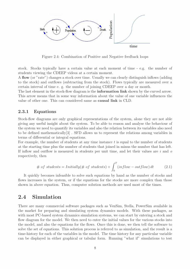
Figure 2.3: Negative feedback loop with delay� Combination of Positive and Negative Loops When positive and negative loops arecombined, a variety of patterns are possible. The example in fig 2.4 shows a situationwhere a positive feedback loop leads to early exponential growth, but then, after a delay,a negative feedback loop comes to dominate the behaviour of the system. This combi-nation results in an s-shaped pattern because the positive feedback loop leads to initialexponential growth, and then when the negative feedback loop takes over it leads to goalseeking behaviour.
2.3 Stock Flow Diagram (SFD)
As with a causal loop diagram, the stock-flow diagram shows relationships among variableswhich have the potential to change over time. The SFD consists of three different types ofelements: stocks, flows, and information. Unlike a causal loop diagram, a stock-flow diagramdistinguishes between different types of variables.A stock (or ”level variable”) is some entity that is accumulated over time by inflows and/ordepleted by outflows. Stocks can only be changed via flows. Mathematically a stock can beseen as an accumulation or integration of flows over time - with outflows subtracting from the
7
Figure 2.4: Combination of Positive and Negative feedback loops
stock. Stocks typically have a certain value at each moment of time - e.g. the number ofstudents viewing the CDEEP videos at a certain moment.A flow (or ”rate”) changes a stock over time. Usually we can clearly distinguish inflows (addingto the stock) and outflows (subtracting from the stock). Flows typically are measured over acertain interval of time e. g. the number of joining CDEEP over a day or month.The last element in the stock-flow diagram is the information link shown by the curved arrow.This arrow means that in some way information about the value of one variable influences thevalue of other one. This can considered same as causal link in CLD.
2.3.1 Equations
Stock-flow diagrams are only graphical representations of the system, alone they are not ablegiving any useful insight about the system. To be able to reason and analyse the behaviour ofthe system we need to quantify its variables and also the relation between its variables also needto be defined mathematically[3] . SFD allows us to represent the relations among variables interms of differential or integral equations.For example, the number of students at any time instance t is equal to the number of studentsat the starting time plus the number of students that joined in minus the number that has left.If inflow and outflow is measured in students per unit time, and let their values are i and orespectively, then
# of students = Initially(# of students) +
∫T
0
(inflow − outflow) dt (2.1)
It quickly becomes infeasible to solve such equations by hand as the number of stocks andflows increases in the system, or if the equations for the stocks are more complex than thoseshown in above equation. Thus, computer solution methods are used most of the times.
2.4 Simulation
There are many commercial software packages such as VenSim, Stella, PowerSim available inthe market for preparing and simulating system dynamics models. With these packages, aswith most PC-based system dynamics simulation systems, we can start by entering a stock andflow diagram for the model. We then need to enter the initial values for the various stocks intothe model, and also the equations for the flows. Once this is done, we then tell the software tosolve the set of equations. This solution process is referred to as simulation, and the result is atime-history for each of the variables in the model. The time history for any particular variablecan be displayed in either graphical or tabular form. Running ”what if” simulations to test
8
certain policies on such a model can greatly aid in understanding how the system changes overtime. System dynamics typically utilizes simulation to study the behaviour of systems and theimpact of alternative policies.We will be using the Vensim PLE simulation package[4] for CDEEP systems modeling, as it iseasy to use and it contains all the tools that we need for simulating and analysing our systemand most important factor is that it is available free of cost for educational purposes.
9
Chapter 3
Webcast Model
As discussed earlier, CDEEP System can be broadly classified into two sub-systems, the firstone involved in live transmission via EDUSAT, and the second doing live streaming of IITBCourses over the Internet (Webcast) started in January, 2008. Since both these sub-systemshave different set of viewers, and have different mode of transmission, we will consider bothas independent of each other and will be modeling them as two different systems. There arecurrently 4 studios from where lecture videos are recorded and transmitted over Internet atbandwidth of 100kbps per connection. To access these videos students need only a PC and aminimum 100kbps Internet connection.
3.1 Webcast system : Initial Model
To model the webcast system, we followed iterative approach, first we identified key variablesthat determine/change the behaviour of the system, and their dependencies through which theyaffect each other, for example Total available bandwidth and Quality of Video are two suchvariables, and increasing the bandwidth would result in improvement in the quality of videobecause more bandwidth per connection can be provided.Based on our understanding of the system, we identified important feedback loops in the system,as shown in the causal-loop diagram (fig. 3.1) and then we prepared equivalent Stock-flowdiagram (fig. 3.2) to model the system, where we distinguished variables among stock, flowand connectors. We simulated and analysed the system using Vensim simulator. Initially wefound following variables in system:
1. Total number of Students viewing the videos: This is the central variable in the system.This variable depends on student satisfaction, number of transmitted courses and qualityof videos.
2. Student satisfaction: This parameter is highly dependent on the quality of video beingtransmitted and number of courses being transmitted. To quantify this variable we as-sumed that it varies between 0 and 1, where 1 being the best possible and 0 being theworst.
3. Total number of courses being transmitted in a particular semester: This variable isconsidered as constant (=20) initially.
4. Server Performance: As the number of simultaneous connections increase processing loadon the server will also increase, and would result in server overloading and hence degra-
11
dation in quality of video. To quantify this variable we assumed that it varies between 0and 1, where 1 being the best possible and 0 being the worst.
5. Quality of video being transmitted: This variable consists of many parameters that de-termine the quality of video, such as jitter, audio-video sync, delay etc. To quantify thisvariable we assumed that it varies between 0 and 1, where 1 being the best possible (whentransmitted at 100kbps bandwidth) and 0 being the worst
6. Total available bandwidth: This is a constant and is taken as 8Mbps for our simulation.
7. Network bandwidth per connection: For each connection request to receive lecture videos100 kbps network bandwidth is provided until it exhausts whole 8Mbps capacity. Thatmeans that up to 80(= 8000/100) connections will get 100kbps bandwidth, and after thatwith for each incoming request this 8Mbps bandwidth will be equally divided among theviewer. Hence more the viewers less will be the bandwidth per connection, which willresult in poor quality of video at receiver end.
Using the above mentioned variables and their relations with one another we prepared aCasual Loop Diagram (CLD) (fig 3.2) and its corresponding Stock-flow Diagram(fig 3.3). Asit is simply visible in CLD that there are only two feedback loops in the system and since bothare negative feedback loops, as a result the system will show goal seeking or balancing kind ofbehaviour.
Figure 3.1: Causal Loop Diagram for Webcast system
We simulated this model in Vensim PLE simulator with initial values and equations shownin table 3.1.
12
Figure 3.2: Stock-flow Diagram for Webcast system
Table 3.1: Variables, values and, equations
VariableName
Initial Value/Equation/Range Unit
# of Student 100, Initial(# of students) +∫
T
0(inflow −
outflow) dtstudents
Inflow (Average student satisfaction∗Number of transmitted courses∗quality of video)
Bandwidth per connection/100), ranges be-tween 0 and 1
Dmnl (dimen-sionless)
Average studentsatisfaction
Quality of V ideo, ranges between 0 and 1 Dmnl
Number oftransmittedcourses
20 course
Number of Stu-dios
4 Dmnl (dimen-sionless)
13
Bandwidth perconnection
IF THEN ELSE(Total available bandwidth/Number of Students > 100, 100,T otal available bandwidth/Number of Students)
kbps/Student
Server Perfor-mance
IF THEN ELSE(# of students < 50001, (7000−Number of Students)/2000), ranges be-tween 0 and 1
Dmnl
3.1.1 Results and Discussion
We performed simulation runs for a time period of 4 years with varying values of differentvariables and obtained following results:
Figure 3.3: Change in Number of Students withtime
Figure 3.4: Quality of video with Bandwidthand server capacity
As it is visible in above graph that the variable Number of Students has become constant(=200 student) after 24 months, because the bandwidth per connections starts decreasing after80 connections (8Mbps/100kbps=80), and hence decreasing the quality of video which willeventually decrease the student satisfaction, this results in increase in outflow and decrease ininflow, that means more students leave the CDEEP and later on there becomes an equilibriumbetween inflow and outflow, hence no change in total number of students. To keep increasingnumber of students network bandwidth needs to be increased, as it is the only bottleneck in thesystem. As shown in fig. 3.4 the sever performance is constant (=1) throughout the simulation
14
period, because it is assumed that server can respond 5000 simultaneous requests before beingoverloaded, but this condition never arises because before reaching the limit of 5000 students,bandwidth becomes the bottleneck and hence students start leaving the courses.
If the total bandwidth is kept at infinite (let a very large value) even then also the numberof students will reach only 2000 because the number of courses becomes bottleneck and keepsinflow constant. If we consider an ideal case when available bandwidth is increased to infinite(meaning very high, say 10 Gbps) and number of courses is also increased from 20 to 80, eventhen also the number of students remain constant after 6667 as shown in fig 3.5, because serverstarts overloading after 5000 students and hence quality of video starts decreasing, which resultsin an increase in out flow.
Figure 3.5: Ideal case when bandwidth is infinite and courses transmitted is 80
3.1.2 Limitations
Current model has certain limitations such as it does not have any variable related to marketingof CDEEP program as it will have large impact on the rate at which new students join thesystem. Moreover current model didnt introduce any variable about the grants from MHRD andalso it considered the number of courses as a constant but in actual the number of transmittedcourses has increased almost linearly in each semester based on the feedback from students. Thenumber of transmitted course is also constrained be number of studios available for recordingthe lectures. It has been found that relevance of transmitted courses with other universitiesalso plays an important role, but was not considered in initial model.
3.2 Modified Webcast Model
After studying the system more closely and analysing the initial model, we found some morevariables that were not considered earlier, but they largely affect the behaviour of the system.
15
Following variables are included in the modified webcast model:
1. Grants form MHRD: Since CDEEP has received huge grants from MHRD after in April2009, this would be a key factor in dynamic behaviour of the system, as we can utilizethis money in various purposes. This event occurs only once. It is important to decidehow to distribute this money and what would be impact of it. The money can be utilizedin following manners:� Earlier as number of students increased the network bandwidth became bottleneck,
After getting grants CDEEP can outsource the network bandwidth, now an externalauthority will be responsible to serve thousands of students simultaneously with100kbps bandwidth for each student.� As the number of viewer increases demand for introducing more courses arrives.It is found that number of courses being transmitted is dependent on feedback ofviewers. To transmit more courses simultaneously more studios would be needed forrecording, number of studios can be increased from 4.� More money can be spent in marketing CDEEP programme, to increase the aware-ness about CDEEP among the potential students.� Currently CDEEP server is able to respond only 5000 requests simultaneously, afterthis it starts overloading. Money can be spent in upgrading the server.
2. Awareness about CDEEP videos: This is about, how more and more students are madeaware of and encouraged to join CDEEP program. To quantify this variable we assumedthat it varies between 0 and 1, where 1 being the best possible and 0 being the worst.
3. Number of studios: Currently there are 4 studios from where live courses are capturedand transmitted. If numbers of studio are increased then more courses can be transmittedsimultaneously. We assume that number of studios are increased from 4 to 6 after receivingthe grants.
4. Feedback from the students: Students give feedback about their experience of CDEEPlectures, for example about the video quality or if more courses need to be transmitted.This helps in improving the student satisfaction. To quantify this variable we assumedthat it varies between 0 and 1, where 1 being the best possible and 0 being the worst.
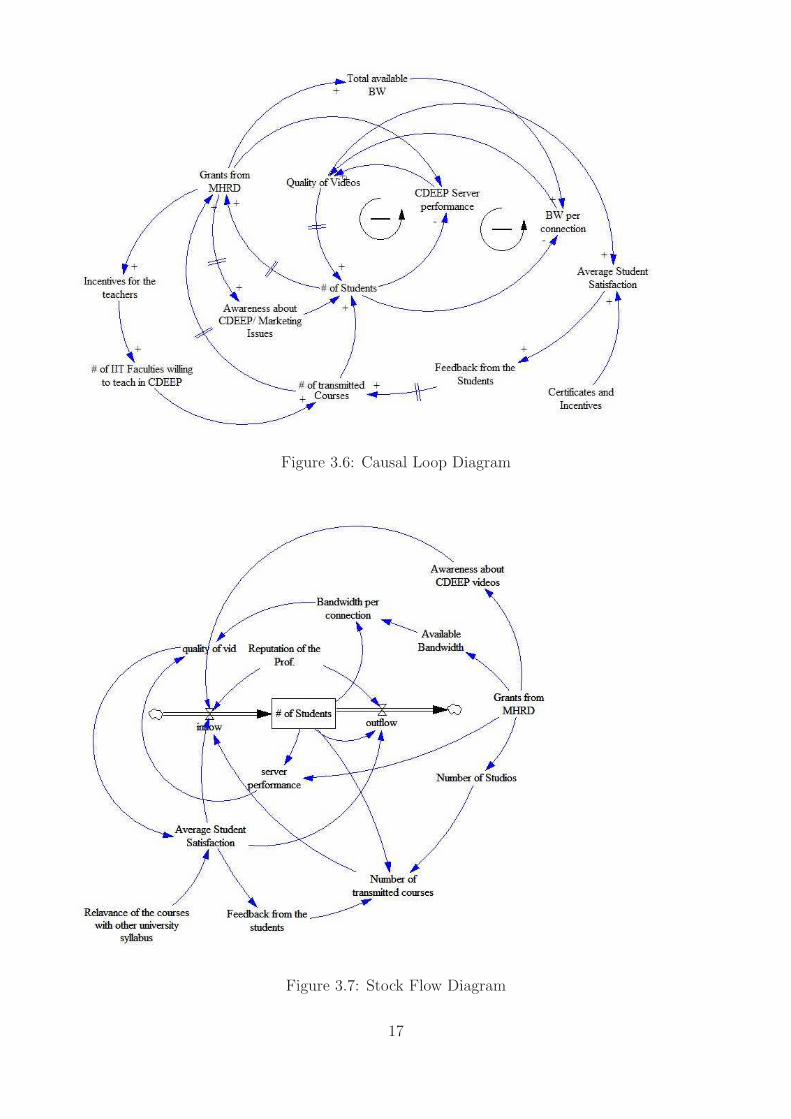
After including more variable we modified our previous Causal Loop Diagram (fig 3.6) andStock Flow Diagram(fig 3.7).
16
Figure 3.6: Causal Loop Diagram
Figure 3.7: Stock Flow Diagram
17
Table 3.2 shows major variables in the system as well as their initial values and equationsderived to show relation among different variables. These values were used for simulatingvarious scenarios which are discussed in next section.
Table 3.2: Variables, values and, equations
VariableName
Initial Value/Equation Unit
# of Student Initial(# of students)+∫
T
0(inflow−outflow) dt students
Inflow DELAY FIXED((”Reputation of the Prof.”∗Average Student Satisfaction∗Number of transmitted courses ∗ 10+Awareness about CDEEP videos ∗ 4), 2, 20)
studentsper month
Outflow INTEGER((1−Average Student Satisfaction)∗(1−”Reputation of the Prof.”)∗# of Students)
Studentsper month
Quality of videos Server performance ∗
Bandwidth per connection/100, ranges between0 and 1
Dmnl (dimen-sionless)
Grants fromMHRD
0, becomes 107̂ after 24 months Dmnl
Average studentsatisfaction
Quality of vid ∗ Relevance of the courseswith other university syllabus,ranges between 0and 1
Dmnl
Number oftransmittedcourses
IF THEN ELSE(Number of Studios > 5,INTEGER(20 + Feedback from the students∗”# of Students”/50),INTEGER(20 + Feedback from the students∗”# of Students”/35))
course
Number of Stu-dios
4, becomes 6 after 24 months Dmnl (dimen-sionless)
Total availablebandwidth
8000, becomes 107̂ after 24 months kbps
Bandwidth perconnection
Available Bandwidth/# of Students kbps
Server Perfor-mance
IF THEN ELSE(# of students < 50001, (7000− Number of Students)/2000)
dmnl
18
3.2.1 Results and Discussion
Figure 3.8: predicted number of students
Figure 3.9: Change in Server performance with number of students� Fig 3.8 shows predicted number of students for next 5 years, as it is visible number ofstudents becomes constant(=600) after 1 semester. but since after April 2009 (4 semesterafter starting the webcast program) huge money is invested in increasing bandwidth andnow the bandwidth becomes sufficient for all incoming students hence the quality ofvideo increases rapidly and reaches almost 1(highest possible) and student satisfactionalso increases the same way. As a result of this more and more students join CDEEP.After 45 months (4th semester after receiving grants) number of students stop increasingbeyond 5700 because server starts overloading as shown in fig 3.9 and starts dropping theconnections resulting in decrease in the quality of video. As a result of decrease in thequality of video students start leaving eventually, that decreases number of students andas a result again increases quality of video. This oscillation keep going on after that. Tokeep increasing the number of students, server performance should be improved after 22months after increasing the bandwidth.� After April 2009 if number of studios increases from 4 to 6, this will allow transmit-ting more courses simultaneously. Increase in the number of courses increases studentsatisfaction; it becomes another factor in increase in number of students.
19
3.2.2 Limitations� It was not always possible to quantify the relation between variables, for example howwill inflow change with Reputation of Professors, for such cases hit and try method wasthe only option. Many simulation runs needed to be performed with a different equationamong the variables.� Marketing issues could not be addressed because of lack of information and its effect onother events.� Actual information about number of students watching the IITB courses is available. itmakes it difficult to validate the model.� It is not possible in Vensim to use nested IF ELSE THEN while defining the relationamong the variables; hence we had to compromise from more realistic equations.
20
Chapter 4
EDUSAT Model
CDEEP transmits live courses through EDUSAT, ISRO’s satellite. These courses are trans-mitted unencrypted and anyone who has access to student interactive terminals (SITs) of theIndian Space Research Organization (ISRO) can freely tune in to these lectures and also inter-act live with IIT Bombay faculty. Those colleges who have installed SITs are known as RemoteCentres(RCs). Through the Student Interactive Terminals, two way live interaction is possiblebetween students at the RCs and the instructor at IITB. The courses are mainly intended forengineering college students and working professionals, hence the targeted audience is totallydifferent from those of live webcast.
4.1 Model Development
For modeling and analysing the functioning of EDUSAT system, we identified different variableswhich determine the behaviour of the system, by interacting and getting inputs from CDEEPstaff members. The key variables in the EDUSAT system are:� Number of Students: As discussed earlier, viewers of EDUSAT courses are college students
sitting at Remote Centres, and hence is totally different from the student variable ofwebcast model. As shown in Causal-loop diagram in fig 4.1 total number of studentsattending EDUSAT courses varies with other variables which are total number of remotecentres, number of transmitted courses, student satisfaction and quality of video receivedat remote centre.� Remote Centre coordinator: Coordinators are responsible for ensuring proper functioningat Remote Centre. If something goes wrong with reception of lectures at remote centre,they are the first to contact CDEEP staff. The incentives offered to the RC coordinatorsand their motivation are partly responsible for the number of IITB courses that thestudents in the RC choose to participate in. They also provide quick feedback regardingstudents’ interests in running courses.� Relevance of course: In interviews with Remote Centre (RC) coordinators and students,we found that the alignment of the transmitted IIT Bombay courses to the universitycurriculum was an important factor in determining whether students would continue toparticipate in CDEEPs courses. In India all universities have their own syllabus, still mostof the syllabus is common among them but syllabus of IITB courses is somewhat differentfrom other universities, and students at remote centres sometimes find EDUSAT coursesbeyond their syllabus. Therefore including this variable in our model is justifiable, as it
21
acts as an important factor in overall student satisfaction. While simulating, we quantifiedthis variable as a constant parameter whose value could be fixed as a number between0 and 1. In the Results section we discuss how the number of students depends on therelevance of the course.� Number of transmitted courses: CDEEP has been transmitting UG as well as PG coursefor various engineering streams. Number of courses transmitted through EDUSAT is notsame as webcast courses because out of four studios currently there is only one studiofrom where there is an up link for EDUSAT transmission. This variable also varies withthe feedback from students, whether they want CDEEP to introduce new courses are not.� Marketing efforts: This variable captures CDEEPs efforts at marketing its courses andto attract more and more institutes to become a remote centre. Through various meanssuch as newsletters, and workshops more number of institutes, and students are madeaware of CDEEP’s program. This variable has been quantified from a 0 to 1 scale in ourmodel.� Support staff for equipment maintenance: They play an important role in proper func-tioning at remote centres. Many times it happens that even after getting complainsabout bed equipment conditions, immediate maintenance can not be done due to lack ofsufficient support staffs.
Some variables are common between the webcast and EDUSAT model. Yet, the samevariable is part of different feedback loops in the two models. One such example is:� Quality of videos. In the Webcast model, the video quality of the course that a student
participates in mainly depends on the availability of sufficient bandwidth, which changeswith number of simultaneous connections. While EDUSAT have a dedicated 1 Mbps uplink and 500 kbps down link for transmission. In the EDUSAT model, the video qualityis affected by the condition of the Equipment at the RC. This variable has again beenquantified on a scale of 0 to 1, and it has been held at a constant value of 0.5 whichrepresents the average condition of equipment at the RCs.
Using these variables and their interaction with one-another we have prepared the CausalLoop diagram for the model in fig. 4.1. This diagram shows how different feedback loops inthe systems that are responsible for its non-linear behaviour. Using this diagram we prepareda corresponding Stock-flow diagram (shown in fig. 4.2) in Vensim simulator.
22
Figure 4.1: Causal Loop Diagram
Figure 4.2: Stock Flow Diagram
For simulation of the above model, values of different variables were gathered from theCDEEP staff. We also derived some equations which represent the relation among the vari-ables. Table 4.1 shows different variables, their corresponding initial values or the equation todetermine the variable and the units of all the variables in model.
23
Table 4.1: Variables, values and, equations for initial model
Variable Name Initial Value/Equation Unit
# of Student Initial(# of students)+∫
T
0(inflow−outflow) dt students
Inflow DELAY FIXED((”Reputation of the Prof.”∗Average Student Satisfaction∗Number of transmitted courses ∗ 10+Awareness about CDEEP videos ∗ 4), 2, 20)
studentsper month
Outflow INTEGER((1−Average Student Satisfaction)∗(1−”Reputation of the Prof.”)∗# of Students)
Studentsper month
Relevance withother univ. syl-labus
0.6 dmnl
Quality of videos Equipment condition at RC Dmnl (dimen-sionless)
Grants fromMHRD
0, becomes 107̂ after 24 months Dmnl
Average studentsatisfaction
Quality of vid ∗ Relevance of the courseswith other university syllabus
Dmnl
Number oftransmittedcourses
IF THEN ELSE(Number of Studios > 5,INTEGER(20 + Feedback from the students∗”# of Students”/50),INTEGER(20 + Feedback from the students∗”# of Students”/35))
course
Number of Stu-dios
1 Dmnl (dimen-sionless)
4.2 Results and Discussion
We performed simulation runs of EDUSAT model for different scenarios, and analysed theresults. We considered following scenarios:
1. Behaviour of existing system and effect of incoming grants: In figure 4.3 we have shownthe future behaviour of the system as well as the the effect of incoming grants. If theCDEEP system runs in its regular annual budget and no extra grants enter the system,then the maximum number of students is about 600 even after a period of 5 years, whichis very less than what is the goal of CDEEP. Since CDEEP has received huge one-timegrants from MHRD, If we include this grant entering the system at month 24, then thenumber of students increases to 2400 after 5 years. In the simulation the grants have beenused to increase the number of studios from 1 to 4 and also marketing expenses have beenincreased to 0.7 from 0.3.
2. Marketing vs Number of courses: Instead of concentrating on only marketing aboutCDEEP, we need to concentrate on increasing the number of courses transmitted persemester as well. According to the simulation results if we are putting efforts in marketingonly, we can increase the number of students up to 315 after 18 months. And if we increasethe number of courses 45 without concentrating on marketing then we would fetch at most
24
Figure 4.3: Effect of Incoming Grants
Figure 4.4: increase in number of students withnumber of transmitted courses
Figure 4.5: increase in number of students withmarketing expenses
260 to 270 students after 18 months, but If we increment the number of courses to 20and put some efforts in marketing too ( 0.7 out of 1) we get significant improvement innumber of students and it reaches to 373 after 18 months.
3. Relevance of the courses with other universities: As mentioned in section 4.1, the align-ment of the syllabus of IIT Bombays transmitted courses to the curriculum followed bythe students in the RCs is of great significance. In Figure 4.6, we see the how the courserelevance affects the number of students. If a course has low relevance, say 0.2 on a scaleof 0 to 1, then the number of students in fact decreases from 6 to 12 to 18 months. whileIf a course has high relevance, say 0.8, then the number of students increases. Further,the increase or decrease of students occurs at a faster rate at the 18 months than at 6months. This shows that the impact of course relevance becomes even stronger as moretime goes by.
25
Figure 4.6: Effect of relevance of courses
A poster titled ”Using System Dynamics to Model and Analyse a Distance Edu-cation Program”, covering our model and the results obtained through the simulations, hasbeen accepted in International Conference on Information and Communication Technologiesand Development 2010.
4.3 Recommendations
The results from the system dynamics simulation of EDUSAT model along with results fromWebcast model gave us valuable insights into making policy decisions in our program. Atfirst significant improvement in network bandwidth is needed, as it is the first resource whichbecomes bottleneck(fig 3.4), because of this quality of videos degrades and as a result number ofstudents stop increasing after a certain limit. Investment made in purchasing more bandwidthwill result in very rapid increase in number of students (fig 3.8). Another recommendationthat emerges from our study is that sufficient attention should be paid for obtaining highquality servers but it is needed only few months after bandwidth is increased, because serverperformance would become a bottleneck later on (fig 3.9). In addition attention needs to bepaid on publicizing CDEEP programs and encouraging student to join CDEEP (fig 4.5).
We studied the role injection of grants into the system. Even though this was a one-timeevent, its effect is significant. Even if CDEEP administrators seek extra funding for the systemonly once in while, it will help in improving the outreach of its courses, provided the fundsare distributed in an optimal manner to various parts of the system. The system dynamicsmodeling tool has proved to be very useful in this case as a predictive mechanism. The distanceeducation programs administrators could use the simulation results to determine what partsof the program should be allocated what percentage of funds, and at which times. If CDEEPwants to achieve its goal of reaching out to a large number of students, it is essential that thecourses transmitted by CDEEP are well aligned with the specific curricula of students who areviewing the courses (fig 4.6).
26
Chapter 5
System Dynamics Modeling Tools
Having performed the modeling and simulations of CDEEP system model, we took studyingsystem dynamics modeling tools as our next task, and see if we could contribute for the de-velopment of system dynamics simulators. In our study we found that the System Dynamicsmodeling methodology is a 50 year old technique but still there is no standardization of model-ing framework. The current software tools are proprietary applications. There is generally verylimited collaboration among them. Opensource solutions available at Sourceforge[5] includeSphinx, OpenSim, SystemDynamics and SystemML. These projects have failed to be com-pleted by developers or utilized by researchers and consultants because their underlying datastructures (their information models) were inadequately defined. These solutions all implementincompatible or incomplete information models except for elements of a few of the most basicmodel components. Hence no truly successful open source System Dynamics model builder orsimulation applications is currently available.
We explored SystemDynamics [6], an open source system dynamics modeling tool availableat Sourceforge, aiming to make contribution to the open source community via adding somenew features or fix any bug in software, but there was no proper documentation of the codeavailable, and the code was too huge(around 50K lines of code) to be understood withoutdocumentation. Hence we dropped the idea modifying the software, but while exploring thecode we identified major components of a system dynamics simulation model. We also referredthe System Dynamics Information Model project[7] that had taken an initiative to prepare amodern framework about system dynamics models, and prepared a higher level flowchart (figure5.1) of system dynamics information model framework and shown various model objects (suchas stocks and flows), the scope of their relationships, and the necessary operations performedduring model building and simulation.
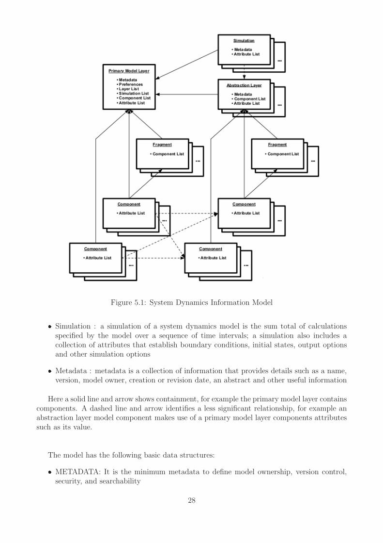
In figure 5.1, the following elements are introduced:� Component: a model component is a basic system dynamics function block such as astock or flow.� Fragment: a fragment is a collection of model components i. e. it is a subset of the model� Primary Model Layer: the primary model layer represents the fundamental model, thisfundamental model can be the entire model, or it may be core part of the model to whichother parts of the model may refer for internal variable values� Abstraction Layer : an abstraction layer is a separate layer of the model that facilitatesmodel partitioning, and simulation partitioning; an abstraction layer refers to the primarymodel layer for interval variable values
27
Figure 5.1: System Dynamics Information Model� Simulation : a simulation of a system dynamics model is the sum total of calculationsspecified by the model over a sequence of time intervals; a simulation also includes acollection of attributes that establish boundary conditions, initial states, output optionsand other simulation options� Metadata : metadata is a collection of information that provides details such as a name,version, model owner, creation or revision date, an abstract and other useful information
Here a solid line and arrow shows containment, for example the primary model layer containscomponents. A dashed line and arrow identifies a less significant relationship, for example anabstraction layer model component makes use of a primary model layer components attributessuch as its value.
The model has the following basic data structures:� METADATA: It is the minimum metadata to define model ownership, version control,security, and searchability
28
� PREFERENCES: These are a set of settings that affects appearance, abstraction andother model-specific qualities such as symbol size, symbol spacing� COMPONENT LIST: The unique set of registered names of model components andfragments contained in the model primary layer for example component name, type,shape, location etc.� LAYER LIST: It defines a list of abstraction layers in the model� SIMULATION LIST: It contains the list of named simulation scenarios.
Here a system dynamics model has been described in the form of information model withits data structures. An open source information model specification is the first step for anyfurther specification work or application development. Follow-on open source projects mayinclude an open source metadata specification that is compatible with another open sourceprojects to enable model warehousing. The primary benefit of the specification will be improvedcollaboration between researchers who currently use various proprietary tools for their work.A formal specification of the methodology will also improve the communication of ideas, andthe proprietary tool vendors may be convinced to include open source model import / exportmethods into their products.
29
Chapter 6
Conclusion and Future Work
In this project we modeled CDEEP program from a systems behaviour perspective. Byanalyzing the structure of CDEEP using system dynamics simulations, we obtained insightsinto performance of the program. Many of these results could not have been obtained bysimply looking at isolated events and their consequences, due to the various interacting partswithin the system. Results from the simulations gave us understanding about possible factorsto improve the behaviour of the system. We might not have considered some of these factorsin CDEEP future plans without this study.
It would be worthwhile for institutions that are starting a distance education program toanalyze their plan using a systems dynamics model. Early warnings of the possible pitfallsin the plan could emerge from the results of the simulations. New aspects that had not beenanticipated could become visible. Distance education programs that are already functionalwould also benefit from running a system dynamics simulation of their program. Due to thecomplex nature of systems behaviour, results of a system dynamics simulation are often notobvious. These results prove to be useful for existing problems, making policy changes andstrategic decisions. Program administrators could get an insight into questions such as: whatwould happen if a certain policy were changed, or how would we distribute existing resourcesinto different parts of the system. System dynamics offers us a theoretical tool to analyze sucha structure, and gain an understanding into the performance of the system.
As continuation of this work, results and recommendations made could be validated by imple-menting them over the actual CDEEP system. The Webcast and EDUSAT models have beenprepared after getting inputs from CDEEP staffs, past data and the feedback gathered fromstudents, and hence the results are as good as the model itself Since we could not implementour policy recommendations on the CDEEP, and see the validity of our claims. This task canbe done in the subsequent work.The current software tools for system dynamics modeling are proprietary applications. Open-source projects for such tools have failed to be completed by developers or utilized by researchersand consultants because their underlying information model were inadequately defined. Notruly successful open source System Dynamics model builder or simulation tools are currentlyavailable. This task can be taken in hand to improve the tools, and to expand the applicationof this modeling technique to a broader community of users.
[8] System Dynamics Modelling, A Practical Approach. Chapman & Hall, 1996.
[9] McKansey Global Institute. Emerging global labour market. 2005.
[10] Deepak B. Phatak Kannan M. Moudgalya and R. K. Shevgaonkar. Engineering educationfor everyone: A distance education experiment at iit bombay. Frontiers in Education,2008.