Approximate structural optimization using kriging method and digital modeling technique considering noise in sampling data Sei-Ichiro Sakata a, * , Fumihiro Ashida a , Masaru Zako b a Department of Electronic Control Systems Engineering, Interdisciplinary Faculty of Science and Engineering, Shimane University, 1060 Nishikawatsu-cho, Matsue, Shimane, Japan b Department of Management of Industry and Technology, Graduate School of Engineering, Osaka University, 2-1 Yamada-Oka, Suita, Osaka, Japan Received 5 March 2007; accepted 30 April 2007 Available online 18 June 2007 Abstract This paper describes a combination approach of a digital finite element modeling technique and the Kriging method for structural optimization. Since the digital modeling technique includes some inaccuracies in a modeling process, applicability of the Kriging method to noisy data is investigated. An estimated surface generated by the conventional Kriging method will be wavy and not appropriate to approximate optimization with noisy data. Therefore, a new Kriging-based approach is proposed. The new class of the Kriging method and a digital modeling technique is applied to an eigenfrequency optimization of a structure. Numerical examples illustrate a validity and effectiveness of the proposed method. Ó 2007 Elsevier Ltd. All rights reserved. Keywords: Approximate optimization; Structural optimization; Noisy data; Digital finite element model; Kriging method; FEM 1. Introduction In this paper, a combination approach of an approxi- mate optimization method and a digital modeling tech- nique for approximate structural optimization is discussed. A digital modeling technique will reduce a mod- eling cost, however, an object function can be evaluated discretely. Therefore, approximate optimization method will be available for structural optimization using a digital modeling technique. Several approximate optimization methods will be effec- tive for an engineering optimization. In addition to conven- tional methods using polynomial-based approximation [1], spline interpolation [2], neural network (NN) [3], radial basis function method (RBF) [2] or Kriging method [4,5] has been recently studied for an approximate optimization. Especially, NN, RBF or Kriging method is applicable to generate an approximated surface of a non-linear and com- plex unknown function because of its flexibility. On the other hand, those methods may not be suitable to generate an estimated response surface with using noisy data, since those methods will generate an approximated response surface to minimize approximation errors at a sampling location. For example, an estimated surface by the conven- tional Kriging method will be complete interpolation of sampling data [6]. This fact means that those methods will regard noisy data as exact data, therefore the approxi- mated surface will faithfully include noises in sampling results. In some cases as optimization with noisy data caused by modeling errors or numerical errors or experi- mental data, those methods should be carefully used for approximation. Some conventional methods, such as a polynomial-based approximation method, will be more applicable in those cases, however it will be difficult to assume an appropriate base function, especially in the case of highly non-linear, high dimensional and unknown response function. 0045-7949/$ - see front matter Ó 2007 Elsevier Ltd. All rights reserved. doi:10.1016/j.compstruc.2007.05.007 * Corresponding author. Tel./fax: +81 852 32 6840. E-mail addresses: [email protected](S.-I. Sakata), ashida@ ecs.shimane-u.ac.jp (F. Ashida), [email protected](M. Zako). www.elsevier.com/locate/compstruc Available online at www.sciencedirect.com Computers and Structures 86 (2008) 1477–1485
Transcript
Available online at www.sciencedirect.com
www.elsevier.com/locate/compstruc
Computers and Structures 86 (2008) 1477–1485
Approximate structural optimization using kriging method anddigital modeling technique considering noise in sampling data
Sei-Ichiro Sakata a,*, Fumihiro Ashida a, Masaru Zako b
a Department of Electronic Control Systems Engineering, Interdisciplinary Faculty of Science and Engineering, Shimane University,
1060 Nishikawatsu-cho, Matsue, Shimane, Japanb Department of Management of Industry and Technology, Graduate School of Engineering, Osaka University, 2-1 Yamada-Oka, Suita, Osaka, Japan
Received 5 March 2007; accepted 30 April 2007Available online 18 June 2007
Abstract
This paper describes a combination approach of a digital finite element modeling technique and the Kriging method for structuraloptimization. Since the digital modeling technique includes some inaccuracies in a modeling process, applicability of the Kriging methodto noisy data is investigated. An estimated surface generated by the conventional Kriging method will be wavy and not appropriate toapproximate optimization with noisy data. Therefore, a new Kriging-based approach is proposed. The new class of the Kriging methodand a digital modeling technique is applied to an eigenfrequency optimization of a structure. Numerical examples illustrate a validity andeffectiveness of the proposed method.� 2007 Elsevier Ltd. All rights reserved.
Keywords: Approximate optimization; Structural optimization; Noisy data; Digital finite element model; Kriging method; FEM
1. Introduction
In this paper, a combination approach of an approxi-mate optimization method and a digital modeling tech-nique for approximate structural optimization isdiscussed. A digital modeling technique will reduce a mod-eling cost, however, an object function can be evaluateddiscretely. Therefore, approximate optimization methodwill be available for structural optimization using a digitalmodeling technique.
Several approximate optimization methods will be effec-tive for an engineering optimization. In addition to conven-tional methods using polynomial-based approximation [1],spline interpolation [2], neural network (NN) [3], radialbasis function method (RBF) [2] or Kriging method [4,5]has been recently studied for an approximate optimization.
0045-7949/$ - see front matter � 2007 Elsevier Ltd. All rights reserved.
Especially, NN, RBF or Kriging method is applicable togenerate an approximated surface of a non-linear and com-plex unknown function because of its flexibility. On theother hand, those methods may not be suitable to generatean estimated response surface with using noisy data, sincethose methods will generate an approximated responsesurface to minimize approximation errors at a samplinglocation. For example, an estimated surface by the conven-tional Kriging method will be complete interpolation ofsampling data [6]. This fact means that those methods willregard noisy data as exact data, therefore the approxi-mated surface will faithfully include noises in samplingresults. In some cases as optimization with noisy datacaused by modeling errors or numerical errors or experi-mental data, those methods should be carefully used forapproximation. Some conventional methods, such as apolynomial-based approximation method, will be moreapplicable in those cases, however it will be difficult toassume an appropriate base function, especially in the caseof highly non-linear, high dimensional and unknownresponse function.
Fig. 2. Same digital model expressing two different smooth shapes.
1478 S.-I. Sakata et al. / Computers and Structures 86 (2008) 1477–1485
Therefore, in this paper, the Kriging method isimproved to be applied to estimate a response surface withusing noisy data. By comparing both estimated results ofthe proposed and conventional Kriging method, at first,effectiveness of the proposed Kriging method is discussed.We propose a combinatorial use of a digital finite modelingtechnique and the proposed Kriging method for an approx-imate structural optimization problem. By a numericalresult of shape optimization problem solved by using botha digital finite element modeling and the Kriging method,applicability and effectiveness of the proposed method isinvestigated.
2. Approximate shape optimization using digital finiteelement model
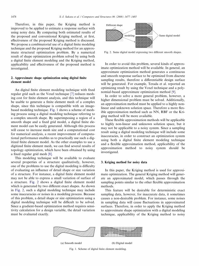
An digital finite element modeling technique with fixedregular grid such as the Voxel technique [7] reduces mesh-ing cost for finite element analysis, and this technique willbe usable to generate a finite element mesh of a complexshape, since this technique is compatible with an image-based modeling technique. Fig. 1 shows a scheme of mesh-ing process using a digital modeling technique referring toa complex smooth shape. By superimposing a region of asmooth shape and a fixed grid model, a digital finite ele-ment model can be easily generated. Although this processwill cause to increase mesh size and a computational costfor numerical analysis, a recent improvement of computa-tional performance enables us to practically use such a dig-itized finite element model. As the other examples to use adigitized finite element mesh, we can find several results oftopology optimization, which have been obtained by usinga fixed regular grid mesh [8].
This modeling technique will be available to evaluateseveral properties of a structure qualitatively, however,one of the problems to use the digital modeling is difficultyof evaluating an influence of detail shape or size variationof a structure. For instance, a digital finite element modelmay not be able to express a small variation of surface ofa structure. Fig. 2 shows a digital finite element modelwhich is generated by two different exact shapes. As shownin Fig. 2, such a digital modeling technique may includesome inaccuracies or noises in a modeling process. Becauseof this problem, a detail shape or size optimization using adigital modeling technique will be difficult to be solved.Since a gradient-based optimization method requires sensi-tivity calculation for a design variable, the detail variationmust be evaluated exactly.
(a) Smooth model
Fig. 1. Scheme of digital fi
In order to avoid this problem, several kinds of approx-imate optimization method will be available. In general, anapproximate optimization method generates a continuousand smooth response surface to be optimized from discretesampling results, therefore a differentiable design surfacewill be generated. For example, Terada et al. reported anoptimizing result by using the Voxel technique and a poly-nomial-based approximate optimization method [9].
In order to solve a more general problem, however, ahigher dimensional problem must be solved. Additionally,an approximation method must be applied to a highly non-linear and unknown solution space. Therefore a more flex-ible approximation method such as NN, RBF or the Kri-ging method will be more available.
These flexible approximation methods will be applicableto highly non-linear and unknown solution space, but itmay not be applicable to a noisy system. Since a samplingresult using a digital modeling technique will include someinaccuracies, in order to construct an optimization systemusing both a digital finite element modeling techniqueand a flexible approximation method, applicability of theapproximation method to noisy system should beinvestigated.
3. Kriging method for noisy data
In this paper, the Kriging method is used for approxi-mate optimization. The general Kriging method will gener-ate an approximated model, which passes through thesampling points similar to the other flexible approximationmethods.
This feature will be desirable for deterministic exactsampling data, however, for inaccurate data, it sometimescauses a non-desirable problem. For instance, some noisesin sampling data will cause fluctuations in approximatedsurfaces. Therefore, in order to apply the Kriging methodto approximate shape optimization with a digital modelingtechnique, applicability of the Kriging method to noisy
(b) Digital model
nite element modeling.
S.-I. Sakata et al. / Computers and Structures 86 (2008) 1477–1485 1479
data should be investigated, because a digital modelingtechnique will include some inaccuracies in modelingprocess.
Several types of the Kriging system have been proposed.The maximum likelihood estimator (MLE)-based Krigingsystem, which was reported by Sacks et al. [4], is generallyused for an approximate optimization. However, the ordin-ary Kriging method with an empirical semivariogram-based parameter estimation is used in this study. Theordinary Kriging method provides an estimate valuebZðs0Þ at a location s0 as
bZðs0Þ ¼ wT Z ð1Þ
where w = {w1,w2, . . . ,wn}T is a weighting coefficient vectorfor linear prediction (Eq. (1)), Z = {Z(s1), . . . ,Z(sn)}T is ob-served values as sampling results at sampling locations1 . . . sn.
To determine w, we will optimize a set of semivariogramparameter to minimize a mean estimation error. Using asemivariogram function c, Eq. (1) can be rewritten as
bZðs0Þ ¼ C�1c� þ 1� 1T C�1c�
1T C�11
� �C�11
� �T
Z ð2Þ
where Cij = c(si � sj), c�i ¼ c�ðsi � s0Þ and 1 = {1,1, . . . , 1}T.In this study, the following Gaussian-type semivariogramfunction is used.
cðhi; bÞ ¼b0 þ b1 1� exp � hij j
b2
n o2� �� �
hij j 6¼ 0
0 hij j ¼ 0
8<: ð3Þ
where b = {b0,b1,b2} is a set of semivariogram parameters.In the conventional method, c* will have the same form asEq. (3). Therefore, the ordinary Kriging method gives asame estimated value as the sampling value at samplinglocation. b0 in Eq. (3) indicates the nugget effect, and thisterm causes discontinuity in an estimated surface [6]. Ifb0 is not considered, the estimated surface will smoothlyinterpolate given data, but this fact will cause to generatea noise-included estimated surface. In the Kriging system,therefore, the nugget effect should be considered, especiallyin the case of using noisy data.
On the other hand, to eliminate discontinuity of an esti-mate surface, a semivariogram function for an estimatedvalue is improved. Because of an assumption of second-order stationarity of sampling space, the conditionc(0) = 0 must be satisfied, but this restriction is removedin an estimated surface. Namely, we assume
c�ðhi; bÞ ¼ b0 þ b1 1� exp � hij jb2
� �2 !" #
ð4Þ
Since it is considered that discontinuity of an estimated sur-face is caused by that of semivariogram function for anestimated surface, using Eq. (4) will enable to eliminate dis-continuity of an estimated surface.
4. Improved empirical semivariogram for noisy data
To determine a set of semivariogram parameters, we canuse an empirical semivariogram. Cressie proposed a robustefficient estimator for changes in the scale of data using thistype of semivariogram [10]. An empirical semivariogrammodel used for determination of a set of semivariogramparameters can be expressed as
cðhÞ ¼ 1
2jNkjXNk
ðZðsiÞ � ZðsjÞÞ2 ð5Þ
where Nk is a set of data, which satisfy jsi � sjj 2 ðRk�1;Rk�; 0 < Rk�1 < Rk 2 R1. Rk is an optional real constantto classify a set of sampling data. In general, Z(si) will bean exact observed value. If Z(si) includes some noises e, how-ever, jZ(si) � Z(sj)j will include an estimation error of 2e orless. Since the nugget effect b0 can be interpreted as an aver-age jump value from an exact surface, it can be assumed asjej = jb0j in an average meaning. Assuming a degree of dis-persion of data equal to a twice of an average nugget effectb0, the empirical semivariogram Eq. (5) can be expressed as
c�ðhÞ ¼ cðhÞ � 8b20 ð6Þ
Eq. (6) is used in minimizing the Cressie’s criterion insteadof cðhÞ itself. Since Eq. (5) will be non-linear on b0, someeffective algorithms such as Brunell’s approach [11] cannotbe used. Therefore, in this study, a conventional non-linearoptimization procedure is used for the minimizing process.
In this paper, the Kriging method using Eqs. (3), (4) and(6) is proposed, and it is applied to a digital finite elementmodeling process based structural optimization. Thisimprovement and the smoothed Kriging using Eq. (4) arethe key idea of the proposed new class of the Krigingmethod.
5. Investigation of applicability of the Kriging method to
noisy data
In order to investigate applicability and effectiveness ofthe proposed method to estimation of a response surfacewith noisy data, at first, a one-dimensional mathematicalfunction is estimated. In this case, the following functionis used as the exact function.
f ðxÞ ¼ �x sinð2xÞ þ 0:2xþ 1; 0 6 x 6 5 ð7Þ
At first, estimated results by the proposed method in thecase of a noiseless problem are compared with that of theconventional approach.
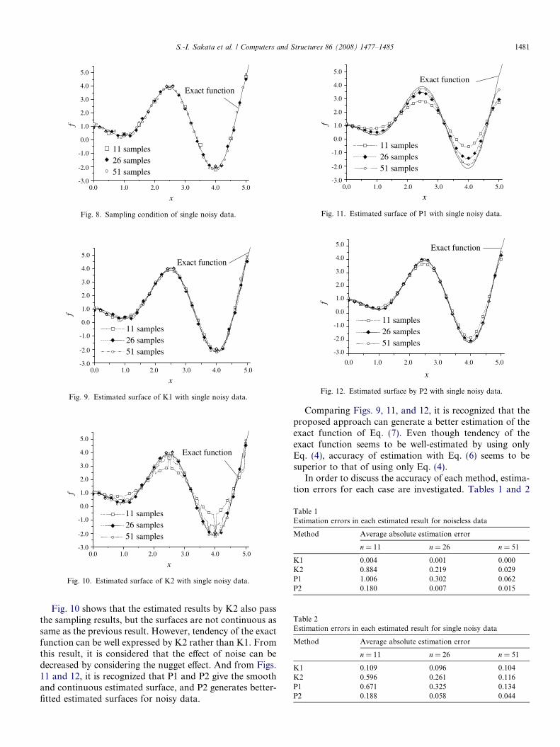
In this case, n = 11, 26 and 51 sampling results are usedfor estimation. n shows the number of sampling locations(grids). Fig. 3 shows a sampling condition for noiselessdata. The solid line in figures shows an exact curve ofEq. (7). Fig. 4 shows the estimated results by using the con-ventional ordinary Kriging system without considering thenugget effect (K1). Fig. 5 shows the results of using the con-ventional ordinary Kriging system with considering the
Exact function
-3.0
-2.0
-1.0
0.0
1.0
2.0
3.0
4.0
5.0
f
0.0 1.0 2.0 3.0 4.0 5.0
x
11 samples 26 samples51 samples
Fig. 3. Sampling condition of noiseless data.
Exact function
-3.0
-2.0
-1.0
0.0
1.0
2.0
3.0
4.0
5.0
f
0.0 1.0 2.0 3.0 4.0 5.0
x
11 samples 26 samples51 samples
Fig. 4. Estimated surface of K1 with noiseless data.
Exact function
-3.0
-2.0
-1.0
0.0
1.0
2.0
3.0
4.0
5.0
f
0.0 1.0 2.0 3.0 4.0 5.0
x
11 samples 26 samples51 samples
Fig. 5. Estimated surface of K2 with noiseless data.
Exact function
-3.0
-2.0
-1.0
0.0
1.0
2.0
3.0
4.0
5.0
f
0.0 1.0 2.0 3.0 4.0 5.0
x
11 samples 26 samples51 samples
Fig. 6. Estimated surface of P1 with noiseless data.
Exact function
-3.0
-2.0
-1.0
0.0
1.0
2.0
3.0
4.0
5.0
f
0.0 1.0 2.0 3.0 4.0 5.0
x
11 samples 26 samples51 samples
Fig. 7. Estimated surface of P2 with noiseless data.
1480 S.-I. Sakata et al. / Computers and Structures 86 (2008) 1477–1485
nugget effect (K2), Fig. 6 shows the result of using only Eq.(4) (P1), and Fig. 7 shows estimated results by using theproposed method using Eqs. (4) and (6) (P2).
From Fig. 4, it is recognized that the conventionalmethod without considering the nugget effect gives verysmooth and appropriate estimation. From Fig. 5, it isfound that the conventional method with considering thenugget effect generates a discontinuous surface, and theestimation errors in function values tend to be larger asthe sampling number decreases. This tendency can be also
found in the case of using P1, but it is recognized fromFig. 6 that the estimated surface of P1 is continuous andsmooth.
Fig. 7 shows the estimated surface by the proposedmethod. It is recognized that the estimated surface is con-tinuous, and includes less errors than that of K2 or P1,especially in the case of a small number of sampling data.
As a next example, the Kriging systems are applied toanother set of sampling data with random noise. It is con-sidered the case that there is single data for each grid. Thesampling results with random noises are computed by
�f ðxÞ ¼ f ðxÞ þ ð�1ÞP �max f ðxÞ � p � ef ð8Þwhere 0 6 p 6 1 is a random value and ef is a small realconstant. We assume ef = 0.05 in this case.
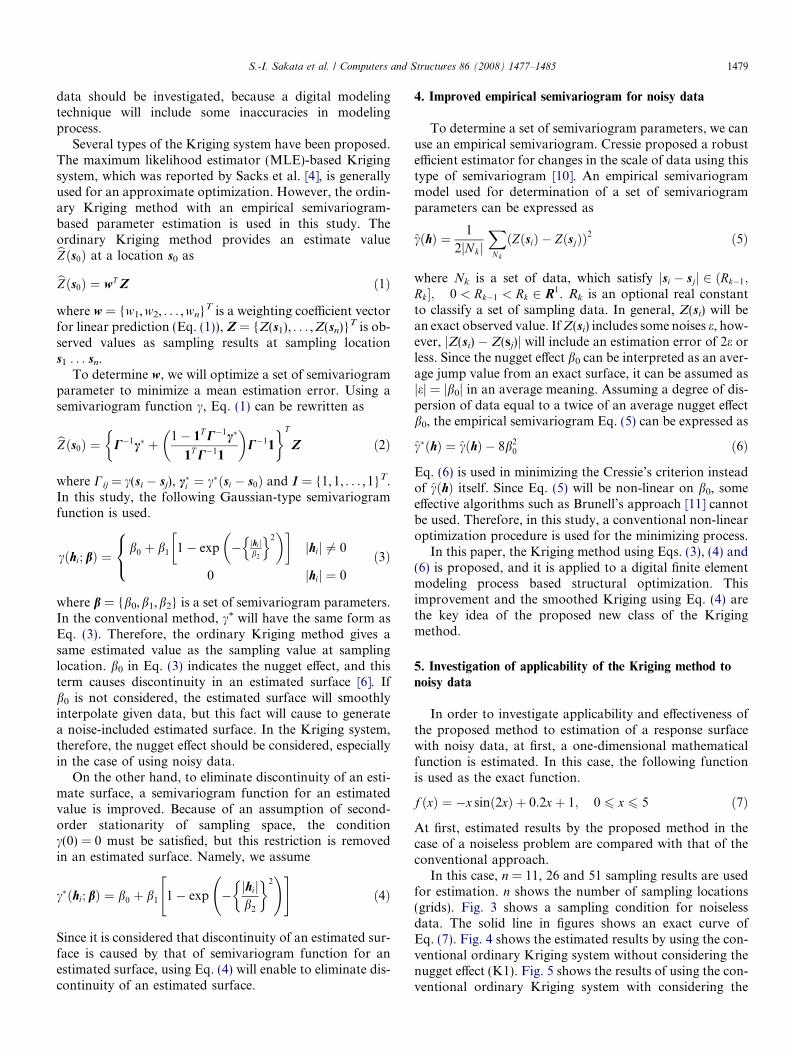
Fig. 8 shows the sampling condition. From Fig. 8, it canbe recognized that some noises are included in the samplingresults. Figs. 9–12 show the estimated results of K1, K2, P1and P2. From Figs. 8 and 9, the estimated surfaces by K1are continuous and smooth, and pass through the samplingresults. This result shows that K1 gives a complete interpo-lation even if some noises are included in sampling results.The estimated surfaces by K1 are locally wavy, and it isconsidered that K1 will not applicable to approximate opti-mization with noisy data.
Exact function
-3.0
-2.0
-1.0
0.0
1.0
2.0
3.0
4.0
5.0
f
0.0 1.0 2.0 3.0 4.0 5.0
x
11 samples 26 samples51 samples
Fig. 10. Estimated surface of K2 with single noisy data.
Exact function
-3.0
-2.0
-1.0
0.0
1.0
2.0
3.0
4.0
5.0
f
0.0 1.0 2.0 3.0 4.0 5.0
x
11 samples 26 samples51 samples
Fig. 11. Estimated surface of P1 with single noisy data.
0.0 1.0 2.0 3.0 4.0 5.0
-3.0
-2.0
-1.0
0.0
1.0
2.0
3.0
4.0
5.0 Exact function
f
x
11 samples 26 samples 51 samples
Fig. 12. Estimated surface by P2 with single noisy data.
Exact function
-3.0
-2.0
-1.0
0.0
1.0
2.0
3.0
4.0
5.0f
0.0 1.0 2.0 3.0 4.0 5.0
x
11 samples 26 samples51 samples
Fig. 8. Sampling condition of single noisy data.
Exact function
-3.0
-2.0
-1.0
0.0
1.0
2.0
3.0
4.0
5.0
f
0.0 1.0 2.0 3.0 4.0 5.0
x
11 samples 26 samples51 samples
Fig. 9. Estimated surface of K1 with single noisy data.
Table 1Estimation errors in each estimated result for noiseless data
S.-I. Sakata et al. / Computers and Structures 86 (2008) 1477–1485 1481
Fig. 10 shows that the estimated results by K2 also passthe sampling results, but the surfaces are not continuous assame as the previous result. However, tendency of the exactfunction can be well expressed by K2 rather than K1. Fromthis result, it is considered that the effect of noise can bedecreased by considering the nugget effect. And from Figs.11 and 12, it is recognized that P1 and P2 give the smoothand continuous estimated surface, and P2 generates better-fitted estimated surfaces for noisy data.
Comparing Figs. 9, 11, and 12, it is recognized that theproposed approach can generate a better estimation of theexact function of Eq. (7). Even though tendency of theexact function seems to be well-estimated by using onlyEq. (4), accuracy of estimation with Eq. (6) seems to besuperior to that of using only Eq. (4).
In order to discuss the accuracy of each method, estima-tion errors for each case are investigated. Tables 1 and 2
1482 S.-I. Sakata et al. / Computers and Structures 86 (2008) 1477–1485
show average absolute estimation errors for each case. Anabsolute error means difference between an exact value ofEq. (7) and estimated value. In this case, 100 estimatedgrids, which are generated at regular intervals, are usedfor evaluation.
From Table 1, K1 can generate a better-estimated sur-face in the case of using noiseless data than the other meth-ods. If very dense sampling data are gives, other methodscan also give better-estimated surfaces, but K1 is by farthe best in this case.
In contrast, it is recognized from Table 2 that K1 or P2give better estimations in this case. P2 is superior to K1 forn = 26 and 51. Estimation errors of P2 decrease if the sam-pling number increases, but that of K1 does not decrease.In addition, Fig. 9 shows that some local fluctuation occurin the estimated surface. From these results, it is consideredthat K1 is not so better than P1 or P2 in the case of usingnoisy data.
From the viewpoint of an approximate optimization,discontinuity or fluctuation in a response surface is notpreferable, therefore, the proposed method will be effectivefor approximate optimization with noisy data.
6. Eigenfrequency optimization of a steel bar
As a numerical example of the combination approachusing both the proposed Kriging method and a digitalmodeling technique, a structural design problem to deter-mine sizes of two holes in a steel bar to control an eigenfre-quency of the structure is solved. The structure is modeledby using the fixed grid digital modeling technique to reduce
z
x0.4m
Fixed
0.1m 0.15
Hole
Fig. 13. Scheme of the t
z
x
Fig. 14. Example of finite elemen
a modeling cost, therefore the sampling data will con-stantly include some inaccuracies or noises in the modelingprocess.
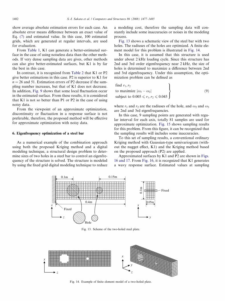
Fig. 13 shows a schematic view of the steel bar with twoholes. The radiuses of the holes are optimized. A finite ele-ment model for this problem is illustrated in Fig. 14.
In this case, it is assumed that this structure is usedunder about 2 kHz loading cycle. Since this structure has2nd and 3rd order eigenfrequency near 2 kHz, the size ofholes is determined to maximize a difference between 2ndand 3rd eigenfrequency. Under this assumption, the opti-mization problem can be defined as
find r1; r2
to maximize jx3 � x2jsubject to 0:005 6 r1; r2 6 0:045
9>=>; ð9Þ
where r1 and r2 are the radiuses of the hole, and x2 and x3
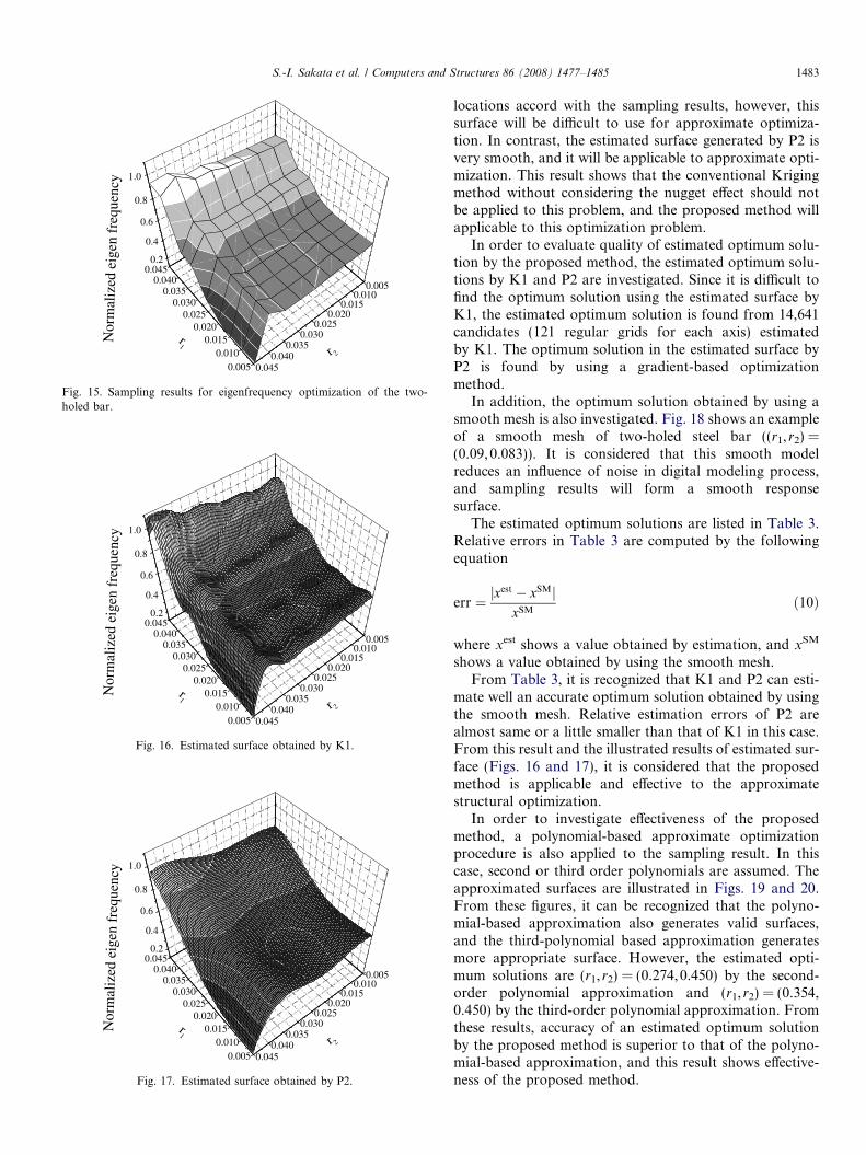
are 2nd and 3rd eigenfrequencies.In this case, 9 sampling points are generated with regu-
lar interval for each axis, totally 81 samples are used forapproximate optimization. Fig. 15 shows sampling resultsfor this problem. From this figure, it can be recognized thatthe sampling results will includes some inaccuracies.
To this set of sampling results, a conventional ordinaryKriging method with Gaussian-type semivariogram (with-out the nugget effect, K1) and the Kriging method basedon the proposed approach (P2) are applied.
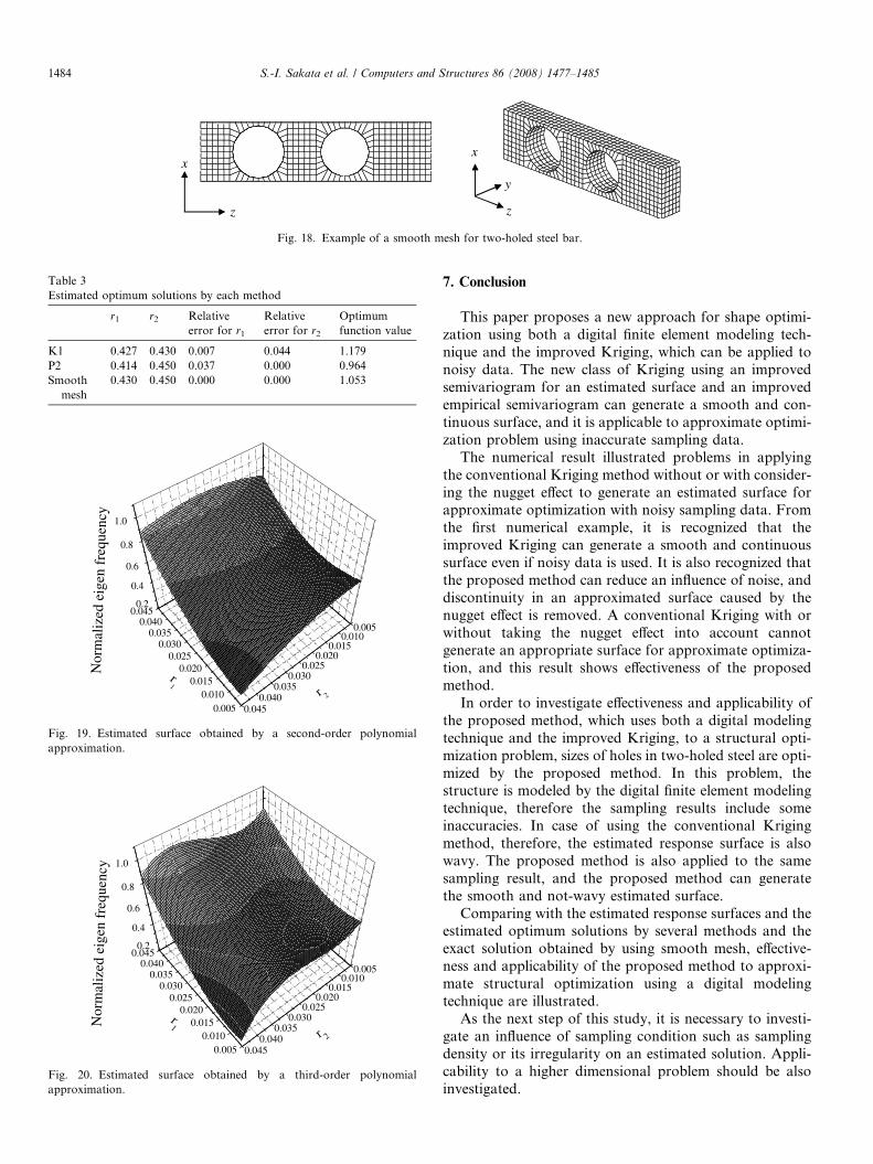
Approximated surfaces by K1 and P2 are shown in Figs.16 and 17. From Fig. 16, it is recognized that K1 generatesa wavy response surface. Estimated values at sampling
y
x0.05m
0.1m Fixed
m
wo-holed steel plate.
x
y
z
t model of a two-holed plate.
0.0050.010
0.0150.020
0.0250.030
0.0350.040
0.0450.0050.010
0.0150.020
0.0250.030
0.0350.040
0.0450.2
0.4
0.6
0.8
1.0
Nor
mal
ized
eig
en f
requ
ency
r1
r 2
Fig. 15. Sampling results for eigenfrequency optimization of the two-holed bar.
0.0050.010
0.0150.020
0.0250.030
0.0350.040
0.0450.0050.010
0.0150.020
0.0250.030
0.0350.040
0.0450.2
0.4
0.6
0.8
1.0
Nor
mal
ized
eig
en f
requ
ency
r1
r 2
Fig. 16. Estimated surface obtained by K1.
0.0050.010
0.0150.020
0.0250.030
0.0350.040
0.0450.0050.010
0.0150.020
0.0250.030
0.0350.040
0.0450.2
0.4
0.6
0.8
1.0
Nor
mal
ized
eig
en f
requ
ency
r1
r 2
Fig. 17. Estimated surface obtained by P2.
S.-I. Sakata et al. / Computers and Structures 86 (2008) 1477–1485 1483
locations accord with the sampling results, however, thissurface will be difficult to use for approximate optimiza-tion. In contrast, the estimated surface generated by P2 isvery smooth, and it will be applicable to approximate opti-mization. This result shows that the conventional Krigingmethod without considering the nugget effect should notbe applied to this problem, and the proposed method willapplicable to this optimization problem.
In order to evaluate quality of estimated optimum solu-tion by the proposed method, the estimated optimum solu-tions by K1 and P2 are investigated. Since it is difficult tofind the optimum solution using the estimated surface byK1, the estimated optimum solution is found from 14,641candidates (121 regular grids for each axis) estimatedby K1. The optimum solution in the estimated surface byP2 is found by using a gradient-based optimizationmethod.
In addition, the optimum solution obtained by using asmooth mesh is also investigated. Fig. 18 shows an exampleof a smooth mesh of two-holed steel bar ((r1, r2) =(0.09, 0.083)). It is considered that this smooth modelreduces an influence of noise in digital modeling process,and sampling results will form a smooth responsesurface.
The estimated optimum solutions are listed in Table 3.Relative errors in Table 3 are computed by the followingequation
err ¼ jxest � xSMj
xSMð10Þ
where xest shows a value obtained by estimation, and xSM
shows a value obtained by using the smooth mesh.From Table 3, it is recognized that K1 and P2 can esti-
mate well an accurate optimum solution obtained by usingthe smooth mesh. Relative estimation errors of P2 arealmost same or a little smaller than that of K1 in this case.From this result and the illustrated results of estimated sur-face (Figs. 16 and 17), it is considered that the proposedmethod is applicable and effective to the approximatestructural optimization.
In order to investigate effectiveness of the proposedmethod, a polynomial-based approximate optimizationprocedure is also applied to the sampling result. In thiscase, second or third order polynomials are assumed. Theapproximated surfaces are illustrated in Figs. 19 and 20.From these figures, it can be recognized that the polyno-mial-based approximation also generates valid surfaces,and the third-polynomial based approximation generatesmore appropriate surface. However, the estimated opti-mum solutions are (r1, r2) = (0.274, 0.450) by the second-order polynomial approximation and (r1, r2) = (0.354,0.450) by the third-order polynomial approximation. Fromthese results, accuracy of an estimated optimum solutionby the proposed method is superior to that of the polyno-mial-based approximation, and this result shows effective-ness of the proposed method.
z
xx
y
z
Fig. 18. Example of a smooth mesh for two-holed steel bar.
Fig. 19. Estimated surface obtained by a second-order polynomialapproximation.
0.0050.010
0.0150.020
0.0250.030
0.0350.040
0.0450.0050.010
0.0150.020
0.0250.030
0.0350.040
0.0450.2
0.4
0.6
0.8
1.0
Nor
mal
ized
eig
en f
requ
ency
r1
r 2
Fig. 20. Estimated surface obtained by a third-order polynomialapproximation.
1484 S.-I. Sakata et al. / Computers and Structures 86 (2008) 1477–1485
7. Conclusion
This paper proposes a new approach for shape optimi-zation using both a digital finite element modeling tech-nique and the improved Kriging, which can be applied tonoisy data. The new class of Kriging using an improvedsemivariogram for an estimated surface and an improvedempirical semivariogram can generate a smooth and con-tinuous surface, and it is applicable to approximate optimi-zation problem using inaccurate sampling data.
The numerical result illustrated problems in applyingthe conventional Kriging method without or with consider-ing the nugget effect to generate an estimated surface forapproximate optimization with noisy sampling data. Fromthe first numerical example, it is recognized that theimproved Kriging can generate a smooth and continuoussurface even if noisy data is used. It is also recognized thatthe proposed method can reduce an influence of noise, anddiscontinuity in an approximated surface caused by thenugget effect is removed. A conventional Kriging with orwithout taking the nugget effect into account cannotgenerate an appropriate surface for approximate optimiza-tion, and this result shows effectiveness of the proposedmethod.
In order to investigate effectiveness and applicability ofthe proposed method, which uses both a digital modelingtechnique and the improved Kriging, to a structural opti-mization problem, sizes of holes in two-holed steel are opti-mized by the proposed method. In this problem, thestructure is modeled by the digital finite element modelingtechnique, therefore the sampling results include someinaccuracies. In case of using the conventional Krigingmethod, therefore, the estimated response surface is alsowavy. The proposed method is also applied to the samesampling result, and the proposed method can generatethe smooth and not-wavy estimated surface.
Comparing with the estimated response surfaces and theestimated optimum solutions by several methods and theexact solution obtained by using smooth mesh, effective-ness and applicability of the proposed method to approxi-mate structural optimization using a digital modelingtechnique are illustrated.
As the next step of this study, it is necessary to investi-gate an influence of sampling condition such as samplingdensity or its irregularity on an estimated solution. Appli-cability to a higher dimensional problem should be alsoinvestigated.
S.-I. Sakata et al. / Computers and Structures 86 (2008) 1477–1485 1485
References
[1] Barthelemy JFM, Haftka RT. Approximation concepts for optimumstructural design – a review. Struct Optimization 1993;5:129–44.
[2] R. Jin, W. Chen, T.W. Simpson, Comparative studies of metamod-eling techniques under multiple modeling criteria, in: AIAA-2000-4801, 2000, pp. 1–11.
[3] E. Nikolaidis, L. Long, Q. Ling, Neural networks and responsesurface polynomials for design of vehicle joints, in: AIAA-98-1777,1998, pp. 653–62.
[4] Sacks J, Welch WJ, Mitchell TJ, Wynn HP. Design and analysis ofcomputer experiments. Stat Sci 1989;4(4):409–35.
[5] Sakata S, Ashida F, Zako M. Structural optimization using Krigingapproximation. Comput Methods Appl Mech Eng 2003;192(7–8):923–39.
[6] Wackernagel H. Multivariate geostatistics. Springer; 2003.[7] Torquato S. Modeling of physical properties of composite materials.
Int J Solid Struct 2000;37:411–22.[8] Bensoe MP, Kikuchi N. Generating optimal topologies in structural
design using a homogenization method. Comput Methods ApplMech Eng 1988;71:197–224.
[9] Terada K, Kikuchi N. Microstructural design of composites using thehomogenization method and digital images. Mater Sci Res Int1996;2(2):65–72.
[10] Cressie N. Fitting variogram models by weighted least squares. MathGeol 1985;17(5):563–86.
[11] Brunell RM, Squibb BM. An Automatic Variogram Fitting Proce-dure Using Cressie’s Criterion. ASA Proceedings of the Section onStatistics and Environment 1993, 135–137.