Approximation of Function and Its Derivatives Using Radial Basis

Approximation of Function and Its Derivatives

Using Radial Basis Function Networks

Nam Mai�Duy and Thanh Tran�Cong�

Faculty of Engineering and Surveying�

University of Southern Queensland� Toowoomba� QLD �� Australia

Submitted to Applied Mathematical Modelling� December �� revised

August ��

Abstract� This paper presents a numerical approach� based on Radial Basis Function

Networks �RBFNs�� for the approximation of a function and its derivatives �scattered

data interpolation�� The approach proposed here is called the indirect radial basis function

network �IRBFN� approximation which is compared with the usual direct approach� In the

direct method �DRBFN� the closed form RBFN approximating function is �rst obtained

from a set of training points and the derivative functions are then calculated directly by

di�erentiating such closed form RBFN� In the indirect method �IRBFN� the formulation

of the problem starts with the decomposition of the derivative of the function into RBFs�

�Corresponding author� Telephone �� Fax �� E mail trancong�usq�edu�au

�

The derivative expression is then integrated to yield an expression for the original function�

which is then solved via the general linear least squares principle� given an appropriate

set of discrete data points� The IRBFN method allows the �ltering of noise arisen from

the interpolation of the original function from a discrete set of data points and produces a

greatly improved approximation of its derivatives� In both cases the input data consists of

a set of unstructured discrete data points �function values�� which eliminates the need for

a discretisation of the domain into a number of �nite elements �FE�� The results obtained

are compared with those obtained by the Feed Forward Neural Network �FFNN� approach

where appropriate and the Finite Element methods� In all examples considered� the

IRBFN approach yields a superior accuracy� For example� all partial derivatives up to

second order of the function of three variables y � x�� x�x� � �x�� x�x� � x�� are

approximated with at least an order of magnitude better in the L� norm in comparison

with the usual DRBFN approach�

Keywords� Radial basis function networks� function approximation� derivative approxi

mation� scattered data interpolation� global approximation�

� Introduction

Numerical methods for di�erentiation are of signi�cant interest and importance in the

study of numerical solutions of many problems in engineering and science� For example�

the approximation of derivatives is needed either to convert the relevant governing equa

tions into a discrete form or to numerically estimate various terms from a set of discrete

or scattered data� This is commonly achieved by discretising the domain of analysis into

a number of elements which are de�ned by a small number of nodes� The interpolation

of a function and its derivatives over such an element from the nodal values can then be

achieved analytically via the chosen shape functions� Examples of elements include �nite

elements �FE� and boundary elements �BE� associated with the Finite Element Method

�FEM� �e�g� �� and the Boundary Element Method �BEM� �e�g� �� Element based

methods are referred to as conventional methods in this paper� Common shape functions

for one� two and three dimensional elements can be found in most texts on Finite Ele

mentMethod and Boundary ElementMethod �e�g� �� However� the element technique

requires mesh generation which is time consuming and therefore accounts for a high pro

portion of the analysis cost� especially for problems with moving or unknown boundaries�

For practical analysis� automatic discretisation or meshing is a highly desirable feature

but rarely available in general� Thus there are great interests in element free numerical

methods in both engineering and scienti�c communities� In particular� neural networks

have been developed and become one of the main �elds of research in numerical analysis�

Radial Basis Function Networks �RBFNs� �� can be used for a wide range of applica

tions primarily because it can approximate any regular function �� and its training

is faster than that of a multilayer perceptron when the RBFN combines self organised

and supervised learning �� The design of an RBFN is considered as a curve �tting �ap

proximation� problem in a high dimensional space� Correspondingly� the generalization

of the approach is equivalent to the use of a multidimensional surface to interpolate the

test data �� The networks just need an unstructured distribution of collocation points

throughout a volume for the approximation and hence the need for discretisation of the

volume of the analysis domain is eliminated� In this paper new approximation methods

based on RBFNs are reported� The primary aim of the presented methods is the achieve

ment of a more accurate approximation of a target function�s derivatives� From the results

obtained here it is suggested that the present IRBFN approach could be� in addition to

its ability to approximate scattered data� a potential candidate for future development

of element free methods for engineering modelling and analyses� The paper is organized

as follows� In section �� the problem is de�ned� A brief review of RBFNs is given in

section � and then� in sections � and �� a direct RBFN �DRBFN� and an indirect RBFN

�IRBFN� method for the approximation of a function and its derivatives are discussed�

The DRBFN method is included to provide the basis for the assessment of the presently

proposed IRBFN approach� Both methods are illustrated with the aid of three numerical

examples of function of one� two and three variables in section �� Section � concludes the

paper�

� Description of Problem

The problem considered in this paper is described as follows �superscripts are used to index

elements of a set of neurons and subscripts denote scalar components of a p dimensional

vector��

� Given a set of data points whose elements consist of paired values of the indepen

dent variables �a vector x� and the dependent variable �a scalar y�� denoted by

fx�i�� y�i�gni�� where n is the number of input points and x � �x�� x�� xp�T where p

is the number of dimensions and the superscript T denotes the transpose operation�

� �nd a closed form approximate function f of the dependent variable y and its closed

form approximate derivative functions�

� Function Approximation by RBFNs

An RBFN represents a map from the p dimensional input space to the � dimensional

output space f � Rp � R� that consists of a set of weights fw�i�gmi�� and a set of radial

basis functions fg�i�gmi�� where m � n� There is a large class of radial basis functions

which can be written in a general form g�i��x� � ��i��kx � c�i�k�� where k�k denotes the

Euclidean norm and fc�i�gmi�� is a set of the centers that can be chosen from among the

data points� The following are some common types of radial basis functions that are of

particular interest in the study of RBFNs ��

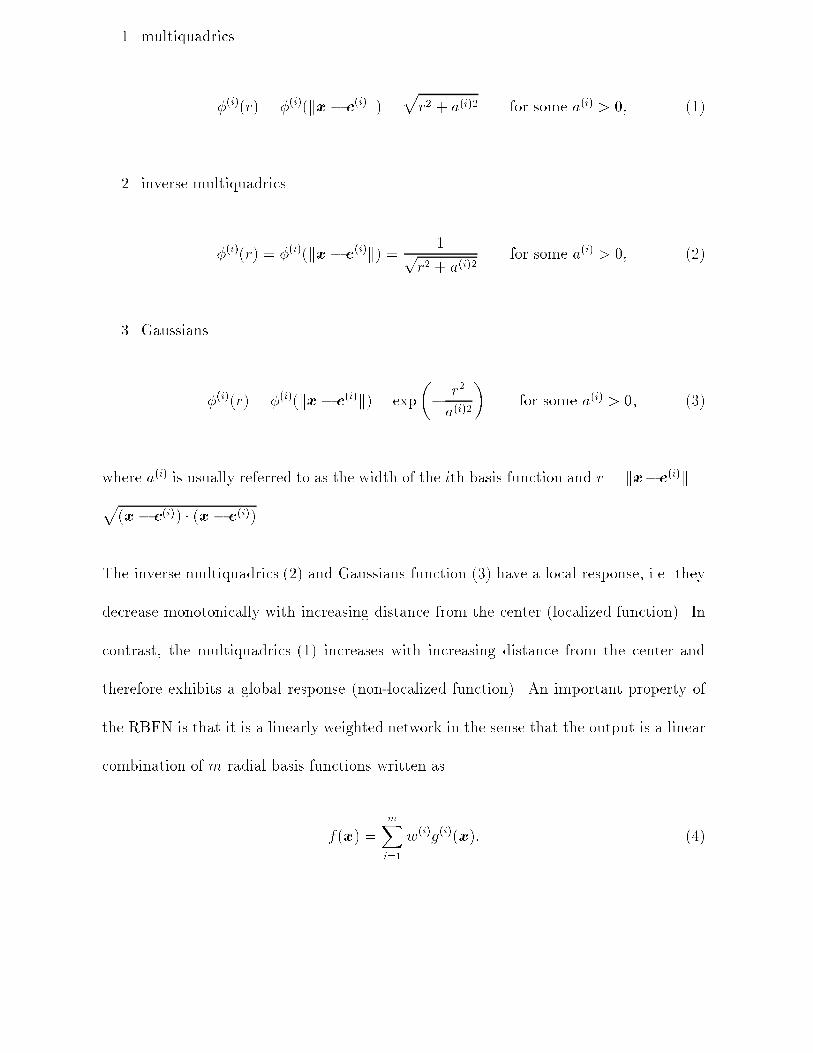
�� multiquadrics

��i��r� � ��i��kx� c�i�k� �pr� � a�i�� for some a�i� � ��

�� inverse multiquadrics

��i��r� � ��i��kx� c�i�k� � �pr� � a�i��

for some a�i� � ��

�� Gaussians

��i��r� � ��i��kx� c�i�k� � exp

�� r�

a�i��

�for some a�i� � ��

where a�i� is usually referred to as the width of the ith basis function and r � kx�c�i�k �p�x� c�i�� x� c�i��

The inverse multiquadrics �� and Gaussians function �� have a local response� i�e� they

decrease monotonically with increasing distance from the center �localized function�� In

contrast� the multiquadrics �� increases with increasing distance from the center and

therefore exhibits a global response �non localized function�� An important property of

the RBFN is that it is a linearly weighted network in the sense that the output is a linear

combination of m radial basis functions written as

f�x� �mXi��

w�i�g�i��x��

With the model f constructed as a linear combination of m �xed functions in a given

family� the problem is to �nd the unknown weights fw�i�gmi�� For this purpose� the general

least squares principle is used to minimise the sum squared error

SSE �

nXi��

�y�i� � f�x�i��

��

with respect to the weights of f � resulting in a set of m simultaneous linear algebraic

equations �normal equations� in the m unknown weights

�GTG�w � GTy� ��

where

G �

��

g��x�� g��x�� g�m��x��

g��x�� g��x�� g�m��x��

��

� � ��

g��x�n�� g��x�n�� g�m��x�n��

��

w � �w�� w�� w�m��T �

y � �y�� y�� y�n��T �

However� in the special case where n � m� the resultant system is just

Gw � y� ��

� Function derivatives by direct RBFN method

In an arbitrary RBFN where the basis functions are �xed and the weights are adaptable�

the derivative of the function computed by the network is also a linear combination of

�xed functions �the derivatives of the radial basis functions�� The partial derivatives of

the approximate function f�x� �� can be calculated as follows

�kf

�xj��xl� f�j��l�x� �

mXi��

w�i� �kg�i�

�xj��xl� ��

where �kg�i�

�xj��xlis the corresponding basis function for the derivative function f�j��l�x�� which

is obtained by di�erentiating the original basis function g�i��x� which is continuously

di�erentiable� For example� considering the �rst order derivative of function f�x� with

respect to xj� denoted by f�j� the corresponding basis functions are found analytically as

follows�

�� for multiquadrics

h�i��x� ��g�i�

�xj�

xj � c�i�j

�r� � a�i��

�� for inverse multiquadrics

h�i��x� ��g�i�

�xj� � xj � c

�i�j

�r� � a�i��

�� for Gaussians

h�i��x� ��g�i�

�xj��xj � c

�i�j �

a�i��exp

�� r�

a�i��

��

Considering the second order derivative of function f�x� with respect to xj� denoted by

f�jj� the corresponding basis functions will be


�h�i��x� ��h�i�

�xj�r� � a�i�� xj � c

�i�j ��

�r� � a�i��


�h�i��x� ��h�i�

�xj�

��xj � c�i�j ��

�r� � a�i��

�r� � a�i��


�h�i��x� ��h�i�

�xj�

�

a�i��

��

a�i��xj � c

�i�j ��

exp

�� r�

a�i��

��

Similarly� the basis functions for f�kj are as follows�


�h�i��x� ��h�i�

�xk� ��xj � c

�i�j ��xk � c

�i�k �

�r� � a�i��


�h�i��x� ��h�i�

�xk�

��xj � c�i�j ��xk � c

�i�k �

�r� � a�i��


�h�i��x� ��h�i�

�xk�

��xj � c�i�j ��xk � c

�i�k �

a�i�exp

�� r�

a�i��

��

Once f�x� is determined by solving �� or �� for the unknown weights� which is referred

to as network training� it is straightforward and economical to compute its derivatives

according to �� However� this direct method has some drawbacks that are illustrated in

the following example�

�� Example to illustrate the drawbacks of the DRBFN method

The function

y�x� � x� � x� �� x � ��

is sampled at �� uniformly spaced training points as depicted in Figure �� Parameters

to be decided before the start of network training are the number of centers m� their

locations fc�i�gmi�� and a set of the corresponding widths fa�i�gmi�� The ideal data points

used here are not corrupted by noise� According to Cover�s Theorem �� the more basis

functions are used� the better the approximation will be and so all data points will be

taken to be the centers of the network �m � n� in this study� Thus fc�i� � x�i�gni�� The

width of the ith basis function is determined according to the following relation ��

a�i� � �d�i��

where � is a factor� � � �� and d�i� is the distance from the ith center to the nearest

neighbouring center� As a measure of the accuracy of di�erent approximate schemes� a

norm of the error of the solution� Ne� is de�ned as

Ne �

vuut ntXi��

�y�i� � f �i��

where f �i� and y�i� are the calculated and exact function values at the point i� and nt is

the total number of test nodes� Smaller Nes indicate more accurate approximations�

Table � shows the error norms Nes of the approximate function and its �rst and sec

ond derivatives that are obtained from the networks using di�erent types of radial basis

function based on a set of �� test nodes� It can be seen that errors in the approximate

function obtained from all networks are quite low and hence the global shape of the orig

inal function is well captured as shown in Figure �� However� the derivative functions�

especially higher order ones� are strongly in�uenced by the local behaviour of the ap

proximant� The nature of a bad local behaviour despite a good global approximation is

illustrated in Figure �a� The errors in the function approximation amplify in the process

of di�erentiation as shown in Figures �b c with the corresponding error norms Nes shown

in Table �� It is remarkable that multiquadrics RBFs �� produce greater accuracy than

other basis functions� This surprising result was discussed by Franke �� and Powell ��

However� the norms Nes of the derivative functions estimated using multiquadrics RBFs

are still quite high �Table �� To improve accuracy� a new indirect method is proposed

and presented in the next section�

� Function derivatives by indirect RBFN method

It can be seen that the di�erentiation process is very sensitive to even a small level of

noise as illustrated in the previous section� In contrast it is expected that on average

the integration process is much less sensitive to noise� Based on this observation� it is

proposed here that the approximation procedure starts with the derivative function using

RBFNs� The original function is then obtained by integration� Here the generic nature of

derivative function and original function is illustrated as follows� Suppose a function

f�x� and its derivatives f ��x� and f ��x� are to be approximated� The procedure consists

of two stages� In the �rst stage� f�x� corresponds to the original function and f ��x� the

derivative function� In the second stage the f ��x� obtained in stage � corresponds to

the original function and f ��x� the derivative function� The procedure just discussed

is here referred to as the �rst indirect method or IRBFN�� Alternatively� the procedure

can start with the second derivative� First� the second order derivative is approximated

by a RBFN� then the �rst order derivative is obtained by integration� Finally the original

function is similarly obtained� i�e� by integrating the �rst derivative function� This

second method is here referred to as the second indirect method or IRBFN�� The detail

of IRBFN� and IRBFN� is described in the next two sections for function of one and two

or more variables respectively� followed by some numerical results in section ��

�� Functions of one variable

�� IRBFN� method

In this method� the �rst order derivative function is decomposed into radial basis functions

as

f ��x� �

mXi��


where fg�i��x�gmi�� is a set of radial basis functions and fw�i�gmi�� is the set of corresponding

weights� With this approximation� the original function can be calculated as

f�x� �

Zf ��x�dx �

Z mXi��

w�i�g�i��x�dx �mXi��

w�i�

Zg�i��x�dx �

mXi��

w�i�H�i��x� � C��

��

where C� is the constant of integration and fH�i��x�gmi�� is the set of corresponding basis

functions for the original function with H�i��x� �Rg�i��x�dx� The radial basis functions

fg�i�gmi�� are continuously integrable� but only two basis functions fH�i��x�gmi�� corre

sponding to the multiquadric �� and the inverse multiquadric �� are able to be obtained

analytically here� This paper focuses on the use of these two RBFs in the indirect method�

The corresponding basis functions are�


H�i��x� ��x� c�i��

p�x� c�i�� a�i��

��a�i��

�ln

��x� c�i��

q�x� c�i�� a�i��

��

��


H�i��x� � ln

��x� c�i��

q�x� c�i�� a�i��

��

The training to determine the weights in �� and �� is equivalent to a minimisation of

the following sum squared error

SSE �nXi��

�y�i� � f�x�i��

��

Equation �� is used in equation �� in the minimisation procedure� which results in a

system of equations in terms of the unknown weights w�i�� The data used in training the

network for the derivative and original functions just consists of a set of discrete values

fy�i�gni�� of the dependent variable y and the closed form of the derivative function ��

The minimisation of �� can be achieved by solving the corresponding normal equations

�� However in practice the normal equations method of solution can produce less than

optimum solution� i�e� the norm of the solution �in the least square sense� is not the

smallest� Fortunately� Singular Value Decomposition �SVD� method �� can overcome

this di�culty and will be used to solve �� for the unknown weights and the constant of

integration in the remainder of this paper� The SVD method provides a solution whose

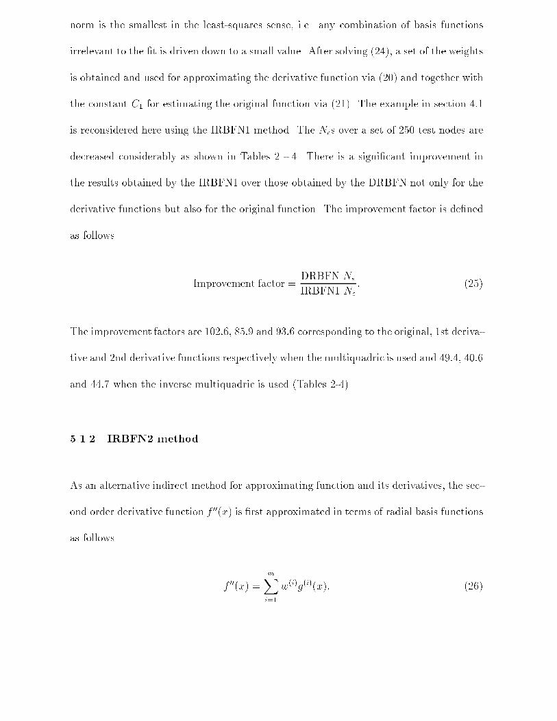
norm is the smallest in the least squares sense� i�e� any combination of basis functions

irrelevant to the �t is driven down to a small value� After solving �� a set of the weights

is obtained and used for approximating the derivative function via �� and together with

the constant C� for estimating the original function via �� The example in section ��

is reconsidered here using the IRBFN� method� The Nes over a set of �� test nodes are

decreased considerably as shown in Tables � �� There is a signi�cant improvement in

the results obtained by the IRBFN� over those obtained by the DRBFN not only for the

derivative functions but also for the original function� The improvement factor is de�ned

as follows

Improvement factor �DRBFN Ne

IRBFN� Ne

� ��

The improvement factors are �� and �� corresponding to the original� �st deriva

tive and �nd derivative functions respectively when the multiquadric is used and ��

and �� when the inverse multiquadric is used �Tables � ��


As an alternative indirect method for approximating function and its derivatives� the sec

ond order derivative function f ��x� is �rst approximated in terms of radial basis functions

as follows

f ��x� �mXi��


Then the �rst derivative function f ��x� is given by �� as

f ��x� �

Zf ��x�dx �

mXi��

w�i�H�i��x� � C��

with the basis functions given by �� or �� The original function is calculated as

f�x� �

Zf ��x�dx �

mXi��

w�i� �H�i��x� � C�x� C��

where C� and C� are constants of integration and the corresponding basis functions are

obtained by integrating �� or �� as shown below


�H�i��x� �

ZH�i��x�dx �

��x� c�i�� a�i��

��

a�i��

��x� c�i�� ln

��x� c�i��

q�x� c�i�� a�i��

�� a�i��

�

q�x� c�i�� a�i��


�H�i��x� �

ZH�i��x�dx � �x� c�i�� ln

��x� c�i��

q�x� c�i�� a�i��

�

�q�x� c�i�� a�i��

In the present IRBFN� method� the improvement factors have increased �Tables � �� for

both the original function and its derivatives in comparison with the �rst indirect method

IRBFN�� It is remarkable here that the improvement in the case of multiquadrics is very

signi�cant for all approximate functions �more than �� times�� Thus� the multiquadric

function maintains its superior performance in terms of accuracy among the radial basis

functions used in IRBFN��

�� The role of �constants� of integration

Constants of integration in equations �� and �� appear naturally in the present

indirect formulation� The structure of the approximant therefore looks like

f�x� �mXi��

w�i� �H�i��x� � polynomial� ��

As a result� if y�x� is �at or closer to a polynomial �t� the above structure �� has the

ability for better accuracy� This is in addition to the inherent smoothing of error in the

process of integration�

�� Functions of two or more variables

In this section the indirect methods discussed in section �� are extended to the case of

functions of many variables� The case of functions of two variables is discussed in detail

and the procedure for functions of three or more variables can be similarly developed�


Consider the approximation of a function of two variables f�x�� x�� In the IRBFN�

method� the �rst order partial derivative of f�x�� x�� with respect to x�� denoted by f��

is �rst approximated in terms of radial basis functions

f��x�� x�� mXi��

w�i�g�i��x�� x��

where fg�i��x�� x��gmi�� is a set of radial basis functions and fw�i�gmi�� is the set of corre

sponding weights�

The original function can be calculated as

f�x�� x��

Zf��x�� x��dx� �

Z mXi��

w�i�g�i��x�� x��dx�

�mXi��

w�i�

Zg�i��x�� x��dx� �

mXi��

w�i�H�i��x�� x�� C��x��

where C��x�� is a function of the variable x� and fH�i��x�� x��gmi�� is the set of correspond

ing basis functions for the original function and given below


H�i��x�� x�� x� � c

�i�� pr� � a�i��

�

�r� � �x� � c

�i�� a�i��

�ln��x� � c

�i��

pr� � a�i��

��


H�i��x�� x�� ln��x� � c

�i��

pr� � a�i��

��

The added term on the right hand side of �� is a function of the variable x� only� Thus

C��x�� can be interpolated using the IRBFN� method for univariate functions as follows

�in the previous section� IRBFN� is shown to be the better alternative among the methods

investigated in this work��

C ��

� �x��

MXi��

�w�i�g�i��x��

C �

��x�� MXi��

�w�i�H�i��x�� bC��

C��x�� MXi��

�w�i� �H�i��x�� bC�x� � bC��

where bC� and bC� are constants of integration� �w�i� are the corresponding weights� andM is

the number of centres whose x� coordinates are distinct� Upon applying the general linear

least squares principle� a system of linear algebraic equations is obtained� The unknown

of the system which is found by the SVD method as mentioned earlier� consists of the

set of weights in �� the second set of weights in �� and the constants of integration

bC�� bC�� The strategy of approximation is the same for the derivative function of f�x�� x��

with respect to the variable x� �f��x�� x��


In this method� the second order derivative functions are �rst approximated in terms of

radial basis functions� For example� in the case of f�� the basis functions for the �rst

derivative function� f�� are given by �� or �� while for the original function f � the

basis functions are obtained by integrating �� or �� and shown below


�H�i��x�� x��

ZH�i��x�� x��dx� �

�r� � a�i��

��

r� � �x� � c�i�� a�i��

��x� � c�� ln

��x� � c

�i��

pr� � a�i��

��

r� � �xj � c�i�j �� a�i��

�

pr� � a�i��


�H�i��x�� x��

ZH�i��x�� x��dx� �

�x� � c�� ln��x� � c

�i��

pr� � a�i��

��pr� � a�i��

The original function is calculated as

f�x�� x�� mXi��

w�i�H�i��x�� x�� C��x��x� � C��x��

where C��x�� and C��x�� are constants of integration which are interpolated in the same

maner as shown by ��

For the purpose of illustration� some numerical results are presented in the next section�

� Numerical results

In this section� examples of approximation of functions of one� two and three variables

are given� As mentioned� the multiquadric function appears to be the better one in terms

of accuracy among the basis functions considered and will be used to solve the example

problems� The factor � that in�uences the accuracy of the solution is just chosen to be ��

until now� In the following examples� for the purpose of investigation of its e�ect� � will

take values over a wide range with an increment of �� From the numerical experiments

discussed shortly� it appears that there is an upper limit for � above which the system

of equations �� or �� is ill conditioned� which is also observed by Tarwater �� In the

present work� the value of � is considered to reach an upper limit when the condition of

the system matrix is O�� i�e� the estimate for the reciprocal of the condition of the

matrix in � norm using LINPACK condition estimator �� is of O��

�� Example �

Consider the following function of one variable

y � �� x� ��x� � ��x�� cos ��x�� sin ��x��

with � � x � �� a problem studied by Hashem and Schmeiser �� They reported a

method� namely Mean Squared Error Optimal Linear Combinations of Trained Feedfor

ward Neural Netwoks �MSE OLC�� for an approximation of the function and its deriva

tives� The authors suggest that the usual approach is to try a multiple of networks

with possibly di�erent structures and values for training parameters and the best net

work �based on some optimality criterion� is selected� Instead of the usual approach just

described the authors investigated a new approach where a combination of the trained

networks is constructed by forming the weighted sum of the corresponding outputs of

the trained networks� The authors claim that their MSE OLC method yields more accu

rate approximations in comparison with the best trained FFNN� For this problem� with

a set of �� training nodes and �� test nodes� the resultant MSEs for the original�

the �rst and second order derivative functions produced by MSE OLC are ��

and �� respectively� which are �� and �� respectively� less than the

MSEs produced by the best FFNN �� Here� both the direct and indirect RBFN meth

ods are applied to solve this problem using �� training points and �� test nodes�

uniformly spaced along the x axis� The training points are displayed in Figure �a� In

contrast� Hashem and Schmeiser �� used the same number of data points but randomly

distributed� In order to compare the present results with those obtained by Hashem and

Schmeiser �� the latter�s MSEs are converted into norms Nes as de�ned in this paper�

Thus the norms Nes corresponding to the original� �rst derivative and second derivative

are �� and �� respectively� Figure � compares the quality of approximation

obtained by the DRBFN� IRBFN�� IRBFN�� MSE OLC and the conventional element

method �with linear element� in the range �� and indicates that the quality

of approximation improves signi�cantly with RBFN� and particularly that the IRBFN�

yields superior results over the whole range of values of � �e�g� with � � � the Nes

for the second derivative are �� IRBFN�� DRBFN�� conventional�

and �� MSE OLC� �� Even more accurate results can be obtained by using the

second indirect method IRBFN� �Ne � �� as shown in the same Figure �� Figure �

shows the plots of the function and its derivative at � � �� obtained with the IRBFN�

where the worst value of � is used to demonstrate the superior performance of the

IRBFN��

�� Example �

Consider the following bivariate function

y � x��x� � x�� x��

where �� x� � � and �� x� � �� This is a non trivial example which has a

complicated root structure �� The data consist of �� points� uniformly spaced along

both axes x� and x� for training and �� points for testing� The results obtained from

both DRBFN and IRBFN methods are compared with the accuracies achieved by the

conventional method using linear shape function over triangular elements� Figure � shows

the quality of the approximation of the function f�x�� x�� and its �rst derivatives while

Figure � shows the quality of the approximation of second order derivatives using the

DRBFN� IRBFN� and IRBFN� with � in the range �� Again� the results

are more accurate with IRBFN� as shown in Figures � �� Thus it can be seen that the

IRBFN� yields better performance than the IRBFN� which in turn performs better than

the DRBFN�

�� Example �

Consider the following function of three variables

y � x�� x�x� � �x�� x�x� � x��

where � � x� � �� x� � �� and � � x� � �� In this example� �� points�

uniformly spaced along the axes x�� x� and x�� are used for training and �� points for

testing� Figure � shows the quality of the approximation of the original function� Figure

� shows the plots of norm Ne as function of � �� for �rst order derivative

functions f�� f�� and f�� while Figures � �� are for second order derivative functions f��

f�� f�� f�� f�� and f�� Figures � �� again show that the IRBFN� method exhibits

superior performance over other methods�

� Concluding Remarks

This paper reports the successful development and implementation of function approxi

mation methods based on RBFNs for functions of one� two and three variables and their

derivatives �scattered data interpolation�� Both the direct RBFN method and the indi

rect RBFN method are able to o�er better results in comparison with the conventional

method using linear shape functions� The present RBFN methods also eliminate the

need for FE type discretisation of the domain of analysis� Among the RBFs considered�

multiquadrics RBF o�ers the best performance in accuracy in both DRBFN and IRBFN

method� Numerical results show that IRBFNs� especially IRBFN�� achieve greater accu

racy than DRBFN in the approximation of both function and especially its derivatives�

Furthermore� this superior accuracy is maintained over a wide range of RBF�s width

�� A formal theoretical proof of the superior accuracy of the present IRBFN

method cannot be o�ered at this stage� at least by the present authors� However� a

heuristic argument can be presented as follows� In the direct methods� the starting point

is the decomposition of the unknown functions into some �nite basis and all derivatives

are obtained as a consequence� Any inaccuracy in the assumed decomposition is usually

magni�ed in the process of di�erentiation� In contrast� in the indirect approach the start

ing point is the decomposition of the highest derivatives into some �nite basis� Lower

derivatives and �nally the function itself are obtained by integration which has the prop

erty of damping out or at least containing any inherent inaccuracy in the assumed shape

of the derivatives� At this stage� it is recommended that the IRBFN� method is the better

one among the methods considered for an accurate approximation of a function and its

derivative� In a subsequent study� the application of the DRBFN and IRBFN methods in

solving di�erential equations will be reported�

Acknowledgements

This work is supported by a Special USQ Research Grant to Thanh Tran Cong �Grant No

�� Nam Mai Duy is supported by a USQ scholarship� This support is gratefully

acknowledged� The authors would like to thank the referees for their helpful comments�

References

�� R�D� Cook� D�S� Malkus� M�E� Plesha� Concepts and Applications of Finite Element

Analysis� John Wiley � Sons� Toronto� ��

�� C�A� Brebbia� J�C�F� Telles� L�C� Wrobel� Boundary Element Techniques� Theory

and Applications in Engineering� Springer Verlag� Berlin� ��

�� M�J�D� Powell� Radial basis functions for multivariable interpolation� a review� in�

J�C� Watson� M�G� Cox �Eds�� IMA Conference on Algorithms for the Approxima

tion of Function and Data� Royal Military College of Science� Shrivenham� England�

�� pp� ��

� D�S� Broomhead� D� Lowe� Multivariable functional interpolation and adative net

works� Complex Systems � ��

�� M�J�D� Powell� Radial basis function approximations to polynomial� in� D�F� Gri�ths�

G�A� Watson �Eds�� Numerical Analysis �� Proceedings� University of Dundee�

Dundee� UK� �� pp� ��

�� T� Poggio� F� Girosi� Networks for approximation and learning� in� Proceedings of

the IEEE �� pp��

�� F� Girosi� T� Poggio� Networks and the best approximation property� Biological Cy

bernetics ��

� S� Chen� F�N� Cowan� P�M� Grant� Orthogonal least squares learning algorithm for

radial basis function networks� IEEE Transaction on Neural Networks � ��

��

�� S� Haykin� Neural Networks� A Comprehensive Foundation� Prentice Hall� New Jer

sey� ��

�� J� Park� I�W� Sandberg� Approximation and radial basis function networks� Neural

Computation � ��

�� J� Moody� C�J� Darken� Fast learning in networks of locally tuned processing units�

Neural Computation � ��

�� R� Franke� Scattered data interpolation� tests of some methods� Mathematics of

Computation ��

�� W�H� Press� B�P� Flannery� S�A� Teukolsky� W�T� Vetterling� Numerical Recipes in

C� The Art of Scienti�c Computing� Cambridge University Press� Cambridge� ��

�� A�E� Tarwater� A parameter study of Hardy�s multiquadrics method for scattered

data interpolation� Technical Report UCRL �� Lawrence Livemore National

Laboratory� ��

�� J�J� Dongarra� J�R� Bunch� C�B� Moler� G�W� Stewart� LINPACK User�s Guide�

SIAM� Philadelphia� ��

�� S� Hashem� B� Schmeiser� Approximating a function and its derivatives using MSE

optimal linear combinations of trained feedforward neural networks� in� Proceedings

of the �� World Congress on Neural Networks� vol �� Lawrence Erlbaum Asso

ciates� Hillsdale� New Jersey� �� pp� ��

�� S�V� Chakravarthy� J� Ghosh� Function emulation using radial basis function net

works� Neural Networks ��

Table �� Ne of the approximate function and its derivatives for � � �� with the di rect RBFN �DRBFN� approach� The quality of approximation deteriorates with higherderivatives�

Gaussians multiquadrics Inverse multiquadricsOriginal function ��e� �� e� �� e � ��st derivative ��e� �� e� �� e � ��nd derivative ��e� �� e� �� e � ��

Table �� Comparison of Nes between the DRBFN and IRBFN� for the original function��

multiquadrics Inverse multiquadricsDRBFN ��e � �� e � ��IRBFN� ��e � �� e � ��Improvement factor ��

Table �� Comparison of Nes between the DRBFN and IRBFN� for the �st derivativefunction� � � ��

multiquadrics Inverse multiquadricsDRBFN ��e� �� e � ��IRBFN� ��e � �� e � ��Improvement factor ��

Table �� Comparison of Nes between the DRBFN and IRBFN� for the �nd derivativefunction� � � ��

multiquadrics Inverse multiquadricsDRBFN ��e� �� e � ��IRBFN� ��e� �� e � ��Improvement factor ��

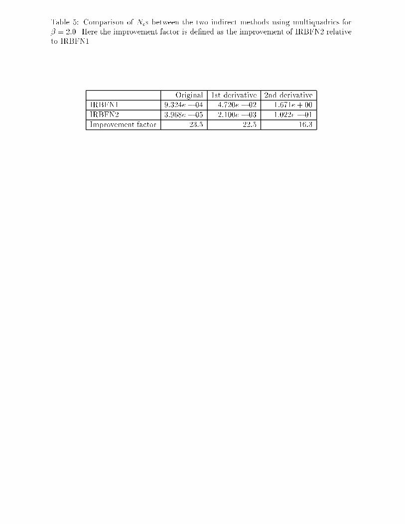
Table �� Comparison of Nes between the two indirect methods using multiquadrics for� � �� Here the improvement factor is de�ned as the improvement of IRBFN� relativeto IRBFN��

Original �st derivative �nd derivativeIRBFN� ��e � �� e � �� e � ��IRBFN� ��e � �� e � �� e � ��Improvement factor ��

Table �� Comparison of Nes between the two indirect methods using inverse multiquadricsfor � � �� Here the improvement factor is de�ned as the improvement of IRBFN�relative to IRBFN��

Original �st derivative �nd derivativeIRBFN� ��e � �� e � �� e � ��IRBFN� ��e � �� e � �� e � ��Improvement factor ��

−3 −2.5 −2 −1.5 −1 −0.5 0 0.5 1 1.5 2−30

−25

−20

−15

−10

−5

0

5

10

15

training pointexactapproximate

x

y�f

Figure �� Function y�x� � x� � x � �� plot of training points� the exact function andthe approximate function obtained by the direct RBFN using inverse multiquadrics basisfunctions �DRBFN� with � � �� Note that the accuracy of the approximation of thefunction is such that the error �i�e� the di�erence between the dashed and the solid lines�is not discernible on this plot� However� the goodness of the global shape might not begood enough in obtaining accurate function derivatives as illustrated in the next Figure��

1.75 1.8 1.85 1.9 1.95 27.5

8

8.5

9

9.5

10

10.5

11

1.75 1.8 1.85 1.9 1.95 20

5

10

15

20

1.75 1.8 1.85 1.9 1.95 2−400

−300

−200

−100

0

100

200

x

y�f

y��f�

y��f��

a� Original function

b� First derivative

c� Second derivative

Figure �� Function y�x� � x�� x� �� Zoom in on the original� �rst derivative and sec ond derivative functions �� Solid line� exact function and dashed line� DRBFNapproximation using inverse multiquadrics� The plots illustrate the shortcomings of theDRBFN approach where the associated error norms are ��e�� e�� and ��e��for the approximation of the function� its �rst derivative and second derivative respec tively�

0 1 2 3 4 5 6 7 8 910

−8

10−6

10−4

10−2

100

0 1 2 3 4 5 6 7 8 910

−6

10−4

10−2

100

102

0 1 2 3 4 5 6 7 8 910

−2

100

102

104

106

�

Ne

Ne

Ne

a� Quality of f

b� Quality of f �

c� Quality of f ��

Figure �� Approximant f of the function y � ��x��x��x��cos ��x�� sin ��x� and its derivatives� plots of the norm Ne as a function of �� Legends �� MSE OLC� x� conventional element method� solid line� DRBFN� dashdot line� IRBFN� anddashed line� IRBFN��

0 0.1 0.2 0.3 0.4 0.5 0.6 0.7 0.8 0.9 10

0.2

0.4

0.6

0.8

1

0 0.1 0.2 0.3 0.4 0.5 0.6 0.7 0.8 0.9 1−6

−4

−2

0

2

4

6

8

0 0.1 0.2 0.3 0.4 0.5 0.6 0.7 0.8 0.9 1−150

−100

−50

0

50

100

x

y�f

y��f�

y��f��

a� Original function

b� First derivative

c� Second derivative

Figure �� Function y � �� x� ��x��x�� cos ��x�� sin ��x� and itsderivatives� plots of function and its derivatives at the worst value of � �� Dashedline� exact and dashdot line� IRBFN�� The quality of the IRBFN� approximation is suchthat the numerical approximation and the analytical plots are not discernible� The datapoints are also shown as ��

0 1 2 3 4 5 6 710

−4

10−3

10−2

10−1

100

101

0 1 2 3 4 5 6 710

−3

10−2

10−1

100

101

102

0 1 2 3 4 5 6 710

−4

10−2

100

102

�

Ne

Ne

Ne

a� Quality of f

b� Quality of f��

c� Quality of f��

Figure �� Approximant f of the function y�x�� x�� x��x��x��x

�� and its derivatives�

plots of the norm Ne as a function of �� Legends x� conventional element method� solidline� DRBFN� dashdot line� IRBFN� and dashed line� IRBFN�� It can be seen that thequality of the approximation for the derivatives is much better with the IRBFN approach�

0 1 2 3 4 5 6 710

−4

10−2

100

102

104

0 1 2 3 4 5 6 710

−4

10−2

100

102

104

0 1 2 3 4 5 6 710

−4

10−2

100

102

�

Ne

Ne

Ne

a� Quality of f��



Figure �� Approximant of the derivatives of the function y�x�� x�� x��x� � x�� x��plots of the norm Ne as a function of �� Legends x� conventional element method� solidline� DRBFN� dashdot line� IRBFN� and dashed line� IRBFN�� It can be seen that thequality of the approximation for the derivatives is much better with the IRBFN approach�

0 1 2 3 4 5 6 7 810

−4

10−3

10−2

10−1

100

�

Ne

a� Quality of f

Figure �� Approximant of the function y � x�� x�x� � �x�� x�x� � x�� plots of thenorm Ne as a function of �� Solid line� DRBFN� dashdot line� IRBFN� and dashed line�IRBFN�� It can be seen that the quality of the approximation is much better with theIRBFN approach�

0 1 2 3 4 5 6 7 810

−3

10−2

10−1

100

101

0 1 2 3 4 5 6 7 810

−3

10−2

10−1

100

101

0 1 2 3 4 5 6 7 810

−3

10−2

10−1

100

101

�

Ne

Ne

Ne




Figure �� Approximant of the derivatives of the function y � x��x�x�� x��x�x��x��plots of the norm Ne as a function of �� Legends x� conventional element method� solidline� DRBFN� dashdot line� IRBFN� and dashed line� IRBFN�� It can be seen that thequality of the approximation is much better with the IRBFN approach�

0 1 2 3 4 5 6 7 810

−1

100

101

102

103

0 1 2 3 4 5 6 7 810

−1

100

101

102

103

0 1 2 3 4 5 6 7 810

−1

100

101

102

103

�

Ne

Ne

Ne




Figure �� Approximant of the derivatives of the function y � x��x�x�� x��x�x��x��plots of the norm Ne as a function of �� Legends x� conventional element method� solidline� DRBFN� dashdot line� IRBFN� and dashed line� IRBFN�� It can be seen that thequality of the approximation is much better with the IRBFN approach�

0 1 2 3 4 5 6 7 810

−1

100

101

102

103

0 1 2 3 4 5 6 7 810

−1

100

101

102

103

0 1 2 3 4 5 6 7 810

−1

100

101

102

103

�

Ne

Ne

Ne




Figure �� Approximant of the derivatives of the function y � x��x�x��x��x�x��x��plots of the norm Ne as a function of �� Solid line� DRBFN� dashdot line� IRBFN� anddashed line� IRBFN�� It can be seen that the quality of the approximation is much betterwith the IRBFN approach�

Abbreviated title for running headline

Function approximation by RBFNs

Figure Captions

Figure �� Function y�x� � x� � x � �� plot of training points� the exact function and

the approximate function obtained by the direct RBFN using inverse multiquadrics basis

functions �DRBFN� with � � �� Note that the accuracy of the approximation of the

function is such that the error �i�e� the di�erence between the dashed and the solid lines�

is not discernible on this plot� However� the goodness of the global shape might not be

good enough in obtaining accurate function derivatives as illustrated in the next Figure

��

Figure �� Function y�x� � x�� x� �� Zoom in on the original� �rst derivative and sec

ond derivative functions �� Solid line� exact function and dashed line� DRBFN

approximation using inverse multiquadrics� The plots illustrate the shortcomings of the

DRBFN approach where the associated error norms are ��e�� e�� and ��e��

for the approximation of the function� its �rst derivative and second derivative respec

tively�

Figure �� Approximant f of the function y � ��x��x��x��cos ��x��

�� sin ��x� and its derivatives� plots of the norm Ne as a function of �� Legends �� MSE

OLC� x� conventional element method� solid line� DRBFN� dashdot line� IRBFN� and

dashed line� IRBFN��

Figure �� Function y � �� x� ��x��x�� cos ��x�� sin ��x� and its

derivatives� plots of function and its derivatives at the worst value of � �� Dashed

line� exact and dashdot line� IRBFN�� The quality of the IRBFN� approximation is such

that the numerical approximation and the analytical plots are not discernible� The data

points are also shown as ��

Figure �� Approximant f of the function y�x�� x�� x��x��x��x

�� and its derivatives�

plots of the norm Ne as a function of �� Legends x� conventional element method� solid

line� DRBFN� dashdot line� IRBFN� and dashed line� IRBFN�� It can be seen that the

quality of the approximation for the derivatives is much better with the IRBFN approach�

Figure �� Approximant of the derivatives of the function y�x�� x�� x��x� � x�� x��



quality of the approximation for the derivatives is much better with the IRBFN approach�

Figure �� Approximant of the function y � x�� x�x� � �x�� x�x� � x�� plots of the

norm Ne as a function of �� Solid line� DRBFN� dashdot line� IRBFN� and dashed line�

IRBFN�� It can be seen that the quality of the approximation is much better with the

IRBFN approach�

Figure �� Approximant of the derivatives of the function y � x��x�x�� x��x�x��x��



quality of the approximation is much better with the IRBFN approach�

Figure �� Approximant of the derivatives of the function y � x��x�x�� x��x�x��x��



quality of the approximation is much better with the IRBFN approach�

Figure �� Approximant of the derivatives of the function y � x��x�x��x��x�x��x��

plots of the norm Ne as a function of �� Solid line� DRBFN� dashdot line� IRBFN� and

dashed line� IRBFN�� It can be seen that the quality of the approximation is much better

with the IRBFN approach�

Date post:	11-Feb-2022
Category:	Documents
Upload:	others
View:	0 times
Download:	0 times

Approximation of Function and Its Derivatives Using Radial Basis

Documents