Page 1
Arctic sea-ice change tied to its mean state
through thermodynamic processes
Authors: François Massonnet*a,b
, Martin Vancoppenollec, Hugues Goosse
a, David Docquier
a,
Thierry Fichefeta, Edward Blanchard-Wrigglesworth
d
Affiliations:
aGeorges Lemaître Centre for Earth and Climate Research (TECLIM), Earth and Life Institute
(ELI), Université catholique de Louvain (UCL), Louvain-la-Neuve, Belgium
bEarth Sciences Department, Barcelona Supercomputing Center, Barcelona, Spain
cSorbonne Universités (UPMC Paris 6), LOCEAN-IPSL, CNRS/IRD/MNHN, Paris, France
dDepartment of Atmospheric Sciences, University of Washington, Seattle, Washington, USA
*Corresponding author ([email protected] )
Page 2
SUMMARY PARAGRAPH / ABSTRACT
One of the clearest manifestations of ongoing global climate change is the dramatic
retreat and thinning of the Arctic sea-ice cover1. While all state-of-the-art climate
models consistently reproduce the sign of these changes, they largely disagree on their
magnitude1-4
, the reasons for which remain contentious3,5-7
. As such, consensual methods
to reduce uncertainty in projections are lacking7. Here, using the CMIP5 ensemble, we
propose a process-oriented approach to revisit this issue. We show that inter-model
differences in sea-ice loss and, more generally, in simulated sea-ice variability, can be
traced to differences in the simulation of seasonal growth and melt. The way these
processes are simulated is relatively independent of the complexity of the sea-ice model
used, but rather a strong function of the background thickness. The larger role played
by thermodynamic processes as sea ice thins8,9
further suggests the recent10
and
projected11
reductions in sea-ice thickness induce a transition of the Arctic towards a
state with enhanced volume seasonality but reduced interannual volume variability and
persistence, before summer ice-free conditions eventually occur. These results prompt
modelling groups to focus their priorities on the reduction of sea-ice thickness biases.
Page 3
MAIN TEXT
Sea ice is a major element of the Arctic environment. It largely shapes the climate and
dynamics of ecosystems, the life of indigenous populations and the rhythm of socio-
economical activities in the High North. Nearly four decades of remote-sensing observations
have revealed that Arctic sea ice is changing at a rapid pace. Some of the most spectacular
indicators are the significant negative trends in area and thickness identified in all seasons1.
Numerical General Circulation Models (GCMs) have routinely been used for decades to
investigate the underlying mechanisms of sea-ice loss. For example, GCMs have been
instrumental in formally attributing sea-ice decline to human-induced activities1. Substantial
uncertainty persists, however, on the rate of sea-ice loss projected by these models1-7
at
strategic time scales for infrastructure upgrade and adaptation (i.e., from a season to ~30
years). Research has indicated that, at these time scales, model error and internally generated
climate variability are the dominant factors contributing to uncertainty11,12
.
A prominent feature of the Arctic sea-ice cover is its pronounced seasonality (Fig. 1a).
Interestingly, sea-ice extent trend and variability are enhanced in summer over winter. This
seasonal asymmetry in trend and, to a larger extent, in year-to-year variability (Fig. 1a) may
appear surprising given that lower troposphere air temperatures in the Arctic have increased at
least four times as much in winter as in summer13
. In fact, sea-ice extent variability is not only
controlled by the atmospheric forcing, but also amplified or damped by internal feedbacks.
The natural processes of seasonal growth and melt of sea ice are modulated by two types of
opposing thermodynamic feedbacks that operate during distinct seasons. A negative anomaly
of sea-ice area in late summer induces larger heat losses in fall and winter from ocean to
atmosphere due to enhanced outgoing long-wave radiation and turbulent heat fluxes14
. This
causes thinner snow and ice due to later freeze-up and hence larger heat-conduction fluxes
through sea ice (assuming surface temperature is unchanged), eventually leading to larger ice-
growth rates. This implies a negative (stabilising) feedback, commonly referred to as the ice
thickness-ice growth feedback15
. In spring, an initial decrease in surface albedo (due to early
sea-ice retreat, thinning, formation of melt ponds, or early snow loss) facilitates shortwave
radiation absorption by the ice and ocean, and causes air and ocean surface temperatures to
rise. This enhances ice-surface and -bottom melt, and leads to a further reduction in albedo.
This implies a positive (amplifying) feedback, commonly referred to as the ice-albedo
feedback15,16
.
A state-of-the-art GCM17
well tested in the Arctic18
offers a longer-term and more complete
perspective than observations, on the role played by the two opposing feedbacks in the
changing Arctic (Fig. 1b-e). As the ice thins, open-water formation increases during the
melting season over most of the Arctic basin (positive feedback, Fig 1b-c), but an increase in
wintertime sea-ice production occurs during the next ice-growth season (negative feedback,
Fig. 1 d-e) despite larger winter air temperatures.
However, characterising such feedbacks is not straightforward, as this generally requires
dedicated numerical experiments in which the feedback studied is excluded and the model
response to a perturbation is compared to the response with the feedback included. Such
Page 4
targeted simulations are usually not available for large multi-model ensembles such as the
Coupled Model Intercomparison Project, phase 5 (CMIP5, see Methods). Therefore, a
comprehensive assessment of the two aforementioned feedbacks cannot be undertaken in
CMIP5. Instead, we here estimate the efficiency at which the two underlying processes of sea-
ice growth and melt operate in CMIP5 models. For this purpose, we introduce two diagnostics
aimed at investigating the thermodynamics of sea ice in climate models. Following an earlier
study8, we introduce the open-water-formation efficiency (OWFE), a diagnostic quantifying
the area of open water formed in a control region for a unit reduction in sea-ice volume. We
also introduce the dual diagnostic, the ice-formation efficiency (IFE), as the wintertime
volume gain per unit of previous summer volume change. Both diagnostics are evaluated
north of 80°N and come as one number for a given time window (see Methods).
The OWFE and IFE, diagnosed in the central Arctic and on the basis of seasonal
relationships, are found to have a direct connection to the longer term basin-wide sea-ice area
and volume variability in the CMIP5 ensemble (Table 1). In particular, the IFE (OWFE)
tightly controls wintertime (summertime) ice-volume (-area) trends (Table 1). Models that
melt sea-ice area more efficiently (i.e., those with large OWFEs) also display more negative
trends in summer sea-ice area, likely because the same physical processes are at play on both
time scales. These relationships also hold when OWFE/IFE and the sea-ice variability indices
are considered over distinct periods. By making the connection between variability on short
and long time scales but also between regional and basin-wide spatial scales, the OWFE and
IFE therefore offer prospects to identify physical drivers behind simulated Arctic sea-ice
seasonality, interannual variability, persistence and trends in GCMs. These relationships can
formally be reckoned as emergent constraints , i.e. collective behaviours emerging from a
model ensemble between current and future climate characteristics19
. Therefore, to understand
the origins of spread in future sea-ice properties simulated by the CMIP5 models, it is
necessary to first identify the fundamental drivers behind the OWFE and IFE themselves.
A clear inverse relationship is identified between the efficiency of the two thermodynamic
processes (IFE and OWFE) and the annual mean sea-ice volume north of 80°N (the mean
state hereinafter) in the CMIP5 ensemble (Fig. 2a,c; n=146 runs from 44 GCMs). The
thickness-dependence of vertical sea-ice thermodynamics is a basic feature of sea-ice physics
and the enhancement of processes as ice thins has already been documented in earlier
studies8,9
. However, it is unclear whether the mean state is the dominant parameter affecting
the strength of the thermodynamic processes in the real world and in GCMs. The level of
sophistication of sea-ice physics in the models could be another important factor. It could be
expected, for instance, that models with a subgrid-scale ice-thickness distribution would
resolve growth and melt processes more accurately, and therefore simulate IFE and OWFE
differently from models with simpler physics. To test this hypothesis, we grouped the 44
GCMs into four categories according to their sea-ice component (very simple, simple,
intermediate and complex) and found no obvious link between model physics on the one
hand, and OWFE, IFE and the mean state on the other hand (Extended Data Fig. 1; Methods).
Experiments conducted with a toy 1-D sea-ice ocean-mixed-layer model reproduce the
CMIP5 behaviour (Fig. 2 b,d) and suggest that OWFE and IFE obey this fundamental
Page 5
dependence to thickness regardless of model complexity. In addition, sensitivity experiments
conducted with that toy model indicate that the mean state is the primary factor affecting the
process strength, however that mean state may have been achieved. The fraction of variance
in IFE and OWFE unexplained by the mean state (Fig. 2a-c) can be attributed to internal
variability, that is, variability generated in the coupled climate system itself due to the
numerous nonlinearities and feedbacks therein. Indeed, analyses using a large (n=35)
ensemble of historical integrations from the Community Earth System Model (CESM-LE)17
show that the spread in IFE and OWFE simulated within the same model for a given period is
indeed comparable with the inter-model spread simulated by CMIP5 (Methods).
The striking similarities between the CMIP5 models and a toy model (Fig. 2), on the one
hand, and the lack of obvious link between model complexity and process strength (Extended
Data Fig. 1), on the other hand, all underline that the first-order thermodynamic behaviour of
sea ice in GCMs is remarkably consistent and simple at the temporal and spatial scales
considered here. In particular, the level of sophistication of a sea-ice model appears relatively
unimportant in shaping the sea-ice mean state of that model with regard to other influences. It
must be noticed, however, that model diversity is relatively poor in the CMIP5 ensemble: the
sea-ice components share very similar dynamic cores, while the main thermodynamic
differences stand from the ice thickness distribution scheme. In any case, understanding how
atmospheric or oceanic biases affect the sea-ice state as well as a more diligent documentation
on tuning methods7,20
are likely to give clear insights about the source of spread in current
sea-ice projections. This will hopefully be the case for the upcoming round of inter-model
comparison, CMIP6, for which the ad-hoc diagnostics will be available21
.
Our multi-model analysis predicts that growth and melt processes are enhanced nonlinearly
for models with thin ice (Fig. 2) and that this enhancement affects simulated Arctic sea-ice
volume variability at longer time scales (Table 1). We can therefore expect that, in a model
with declining mean state, sea-ice volume variability is affected through the enhanced action
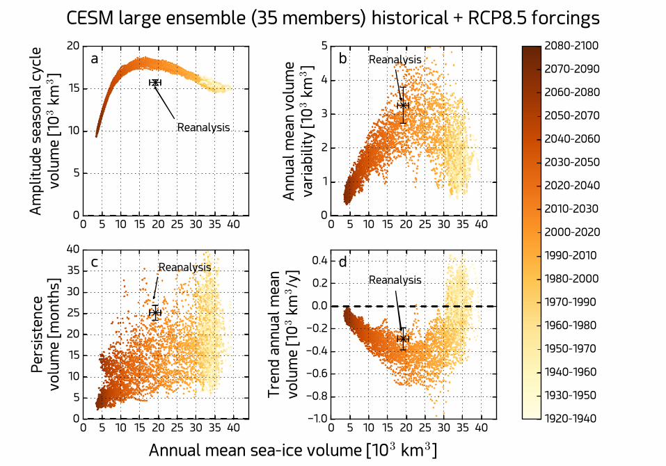
of growth and melt processes. Analyses conducted with the CESM-LE reveal that this
dependence indeed occurs in this model (Fig. 3). According to this GCM and a sea-ice
reanalysis22
, Arctic sea-ice volume has already experienced its most negative trends and
largest year-to-year variability. As the ice thins further, sea-ice volume will become less
persistent and exhibit less variability from one year to another. This contrasts with the
projected increases in summer sea-ice area variability and predictability, both regionally and
Arctic-wide23,24
.
The existence of relationships between the mean state and the efficiency of thermodynamic
processes, on the one hand, and between this efficiency and sea-ice area and volume
variability, on the other hand, allows to physically reinterpret the tight link that had been
noticed in earlier studies between mean state, seasonality, persistence, variability and
trends9,24,25
and seen in this study (Fig. 3). It also has an important implication: the confidence
in near-term predictions or long-term projections from models with a biased mean state
should be questioned. Indeed, linear post-processing methods widely used in the literature11,26
appear no longer justified since growth and melt efficiency, and hence sea-ice area and
volume variability, changes with the mean state. For the same reasons, weighted linear
Page 6
combination of model outputs27
have certainly statistical value but little physical basis. Based
on our findings, sea-ice projections obtained from simulations that have Arctic sea-ice volume
outside the observational range should be discarded as those simulations will not simulate
future thermodynamic sea-ice thinning correctly. Importantly, this does not mean that GCMs
with correct mean states are necessarily trustful for the future. Indeed, a failure to simulate
other, non-thermodynamic processes (e.g., sea-ice dynamics) may imply unreliable projected
sea-ice loss too. In addition, the current spatial distribution of sea-ice thickness28
or the
sensitivity of sea-ice extent to near-surface air temperatures29
are known critical factors
driving the future evolution of the sea-ice cover.
Given the importance of the mean state for ice-volume trends as highlighted in this study, a
natural final step would be to apply an observational constraint on the simulated volume
projections. However, estimating reliably the annual mean sea-ice volume directly from
observations is challenging, due to the short period for which large-scale estimates of sea-ice
thickness are available (~15 years). In addition, sea-ice thickness estimates are highly
uncertain not only because of instrumental errors, but also because of the numerous
assumptions on geophysical parameters (snow load, seawater, sea-ice and snow densities)
used to retrieve the actual thickness from the raw measurements30
. Following a highly
conservative methodology that takes these observational uncertainties into account (see
Methods), we come to the conclusion that it is currently not possible to significantly reduce
the spread in projected Arctic sea-ice volume loss (Fig. 4) due to too uncertain observations.
Reducing uncertainties in sea-ice area trend with the same constraint on sea-ice volume
appears to be even more challenging, as future trends in sea-ice area are subject to high
internal variability7. Thus, in line with the analyses presented in this study, the current main
obstacle to reducing uncertainties in projected sea-ice volume or area trends is not the
complexity of the models used, but rather the lack of long-term and reliable estimates of sea-
ice volume that can be used to constrain their projections.
Page 7
MAIN REFERENCES
1. IPCC, Climate Change 2013: The Physical Science Basis, Contribution of Working
Group I to the Fifth Assessment Report of the Intergovernmental Panel on Climate
Change, Cambridge Univ. Press, Cambridge (2013)
2. Stroeve, J., Kattsov, V., Barrett, A. P., Serreze, M., Pavlova, T., Holland, M., &
Meier, W.Trends in Arctic sea ice extent from CMIP5, CMIP3 and observations.
Geophys. Res. Lett.39, L16502 (2012)
3. Massonnet, F., Fichefet, T., Goosse, H., Bitz, C. M., Philippon-Berthier, G., Holland,
M. M., & Barriat, P. Y. Constraining projections of summer Arctic sea ice.
Cryosphere, 6, 1383–1394 (2012)
4. Wang, M., & Overland, J. E. A sea ice free summer Arctic within 30 years: An update
from CMIP5 models. Geophys. Res. Lett. 39, L1850 (2012)
5. Rosenblum, E., & Eisenman, I. Sea ice trends in climate models only accurate in runs
with biased global warming. J. Climate. 30, 6265–6278 (2017)
6. Mahlstein, I., & Knutti, R. Ocean heat transport as a cause for model uncertainty in
projected arctic warming. J. Climate, 24 1451–1460 (2011)
7. Notz, D. How well must climate models agree with observations? Phil. Trans. Roy.
Soc. A 373, 2052 (2014)
8. Holland, M. M., Bitz, C. M. & Tremblay, B. Future abrupt reductions in the summer
Arctic sea ice. Geophys. Res. Lett. 33, L23503 (2006)
9. Bitz, C. M. & Roe, G. H. A mechanism for the high rate of sea ice thinning in the
Arctic Ocean. J. Clim. 17, 3623–3632 (2004)
10. Kwok, R. et al. Thinning and volume loss of the Arctic Ocean sea ice cover: 2003–
2008. J. Geophys. Res. 114, C07005 (2009)
11. Melia, N., Haines, K. & Hawkins, E. Improved Arctic sea ice thickness projections
using bias-corrected CMIP5 simulations. Cryosphere 9, 2237–2251 (2015)
12. Swart, N., Fyfe, J. C., Hawkins, E., Kay, J. E. & Jahn, A. Influence of internal
variability on Arctic sea-ice trends. Nature Clim. Change 5, 86–89 (2015)
13. Bintanja, R. & van der Linden, E. C. The changing seasonal climate in the Arctic. Sci.
Rep. 3, 1556 (2013)
14. Holland, M. M., Serreze, M. C. & Stroeve, J. The sea ice mass budget of the Arctic
and its future change as simulated by coupled climate models. Clim. Dyn. 34, 185
(2010)
Page 8
15. Notz, D. and Bitz, C. M. Sea ice in Earth system models. in Sea Ice (Thomas Ed),
John Wiley & Sons (2017)
16. Curry, J. A., Schramm, J. L. and Ebert, E. E. Sea Ice-Albedo Climate Feedback
Mechanism. J. Climate 8 240-247 (1995)
17. Kay, J.E., et al. The Community Earth System Model (CESM) Large Ensemble
Project: A Community Resource for Studying Climate Change in the Presence of
Internal Climate Variability. Bull. Amer. Meteor. Soc. 96, 1333–1349 (2015)
18. Barnhart, K. R., Miller, C. R., Overeem, I., & Kay, J. E. Mapping the future expansion
of Arctic open water. Nature Clim. Change 6, 280–285 (2016)
19. Wenzel, S., Cox, P. M., Eyring, V. and Friedlingstein, P. Projected land
photosynthesis constrained by changes in the seasonal cycle of atmospheric CO2.
Nature 538 499-501 (2016)
20. Hunke, E. Thickness sensitivities in the CICE sea ice model. Ocean Model. 34, 137-
149 (2010)
21. Notz, D. et al. Sea Ice Model Intercomparison Project (SIMIP): Understanding sea ice
through climate-model simulations. Geosci. Model Dev. 9 3427–3446 (2016)
22. Schweiger, A., Lindsay, R., Zhang, J., Steele, M., Stern, H. Uncertainty in modeled
Arctic sea ice volume. J. Geophys. Res.116, C00D06 (2011)
23. Cheng, W., E. Blanchard-Wrigglesworth, C. M. Bitz, C. Ladd, and P. J. Stabeno
(2016), Diagnostic sea ice predictability in the pan-Arctic and U.S. Arctic regional
seas. Geophys. Res. Lett. 43, 11,688–11,696 (2016)
24. Goosse, H., Arzel, O., Bitz, C. M., de Montety, A. and Vancoppenolle, M. Increased
variability of the Arctic summer ice extent in a warmer climate. Geophys. Res. Lett.
36, L23702 (2009)
25. Blanchard-Wrigglesworth, E. & Bitz, C. M. Characteristics of Arctic sea-ice
variability in GCMs. J. Clim. 27, 8244–8258 (2014)
26. Fučkar, N. S., Volpi, D., Guemas, V. & Doblas-Reyes, F. J. A posteriori adjustment of
near-term climate predictions: Accounting for the drift dependence on the initial
conditions, Geophys. Res. Lett. 41, 5200-5207 (2014)
27. Knutti, R. et al. A climate model projection weighting scheme accounting for
performance and interdependence. Geophys. Res. Lett 44, 1909–1918 (2017)
28. Stroeve, J., Barrett, A., Serreze, M., and Schweiger, A. Using records from submarine,
aircraft and satellites to evaluate climate model simulations of Arctic sea ice thickness.
Cryosphere 8, 1839–1854 (2014)
Page 9
29. Zhang, X. Sensitivity of Arctic Summer Sea Ice Coverage to Global Warming
Forcing: Toward Reducing Uncertainty in Arctic Climate Change Projections. Tellus
A 62, 220–227 (2010)
30. Zygmuntowksa, M., Rampal, P., Ivanova, N., & Smedsrud, L. H. Uncertainties in
Arctic sea ice thickness and volume : new estimates and implications for trends.
Cryosphere 8 705-720 (2014)
31. Fetterer, F., K. Knowles, Meier, W., Savoie, M. & Windnagel, A. K., updated daily.
Sea Ice Index, Version 2. [G02135]. Boulder, Colorado USA. NSIDC: National Snow
and Ice Data Center. doi: http://dx.doi.org/10.7265/N5736NV7 (2017)
32. van Vuuren, D. et al. The representative concentration pathways: an overview. Clim.
Change 109 5-31 (2011)
33. EUMETSAT Ocean and Sea Ice Satelitte Application Facility. Global sea ice
concentration reprocessing dataset 1978-2015 (v1.2, 2015), [Online]. Norwegian and
Danish Meteorological Institutes. Available from http://osisaf.met.no
Correspondence
Correspondence and requests for materials should be addressed to François Massonnet
([email protected] ).
Acknowledgments
The research leading to these results has received funding from the Belgian Fonds National de
la Recherche Scientifique (F.R.S.-FNRS), the European Commission’s Horizon 2020 projects
APPLICATE (GA 727862) and PRIMAVERA (GA 641727). We acknowledge the World
Climate Research Programme’s Working Group on Coupled Modelling, which is responsible
for CMIP, and we thank the climate modelling groups (listed in the supplement) for producing
and making available their model output. We acknowledge the CESM Large Ensemble
Community Project and supercomputing resources provided by NSF/CISL/Yellowstone for
access to the CESM-LE data. The authors thank C. M. Bitz and D. Notz for useful
discussions, and F. Kauker for providing the ITRP data. The authors thank M. M. Holland, E.
C. Hunke and one anonymous reviewer for the review of this manuscript.
Author contributions
F.M., M.V. and H.G. designed the science plan. All authors contributed to the design of the
study. F.M. assembled the data and wrote the manuscript.
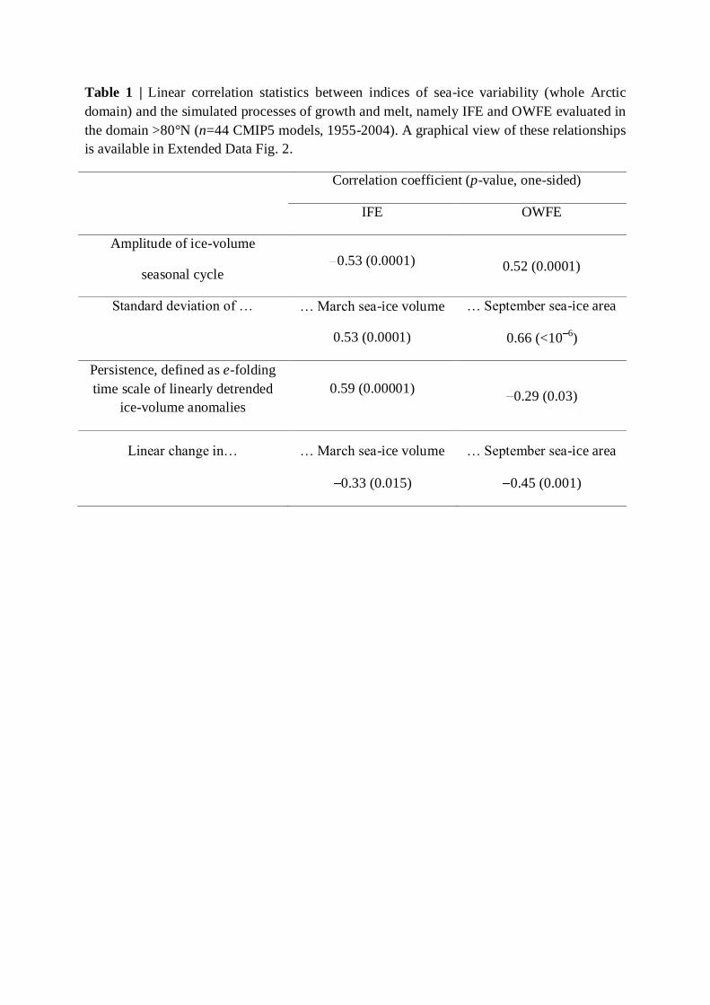
Page 10
Table 1 | Linear correlation statistics between indices of sea-ice variability (whole Arctic
domain) and the simulated processes of growth and melt, namely IFE and OWFE evaluated in
the domain >80°N (n=44 CMIP5 models, 1955-2004). A graphical view of these relationships
is available in Extended Data Fig. 2.
Correlation coefficient (p-value, one-sided)
IFE OWFE
Amplitude of ice-volume
seasonal cycle 0.53 (0.0001) 0.52 (0.0001)
Standard deviation of … … March sea-ice volume
0.53 (0.0001)
… September sea-ice area
0.66 (<106)
Persistence, defined as e-folding
time scale of linearly detrended
ice-volume anomalies
0.59 (0.00001) 0.29 (0.03)
Linear change in… … March sea-ice volume
0.33 (0.015)
… September sea-ice area
0.45 (0.001)
Page 11
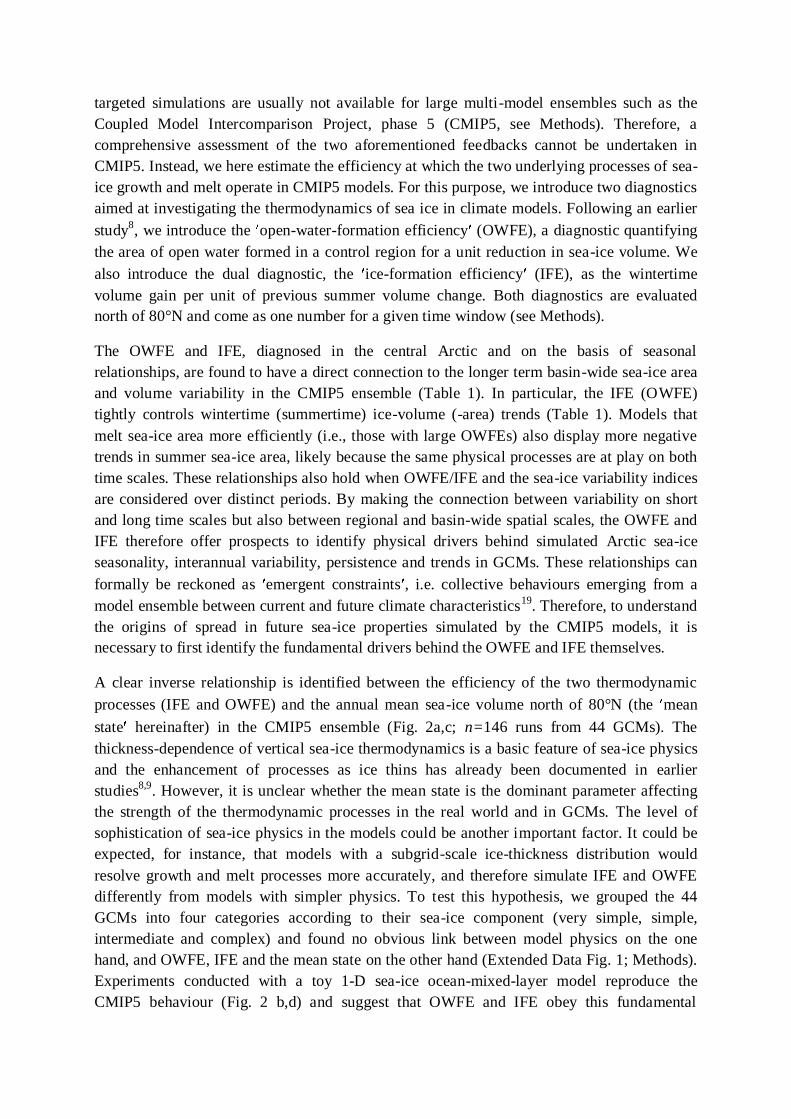
Figure 1 | Changing seasonality of Arctic sea-ice cover. a, Seasonal cycle of daily sea-ice extent
retrieved from satellite monitoring31, coloured by year (1979-2017). The bottom grey series indicates the
range (max-min) of sea-ice extent for each day of the year, after linear detrending of the data to remove
a first-order estimate of secular trends. b-c Average open-water seasonal formation for past (1850-1880)
and future (2020-2050) conditions estimated from the CESM-LE17 forced under historical and then
Representative Concentration Pathway32 (RCP) 8.5 forcings. Open-water seasonal formation is defined
for each calendar year, and each grid cell, as the range (max min) in sea-ice concentration for that year
and that grid cell. d-e Average sea-ice thickness seasonal change for the same past and future periods as
in b-c, using the same model outputs. Sea-ice thickness seasonal change is defined for each calendar
year and each grid cell as the range (max-min) of sea-ice thickness between July 1st and June 30st of the
next year. Light-pink contour lines denote the 15% contour line of September sea-ice concentration
averaged over the two reference periods.
Page 12
Figure 2 | Efficiency of growth and melt processes as a function of the mean state. a, Ice-
formation efficiency (IFE, see Methods) estimated from 44 CMIP5 models and their members
(n=146) over 1955-2004, plotted against the mean state defined as the annual mean sea-ice volume
north of 80°N averaged over the same period. Individual model realisations are plotted as dots and
ensemble means as circles; the size of circles is proportional to the number of members used for
averaging. A full referencing of CMIP5 models is available in Extended Data Table 1. Also plotted
are estimates from a sea-ice reanalysis22 (1979-2015) and from satellite retrievals10,33 (2003-2008).
Error bars on both estimates are the standard deviation on the corresponding diagnostics and mean
state (see Methods). b, IFE against mean state estimated from a 1-D sea-ice–ocean-mixed-layer
model (see Methods) integrated under reference conditions (black dot) and with varying sea-ice
conductivity, albedo and forcing (blue, green and red dots, respectively). The grey envelopes are the
one and two standard deviation confidence intervals from a 1/x fit of the CMIP5 data presented in a.
c, same as a but for the open-water-formation efficiency (OWFE). d, same as b but for the OWFE.
Page 13
Figure 3 | Influence of mean state on sea-ice volume variability. Relationship between four
indices of total Arctic sea-ice-volume variability (y-axes) and the mean state (annual mean Arctic
sea-ice volume north of 80°N) (x-axes) in a 35-member model ensemble (CESM-LE17) integrated
under historical and then RCP8.5 forcings32. The analysis is conducted on sliding 20-yr windows
(colour shading). a, Mean amplitude of the seasonal cycle; b, standard deviation of annual mean
sea-ice volume; c, persistence, estimated as the e-folding time scale of linearly detrended anomalies
of sea-ice volume; d, linear trend in annual mean sea-ice volume. Black crosses and error bars (see
Methods) correspond to the estimated mean state and variability from a sea-ice reanalysis22.
Page 14
Figure 4 | Challenges in reducing uncertainties of sea-ice volume projections. Time series of
annual mean Arctic sea-ice volume from historical and RCP8.5 forcings32 (72 simulations
available). Colours are referenced in Extended Table 1. Grey time series correspond to simulations
with sea-ice volume north of 80°N deemed incompatible with three observational references (see
Methods). The statistics reported at the top of the figure refer to the ensemble mean and standard
deviation of annual mean sea-ice volume linear change over 2020-2050 (for the full set of models,
“ALL”; and for the subset, “SUB”).
Page 15
METHODS
Data Availability.
All the results produced in this manuscript can be reproduced bit wise. The scripts used for
creating figures and statistics are available through the following public Github repository:
https://github.com/fmassonn/paper-arctic-processes
Specifically, the two functions evaluating the IFE and OWFE will be incorporated in the
Earth System Evaluation tool (ESMValTool, http://esmvaltool.org) for wider use by the
climate community.
The data used in the scripts above can be retrieved from the following archive:
https://doi.pangaea.de/10.1594/PANGAEA.889757
Instructions on how to use this data and how to run the scripts can be found in the
README.md file coming with the Github project above.
Domain of study for investigation of sea-ice thermodynamics. The goal of the present
study is to investigate how vertical thermodynamic processes affect the Arctic sea-ice volume
variability. The spatial domain must therefore be chosen appropriately in order to minimise
the effect of sea-ice dynamics on the results. A recent study25
has shown that thickness
variability at the local scale is largely dynamically driven. Conducting analyses at the model-
grid-cell level is therefore futile to measure thermodynamic processes. In contrast, a global
domain (such as the whole Arctic) is not desirable either, as sea-ice volume and area would be
impacted by horizontal oceanic processes which are not in the scope of our analyses. We
chose the oceanic cap north of 80°N as reference domain for five reasons: (1) the domain is
large enough to smooth out the effect of sea-ice dynamics on the area and thickness budgets,
(2) it is located in the interior of the multiyear ice zone during the historical period (1861-
2004) and therefore relatively sheltered from heat advected by the ocean from the south, (3)
the domain retains sea ice (even in summer) in most CMIP5 models until at least the mid-
century, while sea ice disappears seasonally elsewhere, (4) the domain is relatively well
sampled in terms of observations of sea-ice thickness (ICESat campaign10
), and (5) sensitivity
tests conducted a posteriori with a 1-D thermodynamic sea-ice ocean model (Fig. 2b, d)
reveal a remarkable similarity in the efficiency of processes as a function of the mean state.
This is of course not sufficient to claim that the choice of the domain is appropriate, but
indicates that the first-order thermodynamics of sea-ice models can be investigated in that
domain with reasonable confidence.
CMIP5 simulations.
Climate models. We analysed results from 44 GCMs participating to the Coupled Model
Intercomparison Project, phase 5 (CMIP5)34
, a suite of state-of-the-art climate models used as
scientific support for, e.g., the last International Panel on Climate Change report (IPCC
AR5)1. The number of 44 models corresponds to all models for which monthly mean outputs
Page 16
of sea-ice volume per unit grid-cell area (variable “sit”) and sea-ice concentration (variable
“sic”) were available over the historical period (1861-2004). Each model provides from one to
ten runs ( members ) that aim at sampling the intrinsic internal variability of the climate
system. We ran the diagnostics of the study for each member separately, but also presented
for convenience the ensemble mean of those diagnostics for each model. The statistics
reported, such as correlations, were always evaluated on the ensemble mean of diagnostics.
Sea-ice component in the models. Up to a few exceptions, nearly all climate models
participating to CMIP5 have a similar sea-ice dynamical component, based on the so-called
viscous-plastic rheology. The thermodynamic component of the models is more dependent on
the model, with some models explicitly simulating the subgrid-scale ice-thickness distribution
(ITD) and resolving heat conduction using multiple layers of ice and snow, while others
assume that sea ice can be represented as a slab with no thermal inertia. A clustering of the 44
CMIP5 models used in this study was done based on the documentation found in the literature
about the sea-ice components of those 44 models. Four groups were defined based on the
complexity of their sea-ice component: (1) very simple models, i.e. those without any
representation (explicit or implicit) of the subgrid-scale ITD (2) simple models, i.e. those
with an implicit (virtual) ITD, that is, in which conductive heat fluxes are corrected for the
unresolved nonlinear effects of the subgrid-scale ITD on vertical heat conduction fluxes, but
with no assumed heat capacity for sea ice (the so-called “0-layer” thermodynamics) (3)
intermediate models, i.e. those with either an explicit ITD but following the 0-layer
formalism, or with a virtual ITD but multiple layers of ice and snow, and (4) complex
models, i.e. those with an ITD and resolved multiple ice and snow layers. The correspondence
between the model name and model complexity is given in Extended Data Table 1.
CESM-LE simulations. Due to the limited number of members available from CMIP5
models (maximum 10), we ran additional analyses with the Community Earth System Model
Large Ensemble (CESM-LE)17
data set. This ensemble consists of n = 35 members integrated
from 1920 to 2100 under historical (1920-2005) and Representative Concentration Pathway32
(RCP) 8.5 (2006-2100) forcings. Similarly to CMIP5 models, the diagnostics were computed
on monthly mean outputs of sea-ice thickness and concentration, on the native grid of the
model. An overview of the ability of the CESM-LE to replicate observations is available in
Extended Data Fig. 3 (to be compared with Fig. 1a of the main manuscript).
Observational and reanalysis data. Daily values of Arctic sea-ice extent (Fig. 1a) are
retrieved from the National Snow and Ice Data Center (NSIDC) sea-ice index31
. Observed
sea-ice concentrations used for the evaluation of the Ice Formation Efficiency (IFE) and Open
Water Formation Efficiency (OWFE) (Fig. 2c) are retrieved from the Ocean and Sea Ice
Satellite Application Facility (OSI SAF) archive33
. Observed sea-ice thicknesses from the
ICESat satellite campaign10
are used for the evaluation of the two diagnostics (Fig. 2a-c).
Caution must be placed in the interpretation of the two diagnostics derived from observations,
as the reference period used to compute them is short (2003-2008) and the products
themselves are uncertain, particularly for sea-ice thickness. However, these products give a
first indication on the observed diagnostics and the resulting model biases. A sea-ice
reanalysis (PIOMAS)22
was also analysed. It consists of a 1979-2015 integration of an
Page 17
ocean sea-ice model nudged towards observed sea-ice concentrations and sea-surface
temperatures. Although being first and foremost a product derived from model outputs, this
reanalysis shows reasonable agreement with independent data22
.
1-D sea-ice ocean model. A one-dimensional thermodynamic sea-ice ocean-mixed-layer
model has been implemented to interpret physically the results obtained by GCMs. The code
of that toy model is available as Supplementary Information (see Long-term availability and
reproducibility of the results hereunder). The interpretation of results obtained from this
model should be made with caution, since this model lacks a number of processes and does
not display spatial dimensions. The physics of the model is a simplified and one-dimensional
version of the thermodynamic component of the Louvain-la-Neuve sea ice model, LIM235
.
Unlike LIM2, the toy model does not account for the thermal inertia of the ice, nor simulates
ice dynamics nor snow processes.
Model. The model has four state variables: sea-ice volume per grid cell area, sea-ice
concentration, sea-ice-surface temperature and ocean-mixed-layer temperature. No snow is
present at the top of sea ice. At each time step, an energy budget is computed at the open
ocean surface, and the heat imbalance is used to warm or cool a constant 30 m deep oceanic
mixed layer. We recognise the limitations behind this assumption, as in reality mixed-layer
depth exhibits seasonal variations36
. If the updated oceanic mixed-layer temperature drops
below the seawater freezing point ( 1.8°C), the equivalent energy is used to grow pure sea ice
(0 PSU) in open water (volumetric latent heat of fusion: 300.33 106 J/m
3), with an initial
thickness of 10 cm. This newly formed ice is accreted to the existing ice from the previous
time step. Then, an energy budget is computed at the top and bottom sea-ice surfaces to
determine how surface and basal processes modify sea-ice thickness and concentration. The
heat conductive flux through sea ice is derived from Fourier’s law assuming a constant sea-ice
thermal conductivity (2.0344 W/mK) and constant bottom ice temperature ( 1.8°C). The
conductive heat flux is boosted to account for the subgrid-scale variations in sea-ice thickness,
assuming that it is uniformly distributed between 0 m and twice the mean thickness37
. If the
net energy balance at the sea-ice top surface is positive, sea-ice thickness is reduced uniformly
assuming again that it is uniformly distributed between 0 and twice the mean value; this
results in a decrease in sea-ice concentration. An energy budget is finally computed at the
base of the ice. Here, a parameterised ocean-ice turbulent heat flux37
is used assuming
constant sea-ice velocity (1 cm/s), seawater density (1024.458 kg/m3) and drag coefficient
(0.005). The energy imbalance is used to grow or melt ice at the base of the existing ice floe.
Forcing. The atmospheric forcing used to drive the ice-ocean model follows the formulation
of Notz, 200538
based on the tabulated data of Maykut and Untersteiner, 197139
and Perovich
et al., 199940
. Incoming heat fluxes consist of a short-wave component and a non-solar
component. Sea-ice albedo varies throughout the year and is based on observational data. The
incoming fluxes are perturbed to emulate the interannual evolving nature of the atmosphere.
Reference experiment. In the standard case, the model is initialized from a 1.0-m-thick sea-ice
cover occupying 50% of the grid cell. Sea-ice-surface temperature is set to 10.0 °C and the
oceanic mixed-layer temperature is set to 1.8°C. The time step is one day. Under these
Page 18
conditions, the model reaches its equilibrium after ~15 years (Extended Data Fig. 4). The
equilibrium annual mean ice thickness (~3.5 m) corresponds, when integrated over the
domain north of 80°N (surface: 3.87 106
km2), to the volume of ~13.6 10
3 km
3 marked by
the black dot in Fig. 2b-d.
Sensitivity experiments. To produce the sensitivity experiments presented in Fig. 2b,d, we
integrated the model under various changes in parameters and forcings for 100 years and
conducted the analyses on the last 50 years of the simulations. We first incremented the sea-
ice thermal conductivity by 10, 20, 30, 40 and 50%, and then decreased it by the same
amounts (blue dots in Fig. 2b,d). Then we incremented the annual mean sea-ice albedo by 1,
2, 3, 4 and 5%, and decreased it by the same amounts (we kept the ice thermal conductivity at
its reference value). These are the green dots in Fig. 2b,d. Finally, we increased the annual
mean value of the non-solar forcing by 1, 2, 3, 4 and 5%, and decreased it by the same
amounts (we kept both the ice thermal conductivity and the annual mean sea-ice albedo at
their reference values). These are the red dots in Fig. 2b,d.
The IFE and OWFE diagnostics.
The evaluation of growth and melt processes require as input the time series of Arctic sea-ice
volume north of 80°N (for IFE) and sea-ice volume and area north of 80°N (for OWFE). The
original time series of volume and area from all 44 CMIP5 models are available in Extended
Data Figs. 5 and 6.
Ice-formation efficiency (IFE). The evaluation of the IFE is graphically illustrated in Extended
Data Fig. 7 (a,b). First, the time series of the Arctic sea-ice volume north of 80°N (see
Domain for investigation of sea-ice thermodynamics above) is computed. Then, for each
calendar year of the time series but the last one, (1) the annual minimum sea-ice volume is
recorded for that year (Vmin) and (2) the annual maximum of the next year is recorded (Vmax).
The ice volume created ( V=Vmax Vmin) is then computed. Finally, a linear regression is
conducted between Vmin (x, predictor) and V (y, predictand) over all years. The IFE is
defined as the slope of the regression line between V and Vmin. By default, both V and Vmin
are linearly detrended prior to the regression in order to avoid spurious relationships between
those variables due to possible secular trends. This detrending does not affect the conclusions
of the manuscript (Extended Data Fig. 8a).
The IFE is a dimensionless number and can be interpreted as the efficiency of a model to
recover a summer anomaly of sea-ice volume either completely (IFE = 1.0) or not at all (IFE
= 0.0).
Extended Data Fig. 9 illustrates the methodology for all 44 CMIP5 models.
Open-water-formation Efficiency (OWFE). The diagnostic derives from from Holland et al.,
20068. The evaluation of the OWFE is graphically illustrated in Extended Data Fig. 7 (c,d).
First, the time series of the Arctic sea-ice volume and area north of 80°N (see ‘Domain for
investigation of sea-ice thermodynamics’ above) are computed. Then, for each calendar year
of the time series, the months of annual maximum and minimum sea-ice volumes are recorded
Page 19
(tmin and tmax, respectively). The volume loss for that year V =V(tmin) V(tmax) is estimated.
The area loss for that year A =A(tmin) A(tmax) is computed. Note that the area difference is
not taken between the minimum and maximum of area time series, which do not necessarily
coincide with the timings of volume extrema. Finally, a linear regression is conducted
between V (x, predictor) and A (y, predictand) over all years. The OWFE is defined as the
slope of the regression line between A and V. By default, both A and V are linearly
detrended prior to the regression to avoid spurious relationships between those variables due
to secular trends. This detrending does not affect the conclusions of the manuscript (Extended
Data Fig. 8b).
The OWFE is a number with units m-1
and measures the efficiency at which a model forms
open water (or reduces sea-ice area) given a unit reduction in sea-ice thickness8.
Extended Data Fig. 10 illustrates the methodology for all 44 CMIP5 models.
Physical meaning. It is important to recognise that neither OWFE nor IFE are strict measures
of feedback per se. However, since both melt and growth processes are central elements in the
negative and positive feedback loops described above, the two diagnostics allow appreciating
the first-order role played by sea ice in these feedbacks.
Uncertainty. Both IFE and OWFE are defined as regression coefficients. The standard
deviation of the estimated coefficients is taken as the measure of uncertainty on the two
diagnostics (e.g., for observations and the reanalysis in Fig. 2). The uncertainty in annual
mean sea-ice volume is defined as the standard deviation of annual mean sea-ice volume time
series (e.g., Figs. 2 and 3).
No sensitivity to reference period. The analyses with CMIP5 models are conducted over the
reference period 1955-2004, which corresponds to the last 50 years of the historical period
defined by the CMIP5 protocol34
. The robustness of the findings was tested using different
periods. Results were found to be insensitive to this choice (Extended Data Fig. 11). Results
were also found to be robust with respect to the separation in time: computation of OWFE and
IFE on an earlier period than the Arctic sea-ice variability indices yields similar results
(Extended Data Fig. 12).
Can we reduce uncertainties in projected ice-volume trends?
Bitz and Roe (2004)9
first identified a robust relationship between the simulated Arctic annual
mean sea-ice volume and the projected volume loss. In line with their conclusions and with
the physical arguments given in our manuscript, we also reproduce this result (Extended Data
Fig. 13). From this relationship, it would appear natural to subset the CMIP5 ensemble based
on their ability to simulate the observed annual mean sea-ice volume in our domain of study
(i.e., the x-axis of Extended Data Fig. 15). However, there are at least four obstacles that make
the application of this constraint difficult: (1) there is considerable uncertainty in the raw
retrievals in observations of ice freeboard and draft due to instrumental error, (2) there is
considerable uncertainty in the deduced sea-ice thickness due to assumptions (e.g., hydrostatic
equilibrium, climatological snow load) and the parameters used to convert the raw
Page 20
measurements to sea-ice thickness (snow and ice density are taken as constants)30
, (3) the
period for which large-scale estimates of sea-ice volume are available is short (~15 years) and
interannual variability is large, meaning that time averages are subject to large sampling
errors, and (4) sea-ice thickness uncertainties are particularly large (or no sea-ice thickness
estimates are available) in summer. Given all these sources of uncertainty, it appears clearly
that reliably estimating the true annual mean sea-ice volume from observations is impossible
nowadays, and hence applying a reliable constraint based on the annual mean sea ice volume
is not feasible.
As an alternative, we follow a much less constrained approach. We discard simulations that
have a monthly mean sea-ice volume north of 80°N systematically higher or lower than three
standard observational references: IceSat, CryoSat2 and the ITRP datasets10,41,42
over the
period of observational data availability (2000-2017, Extended Data Fig. 14). In other words,
we disregard simulations for which the sea-ice volume north of 80°N for each month of each
year is always outside the observational range. Applying this constraint on the CMIP5
ensemble (RCP8.5, 2005-2100), we discard 14 simulations out of 72 available. The ensemble
mean of 2020-2050 projected ice-volume loss hardly changes after the application of this
constraint (from 6.85 to 6.80 103 km
3) and the spread around these estimates is only
reduced by about 17% (from 3.08 to 2.56 103 km
3) (Fig. 4).
METHODS-ONLY REFERENCES
34. Taylor, K. E., Stouffer, R. J., Meehl, G. A. An overview of CMIP5 and the experiment
design. Bull. Am. Meteorol. Soc. 93 485–498 (2012)
35. Fichefet, T. & Morales Maqueda, M. M. Sensitivity of a global sea ice model to the
treatment of ice thermodynamics and dynamics. J. Geophys. Res. 102 C6 12609–
12646 (1997)
36. Tsamados, M., Feltham, D., Petty, A., Schroeder, D. & Flocco, D. Processes
controlling surface, bottom and lateral melt of Arctic sea ice in a state of the art sea ice
model. Phil. Trans. Roy. Soc. A 373, 2052 (2015)
37. Goosse, H. & Fichefet, T. Importance of ice-ocean interactions for the global ocean
circulation: A model study. J. Geophys. Res. 104 23337–23335 (1999)
38. Notz, D. Thermodynamic and fluid-dynamical processes in sea ice. Ph.D. thesis,
University of Cambridge (2005)
39. Maykut, G. A. and Untersteiner, N. Some results from a time–dependent,
thermodynamic model of sea ice. J. Geophys. Res., 76 1550–1575 (1971)
40. Perovich, D. K., Grenfell T. C., Light B., Richter-Menge, J. A., Sturm M., Tucker III,
W. V., Eicken, H., Maykut, G. A. and Elder, B. SHEBA: Snow and Ice Studies CD-
ROM. Technical report, Cold Regions Research and Engineering Laboratory (1999)
Page 21
41. Hendricks, S., Ricker, R. and Helm, V. AWI CryoSat-2 Sea Ice Thickness Data
Product (v1.2), User Guide.
http://www.meereisportal.de/fileadmin/user_upload/www.meereisportal.de/MeereisBe
obachtung/Beobachtungsergebnisse_aus_Satellitenmessungen/CryoSat-
2_Meereisprodukt/AWI_cryosat2_user_guide_v1.2_july2016.pdf (2016)
42. Lindsay, R. and Schweiger, A. Arctic sea ice thicknes loss determined using
subsurface, aircraft, and satellite observations. Cryosphere 9, 269-283 (2015)
Page 22
Jan Feb Mar Apr May Jun Jul Aug Sep Oct Nov Dec0
2
4
6
8
10
12
14
16
106 k
m2
Range (trend removed)
aObserved Arctic sea-ice extent, 1979-2017
b
Open water formed1850-1880 (model)
c
Open water formed2020-2050 (model)
d
Ice thickness seasonalchange 1850-1880 (model)
e
Ice thickness seasonalchange 2020-2050 (model)
1980 1985 1990 1995 2000 2005 2010 2015
0
20
40
60
80
100
0
20
40
60
80
100
%
0.0
0.5
1.0
1.5
2.0
2.5
0.0
0.5
1.0
1.5
2.0
2.5
m
Page 23
0 5 10 15 20 251.0
0.8
0.6
0.4
0.2
0.0
0.2IF
E [m
/m]
0102
03
04
0506
07
080910
11
12
1314
15
1617
18
19
2021
22
2324
25
26
27
28
29
30
31
32
3334
35
36
37
38
39
40
4142
43 44
a
OBS
Reanalysis
44 CMIP5 models (146 members)
0 5 10 15 20 25Annual mean ice volume [103 km3]
0.2
0.0
0.2
0.4
0.6
0.8
1.0
OW
FE [m
−1]
0102
03
04
05
06
07
08
09
1011
121314
15
16
17
18
19
20
2122
23
24
25
26
27
28
29
30
31 32
33
34
35
3637
3839
40
4142
43
44
c
OBS
Reanalysis
0 5 10 15 20 251.0
0.8
0.6
0.4
0.2
0.0
0.2
CMIP5
b1-D thermodynamic model
0 5 10 15 20 25Annual mean ice volume [103 km3]
0.2
0.0
0.2
0.4
0.6
0.8
1.01-D model referenceice conductivity variedice albedo variedforcing varied
CMIP5
d
Page 24
0 5 10 15 20 25 30 35 400
5
10
15
20Am
plitu
de s
easo
nal c
ycle
volu
me
[10
3 k
m3]
Reanalysis
a
0 5 10 15 20 25 30 35 400
1
2
3
4
5
Annu
al m
ean
volu
me
vari
abili
ty [1
03 k
m3] Reanalysisb
0 5 10 15 20 25 30 35 400
5
10
15
20
25
30
35
40
Pers
iste
nce
volu
me
[mon
ths]
Reanalysisc
0 5 10 15 20 25 30 35 401.0
0.8
0.6
0.4
0.2
0.0
0.2
0.4Tr
end
annu
al m
ean
volu
me
[10
3 k
m3/y
]Reanalysis
d
1920-1940
1930-1950
1940-1960
1950-1970
1960-1980
1970-1990
1980-2000
1990-2010
2000-2020
2010-2030
2020-2040
2030-2050
2040-2060
2050-2070
2060-2080
2070-2090
2080-2100
Annual mean sea-ice volume [103 km3]
CESM large ensemble (35 members) historical + RCP8.5 forcings
Page 25
2000 2020 2040 2060 2080 21000
5
10
15
20
Annu
al m
ean
sea-
ice
volu
me
[10
3 k
m3]
2020-2050 ice-volume loss (>80N):ALL: -2.53 +/- 1.33 x 10³ km3
SUB: -2.64 +/- 1.24 x 10³ km3
72 CMIP5 simulations(historical + RCP8.5 scenarios)