Introduction Minimax Search Evaluation Fns Alpha-Beta Search MCTS Conclusion References Artificial Intelligence 6. Adversarial Search What To Do When Your “Solution” is Somebody Else’s Failure ´ Alvaro Torralba Wolfgang Wahlster Summer Term 2018 Thanks to Prof. Hoffmann for slide sources Torralba and Wahlster Artificial Intelligence Chapter 6: Adversarial Search 1/58
Playing a game well clearly requires a form of “intelligence”.
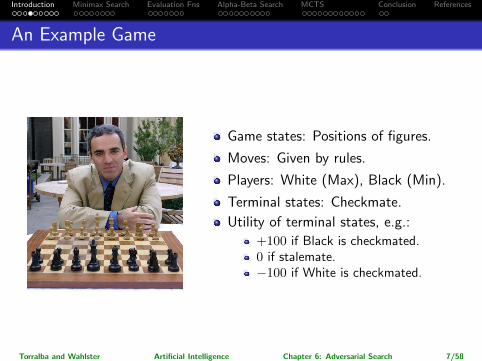
Games capture a pure form of competition between opponents.
Games are abstract and precisely defined, thus very easy toformalize.
→ Game playing is one of the oldest sub-areas of AI (ca. 1950).
→ The dream of a machine that plays Chess is, indeed, much older thanAI! (von Kempelen’s “Schachturke” (1769), Torres y Quevedo’s “ElAjedrecista” (1912))
Torralba and Wahlster Artificial Intelligence Chapter 6: Adversarial Search 5/58
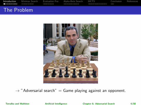
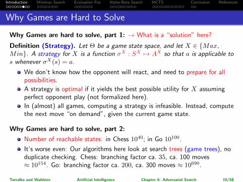
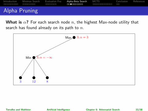
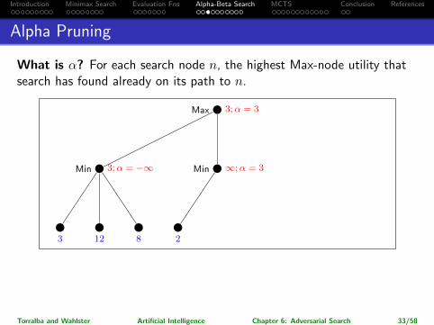
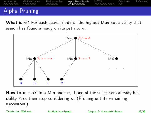
Why Games are hard to solve, part 1: → What is a “solution” here?
Definition (Strategy). Let Θ be a game state space, and let X ∈ {Max,Min}. A strategy for X is a function σX : SX 7→ AX so that a is applicable tos whenever σX(s) = a.
We don’t know how the opponent will react, and need to prepare for allpossibilities.
A strategy is optimal if it yields the best possible utility for X assumingperfect opponent play (not formalized here).
In (almost) all games, computing a strategy is infeasible. Instead, computethe next move “on demand”, given the current game state.
Why Games are hard to solve, part 2:
Number of reachable states: in Chess 1040; in Go 10100.
It’s worse even: Our algorithms here look at search trees (game trees), noduplicate checking. Chess: branching factor ca. 35, ca. 100 moves≈ 10154. Go: branching factor ca. 200, ca. 300 moves ≈ 10690.
Torralba and Wahlster Artificial Intelligence Chapter 6: Adversarial Search 10/58
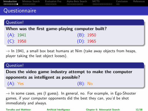
→ In 1941, a small box beat humans at Nim (take away objects from heaps,player taking the last object looses).
Question!
Does the video game industry attempt to make the computeropponents as intelligent as possible?
(A): Yes (B): No
→ In some cases, yes (I guess). In general, no. For example, in Ego-Shootergames, if your computer opponents did the best they can, you’d be shotimmediately and always.
Torralba and Wahlster Artificial Intelligence Chapter 6: Adversarial Search 12/58
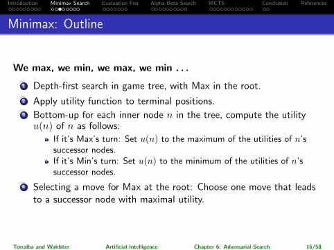
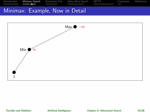
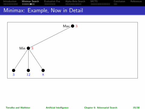
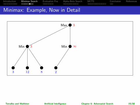
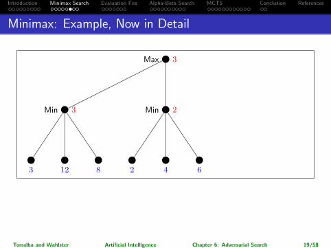
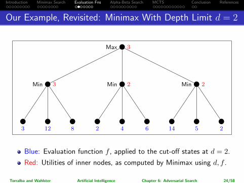
1 Depth-first search in game tree, with Max in the root.
2 Apply utility function to terminal positions.3 Bottom-up for each inner node n in the tree, compute the utilityu(n) of n as follows:
If it’s Max’s turn: Set u(n) to the maximum of the utilities of n’ssuccessor nodes.If it’s Min’s turn: Set u(n) to the minimum of the utilities of n’ssuccessor nodes.
4 Selecting a move for Max at the root: Choose one move that leadsto a successor node with maximal utility.
Torralba and Wahlster Artificial Intelligence Chapter 6: Adversarial Search 16/58
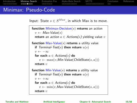
function Minimax-Decision(s) returns an actionv ← Max-Value(s)return an action a ∈ Actions(s) yielding value v
function Max-Value(s) returns a utility valueif Terminal-Test(s) then return u(s)v ← −∞for each a ∈ Actions(s) dov ← max(v,Min-Value(ChildState(s, a)))
return v
function Min-Value(s) returns a utility valueif Terminal-Test(s) then return u(s)v ← +∞for each a ∈ Actions(s) dov ← min(v,Max-Value(ChildState(s, a)))
return v
Torralba and Wahlster Artificial Intelligence Chapter 6: Adversarial Search 18/58
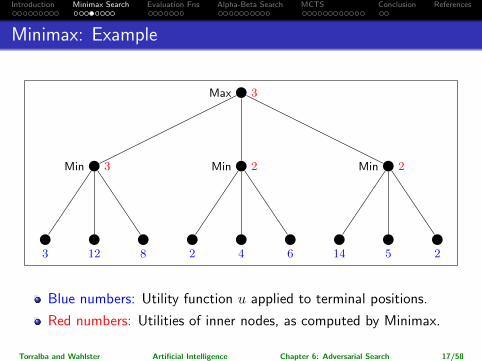
Note: The maximalpossible pay-off is higher for the rightmost branch, but assuming perfect play ofMin, it’s better to go left. (Going right would be “relying on your opponent todo something stupid”.)
Torralba and Wahlster Artificial Intelligence Chapter 6: Adversarial Search 19/58
Note: The maximalpossible pay-off is higher for the rightmost branch, but assuming perfect play ofMin, it’s better to go left. (Going right would be “relying on your opponent todo something stupid”.)
Torralba and Wahlster Artificial Intelligence Chapter 6: Adversarial Search 19/58
Note: The maximalpossible pay-off is higher for the rightmost branch, but assuming perfect play ofMin, it’s better to go left. (Going right would be “relying on your opponent todo something stupid”.)
Torralba and Wahlster Artificial Intelligence Chapter 6: Adversarial Search 19/58
Note: The maximalpossible pay-off is higher for the rightmost branch, but assuming perfect play ofMin, it’s better to go left. (Going right would be “relying on your opponent todo something stupid”.)
Torralba and Wahlster Artificial Intelligence Chapter 6: Adversarial Search 19/58
Note: The maximalpossible pay-off is higher for the rightmost branch, but assuming perfect play ofMin, it’s better to go left. (Going right would be “relying on your opponent todo something stupid”.)
Torralba and Wahlster Artificial Intelligence Chapter 6: Adversarial Search 19/58
Note: The maximalpossible pay-off is higher for the rightmost branch, but assuming perfect play ofMin, it’s better to go left. (Going right would be “relying on your opponent todo something stupid”.)
Torralba and Wahlster Artificial Intelligence Chapter 6: Adversarial Search 19/58
Note: The maximalpossible pay-off is higher for the rightmost branch, but assuming perfect play ofMin, it’s better to go left. (Going right would be “relying on your opponent todo something stupid”.)
Torralba and Wahlster Artificial Intelligence Chapter 6: Adversarial Search 19/58
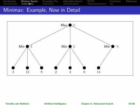
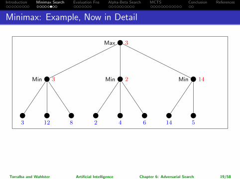
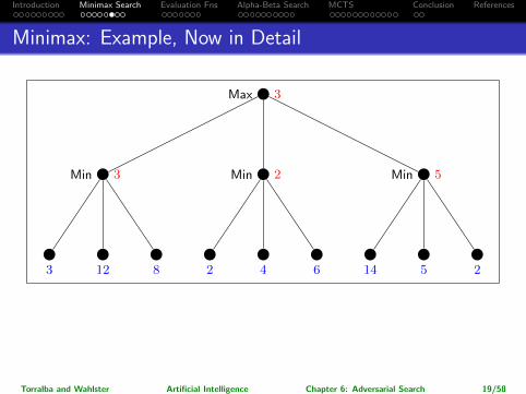
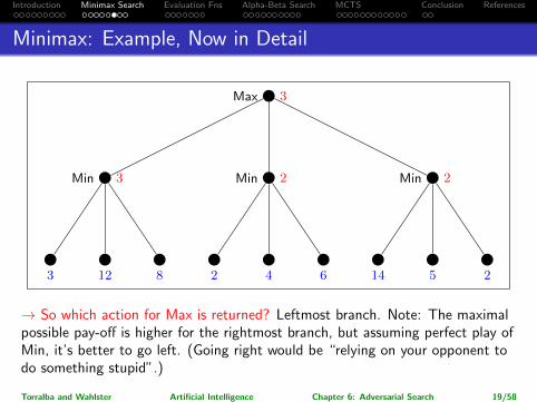
→ So which action for Max is returned? Leftmost branch. Note: The maximalpossible pay-off is higher for the rightmost branch, but assuming perfect play ofMin, it’s better to go left. (Going right would be “relying on your opponent todo something stupid”.)
Torralba and Wahlster Artificial Intelligence Chapter 6: Adversarial Search 19/58
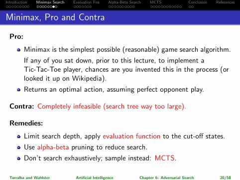
Minimax is the simplest possible (reasonable) game search algorithm.
If any of you sat down, prior to this lecture, to implement aTic-Tac-Toe player, chances are you invented this in the process (orlooked it up on Wikipedia).
Returns an optimal action, assuming perfect opponent play.
Contra: Completely infeasible (search tree way too large).
Remedies:
Limit search depth, apply evaluation function to the cut-off states.
Use alpha-beta pruning to reduce search.
Don’t search exhaustively; sample instead: MCTS.
Torralba and Wahlster Artificial Intelligence Chapter 6: Adversarial Search 20/58
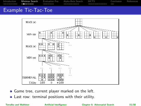
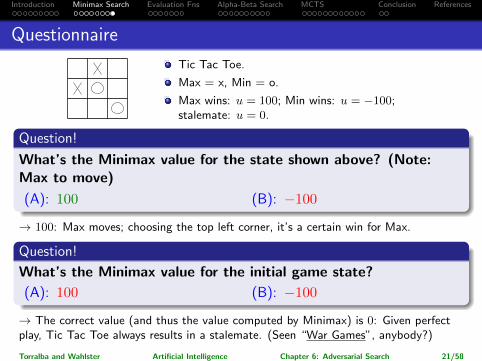
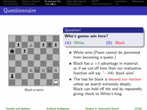
Max wins: u = 100; Min wins: u = −100;stalemate: u = 0.
Question!
What’s the Minimax value for the state shown above? (Note:Max to move)
(A): 100 (B): −100
→ 100: Max moves; choosing the top left corner, it’s a certain win for Max.
Question!
What’s the Minimax value for the initial game state?
(A): 100 (B): −100
→ The correct value (and thus the value computed by Minimax) is 0: Given perfectplay, Tic Tac Toe always results in a stalemate. (Seen “War Games”, anybody?)
Torralba and Wahlster Artificial Intelligence Chapter 6: Adversarial Search 21/58
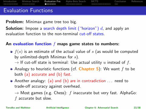
Solution: Impose a search depth limit (“horizon”) d, and apply anevaluation function to the non-terminal cut-off states.
An evaluation function f maps game states to numbers:
f(s) is an estimate of the actual value of s (as would be computedby unlimited-depth Minimax for s).→ If cut-off state is terminal: Use actual utility u instead of f .
Analogy to heuristic functions (cf. Chapter 5): We want f to beboth (a) accurate and (b) fast.
Another analogy: (a) and (b) are in contradiction . . . need totrade-off accuracy against overhead.
→ Most games (e.g. Chess): f inaccurate but very fast. AlphaGo:f accurate but slow.
Torralba and Wahlster Artificial Intelligence Chapter 6: Adversarial Search 23/58
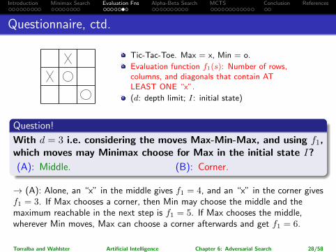
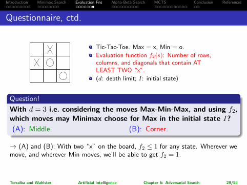
Evaluation function f1(s): Number of rows,columns, and diagonals that contain ATLEAST ONE “x”.
(d: depth limit; I: initial state)
Question!
With d = 3 i.e. considering the moves Max-Min-Max, and using f1,which moves may Minimax choose for Max in the initial state I?
(A): Middle. (B): Corner.
→ (A): Alone, an “x” in the middle gives f1 = 4, and an “x” in the corner givesf1 = 3. If Max chooses a corner, then Min may choose the middle and themaximum reachable in the next step is f1 = 5. If Max chooses the middle,wherever Min moves, Max can choose a corner afterwards and get f1 = 6.
Torralba and Wahlster Artificial Intelligence Chapter 6: Adversarial Search 28/58
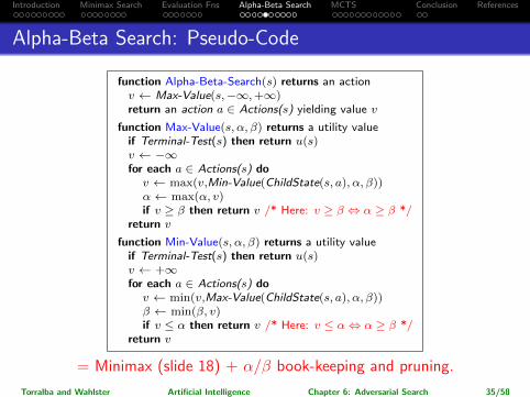
function Alpha-Beta-Search(s) returns an actionv ← Max-Value(s,−∞,+∞)return an action a ∈ Actions(s) yielding value v
function Max-Value(s, α, β) returns a utility valueif Terminal-Test(s) then return u(s)v ← −∞for each a ∈ Actions(s) dov ← max(v,Min-Value(ChildState(s, a), α, β))α ← max(α, v)if v ≥ β then return v /* Here: v ≥ β ⇔ α ≥ β */
return v
function Min-Value(s, α, β) returns a utility valueif Terminal-Test(s) then return u(s)v ← +∞for each a ∈ Actions(s) dov ← min(v,Max-Value(ChildState(s, a), α, β))β ← min(β, v)if v ≤ α then return v /* Here: v ≤ α⇔ α ≥ β */
return v
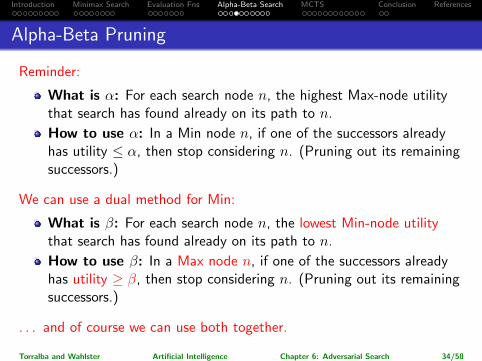
= Minimax (slide 18) + α/β book-keeping and pruning.
Torralba and Wahlster Artificial Intelligence Chapter 6: Adversarial Search 35/58
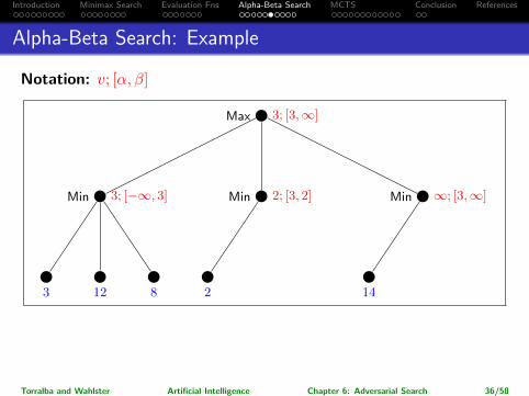
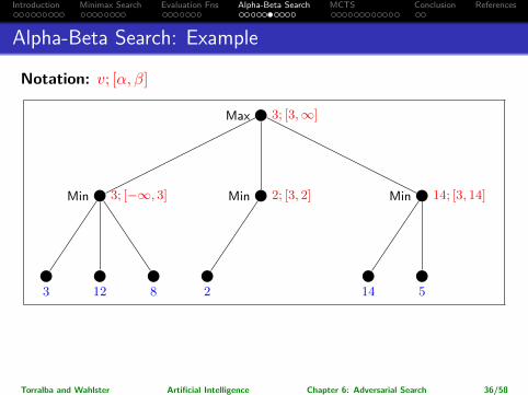
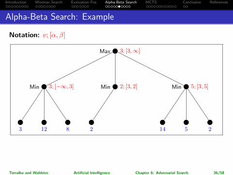
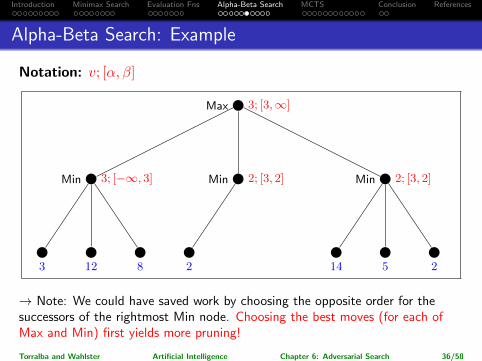
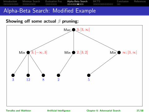
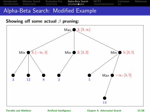
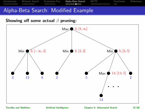
→ Note: We could have saved work by choosing the opposite order for thesuccessors of the rightmost Min node. Choosing the best moves (for each ofMax and Min) first yields more pruning!
Torralba and Wahlster Artificial Intelligence Chapter 6: Adversarial Search 36/58
→ Note: We could have saved work by choosing the opposite order for thesuccessors of the rightmost Min node. Choosing the best moves (for each ofMax and Min) first yields more pruning!
Torralba and Wahlster Artificial Intelligence Chapter 6: Adversarial Search 36/58
→ Note: We could have saved work by choosing the opposite order for thesuccessors of the rightmost Min node. Choosing the best moves (for each ofMax and Min) first yields more pruning!
Torralba and Wahlster Artificial Intelligence Chapter 6: Adversarial Search 36/58
→ Note: We could have saved work by choosing the opposite order for thesuccessors of the rightmost Min node. Choosing the best moves (for each ofMax and Min) first yields more pruning!
Torralba and Wahlster Artificial Intelligence Chapter 6: Adversarial Search 36/58
→ Note: We could have saved work by choosing the opposite order for thesuccessors of the rightmost Min node. Choosing the best moves (for each ofMax and Min) first yields more pruning!
Torralba and Wahlster Artificial Intelligence Chapter 6: Adversarial Search 36/58
→ Note: We could have saved work by choosing the opposite order for thesuccessors of the rightmost Min node. Choosing the best moves (for each ofMax and Min) first yields more pruning!
Torralba and Wahlster Artificial Intelligence Chapter 6: Adversarial Search 36/58
→ Note: We could have saved work by choosing the opposite order for thesuccessors of the rightmost Min node. Choosing the best moves (for each ofMax and Min) first yields more pruning!
Torralba and Wahlster Artificial Intelligence Chapter 6: Adversarial Search 36/58
→ Note: We could have saved work by choosing the opposite order for thesuccessors of the rightmost Min node. Choosing the best moves (for each ofMax and Min) first yields more pruning!
Torralba and Wahlster Artificial Intelligence Chapter 6: Adversarial Search 36/58
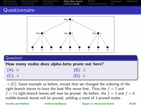
→ (C): Same example as before, except that we changed the ordering of theright-branch leaves to have the best Min move first. Thus the f = 5 andf = 14 right-branch leaves will now be pruned. As before, the f = 4 and f = 6middle-branch leaves will be pruned, yielding a total of 4 pruned nodes.
Torralba and Wahlster Artificial Intelligence Chapter 6: Adversarial Search 40/58
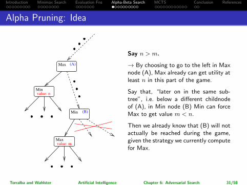
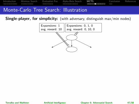
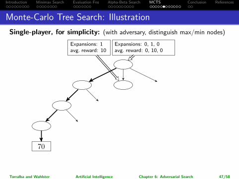
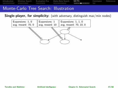
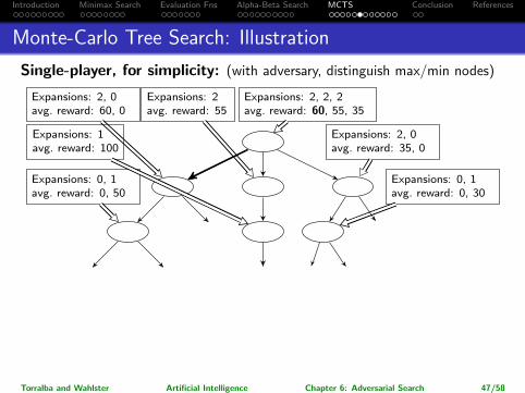
Alpha Beta search is a strong algorithm but it has two issues (e.g. in Go):
1 It needs an accurate/fast evaluation function. This is not alwayseasy to obtain. For example, traditionally there have not been verygood evaluation functions for the game of Go.
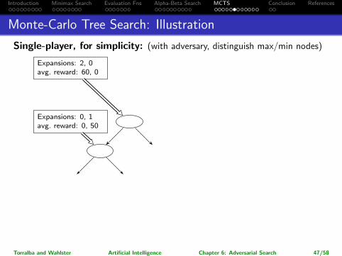
→Evaluate positions by playing random games.
f(s) = average utility of these simulations
2 Not so much exploration in problems with large branching factor.The branching factor in Go is ≈ 300 moves. To explore the full treeminimax tree up to depth 3, we need 3003 = 27.000.000 evaluations.
→Spent more time evaluating “promising” moves.
Torralba and Wahlster Artificial Intelligence Chapter 6: Adversarial Search 43/58
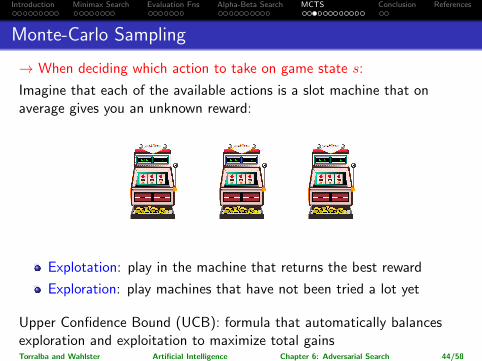
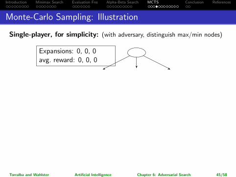
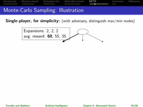
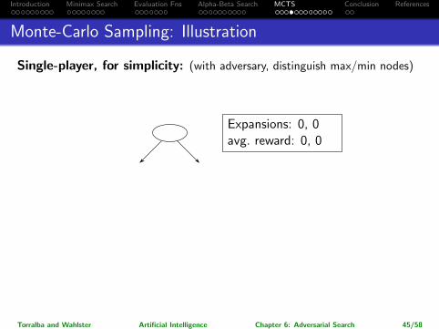
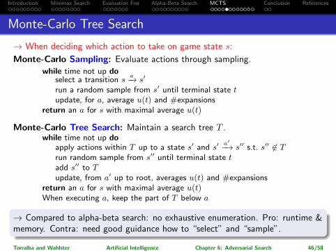
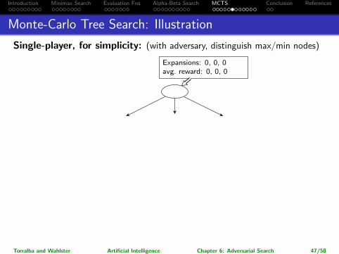
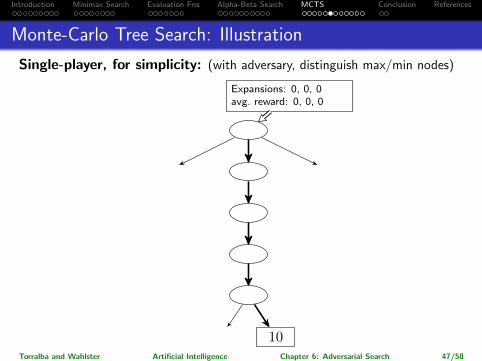
→ When deciding which action to take on game state s:
Imagine that each of the available actions is a slot machine that onaverage gives you an unknown reward:
Explotation: play in the machine that returns the best reward
Exploration: play machines that have not been tried a lot yet
Upper Confidence Bound (UCB): formula that automatically balancesexploration and exploitation to maximize total gainsTorralba and Wahlster Artificial Intelligence Chapter 6: Adversarial Search 44/58
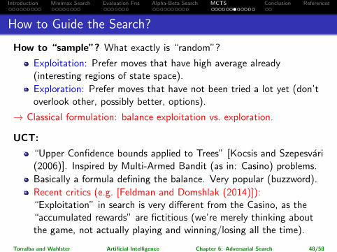
Exploitation: Prefer moves that have high average already(interesting regions of state space).
Exploration: Prefer moves that have not been tried a lot yet (don’toverlook other, possibly better, options).
→ Classical formulation: balance exploitation vs. exploration.
UCT:
“Upper Confidence bounds applied to Trees” [Kocsis and Szepesvari(2006)]. Inspired by Multi-Armed Bandit (as in: Casino) problems.
Basically a formula defining the balance. Very popular (buzzword).
Recent critics (e.g. [Feldman and Domshlak (2014)]):“Exploitation” in search is very different from the Casino, as the“accumulated rewards” are fictitious (we’re merely thinking aboutthe game, not actually playing and winning/losing all the time).
Torralba and Wahlster Artificial Intelligence Chapter 6: Adversarial Search 48/58
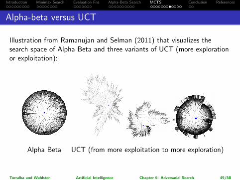
Illustration from Ramanujan and Selman (2011) that visualizes thesearch space of Alpha Beta and three variants of UCT (more explorationor exploitation):
Alpha Beta UCT (from more exploitation to more exploration)
Torralba and Wahlster Artificial Intelligence Chapter 6: Adversarial Search 49/58
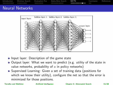
Input layer: Description of the game stateOutput layer: What we want to predict (e.g. utility of the state invalue networks, probability of a in policy networks)Supervised Learning: Given a set of training data (positions forwhich we know their utility), configure the net so that the error isminimized for those positions.
Torralba and Wahlster Artificial Intelligence Chapter 6: Adversarial Search 51/58
Games (2-player turn-taking zero-sum discrete and finite games) can beunderstood as a simple extension of classical search problems.
Each player tries to reach a terminal state with the best possible utility(maximal vs. minimal).
Minimax searches the game depth-first, max’ing and min’ing at therespective turns of each player. It yields perfect play, but takes time O(bd)where b is the branching factor and d the search depth.
Except in trivial games (Tic-Tac-Toe), Minimax needs a depth limit andapply an evaluation function to estimate the value of the cut-off states.
Alpha-beta search remembers the best values achieved for each playerelsewhere in the tree already, and prunes out sub-trees that won’t bereached in the game.
Monte-Carlo tree search (MCTS) samples game branches, and averagesthe findings. AlphaGo controls this using neural networks: evaluationfunction (“value network”), and action filter (“policy network”).
Torralba and Wahlster Artificial Intelligence Chapter 6: Adversarial Search 55/58
Content: Section 5.1 corresponds to my “Introduction”, Section 5.2corresponds to my “Minimax Search”, Section 5.3 corresponds tomy “Alpha-Beta Search”. I have tried to add some additionalclarifying illustrations. RN gives many complementary explanations,nice as additional background reading.
Section 5.4 corresponds to my “Evaluation Functions”, but discussesadditional aspects relating to narrowing the search and look-up fromopening/termination databases. Nice as additional backgroundreading.
I suppose a discussion of MCTS and AlphaGo will be added to thenext edition . . .
Torralba and Wahlster Artificial Intelligence Chapter 6: Adversarial Search 56/58
Zohar Feldman and Carmel Domshlak. Simple regret optimization in online planningfor markov decision processes. Journal of Artificial Intelligence Research,51:165–205, 2014.
Levente Kocsis and Csaba Szepesvari. Bandit based Monte-Carlo planning. InJohannes Furnkranz, Tobias Scheffer, and Myra Spiliopoulou, editors, Proceedingsof the 17th European Conference on Machine Learning (ECML 2006), volume 4212of Lecture Notes in Computer Science, pages 282–293. Springer-Verlag, 2006.
Raghuram Ramanujan and Bart Selman. Trade-offs in sampling-based adversarialplanning. In Fahiem Bacchus, Carmel Domshlak, Stefan Edelkamp, and MalteHelmert, editors, Proceedings of the 21st International Conference on AutomatedPlanning and Scheduling (ICAPS’11). AAAI Press, 2011.
Stuart Russell and Peter Norvig. Artificial Intelligence: A Modern Approach (ThirdEdition). Prentice-Hall, Englewood Cliffs, NJ, 2010.
Torralba and Wahlster Artificial Intelligence Chapter 6: Adversarial Search 57/58
David Silver, Aja Huang, Christopher J. Maddison, Arthur Guez, Laurent Sifre, Georgevan den Driessche, Julian Schrittwieser, Ioannis Antonoglou, Veda Panneershelvam,Marc Lanctot, Sander Dieleman, Dominik Grewe, John Nham, Nal Kalchbrenner,Ilya Sutskever, Timothy Lillicrap, Madeleine Leach, Koray Kavukcuoglu, ThoreGraepel, and Demis Hassabis. Mastering the game of Go with deep neural networksand tree search. Nature, 529:484–503, 2016.
Torralba and Wahlster Artificial Intelligence Chapter 6: Adversarial Search 58/58


![Arti cial Intelligence Ph.D. Quali er Study Guide [Rev. 6 ... · Arti cial Intelligence Ph.D. Quali er Study Guide [Rev. 6/18/2014] The Arti cial Intelligence Ph.D. Quali er covers](https://static.documents.pub/doc/80x56/5ceb255c88c9931e1e8dfc4e/arti-cial-intelligence-phd-quali-er-study-guide-rev-6-arti-cial-intelligence.jpg)