Artificial neural network design for fault identification in a rotor-bearing system Nalinaksh S. Vyas * , D. Satishkumar Department of Mechanical Engineering, Indian Institute of Technology, Kanpur 208016, India Received 1 June 1998; received in revised form 26 April 1999; accepted 12 January 2000 Abstract A neural network simulator built for prediction of faults in rotating machinery is discussed. A back- propagation learning algorithm and a multi-layer network have been employed. The layers are constituted of nonlinear neurons and an input vector normalization scheme has been built into the simulator. Experiments are conducted on an existing laboratory rotor–rig to generate training and test data. Five dierent primary faults and their combinations are introduced in the experimental set-up. Statistical moments of the vibration signals of the rotor-bearing system are employed to train the network. Network training is carried out for a variety of inputs. The adaptability of dierent architectures is investigated. The networks are validated for test data with unknown faults. An overall success rate up to 90% is observed. Ó 2001 Elsevier Science Ltd. All rights reserved. 1. Introduction Fault identification and diagnosis has become a vigorous area of work during the past decade. Attempts have been made towards classification of the most common type of rotating machinery problems, defining their symptoms and search for remedial measures [1–3,7]. Diagnostic tech- niques like waveform analysis, orbital analysis, spectrum and Cepstrum analysis, Expert Systems are routinely used for fault identification in operational rotating machinery and also for design and development processes. Time domain or wave form analysis involves analysis of shape of the vibration. It provides information on signal shape, i.e. truncation, pulses, modulation, glitch or shaft-induced signals obtained from a proximity probe that are caused by irregularities in the shaft cross-section. Time Mechanism and Machine Theory 36 (2001) 157–175 www.elsevier.com/locate/mechmt * Corresponding author. Tel.: +91-512-597-040; fax: +91-512-590-007. E-mail address: [email protected] (N.S. Vyas). 0094-114X/01/$ - see front matter Ó 2001 Elsevier Science Ltd. All rights reserved. PII:S0094-114X(00)00034-3
Transcript
Arti®cial neural network design for fault identi®cation in arotor-bearing system
Nalinaksh S. Vyas *, D. Satishkumar
Department of Mechanical Engineering, Indian Institute of Technology, Kanpur 208016, India
Received 1 June 1998; received in revised form 26 April 1999; accepted 12 January 2000
Abstract
A neural network simulator built for prediction of faults in rotating machinery is discussed. A back-propagation learning algorithm and a multi-layer network have been employed. The layers are constitutedof nonlinear neurons and an input vector normalization scheme has been built into the simulator.Experiments are conducted on an existing laboratory rotor±rig to generate training and test data. Fivedi�erent primary faults and their combinations are introduced in the experimental set-up. Statisticalmoments of the vibration signals of the rotor-bearing system are employed to train the network. Networktraining is carried out for a variety of inputs. The adaptability of di�erent architectures is investigated.The networks are validated for test data with unknown faults. An overall success rate up to 90% isobserved. Ó 2001 Elsevier Science Ltd. All rights reserved.
1. Introduction
Fault identi®cation and diagnosis has become a vigorous area of work during the past decade.Attempts have been made towards classi®cation of the most common type of rotating machineryproblems, de®ning their symptoms and search for remedial measures [1±3,7]. Diagnostic tech-niques like waveform analysis, orbital analysis, spectrum and Cepstrum analysis, Expert Systemsare routinely used for fault identi®cation in operational rotating machinery and also for designand development processes.
Time domain or wave form analysis involves analysis of shape of the vibration. It providesinformation on signal shape, i.e. truncation, pulses, modulation, glitch or shaft-induced signalsobtained from a proximity probe that are caused by irregularities in the shaft cross-section. Time
Mechanism and Machine Theory 36 (2001) 157±175www.elsevier.com/locate/mechmt
0094-114X/01/$ - see front matter Ó 2001 Elsevier Science Ltd. All rights reserved.
PII: S0094-114X(00)00034-3
between events represents the frequency components within the machine. The phase between twosignals provides information about vibratory behavior that can be used to diagnose a fault such asmisalignment. Orbital analysis, whereby the horizontal and vertical motions of the rotor withrespect to a sensor mounted on the bearing are simultaneously obtained to get the instantaneousposition of the rotor, has been e�ectively used for identi®cation of phenomenon like oil whirl andother asynchronous motions as well as synchronous phenomena such as mass unbalance andmisalignment. Spectrum analysis, as the most popular diagnostic tool, provides crucial infor-mation about the amplitude and phase content of the vibration at various frequencies. Fre-quencies of vibration response are related to direct excitation frequencies or their orders, naturalfrequencies, sidebands, subharmonics and sum±di�erence frequencies. The peaks at multiple
Nomenclaturea logistic constantav�t� acceleration in vertical directionah�t� acceleration in horizontal directiondz�t� di�erential complex time seriesE��� expectation operatorEp mean square errorf h
j activation function at node j of the hidden layer hl time lagL number of nodes in a hidden layerM number of nodes in the output layerneth
pj net input values to the hth hidden layer unitoh
pj output from the hidden layer h, at node j, for the pth inputoo
pk output of the kth node of the output layer, for the pth input vectorp�x� probability density functionrxy second-order cross-momentsuk output from kth the summing junctionwkj weight factor at the kth node, for the jth inputyk output from the kth neuronxj jth input signal to the network�xp1; xp2; . . . ; xpN�0 pth input vector to the networkz(t) complex time seriesa momentu��� activation functionhk threshold at the kth neuronhh
L threshold for node L of the layer hlk central momentsmk modi®ed output from kth the summing junctiong learning rate, meanDpwh
ji weight change for the jth input at the ith node, hth hidden layerDpwo
ji weight change for the jth input at the ith node, output
158 N.S. Vyas, D. Satishkumar / Mechanism and Machine Theory 36 (2001) 157±175
orders of the fundamental are identi®ed with the variety of faults that are present in the rotatingmachinery. The fault is predicted by comparing with good test data that is directly proportional tothe information available on the design of a machine and its working mechanisms. A Cepstrumplot, which can be viewed as a modi®cation of spectrum analysis, is e�ective for accuratelymeasuring frequency spacing, harmonic and sideband patterns in the power spectrum. An arti-®cial intelligence (AI) scheme, such as an Expert System on the other hand, is an algorithm basedon available human expertise. Knowledge is stored in the form of facts and rules. Knowledge iscontrolled by an inference engine, which interacts with the user and the knowledge base accordingto the rules contained in it. Since the knowledge or data in most cases may be incomplete oruncertain, the models employ probabilistic reasoning technique such as Bayes's rule, fuzzy logic,Dempster±Shafer calculus, etc. Arti®cial neural networks (ANN) are often thought of as distinctfrom the AI, though the ANNs are common in AI literature. ANNs simulate the biologicalprocess of human brain and nervous system.
The development of an algorithm for a neural network simulator for prediction of faults inrotating machinery, is discussed in this paper. Neural networks are knowledge-based systems. Arelationship is developed between observed symptoms and probable causes. Existence or creationof a knowledge base is essential in order to train the network. Reference can be made to [7], wherean existing knowledge base, from the work of Sohre [8], has been employed to develop an ExpertSystem. In situations, where such a knowledge base does not exist, one needs to be created.Collection of such data is facilitated in cases of machinery, where inspection and maintenance arecarried out at regular intervals. For example, in aircraft, overhauling and balancing of rotatingcomponents of the engine are carried out on a regular basis, during routine checks. The enginesare run in the test-beds, prior to and after overhaul and the vibration levels are noted at speci®cpoints on the engine casing. Data of this type, in conjunction with the inspection report providegood information towards creation of a knowledge base for the aeroengine. In the present study,the neural network simulator is developed and its use for fault prediction is illustrated, by em-ploying a knowledge base, which is created through laboratory experiments on a rotor±rig. Fivedi�erent primary faults and their combinations were introduced in the experimental set-up. Thevibration signals collected through piezoelectric transducers from the bearing blocks were em-ployed to train the network. A nonlinear model of a neuron is employed and the network use aback-propagation learning algorithm. An input vector normalization scheme has been built intothe simulator. Adaptability of various neural network architectures has also been investigated.Neural network training was carried out with the chosen architecture till a desired degree ofconvergence is achieved. The network was ®nally tested and validated for test data with unknownfaults. An overall success rate up to 90% was observed.
2. Network design
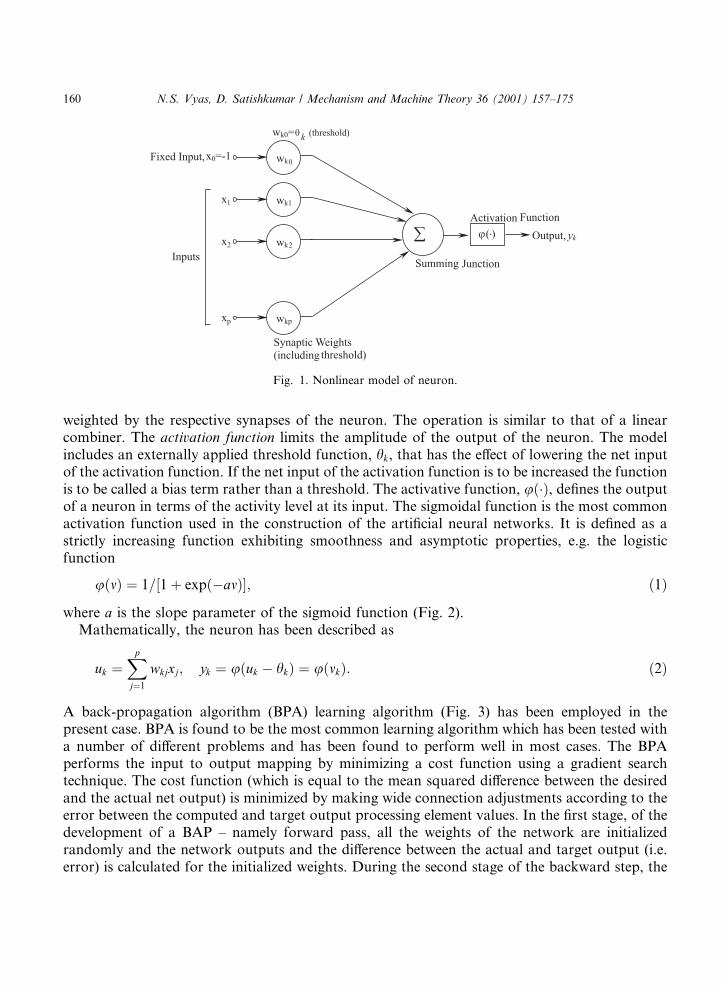
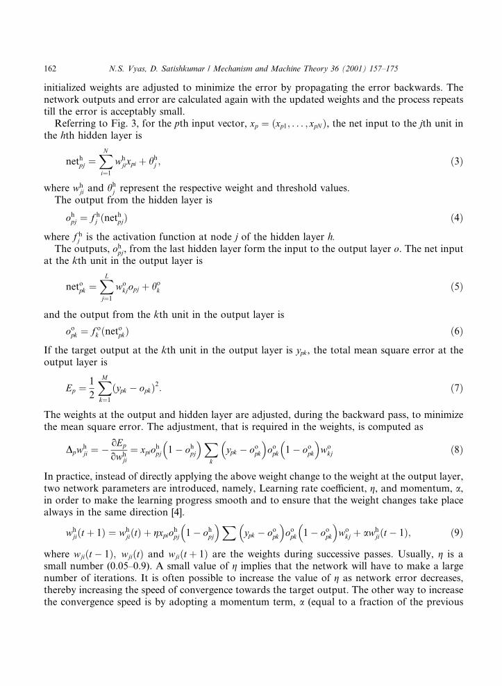
The basic features of the network designed for rotating machinery fault diagnosis are describedhere. Reference, can be made to the text by Hayken [4] for a detailed review of neural networksprocedures. The simulator employs a nonlinear model of a neuron described in Fig. 1. Theconnecting links, called synapses, specify the connection between a signal xj at the input of thesample j,and a neuron k, through a weighting factor, wkj. An adder sums up the input signals
N.S. Vyas, D. Satishkumar / Mechanism and Machine Theory 36 (2001) 157±175 159
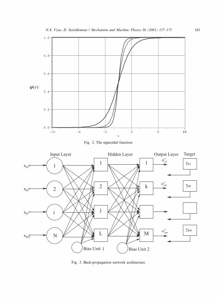
weighted by the respective synapses of the neuron. The operation is similar to that of a linearcombiner. The activation function limits the amplitude of the output of the neuron. The modelincludes an externally applied threshold function, hk, that has the e�ect of lowering the net inputof the activation function. If the net input of the activation function is to be increased the functionis to be called a bias term rather than a threshold. The activative function, u���, de®nes the outputof a neuron in terms of the activity level at its input. The sigmoidal function is the most commonactivation function used in the construction of the arti®cial neural networks. It is de®ned as astrictly increasing function exhibiting smoothness and asymptotic properties, e.g. the logisticfunction
u�m� � 1=�1� exp�ÿam��; �1�where a is the slope parameter of the sigmoid function (Fig. 2).
Mathematically, the neuron has been described as
uk �Xp
j�1
wkjxj; yk � u�uk ÿ hk� � u�mk�: �2�
A back-propagation algorithm (BPA) learning algorithm (Fig. 3) has been employed in thepresent case. BPA is found to be the most common learning algorithm which has been tested witha number of di�erent problems and has been found to perform well in most cases. The BPAperforms the input to output mapping by minimizing a cost function using a gradient searchtechnique. The cost function (which is equal to the mean squared di�erence between the desiredand the actual net output) is minimized by making wide connection adjustments according to theerror between the computed and target output processing element values. In the ®rst stage, of thedevelopment of a BAP ± namely forward pass, all the weights of the network are initializedrandomly and the network outputs and the di�erence between the actual and target output (i.e.error) is calculated for the initialized weights. During the second stage of the backward step, the
Fig. 1. Nonlinear model of neuron.
160 N.S. Vyas, D. Satishkumar / Mechanism and Machine Theory 36 (2001) 157±175
Fig. 3. Back-propagation network architecture.
Fig. 2. The sigmoidal function.
N.S. Vyas, D. Satishkumar / Mechanism and Machine Theory 36 (2001) 157±175 161
initialized weights are adjusted to minimize the error by propagating the error backwards. Thenetwork outputs and error are calculated again with the updated weights and the process repeatstill the error is acceptably small.
Referring to Fig. 3, for the pth input vector, xp � �xp1; . . . ; xpN�, the net input to the jth unit inthe hth hidden layer is
nethpj �
XN
i�1
whjixpi � hh
j ; �3�
where whji and hh
j represent the respective weight and threshold values.The output from the hidden layer is
ohpj � f h
j �nethpj� �4�
where f hj is the activation function at node j of the hidden layer h.
The outputs, ohpj, from the last hidden layer form the input to the output layer o. The net input
at the kth unit in the output layer is
netopk �
XL
j�1
wokjopj � ho
k �5�
and the output from the kth unit in the output layer is
oopk � f o
k �netopk� �6�
If the target output at the kth unit in the output layer is ypk, the total mean square error at theoutput layer is
Ep � 1
2
XM
k�1
�ypk ÿ opk�2: �7�
The weights at the output and hidden layer are adjusted, during the backward pass, to minimizethe mean square error. The adjustment, that is required in the weights, is computed as
Dpwhji � ÿ
oEp
owhji� xpioh
pj 1�ÿ oh
pj
�Xk
ypk
�ÿ oo
pk
�oo
pk 1�ÿ oo
pk
�wo
kj �8�
In practice, instead of directly applying the above weight change to the weight at the output layer,two network parameters are introduced, namely, Learning rate coe�cient, g, and momentum, a,in order to make the learning progress smooth and to ensure that the weight changes take placealways in the same direction [4].
whji t� � 1� � wh
ji�t� � gxpiohpj 1�ÿ oh
pj
�Xypk
�ÿ oo
pk
�oo
pk 1�ÿ oo
pk
�wo
kj � awhji�t ÿ 1�; �9�
where wji�t ÿ 1�; wji�t� and wji�t � 1� are the weights during successive passes. Usually, g is asmall number (0.05±0.9). A small value of g implies that the network will have to make a largenumber of iterations. It is often possible to increase the value of g as network error decreases,thereby increasing the speed of convergence towards the target output. The other way to increasethe convergence speed is by adopting a momentum term, a (equal to a fraction of the previous
162 N.S. Vyas, D. Satishkumar / Mechanism and Machine Theory 36 (2001) 157±175
weight change Dpw), while updating the weights. This additional term tends to keep the weightchanges in the same direction.
3. Network training and testing
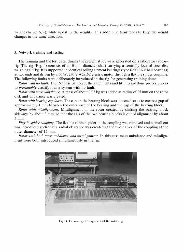
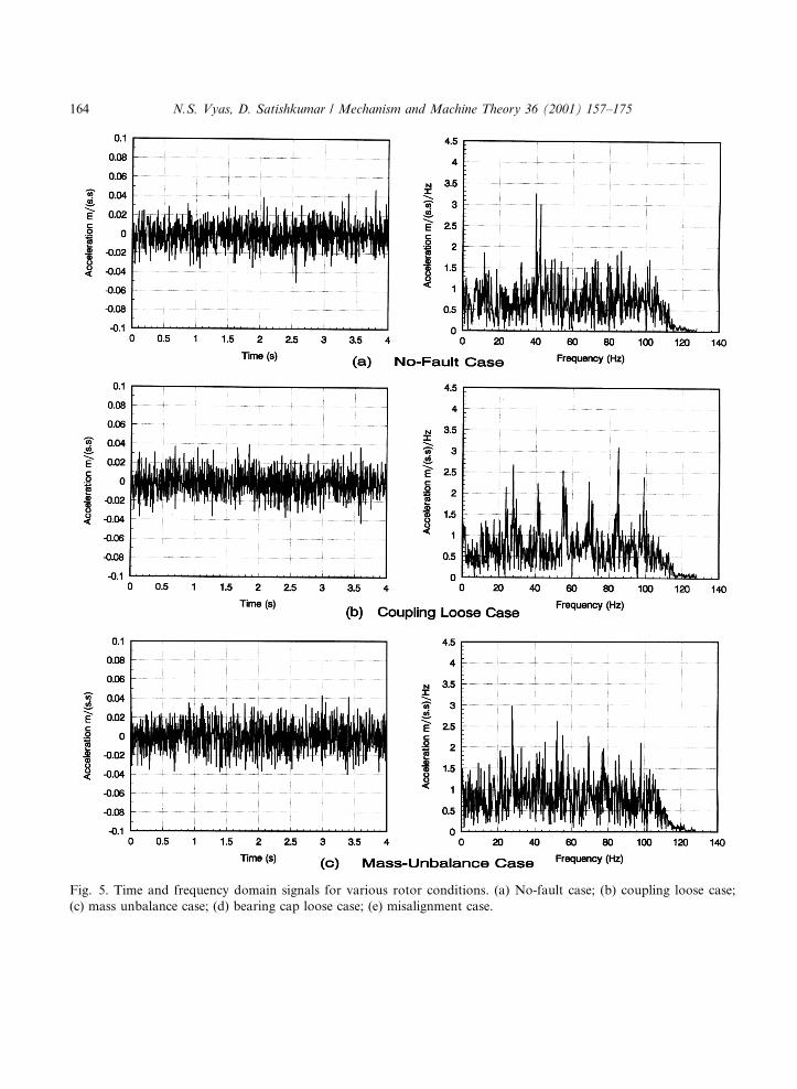
The training and the test data, during the present study were generated on a laboratory rotor±rig. The rig (Fig. 4) consists of a 10 mm diameter shaft carrying a centrally located steel discweighing 0.5 kg. It is supported in identical rolling element bearings (type 6200 SKF ball bearings)at two ends and driven by a 50 W, 230 V AC/DC electric motor through a ¯exible spider coupling.The following faults were deliberately introduced in the rig for generating training data:
Rotor with no fault. The Rotor is balanced, the alignments and ®ttings are done properly so asto presumably classify it as a system with no fault.
Rotor with mass unbalance. A mass of about 0.05 kg was added at radius of 25 mm on the rotordisk and unbalance was created.
Rotor with bearing cap loose. The cap on the bearing block was loosened so as to create a gap ofapproximately 1 mm between the outer race of the bearing and the cap of the bearing block.
Rotor with misalignment. Misalignment in the rotor created by shifting the bearing blocksideways by about 3 mm, so that the axis of the two bearing blocks is out of alignment by about3 mm.
Play in spider coupling. The ¯exible rubber spider in the coupling was removed and a small cutwas introduced such that a radial clearance was created at the two halves of the coupling at theouter diameter of 15 mm.
Rotor with both mass unbalance and misalignment. In this case mass unbalance and misalign-ment were both introduced simultaneously in the rig.
Fig. 4. Laboratory arrangement of the rotor±rig.
N.S. Vyas, D. Satishkumar / Mechanism and Machine Theory 36 (2001) 157±175 163
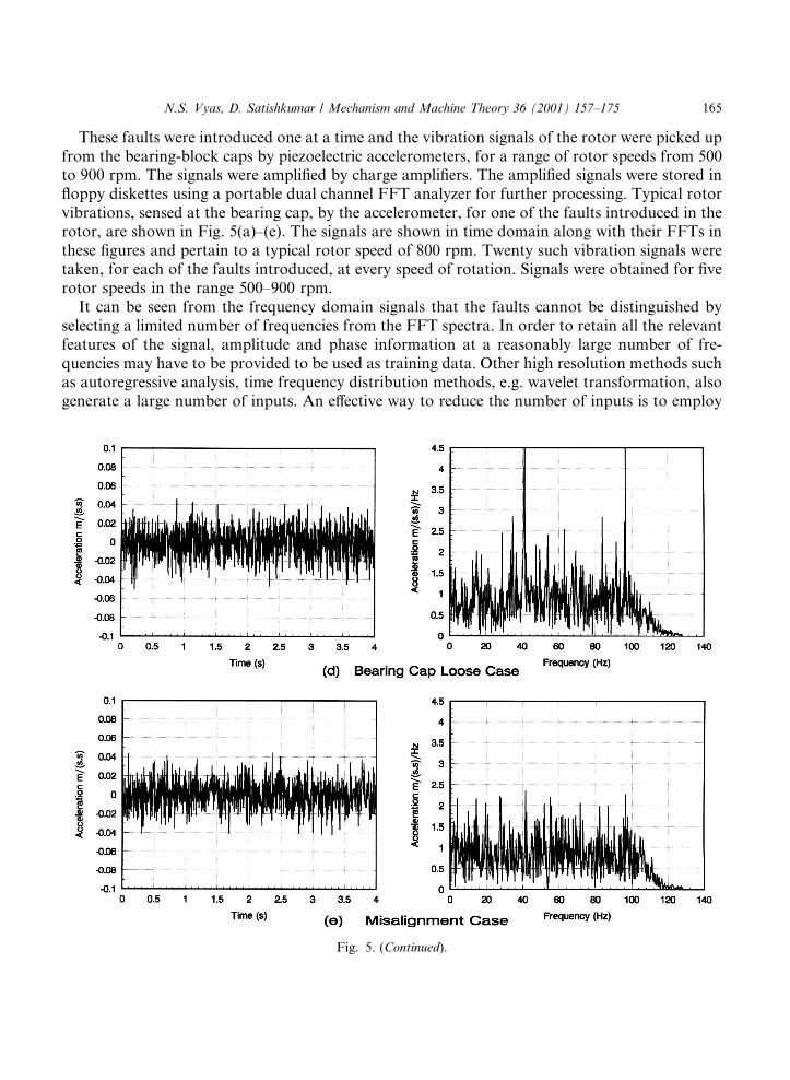
Fig. 5. Time and frequency domain signals for various rotor conditions. (a) No-fault case; (b) coupling loose case;
(c) mass unbalance case; (d) bearing cap loose case; (e) misalignment case.
164 N.S. Vyas, D. Satishkumar / Mechanism and Machine Theory 36 (2001) 157±175
These faults were introduced one at a time and the vibration signals of the rotor were picked upfrom the bearing-block caps by piezoelectric accelerometers, for a range of rotor speeds from 500to 900 rpm. The signals were ampli®ed by charge ampli®ers. The ampli®ed signals were stored in¯oppy diskettes using a portable dual channel FFT analyzer for further processing. Typical rotorvibrations, sensed at the bearing cap, by the accelerometer, for one of the faults introduced in therotor, are shown in Fig. 5(a)±(e). The signals are shown in time domain along with their FFTs inthese ®gures and pertain to a typical rotor speed of 800 rpm. Twenty such vibration signals weretaken, for each of the faults introduced, at every speed of rotation. Signals were obtained for ®verotor speeds in the range 500±900 rpm.
It can be seen from the frequency domain signals that the faults cannot be distinguished byselecting a limited number of frequencies from the FFT spectra. In order to retain all the relevantfeatures of the signal, amplitude and phase information at a reasonably large number of fre-quencies may have to be provided to be used as training data. Other high resolution methods suchas autoregressive analysis, time frequency distribution methods, e.g. wavelet transformation, alsogenerate a large number of inputs. An e�ective way to reduce the number of inputs is to employ
Fig. 5. (Continued).
N.S. Vyas, D. Satishkumar / Mechanism and Machine Theory 36 (2001) 157±175 165
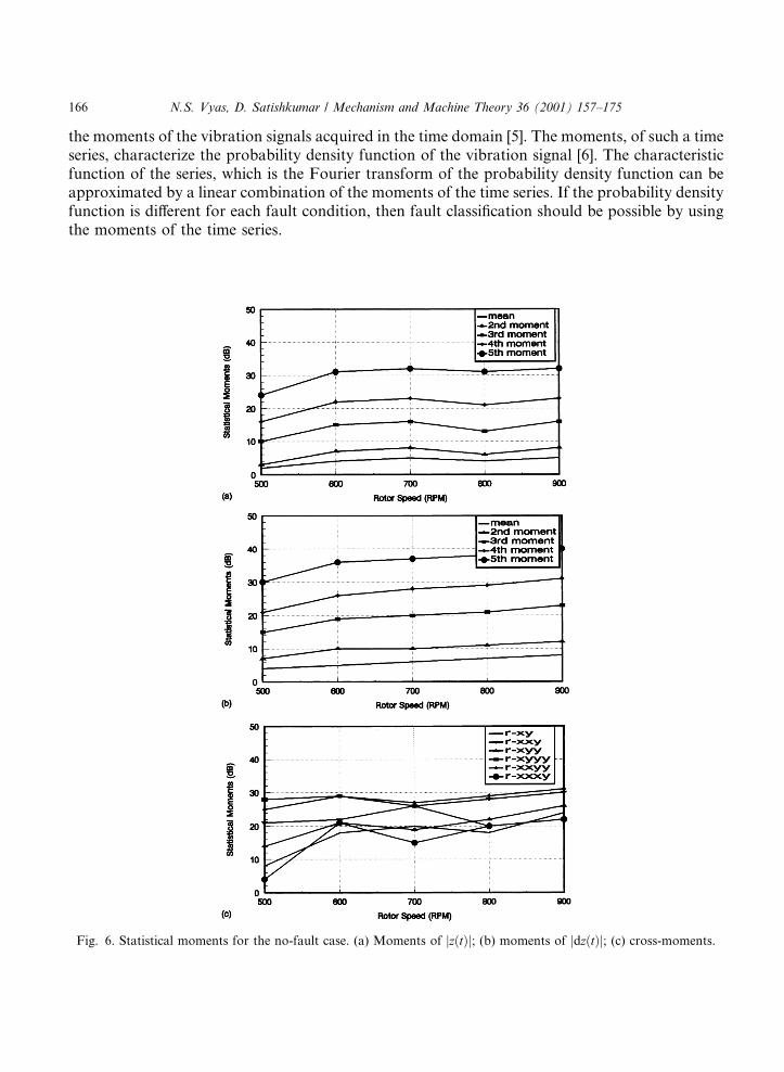
the moments of the vibration signals acquired in the time domain [5]. The moments, of such a timeseries, characterize the probability density function of the vibration signal [6]. The characteristicfunction of the series, which is the Fourier transform of the probability density function can beapproximated by a linear combination of the moments of the time series. If the probability densityfunction is di�erent for each fault condition, then fault classi®cation should be possible by usingthe moments of the time series.
Fig. 6. Statistical moments for the no-fault case. (a) Moments of jz�t�j; (b) moments of jdz�t�j; (c) cross-moments.
166 N.S. Vyas, D. Satishkumar / Mechanism and Machine Theory 36 (2001) 157±175
Representing the data collected by
z�t� � ah�t� � jav�t� and dz�t� � z�t� ÿ z�t ÿ 1�; �10�where ah�t� is the vibration signal from the bearing in the horizontal direction and av�t� is thesignal in the vertical direction, the following moments are computed:· Mean
Efz�t�g � g �Z 1
ÿ1z�t�p�x�dx: �11�
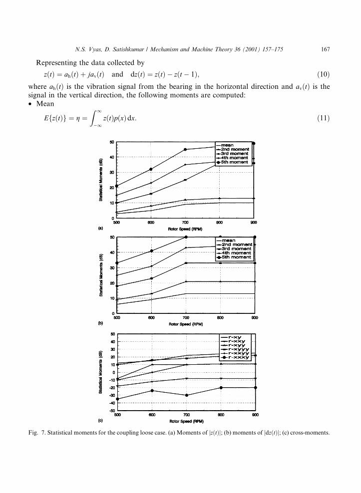
Fig. 7. Statistical moments for the coupling loose case. (a) Moments of jz�t�j; (b) moments of jdz�t�j; (c) cross-moments.
N.S. Vyas, D. Satishkumar / Mechanism and Machine Theory 36 (2001) 157±175 167
· Central moments
lk � Ef�z�t� ÿ g�kg �Z 1
ÿ1�z�t� ÿ g�kp�x�dx; k � 1; 2; 3; . . . �12�
· Cross-moments (cross-correlation)
rxy �X1
t�ÿ1ax�t�ay�t ÿ l�; l � 0;�1;�2: �13�
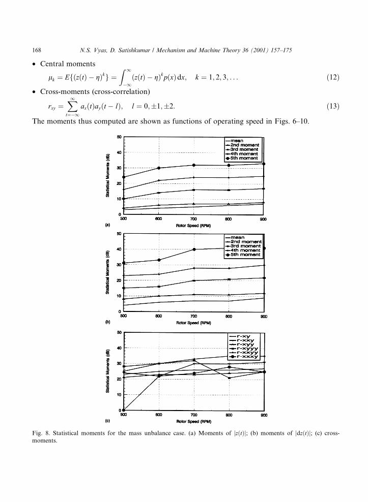
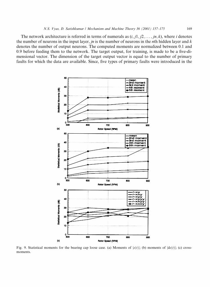
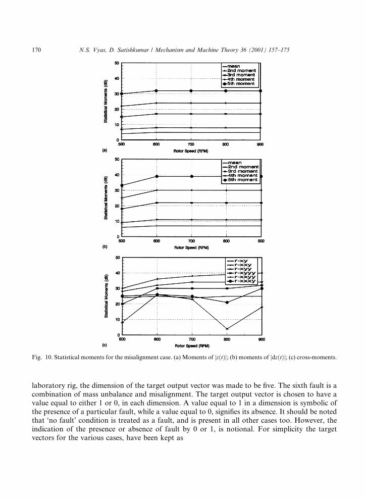
The moments thus computed are shown as functions of operating speed in Figs. 6±10.
Fig. 8. Statistical moments for the mass unbalance case. (a) Moments of jz�t�j; (b) moments of jdz�t�j; (c) cross-
moments.
168 N.S. Vyas, D. Satishkumar / Mechanism and Machine Theory 36 (2001) 157±175
The network architecture is referred in terms of numerals as (i; j1; j2; . . . ; jn; k), where i denotesthe number of neurons in the input layer, jn is the number of neurons in the nth hidden layer and kdenotes the number of output neurons. The computed moments are normalized between 0.1 and0.9 before feeding them to the network. The target output, for training, is made to be a ®ve-di-mensional vector. The dimension of the target output vector is equal to the number of primaryfaults for which the data are available. Since, ®ve types of primary faults were introduced in the
Fig. 9. Statistical moments for the bearing cap loose case. (a) Moments of jz�t�j; (b) moments of jdz�t�j; (c) cross-
moments.
N.S. Vyas, D. Satishkumar / Mechanism and Machine Theory 36 (2001) 157±175 169
laboratory rig, the dimension of the target output vector was made to be ®ve. The sixth fault is acombination of mass unbalance and misalignment. The target output vector is chosen to have avalue equal to either 1 or 0, in each dimension. A value equal to 1 in a dimension is symbolic ofthe presence of a particular fault, while a value equal to 0, signi®es its absence. It should be notedthat `no fault' condition is treated as a fault, and is present in all other cases too. However, theindication of the presence or absence of fault by 0 or 1, is notional. For simplicity the targetvectors for the various cases, have been kept as
Fig. 10. Statistical moments for the misalignment case. (a) Moments of jz�t�j; (b) moments of jdz�t�j; (c) cross-moments.
170 N.S. Vyas, D. Satishkumar / Mechanism and Machine Theory 36 (2001) 157±175
and have been trained accordingly. The vector size could, however, be kept small, for example, bychoosing the set of target vectors as NF 0 0 0; COU 1 0 0 etc.
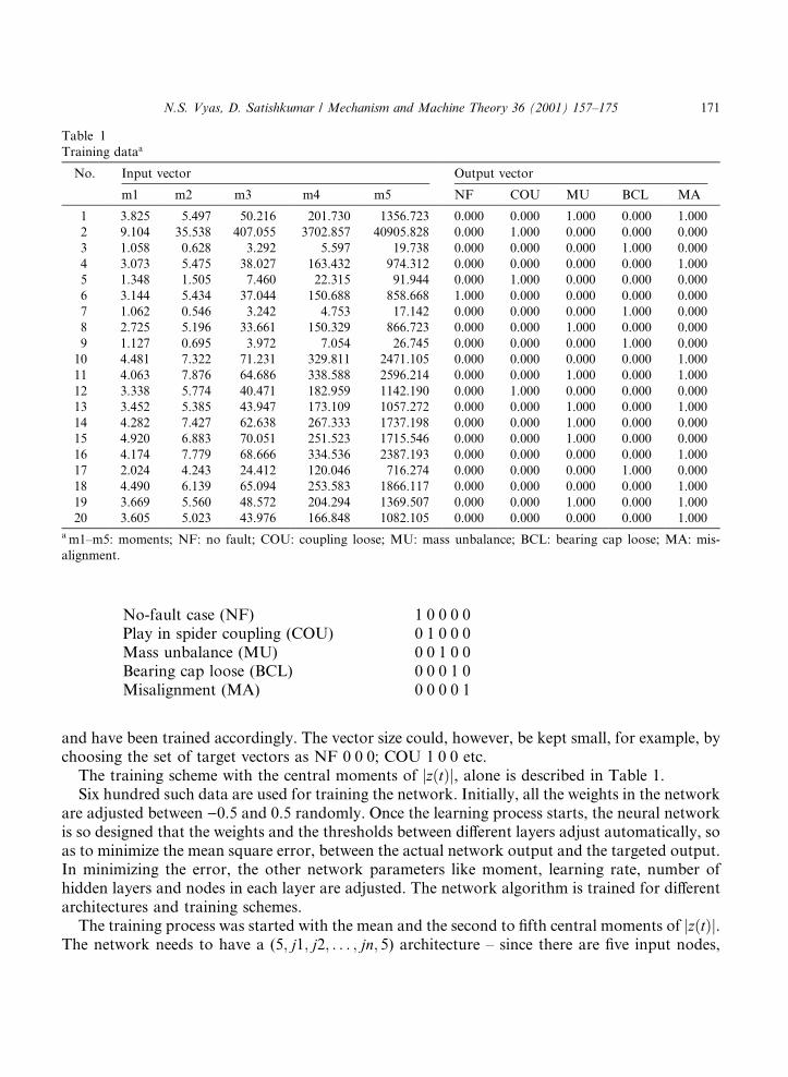
The training scheme with the central moments of jz�t�j, alone is described in Table 1.Six hundred such data are used for training the network. Initially, all the weights in the network
are adjusted between )0.5 and 0.5 randomly. Once the learning process starts, the neural networkis so designed that the weights and the thresholds between di�erent layers adjust automatically, soas to minimize the mean square error, between the actual network output and the targeted output.In minimizing the error, the other network parameters like moment, learning rate, number ofhidden layers and nodes in each layer are adjusted. The network algorithm is trained for di�erentarchitectures and training schemes.
The training process was started with the mean and the second to ®fth central moments of jz�t�j.The network needs to have a (5; j1; j2; . . . ; jn; 5) architecture ± since there are ®ve input nodes,
20 3.605 5.023 43.976 166.848 1082.105 0.000 0.000 0.000 0.000 1.000a m1±m5: moments; NF: no fault; COU: coupling loose; MU: mass unbalance; BCL: bearing cap loose; MA: mis-
alignment.
N.S. Vyas, D. Satishkumar / Mechanism and Machine Theory 36 (2001) 157±175 171
each node corresponding to a moment input; and an output layer consisting of ®ve nodes, eachnode corresponding to one of the ®ve primary faults under consideration. The number of hiddenlayers can be varied. The number of neurons in each hidden layer can also be varied. A total of600 samples, comprising of 100 samples for each fault, was used for the training the network. Anumerical value is required initially, to quantitatively de®ne the accuracy of the training process.A training process will be successful if it is able to correctly identify the fault. The degree of suchaccuracy, called the target error, is the mean square di�erence between a target value (0 or 1) andthe achieved output. To start with, the achievable accuracy was arbitrarily chosen as 0.01. Theoutput vectors which are generated by the network do not always consist of exactly either 0 or 1.
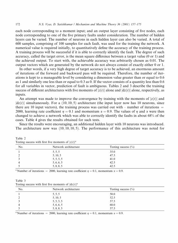
In other words, if a very high degree of target accuracy is to be achieved, an enormous amountof iterations of the forward and backward pass will be required. Therefore, the number of iter-ations is kept to a manageable level by considering a dimension value greater than or equal to 0.6as 1 and similarly one less than or equal to 0.3 as 0. If the vector consists of a quantity less than 0.6for all variables in vector, prediction of fault is ambiguous. Tables 2 and 3 describe the trainingsuccess of di�erent architectures with ®ve moments of jz�t�j alone and jdz�t�j alone, respectively, asinputs.
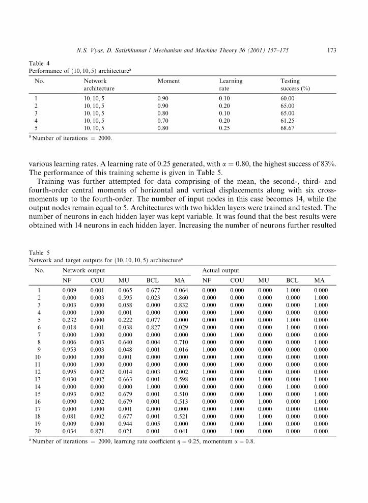
An attempt was made to improve the convergence by training with the moments of jz�t�j andjdz�t�j simultaneously. For a �10; 10; 5� architecture (the input layer now has 10 neurons, sincethere are 10 input vectors), the training process was carried out with ± number of iterations �2000, learning rate coe�cient g � 0:1 and momentum a � 0:9. The values of g and a were thenchanged to achieve a network which was able to correctly identify the faults in about 68% of thecases. Table 4 gives the results obtained for such tests.
Since the results were encouraging, an additional hidden layer with 10 neurons was introduced.The architecture now was �10; 10; 10; 5�. The performance of this architecture was noted for
Table 2
Testing success with ®rst ®ve moments of jz�t�jaNo. Network architecture Testing success (%)
1 5; 5; 5 35.0
2 5; 10; 5 47.5
3 5; 5; 5; 5 41.0
4 5; 6; 6; 5 42.5
5 5; 8; 8; 5 42.5a Number of iterations � 2000, learning rate coe�cient g � 0:1, momentum a � 0:9.
Table 3
Testing success with ®rst ®ve moments of jdz�t�jaNo. Network architecture Testing success (%)
1 5; 5; 5 50.0
2 5; 10; 5 52.5
3 5; 5; 5; 5 57.5
4 5; 6; 6; 5 60.0
5 5; 8; 8; 5 57.5a Number of iterations � 2000, learning rate coe�cient g � 0:1, momentum a � 0:9.
172 N.S. Vyas, D. Satishkumar / Mechanism and Machine Theory 36 (2001) 157±175
various learning rates. A learning rate of 0.25 generated, with a � 0:80, the highest success of 83%.The performance of this training scheme is given in Table 5.
Training was further attempted for data comprising of the mean, the second-, third- andfourth-order central moments of horizontal and vertical displacements along with six cross-moments up to the fourth-order. The number of input nodes in this case becomes 14, while theoutput nodes remain equal to 5. Architectures with two hidden layers were trained and tested. Thenumber of neurons in each hidden layer was kept variable. It was found that the best results wereobtained with 14 neurons in each hidden layer. Increasing the number of neurons further resulted
Table 5
Network and target outputs for �10; 10; 10; 5� architecturea
20 0.034 0.871 0.021 0.001 0.041 0.000 1.000 0.000 0.000 0.000a Number of iterations � 2000, learning rate coe�cient g � 0:25, momentum a � 0:8.
Table 4
Performance of �10; 10; 5� architecturea
No. Network
architecture
Moment Learning
rate
Testing
success (%)
1 10; 10; 5 0.90 0.10 60.00
2 10; 10; 5 0.90 0.20 65.00
3 10; 10; 5 0.80 0.10 65.00
4 10; 10; 5 0.70 0.20 61.25
5 10; 10; 5 0.80 0.25 68.67a Number of iterations � 2000.
N.S. Vyas, D. Satishkumar / Mechanism and Machine Theory 36 (2001) 157±175 173
in overtraining and decreased the success rate. The learning rate and moment were now variedand the network performance was recorded. Table 6 gives this record.
The tests have been carried out for a number of combinations of the learning rate coe�cient gand momentum a, other than those reported in Table 6. The testing success is not found to be anylinear function of these two training parameters and their in¯uence needs to be investigatedfurther. However, for the tests carried out the best results are obtained for the case of learning ratecoe�cient g � 0:1 and momentum a � 0:8, as reported in Table 6. The success rate here is 91%and the network is found to converge to a mean square error of 0.05. A comparison of thenetwork and the actual output for fault identi®cation in this case is shown in Table 7.
Table 6
Testing success for 14 input-architecturea
No. Network architecture Moment Learning rate Testing success (%)
3 14; 14; 14; 5 0.90 0.10 82.85
2 14; 14; 14; 5 0.90 0.15 80.00
5 14; 14; 14; 5 0.90 0.20 87.14
6 14; 14; 14; 5 0.90 0.40 88.57
8 14; 14; 14; 5 0.80 0.10 91.42a Number of iterations � 2000.
Table 7
Network and target outputs for the 14 input-architecturea
20 0.000 1.000 0.000 0.000 0.000 0.000 1.000 0.000 0.000 0.000a Number of iterations � 2000, learning rate coe�cient g � 0:1, momentum a � 0:8.
174 N.S. Vyas, D. Satishkumar / Mechanism and Machine Theory 36 (2001) 157±175
4. Remarks
The study illustrates the e�ectiveness of the arti®cial neural network procedures for fault di-agnosis in a rotor-bearing system. The simulator is found to identify an unknown fault to a gooddegree of accuracy. However, no attempt has been made in this work on quanti®cation of thefault, once it is identi®ed (e.g. estimate of the amount of unbalance, if the fault is identi®ed asunbalance). The focus, presently, was to generate data for healthy and faulty rotor systems anddevelop a preliminary neural network diagnosis frame. It has been found that the testing successin addition to the input and hidden layer architecture, is crucially dependent on the two trainingparameters, namely the learning rate coe�cient and the momentum. These parameters do notshow a linear pattern of behavior and their role needs to be investigated further.