Introduction to Artificial Neural Networkscis.poly.edu/~mleung/CS6673/s09/introductionANN.pdf ·...

POLYTECHNIC UNIVERSITYDepartment of Computer and Information Science

Introduction to Artificial NeuralNetworks

K. Ming Leung

Abstract: A computing paradigm known as artificialneural network is introduced. The differences with theconventional von Neumann machines are discussed.

Directory• Table of Contents• Begin Article

Copyright c© 2008 [email protected] Revision Date: January 22, 2008

mailto:[email protected]

Table of Contents

1. von Neumann Machine and the Symbolic Paradigm

2. The Brain

3. Artificial Neural Networks

4. History

5. Neural Network Computing5.1. Common Activation Functions for Neurons

• Identity Function • Binary Step Function with Threshold• Bipolar Step Function with Threshold • Binary SigmoidFunction • Bipolar Sigmoid Function • An Alternate BipolarSigmoid Function • Nonsaturating Activation Function

5.2. Network Architectures5.3. Network Learning Algorithms

• Supervised Training • Unsupervised Training • Fixed-Weights Nets with no Training

5.4. Applications of NN• NN as logic functions • NN as classifiers

Section 1: von Neumann Machine and the Symbolic Paradigm 3

1. von Neumann Machine and the Symbolic Paradigm

The conventional electronic computer is built according to the vonNeumann machine and the symbolic paradigm.

The basic operations may be modelled by having the computerrepeatedly perform the following cycle of events:

1. The CPU fetches from memory an instruction

2. as well as any data required by the instruction.

3. The CPU then executes the instruction (process the data),

4. and stores the results in memory.

5. Back to step 1.

In this paradigm, it is possible to formalize many problems interms of an algorithm, that is as a well defined procedure or recipewhich, when executed in sequence, will produce the answer. Examplesof such type of problems are the solution to a set of equations or theway to search for an item in a database. The required algorithm maybe broken down into a set of simpler statements which can, in turn,be reduced eventually, to instructions that the CPU executes.

Toc JJ II J I Back J Doc Doc I


In particular, it is possible to process strings of symbols whichrepresent ‘ideas’ or ‘concepts’ and obey the rules of some formal sys-tem. It is the hope in Artificial Intelligence (AI) that all knowledgecould be formalized in such a way: that is, it could be reduced tothe manipulation of symbols according to rules and this manipulationimplemented on a conventional von Neumann machine.

We may draw up a list of the essential characteristics of such ma-chines for comparison with those of neural networks to be discussedlater.

1. The machine must be told in advance, and in great detail, theexact series of steps required to perform the algorithm. Thisseries of steps is specified by the computer program.

2. The type of data it deals with has to be in a precise format -noisy data confuses the machine.

3. The machine can easily fail - destroy a few key memory locationsfor the data or instruction and the machine will stop functioningor ‘crash’.

4. There is a clear correspondence between the semantic objectsToc JJ II J I Back J Doc Doc I


being dealt with (numbers, words, database entries etc) and themachine hardware. Each object can be ‘pointed to’ in a blockof computer memory.

The success of the symbolic approach in AI depends directly onthe consequences of the first point above which assumes we can findan algorithm to describe the solution to the problem. It turns out thatmany everyday tasks we take for granted are difficult to formalize inthis way. For example, our visual (or auditory) recognition of things inthe world; how do we recognize handwritten characters, the particularinstances of which, we may never have seen before, or someone’s facefrom an angle we have never encountered? How do we recall wholevisual scenes on given some obscure verbal cue? The techniques usedin conventional databases are too impoverished to account for thewide diversity of associations we can make.

The way out of these difficulties that will be explored in this courseis to use artificial neural network (ANN) to mimic in some way thephysical architecture of the brain and to emulate brain functions.


Section 2: The Brain 6

2. The Brain

Our brain has a large number (≈ 1011) of highly connected elements(≈ 104 connections per element) called neurons. A neuron has threemajor components: a cell body called soma, one axon, and numerousdendrites. Dendrites are tree-like receptive networks of nerve fibersthat carry electrical signals into the cell body. The cell body has anucleus, and sums and threshold all incoming signals. The axon is along fiber that carries signal from the cell body out to other neurons.

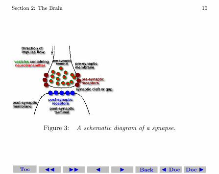
Signals in the brain are transmitted between neurons by electri-cal pulses (action-potentials or ‘spike’ trains) traveling along the axon.The point of contact between an axon of one cell and a dendrite of an-other cell is called a synapse. Each pulse arriving at a synapse initiatesthe release of a small amount of chemical substance or neurotransmit-ter which travels across the synaptic cleft and which is then receivedat post-synaptic receptor sites on the dendritic side of the synapse.The neurotransmitter becomes bound to molecular sites here which,in turn, initiates a change in the dendritic membrane potential. Thispost-synaptic-potential (PSP) change may serve to increase or de-



Figure 1: A schematic diagram of a single neuron.



crease the polarization of the post-synaptic membrane. In the formercase, the PSP tends to inhibit generation of pulses in the afferentneuron, while in the latter, it tends to excite the generation of pulses.The size and type of PSP produced will depend on factors such as thegeometry of the synapse and the type of neurotransmitter. All thesefactors serve to modify the effect of the incoming signal by imposinga certain weight factor. Each PSP will then travel along its dendriteand spread over the cell body of the neuron that is receiving the sig-nal, eventually reaching the base of the axon (axon-hillock). The cellbody sums or integrates the effects of thousands of such PSPs overits dendritic tree and over time. If the integrated potential at theaxon-hillock exceeds a threshold, the cell ‘fires’ and generates an ac-tion potential or spike which starts to travel along its axon. This theninitiates the whole sequence of events again in neurons contained inits pathway.

The way how the neurons are connected together and the natureof the synapses together determine the function of the particular partof the brain. The brain learns new tasks by establishing new pathways and by modifying the strengths of the synapses.



Figure 2: A schematic diagram of a neuron connecting to two otherneurons.



Figure 3: A schematic diagram of a synapse.


Section 3: Artificial Neural Networks 11

Reactions in biological neurons are rather slow (≈ 10−3s) com-pared with electrical circuits inside the CPU (≈ 10−9s), however thebrain can perform certain tasks such as face recognition much fasterthan conventional computers mainly because of the massively paral-lel structure of the biological neural networks (in the sense that allneurons are operating at the same time).

3. Artificial Neural Networks

A Neural Network is an interconnected assembly of simple processingelements, units or nodes, whose functionality is loosely based on theanimal neuron. The processing ability of the network is stored in theinter-unit connection strengths, or weights, obtained by a process ofadaptation to, or learning from, a set of training patterns. In somecases these weights have prescribed values at birth and need not belearned.

Artificial neural networks (ANNs) are not as complex as the brain,but imitate it in the following sense:

1. The building blocks of ANNs are simple computational devices


Section 3: Artificial Neural Networks 12

(capable of summing and thresholding incoming signals).

2. These devices are highly interconnected.

3. Information is processed locally at each neuron.

4. The strength of a synapse is modified by experience (learning).

5. The topological connections between the neurons as well as theconnection strengths determine the function of the ANN.

6. Memory is distributed:• Long-term memory - resides in the synaptic strengths of

neurons.• Short-term memory - corresponds to signal sent by neu-

rons.

7. ANNs are inherently massively parallel.

The advantages of ANN computing are:

1. intrinsically massively parallel.

2. intrinsically fault-tolerant - many brain cells die each day andyet its function does not deteriorate much.


Section 4: History 13

3. capable of learning and generalizing - one can often read someones hand-writing even for the first time.

4. no need to know the underlying laws or governing equations.

Neural networks and conventional algorithmic computers are notin competition but complement each other. There are tasks that aremore suited to an algorithmic approach like arithmetic operations andtasks that are more suited to neural networks. Even more, a largenumber of tasks, require systems that use a combination of the twoapproaches (normally a conventional computer is used to supervisethe neural network) in order to perform at maximum efficiency.

4. History

The history of neural networks that was described above can be di-vided into several periods:

1. First Attempts: There were some initial simulations using for-mal logic. McCulloch and Pitts (1943) developed models of neu-ral networks based on their understanding of neurology. These



models made several assumptions about how neurons worked.Their networks were based on simple neurons which were con-sidered to be binary devices with fixed thresholds. The resultsof their model were simple logic functions such as ”a or b” and”a and b”. Another attempt was by using computer simula-tions. Two groups (Farley and Clark, 1954; Rochester, Holland,Haibit and Duda, 1956). The first group (IBM researchers)maintained closed contact with neuroscientists at McGill Uni-versity. So whenever their models did not work, they consultedthe neuroscientists. This interaction established a multidisci-plinary trend which continues to the present day.

2. Promising and Emerging Technology: Not only was neuroscienceinfluential in the development of neural networks, but psychol-ogists and engineers also contributed to the progress of neuralnetwork simulations. Rosenblatt (1958) stirred considerable in-terest and activity in the field when he designed and developedthe Perceptron. The Perceptron had three layers with the mid-dle layer known as the association layer. This system could



learn to connect or associate a given input to a random outputunit. Another system was the ADALINE (ADAptive LINearElement) which was developed in 1960 by Widrow and Hoff(of Stanford University). The ADALINE was an analogue elec-tronic device made from simple components. The method usedfor learning was different to that of the Perceptron, it employedthe Least-Mean-Squares (LMS) learning rule.

3. Period of Frustration and Low Esteem: In 1969 Minsky and Pa-pert wrote a book in which they generalized the limitations ofsingle layer Perceptrons to multilayered systems. In the bookthey said: ”...our intuitive judgment that the extension (to mul-tilayer systems) is sterile”. The significant result of their bookwas to eliminate funding for research with neural network sim-ulations. The conclusions supported the disenchantment of re-searchers in the field. As a result, considerable prejudice againstthis field was activated.

4. Innovation: Although public interest and available funding wereminimal, several researchers continued working to develop neu-



romorphically based computational methods for problems suchas pattern recognition. During this period several paradigmswere generated which modern work continues to enhance. Gross-berg’s (Steve Grossberg and Gail Carpenter in 1988) influencefounded a school of thought which explores resonating algo-rithms. They developed the ART (Adaptive Resonance The-ory) networks based on biologically plausible models. Andersonand Kohonen developed associative techniques independent ofeach other. Klopf (A. Henry Klopf) in 1972, developed a ba-sis for learning in artificial neurons based on a biological prin-ciple for neuronal learning called heterostasis. Werbos (PaulWerbos 1974) developed and used the back-propagation learn-ing method, however several years passed before this approachwas popularized. Back-propagation nets are probably the mostwell known and widely applied of the neural networks today. Inessence, the back-propagation net is a Perceptron with multiplelayers, a different threshold function in the artificial neuron, anda more robust and capable learning rule. Amari (A. Shun-Ichi1967) was involved with theoretical developments: he published



a paper which established a mathematical theory for a learningbasis (error-correction method) dealing with adaptive patternclassification. While Fukushima (F. Kunihiko) developed a stepwise trained multilayered neural network for interpretation ofhandwritten characters. The original network was published in1975 and was called the Cognitron.

5. Re-Emergence: Progress during the late 1970s and early 1980swas important to the re-emergence on interest in the neural net-work field. Several factors influenced this movement. For exam-ple, comprehensive books and conferences provided a forum forpeople in diverse fields with specialized technical languages, andthe response to conferences and publications was quite positive.The news media picked up on the increased activity and tu-torials helped disseminate the technology. Academic programsappeared and courses were introduced at most major Universi-ties (in US and Europe). Attention is now focused on fundinglevels throughout Europe, Japan and the US and as this fund-ing becomes available, several new commercial applications in


Section 5: Neural Network Computing 18

industry and financial institutions are emerging.

6. Today: Significant progress has been made in the field of neuralnetworks enough to attract a great deal of attention and fundfurther research. Advancement beyond current commercial ap-plications appears to be possible, and research is advancing thefield on many fronts. Neurally based chips are emerging andapplications to complex problems developing. Clearly, today isa period of transition for neural network technology.

5. Neural Network Computing

An artificial neural network (ANN) consists of a large number ofhighly connected artificial neurons. We will consider the differentchoices of neurons used in an ANN, the different types of connectivity(architecture) among the neurons, and the different schemes for mod-ifying the weight factors connecting the neurons. From here on, it isclear that we are not actually dealing with the real biological neuronnetwork, we will often drop the word ”artificial” and simply refer towhat we do as neural network (NN).



5.1. Common Activation Functions for Neurons

Let us denote the weighted sum of input into a neuron by yin. Theactivation or output of the neuron, y, is then given by applying theactivation (or transfer) function, f , to yin:

y = f(yin).

The activation function should be a rather simple function. Sometypical choices are given below.

• Identity FunctionIf f is an identity function,

y = f(yin) = yin,

the activation (output) of the neuron is exactly the same as theweighted sum of the input into the neuron. As we will see later,identity activation functions are used for neurons in the input layerof an ANN.



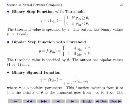
• Binary Step Function with Threshold

y = f(yin) =

{1 if yin ≥ θ,0 if yin < θ.

The threshold value is specified by θ. The output has binary values(0 or 1) only.

• Bipolar Step Function with Threshold

y = f(yin) =

{1 if yin ≥ θ,−1 if yin < θ.

The threshold value is specified by θ. The output has bipolar values(1 or -1) only.

• Binary Sigmoid Function

y = f(yin) =1

1 + e−σ(yin−θ)

,

where σ is a positive parameter. This function switches from 0 to1 in the vicinity of θ as the argument goes from −∞ to +∞. The



larger the values of σ is the more abrupt the change occurs. Unlikethe above step functions, the binary Sigmoid function is smooth. Infact it has a derivative which is also smooth. It is easy to see that itsderivative is given by

f ′(yin) = σf(yin)[1− f(yin)].

Thus its derivative can be easily computed from the value of the orig-inal function itself.

• Bipolar Sigmoid Function

y = f(yin) = tanh(σ

2(yin − θ)

),

where σ is a positive parameter. This function switches from -1 to 1in the vicinity of θ as the argument goes from −∞ to +∞. The largerthe values of σ is the more abrupt the change occurs. The bipolarSigmoid function is also smooth with a smooth derivative given by

f ′(yin) =σ

2[1 + f(yin)

] [1− f(yin)

].



−1 0 1 2 3

0

0.5

1binary step

−1 0 1 2 3

−1

0

1

bipolar step

−5 0 50

0.5

1

binary sigmoid

−5 0 5−1

0

1

bipolar sigmoid

−5 0 5

−1

0

1

arctangent

−10 −5 0 5 10

−2

0

2

non−saturating

Figure 4: Some common transfer functions.



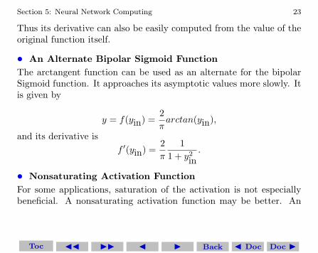
Thus its derivative can also be easily computed from the value of theoriginal function itself.

• An Alternate Bipolar Sigmoid FunctionThe arctangent function can be used as an alternate for the bipolarSigmoid function. It approaches its asymptotic values more slowly. Itis given by

y = f(yin) =2π

arctan(yin),

and its derivative isf ′(yin) =

2π

11 + y2

in.

• Nonsaturating Activation FunctionFor some applications, saturation of the activation is not especiallybeneficial. A nonsaturating activation function may be better. An



example of such function is

y = f(yin) =

{log(1 + yin) if yin ≥ 0,

− log(1 + yin) if yin < 0.

Note that the derivative is continuous at the origin:

f ′(yin) =

1

1+yinif yin ≥ 0,

11−yin

if yin < 0.

5.2. Network Architectures

The way how the neurons are connected to each other plays an im-portant role in determining the function of a neural network.

It is often convenient to visualize neurons as arranged in layers.Neurons in the same layer have the same basic characteristics, that isthey have the same form of activation function, and the same patternof connections to the other neurons. However, they are expected tohave different connection strengths and threshold values.

A NN typically have an input layer where the neurons all have



activation functions given by the identity function. A signal entersthe ANN from the input layer. It also has an output layer, where theoutput for each neuron is given by y.

All the remaining neurons in the NN are organized into layersknown as the hidden layers. Neurons within a layer are connected tothe neurons in its adjacent layer. There may be 0, 1, or more suchhidden layers. NNs are classified by the total number of layers, notcounting the input layer.

An ANN is called a feedforward net if the input signal going intothe input layer propagates through each of the hidden layers andfinally emerge from the output layer.

The figure shows the simplest of such a feedforward NN. There areN neurons in the input layer and they are labeled by X1, X2, . . . , XN .The signal in those neurons are denoted by x1, x2, . . . , xN , respec-tively. There is just a single output neuron, labeled by Y . The signalthere, denoted by y, is the output signal of the network. The strengthsof the connections between the input neurons and the output neuronare labeled by w1, w2, . . . , wN , respectively.

The input signal, represented by a vector (x1, x2, . . . , xN ), is trans-Toc JJ II J I Back J Doc Doc I


X1

X2

Xn

Y

x1

x2

xn

y

w1

w2

wn

Figure 5: The simplest feedforward NN having 1 output neuron.



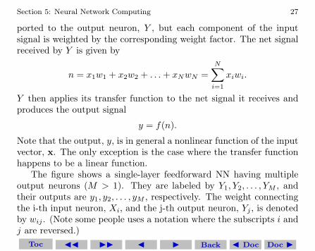
ported to the output neuron, Y , but each component of the inputsignal is weighted by the corresponding weight factor. The net signalreceived by Y is given by

n = x1w1 + x2w2 + . . . + xNwN =N∑

i=1

xiwi.

Y then applies its transfer function to the net signal it receives andproduces the output signal

y = f(n).

Note that the output, y, is in general a nonlinear function of the inputvector, x. The only exception is the case where the transfer functionhappens to be a linear function.

The figure shows a single-layer feedforward NN having multipleoutput neurons (M > 1). They are labeled by Y1, Y2, . . . , YM , andtheir outputs are y1, y2, . . . , yM , respectively. The weight connectingthe i-th input neuron, Xi, and the j-th output neuron, Yj , is denotedby wij . (Note some people uses a notation where the subscripts i andj are reversed.)



X1

X2

Xn

Y1

Y2

Ym

x1

x2

xn

y1

y2

ym

w11

w12

w13

w21

w22

w23

w31w32

w33

Figure 6: A single-layer feedforward NN having multiple output neu-rons.



A layer is called recurrent if it has closed-loop connection from aneuron back to itself.

5.3. Network Learning Algorithms

Algorithms for setting the weights of the connections between neuronsare also called learning or training rules. There are three basic typesof training rule.

• Supervised TrainingIn supervised training, the network is trained by presenting it a se-quence of training inputs (patterns), each with an associated targetoutput value. Weights in the net are adjusted according to a learningalgorithm.

• Unsupervised TrainingIn unsupervised training, a sequence of training inputs is provided,but no target output values are specified. The weights are adjustedaccording to a learning algorithm.



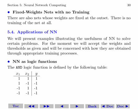
• Fixed-Weights Nets with no TrainingThere are also nets whose weights are fixed at the outset. There is notraining of the net at all.

5.4. Applications of NN

We will present examples illustrating the usefulness of NN to solvecertain problems. For the moment we will accept the weights andthresholds as given and will be concerned with how they are obtainedthrough appropriate training processes.

• NN as logic functionsThe AND logic function is defined by the following table:

x1 x2 y1 1 11 -1 -1

-1 1 -1-1 -1 -1



X1

X2

Y

x1

x2

y

w1

w2

Figure 7: A single-layer feedforward NN having 2 input and 1 outputneurons.

We are using bipolar values here rather than binary ones, andso the transfer function used for the output neuron is the bipolarstep function. A NN with two input neurons and a single outputneuron can operate as an AND logic function if we choose weightsw1 = 1, w2 = 1 and threshold θ = 1. We can verify that for

x1 = 1, x2 = 1 : n = 1× 1 + 1× 1 = 2 is > 1 so y = 1

x1 = 1, x2 = −1 : n = 1× 1 + 1× (−1) = 0 is < 1 so y = −1x1 = −1, x2 = 1 : n = 1× (−1) + 1× 1 = 0 is < 1 so y = −1

x1 = −1, x2 = −1 : n = 1×(−1)+1×(−1) = −2 is < 1 so y = −1Toc JJ II J I Back J Doc Doc I


Note that many other choices for the weights and threshold will alsowork.

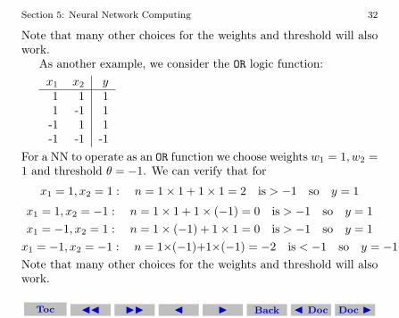
As another example, we consider the OR logic function:x1 x2 y1 1 11 -1 1

-1 1 1-1 -1 -1

For a NN to operate as an OR function we choose weights w1 = 1, w2 =1 and threshold θ = −1. We can verify that for

x1 = 1, x2 = 1 : n = 1× 1 + 1× 1 = 2 is > −1 so y = 1

x1 = 1, x2 = −1 : n = 1× 1 + 1× (−1) = 0 is > −1 so y = 1x1 = −1, x2 = 1 : n = 1× (−1) + 1× 1 = 0 is > −1 so y = 1

x1 = −1, x2 = −1 : n = 1×(−1)+1×(−1) = −2 is < −1 so y = −1Note that many other choices for the weights and threshold will alsowork.



As we will see in the next chapter, the NN as defined above cannotperform the XOR logic function:

x1 x2 y1 1 -11 -1 1

-1 1 1-1 -1 -1

no matter what the values of the weights and threshold are. NNhaving a different architecture is needed.

• NN as classifiersOther than operating as a logic function, NN can also be used tohandle classification problems. For example, we want to classify cus-tomers into two classes. Class 1 are those who will likely buy a ridinglawn-mower, and class 2 are those who will likely not do so. Thedecision is based on the customer’s income and lawn size. For eachcustomer, there is a vector

x = (x1, x2),



where x1 is the income in units of 100, 000 dollars, and x2 is the lawnsize in acres. For this example, we use the same NN with weightsw1 = 0.7, w2 = 1.1 and threshold θ = 2.3.

Using this NN, we find that a customer who makes 30, 000 a yearand has a lawn size of 2 acres will likely buy a riding lawn-mower,since the net signal received by Y

0.3× 0.7 + 2× 1.1 = 0.21 + 2.2 = 2.41

is larger than the threshold theta = 2.3. On the other hand, a cus-tomer who makes 150, 000 a year and has a lawn size of 1 acre willlikely not buy a riding lawn-mower, since the net signal received byY

1.5× 0.7 + 1× 1.1 = 1.05 + 1.1 = 2.15is smaller than the threshold.

In real applications, input vectors typically have a large numberof components (i.e. N � 1).



References

[1] Laurene Fausett, ”Fundamentals of Neural Networks - Architec-tures, Algorithms, and Applications”, Prentice Hall, 1994.


Date post:	01-Apr-2018
Category:	Documents
Upload:	vunga
View:	227 times
Download:	2 times

Introduction to Artificial Neural Networkscis.poly.edu/~mleung/CS6673/s09/introductionANN.pdf ·...

Documents