Artificial Neural Networks vs.

Support Vector Machines for

Skin Diseases Recognition

Micha l Antkowiak

May 3, 2006

Master’s Thesis in Computing Science, 20 creditsSupervisor at CS-UmU: Michael Minock

Examiner: Per Lindstrom

Umea University

Department of Computing Science

SE-901 87 UMEA

SWEDEN

Abstract

Artificial Neural Networks (ANNs) as well as Support Vector Machines (SVM) are verypowerful tools which can be utilized for pattern recognition. They are being used ina large array of different areas including medicine. This thesis exemplifies the applica-bility of computer science in medicine, particularly dermatological tools and softwarewhich uses ANN or SVM. Basic information about ANN, including description of Back-Propagation Learning Algorithm, has also been introduced as well as information aboutSVM.

Finally the system for recognition of skin diseases, called Skinchecker, is described.Skinchecker has been developed in two versions: using ANN and SVM. Both versionshave been tested and their results of recognition of skin diseases from pictures of theskin fragments are compared and presented here.

ii

Contents

1 Introduction 1

2 Background 3

2.1 Computer science in medicine . . . . . . . . . . . . . . . . . . . . . . . . 3

2.1.1 Dermatological tools . . . . . . . . . . . . . . . . . . . . . . . . . 3

2.1.2 ANN use in medicine . . . . . . . . . . . . . . . . . . . . . . . . . 4

2.1.3 SVM use in medicine . . . . . . . . . . . . . . . . . . . . . . . . . 4

2.2 Neural networks . . . . . . . . . . . . . . . . . . . . . . . . . . . . . . . 5

2.2.1 Biological neural networks . . . . . . . . . . . . . . . . . . . . . . 5

2.2.2 Introduction to ANNs . . . . . . . . . . . . . . . . . . . . . . . . 6

2.2.3 Training of the ANN . . . . . . . . . . . . . . . . . . . . . . . . . 9

2.3 Support Vector Machines . . . . . . . . . . . . . . . . . . . . . . . . . . 11

2.3.1 Kernel functions . . . . . . . . . . . . . . . . . . . . . . . . . . . 11

2.3.2 Multi-class classification . . . . . . . . . . . . . . . . . . . . . . . 12

3 Approach 15

3.1 Recognition of skin diseases . . . . . . . . . . . . . . . . . . . . . . . . . 15

3.2 Chosen diseases . . . . . . . . . . . . . . . . . . . . . . . . . . . . . . . . 15

3.3 Dataset . . . . . . . . . . . . . . . . . . . . . . . . . . . . . . . . . . . . 18

3.3.1 Image preprocessing . . . . . . . . . . . . . . . . . . . . . . . . . 19

3.4 Skinchecker with ANN . . . . . . . . . . . . . . . . . . . . . . . . . . . . 19

3.5 Skinchecker with SVM . . . . . . . . . . . . . . . . . . . . . . . . . . . . 19

4 Results 21

4.1 Results for ANN . . . . . . . . . . . . . . . . . . . . . . . . . . . . . . . 21

4.1.1 Quickprop algorithm . . . . . . . . . . . . . . . . . . . . . . . . . 21

4.1.2 Incremental algorithm . . . . . . . . . . . . . . . . . . . . . . . . 22

4.2 Results for SVM . . . . . . . . . . . . . . . . . . . . . . . . . . . . . . . 23

4.3 Comparison . . . . . . . . . . . . . . . . . . . . . . . . . . . . . . . . . . 24

4.4 Cross validation testing . . . . . . . . . . . . . . . . . . . . . . . . . . . 25

iii

iv CONTENTS

5 Conclusions 27

5.1 Limitations . . . . . . . . . . . . . . . . . . . . . . . . . . . . . . . . . . 27

5.2 Future work . . . . . . . . . . . . . . . . . . . . . . . . . . . . . . . . . . 27

6 Acknowledgements 29

References 31

A Back-Propagation Learning Algorithm description 35

A.1 Training . . . . . . . . . . . . . . . . . . . . . . . . . . . . . . . . . . . . 35

A.2 Classification . . . . . . . . . . . . . . . . . . . . . . . . . . . . . . . . . 36

List of Figures

2.1 Two connected biological neurons . . . . . . . . . . . . . . . . . . . . . . 5

2.2 Model of an artificial neuron . . . . . . . . . . . . . . . . . . . . . . . . 6

2.3 Multilayer feed-forward ANN . . . . . . . . . . . . . . . . . . . . . . . . 7

2.4 Selection of the number of layers for solving different problems . . . . . 8

2.5 Multilayer feedback ANN . . . . . . . . . . . . . . . . . . . . . . . . . . 8

2.6 Back-propagation of errors values . . . . . . . . . . . . . . . . . . . . . . 10

2.7 Optimal hyperplane . . . . . . . . . . . . . . . . . . . . . . . . . . . . . 11

2.8 Transformation of input space into feature space . . . . . . . . . . . . . 12

3.1 Exemplary pictures of diseases . . . . . . . . . . . . . . . . . . . . . . . 17

3.2 Skinchecker-DataSet module . . . . . . . . . . . . . . . . . . . . . . . . . 18

4.1 Training the ANN using quickprop algorithm . . . . . . . . . . . . . . . 22

4.2 Training the ANN using incremental algorithm . . . . . . . . . . . . . . 23

4.3 Comparison of results . . . . . . . . . . . . . . . . . . . . . . . . . . . . 24

v

vi LIST OF FIGURES

List of Tables

3.1 Diseases chosen for training the system. . . . . . . . . . . . . . . . . . . 16

4.1 Results for quickprop algorithm . . . . . . . . . . . . . . . . . . . . . . . 21

4.2 Number of epochs for incremental training. . . . . . . . . . . . . . . . . 22

4.3 Results for incremental algorithm . . . . . . . . . . . . . . . . . . . . . . 23

4.4 Results for SVM . . . . . . . . . . . . . . . . . . . . . . . . . . . . . . . 24

4.5 Cross validation testing . . . . . . . . . . . . . . . . . . . . . . . . . . . 25

vii

viii LIST OF TABLES

Chapter 1

Introduction

Skin diseases are now very common all over the world. For example the number ofpeople with skin cancer has doubled in the past 15 years. “Currently, between 2 and 3million non-melanoma skin cancers and 132,000 melanoma skin cancers occur globallyeach year. One in every three cancers diagnosed is a skin cancer and, according to SkinCancer Foundation Statistics, one in every five Americans will develop skin cancer intheir lifetime” [42]. Different kinds of allergies are also becoming more common. Manyof these diseases are very dangerous, particularly when not treated at an early stage.Dermatologists have at their disposal large catalogues with pictures of skin segments,which they use as a reference for diagnosis of their patients cases’ skin ailments [10].However it may be difficult even for experienced doctors, to make correct diagnosisbecause many symptoms look very similar to each other, even though they are causedby different diseases. All details such as colour, size or density of the skin changes areimportant. Modern medicine is looking for solutions, which could help doctors with anyaspect of their work using the new technology. Such tools already exist, to our knowledgethey concentrate on analysis of the colour of skin changes and UV photography [7, 38].

Although these tools are commercially available, there seems to be a lot of room forfurther improvement. The goal of this project is to make a system to recognize skindiseases using Artificial Neural Networks (ANNs) and Support Vector Machines (SVM).After testing both methods results will be compared. System should learn from theset of skin segments images taken by digital camera. After that it should return theprobability of existence of any recognized disease, based on the same type of image madeby user. Images should have the same size and should be taken from the same distance.Some practical study may display need of using other information (not only pictures) totrain the network, for example part of the body where the symptoms were found or ifthe patient feels pain or tickle. Program can also provide some tools that will be foundas useful during the study.

Artificial Neural Networks are one of the most efficient methods for pattern recog-nition [3, 4, 30, 35, 37]. They are used as a model for simulation of the workings ofa brain. They cannot replace a doctor, but ANNs can help him in diagnosis [2]. AlsoSVM is used for pattern recognition and is achieving good accuracy. It expands veryquickly and is more and more popular [34, 36]. It can be very useful in many types ofapplications, also in dermatology.

1

2 Chapter 1. Introduction

Chapter 2

Background

2.1 Computer science in medicine

Computer science has been widely adopted by modern medicine. One reason is that anenormous amount of data has to be gathered and analysed which is very hard or evenimpossible without making use of computer systems. The majority of medical tools areable to send results of their work directly to a computer facilitating significantly collec-tion of necessary information. Computer systems can also lower the risk of misdiagnosis.In the experiment described in [27] an ANN-trained computer, an experienced dermatol-ogist and an inexperienced clinician with minimal training were diagnosing melanoma.Results of the first two diagnoses were similar and were also better than the resultsof the inexperienced clinician. It shows that computer-aided diagnosis can be a veryhelpful tool, particularly in areas which lack experienced specialists.

A large number of such tools already exists and they provide an aid to the doctorsin their everyday work [7]. In this paper we are concerned with dermatology, ANNs andSVM, therefore some tools applied in this area will be described.

2.1.1 Dermatological tools

Dermatology can be described as a branch of medicine primarily concerned with skinand its diseases. It is one of the most difficult areas in medicine. It demands detailedknowledge and experience [19]. Fortunately dermatologists are now aided by a numberof modern inventions which makes their work easier and produces better results forpatients.

A very important task of a doctor is to make the correct diagnosis of the illness aswell as to estimate its progress. To remember and register the actual state of patients,doctors use some scoring systems. However, there are some factors which cause lack ofobjectivity in these systems. A problem can ensue when a patient changes his doctor.Previously given scores can be misunderstood because they may vary from doctor todoctor. Some discrepancy can also appear between scores taken by the same doctor indifferent circumstances. To avoid the human partiality in psoriasis scoring a computersystem is proposed in [14].

Digital image analysis role in dermatology has increased recently. Many algorithmsfrom this area are used to diagnose different diseases. A highly efficient algorithm fordiagnosis of melanocytic lesions is described in [5]. After the experiment it turned out

3

4 Chapter 2. Background

that the algorithm developed by [5] can achieve similar accuracy as the dermoscopicclassification rules applied by dermatologists. However, a dermatologist is still requiredto recognize if lesions are of a melanocytic nature.

Some dermatological problems are considered to be very difficult, for example the dif-ferential diagnosis of erythemato-squamous diseases. Differences between various typesof this illness can be very small; therefore the probability of wrong diagnosis can be signif-icant. To lower it, an expert system which consists of the three classification algorithmsis proposed in [15]. A program, called DES1, uses the nearest neighbour classifier, naiveBayesian classifier and voting feature intervals-5. A combination of these algorithmsachieves better results and helps to avoid mistakes in diagnosis. According to [15] DEScan be used not only by dermatologists but also by students for testing their knowledge.Another useful feature is a database of the patient records.

2.1.2 ANN use in medicine

ANNs’ effectiveness in recognizing patterns and relations is a reason why they are beingused to aid doctors in solving medical problems. Until 1996 they have not been used inthis area frequently; they have been generally applied in radiology, urology, laboratorymedicine and cardiology [20]. Recently ANNs have proven to be useful in many otherfields of medicine including dermatology. They have shown large efficiency not only indiagnosis but also in modelling parts of the human body.

One of the most important dermatological problems is melanoma diagnosis. Der-matologists achieve accuracy in recognizing malignant melanoma between 65 and 85%,whereas early detection means decreasing of mortality. System using genetic algorithmsand ANNs, proposed in [16], reached 97.7% precision. In the system proposed in [13]85% sensitivity and 99% specificity were achieved for diagnosis of melanoma.

Another developed system for computer-aided diagnosis of pigmented skin lesions isdemonstrated in [17]. Diagnostic and neural analysis of skin cancer (DANAOS) showedthe results comparable to results of dermatologists. It was also found that imageshard to recognize by DANAOS differed from those causing problems to dermatologists.Cooperation between humans and computers could therefore lower the probability ofmistakes. Results obtained are also dependent on the size and quality of the databaseused.

ANNs have also been adopted in pharmaceutical research [1] and in many otherdifferent clinical applications using pattern recognition; for example: diagnosis of breastcancer, interpreting electrocardiograms, diagnosing dementia, predicting prognosis andsurvival rates [38].

2.1.3 SVM use in medicine

SVM is not so well known as the ANN. However, it was also applied to some medicaltools. One of them, proposed in [33], identifies patients with breast cancer for whomchemotherapy could prolong survival time. In the experiment SVM was used for classi-fying patients into one of three possible prognostic groups: Good, Poor or Intermediate.After classification of 253 patients, 82.7% test set correctness was achieved.

Another application of SVM in medicine is described in [18]. A system for cancerdiagnosis used the DNA micro-array data as a classification data set. Diagnosis error

1Diagnosis of Erythemato-Squamous

2.2. Neural networks 5

obtained by above mentioned system was smaller than in systems which uses otherknown methods. Reduction of the error achieved 36%.

SVM is relatively new method of classification and it expands very quickly. Thatwill certainly cause wider use of SVM in different areas, also in medicine.

2.2 Neural networks

The ANNs consist of many connected neurons simulating a brain at work. A basicfeature which distinguishes an ANN from an algorithmic program is the ability to gen-eralize the knowledge of new data which was not presented during the learning process.Expert systems need to gather actual knowledge of its designated area. However, ANNsonly need one training and show tolerance for discontinuity, accidental disturbances oreven defects in the training data set. This allows for usage of ANNs in solving problemswhich cannot be solved by other means effectively [3, 35]. These features and advantagesare the reason why the area of ANN’s application is very wide and includes for example:

– Pattern recognition,

– Object classification,

– Medical diagnosis,

– Forecast of economical risk, market prices changes, need for electrical power, etc.,

– Selection of employees,

– Approximation of function value.

2.2.1 Biological neural networks

The human brain consists of around 1011 nerve cells called neurons (see Fig. 2.1). The

axon

dendrites

synapse

Figure 2.1: Two connected biological neurons. The black area inside a cell body iscalled nucleus. A signal is send along the axon and through the synapse is transferredto dendrites of the other neuron (taken from [3] with permission).

nucleus can be treated as the computational centre of a neuron. Here the main processestake place. The output duct of a neuron is called axon whereas dendrite is its input. Oneneuron can have many dendrites but only one axon; biological neurons have thousands ofdendrites. Connections between neurons are called synapses; their quantity in a human

6 Chapter 2. Background

brain is greater than 1014. A neuron receives electrical impulses through its dendritesand sends them to the next neurons using axon. An axon is split into many branchesending with synapses. Synapses change power of received signal before the next neuronwill receive it. Changing the strengths of synapse effects is assumed to be a crucial partof learning process and that property is exploited in models of a human brain in itsartificial equivalent [3, 35].

2.2.2 Introduction to ANNs

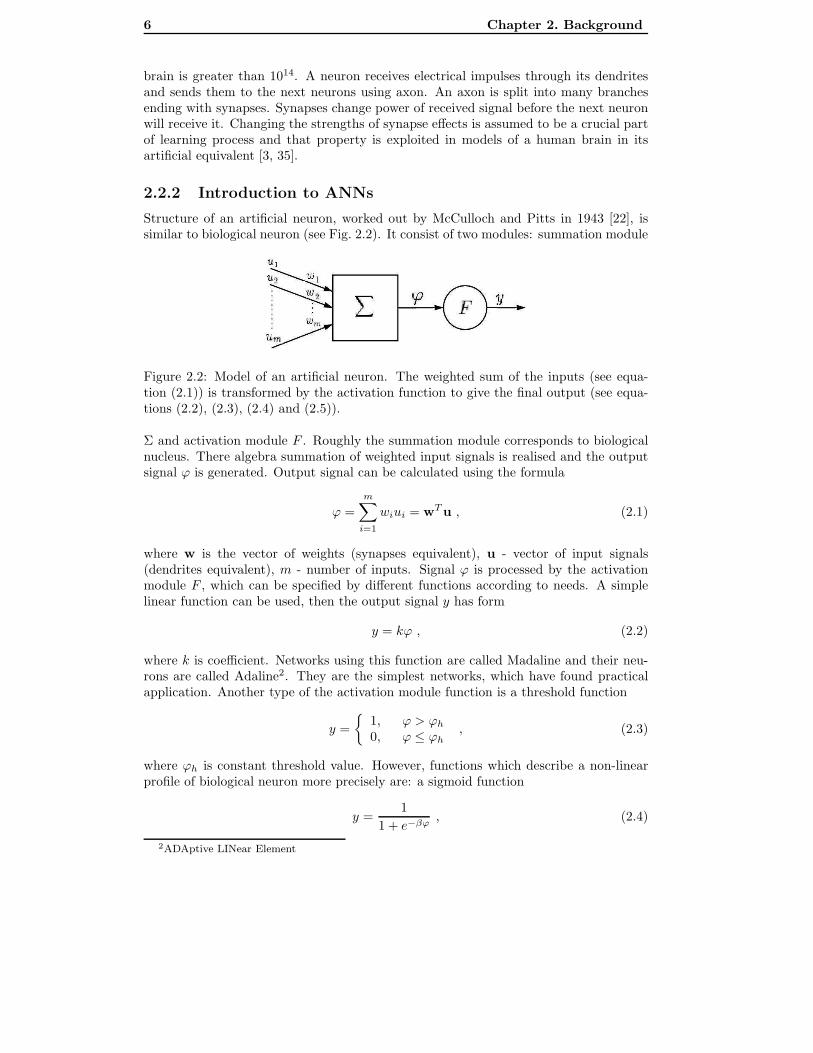
Structure of an artificial neuron, worked out by McCulloch and Pitts in 1943 [22], issimilar to biological neuron (see Fig. 2.2). It consist of two modules: summation module

Figure 2.2: Model of an artificial neuron. The weighted sum of the inputs (see equa-tion (2.1)) is transformed by the activation function to give the final output (see equa-tions (2.2), (2.3), (2.4) and (2.5)).

Σ and activation module F . Roughly the summation module corresponds to biologicalnucleus. There algebra summation of weighted input signals is realised and the outputsignal ϕ is generated. Output signal can be calculated using the formula

ϕ =

m∑

i=1

wiui = wT u , (2.1)

where w is the vector of weights (synapses equivalent), u - vector of input signals(dendrites equivalent), m - number of inputs. Signal ϕ is processed by the activationmodule F , which can be specified by different functions according to needs. A simplelinear function can be used, then the output signal y has form

y = kϕ , (2.2)

where k is coefficient. Networks using this function are called Madaline and their neu-rons are called Adaline2. They are the simplest networks, which have found practicalapplication. Another type of the activation module function is a threshold function

y =

{

1, ϕ > ϕh

0, ϕ ≤ ϕh, (2.3)

where ϕh is constant threshold value. However, functions which describe a non-linearprofile of biological neuron more precisely are: a sigmoid function

y =1

1 + e−βϕ, (2.4)

2ADAptive LINear Element

2.2. Neural networks 7

where β is given parameter and a tangensoid function

y = tanh(αϕ

2)1 − e−αϕ

1 + e−αϕ, (2.5)

where α is given parameter [3, 35, 37].

Information capacity and processing ability of a single neuron is relatively small.However, it can be raised by the appropriate connection of many neurons. In 1958the first ANN, called perceptron, was developed by Rosenblatt [31]. It was used foralphanumerical character recognition. Although the results were not satisfactory (prob-lems appeared when characters were more complex or the scale was changed) it wassuccessful as the first system built, which simulated a neural network. Rosenblatt hasalso proved that if a given problem can be solved by a perceptron, then the solution canbe found in a finite number of steps [3, 35, 37].

After publication of the book “Perceptrons” by Minsky and Papert in 1969 [24]research in the area of ANNs had come to a standstill. The authors proved that percep-trons cannot solve linearly non-separable problems (e.g. compute an XOR-function).Research has been resumed after almost 15 years by a series of publications showingthat these limitations are not applicable to non-linear multilayer networks. Effectivelearning methods have also been introduced [3, 35, 37].

Neurons in the multilayer ANNs are grouped into three different types of layers:input, output, and hidden layer (see Fig. 2.3). There can be one or more hidden layers

Figure 2.3: Multilayer feed-forward ANN. From the neurons in the input layer (IL)signals are propagated to the hidden layer (HL) and then finally to the output layer(OL).

in the network but only one output and one input layer. The number of neurons in theinput layer is specified by the type and amount of data which will be given to the input.The number of output neurons corresponds to the type of answer of the network. Theamount of hidden layers and their neurons is more difficult to determine. A networkwith one hidden layer suffices to solve most tasks. None of the known problems needs anetwork with more than three hidden layers in order to be solved (see Fig. 2.4). Thereis no good recipe for the number of hidden neurons selection. One of the methods isdescribed by formula

Nh =√

NiNo , (2.6)

8 Chapter 2. Background

Figure 2.4: Selection of the number of layers for solving different problems. Morecomplicated networks can solve more complicated issues.

where Nh is the number of neurons in the hidden layer, and Ni and No are the corre-sponding numbers for the input and output layers, respectively. However, usually thequantity of hidden neurons is determined empirically [3, 35, 37].

Two types of a multilayer ANNs can be distinguished with regards to the archi-tecture: feed-forward and feedback networks. In the feed-forward networks signal canmove in one direction only and cannot move between neurons in the same layer (seeFig. 2.3). Such networks can be used in the pattern recognition. Feedback networks aremore complicated, because a signal can be sent back to the input of the same layer witha changed value (see Fig. 2.5). Signals can move in these loops until the proper state isachieved. These networks are also called interactive or recurrent [35, 1].

Figure 2.5: Multilayer feedback ANN. A signal can be returned to the same layer toadjust the proper state.

2.2. Neural networks 9

2.2.3 Training of the ANN

The process of training of the ANN consists in changing the weights assigned to connec-tions of neurons until the achieved result is satisfactory. Two main kinds of learning canbe distinguished: supervised and unsupervised learning. In the first of them externalteacher is being used to correct the answers given by the network. ANN is consideredto have learned when computed errors are minimized. Unsupervised learning does notuse a teacher. ANN has to distinguish patterns using the information given to theinput without external help. This learning method is also called self-organisation. Itworks like a brain which uses sensory impressions to recognise the world without anyinstructions [3, 35].

One of the best known learning algorithms is the Back-Propagation Algorithm (BPA).This basic, supervised learning algorithm for multilayered feed-forward networks gives arecipe for changing the weights of the elements in neighbouring layers. It consists in min-imization of the sum-of-squares errors, known as least squares. Despite of the fact thatBPA is an ill-conditioned optimization problem [12], thanks to specific way of the errorspropagation, BPA has become one of the most effective learning algorithms [3, 35, 37].

To teach ANN using BPA the following steps have to be carried out for each patternin the learning set:

1. Insert the learning vector uµ as an input to the network.

2. Evaluate the output values umµj of each element for all layers using the formula

umµj = f(ϕmµ

j ) = f(

nm−1∑

i=0

wmji u

(m−1)µi ) . (2.7)

3. Evaluate error values δMµj for the output layer using the formula

δMµj = f ′(ϕMµ

j )δµj = f ′(ϕMµ

j )(yzµj − yµ

j ) . (2.8)

4. Evaluate sum-of-squares errors ξµ from

ξµ =1

2

n∑

j=1

(δµj )2 . (2.9)

5. Carry out the back-propagation of output layer error δMµj to all elements of hidden

layers (see Fig. 2.6) calculating their errors δmµj from

δmµj = f ′(ϕmµ

j )

nm+1∑

l=1

δ(m+1)µl w

(m+1)lj . (2.10)

6. Update the weights of all elements between output and hidden layers and thenbetween all hidden layers moving towards the input layer. Changes of the weightscan be obtained from

∆µwmji = ηδmµ

j u(m−1)µi . (2.11)

10 Chapter 2. Background

Figure 2.6: Back-propagation of errors values.

Above steps have to be repeated until satisfactory minimum of complete error functionis achieved:

ξ =

P∑

µ=1

ξµ =1

2

P∑

µ=1

n∑

j=1

(yzµj − ϕµ

j )2 , (2.12)

where the symbols used in equations (2.7), (2.8), (2.9), (2.10), (2.11) and (2.12) denote:P - number of learning patterns,µ - index of actual learning pattern, µ = 1, . . . , P ,M - number of layers (input layer is not included),m - index of actual layer, m = 1, . . . , M ,nm - number of elements (neurons) in layer m,j - index of actual element, j = 1, . . . , nm,ϕµ

j - weighted sum of input values for element j in layer µ,

f - activation function (see equations (2.2), (2.3), (2.4) and (2.5)),wm

ji - weight between element j in layer m and element i in layer m − 1,

u(m−1)µi - output of element i in layer m − 1 for pattern µ,

δµj - learning error for element j for pattern µ,

yzµj - expected network output value for element j for pattern µ,

yµj - actual network output value for element j for pattern µ,

∆µwmji - change of given weight for pattern µ,

η - proportion coefficient.

Every iteration of these instructions is called epoch. After the learning process isfinished another set of patterns can be used to verify the knowledge of the ANN. Forcomplicated networks and large sets of patterns the learning procedure can take a lot oftime. Usually it is necessary to repeat the learning process many times with differentcoefficients selected by trial and error [3, 35, 37].

There is a variety of optimisation methods which can be used to accelerate thelearning process. One of them is momentum technique [25], which consists in calculatingthe changes of the weights for the pattern (k + 1) using formula

∆µwmji (k + 1) = ηδmµ

j u(m−1)µi + α∆µwm

ji (k) (2.13)

where α is constant value which determines the influence of the previous change ofweights to the current change. This equation is more complex version of equation (2.11).

2.3. Support Vector Machines 11

2.3 Support Vector Machines

SVM proposed by Vapnik [6, 39, 40, 41] was originally designed for classification andregression tasks, however later has expanded in another directions [34]. Essence of SVMmethod is construction of optimal hyperplane, which can separate data from oppositeclasses using the biggest possible margin. Margin is a distance between optimal hyper-plane and a vector which lies closest to it. An example of such hyperplane is illustratedon figure 2.7. As it can be seen on the drawing, there can be many hyperplanes which

Figure 2.7: Optimal hyperplane separating two classes.

can separate two classes, but with regard to optimal choice, the most interesting solu-tion can be obtained by gaining the biggest possible margin. Optimal hyperplane shouldsatisfy

ykF (xk)

||w||≥ τ k = 1, 2, ..., n, (2.14)

where τ is a margin and F (x) is defined as:

F (x) = wT x + b . (2.15)

As we have mentioned in section 2.2.2, this function is not suitable for solving morecomplicated, linearly non-separable problems [32, 34, 21, 36].

2.3.1 Kernel functions

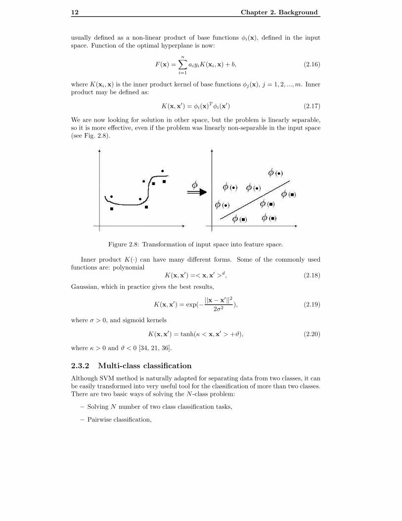
Possibility of occurrence of the linearly non-separability in the input space consist thecause why the idea of SVM is not optimal for hyperplane construction in the inputspace but rather in high-dimensional so called feature space Z. The feature space is

12 Chapter 2. Background

usually defined as a non-linear product of base functions φi(x), defined in the inputspace. Function of the optimal hyperplane is now:

F (x) =

n∑

i=1

aiyiK(xi,x) + b, (2.16)

where K(xi,x) is the inner product kernel of base functions φj(x), j = 1, 2, ..., m. Innerproduct may be defined as:

K(x,x′) = φi(x)T φi(x′) (2.17)

We are now looking for solution in other space, but the problem is linearly separable,so it is more effective, even if the problem was linearly non-separable in the input space(see Fig. 2.8).

Figure 2.8: Transformation of input space into feature space.

Inner product K(·) can have many different forms. Some of the commonly usedfunctions are: polynomial

K(x,x′) =< x,x′ >d, (2.18)

Gaussian, which in practice gives the best results,

K(x,x′) = exp(−||x − x′||2

2σ2), (2.19)

where σ > 0, and sigmoid kernels

K(x,x′) = tanh(κ < x,x′ > +ϑ), (2.20)

where κ > 0 and ϑ < 0 [34, 21, 36].

2.3.2 Multi-class classification

Although SVM method is naturally adapted for separating data from two classes, it canbe easily transformed into very useful tool for the classification of more than two classes.There are two basic ways of solving the N -class problem:

– Solving N number of two class classification tasks,

– Pairwise classification,

2.3. Support Vector Machines 13

The first method consists in teaching of many classifiers using one versus the restmethod. It means that while solving every i-th task (i = 1, 2, ..., N) we carry out theseparation of one, current class from the other classes and every time new hyperplanecomes into being

y(x; wi, bi) = wTi x + bi = 0. (2.21)

Support vectors, which belong to class i satisfy y(x; wi, bi) = 1, whereas the other onessatisfy condition y(x; wi, bi) = −1. If for a new vector we have

y(x; wi, bi) > 0, (2.22)

then the vector is assigned for class i. However, it may happen, that (2.22) is true formany i or is not true for any of them. For such cases the classification is unfeasible [34,36].

In pairwise classification N -class problem is replaced with N(N−1)/2 differentiationtasks between two classes. However, the number of classifiers is greater than in the pre-vious method, individual classifiers can be trained faster and depending on the datasetthis results in time savings [34]. Unambiguous classification is not always possible, sinceit may happen that more than one class will get the same number of votes [36]. Solutionof that problem is described in [28].

14 Chapter 2. Background

Chapter 3

Approach

3.1 Recognition of skin diseases

Dermatology is considered to be heavily dependent on visual estimations. Even veryexperienced doctors have to continually verify their knowledge. The changes of the skinare visible but they are hard to identify because of the large number of different skindiseases, which have similar or identical symptoms.

“Dermatology is different from other specialties because the diseases caneasily be seen. Keen eyes, aided sometimes by a magnifying glass, are allthat are needed for a complete examination of the skin. Often it is best toexamine the patient briefly before obtaining a full history. A quick look willprompt the right questions” [19, p.35].

As it was shown in the chapter 2, ANNs and SVM are very powerful tools for patternrecognition, which extent the role of magnifying glass in the smart way. During di-agnosis of skin diseases, the image of the skin fragment has to be inspected. To helpdermatologists with the diagnosis we developed the Skinchecker system.

3.2 Chosen diseases

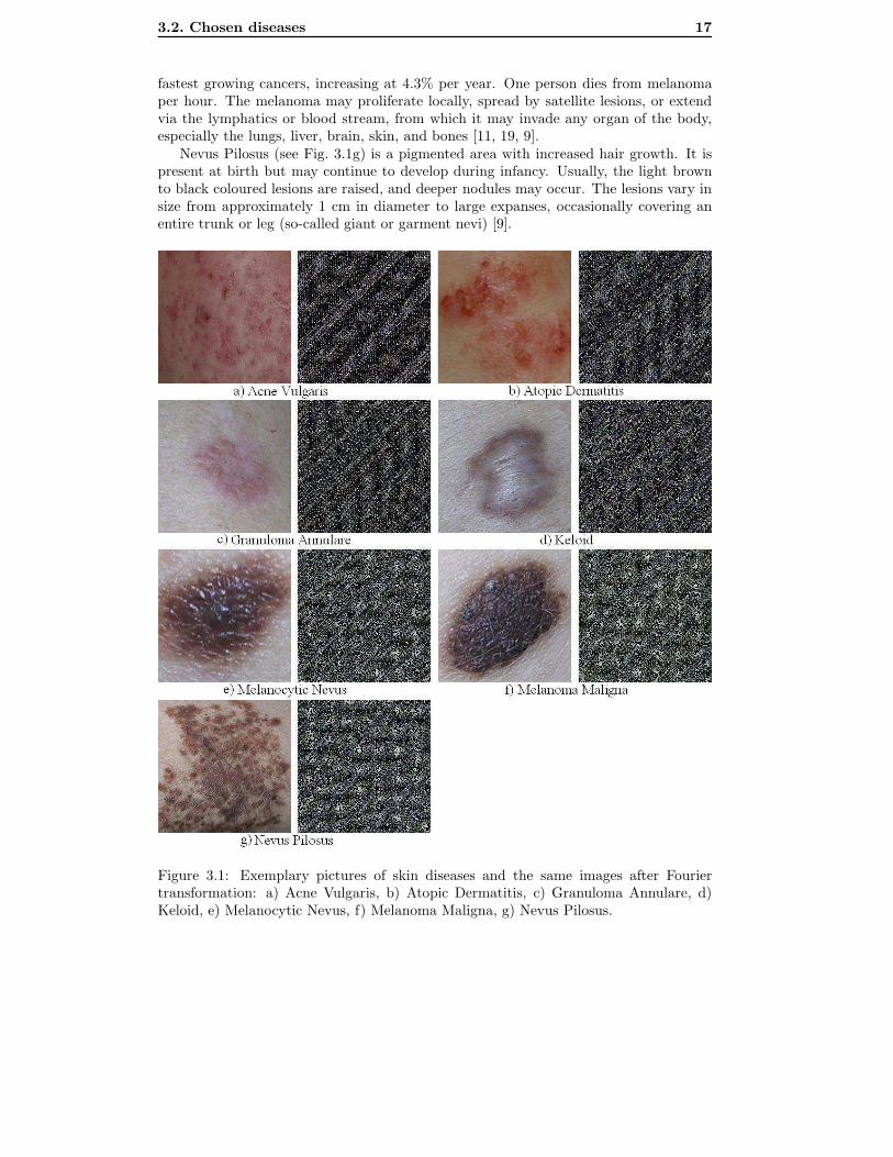
From among 789 dermatological pictures received from professor Ryszard Zaba from theDermatological Clinic of Poznan University of Medical Sciences we have chosen 215 withbest quality and best applicability in pattern recognition area. Those pictures represent7 different diseases (see Fig. 3.1) which are shortly described in this section. Numbersof pictures available for each of chosen diseases are presented in the table 3.1.

Acne Vulgaris (see Fig. 3.1a) is a chronic inflammatory disease characterized bycysts, open and closed comedones (plugged lesions containing a “cottage-cheese” likematerial), pus pockets, and raised red swellings. Often occurs in puberty, though mayoccur in the 20s or 30s. Several factors are involved in the pathogenesis: inheritance,increased sebum production, an abnormality of the microbial flora, cornification of thepilosebaceous duct and the production of inflammation [11, 19, 9].

Atopic1 Dermatitis (see Fig. 3.1b), also known as Eczema, is generally attributed toa malfunction in the body’s immune system. It tends to occur in people who have a

1Greek: a-topos - without a place.

15

16 Chapter 3. Approach

Disease Number of picturesAcne Vulgaris 29Atopic Dermatitis 29Granuloma Annulare 19Keloid 29Melanocytic Nevus 75Melanoma Maligna 13Nevus Pilosus 21

Table 3.1: Diseases chosen for training the system.

family history of allergies. Many children who get this disease outgrow it at puberty,but later develop dermatitis of the hands as adults. Risk factors may include exposureto tobacco smoke, skin infections, changes in climate, irritating chemicals, food allergies,and stress. It is manifested by lichenification, excoriation, and crusting involving mainlythe face, neck and the flexural surfaces of the elbow and knee. The clinical picturevaries greatly depending on the age of the patient, the course and duration of thedisease. Atopic eczema may be distinguished from other types of dermatitis because ofits typical course and associated stigmata. About 15% of the population has at leastone atopic manifestation and its prevalence is rising [11, 19, 9].

Granuloma Annulare (see Fig. 3.1c) is characterized by a ring composed of smooth,firm papules or nodules on the skin which gradually enlarges. Multiple lesions maybe present. In the generalized form, multiple small skin-coloured, erythematous orviolaceous lesions appear in a symmetrical fashion on the trunk and, to a lesser extent,on the limbs, and the distinctive annular pattern is not always present [9].

Keloid (see Fig. 3.1d) is an excessive connective tissue response to skin injury char-acterized by firm red or pink plaques extending beyond the area of the original wound.They are most frequently found over the upper trunk and upper arms. Keloids aremore common in darkly pigmented individuals, and most cases have been reported inpatients between the ages of 10 and 30. There is a familial tendency to keloid formation.Normally, when the skin is cut, the cells of the underlying connective tissue rush in torepair the area by forming a collagen-based scar. Under normal circumstances, the cellsknow at what point they should stop making scar tissue. However, in some geneticallypredisposed individuals, the cells do not stop when they are supposed to, causing excessheavy scar tissue to form. Treatment of keloids is difficult, and as of now, the besttreatment is prevention [11, 19, 9].

Melanocytic Nevus (see Fig. 3.1e) is some of the most common growth that occurson the skin. Melanocytic nevi can be present at birth or around the time of birth.These tend to be larger moles and are referred to as congenital nevi. During childhood“regular moles” may begin to appear. Typically they are skin color to dark brown, flatto dome shaped growths that can appear anywhere on the skin. They are harmless, butsometimes they can be difficult to tell from skin cancer by lay persons. This can beespecially true for a type of mole called a dysplastic nevus. Any growth that suddenlychanges in size, color, shape, bleeds, itches on a regular basis or becomes inflamed orirritated needs to be evaluated by a dermatologist [23, 19].

Melanoma Malignas (see Fig. 3.1f) is a type of skin cancer that originates in themelanocytes, the skin cells containing pigment or color scattered throughout the body.In the United States alone, 32000 people are affected per year. Melanoma is one of the

3.2. Chosen diseases 17

fastest growing cancers, increasing at 4.3% per year. One person dies from melanomaper hour. The melanoma may proliferate locally, spread by satellite lesions, or extendvia the lymphatics or blood stream, from which it may invade any organ of the body,especially the lungs, liver, brain, skin, and bones [11, 19, 9].

Nevus Pilosus (see Fig. 3.1g) is a pigmented area with increased hair growth. It ispresent at birth but may continue to develop during infancy. Usually, the light brownto black coloured lesions are raised, and deeper nodules may occur. The lesions vary insize from approximately 1 cm in diameter to large expanses, occasionally covering anentire trunk or leg (so-called giant or garment nevi) [9].

Figure 3.1: Exemplary pictures of skin diseases and the same images after Fouriertransformation: a) Acne Vulgaris, b) Atopic Dermatitis, c) Granuloma Annulare, d)Keloid, e) Melanocytic Nevus, f) Melanoma Maligna, g) Nevus Pilosus.

18 Chapter 3. Approach

3.3 Dataset

Before training programs can be used, all the pictures have to be compiled into properdataset file. We have developed the Skinchecker-DataSet module (see Fig. 3.2) whichprovides all necessary, for our purposes, tools for image preprocessing. It also simplifiesthe organization of lists of all diseases and their images. User can simply add newdiseases and assign pictures to them as well as remove any not used data. All listscan be saved and used in future, what is very useful when there is a need to prepare adataset from the same collection of pictures but with another parameters or when someimages need to be added to the list.

Figure 3.2: Interface of Skinchecker-DataSet module. It builds dataset files from imagesof different diseases given in the list.

When the list of diseases and their images is ready, some options should be alsoset. First of all, user should decide if the dataset will be used for ANN or SVM versionof Skinchecker, because training files differ slightly between two versions. User canalso choose whether images will be ordered in the dataset file as they are in the list ofimages or if they should be compiled randomly, what can be significant for some learningalgorithms. Fourier or Wavelet transforms can be also performed on pictures, what isexplained in section 3.3.1. There is also an option to save images which were previouslytransformed. After clicking “Create data set” button dataset file will be created. Thatfile can be then used by ANN or SVM version of Skinchecker training module.

3.4. Skinchecker with ANN 19

3.3.1 Image preprocessing

After some trials with training using whole images were made, it appeared that there isa need to perform some additional image preprocessing. First tests took large amountof time and were not effective, because of large input vectors (n2 input neurons for n×npictures). The total network error could not go below 0,3. The situation has changedafter performing Fourier transform [29] (see Fig. 3.1). After taking the average valueof diagonal lines of pixels from transformed images we have obtained spectrum, whichwe have used as a pattern for recognition (2n input neurons for n × n pictures). Suchsystem can be trained in reasonable time and gives satisfactory results. However, thereis also a limitation, because of Fast Fourier Transform (FFT) algorithm requirementsthe size of an image must be power of 2 [29]. We have used 256 × 256 pictures, thereforethe number of input neurons is 512.

3.4 Skinchecker with ANN

This version of Skinchecker uses Fast Artificial Neural Network Library (FANN) tocreate and train the network. FANN is a free open source neural network library, whichimplements multilayer artificial neural networks in C [26].

In our tests we have used 2 algorithms from among those available in FANN: quick-prop and incremental. The best results have been achieved for incremental algorithm,which is standard backpropagation algorithm, where the weights are updated manytimes during a single epoch. We have build ANN with 512 neurons in the input layer,7 in the output layer and 12 in the hidden layer. Results of testing the network arepresented in the next chapter.

3.5 Skinchecker with SVM

This version of Skinchecker uses LIBSVM library [8], which provides the support vectorclassification (SVC) in two versions: C-SVC and ν-SVC. After using the C-SVC methodit has appeared that results were not satisfactory. Therefore we have decided to use ν-SVC and we have obtained satisfactory results for ν < 0, 3 (presented in next chapter).More information about above mentioned SVC methods can be found in [8, 36].

20 Chapter 3. Approach

Chapter 4

Results

4.1 Results for ANN

We used method described in the chapter 3. We have built the 3-layers ANN with 512inputs, 7 outputs and 12 neurons in hidden layer. In this section results of testing thatANN are presented.

4.1.1 Quickprop algorithm

While training the network, we have set the desired total network error to 0,001. Wehave set also the maximum number of epochs to 3000. Unfortunately it was impossiblefor quickprop algorithm to achieve that error, however obtained values are near thosedesired. They vary between 0,003 and 0,005 according to the momentum value. TheFig. 4.1 presents how the learning proceeded. It shows the total network error in con-secutive epochs. We can see that the best error flow was for α = 0, 5, it is near theperfect desired flow.

Disease NoP α = 0, 2 α = 0, 4 α = 0, 5 α = 0, 6 α = 0, 7Acne Vulgaris 29 93,6% 96,0% 94,4% 95,2% 96,0%Atopic Dermatitis 29 95,3% 94,0% 95,3% 96,0% 93,6%Granuloma Annulare 19 94,4% 94,3% 93,4% 95,2% 93,9%Keloid 29 95,2% 94,5% 95,0% 94,7% 94,1%Melanocytic Nevus 75 96,7% 97,5% 97,0% 96,4% 96,0%Melanoma Maligna 13 95,4% 94,3% 92,0% 93,0% 93,6%Nevus Pilosus 21 95,1% 94,9% 95,5% 95,9% 94,1%Total 215 95,1% 95,1% 94,7% 95,2% 94,5%

Table 4.1: Results of testing the ANN with quickprop algorithm for different momentumvalues. NoP - number of pictures used for training the ANN.

21

22 Chapter 4. Results

Figure 4.1: Training the ANN using quickprop algorithm. The chart presents totalnetwork error through epochs for different momentum values.

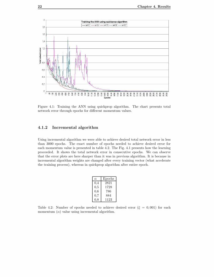
4.1.2 Incremental algorithm

Using incremental algorithm we were able to achieve desired total network error in lessthan 3000 epochs. The exact number of epochs needed to achieve desired error foreach momentum value is presented in table 4.2. The Fig. 4.1 presents how the learningproceeded. It shows the total network error in consecutive epochs. We can observethat the error plots are here sharper than it was in previous algorithm. It is because inincremental algorithm weights are changed after every training vector (what acceleratethe training process), whereas in quickprop algorithm after entire epoch.

α Epochs0,4 28210,5 17280,6 7860,7 8840,8 1123

Table 4.2: Number of epochs needed to achieve desired error (ξ = 0, 001) for eachmomentum (α) value using incremental algorithm.

4.2. Results for SVM 23

Figure 4.2: Training the ANN using incremental algorithm. The chart presents totalnetwork error through epochs for different momentum values.

Disease NoP α = 0, 4 α = 0, 5 α = 0, 6 α = 0, 7 α = 0, 8Acne Vulgaris 29 96,7% 97,4% 98,9% 98,4% 99,6%Atopic Dermatitis 29 99,8% 98,6% 99,2% 99,0% 99,9%Granuloma Annulare 19 95,0% 96,6% 96,6% 96,4% 99,8%Keloid 29 99,8% 97,4% 96,1% 96,8% 99,8%Melanocytic Nevus 75 99,4% 98,7% 99,9% 99,0% 99,8%Melanoma Maligna 13 98,1% 97,7% 98,7% 97,3% 97,6%Nevus Pilosus 21 98,9% 99,8% 99,2% 98,7% 95,5%Total 215 98,2% 98,0% 98,4% 97,9% 98,9%

Table 4.3: Results of testing the ANN with incremental algorithm for different momen-tum values. NoP - number of pictures used for training the ANN.

4.2 Results for SVM

We have used ν-SVC for classification of pictures, as it was outlined in chapter 3. Theresults of testing the SVM for different ν value are presented in the table 4.4. Results forMelanoma Maligna are much worse comparing to other diseases: partially because it’sthe smallest training set but also because those pictures are quite similar to MelanocyticNevus, which is the biggest set. This is also a common problem in dermatology todifferentiate between Melanocytic Nevus which is not very dangerous and MelanomaMaligna which can be lethal.

24 Chapter 4. Results

Disease NoP ν = 0, 05 ν = 0, 1 ν = 0, 15 ν = 0, 2 ν = 0, 25Acne Vulgaris 29 89,3% 89,9% 89,4% 89,6% 89,5%Atopic Dermatitis 29 84,2% 85,0% 84,8% 84,9% 84,8%Granuloma Annulare 19 91,3% 90,8% 90,7% 90,9% 90,8%Keloid 29 92,5% 92,9% 93,0% 93,0% 92,7%Melanocytic Nevus 75 89,1% 89,4% 89,6% 87,2% 82,3%Melanoma Maligna 13 57,3% 58,1% 60,4% 43,2% 18,9%Nevus Pilosus 21 88,9% 90,1% 90,0% 90,1% 91,7%Total 215 84,7% 85,2% 85,4% 82,7% 78,7%

Table 4.4: Results of testing the SVM with ν-SVC for different ν values. NoP - numberof pictures used for training the SVM.

4.3 Comparison

The Fig. 4.3 presents a comparison of the best results achieved by each method. Itappears that much better results in classification were obtained using ANN than SVM.It seems also that ANNs are more resistant to insufficient data amount, because evenfor small set of Melanoma Maligna pictures results were satisfactory. That cannot besaid about SVM, which had a problem with classification of above mentioned diseaseand mislead it with Melanocytic Nevus.

Figure 4.3: Comparison of results.

Comparing both used ANN’s algorithms we can observe that better results wereobtained using incremental algorithm than quickprop algorithm. However, it can changewhen bigger, more complicated datasets will be used. Incremental algorithm is faster,but if there will be more diseases to classify it may appear that quickprop algorithmwill be more effective.

4.4. Cross validation testing 25

4.4 Cross validation testing

We have used holdout method to perform the cross validation. From all 215 pictureswe have randomly selected 129 (60%) for training and 86 (40%) for validation. Resultsare presented in the table 4.5. We can observe that changes in ANN’s results are notsignificant, whereas SVM’s accuracy has decreased over 30%.

SVM ANNDisease TS VS ν = 0, 15 TS VS Quick IncrAcne Vulgaris 16 13 45,1% 15 14 96,1% 99,6%Atopic Dermatitis 20 9 42,1% 20 9 96,3% 100%Granuloma Annulare 15 4 42,9% 15 4 94,0% 98,7%Keloid 18 11 55,0% 18 11 95,4% 97,2%Melanocytic Nevus 38 37 64,1% 45 30 97,4% 99,5%Melanoma Maligna 9 4 48,4% 7 6 96,8% 97,5%Nevus Pilosus 13 8 66,1% 9 12 97,4% 100%Total 129 86 52,0% 129 86 96,2% 98,9%

Table 4.5: Results of testing the SVM and ANN using cross validation. TS - number ofsamples used for training, VS - number of samples used for validation, Quick - resultsfor quickprop algorithm with α = 0, 5, Incr - results for incremental algorithm withα = 0, 8.

26 Chapter 4. Results

Chapter 5

Conclusions

ANNs are very efficient tools for pattern recognition and they can be successfully used indermatological applications. They can increase the detectability of dangerous diseasesand lower the mortality rate of patients. Skinchecker can recognize diseases but thedoctor has to decide if there is a need to analyse some part of the skin. After using theprogram, the doctor has to decide what to do with the results. The data obtained fromthe program can be helpful. Although computers cannot replace the dermatologist, theycan make his work easier and more effective. Proposed system might be also very usefulfor general practicioners, who do not have wide knowledge about dermatology.

5.1 Limitations

Currently Skinchecker can be used only on Windows platform, it was tested on WindowsXP. However it can be easily transfered to any other platform supported by FANN libraryor LIBSVM.

5.2 Future work

Although Skinchecker has classified diseases correctly, there are still a lot of improve-ments which can be done to increase its accuracy. Some additional information can beadded to the training set, for example age of the patient, colour of the skin, etc. Biggerdatasets with more different diseases should be used to make the use of Skincheckerreasonable, however it is hard to obtain enough pictures currently. Also a tool, whichwill help the doctor to prepare the picture for classification would be desirable, as wellas some hardware to obtain proper images of the skin. Set of instructions about howto take usable pictures, including information about light, distance from a patient, etc.should improve the usability of Skinchecker.

27

28 Chapter 5. Conclusions

Chapter 6

Acknowledgements

I would like to thank Michael Minock from Umea University and Micha l Mucha fromAdam Mickiewicz University in Poznan for ideas and help with realisation of this project.I would also like to thank professor Ryszard Zaba from the Dermatological Clinic ofPoznan University of Medical Sciences for dermatological pictures and for all medicaladvices. Many thanks to Asim Sheikh for checking my english. Also to Per Lindstromfor his help during my study period in Umea and Jurgen Borstler for teaching me howto write publications.

29

30 Chapter 6. Acknowledgements

References

[1] S. Agatonovic-Kustrin and R. Beresford. Basic concepts of artificial neural net-work (ANN) modeling and its application in pharmaceutical research. Journal ofPharmaceutical and Biomedical Analysis, 22:717–727, 2000.

[2] Micha l Antkowiak. Recognition of skin diseases using artificial neural networks. InProceeding of USCCS’05, pages 313–325, 2005.

[3] Chris M. Bishop. Neural networks and their applications. Review of ScientificInstruments, 65(6):1803–1832, 1994.

[4] Chris M. Bishop. Neural Networks for Pattern Recognition. Clarendon Press, Ox-ford, UK, 1995.

[5] A. Blum, H. Luedtke, U. Ellwanger, R. Schwabe, G. Rassner, and C. Garbe. Dig-ital image analysis for diagnosis of cutaneous melanoma. development of a highlyeffective computer algorithm based on analysis of 837 melanocytic lesions. BritishJournal of Dermatology, 151:1029–1038, 2004.

[6] B. E. Boser, I. M. Guyon, and V. N. Vapnik. A training algorithm for optimalmargin classifier. In 5th Annual ACM Workshop on COLT, pages 144–152, 1992.

[7] Canfield Scientific. Home Page. http://www.canfieldsci.com, accessed April 27,2005, 2005.

[8] Chih-Chung Chang and Chih-Jen Lin. LIBSVM: a Library for Support VectorMachines, 2001. http://www.csie.ntu.edu.tw/ cjlin/libsvm.

[9] DermIS. Dermatology Information Service. http://www.dermis.net/, accessedMarch 30, 2006, 2006.

[10] Anthony du Vivier. Atlas of Clinical Dermatology. Churchill Livingstone, 2002.

[11] eCureMe. Medical Dictionary. http://www.ecureme.com/, accessed March 30,2006, 2006.

[12] Jerry Eriksson, Marten Gulliksson, Per Lindstrom, and Per-Ake Wedin. Regu-larization tools for training large feed-forward neural networks using automaticdifferentation. Optimization Methods and Software, 10:49–69, 1998.

[13] Monika Gniadecka, Peter Alshede Philipsen, Sigurdur Sigurdsson, Sonja Wessel,and et al. Melanoma diagnosis by Raman spectroscopy and neural networks: Struc-ture alterations in proteins and lipids in intact cancer tissue. J Invest Dermatol,122:443–449, 2004.

31

32 REFERENCES

[14] David Delgado Gomez, Toke Koldborg Jensen, Sune Darkner, andJens Michael Carstensen. Automated visual scoring of psoriasis.http://www.imm.dtu.dk/visiondag/VD02/medicinsk/articulo.pdf, 2002.

[15] H. A. Guvenir and N. Emeksiz. An expert system for the differential diagnosis oferythemato-squamous diseases. Expert Systems with Applications, 18:43–49, 2000.

[16] H. Handels, Th. Roß, J. Kreusch, H. H. Wolff, and S. J. Poppl. Feature selection foroptimized skin tumor recognition using genetic algorithms. Artificial Intelligencein Medicine, 16:283–297, 1999.

[17] K. Hoffmann, T. Gambichler, A. Rick, M. Kreutz, and et al. Diagnostic and neu-ral analysis of skin cancer (DANAOS). A multicentre study for collection andcomputer-aided analysis of data from pigmented skin lesions using digital der-moscopy. British Journal of Dermatology, 149:801–809, 2003.

[18] Ming Huang and Vojislav Kecman. Gene extraction for cancer diagnosis by supportvector machines. Artificial Intelligence in Medicine, 35:185–194, 2005.

[19] J. A. A. Hunter, J. A. Savin, and M. V. Dahl. Clinical Dermatology. BlackwellScience, 1995.

[20] Dipti Itchhaporia, Peter B. Snoe, Robert J. Almassy, and William J. Oetgen. Artifi-cial neural networks: Current status in cardiovascular medicine. J Am Coll Cardiol,28(2):515–521, 1996.

[21] Norbert Jankowski. Ontogeniczne sieci neuronowe. Akademicka OficynaWydawnicza EXIT, Warszawa, PL, 2003.

[22] W. S. McCulloch and W. H. Pitts. A logical calculus of the ideas immanent innervous activity. Bulletin of Mathematical Biophysics, 5:115–133, 1943.

[23] John L. Meisenheimer. Melanocytic Nevus. http://www.orlandoskindoc.com, ac-cessed March 30, 2006, 2006.

[24] M. Minsky and S. Papert. Perceptrons. Cambridge, Mass.: MIT Press, 1969.

[25] M. Moreira and E. Fiesler. Neural networks with adaptive learning rate and momen-tum terms. Technical Report 95-04, Institut Dalle Morre D’Intelligence ArtificiellePerceptive, Martigny, Valais, Switzerland, 1995.

[26] Steffen Nissen. Implementation of a fast artificial neural network library (fann).Technical report, Department of Computer Science University of Copenhagen,Copenhagen, DK, 2003.

[27] D. Piccolo, A. Ferrari, K. Peris, R. Daidone, B. Ruggeri, and S. Chimenti. Der-moscopic diagnosis by a trained clinician vs. a clinician with minimal dermoscopytraining vs. computer-aided diagnosis of 341 pigmented skin lesions: a comparativestudy. British Journal of Dermatology, 147:481–486, 2002.

[28] J. C. Platt, N. Christianini, and J. Shave-Taylor. Large margin dags for multiclassclassification. In Advances in Neural Information Processing Systems, pages 547–553, 2000.

REFERENCES 33

[29] William H. Press, Saul A. Teukolsky, William T. Vetterling, and Brian P. Flannery.Numerical Recipes in C: The Art of Scientific Computing. Cambridge UniversityPress, Cambridge, UK, 1992.

[30] Brian D. Ripley. Pattern Recognition and Neural Networks. Cambridge UniversityPress, Cambridge, UK, 1996.

[31] F. Rosenblatt. The perceptron: a probabilistic model for information storage andorganization in the brain. Psychological Review, 65:386–408, 1958.

[32] Bernhard Sholkopf. Statistical learning and kernel methods. Technical ReportMSR-TR-2000-23, Microsoft Research Limited, Cambridge, UK, 2000.

[33] Bernhard Sholkopf. Survival-time classification of breast cancer patients. Techni-cal Report 01-03, National Taiwan University of Science and Technology, Taipei,Taiwan, 2001.

[34] Bernhard Sholkopf and Alex Smola. Learning with Kernels. MIT Press, Cambridge,MA, 2002.

[35] Christos Stergiou and Dimitrios Siganos. Neural networks. SURPRISE 96 Journal,4, 1996.

[36] Piotr Szczepaniak. Obliczenia inteligentne, szybkie przekszta lcenia i klasyfikatory.Akademicka Oficyna Wydawnicza EXIT, Warszawa, PL, 2004.

[37] Ryszard Tadeusiewicz. Sieci neuronowe (Neural Networks). Akademicka OficynaWydawnicza, Warszawa, PL, 1993.

[38] Andrew Tomlinson. Medical applications for pattern classifiers and image process-ing. http://www.railwaybridge.co.uk, accessed April 27, 2005, 2000.

[39] V. Vapnik. The Nature of Statistical Learning Theory. Springer-Verlag, New York,USA, 1995.

[40] V. Vapnik. Statistical Learning Theory. Wiley, New York, USA, 1998.

[41] V. Vapnik. The support vector method of function estimation. Neural Networksand Machine Learning, pages 239–268, 1998.

[42] World Health Organisation. Ultraviolet radiation and the INTERSUN Programme.http://www.who.int, accessed April 27, 2005, 2005.

34 REFERENCES

Appendix A

Back-Propagation Learning

Algorithm description

A.1 Training

for each layer (except input layer):

for each neuron in layer:

for each weight of neuron:

set random weight;

while total network error is greater than 0.01:

for each picture in training set:

read picture’s histogram and correct answer;

scale values to the range between -1 and 1;

for each layer (except input layer):

for each neuron in layer:

sum all ratios of weights and last layer outputs;

compute outputs of this layer;

for each neuron in output layer:

compute neuron’s errors

for each hidden layer:

for each neuron in layer:

compute neuron’s errors;

for each layer (except input layer):

for each neuron in layer:

for each weight of neuron:

compute new weight values;

for each picture:

for each neuron in output layer:

sum output errors;

compute total network error;

35

36 Chapter A. Back-Propagation Learning Algorithm description

A.2 Classification

read picture’s histogram and correct answer;

scale values to the range between -1 and 1;

for each layer (except input layer):

for each neuron in layer:

sum all ratios of weights and last layer outputs;

compute outputs of this layer;

sort and show the results;