A Solution Manual for: A First Course In Probability by Sheldon M. Ross. John L. Weatherwax ∗ February 7, 2012 Introduction Here you’ll find some notes that I wrote up as I worked through this excellent book. I’ve worked hard to make these notes as good as I can, but I have no illusions that they are perfect. If you feel that that there is a better way to accomplish or explain an exercise or derivation presented in these notes; or that one or more of the explanations is unclear, incomplete, or misleading, please tell me. If you find an error of any kind – technical, grammatical, typographical, whatever – please tell me that, too. I’ll gladly add to the acknowledgments in later printings the name of the first person to bring each problem to my attention. Acknowledgements Special thanks to (most recent comments are listed first): Mark Chamness, Dale Peterson, Doug Edmunds, Marlene Miller, John Williams (several contributions to chapter 4), Timothy Alsobrooks, Konstantinos Stouras, William Howell, Robert Futyma, Waldo Arriagada, Atul Narang, Andrew Jones, Vincent Frost, and Gerardo Robert for helping improve these notes and solutions. It should be noted that Marlene Miller made several helpful suggestions on most of the material in Chapter 3. Her algebraic use of event “set” notation to solve probability problems has opened my eyes to this powerful technique. It is a tool that I wish to become more proficient with. All comments (no matter how small) are much appreciated. In fact, if you find these notes useful I would appreciate a contribution in the form of a solution to a problem that is not yet * [email protected]1
Transcript
A Solution Manual for:
A First Course In Probability
by Sheldon M. Ross.
John L. Weatherwax∗
February 7, 2012
Introduction
Here you’ll find some notes that I wrote up as I worked through this excellent book. I’veworked hard to make these notes as good as I can, but I have no illusions that they are perfect.If you feel that that there is a better way to accomplish or explain an exercise or derivationpresented in these notes; or that one or more of the explanations is unclear, incomplete,or misleading, please tell me. If you find an error of any kind – technical, grammatical,typographical, whatever – please tell me that, too. I’ll gladly add to the acknowledgmentsin later printings the name of the first person to bring each problem to my attention.
Acknowledgements
Special thanks to (most recent comments are listed first): Mark Chamness, Dale Peterson,Doug Edmunds, Marlene Miller, John Williams (several contributions to chapter 4), TimothyAlsobrooks, Konstantinos Stouras, William Howell, Robert Futyma, Waldo Arriagada, AtulNarang, Andrew Jones, Vincent Frost, and Gerardo Robert for helping improve these notesand solutions. It should be noted that Marlene Miller made several helpful suggestionson most of the material in Chapter 3. Her algebraic use of event “set” notation to solveprobability problems has opened my eyes to this powerful technique. It is a tool that I wishto become more proficient with.
All comments (no matter how small) are much appreciated. In fact, if you find these notesuseful I would appreciate a contribution in the form of a solution to a problem that is not yet
worked in these notes. Sort of a “take a penny, leave a penny” type of approach. Remember:pay it forward.
Miscellaneous Problems
The Crazy Passenger Problem
The following is known as the “crazy passenger problem” and is stated as follows. A line of100 airline passengers is waiting to board the plane. They each hold a ticket to one of the 100seats on that flight. (For convenience, let’s say that the k-th passenger in line has a ticketfor the seat number k.) Unfortunately, the first person in line is crazy, and will ignore theseat number on their ticket, picking a random seat to occupy. All the other passengers arequite normal, and will go to their proper seat unless it is already occupied. If it is occupied,they will then find a free seat to sit in, at random. What is the probability that the last(100th) person to board the plane will sit in their proper seat (#100)?
If one tries to solve this problem with conditional probability it becomes very difficult. Webegin by considering the following cases if the first passenger sits in seat number 1, then allthe remaining passengers will be in their correct seats and certainly the #100’th will also.If he sits in the last seat #100, then certainly the last passenger cannot sit there (in fact hewill end up in seat #1). If he sits in any of the 98 seats between seats #1 and #100, say seatk, then all the passengers with seat numbers 2, 3, . . . , k−1 will have empty seats and be ableto sit in their respective seats. When the passenger with seat number k enters he will haveas possible seating choices seat #1, one of the seats k+ 1, k+2, . . . , 99, or seat #100. Thusthe options available to this passenger are the same options available to the first passenger.That is if he sits in seat #1 the remaining passengers with seat labels k+1, k+2, . . . , 100 cansit in their assigned seats and passenger #100 can sit in his seat, or he can sit in seat #100in which case the passenger #100 is blocked, or finally he can sit in one of the seats betweenseat k and seat #99. The only difference is that this k-th passenger has fewer choices forthe “middle” seats. This k passenger effectively becomes a new “crazy” passenger.
From this argument we begin to see a recursive structure. To fully specify this recursivestructure lets generalize this problem a bit an assume that there are N total seats (ratherthan just 100). Thus at each stage of placing a k-th crazy passenger we can choose from
• seat #1 and the last or N -th passenger will then be able to sit in their assigned seat,since all intermediate passenger’s seats are unoccupied.
• seat # N and the last or N -th passenger will be unable to sit in their assigned seat.
• any seat before the N -th and after the k-th. Where the k-th passenger’s seat is takenby a crazy passenger from the previous step. In this case there are N−1−(k+1)+1 =N − k − 1 “middle” seat choices.
If we let p(n, 1) be the probability that given one crazy passenger and n total seats to selectfrom that the last passenger sits in his seat. From the argument above we have a recursivestructure give by
p(N, 1) =1
N(1) +
1
N(0) +
1
N
N−1∑
k=2
p(N − k, 1)
=1
N+
1
N
N−1∑
k=2
p(N − k, 1) .
where the first term is where the first passenger picks the first seat (where the N will sitcorrectly with probability one), the second term is when the first passenger sits in the N -thseat (where the N will sit correctly with probability zero), and the remaining terms representthe first passenger sitting at position k, which will then require repeating this problem withthe k-th passenger choosing among N − k + 1 seats.
To solve this recursion relation we consider some special cases and then apply the principleof mathematical induction to prove it. Lets take N = 2. Then there are only two possiblearrangements of passengers (1, 2) and (2, 1) of which one (the first) corresponds to the secondpassenger sitting in his assigned seat. This gives
p(2, 1) =1
2.
If N = 3, then from the 3! = 6 possible choices for seating arrangements
correspond to admissible seating arrangements for this problem so we see that
p(3, 1) =3
6=
1
2.
If we hypothesis that p(N, 1) = 12for all N , placing this assumption into the recursive
formulation above gives
p(N, 1) =1
N+
1
N
N−1∑
k=2
1
2=
1
2.
Verifying that indeed this constant value satisfies our recursion relationship.
Chapter 1 (Combinatorial Analysis)
Chapter 1: Problems
Problem 1 (counting license plates)
Part (a): In each of the first two places we can put any of the 26 letters giving 262 possibleletter combinations for the first two characters. Since the five other characters in the licenseplate must be numbers, we have 105 possible five digit letters their specification giving atotal of
262 · 105 = 67600000 ,
total license plates.
Part (b): If we can’t repeat a letter or a number in the specification of a license plate thenthe number of license plates becomes
26 · 25 · 10 · 9 · 8 · 7 · 6 = 19656000 ,
total license plates.
Problem 2 (counting die rolls)
We have six possible outcomes for each of the die rolls giving 64 = 1296 possible totaloutcomes for all four rolls.
Problem 3 (assigning workers to jobs)
Since each job is different and each worker is unique we have 20! different pairings.
Problem 4 (creating a band)
If each boy can play each instrument we can have 4! = 24 ordering. If Jay and Jack canplay only two instruments then we will assign the instruments they play first with 2! possibleorderings. The other two boys can be assigned the remaining instruments in 2! ways andthus we have
2! · 2! = 4 ,
possible unique band assignments.
Problem 5 (counting telephone area codes)
In the first specification of this problem we can have 9 − 2 + 1 = 8 possible choices for thefirst digit in an area code. For the second digit there are two possible choices. For the thirddigit there are 9 possible choices. So in total we have
8 · 2 · 9 = 144 ,
possible area codes. In the second specification of this problem, if we must start our areacodes with the digit “four” we will only have 2 · 9 = 18 area codes.
Problem 6 (counting kittens)
The traveler would meet 74 = 2401 kittens.
Problem 7 (arranging boys and girls)
Part (a): Since we assume that each person is unique, the total number of ordering is givenby 6! = 720.
Part (b): We have 3! orderings of each group of the three boys and girls. Since we can putthese groups of boys and girls in 2! different ways (either the boys first or the girls first) wehave
(2!) · (3!) · (3!) = 2 · 6 · 6 = 72 ,
possible orderings.
Part (c): If the boys must sit together we have 3! = 6 ways to arrange the block of boys.This block of boys can be placed either at the ends or in between any of the individual 3!orderings of the girls. This gives four locations where our block of boys can be placed wehave
4 · (3!) · (3!) = 144 ,
possible orderings.
Part (d): The only way that no two people of the same sex can sit together is to have thetwo groups interleaved. Now there are 3! ways to arrange each group of girls and boys, andto interleave we have two different choices for interleaving. For example with three boys andgirls we could have
g1b1g2b2g3b3 vs. b1g1b2g2b3g3 ,
thus we have2 · 3! · 3! = 2 · 62 = 72 ,
possible arrangements.
Problem 8 (counting arrangements of letters)
Part (a): Since “Fluke” has five unique letters we have 5! = 120 possible arrangements.
Part (b): Since “Propose” has seven letters of which four (the “o”’s and the “p”’s) repeatwe have
7!
2! · 2! = 1260 ,
arrangements.
Part (c): Now “Mississippi” has eleven characters with the “i” repeated four times, the “s”repeated four times and the “p” repeated two times, so we have
11!
4! · 4! · 2! = 34650 ,
possible rearranges.
Part (d): “Arrange” has seven characters with a double “a” and a double “r” so it has
7!
2! · 2! = 1260 ,
different arrangements.
Problem 9 (counting colored blocks)
Assuming each block is unique we have 12! arrangements, but since the six black and thefour red blocks are not distinguishable we have
12!
6! · 4! = 27720 ,
possible arrangements.
Problem 10 (seating people in a row)
Part (a): We have 8! = 40320 possible seating arrangements.
Part (b): We have 6! ways to place the people (not including A and B). We have 2! waysto order A and B. Once the pair of A and B is determined, they can be placed in betweenany ordering of the other six. For example, any of the “x”’s in the expression below couldbe replaced with the A B pair
xP1 xP2 xP3 xP4 xP5xP6 x .
Giving seven possible locations for the A,B pair. Thus the total number of orderings is givenby
2! · 6! · 7 = 10080 .
Part (c): To place the men and women according to the given rules, the men and womenmust be interleaved. We have 4! ways to arrange the men and 4! ways to arrange thewomen. We can start our sequence of eight people with a woman or a man (giving twopossible choices). We thus have
2 · 4! · 4! = 1152 ,
possible arrangements.
Part (d): Since the five men must sit next to each other their ordering can be specified in5! = 120 ways. This block of men can be placed in between any of the three women, or atthe end of the block of women, who can be ordered in 3! ways. Since there are four positionswe can place the block of men we have
5! · 4 · 3! = 2880 ,
possible arrangements.
Part (e): The four couple have 2! orderings within each pair, and then 4! orderings of thepairs giving a total of
(2!)4 · 4! = 384 ,
total orderings.
Problem 11 (counting arrangements of books)
Part (a): We have (3 + 2 + 1)! = 6! = 720 arrangements.
Part (b): The mathematics books can be arranged in 2! ways and the novels in 3! ways.Then the block ordering of mathematics, novels, and chemistry books can be arranged in 3!ways resulting in
(3!) · (2!) · (3!) = 72 ,
possible arrangements.
Part (c): The number of ways to arrange the novels is given by 3! = 6 and the other threebooks can be arranged in 3! ways with the blocks of novels in any of the four positions inbetween giving
4 · (3!) · (3!) = 144 ,
possible arrangements.
Problem 12 (counting awards)
Part (a): We have 30 students to choose from for the first award, and 30 students to choosefrom for the second award, etc. So the total number of different outcomes is given by
305 = 24300000
Part (b): We have 30 students to choose from for the first award, 29 students to choosefrom for the second award, etc. So the total number of different outcomes is given by
30 · 29 · 28 · 27 · 26 = 17100720
Problem 13 (counting handshakes)
With 20 people the number of pairs is given by
(
202
)
= 190 .
Problem 14 (counting poker hands)
A deck of cards has four suits with thirteen cards each giving in total 52 cards. From these52 cards we need to select five to form a poker hand thus we have
(
525
)
= 2598960 ,
unique poker hands.
Problem 15 (pairings in dancing)
We must first choose five women from ten in
(
105
)
possible ways, and five men from 12
in
(
125
)
ways. Once these groups are chosen then we have 5! pairings of the men and
women. Thus in total we will have(
105
) (
125
)
5! = 252 · 792 · 120 = 23950080 ,
possible pairings.
Problem 16 (forced selling of books)
Part (a): We have to select a subject from three choices. If we choose math we have(
62
)
= 15 choices of books to sell. If we choose science we have
(
72
)
= 21 choices of
books to sell. If we choose economics we have
(
42
)
= 6 choices of books to sell. Since each
choice is mutually exclusive in total we have 15 + 21 + 6 = 42, possible choices.
Part (b): We must pick two subjects from
(
32
)
= 3 choices. If we denote the letter “M”
for the choice math the letter “S” for the choice science, and the letter “E” for the choiceeconomics then the three choices are
(M,S) (M,E) (S,E) .
For each of the choices above we have 6 · 7 + 6 · 4 + 7 · 4 = 94 total choices.
Problem 17 (distributing gifts)
We can choose seven children to give gifts to in
(
107
)
ways. Once we have chosen the
seven children, the gifts can be distributed in 7! ways. This gives a total of
(
107
)
· 7! = 604800 ,
possible gift distributions.
Problem 18 (selecting political parties)
We can choose two Republicans from the five total in
(
52
)
ways, we can choose two
Democrats from the six in
(
62
)
ways, and finally we can choose three Independents from
the four in
(
43
)
ways. In total, we will have
(
52
)
·(
62
)
·(
43
)
= 600 ,
different committees.
Problem 19 (counting committee’s with constraints)
Part (a): We select three men from six in
(
63
)
, but since two men won’t serve together
we need to compute the number of these pairings of three men that have the two that won’tserve together. The number of committees we can form (with these two together) is givenby
(
22
)
·(
41
)
= 4 .
So we have(
63
)
− 4 = 16 ,
possible groups of three men. Since we can choose
(
83
)
= 56 different groups of women,
we have in total 16 · 56 = 896 possible committees.
Part (b): If two women refuse to serve together, then we will have
(
22
)
·(
61
)
groups
with these two women in them from the
(
83
)
ways to draw three women from eight. Thus
we have(
83
)
−(
22
)
·(
61
)
= 56− 6 = 50 ,
possible groupings of woman. We can select three men from six in
(
63
)
= 20 ways. In
total then we have 50 · 20 = 1000 committees.
Part (c): We have
(
83
)
·(
63
)
total committees, and
(
11
)
·(
72
)
·(
11
)
·(
52
)
= 210 ,
committees containing the man and women who refuse to serve together. So we have
(
83
)
·(
63
)
−(
11
)
·(
72
)
·(
11
)
·(
52
)
= 1120− 210 = 910 ,
total committees.
Problem 20 (counting the number of possible parties)
Part (a): There are a total of
(
85
)
possible groups of friends that could attend (assuming
no feuds). We have
(
22
)
·(
63
)
sets with our two feuding friends in them, giving
(
85
)
−(
22
)
·(
63
)
= 36
possible groups of friends
Part (b): If two fiends must attend together we have that
(
22
)(
63
)
if the do attend
the party together and
(
65
)
if they don’t attend at all, giving a total of
(
22
)(
63
)
+
(
65
)
= 26 .
Problem 21 (number of paths on a grid)
From the hint given that we must take four steps to the right and three steps up, we canthink of any possible path as an arraignment of the letters ”U” for up and “R” for right.For example the string
U U U RRRR ,
would first step up three times and then right four times. Thus our problem becomes one ofcounting the number of unique arrangements of three “U”’s and four “R”’s, which is givenby
7!
4! · 3! = 35 .
Problem 22 (paths on a grid through a specific point)
One can think of the problem of going through a specific point (say P ) as counting thenumber of paths from the start A to P and then counting the number of paths from P tothe end B. To go from A to P (where P occupies the (2, 2) position in our grid) we arelooking for the number of possible unique arrangements of two “U”’s and two “R”’s, whichis given by
4!
2! · 2! = 6 ,
possible paths. The number of paths from the point P to the point B is equivalent to thenumber of different arrangements of two “R”’s and one “U” which is given by
3!
2! · 1! = 3 .
From the basic principle of counting then we have 6 · 3 = 18 total paths.
Problem 23 (assignments to beds)
Assuming that twins sleeping in different bed in the same room counts as a different arraign-ment, we have (2!) · (2!) · (2!) = 8 possible assignments of each set of twins to a room. Sincethere are 3! ways to assign the pair of twins to individual rooms we have 6 · 8 = 48 possibleassignments.
Problem 24 (practice with the binomial expansion)
This is given by
(3x2 + y)5 =
5∑
k=0
(
5k
)
(3x2)ky5−k .
Problem 25 (bridge hands)
We have 52! unique permutations, but since the different arrangements of cards within agiven hand do not matter we have
52!
(13!)4,
possible bridge hands.
Problem 26 (practice with the multinomial expansion)
This is given by the multinomial expansion
(x1 + 2x2 + 3x3)4 =
∑
n1+n2+n3=4
(
4n1 , n2 , n3
)
xn11 (2x2)
n2(3x3)n3
The number of terms in the above summation is given by
(
4 + 3− 13− 1
)
=
(
62
)
=6 · 52
= 15 .
Problem 27 (counting committees)
This is given by the multinomial coefficient(
123 , 4 , 5
)
= 27720
Problem 28 (divisions of teachers)
If we decide to send n1 teachers to school one and n2 teachers to school two, etc. then thetotal number of unique assignments of (n1, n2, n3, n4) number of teachers to the four schoolsis given by
(
8n1 , n2 , n3 , n4
)
.
Since we want the total number of divisions, we must sum this result for all possible combi-nations of ni, or
∑
n1+n2+n3+n4=8
(
8n1 , n2 , n3 , n4
)
= (1 + 1 + 1 + 1)8 = 65536 ,
possible divisions.
If each school must receive two in each school, then we are looking for(
82 , 2 , 2 , 2
)
=8!
(2!)4= 2520 ,
orderings.
Problem 29 (dividing weight lifters)
We have 10! possible permutations of all weight lifters but the permutations of individualcountries (contained within this number) are irrelevant. Thus we can have
10!
3! · 4! · 2! · 1! =(
103 , 4 , 2 , 1
)
= 12600 ,
possible divisions. If the united states has one competitor in the top three and two in
the bottom three. We have
(
31
)
possible positions for the US member in the first three
positions and
(
32
)
possible positions for the two US members in the bottom three positions,
giving a total of(
31
)(
32
)
= 3 · 3 = 9 ,
combinations of US members in the positions specified. We also have to place the other coun-
tries participants in the remaining 10− 3 = 7 positions. This can be done in
(
74 , 2 , 1
)
=
7!4!·2!·1! = 105 ways. So in total then we have 9 · 105 = 945 ways to position the participants.
Problem 30 (seating delegates in a row)
If the French and English delegates are to be seated next to each other, they can be can beplaced in 2! ways. Then this pair constitutes a new “object” which we can place anywhereamong the remaining eight people, i.e. there are 9! arrangements of the eight remainingpeople and the French and English pair. Thus we have 2 ·9! = 725760 possible combinations.Since in some of these the Russian and US delegates are next to each other, this numberover counts the true number we are looking for by 2 · 28! = 161280 (the first two is for thenumber of arrangements of the French and English pair). Combining these two criterion wehave
2 · (9!)− 4 · (8!) = 564480 .
Problem 31 (distributing blackboards)
Let xi be the number of black boards given to school i, where i = 1, 2, 3, 4. Then we musthave
∑
i xi = 8, with xi ≥ 0. The number of solutions to an equation like this is given by(
8 + 4− 14− 1
)
=
(
113
)
= 165 .
If each school must have at least one blackboard then the constraints change to xi ≥ 1 andthe number of such equations is give by
(
8− 14− 1
)
=
(
73
)
= 35 .
Problem 32 (distributing people)
Assuming that the elevator operator can only tell the number of people getting off at eachfloor, we let xi equal the number of people getting off at floor i, where i = 1, 2, 3, 4, 5, 6.Then the constraint that all people are off at the sixth floor means that
∑
i xi = 8, withxi ≥ 0. This has
(
n + r − 1r − 1
)
=
(
8 + 6− 16− 1
)
=
(
135
)
= 1287 ,
possible distribution people. If we have five men and three women, let mi and wi be thenumber of men and women that get off at floor i. We can solve this problem as the combi-nation of two problems. That of tracking the men that get off on floor i and that of tracking
the women that get off on floor i. Thus we must have
6∑
i=1
mi = 5 mi ≥ 0
6∑
i=1
wi = 3 wi ≥ 0 .
The number of solutions to the first equation is given by
(
5 + 6− 16− 1
)
=
(
105
)
= 252 ,
while the number of solutions to the second equation is given by
(
3 + 6− 16− 1
)
=
(
85
)
= 56 .
So in total then (since each number is exclusive) we have 252 · 56 = 14114 possible elevatorsituations.
Problem 33 (possible investment strategies)
Let xi be the number of investments made in opportunity i. Then we must have
4∑
i=1
xi = 20
with constraints that x1 ≥ 2, x2 ≥ 2, x3 ≥ 3, x4 ≥ 4. Writing this equation as
x1 + x2 + x3 + x4 = 20
we can subtract the lower bound of each variable to get
Then defining v1 = x1 − 2, v2 = x2 − 2, v3 = x3 − 3, and v4 = x4 − 4, then our equationbecomes v1 + v2 + v3 + v4 = 9, with the constraint that vi ≥ 0. The number of solutions toequations such as these is given by
(
9 + 4− 14− 1
)
=
(
123
)
= 220 .
Part (b): First we pick the three investments from the four possible in
(
43
)
= 4 possible
ways. The four choices are denoted in table 1, where a one denotes that we invest in thatoption. Then investment choice number one requires the equation v2+v3+v4 = 20−2−3−4 =
Table 1: All possible choices of three investments.
11, and has
(
11 + 3− 13− 1
)
=
(
132
)
= 78 possible solutions. Investment choice number
two requires the equation v1+v3+v4 = 20−2−3−4 = 11, and again has
(
11 + 3− 13− 1
)
=(
132
)
= 78 possible solutions. Investment choice number three requires the equation
v1+v2+v4 = 20−2−2−4 = 12, and has
(
12 + 3− 13− 1
)
=
(
142
)
= 91 possible solutions.
Finally, investment choice number four requires the equation v1+v2+v3 = 20−2−2−3 = 13,
and has
(
13 + 3− 13− 1
)
=
(
152
)
= 105 possible solutions. Of course we could also invest
in all four opportunities which has the same number of possibilities as in part (a) or 220.Then in total since we can do any of these choices we have 220 + 105 + 91 + 78 + 78 = 572choices.
Chapter 1: Theoretical Exercises
Problem 1 (the generalized counting principle)
This can be proved by recursively applying the basic principle of counting.
Problem 2 (counting dependent experimental outcomes)
We have m choices for the outcome of the first experiment. If the first experiment returnsi as an outcome, then there are ni possible outcomes for the second experiment. Thus ifthe experiment returns “one” we have n1 possible outcomes, if it returns “two” we haven2 possible outcomes, etc. To count the number of possible experimental outcomes we canenvision a tree like structure representing the totality of possible outcomes, where we have mbranches leaving the root node indicating the m possible outcomes from the first experiment.From the first of these branches we have n1 additional branches representing the outcomeof the second experiment when the first experimental outcome was a one. From the secondbranch we have n2 additional branches representing the outcome of the second experimentwhen the first experimental outcome was a two. We can continue this process, with them-th branch from the root node having nm leaves representing the outcome of the secondexperiment when the first experimental outcome was a m. Counting all of these outcomes
we haven1 + n2 + n3 + · · ·+ nm ,
total experimental outcomes.
Problem 3 (selecting r objects from n)
To select r objects from n, we will have n choices for the first object, n − 1 choices for thesecond object, n − 2 choices for the third object, etc. Continuing we will have n − r + 1choices for the selection of the r-th object. Giving a total of n(n− 1)(n− 2) · · · (n− r + 1)total choices if the order of selection matters. If it does not then we must divide by thenumber of ways to rearrange the r selected objects i.e. r! giving
n(n− 1)(n− 2) · · · (n− r + 1)
r!,
possible ways to select r objects from n when the order of selection of the r object does notmatter.
Problem 4 (combinatorial explanation of
(
nk
)
)
If all balls are distinguishable then there are n! ways to arrange all the balls. With inthis arrangement there are r! ways to uniquely arrange the black balls and (n − r)! waysto uniquely arranging the white balls. These arrangements don’t represent new patternssince the balls with the same color are in fact indistinguishable. Dividing by these repeatedpatterns gives
n!
r!(n− r)!,
gives the unique number of permutations.
Problem 5 (the number of binary vectors who’s sum is greater than k )
To have the sum evaluate to exactly k, we must select at k components from the vector xto have the value one. Since there are n components in the vector x, this can be done in(
nk
)
ways. To have the sum exactly equal k + 1 we must select k + 1 components from x
to have a value one. This can be done in
(
nk + 1
)
ways. Continuing this pattern we see
that the number of binary vectors x that satisfy
n∑
i=1
xi ≥ k
is given by
n∑
l=k
(
nl
)
=
(
nn
)
+
(
nn− 1
)
+
(
nn− 2
)
+ . . .+
(
nk + 1
)
+
(
nk
)
.
Problem 6 (counting the number of increasing vectors)
If the first component x1 were to equal n, then there is no possible vector that satisfies theinequality x1 < x2 < x3 < . . . < xk constraint. If the first component x1 equals n − 1then again there are no vectors that satisfy the constraint. The first largest value thatthe component x1 can take on and still result in a complete vector satisfying the inequalityconstraints is when x1 = n−k+1 For that value of x1, the other components are determinedand are given by x2 = n − k + 2, x3 = n − k + 3, up to the value for xk where xk = n.This assignment provides one vector that satisfies the constraints. If x1 = n − k, then wecan construct an inequality satisfying vector x by assigning the k − 1 other componentsx2, x3, up to xk by assigning the integers n − k + 1 , n − k + 2 , . . . n − 1 , n to the k − 1
components. This can be done in
(
k1
)
ways. Continuing if x1 = n − k − 1, then we can
obtain a valid vector x by assign the integers n − k , n − k + 1 , . . . n − 1 , n to the k − 1other components of x. This can be seen as an equivalent problem to that of specifying two
blanks from n− (n− k) + 1 = k + 1 spots and can be done in
(
k + 12
)
ways. Continuing
to decrease the value of the x1 component, we finally come to the case where we have nlocations open for assignment with k assignments to be made (or equivalently n− k blanks
to be assigned) since this can be done in
(
nn− k
)
ways. Thus the total number of vectors
is given by
1 +
(
k1
)
+
(
k + 12
)
+
(
k + 23
)
+ . . .+
(
n− 1n− k − 1
)
+
(
nn− k
)
.
Problem 7 (choosing r from n by drawing subsets of size r − 1)
Equation 4.1 from the book is given by
(
nr
)
=
(
n− 1r − 1
)
+
(
n− 1r
)
.
Considering the right hand side of this expression, we have(
n− 1r − 1
)
+
(
n− 1r
)
=(n− 1)!
(n− 1− r + 1)!(r − 1)!+
(n− 1)!
(n− 1− r)!r!
=(n− 1)!
(n− r)!(r − 1)!+
(n− 1)!
(n− 1− r)!r!
=n!
(n− r)!r!
(
r
n+
n− r
n
)
=
(
nr
)
,
and the result is proven.
Problem 8 (selecting r people from from n men and m women)
We desire to prove(
n+mr
)
=
(
n0
)(
mr
)
+
(
n1
)(
mr − 1
)
+ . . .+
(
nr
)(
m0
)
.
We can do this in a combinatorial way by considering subgroups of size r from a group ofn men and m women. The left hand side of the above represents one way of obtaining thisidentity. Another way to count the number of subsets of size r is to consider the numberof possible groups can be found by considering a subproblem of how many men chosen tobe included in the subset of size r. This number can range from zero men to r men. Whenwe have a subset of size r with zero men we must have all women. This can be done in(
n0
)(
mr
)
ways. If we select one man and r−1 women the number of subsets that meet
this criterion is given by
(
n1
)(
mr − 1
)
. Continuing this logic for all possible subset of
the men we have the right hand side of the above expression.
Problem 9 (selecting n from 2n)
From problem 8 we have that when m = n and r = n that(
2nn
)
=
(
n0
)(
nn
)
+
(
n1
)(
nn− 1
)
+ . . .+
(
nn
)(
n0
)
.
Using the fact that
(
nk
)
=
(
nn− k
)
the above is becomes
(
2nn
)
=
(
n0
)2
+
(
n1
)2
+ . . .+
(
nn
)2
,
which is the desired result.
Problem 10 (committee’s with a chair)
Part (a): We can select a committee with k members in
(
nk
)
ways. Selecting a chairper-
son from the k committee members gives
k
(
nk
)
possible choices.
Part (b): If we choose the non chairperson members first this can be done in
(
nk − 1
)
ways. We then choose the chairperson based on the remaining n− k+1 people. Combiningthese two we have
(n− k + 1)
(
nk − 1
)
possible choices.
Part (c): We can first pick the chair of our committee in n ways and then pick k − 1
committee members in
(
n− 1k − 1
)
. Combining the two we have
n
(
n− 1k − 1
)
,
possible choices.
Part (d): Since all expressions count the same thing they must be equal and we have
k
(
nk
)
= (n− k + 1)
(
nk − 1
)
= n
(
n− 1k − 1
)
.
Part (e): We have
k
(
nk
)
= kn!
(n− k)!k!
=n!
(n− k)!(k − 1)!
=n!(n− k + 1)
(n− k + 1)!(k − 1)!
= (n− k + 1)
(
nk − 1
)
Factoring out n instead we have
k
(
nk
)
= kn!
(n− k)!k!
= n(n− 1)!
(n− 1− (k − 1))!(k − 1)!
= n
(
n− 1k − 1
)
Problem 11 (Fermat’s combinatorial identity)
We desire to prove the so called Fermat’s combinatorial identity(
nk
)
=
n∑
i=k
(
i− 1k − 1
)
=
(
k − 1k − 1
)
+
(
kk − 1
)
+ · · ·+(
n− 2k − 1
)
+
(
n− 1k − 1
)
.
Following the hint, consider the integers 1, 2, · · · , n. Then consider subsets of size k from nelements as a sum over i where we consider i to be the largest entry in all the given subsets
of size k. The smallest i can be is k of which there are
(
k − 1k − 1
)
subsets where when we
add the element k we get a complete subset of size k. The next subset would have k + 1
as the largest element of which there are
(
kk − 1
)
of these. There are
(
k + 1k − 1
)
subsets
with k+2 as the largest element etc. Finally, we will have
(
n− 1k − 1
)
sets with n the largest
element. Summing all of these subsets up gives
(
nk
)
.
Problem 12 (moments of the binomial coefficients)
Part (a): Consider n people from which we want to count the total number of committees
of any size with a chairman. For a committee of size k = 1 we have 1 ·(
n1
)
= n possible
choices. For a committee of size k = 2 we have
(
n2
)
subsets of two people and two choices
for the person who is the chair. This gives 2
(
n2
)
possible choices. For a committee of size
k = 3 we have 3
(
n3
)
, etc. Summing all of these possible choices we find that the total
number of committees with a chair isn∑
k=1
k
(
nk
)
.
Another way to count the total number of all committees with a chair, is to consider firstselecting the chairperson from which we have n choices and then considering all possiblesubsets of size n − 1 (which is 2n−1) from which to construct the remaining committeemembers. The product then gives n2n−1.
Part (b): Consider again n people where now we want to count the total number of com-mittees of size k with a chairperson and a secretary. We can select all subsets of size k in(
nk
)
ways. Given a subset of size k, there are k choices for the chairperson and k choices
for the secretary giving k2
(
nk
)
committees of size k with a chair and a secretary. The
total number of these is then given by summing this result or
n∑
k=1
k2
(
nk
)
.
Now consider first selecting the chair which can be done in n ways. Then selecting thesecretary which can either be the chair or one of the n−1 other people. If we select the chairand the secretary to be the same person we have n−1 people to choose from to represent thecommittee. All possible subsets from as set of n−1 elements is given by 2n−1, giving in totaln2n−1 possible committees with the chair and the secretary the same person. If we select adifferent person for the secretary this chair/secretary selection can be done in n(n− 1) waysand then we look for all subsets of a set with n− 2 elements (i.e. 2n−2) so in total we haven(n− 1)2n−2. Combining these we obtain
Part (c): Consider now selecting all committees with a chair a secretary and a stenographer,where each can be the same person. Then following the results of Part (b) this total number
is given by∑n
k=1
(
nk
)
k3. Now consider the following situations and a count of how many
cases they provide.
• If the same person is the chair, the secretary, and the stenographer, then this combi-nation gives n2n−1 total committees.
• If the same person is the chair and the secretary, but not the stenographer, then thiscombination gives n(n− 1)2n−2 total committees.
• If the same person is the chair and the stenographer, but not the secretary, then thiscombination gives n(n− 1)2n−2 total committees.
• If the same person is the secretary and the stenographer, but not the chair, then thiscombination gives n(n− 1)2n−2 total committees.
• Finally, if no person has more than one job, then this combination gives n(n− 1)(n−2)2n−3 total committees.
Adding all of these possible combinations up we find that
Problem 13 (an alternating series of binomial coefficients)
From the binomial theorem we have
(x+ y)n =
n∑
k=0
(
nk
)
xkyn−k .
If we select x = −1 and y = 1 then x+ y = 0 and the sum above becomes
0 =
n∑
k=0
(
nk
)
(−1)k ,
as we were asked to prove.
Problem 14 (committees and subcommittees)
Part (a): Pick the committee of size j in
(
nj
)
ways. The subcommittee of size i from
these j can be selected in
(
ji
)
ways, giving a total of
(
ji
)(
nj
)
committees and
subcommittee. Now assume that we pick the subcommittee first. This can be done in
(
ni
)
ways. We then pick the committee in
(
n− ij − i
)
ways resulting in a total
(
ni
)(
n− ij − i
)
.
Part (b): I think that the lower index on this sum should start at i (the smallest subcom-mittee size). If so then we have
n∑
j=i
(
nj
)(
ji
)
=n∑
j=i
(
ni
)(
n− ij − i
)
=
(
ni
) n∑
j=i
(
n− ij − i
)
=
(
ni
) n−i∑
j=0
(
n− ij
)
=
(
ni
)
2n−i .
Part (c): Consider the following manipulations of a binomial like sum
n∑
j=i
(
nj
)(
ji
)
xj−iyn−i−(j−i) =
n∑
j=i
(
ni
)(
n− ij − i
)
xj−iyn−j
=
(
ni
) n∑
j=i
(
n− ij − i
)
xj−iyn−j
=
(
ni
) n−i∑
j=0
(
n− ij
)
xjyn−(j+i)
=
(
ni
) n−i∑
j=0
(
n− ij
)
xjyn−i−j
=
(
ni
)
(x+ y)n−i .
In summary we have shown that
n∑
j=i
(
nj
)(
ji
)
xj−iyn−j =
(
ni
)
(x+ y)n−i for i ≤ n
Now let x = 1 and y = −1 so that x+ y = 0 and using these values in the above we have
n∑
j=i
(
nj
)(
ji
)
(−1)n−j = 0 for i ≤ n .
Problem 15 (the number of ordered vectors)
As stated in the problem we will let Hk(n) be the number of vectors with componentsx1, x2, · · · , xk for which each xi is a positive integer such that 1 ≤ xi ≤ n and the xi areordered i.e. x1 ≤ x2 ≤ x3 ≤ · · · ≤ xn
Part (a): Now H1(n) is the number of vectors with one component (with the restriction onits value of 1 ≤ x1 ≤ n). Thus there are n choices for x1 so H1(n) = n.
We can compute Hk(n) by considering how many vectors there can be when the last compo-nent i.e. xk has value of j. This would be the expression Hk−1(j), since we know the valueof the k-th component. Since j can range from 1 to n the total number of vectors with kcomponents (i.e. Hk(n)) is given by the sum of all the previous Hk−1(j). That is
Hk(n) =n∑
j=1
Hk−1(j) .
Part (b): We desire to compute H3(5). To do so we first note that from the formula abovethe points at level k (the subscript) depends on the values of H at level k − 1. To evaluate
this expression when n = 5, we need to evaluate Hk(n) for k = 1 and k = 2. We have that
H1(n) = n
H2(n) =n∑
j=1
H1(j) =n∑
j=1
j =n(n + 1)
2
H3(n) =
n∑
j=1
H2(j) =
n∑
j=1
j(j + 1)
2.
Thus we can compute the first few values of H2(·) asH2(1) = 1
H2(2) = 3
H2(3) = 6
H2(4) = 10
H2(5) = 15 .
So that we find that
H3(5) = H2(1) +H2(2) +H2(3) +H2(4) +H2(5)
= 1 + 3 + 6 + 10 + 15 = 35 .
Problem 16 (the number of tied tournaments)
Part (a): See Table 2 for the enumerations used in computing N(3). We have denoted A,B, and C by the people all in the first place.
Part (b): To argue the given sum, we consider how many outcomes there are when i-playerstie for last place. To determine this we have to choose the i players from n that will tie (which
can be done in
(
ni
)
ways). We then have to distributed the remaining n − i players in
winning combinations (with ties allowed). This can be done recursively in N(n − i) ways.Summing up all of these terms we find that
N(n) =n∑
i=1
(
ni
)
N(n− i) .
Part (c): In the above expression let j = n − i, then our limits on the sum above changeas follows
i = 1 → j = n− 1 and
i = n → j = 0 ,
so that the above sum for N(n) becomes
N(n) =
n−1∑
j=0
(
nj
)
N(j) .
First Place Second Place Third PlaceA,B,CA,B CA,C BC,B AA B,CB C,AC A,BA B CB C AC A BA C B...
......
B A CC B A
Table 2: Here we have enumerated many of the possible ties that can happen with threepeople. The first row corresponds to all three in first place. The next three rows correspondsto two people in first place and the other in second place. The third row corresponds to twopeople in second place and one in first. The remaining rows correspond to one person in
each position. The ellipses (...) denotes thirteen possible outcomes.
Part (d): For the specific case of N(3) we find that
N(3) =
2∑
j=0
(
3j
)
N(j)
=
(
30
)
N(0) +
(
31
)
N(1) +
(
32
)
N(2)
= N(0) + 3N(1) + 3N(2) = 1 + 3(1) + 3(3) = 13 .
We also find for N(4) that
N(4) =3∑
j=0
(
4j
)
N(j)
=
(
40
)
N(0) +
(
41
)
N(1) +
(
42
)
N(2) +
(
43
)
N(3)
= N(0) + 4N(1) +3 · 42
N(2) + 4N(3) = 1 + 4(1) + 6(3) + 4(13) = 75 .
Problem 17 (why the binomial equals the multinomial)
The expression
(
nr
)
is the number of ways to choose r objects from n, leaving another
group of n− r objects. The expression
(
nr, n− r
)
is the number of divisions of n distinct
objects into two groups of size r and of size n− r respectively. As these are the same thingthe numbers are equivalent.
Problem 18 (a decomposition of the multinomial coefficient)
To compute
(
nn1, n2, n3, · · · , nr
)
we consider fixing one particular object from the n. Then
this object can end up in any of the r individual groups. If it appears in the first one then we
have
(
n− 1n1 − 1, n2, n3, · · · , nr
)
, possible arrangements for the other objects. If it appears in
the second group then the remaining objects can be distributed in
(
n− 1n1, n2 − 1, n3, · · · , nr
)
ways, etc. Repeating this argument for all of the r groups we see that the original multinomialcoefficient can be written as sums of these individual multinomial terms as
(
nn1, n2, n3, · · · , nr
)
=
(
n− 1n1 − 1, n2, n3, · · · , nr
)
+
(
n− 1n1, n2 − 1, n3, · · · , nr
)
+ · · ·+
(
n− 1n1, n2, n3, · · · , nr − 1
)
.
Problem 19 (the multinomial theorem)
The multinomial therm is
(x1 + x2 + · · ·+ xr)n =
∑
n1+n2+···+nr=n
(
nn1, n2, · · · , nr
)
xn11 xn2
2 · · ·xnrr ,
which can be proved by recognizing that the product of (x1 + x2 + · · · + xr)n will contain
products of the type xn11 xn2
2 · · ·xnrr , and recognizing that the number of such terms, i.e. the
coefficient in front of this term is a count of the number of times we can select n1 of thevariable x1’s, and n2 of the variable x2, etc from the n variable choices. Since this numberequals the multinomial coefficient we have proven the multinomial theorem.
Problem 20 (the number of ways to fill bounded urns)
Let xi be the number of balls in the ith urn. We must have xi ≥ mi and we are distributingthe n balls so that
∑ri=1 xi = n. To solve this problem lets shift our variables so that each
must be greater than or equal to zero. Our constraint then becomes (by subtracting the
lower bound on xi)r∑
i=1
(xi −mi) = n−r∑
i=1
mi .
This expression motivates us to define vi = xi −mi. Then vi ≥ 0 so we are looking for thenumber of solutions to the equation
r∑
i=1
vi = n−r∑
i=1
mi ,
where vi must be greater than or equal to zero. This number is given by(
n−∑ri=1mi + r − 1r − 1
)
.
Problem 21 (k zeros in an integer equation )
To find the number of solutions to
x1 + x2 + · · ·+ xr = n ,
where exactly k of the xr’s are zero, we can select k of the xi’s to be zero in
(
rk
)
ways and
then count the number of solutions with positive (greater than or equal to one solutions)for the remaining r − k variables. The number of solutions to the remaining equation is(
n− 1r − k − 1
)
ways so that the total number is the product of the two or
(
rk
)(
n− 1r − k − 1
)
.
Problem 22 (the number of partial derivatives)
Let ni be the number of derivatives taken of the xith variable. Then a total order of nderivatives requires that these componentwise derivatives satisfy
∑ni=1 ni = n, with ni ≥ 0.
The number of such is given by(
n+ n− 1n− 1
)
=
(
2n− 1n− 1
)
.
Problem 23 (counting discrete wedges)
We require that xi ≥ 1 and that they sum to a value less than k, i.e.
n∑
i=1
xi ≤ k .
To count the number of solutions to this equation consider the number of equations withxi ≥ 1 and
∑ni=1 xi = k, which is
(
k − 1n− 1
)
so to calculate the number of equations to the requested problem we add these up for allk < k. The number of solutions is given by
k∑
k=n
(
k − 1n− 1
)
with k > n .
Chapter 1: Self-Test Problems and Exercises
Problem 1 (counting arrangements of letters)
Part (a): Consider the pair of A with B as one object. Now there are two orderings of this“fused” object i.e. AB and BA. The remaining letters can be placed in 4! orderings andonce an ordering is specified the fused A/B block can be in any of the five locations aroundthe permutation of the letters CDEF . Thus we have 2 · 4! · 5 = 240 total orderings.
Part (b): We want to enforce that A must be before B. Lets begin to construct a validsequence of characters by first placing the other letters CDEF , which can be done in 4! = 24possible ways. Now consider an arbitrary permutation of CDEF such as DFCE. Then if weplace A in the left most position (such as as in ADFCE), we see that there are five possiblelocations for the letter B. For example we can have ABDFCE, ADBFCE, ADFBCE,ADFCBE, orADFCEB. If A is located in the second position from the left (as inDAFCE)then there are four possible locations for B. Continuing this logic we see that we have a totalof 5+ 4+3+2+1 = 5(5+1)
2= 15 possible ways to place A and B such that they are ordered
with A before B in each permutation. Thus in total we have 15 · 4! = 360 total orderings.
Part (c): Lets solve this problem by placing A, then placing B and then placing C. Nowwe can place these characters at any of the six possible character locations. To explicitlyspecify their locations lets let the integer variables n0, n1, n2, and n3 denote the number ofblanks (from our total of six) that are before the A, between the A and the B, between theB and the C, and after the C. By construction we must have each ni satisfy
ni ≥ 0 for i = 0, 1, 2, 3 .
In addition the sum of the ni’s plus the three spaces occupied by A, B, and C must add tosix or
n0 + n1 + n2 + n3 + 3 = 6 ,
or equivalentlyn0 + n1 + n2 + n3 = 3 .
The number of solutions to such integer equalities is discussed in the book. Specifically,there are
(
3 + 4− 14− 1
)
=
(
63
)
= 20 ,
such solutions. For each of these solutions, we have 3! = 6 ways to place the three otherletters giving a total of 6 · 20 = 120 arrangements.
Part (d): For this problem A must be before B and C must be before D. Let begin toconstruct a valid ordering by placing the letters E and F first. This can be done in two waysEF or FE. Next lets place the letters A and B, which if A is located at the left most positionas in AEF , then B has three possible choices. As in Part (b) from this problem there area total of 3 + 2 + 1 = 6 ways to place A and B such that A comes before B. Following thesame logic as in Part (b) above when we place C and D there are 5 + 4 + 3 + 2 + 1 = 15possible placements. In total then we have 15 · 6 · 2 = 180 possible orderings.
Part (e): There are 2! ways of arranging A and B, 2! ways of arranging C and D, and 2!ways of arranging the remaining letters E and F . Lets us first place the blocks of lettersconsisting of the pair A and B which can be placed in any of the positions around E and F .There are three such positions. Next lets us place the block of letters consisting of C andD which can be placed in any of the four positions (between the E, F individual letters, orthe A and B block). This gives a total number of arrangements of
2! · 2! · 2! · 3 · 4 = 96 .
Part (f): E can be placed in any of five choices, first, second, third, fourth or fifth. Thenthe remaining blocks can be placed in 5! ways to get in total 5(5!) = 600 arrangement’s.
Problem 2 (counting seatings of people)
We have 4! arrangements of the Americans, 3! arrangements of the French, and 3! arrange-ments of the Britch and then 3! arrangements of these groups giving
4! · 3! · 3! · 3! ,possible arrangements.
Problem 3 (counting presidents)
Part (a): With no restrictions we must select three people from ten. This can be done in(
103
)
ways. Then with these three people there are 3! ways to specify which person is the
president, the treasurer, etc. Thus in total we have(
103
)
· 3! = 10!
7!= 720 ,
possible choices.
Part (b): If A and B will not searve together we can construct the total number of choicesby considering clubs consisting of instances with A included but no B, B included by no A,and finally neither A or B included. This can be represented as
1 ·(
82
)
+ 1 ·(
82
)
+ ·(
83
)
= 112 .
This result needs to again be multipled by 3! as in Part (a) of this problem. When we do sowe find we obtain 672.
Part (c): In the same way as in Part (b) of this problem lets count first the number of clubswith C and D in them and second the number of clubs without C and D in them. Thisnumber is
(
81
)
+
(
83
)
= 64 .
Again multiplying by 3! we find a total number of 3! · 64 = 384 clubs.
Part (d): For E to be an officer means that E must be selected as a club member. The
number of other members that can be selected is given by
(
92
)
= 36. Again multiplying
this by 3! gives a total of 216 clubs.
Part (e): If for F to serve F must be a president we have two cases. The first is where Fserves and is the president and the second where F does not serve. When F is the presidentwe have two permutations for the jobs of the other two selected members. When F does notserve, we have 3! = 6 possible permutations in assigning titles amoung the selected people.In total then we have
2
(
92
)
+ 6
(
93
)
= 576 ,
possible clubs.
Problem 4 (anwsering questions)
She must select seven questions from ten, which can be done in
(
107
)
= 120 ways. If she
must select at least three from the first five then she can choose to anwser three, four or allfive of the questions. Counting each of these choices in tern, we find that she has
(
53
)(
54
)
+
(
54
)(
53
)
+
(
55
)(
52
)
= 110 .
possible ways.
Problem 5 (dividing gifts)
We have
(
73
)
ways to select three gifts for the first child, then
(
42
)
ways to select two
gifts for the second, and finally
(
22
)
for the third child. Giving a total of
(
73
)
·(
42
)
·(
22
)
= 210 ,
arrangements.
Problem 6 (license plates)
We can pick the location of the three letters in
(
73
)
ways. Once these positions are selected
we have 263 different combinations of letters that can be placed in the three spots. Fromthe four remaining slots we can place 104 different digits giving in total
(
73
)
· 263 · 104 ,
possible seven place license plates.
Problem 7 (a simple combinatorial argument)
Remember that the expression
(
nr
)
counts the number of ways we can select r items from
n. Notice that once we have specified a particular selection of r items, by construction wehave also specified a particular selection of n − r items, i.e. the remaining ones that areunselected. Since for each specification of r items we have an equivalent selection of n − r
items, the number of both i.e.
(
nr
)
and
(
nn− r
)
must be equal.
Problem 8 (counting n-digit numbers)
Part (a): To have no to consecutive digits equal, we can select the first digit in one of tenpossible ways. The next digit in one of nine possible ways (we can’t use the digit we selectedfor the first position). For the third digit we have three possible choices, etc. Thus in totalwe have
10 · 9 · 9 · · · 9 = 10 · 9n−1 ,
possible digits.
Part (b): We now want to count the number of n-digit numbers where the digit 0 appears i
times. Lets pick the locations where we want to place the zeros. This can be done in
(
ni
)
ways. We then have nine choices for the other digits to place in the other n − i locations.This gives 9n−i possible enoumerations for non-zero digits. In total then we have
(
ni
)
9n−i ,
n digit numbers with i zeros in them.
Problem 9 (selecting three students from three classes)
Part (a): To choose three students from 3n total students can be done in
(
3n3
)
ways.
Part (b): To pick three students from the same class we must first pick the class to draw
the student from. This can be done in
(
31
)
= 3 ways. Once the class has been picked we
have to pick the three students in from the n in that class. This can be done in
(
n3
)
ways.
Thus in total we have
3
(
n3
)
,
possible selections of three students all from one class.
Part (c): To get two students in the same class and another in a different class, we must
first pick the class from which to draw the two students from. This can be done in
(
31
)
= 3
ways. Next we pick the other class from which to draw the singleton student from. Sincethere are two possible classes to select this student from this can be done in two ways. Onceboth of these classes are selected we pick the individual two and one students from their
respective classes in
(
n2
)
and
(
n1
)
ways respectively. Thus in total we have
3 · 2 ·(
n2
)(
n1
)
= 6nn(n− 1)
2= 3n2(n− 1) ,
ways.
Part (d): Three students (all from a different class) can be picked in
(
n1
)3
= n3 ways.
Part (e): As an identity we have then that
(
3n3
)
= 3
(
n3
)
+ 3n2(n− 1) + n3 .
We can check that this expression is correct by expanding each side. Expanding the lefthand side we find that
(
3n3
)
=3n!
3!(3n− 3)!=
3n(3n− 1)(3n− 2)
6=
9n3
2− 9n2
2+ n .
While expanding the right hand side we find that
3
(
n3
)
+ 3n2(n− 1) + n3 = 3n!
3!(n− 3)!+ 3n3 − 3n2 + n3
=n(n− 1)(n− 2)
2+ 4n3 − 3n2
=n(n2 − 3n+ 2)
2+ 4n3 − 3n2
=n3
2− 3n2
2+ n+ 4n3 − 3n2
=9n3
2− 9n2
2+ n ,
which is the same, showing the equivalence.
Problem 10 (counting five digit numbers with no triple counts)
Lets first enumerate the number of five digit numbers that can be constructed with norepeated digits. Since we have nine choices for the first digit, eight choices for the seconddigit, seven choices for the third digit etc. We find the number of five digit numbers with norepeated digits given by 9 · 8 · 7 · 6 · 5 = 9!
4!= 15120.
Now lets count the number of five digit numbers where one of the digits 1, 2, 3, · · · , 9 repeats.We can pick the digit that will repeat in nine ways and select its position in the five digits
in
(
52
)
ways. To fill the remaining three digit location can be done in 8 · 7 · 6 ways. This
gives in total
9 ·(
52
)
· 8 · 7 · 6 = 30240 .
Lets now count the number five digit numbers with two repeated digits. To compute this
we might argue as follows. We can select the first digit and its location in 9 ·(
52
)
ways.
We can select the second repeated digit and its location in 8 ·(
32
)
ways. The final digit
can be selected in seven ways, giving in total
9
(
52
)
· 8(
32
)
· 7 = 15120 .
We note, however, that this analysis (as it stands) double counts the true number of fivedigits numbers with two repeated digits. This is because in first selecting the first digit from
nine classes and then selecting the second digit from eight choices the total two digits chosencan actually be selected in the opposite order but placed in same spots from among our fivedigits. Thus we have to divide the above number by two giving
15120
2= 7560 .
So in total we have by summing up all these mutually exclusive events we find that the totalnumber of five digit numbers allowing repeated digits is given by
9 · 8 · 7 · 6 · 5 + 9
(
52
)
· 8 · 7 · 6 + 1
2· 9 ·
(
52
)
8
(
32
)
· 7 = 52920 .
Problem 11 (counting first round winners)
Lets consider a simple case first and then generalize this result. Consider some symbolicplayers denoted by A,B,C,D,E, F . Then we can construct a pairing of players by firstselecting three players and then ordering the remaining three players with respect to thefirst chosen three. For example, lets first select the players B, E, and F . Then if we want Ato play E, C to play F , and D to play B we can represent this graphically by the following
BE F
DAC ,
where the players in a given fixed column play each other. From this we can select threedifferent winners by selecting who wins each match. This can be done in 23 total ways.Since we have two possible choices for the winner of the first match, two possible choices forthe winner of the second match, and finally two possible choices for the winner of the thirdmatch. Thus two generalize this procedure to 2n people we must first select n players from
the 2n to for the “template” first row. This can be done in
(
2nn
)
ways. We then must
select one of the n! orderings of the remaining n players to form matches with. Finally, wemust select winners of each match in 2n ways. In total we would then conclude that we have
(
2nn
)
· n! · 2n =(2n)!
n!· 2n ,
total first round results. The problem with this is that it will double count the total numberof pairings. It will count the pairs AB and BA as distinct. To remove this over counting weneed to divide by the total number of ordered n pairs. This number is 2n. When we divideby this we find that the total number of first round results is given by
(2n)!
n!.
Problem 12 (selecting committees)
Since we must select a total of six people consisting of at least three women and two men,we could select a committee with four women and two mean or a committee with three
woman and three men. The number of ways of selecting this first type of committee is given
by
(
84
)(
72
)
. The number of ways to select the second type of committee is given by(
83
)(
73
)
. So the total number of ways to select a committee of six people is
(
84
)(
72
)
+
(
83
)(
73
)
Problem 13 (the number of different art sales)
Let Di be the number of Dalis collected/bought by the i-th collector, Gi be the number ofvan Goghs collected by the i-th collector, and finally Pi the number of Picassos’ collected bythe i-th collector when i = 1, 2, 3, 4, 5. Then since all paintings are sold we have the followingconstraints on Di, Gi, and Pi,
5∑
i=1
Di = 4 ,5∑
i=1
Gi = 5 ,5∑
i=1
Pi = 6 .
Along with the requirements that Di ≥ 0, Gi ≥ 0, and Pi ≥ 0. Remembering that thenumber of solutions to an equation like
x1 + x2 + ·+ xr = n ,
when xi ≥ 0 is given by
(
n+ r − 1r − 1
)
. Thus the number of solutions to the first equation
above is given by
(
4 + 5− 15− 1
)
=
(
84
)
= 70, the number of solutions to the second
equation is given by
(
5 + 5− 15− 1
)
=
(
94
)
= 126, and finally the number of solutions to
the third equation is given by
(
6 + 5− 15− 1
)
=
(
104
)
= 210. Thus the total number of
solutions is given by the product of these three numbers. We find that
(
84
)(
94
)(
104
)
= 1852200 ,
See the Matlab file chap 1 st 13.m for these calculations.
Problem 14 (counting vectors that sum to less than k)
We want to evaluate the number of solutions to∑n
i=1 xi ≤ k for k ≥ n, and xi a positiveinteger. Now since the smallest value that
∑ni=1 xi can be under these conditions is given
when xi = 1 for all i and gives a resulting sum of n. Now we note that for this problem thesum
∑ni=1 xi take on any value greater than n up to and including k. Consider the number
of solutions to∑n
i=1 xi = j when j is fixed such that n ≤ j ≤ k. This number is given by(
j − 1n− 1
)
. So the total number of solutions is given by summing this expression over j for
j ranging from n to k. We then find the total number of vectors (x1, x2, · · · , xn) such thateach xi is a positive integer and
∑ni=1 xi ≤ k is given by
k∑
j=n
(
j − 1n− 1
)
.
Problem 15 (all possible passing students)
With n total students, lets assume that k people pass the test. These k students can be
selected in
(
nk
)
ways. All possible orderings or rankings of these k people is given by k!
so that the we have(
nk
)
k! ,
different possible orderings when k people pass the test. Then the total number of possibletest postings is given by
n∑
k=0
(
nk
)
k! .
Problem 16 (subsets that contain at least one number)
There are
(
204
)
subsets of size four. The number of subsets that contain at least one of
the elements 1, 2, 3, 4, 5 is the complement of the number of subsets that don’t contain any of
the elements 1, 2, 3, 4, 5. This number is
(
154
)
, so the total number of subsets that contain
at least one of 1, 2, 3, 4, 5 is given by
(
204
)
−(
154
)
= 4845− 1365 = 3480 .
Problem 17 (a simple combinatorial identity)
To show that(
n2
)
=
(
k2
)
+ k(n− k) +
(
n− k2
)
for 1 ≤ k ≤ n ,
is true, begin by expanding the right hand side (RHS) of this expression. Using the definitionof the binomial coefficients we obtain
RHS =k!
2!(k − 2)!+ k(n− k) +
(n− k)!
2!(n− k − 2)!
=k(k − 1)
2+ k(n− k) +
(n− k)(n− k − 1)
2
=1
2
(
k2 − k + kn− k2 + n2 − nk − n− kn + k2 + k)
=1
2
(
n2 − n)
.
Which we can recognize as equivalent to
(
n2
)
since from its definition we have that
(
n2
)
=n!
2!(n− 2)!=
n(n− 1)
2.
proving the desired equivalence. A combinatorial argument for this expression can be given
in the following way. The left hand side
(
n2
)
represents the number of ways to select
two items from n. Now for any k (with 1 ≤ k ≤ n) we can think about the entire set of nitems as being divided into two parts. The first part will have k items and the second partwill have the remaining n − k items. Then by considering all possible halves the two itemsselected could come from will yield the decomposition shown on the right hand side of the
above. For example, we can draw our two items from the initial k in the first half in
(
k2
)
ways, from the second half (which has n−k elements) in
(
n− k2
)
ways, or by drawing one
element from the set with k elements and another element from the set with n− k elements,in k(n− k) ways. Summing all of these terms together gives
(
k2
)
+ k(n− k) +
(
n− k2
)
for 1 ≤ k ≤ n ,
as an equivalent expression for
(
n2
)
.
Chapter 2 (Axioms of Probability)
Chapter 2: Problems
Problem 1 (the sample space)
The sample space consists of the possible experimental outcomes, which in this case is givenby
(R,R), (R,G), (R,B), (G,R), (G,G), (G,B), (B,R), (B,G), (B,B) .If the first marble is not replaced then our sample space loses all “paired” terms in the above(i.e. terms like (R,R)) and it becomes
(R,G), (R,B), (G,R), (G,B), (B,R), (B,G) .
Problem 2 (the sample space of continually rolling a die)
The sample space consists of all possible die rolls to obtain a six. For example we have
The points in En are all sequences of rolls with n elements in them, so that ∪∞1 En is all
possible sequences ending with a six. Since a six must happen eventually, we have (∪∞1 En)
c =φ.
Problem 8 (mutually exclusive events)
Since A and B are mutually exclusive then P (A ∪B) = P (A) + P (B).
Part (a): To calculate the probability that either A or B occurs we evaluate P (A ∪ B) =P (A) + P (B) = 0.3 + 0.5 = 0.8
Part (b): To calculate the probability that A occurs but B does not we want to evaluateP (A\B). This can be done by considering
P (A ∪B) = P (B ∪ (A\B)) = P (B) + P (A\B) ,
where the last equality is due to the fact that B and A\B are mutually independent. Usingwhat we found from part (a) P (A ∪B) = P (A) + P (B), the above gives
P (A\B) = P (A) + P (B)− P (B) = P (A) = 0.3 .
Part (c): To calculate the probability that both A and B occurs we want to evaluateP (A ∩B), which can be found by using
P (A ∪B) = P (A) + P (B)− P (A ∩B) .
Using what we know in the above we have that
P (A ∩ B) = P (A) + P (B)− P (A ∪ B) = 0.8− 0.3− 0.5 = 0 ,
Problem 9 (accepting credit cards)
Let A be the event that a person carries the American Express card and B be the event thata person carries the VISA card. Then we want to evaluate P (∪B), the probability that aperson carries the American Express card or the person carries the VISA card. This can becalculated as
P (A ∪B) = P (A) + P (B)− P (A ∩B) = 0.24 + 0.64− 0.11 = 0.77 .
Problem 10 (wearing rings and necklaces)
Let P (A) be the probability that a student wears a ring. Let P (B) be the probability thata student wears a necklace. Then from the information given we have that
P (A) = 0.2
P (B) = 0.3
P ((A ∪B)c) = 0.3 .
Part (a): We desire to calculate for this subproblem P (A ∪B), which is given by
P (A ∪ B) = 1− P ((A ∪ B)c) = 1− 0.6 = 0.4 ,
Part (b): We desire to calculate for this subproblem P (AB), which can be calculated byusing the inclusion/exclusion identity for two sets which is
P (A ∪B) = P (A) + P (B)− P (AB) .
so solving for P (AB) in the above we find that
P (AB) = P (A) + P (B)− P (A ∪ B) = 0.2 + 0.3− 0.4 = 0.1 .
Problem 11 (smoking cigarettes v.s cigars)
Let A be the event that a male smokes cigarettes and let B be the event that a male smokescigars. Then the data given is that P (A) = 0.28, P (B) = 0.07, and P (AB) = 0.05.
Part (a): We desire to calculate for this subproblem P ((A∪B)c), which is given by (usingthe inclusion/exclusion identity for two sets)
P ((A ∪B)c) = 1− P (A ∪ B)
= 1− (P (A) + P (B)− P (AB))
= 1− 0.28− 0.07 + 0.05 = 0.7 .
Part (b): We desire to calculate for this subproblem P (B ∩Ac) We will compute this fromthe identity
P (B) = P ((B ∩ Ac) ∪ (B ∩ A)) = P (B ∩Ac) + P (B ∩A) ,
since the events B ∩ Ac and B ∩ A are mutually exclusive. With this identity we see thatthe event that we desire the probability of (B ∩ Ac) is given by
P (B ∩Ac) = P (B)− P (A ∩ B) = 0.07− 0.05 = 0.02 .
Problem 12 (language probabilities)
Let S be the event that a student is in a Spanish class, let F be the event that a student isin a French class and let G be the event that a student is in a German class. From the datagiven we have that
P (S) = 0.28 , P (F ) = 0.26 , P (G) = 0.16
P (S ∩ F ) = 0.12 , P (S ∩G) = 0.04 , P (F ∩G) = 0.06
P (S ∩ F ∩G) = 0.02 .
Part (a): We desire to compute
P (¬(S ∪ F ∪G)) = 1− P (S ∪ F ∪G) .
Define the event A to be A = S ∪ F ∪ G, then we will use the inclusion/exclusion identityfor three sets which expresses P (A) = P (S ∪ F ∪G) in terms of set intersections as
P (A) = P (S) + P (F ) + P (G)− P (S ∩ F )− P (S ∩G)− P (F ∩G) + P (S ∩ F ∩G)
So that we have that P (¬(S ∪ F ∪G)) = 1− 0.5 = 0.5.
Part (b): Using the definitions of the events above for this subproblem we want to compute
P (S ∩ (¬F ) ∩ (¬G)) , P ((¬S) ∩ F ∩ (¬G)) , P ((¬S) ∩ (¬F ) ∩G) .
As these are all of the same form, lets first consider P (S ∩ (¬F ) ∩ (¬G)), which equalsP (S∩(¬(F ∪G))). Now decomposing S into two disjoint sets S∩(¬(F ∪G)) and S∩(F ∪G)we see that P (S) can be written as
P (S) = P (S ∩ (¬(F ∪G))) + P (S ∩ (F ∪G)) .
Now since we know P (S) if we knew P (S∩ (F ∪G)) we can compute the desired probability.Distributing the intersection in S ∩ (F ∪G), we see that we can write this set as
S ∩ (F ∪G) = (S ∩ F ) ∪ (S ∩G) .
So that P (S ∩ (F ∪G)) can be computed (using the inclusion/exclusion identity) as
P (S ∩ (F ∪G)) = P ((S ∩ F ) ∪ (S ∩G))
= P (S ∩ F ) + P (S ∩G)− P ((S ∩ F ) ∩ (S ∩G))
= P (S ∩ F ) + P (S ∩G)− P (S ∩ F ∩G)
= 0.12 + 0.04− 0.02 = 0.14 .
Thus
P (S ∩ (¬(F ∪G))) = P (S)− P (S ∩ (F ∪G))
= 0.28− 0.14 = 0.14 .
In the same way we find that
P ((¬S) ∩ F ∩ (¬G)) = P (F )− P (F ∩ (S ∪G))
= P (F )− (P (F ∩ S) + P (F ∩G)− P (F ∩ S ∩G)
= 0.26− 0.12− 0.06 + 0.02 = 0.1 .
and that
P ((¬S) ∩ (¬F ) ∩G) = P (G)− P (G ∩ (S ∪ F ))
= P (G)− (P (G ∩ S) + P (G ∩ F )− P (S ∩ F ∩G)
= 0.16− 0.04− 0.06 + 0.02 = 0.08 .
With all of these intermediate results we can compute that the probability that a student istaking exactly one language class is given by the sum of the probabilities of the three eventsintroduced at the start of this subproblem. We find that this sum is given by
0.14 + 0.1 + 0.08 = 0.32 .
Part (c): If two students are chosen randomly the probability that at least one of them istaking a language class is the complement of the probability that neither is taking a languageclass. From part a of this problem we know that fifty students are not taking a languageclass, from the one hundred students at the school. Therefore the probability that we selecttwo students both not in a language class is given by
(
502
)
(
1002
) =1225
4950=
49
198,
thus the probability of drawing two students at least one of which is in a language class isgiven by
1− 49
198=
149
198.
Problem 13 (the number of paper readers)
Before we begin to solve this problem lets take the given probabilities of intersections ofevents and convert them into probabilities of unions of events. Then if we need these valueslater in the problem we will have them. This can be done with the inclusion-exclusionidentity. For two general sets A and B the inclusion-exclusion identity is
P (A ∪B) = P (A) + P (B)− P (A ∩B) .
Using this we can evaluate the probabilities of union of events.
P (II ∪ III) = P (II) + P (III)− P (II ∩ III) = 0.3 + 0.05− 0.04 = 0.31
P (I ∪ II) = P (I) + P (II)− P (I ∩ II) = 0.1 + 0.3− 0.08 = 0.32
P (I ∪ III) = P (I) + P (III)− P (I ∩ III) = 0.1 + 0.05− 0.02 = 0.13
P (I ∪ II ∪ III) = P (I) + P (II) + P (III)− P (I ∩ II)− P (I ∩ III)
We will now use these results in the following wherever needed.
Part (a): The requested proportion of people who read only one paper can be representedfrom three disjoint probabilities/proportions:
1. P (I ∩ ¬II ∩ ¬III) which represents the proportion of people who only read paper I.
2. P (¬I ∩ II ∩ ¬III) which represents the proportion of people who only read paper II.
3. P (¬I ∩ ¬II ∩ III) which represents the proportion of people who only read paper III.
The sum of these three probabilities will be the total number of people who read only onenewspaper. To compute the first probability (P (I ∩ ¬II ∩ ¬III)) we begin by noting that
P (I ∩ ¬II ∩ ¬III) + P (I ∩ ¬(¬II ∩ ¬III)) = P (I) ,
which is true since we can obtain the event I by intersecting it with two sets that union tothe entire sample space i.e. ¬II∩¬III, and its negation ¬(¬II∩¬III). With this expressionwe can evaluate our desired probability P (I∩¬II∩¬III) using the above. Simple subtractiongives
P (I ∩ ¬II ∩ ¬III) = P (I)− P (I ∩ ¬(¬II ∩ ¬III))= P (I)− P (I ∩ (II ∪ III))
= P (I)− P ((I ∩ II) ∪ (I ∩ III)) .
Where the last two equations follows from the first by some simple set theory. Since theproblem statement gives the probabilities of the events I ∩ II and I ∩ III, to be able tofurther evaluate the right hand side of the expression above requires the ability to compute
probabilities of unions of such sets. This can be done with the inclusion-exclusion identitywhich for two general sets A and B is given by P (A∪B) = P (A)+P (B)−P (A∩B). Thusthe above desired probability then becomes
P (I ∩ ¬II ∩ ¬III) = P (I)− P (I ∩ II)− P (I ∩ III) + P ((I ∩ II) ∩ (I ∩ III))
= P (I)− P (I ∩ II)− P (I ∩ III) + P (I ∩ II ∩ III)
= 0.1− 0.08− 0.02 + 0.01 = 0.01 ,
using the numbers provided. For the probability P (¬I ∩ II ∩ ¬III) of we can use the workearlier with the substitutions
I → II
II → I .
Since in the first probability we computed the event not negated is event I, while in thesecond probability this is event II. This substitution gives
P (¬I ∩ II ∩ ¬III) = P (II)− P (II ∩ I)− P (II ∩ III) + P (II ∩ I ∩ III)
= 0.3− 0.08− 0.04 + 0.01 = 0.19 ,
For the probability P (¬I ∩ ¬II ∩ III) of we can use the work earlier with the substitutions
I → III
III → I .
To give
P (¬I ∩ ¬II ∩ III) = P (III)− P (III ∩ II)− P (III ∩ I) + P (I ∩ II ∩ III)
= 0.05− 0.04− 0.02 + 0.01 = 0.00 .
Finally the number of people who read only one newspaper is given by
0.01 + 0.19 + 0.00 = 0.2 ,
so the number of people who read only one newspaper is given by 0.2× 105 = 20, 000.
Part (b): The requested proportion of people who read at least two newspapers can berepresented from three disjoint probabilities/proportions:
1. P (I ∩ II ∩ ¬III)
2. P (I ∩ ¬II ∩ III)
3. P (¬I ∩ II ∩ III)
4. P (I ∩ II ∩ III)
We can compute each in the following ways. For the first probability we note that
P (¬I ∩ II ∩ III) + P (I ∩ II ∩ III) = P (II ∩ III)
= P (II) + P (III)− P (II ∪ III)
= 0.3 + 0.5− 0.31 = 0.04 .
So that P (¬I∩ II∩ III) = 0.04−P (I∩ II∩ III) = 0.04− 0.01 = 0.03. Using this we find that
P (I ∩ ¬II ∩ III) = P (I ∩ III)− P (I ∩ II ∩ III)
= P (I) + P (III)− P (I ∪ III)− P (I ∩ II ∩ III)
= 0.1 + 0.5− 0.13− 0.01 = 0.01 ,
and that
P (I ∩ II ∩ ¬III) = P (I ∩ II)− P (I ∩ II ∩ III)
= P (I) + P (II)− P (I ∪ II)− P (I ∩ II ∩ III)
= 0.1 + 0.3− 0.32− 0.01 = 0.07 .
We also have P (I ∩ II ∩ III) = 0.01, from the problem statement. Combining all of thisinformation the total percentage of people that read at least two newspapers is given by
0.03 + 0.01 + 0.07 + 0.01 = 0.12 ,
so the total number of people is given by 0.12× 105 = 12000.
Part (c): For this part we to compute P ((I ∩ II) ∪ (III ∩ II)), which gives
P ((I ∩ II) ∪ (III ∩ II)) = P (I ∩ II) + P (III ∩ II)− P (I ∩ II ∩ III)
= 0.08 + 0.04− 0.01 = 0.11 ,
so the number of people read at least one morning paper and one evening paper is 0.11×105 =11000.
Part (d): To not read any newspaper we are looking for
1− P (I ∪ II ∪ III) = 1− 0.32 = 0.68 ,
so the number of people is 68000.
Part (e): To read only one morning paper and one evening paper is expressed as
P (I ∪ II ∪ ¬III) + P (¬I ∩ II ∩ III) .
The first expression has been calculated as 0.01, while the second expansion has been calcu-lated as 0.03 giving a total 0.04 giving a total of 40000 people who read I as their morningpaper and II as their evening paper or who read III as their morning paper and II as theirevening paper. This number excludes the number who read all three papers.
Problem 14 (an inconsistent study)
Following the hint given in the book, we let M denote the set of people who are married,W the set of people who are working professionals, and G the set of people who are collegegraduates. If we choose a random person and ask what the probability that he/she is eithermarried or working or a graduate we are looking to compute P (M ∪ W ∪ G). By theinclusion/exclusion theorem we have that the probability of this event is given by
P (M ∪W ∪G) = P (M) + P (W ) + P (G)
− P (M ∩W )− P (M ∩G)− P (W ∩G)
+ P (M ∩W ∩G) .
From the given data each individual event probability can be estimated as
P (M) =470
1000, P (G) =
525
1000, P (W ) =
312
1000
and each pairwise event probability can be estimated as
P (M ∩G) =147
1000, P (M ∩W ) =
86
1000, P (W ∩G) =
42
1000
Finally the three-way event probability can be estimated as
P (M ∩W ∩G) =25
1000.
Using these numbers in the inclusion/exclusion formula above we find that
Part (a): We must count the number of ways to obtain five cards of the same suit. We can
first pick the suit in
(
41
)
= 4 ways after which we must pick five cards in
(
135
)
ways.
So in total we have
4
(
135
)
= 5148 ,
ways to pick cards in a flush giving a probability of
4
(
135
)
(
525
) = 0.00198 .
Part (b): We can select the first denomination “a” in thirteen ways with
(
42
)
ways to
obtain the faces for these two cards. We can select the second denomination “b” in twelve
ways with
(
41
)
possible faces, the third denomination in eleven ways with four faces, the
fourth denomination in ten ways again with four possible faces. The selection of the cards“b”, “c”, and “d” can be permuted in any of the 3! ways and the same hand results. Thuswe have in total for the number of paired hands the following count
13
(
42
)
· 12(
41
)
· 11(
41
)
· 10(
41
)
3!= 1098240 .
Giving a probability of 0.42256.
Part (c): To calculate the number of hands with two pairs we have
(
131
)(
42
)
ways to
select the “a” pair. Then
(
121
)(
42
)
ways to select the “b” pair. Since first selecting the
“a” pair and then the “b” pair results in the same hand as selecting the “b” pair and thenthe “a” pair this direct product over counts the total number of “a” and “b” pairs by 2! = 2.
Finally, we have
(
111
)(
41
)
ways to pick the last card in the hand. Thus we have
(
131
)(
42
)
·(
121
)(
42
)
2!·(
111
)(
41
)
= 123552 ,
total number of hands. Giving a probability of 0.04754.
Part (d): We have
(
131
)(
43
)
ways to pick the “a” triplet. We can then pick “b” in(
121
)
·4 and pick “c” in
(
111
)
·4. This combination over counts by two so that the total
number of three of a kind hands is given by
(
131
)
·(
43
)
(
121
)
· 4(
111
)
· 4
2!= 54912 ,
giving a probability of 0.021128.
Part (e): We have 13 ·(
44
)
ways to pick the “a” denomination and twelve ways to pick
the second card with a possible four faces, giving in total 13 · 12 · 4 = 624 possible hands.This gives a probability of 0.00024.
Problem 16 (poker dice probabilities)
Part (a): We can select the five numbers that will show on the face of the 5 die in
(
65
)
= 6
ways. We then have 5! ways to order these five selected numbers. This gives for a probability
6 · 5!65
=6!
65= 0.09259 .
Another way to compute this is using the results from parts (b)-(g) for this problem ourprobability of interest is
1− Pb − Pc − Pd − Pe − Pf − Pg ,
where Pi is the probability computed during part “i” of this problem. Using the valuesprovided in the problem we can evaluate the above to 0.0925.
Part (b): So solve this problem we will think of the die’s outcome as being a numericalspecifications (one through six) of five “slots”. In this specification there are 65 total out-comes for a trial with the five dice. To determine the number of one pair “hands”, we notethat we can pick the number in the pair in six ways and their locations from the five bins in(
52
)
ways. Another number in the hand can be chosen from the five remaining numbers
and placed in any of the remaining bins in
(
31
)
ways. Continuing this line of reasoning
for the values and placements of the remaining two dice, we have
6 ·(
52
)
· 5(
31
)
· 4(
21
)
· 3(
11
)
,
as the number of ordered placements of our four distinct numbers. Since the ordered place-ment of the three different singleton numbers does not matter we must divide this result by3!, which results in a value of 3600. Then the probability of one pair is given by
3600
65= 0.4629 .
Part (c): We specify the two numerical values to use in each of the two pairs in
(
62
)
ways. Then the location of the first pair in
(
52
)
, the location of the second pair in
(
32
)
ways, and finally the
(
41
)
to select the third number. When we multiply these we get
(
62
)(
52
)(
32
)(
41
)
= 1800 .
Combined this gives a probability of obtaining two pair of
1800
65= 0.2315 .
Part (d): We can pick the number for the digit that is repeated three times in six ways,another digit in five ways and the final digit in four ways. The number of ways we can
place the three dice with the same numeric value is given by
(
53
)
ways. So the number of
permutations of these three numbers is given by
6 · 5 · 4 ·(
53
)
= 1200 .
This gives a probability of 120065
= 0.154.
Part (e): Recall that a full house is five dice, three and two of which have the same numericvalue. We can choose the number shown on three die in 6 ways and their locations in the
five rolls in
(
53
)
ways. We then choose the number shown on the remaining two die in 5
ways. Thus the probability of a full houses is thus given by
6 · 5 ·(
53
)
65= 0.0386 .
Part (f): To get four dice with the same numeric value we must pick one special number
out of six in
(
61
)
ways representing the four common die. We then pick one more number
from the remaining five in
(
51
)
ways representing the number on the lone die. Thus we
have
(
61
)
·(
51
)
ways to pick the two numbers to use in the selection of this hand. We
have
(
51
)
= 5 places in which we can place the lone die after which the location of the
common four is determined. Using this the count of the number of arrangements is given by(
61
)
·(
51
)
· 5 = 150 .
This gives a requested probability of 15065
= 0.01929.
Part (g): If all five dice are the same then there are one of six possibilities (the six numberson a die). The total number of possible die throws is 65 = 7776 giving a probability to throwthis hand of
6
65=
1
64= 0.0007716 .
Problem 17 (randomly placing rooks)
A possible placement of a rook on the chess board can be obtained by specifying the row andcolumn at which we will locate our rook. Since there are eight rows and eight columns there
are 82 = 64 possible placements for a given rook. After we place each rook we obviously haveone less position where we can place the additional rooks. So the total number of possiblelocations where we can place eight rooks is given by
64 · 63 · 62 · 61 · 60 · 59 · 58 · 57 ,
since the order of placement does not matter we must divide this number by 8! to get
64!
8!(64− 8)!=
(
648
)
= 4426165368 .
The number of locations where eight rooks can be placed who won’t be able to capture anyof the other is given by
82 · 72 · 62 · 52 · 42 · 32 · 22 · 12 ,Which can be reasoned as follows. The first rook can be placed in 64 different places. Oncethis rook is located we cannot place the next rook in the same row or column that the firstrook holds. This leaves seven choices for a row and seven choices for a column giving a totalof 72 = 49 possible choices. Since the order of these choices does not matter we will need todivide this product by 8! giving a total probability of
8!2
8!(
648
) = 9.109 10−6 ,
in agreement with the book.
Problem 18 (randomly drawing blackjack)
The total number of possible two card hands is given by
(
522
)
. We can draw an ace in
one of four possible ways i.e. in
(
41
)
ways. For blackjack the other card must be a ten or
a jack or a queen or a king (of any suite) and can be drawn in
(
4 + 4 + 4 + 41
)
=
(
161
)
possible ways. Thus the number of possible ways to draw blackjack is given by(
41
)(
161
)
(
522
) = 0.048265 .
Problem 19 (symmetric dice)
We can solve this problem by considering the disjoint events that both dice land on colorsgiven by red, black, yellow, or white. For the first die to land on red will happen with
probability 2/6, the same for the second die. Thus the probability that both die land on redis given by
(
2
6
)2
.
Summing up all the probabilities for all the possible colors, we have a total probability ofobtaining the same color on both dice given by
(
2
6
)(
2
6
)
+
(
2
6
)(
2
6
)
+
(
1
6
)(
1
6
)
+
(
1
6
)(
1
6
)
=5
18.
Problem 20 (blackjack against a dealer)
We assume that blackjack means the player gets an ace and a king, queen, a jack or a tenon the initial draw, and ignore the cases where the ace is used with a value of one and theplayer may draw another card. In that case, the probability that either the player or thedealer gets blackjack (independent of the other player) is just
(
41
)(
161
)
(
522
) = 0.048265 .
Let A and B be the events that player A or B gets blackjack. In the above we calculatedP (A) and P (B). We want to calculate P ((A ∪ B)c) = 1− P (A ∪B). This last event is
P (A ∪B) = P (A) + P (B)− P (AB) .
Thus we need to calculate P (AB). This can be done as
P (AB) = P (B|A)P (A) =
(
31
)(
151
)
(
502
) P (A) = 0.001773 .
We thus find that P ((A ∪B)c) = 1− (2(0.048265)− 0.00177) = 0.9052.
Problem 21 (the number of children)
Part (a): Let Pi be the probability that the family chosen has i children. Then we see fromthe numbers provided that P1 =
420
= 15, P2 =
820
= 25, P3 =
520
= 14, and P4 =
120, assuming
a uniform probability of selecting any given family.
Table 3: The elements of the sample space where the second die is strictly larger in valuethan the first.
Problem 22 (shuffling a deck of cards)
To have the ordering exactly the same we must have k heads in a row (which leave the first kcards unmoved) followed by n− k tails in a row (which will move the cards k+1, k+2, . . . nto the end sequentially). We can do this for any k = 0 to k = n. The probability of gettingk heads followed by n− k tails is
(
1
2
)k (1
2
)n−k
=
(
1
2
)n
Now since each of these outcomes is mutually exclusive to compute the total probability wecan sum this result for k = 0 to k = n to get
n∑
k=0
(
1
2
)n
=n+ 1
2n.
Problem 23 (a larger roll than the first)
We begin by constructing the sample space of possible outcomes. These numbers are com-puted in table 3, where the row corresponds to the outcome of the first die through andthe column corresponds to the outcome of the second die through. In each square we haveplaced a one if the number on the second die is strictly larger than the first. Since eachelement of our sample space has a probability of 1/36, by enumeration we find that
15
36=
5
12,
is our desired probability.
Problem 24 (the probability the sum of the dice is i)
As in Problem 23 we can explicitly enumerate these probabilities by counting the numberof times each occurrence happens, in Table 4 we have placed the sum of the two dice in the
Table 4: The possible values for the sum of the values when two dice are rolled.
center of each square. Then by counting the number of squares where are sum equals eachnumber from two to twelve, we have
P2 =1
36, P7 =
6
36=
1
6
P3 =2
36=
1
18, P8 =
5
36
P4 =3
36=
1
12, P9 =
4
36=
1
9
P5 =4
36=
1
9, P10 =
3
36=
1
12
P6 =5
36, P11 =
2
36=
1
18, P12 =
1
36. (1)
Problem 25 (rolling a five before a seven)
A sum of five has a probability of P5 = 218
= 19of occurring. A sum of seven has a
probability of P7 = 16of occurring, so the probability that neither a five or a seven is
given by 1− 19− 1
6= 13
18. Following the hint we let En be the event that a five occurs on the
n-th roll and no five or seven occurs on the n− 1-th rolls up to that point. Then
P (En) =
(
13
18
)n−11
9,
since we want the probability that a five comes first, this can happen at roll number one(n = 1), at roll number two (n = 2) or any subsequent roll. Thus the probability that a fivecomes first is given by
∞∑
n=1
(
13
18
)n−11
9=
1
9
∞∑
n=0
(
13
18
)n
=1
9
1(
1− 1318
) =2
5= 0.4 .
Problem 26 (winning at craps)
From Problem 24 we have computed the individual probabilities for various sum of tworandom dice. Following the hint, let Ei be the event that the initial dice sum to i and thatthe player wins. We can compute some of these probabilities immediately P (E2) = P (E3) =P (E12) = 0, and P (E7) = P (E11) = 1. We now need to compute P (Ei) for i = 4, 5, 6, 8, 9, 10.Again following the hint define Ei,n to be the event that the player initial sum is i and winson the n-th subsequent roll. Then
P (Ei) =∞∑
n=1
P (Ei,n) ,
since if we win, it must be either on the first, or second, or third, etc roll after the initial
roll. We now need to calculate the P (Ei,n) probabilities for each n. As an example of thiscalculation first lets compute P (E4,n) which means that we initially roll a sum of four andthe player wins on the n-th subsequent roll. We will win if we roll a sum of a four or looseif we roll a sum of a seven, while if roll anything else we continue, so to win when n = 1 wesee that
P (E4,1) =1 + 1 + 1
36=
1
12,
since to get a sum of four we can roll pairs consisting of (1, 3), (2, 2), and (3, 1).
To compute P (E4,2) the rules of craps state that we will win if a sum of four comes up (withprobability 1
12) and loose if a sum of a seven comes up (with probability 6
36= 1
6) and continue
playing if anything else is rolled. This last event (continued play) happens with probability
1− 1
12− 1
6=
3
4.
Thus P (E4,2) =(
34
)
112
= 116. Here the first 3
4is the probability we don’t roll a four or a
seven on the n = 1 roll and the second 112
comes from rolling a sum of a four on the secondroll (where n = 2). In the same way we have for P (E4,3) the following
P (E4,3) =
(
3
4
)21
12.
Here the first two factors of 34are from the two rolls that “keep us in the game”, and the
factor of 112, is the roll that allows us to win. Continuing in this in this manner we see that
P (E4,4) =
(
3
4
)31
12,
and in general we find that
P (E4,n) =
(
3
4
)n−11
12for n ≥ 1 .
To compute P (Ei,n) for other i, the derivations just performed, only change in the probabil-ities required to roll the initial sum. We thus find that for other initial rolls (heavily using
the results of Problem 24) that
P (E5,n) =1
9
(
1− 1
9− 1
6
)n−1
=1
9
(
13
18
)n−1
P (E6,n) =5
36
(
1− 5
36− 1
6
)n−1
=5
36
(
25
36
)n−1
P (E8,n) =5
36
(
1− 5
36− 1
6
)n−1
=5
36
(
25
36
)n−1
P (E9,n) =1
9
(
1− 1
9− 1
6
)n−1
=1
9
(
13
18
)n−1
P (E10,n) =1
12
(
1− 1
12− 1
6
)n−1
=1
12
(
3
4
)n−1
.
To compute P (E4) we need to sum the results above. We have that
P (E4) =1
12
∑
n≥1
(
3
4
)n−1
=1
12
∑
n≥0
(
3
4
)n
=1
12
1(
1− 34
) =1
3.
Note that this also gives the probability for P (E10). For P (E5) we find P (E5) =25, which
also equals P (E9). For P (E6) we find that P (E6) =511, which also equals P (E8). Then our
probability of winning craps is given by summing all of the above probabilities weighted bythe associated priors of rolling the given initial roll. We find by defining Ii to be the eventthat the initial roll is i and W the event that we win at craps that
P (W ) = 0P (I2) + 0P (I3) +1
3P (I4) +
4
9P (I5) +
5
9P (I6)
+ 1P (I7) +5
9P (I8) +
4
9P (I9) +
1
3P (I10) + 1P (I11) + 0P (I12) .
Using the results of Exercise 25 to evaluate P (Ii) for each i we find that the above summationgives
P (W ) =244
495= 0.49292 .
These calculations are performed in the Matlab file chap 2 prob 26.m.
Problem 27 (drawing the first red ball)
We want the probability that A selects the first red ball. Since A draws first he will selecta red ball on the first draw with probability 3
10. If he does not select a red ball B will draw
next and he must not draw a red ball (or the game will stop). The probability that A drawsa red ball on the third total draw is then
P3 =
(
1− 3
10
)(
1− 3
9
)(
3
8
)
.
Continuing this pattern we see that for A to draw a ball on the fifth total draw will happenwith probability
P5 =
(
1− 3
10
)(
1− 3
9
)(
1− 3
8
)(
1− 3
7
)(
3
6
)
,
and finally on the seventh total draw with probability
P7 =
(
1− 3
10
)(
1− 3
9
)(
1− 3
8
)(
1− 3
7
)(
1− 3
6
)(
1− 3
5
)(
3
4
)
.
If player A does not get a red ball after seven draws he will not draw a red ball beforeplayer B. The total probability that player A draws a red ball first is given by the sumof all these individual probabilities of these mutually exclusive events. In the Matlab codechap 2 prob 27.m we evaluate this sum and find the probability that A wins given by
P (A) =7
12.
So the corresponding probability that B wins is 1− 712
= 512
showing the benefit to being thefirst “player” in a game like this.
Problem 28 (sampling colored balls from an urn)
Part (a): We want the probability that each ball will be of the same color. This is given by
(
53
)
+
(
63
)
+
(
83
)
(
5 + 6 + 83
) = 0.08875 .
Part (b): The probability that all three balls are of different colors is given by
(
51
)(
61
)(
81
)
(
193
) = 0.247 .
If we replace the ball after drawing it, then the probabilities that each ball is the same coloris now given by
(
5
19
)3
+
(
6
19
)3
+
(
8
19
)3
= 0.124 .
while if we want three balls of different colors, then this happens with probability given by
3!
(
5
19
)(
6
19
)(
8
19
)
= 0.2099 .
Problem 29
Warning: Here are some notes I had on this problem. I’ve not had the time to check thesein as much detail as I would have liked. Caveat emptor.
Part (a): The probability we obtain two while balls is given by
n
n +m
(
n− 1
m+ n− 1
)
.
The probability that we obtain two black balls is given by
m
m+ n
(
m− 1
m+ n− 1
)
,
so the probability of two balls of the same color then is
n(n− 1)
(m+ n)(m+ n− 1)+
m(m− 1)
(m+ n)(m+ n− 1)=
n(n− 1) +m(m− 1)
(m+ n)(m+ n− 1),
Part (b): Now we replace the balls after we draw them so the probability we draw twowhite balls is then
n
m+ n
(
n
m+ n
)
,
and for black balls we havem
m+ n
(
m
m+ n
)
,
So in total then we haven2 +m2
(m+ n)2=
n2 +m2
m2 + 2mn+ n2.
Part (c): We expect to have a better chance of getting two balls of the same color inPart (b) of this problem since we have an additional white or black ball in the pot to drawon the second draw. Thus we want to show that
n2 +m2
(m+ n)2≥ n(n− 1) +m(m− 1)
(m+ n)(m+ n− 1).
We will perform reversible manipulations to derive an equivalent expression. If the reducedexpression is true, then the original expression is true. We begin by canceling the factor 1
m+n
to given2 +m2
m+ n≥ n(n− 1) +m(m− 1)
m+ n− 1.
multiplying by the common denominator we obtain the following sequence of transformations
by dividing by mn we get n ≥ −1 + n − 1 or the inequality 0 ≥ −2 which is true showingthat the original inequality is true.
Problem 30 (the chess club)
Part (a): For Rebecca and Elise to be paired they must first be selected onto their respectedschools chess teams and then be paired in the tournament. Thus if S is the event that thesisters play each other then
P (S) = P (R)P (E)P (Paired|R,E) ,
where R is the event that that Rebecca is selected for her schools chess team and E is theevent that Elise is selected for her schools team and Paired is the event that the two sistersplay each other. Computing these probabilities we have
P (R) =
(
11
)(
73
)
(
84
) =1
2,
and
P (E) =
(
11
)(
83
)
(
94
) =4
9,
and finally
P (Paired) =1 · 3!4!
=1
4.
so that P (S) = 12· 49· 14= 1
18.
Part (b): The event that Rebecca and Elise are chosen and then do not play each otherwill occur with a probability of
P (R)P (E)P (Pairedc|R,E) =1
2· 49
(
1− 1
4
)
=1
6.
Part (c): For this part we can have either (and these events are mutually exclusive) Rebeccapicked to represent her school or Elise picked to represent her school but not both and not
neither. Since
(
11
)(
73
)
is the number of ways to choose the team A with Rebecca as
a member and
(
84
)
are the number of ways to choose team B without having Elise as a
member, their product is the number of ways of choosing the first option above. This givena probability of
(
11
)(
73
)
(
84
) ·
(
84
)
(
94
) =5
18.
In the same way the other probability is given by
(
74
)
(
84
) ·
(
11
)(
83
)
(
94
) =2
9.
Thus the probability we are after is the sum of the two probabilities above and is given by918
= 12.
Problem 31 (selecting basketball teams)
Part (a): On the first draw we will certainly get one of the team members. Then on thesecond draw we must get any team member but the one that we just drew. This happenswith probability 2
3. Finally, we must get the team member we have not drawn in the first
two draws. This happens with probability 13. In total then, the probability to draw an entire
team is given by
1 · 23· 13=
2
9.
Part (b): The probability the second player plays the same position as the first drawnplayer is given by 1
3, while the probability that the third player plays the same position as
the first two is given by 13. Thus this event has a probability of
1
3· 13=
1
9.
Problem 32 (a girl in the i-th position)
We can compute all permutations of the b + g people that have a girl in the i-th spot asfollows. We have g choices for the specific girl we place in the i-th spot. Once this girl isselected we have b+ g − 1 other people to place in the b+ g − 1 slots around this i-th spot.This can be done in (b+ g−1)! ways. So the total number of ways to place a girl at positioni is g(b+ g − 1)!. Thus the probability of finding a girl in the i-th spot is given by
g(b+ g − 1)!
(b+ g)!=
g
b+ g.
Problem 33 (a forest of elk)
After tagging the initial elk we have 5 tagged elk from 20. When we capture four more elkthe probability we get two tagged elk is the number of ways we can select two tagged elks
(from 5) and two untagged elks (from 20− 5 = 15) divided by the number of ways to selectfour elk from 20. This probability p is given by
p =
(
52
)(
152
)
(
204
) =70
323.
Problem 34 (the probability of a Yarborough)
We must not have a ten, a jack, a queen, a king, or an ace (a total of 5 face cars) in ourhand of thirteen cards. The number of ways to select a hand that does not have any of thesecards is equivalent to selecting thirteen cards from among a set that does not contain any ofthe cards mentioned above. Specifically this number is
(
52− 4− 4− 4− 4− 413
)
(
5213
) =
(
3213
)
(
5213
) = 0.000547 ,
a relatively small probability.
Problem 35 (selecting psychiatrists for a conference)
The probability that at least one psychologist is choose is given by considering all selectionsof sets of psychologists that contain at least one
(
302
)(
241
)
+
(
301
)(
242
)
+
(
300
)(
243
)
(
543
) = 0.8363 .
Where in the numerator we have enumerated all possible selections of three people such thatat least one psychologist is chosen.
Problem 36 (choosing two identical cards)
Part (a): We have
(
522
)
possible ways to draw two cards from the 52 total. For us to
draw two aces, this can be done in
(
42
)
ways. Thus our probability is given by
(
42
)
(
522
) = 0.00452 .
Part (b): For the two cards to have the same value we can pick the value to represent in
thirteen ways and the two cards in
(
42
)
ways. Thus our probability is given by
13
(
42
)
(
522
) = 0.0588 .
Problem 37 (solving enough problems on an exam)
Part (a): In this part of the problem imagine that we label the 10 questions as “known” or“unknown”. Since the student knows how to solve 7 of the 10 problems, we have 7 knownproblems and 3 unknown questions. If we imagine the teacher selecting the 5 exam questionsrandomly then the probability that the student answers all 5 selected problems correctly isthe probability that we draw 5 known questions from a “set” of 7 known and 3 unknownquestions. This later probability is given by
(
75
)(
30
)
(
105
) =1
12= 0.083333 .
Part (b): To answer at least four of the questions correctly will happen if the studentanswers 5 questions correctly (with probability given above) or 4 questions correctly. In thesame way as above this later probability is given by
(
74
)(
31
)
(
105
) =5
12.
Thus the probability that the student answers at least four of the problems correctly is thesum of these two probabilities or
5
12+
1
12=
1
2.
Problem 38 (two red socks)
We are told that three of the socks are red so that n − 3 are not red. When we select twosocks, the probability that they are both red is given by
3
n· 2
n− 1.
If we want this to be equal to 12we must solve for n in the following expression
3
n· 2
n− 1=
1
2⇒ n2 − n = 12 .
Using the quadratic formula this has a solution given by
n =1±
√
1 + 4(1)(12)
2(1)=
1± 7
2.
Taking the positive solution we have that n = 4.
Problem 39 (five different hotels)
When the first person checks into the hotel, the next person will check into a different hotelwith probability 4
5. The next person will check into a different hotel with probability 3
5.
Thus the probability that we check into three different hotels is given by
4
5· 35=
12
25= 0.48 .
Problem 41 (obtaining a six at least once)
This is the complement of the probability that a six never appears or
1−(
5
6
)4
= 0.5177 .
Problem 42 (double sixes)
The probability that a double six appear at least once is the complement of the probabilitythat a double six never appears. The probability of not seeing a double six is given by1 − 1
36= 35
36, so the probability that a double six appears at least once in n throws is given
by
1−(
35
36
)n
.
To make this probability at least 1/2 we need to have
1−(
35
36
)n
≥ 1
2.
which gives when we solve for n
n ≥ ln(12)
ln(3536)≈ 24.6 ,
so we should take n = 25.
Problem 43 (the probability you are next to me)
Part (a): The number of ways to arrange N people is N !. To count the number of permu-tation of the other people and the “pair” A and B consider A and B as fused together asone unit (say AB) to be taken with the other N − 2 people. So in total we have N − 2 + 1things to order. This can be done in (N − 1)! ways. Note that for every permutation wealso have two orderings of A and B i.e. AB and BA so we have 2(N − 1)! orderings whereA and B are fused together. The the probability we have A and B fused together is givenby 2(N−1)!
N != 2
N.
Part (b): If the people are arraigned in a circle there are (N−1)! unique arrangements of thetotal people. The number of arrangement as in part (a) is given by 2(N−2+1−1)! = 2(N−2)!so our probability is given by
2(N − 2)!
(N − 1)!=
2
N − 1.
Problem 44 (people between A and B)
Note that we have 5! orderings of the five individual people.
Part (a): The number of permutations that have one person between A and B can bedetermined as follows. First pick the person to put between A and B from our three choicesC, D, and E. Then pick the ordering of A and B i.e AB or BA. Then considering this ABobject as one object we have to place it with two other people in 3! ways. Thus the number
of orderings with one person between A and B is given by 3 · 2 · 3!, giving a probability ofthis event of
3 · 2 · 3!5!
= 0.3 .
Part (b): Following Part (a) we can pick the two people from the three remaining in(
32
)
= 3 (ignoring order) ways. Since the people can be ordered in two different ways and
A and B on the outside can be ordered in two different ways, we have 3 · 2 · 2 = 12 waysto create the four person “object” with A and B on the outside. This can ordered with theremaining single person in two ways. Thus our probability is given by
2 · 125!
=1
5.
Part (c): To have three people between A and B, A and B must be on the ends with 3! = 6possible ordering of the remaining people. Thus with two orderings of A and B we have aprobability of
2 · 65!
=1
10.
Problem 45 (trying keys at random)
Part (a): If unsuccessful keys are removed as we try them, then the probability that thek-th attempt opens the door can be computed by recognizing that all attempts up to (butnot including) the k-th have resulted in failures. Specifically, if we let N be the randomvariable denoting the attempt that opens the door we see that
PN = 1 =1
n
PN = 2 =
(
1− 1
n
)
1
n− 1
PN = 3 =
(
1− 1
n
)(
1− 1
n− 1
)
1
n− 2...
PN = k =
(
1− 1
n
)(
1− 1
n− 1
)
· · ·(
1− 1
n− (k − 2)
)
1
n− (k − 1).
We can check that this result is a valid expression to represent a probability by selecting avalue for n and verifying that when we sum the above over k for 1 ≤ k ≤ n we sum to one.A verification of this can be found in the Matlab file chap 2 prob 45.m, along with explicitcalculations of the mean and variance of N . A much simpler expression, making the aboveMatlab script rather silly, is obtained if we simplify the above expressions by multiplying allfactors together. When we do that we see that we obtain
PN = k =1
n.
Part (b): If unsuccessful keys are not removed then the probability that the correct key isselected at draw k is a geometric random with parameter p = 1/n. Thus our probabilitiesare given by PN = k = (1 − p)k−1p, and we have for a geometric random variable anexpectation and a variance given by
E[N ] =1
p= n
Var(N) =1− p
p2= n(n− 1) .
The above expression of (1−p)k−1p represents the probability that we fail to find the correctkey (with probability 1 − p) in the trials 1, 2, · · · , k − 1 and then on the k trial find thecorrect key (with probability p).
Problem 46 (the birthdays of people in a room)
The probability that at least two people share the same birthday is the complement ofthe probability that no two people have the same birthday (or that all people have distinctbirthdays). Let En the the event that n people have at least one birthday in common. Basedon the above if n = 2 then the probability that at least two people share the same birthdayis
P (E2) = 1− 11
12.
That three people share the same birthday is
P (E3) = 1− 11
12
10
11= 1− 10
12.
That 4 people share the same birthday is
P (E4) = 1− 11
12
10
11
9
10= 1− 9
12.
It seems the pattern for general n is
P (En) = 1− 12− (n− 1)
12= 1− 13− n
12.
We want to pick n such that P (En) ≥ 12. From the above when we solve for n this means
that n ≥ 5.
Problem 47 (strangers in a room)
There are 1212 possible ways to distribute birthdays to all people. We next want to countthe number of ways to distribute birthdays so that no two are the same. This can be donein 12! ways. Thus we get a probability of
P =12!
1212=
11!
1211.
Problem 48 (certain birthdays)
As each person can have his birthday assigned to one of the twelve calender months we haveT = 1220 possible ways to assign birthday months to people. This will be the denominatorin the probability we seek. We now need to compute the number of ways we can get thedesired distribution of months and people requested in the problem. We can select the four
months that are to have two birthdays in
(
124
)
ways and after this the four months are
to have three birthdays in
(
84
)
ways. Thus the number of selections of months M can be
done in
M =
(
124
)(
84
)
=12!
8!4!· 8!
4!4!=
12!
4!3= 34650 ,
ways. Once the months are specified we need to select the people that will have theirbirthdays in these selected months. Since we need to put two men in the first selected fourmonths and then three men in the second selected four months we can do that in N wayswhere N is given by
N =
(
202
)(
182
)(
162
)(
142
)
×(
123
)(
93
)(
63
)(
33
)
=20!
18!2!· 18!
16!2!· 16!
14!2!· 14!
12!2!× 12!
9!3!· 9!
6!3!· 6!
3!3!· 3!
3!0!
=20!
2!43!4= 1.173274 1014 .
Using these results we get a probability of
P =NM
T≈ 0.0010604 ,
the same as in the back of the book.
Problem 49 (men and women)
The only way to have equal numbers of men in each group is to have three men in each
group (and thus three women in each group). We have
(
63
)
ways to select the men (and
the same number of ways to select the women). The probability is then given by
P =
(
63
)(
63
)
(
126
) =202
924= 0.4329 .
Problem 50 (hands of bridge with with spades)
We have
(
5213
)
ways to draw the first hand. If we want to have 5 spades we can select
these in
(
135
)
ways and then the additional cards for this hand in
(
52− 1313− 5
)
=
(
398
)
ways. The hand with five spades is then drawn with a probability
(
135
)(
398
)
(
5213
) = 0.12469 .
After this hand is drawn we need do draw the second hand. We want this hand to have theremaining 8 spades and can be drawn with probability
(
88
)(
315
)
(
3913
) = 2.0918 10−5 .
Then the probability that both of these events happen simultaneously is then given by theirproduct or 2.6084 10−6.
Problem 51 (n balls in N compartments)
If we put m balls in the first component we have to place the remaining n−m balls in N −1compartments. This can be done in (N − 1)n−m ways. We can select our m balls to place in
the first compartment in
(
nm
)
ways. Combining these two gives a probability of
(
nm
)
(N − 1)n−m
Nn.
Another way to view this problem is to consider the event that a given one of our n ballsland in the first (or any specific compartment) as a success that happens with probabilityp = 1
N. Then the probability we have m success from our n trials is a binomial random
variable giving
P (M = m) =
(
nm
)(
1
N
)m(
1− 1
N
)n−m
,
the same as earlier.
Problem 52 (a closet with shoes)
Part (a): We have
(
208
)
ways of selecting our eight shoes. Since we don’t want any
matching pairs for this part we can select 8 pairs from the 10 pairs available in
(
108
)
ways. In each pair we can select either the right or the left shoe. This gives
P =
(
108
)
28
(
208
) = 0.09 .
Part (b): We select one pair in include in
(
101
)
ways. Then the pairs the other shoes
will come from in
(
96
)
ways and the left-right shoe in 26 ways giving
P =
(
101
)(
96
)
26
(
208
) = 0.4267 .
Problem 53 (four married couples in a row)
This problem is very much like the Example 5n from the book. We let Ei be the event thatcouple i sits next to each other. The event that at least one couple sits next to each other is∪iEi. The probability that no couple sits next to each other is then 1−P (∪iEi). To evaluateP (∪iEi) we will use the inclusion-exclusion lemma which for our four couples is given by
P (∪4i=1Ei) =
4∑
i=1
P (Ei)−∑
i<j
P (EiEj) +∑
i<j<k
P (EiEjEk)−∑
i<j<k<l
P (EiEjEkEl) . (2)
We now need to compute each of these joint probabilities. To do that first consider P (Ei).First given the 8 total people there are 8! ways of arranging all the people in a row. We wantto count the number of these that have couple i sitting next to each other. If we considerthis couple “fused” together there are then 7 objects that can be placed in a line such thatthe couple is sitting together (the 6 other people and the one couple object). This gives 7!ways of arranging this 7 objects. We have then two ways to permute the husband and wifein the couple giving
P (Ai) =2 · 7!8!
.
Next consider the evaluation of P (AiAj). We again have 8! for the denominator of thisprobability. To compute the numerator we again imagine fuse two couples together giving
8 − 4 + 2 = 6 objects to place. This can be done in 6! way. We can permute the husbandand wife in each pair in 2 · 2 = 22 ways. Thus we find
P (AiAj) =22 · 6!8!
.
In general, following the same logic we have for r couples
P (AiAj · · ·Ak) =2r(8− r)!
8!.
Now by symmetry all of the probabilities in the individual sums are the same and that there
are
(
4r
)
for r = 1, 2, 3, 4 terms respectively in each of the sums in Equation 2 above. Thus
using what we have so far the probability that at least one couple sits together is given by
P (∪iEi) =
(
41
)
2 · 7!8!
−(
42
)
22 · 6!8!
+
(
43
)
23 · 5!8!
−(
44
)
244!
8!
= 1− 12
35,
Thus the probability we seek is given by 1− (1− 1235) = 12
35.
Problem 54 (a bridge hand that is void in at least one suit)
We want the probability that a given hand of bridge is void in at least one suit whichmeans the hand could be void in more than one suit. The error in the suggested calculationprobability given is that it gives the probability that the hand is void in one (and only onesuit), thus it underestimates the probability of interest. Let Ei be the event that the handis void in the suit i for i = 1, 2, 3, 4. Then the probability we want is P (∪4
i=1Ei) which wecan calculate by using the inclusion-exclusion identity given in this case by
P (∪4i=1Ei) =
4∑
i=1
P (Ei)−∑
i<j
P (EiEj) +∑
i<j<k
P (EiEjEk) . (3)
To do this we need to be able to evaluate the joint probabilities P (Ei), P (EiEj), andP (EiEjEk) for i = 1, 2, 3, 4. Note there is no terms P (EiEjEkEl) since we must be dealtsome cards. We start with P (Ei) where we fix the value of i and
P (Ei) =
(
3913
)
(
5213
) = 0.01279 .
Next we have
P (EiEj) =
(
2613
)
(
5213
) = 1.63785 10−5 .
and finally
P (EiEjEk) =
(
1313
)
(
5213
) = 1.57476 10−12 .
Now by symmetry all of the probabilities in the individual sums are the same and that there
are
(
4r
)
for r = 1, 2, 3 terms respectively in each of the sums in Equation 3 above. Thus
we get
P (∪4i=1Ei) =
(
41
)
(0.01279)−(
42
)
(1.63785 10−5)+
(
43
)
(1.57476 10−12) = 0.0510655208 .
Problem 55 (hands of cards)
Part (a): We want the probability that a given hand of bridge has the ace and king in at
least one suit. Let Ei be the event that the hand has an ace and a king in the suit i fori = 1, 2, 3, 4. Then the probability we want is P (∪4
i=1Ei) which we can calculate by usingthe inclusion-exclusion identity given in this case by
P (∪4i=1Ei) =
4∑
i=1
P (Ei)−∑
i<j
P (EiEj) +∑
i<j<k
P (EiEjEk)−∑
i<j<k<l
P (EiEjEkEl) . (4)
To do this we need to be able to evaluate the joint probabilities P (Ei), P (EiEj), P (EiEjEk),and P (EiEjEkEl) for i, j, k, and l for 1, 2, 3, 4. We start with P (Ei) where we fix the valueof i and
P (Ei) =
(
5011
)
(
5213
) = 0.0588235 .
Next we have
P (EiEj) =
(
489
)
(
5213
) = 0.002641 .
and
P (EiEjEk) =
(
467
)
(
5213
) = 8.4289 10−5 ,
and finally
P (EiEjEkEl) =
(
445
)
(
5213
) = 1.7102 10−6 ,
Now by symmetry all of the probabilities in the individual sums are the same and that there
are
(
4r
)
for r = 1, 2, 3 terms respectively in each of the sums in Equation 4 above. Thus
we get
P (∪4i=1Ei) =
(
41
)
(0.0588235)−(
42
)
(0.002641) +
(
43
)
(8.4289 10−5)−(
44
)
(1.7102 10−6)
= 0.0808910 .
Part (b): In the same way as before we let Ei be the event that the hand is missing all foursuits from the ith denominator 1 ≤ i ≤ 13. We then when we fix the indices i, j, k, and l
P (Ei) =
(
489
)
(
5213
) = 0.00264
P (EiEj) =
(
52− 2(4)13− 2(4)
)
(
5213
) = 1.71021 10−6
P (EiEjEk) =
(
52− 3(4)13− 3(4)
)
(
5213
) = 6.29907 10−11 ,
Now by symmetry all of the probabilities in the individual sums are the same and that there
are
(
13r
)
for r = 1, 2, 3 . . . 13 terms respectively in each of the sums in the inclusion-
exclusion identity. Thus we get
P (∪13i=1Ei) =
(
131
)
(0.00264)−(
132
)
(1.71021 10−6)+
(
133
)
(6.29907 10−11) = 0.034200 .
Chapter 2: Theoretical Exercises
Problem 1 (set identities)
To prove this let x ∈ E ∩ F then by definition x ∈ E and therefore x ∈ E ∪ F . ThusE ∩ F ⊂ E ∪ F .
Problem 2 (more set identities)
If E ⊂ F then x ∈ E implies that x ∈ F . If y ∈ F c, then this implies that y /∈ F whichimplies that y ∈ E, for if y was in E then it would have to be in F which we know it is not.
Problem 3 (more set identities)
We want to prove that F = (F ∩ E) ∪ (F ∩ Ec). We will do this using the standard proofwhere we show that each set in the above is a subset of the other. We begin with x ∈ F .Then if x ∈ E, x will certainly be in F ∩ E, while if x /∈ E then x will be in F ∩ Ec. Thusin either case (x ∈ E or x /∈ E) x will be in the set (F ∩ E) ∪ (F ∩ Ec).
If x ∈ (F ∩ E) ∪ (F ∩ Ec) then x is in either F ∩ E, F ∩ Ec, or both by the definition ofthe union operation. Now x cannot be in both sets or else it would simultaneously be in Eand Ec, so x must be in one of the two sets only. Being in either set means that x ∈ F andwe have that the set (F ∩ E) ∪ (F ∩ Ec) is a subset of F . Since each side is a subset of theother we have shown set equality.
To prove that E∪F = E∪ (Ec∩F ), we will begin by letting x ∈ E∪F , thus x is an elementof E or an element of F or of both. If x is in E at all then it is in the set E ∪ (Ec ∩ F ). Ifx /∈ E then it must be in F to be in E ∪ F and it will therefore be in Ec ∩ F . Again bothsides are subsets of the other and we have shown set equality.
Problem 6 (set expressions for various events)
Part (a): This would be given by the set E ∩ F c ∩Gc.
Part (b): This would be given by the set E ∩G ∩ F c.
Part (c): This would be given by the set E ∪ F ∪G.
Part (d): This would be given by the set
((E ∩ F ) ∩Gc) ∪ ((E ∩G) ∩ F c) ∪ ((F ∩G) ∩ Ec) ∪ (E ∩ F ∩G) .
This expresses the fact that satisfy this criterion by being inside two other events or by beinginside three events.
Part (e): This would be given by the set E ∩ F ∩G.
Part (f): This would be given by the set (E ∪ F ∪G)c.
Part (g): This would be given by the set
(E ∩ F c ∩Gc) ∪ (Ec ∩ F ∩Gc) ∪ (Ec ∩ F c ∩G)
Part (h): At most two occur is the complement of all three taking place, so this would begiven by the set (E ∩F ∩G)c. Note that this includes the possibility that none of the eventshappen.
Part (i): This is a subset of the sets in Part (d) (i.e. without the set E ∩ F ∩ G) and isgiven by the set
((E ∩ F ) ∩Gc) ∪ ((E ∩G) ∩ F c) ∪ ((F ∩G) ∩ Ec) .
Part (j): At most three of them occur must be the entire samples space since we only havethree events total.
Problem 7 (set simplifications)
Part (a): We have that (E ∪ F ) ∩ (E ∪ F c) = E.
Part (b): For the set(E ∩ F ) ∩ (Ec ∪ F ) ∩ (E ∪ F c)
We begin with the set
(E ∩ F ) ∩ (Ec ∪ F ) = ((E ∩ F ) ∩ Ec) ∪ (E ∩ F ∩ F )
= ∅ ∪ (E ∩ F )
= E ∩ F .
So the above becomes
(E ∩ F ) ∩ (E ∪ F c) = ((E ∩ F ) ∩ E) ∪ ((E ∩ F ) ∩ F c)
= (E ∩ F ) ∪ ∅= E ∩ F .
Part (c): We find that
(E ∪ F ) ∩ (F ∪G) = ((E ∪ F ) ∩ F ) ∪ ((E ∪ F ) ∩G)
= F ∪ ((E ∩G) ∪ (F ∩G))
= (F ∪ (E ∩G)) ∪ (F ∪ (F ∩G))
= (F ∪ (E ∩G)) ∪ F
= F ∪ (E ∩G) .
Problem 8 (counting partitions)
Part (a): As a simple example, we begin by considering all partition of the elements 1, 2, 3.We have
1, 2, 3, 1, 2, 3, 1, 2, 3, 2, 1, 3, 3, 1, 2 ,
giving a count of five different partitions.
Part (b): Following the hint this result can be derived as follows. We select one of then + 1 items in our set of n + 1 items to be denoted as special. With this item held out wepartition the remaining n items into two sets a set of size k and its complement a set of sizen − k (we can take k values from 0, 1, 2, . . . , n). Each of these partitions has n or fewerelements. Specifically, the set of size k has Tk partitions. Lumping our special item with theset of size n − k we obtain a set of size n − k + 1. Grouped with the set of size k we havea partition of our original set of size n + 1. Since the number of k subset elements can be
chosen in
(
nk
)
ways we have
1 +
n∑
k=1
(
nk
)
Tk ,
possible partitions of the set 1, 2, . . . , n, n+1. Note that the one in the above formulationrepresents the k = 0 set and corresponds to the relatively trivial partition consisting of theentire set itself.
Problem 10
From the inclusion/exclusion principle we have
P (E ∪ F ∪G) = P (E) + P (F ) + P (G)− P (E ∩ F )− P (E ∩G)− P (F ∩G)
+ P (E ∩ F ∩G)
Now consider the following decompositions of sets into mutually exclusive components
E ∩ F = (E ∩ F ∩Gc) ∪ (E ∩ F ∩G)
E ∩G = (E ∩G ∩ F c) ∪ (E ∩G ∩ F )
F ∩G = (F ∩G ∩ Ec) ∪ (F ∩G ∩ E) .
Since each set above is mutually exclusive we have that
P (E ∩ F ) = P (E ∩ F ∩Gc) + P (E ∩ F ∩G)
P (E ∩G) = P (E ∩G ∩ F c) + P (E ∩G ∩ F )
P (F ∩G) = P (F ∩G ∩ Ec) + P (F ∩G ∩ E) .
Adding these three sets we have that
P (E∩F )+P (E∩G)+P (F∩G) = P (E∩F∩Gc)+P (E∩F∩F c)+P (F∩G∩Ec)+3P (E∩F∩G) ,
which when put into the inclusion/exclusion identity above gives the desired result.
Problem 11 (Bonferroni’s inequality)
From the inclusion/exclusion identity for two sets we have
P (E ∪ F ) = P (E) + P (F )− P (EF ) .
Since P (E ∪ F ) ≤ 1, the above becomes
P (E) + P (F )− P (EF ) ≤ 1 .
orP (EF ) ≥ P (E) + P (F )− 1 ,
which is known as Bonferroni’s inequality. From the numbers given we find that
P (EF ) ≥ 0.9 + 0.8− 1 = 0.7 .
Problem 12 (exactly one of E or F occurs)
Exactly one of the events E or F occurs is given by the probability of the set
(EF c) ∪ (EcF ) .
Since the two sets above are mutually exclusive the probability of this set is given by
P (EF c) + P (EcF ) .
Since E = (EF c) ∪ (EF ), we then have that P (E) can be expressed as
P (E) = P (EF c) + P (EF ) .
In the same way we have for P (F ) the following
P (F ) = P (EcF ) + P (EF ) .
so the above expression for our desired event (exactly one of E or F occurring) using thesetwo expressions for P (E) and P (F ) is given by
P (EF c) + P (EcF ) = P (E)− P (EF ) + P (F )− P (EF )
= P (E) + P (F )− 2P (EF ) ,
as requested.
Problem 13 (E and not F )
Since E = EF ∪ EF c, and both sets on the right hand side of this equation are mutuallyexclusive we find that
P (E) = P (EF ) + P (EF c) ,
or solving for P (EF c) we find
P (EF c) = P (E)− P (EF ) ,
as expected.
Problem 15 (drawing k white balls from r total)
This is given by
Pk =
(
Mk
)(
Nr − k
)
(
M +Nr
) for k ≤ r .
Problem 16 (more Bonferroni)
From Bonferroni’s inequality for two sets P (EF ) ≥ P (E) + P (F )− 1, when we apply thisidentity recursively we see that
P (E1E2E3 · · ·En) ≥ P (E1) + P (E2E3 · · ·En)− 1
≥ P (E1) + P (E2) + P (E3E4 · · ·En)− 2
≥ P (E1) + P (E2) + P (E3) + P (E4 · · ·En)− 3
≥ · · ·≥ P (E1) + P (E2) + · · ·+ P (En)− (n− 1) .
That the final term is n − 1 can be verified to be correct by evaluating this expression forn = 2 which yields the original Bonferroni inequality.
Problem 18 (the number of sequences with no consecutive heads)
If the first flip lands tails then we have fn−1 sequences that have n total flips and no con-secutive heads (and that all start with a tail). If instead we get a head on the first flip thenwe cannot get a head on the second flip or we will have had two consecutive heads. In otherwords we must flip a tail for the second flip in order to count these sequences. Thus we havefn−2 additional sequences that we must count in this case. In total then we find
fn = fn−1 + fn−2 .
Note that f1 = 2 since we can toss either a head or a tail to not get two consecutive heads.We note that f2 = 3 since we can through a HT , TT , or a TH and not get two consecutiveheads. When we take n = 2 in the above we get
f2 = f1 + f0 ⇒ 3 = 2 + f0 ,
so f0 = 1. The probability is given by Pn = fn2n. Thus we need to compute f10 using the
above recursion relationship.
Problem 19
k-balls will be with drawn if there are r − 1 red balls in the first k − 1 draws and the kthdraw is the rth red ball. This happens with probability
P =
(
nr − 1
)(
mk − 1− (r − 1)
)
(
n+mk − 1
) ·
(
n− (r − 1)1
)
(
n +m− (k − 1)1
)
=
(
nr − 1
)(
mk − 1− (r − 1)
)
(
n+mk − 1
) ·(
n− (r − 1)
n+m− (k − 1)
)
.
Here the first probability is that required to obtain r−1 red balls from n and k−1−(r−1) =k− r blue balls from m. The next probability is the one requested to obtain the last kth redball.
Problem 21 (counting total runs)
Following the example from 5o if we assume that we have an even number of total runs i.e.say 2k, then we have two cases for the distribution of the win and loss runs. The wins andlosses runs must be interleaved since we have the same number of each i.e. k, so we can startwith a loosing block and end with a winning block or start with a winning block and endwith a loosing block as in the following diagram
LL . . . L ,W W . . .W , L . . . L ,W W . . .W
W W . . .W , LL . . . L ,W . . .W , LL . . . L .
In either case, the number of wins including all winning streaks i must sum to the totalnumber of wins n and the number of losses in all loosing streaks i must sum to the totalnumber of losses. In equations, using xi to denote the number of wins in the i-th winningstreak and yi to denote the number of losses in the i-th loosing streak we have that
x1 + x2 + . . .+ xk = n
y1 + y2 + . . .+ yk = m.
Under the constraint that xi ≥ 1 and yi ≥ 1 since we are told that we have exactly k winsand losses (and therefore can’t remove any of the unknowns. The number of solutions to thefirst and second equation above are given by
(
n− 1k − 1
)
and
(
m− 1k − 1
)
.
Giving a total count on the number of possible situations where we have k winning streaksand k loosing streaks of
2 ·(
n− 1k − 1
)
·(
m− 1k − 1
)
Note that the “two” in the above formulation accounts for the two possibilities, i.e. we beginwith a winning or loosing streak. Combined this give a probability of
2 ·(
n− 1k − 1
)
·(
m− 1k − 1
)
(
n +mn
) .
If instead we are told that we have a total of 2k+1 runs as an outcome we could have one morewinning streak than loosing streak or corresponding one more loosing streak than winningstreak. Assuming that we have one more winning streak than loosing our distribution ofwins and looses looks schematically like the following
W W . . .W , LL . . . L ,W W . . .W , L . . . L ,W W . . .W
Then counting the total number of wins and losses with our xi and yi variables we must havein this case
x1 + x2 + . . .+ xk + xk+1 = n
y1 + y2 + . . .+ yk = m.
The first equation has
(
n− 1k + 1− 1
)
=
(
n− 1k
)
solutions and the second has
(
m− 1k − 1
)
.
If instead we have one more loosing streak than winning our distribution of wins and looseslooks schematically like the following
LL . . . L ,W W . . .W , LL . . . L ,W . . .W , LL . . . L
Then counting the total number of wins and losses with our xi and yi variables we must havein this case
x1 + x2 + . . .+ xk = n
y1 + y2 + . . .+ yk + yk+1 = m.
The first equation has
(
n− 1k − 1
)
solutions and the second has
(
m− 1k + 1− 1
)
=
(
m− 1k
)
.
Since either of these two mutually exclusive cases can occur the total number is given by(
n− 1k
)
·(
m− 1k − 1
)
+
(
n− 1k − 1
)
·(
m− 1k
)
.
Giving a probability of(
n− 1k
)
·(
m− 1k − 1
)
+
(
n− 1k − 1
)
·(
m− 1k
)
(
n +mn
) .
as expected.
Chapter 2: Self-Test Problems and Exercises
Problem 1 (a cafeteria sample space)
Part (a): We have two choices for the entree, three choices for the starch, and four choicesfor the dessert giving 2 · 3 · 4 = 24 total outcomes in the sample space.
Part (b): Now we have two choices for the entrees, and three choices for the starch givingsix total outcomes.
Part (c): Now we have three choices for the starch and four choices for the desert giving12 total choices.
Part (d): The event A∩B means that we pick chicken for the entree and ice cream for thedesert, so the three possible outcomes correspond to the three possible starches.
Part (e): We have two choices for an entree and four for a desert giving eight possiblechoices.
Part (f): This event is a dinner of chicken, rice, and ice cream.
Problem 2 (purchasing suits and ties)
Let Su, Sh , and T be the events that a person purchases a suit, a shirt, and a tie respectively.Then the problem gives the information that
P (Su) = 0.22 P (Sh) = 0.3 P (T ) = 0.28P (Su ∩ Sh) = 0.11 P (Su ∩ T ) = 0.14 P (Sh ∩ T ) = 0.1
and P (Su ∩ Sh ∩ T ) = 0.06.
Part (a): This is the event P ((Su ∪ Sh ∪ T )c), which we see is given by
P ((Su ∪ Sh ∪ T )c) = 1− P (Su ∪ Sh ∪ T )
= 1− P (Su)− P (Sh)− P (T ) + P (Su ∩ Sh) + P (Su ∩ T )
Part (b): Exactly one item means that we want to evaluate each of the following threemutually exclusive events
P (Su ∩ Sch ∩ T c) and P (Sc
u ∩ Sh ∩ T c) and P (Scu ∩ Sc
h ∩ T )
and add the resulting probabilities up. We note that problem thirteen from this chapterwas solved in this same way. To compute this probability we will begin by computing theprobability that two or more items were purchased. This is the event
(Su ∩ Sh) ∪ (Su ∩ T ) ∪ (Sh ∩ T ) ,
which we denote by E2 for shorthand. Using the inclusion/exclusion identity we have thatthe probability of the event E2 is given by
P (E2) = P (Su ∩ Sh) + P (Su ∩ T ) + P (Sh ∩ T )
− P (Su ∩ Sh ∩ Su ∩ T )− P (Su ∩ Sh ∩ Sh ∩ T )− P (Su ∩ T ∩ Sh ∩ T )
+ P (Su ∩ Sh ∩ Su ∩ T ∩ Sh ∩ T )
= P (Su ∩ Sh) + P (Su ∩ T ) + P (Sh ∩ T )
− P (Su ∩ Sh ∩ T )− P (Su ∩ Sh ∩ T )− P (Su ∩ Sh ∩ T ) + P (Su ∩ Sh ∩ T )
= P (Su ∩ Sh) + P (Su ∩ T ) + P (Sh ∩ T )− 2P (Su ∩ Sh ∩ T )
= 0.11 + 0.14 + 0.1− 2(0.06) = 0.23 .
If we let E0 and E1 be the events that we purchase no items or one item, then the probabilitythat we purchase exactly one item must satisfy
1 = P (E0) + P (E1) + P (E2) ,
which we can solve for P (E1). We find that
P (E1) = 1− P (E0)− P (E2) = 1− 0.49− 0.23 = 0.28 .
Problem 3 (the fourteenth card is an ace)
Since the probability that any one specific card is the fourteenth is 1/52 and we have fourways of getting an ace in the fourteenth spot we have a probability given by
4
52=
1
13.
Another way to solve this problem is to recognized that we have 52! ways of ordering the52 cards in the deck. Then the number of ways that the fourteenth card can be an ace isgiven by the fact that we have four choices for the ace in the fourteenth position and thenthe requirement that we need to place 52 − 1 = 51 other cards in 51! ways so we have aprobability of
4(51!)
52!=
4
52=
1
13.
To have the first ace occurs in the fourteenth spot we have to pick thirteen cards to place inthe thirteen slots in front of this ace (from the 52 − 4 = 48 “non” ace cards). This can bedone in
48 · 47 · 46 · · · (48− 13 + 1) = 48 · 47 · 46 · · ·36 ,ways. Then we have four choices for the ace to pick in the fourteenth spot, then finally wehave to place the remaining 52−14 = 38 cards in 38! ways. Thus our probability is given by
(48 · 47 · 46 · · ·36) · 4 · (38!)52!
= 0.03116 .
Problem 4 (temperatures)
Let A = tLA = 70 be the event that the temperature in LA is 70. Let B = tNY = 70be the event that the temperature in NY is 70. Let C = max(tLA, tNY ) = 70 be the eventthat the max of the two temperatures is 70. Let D = min(tLA, tNY ) = 70 be the eventthat the min of the two temperatures is 70. We note that C∩D = A∩B and C∪D = A∪B.Then we want to compute P (D). Since
P (C ∪D) = P (C) + P (D)− P (C ∩D) ,
by the inclusion/exclusion identity for two sets. We also have
P (C ∪D) = P (A ∪ B) = P (A) + P (B)− P (A ∩ B)
= P (A) + P (B)− P (C ∪D)
By the relationship C ∪ D = A ∪ B and the inclusion/exclusion identity for A and B. Wecan equate these two expressions to obtain
P (A) + P (B)− P (C ∩D) = P (C) + P (D)− P (C ∩D) ,
orP (D) = P (A) + P (B)− P (C) = 0.3 + 0.4− 0.2 = 0.5 .
Problem 5 (the top four cards)
Part (a): There are 52! arrangements of the cards. Then we have 52 choices for the firstcard, 52− 4 = 48 choices for the second card, 52− 4− 4 = 42 choices for the third card etc.This gives a probability of
52 · 48 · 42 · 38(52− 4)!
52!= 0.613 .
Part (b): For different suits we have 52! total arrangements and to impose that constraintthat the top four all have different suits we have 52 choices for the first and then 52−13 = 39choices for the second card, 39−13 = 26 choices for the third card etc. This gives a probabilityof
52 · 39 · 26 · (52− 4)!
52!= 0.1055 .
Problem 6 (balls of the same color)
We have this probability given by(
31
)(
41
)
(
61
)(
101
) +
(
31
)(
61
)
(
61
)(
101
) =1
2.
Where the first term is the probability that the first ball drawn is red and the second termis the probability that the second ball is drawn is black.
Problem 7 (the state lottery)
Part (a): We have1
(
408
) = 1.3 10−8 ,
since there is only one way to get all eight numbers.
Part (b): We have
(
87
)(
40− 81
)
(
408
) =
(
87
)(
321
)
(
408
) = 3.3 10−6 .
Part (c): To solve this part we now need the probability of selecting six numbers which isgiven by
(
86
)(
40− 82
)
(
408
) ,
which must be added to the probabilities in Part (a) and Part (b).
Problem 8 (committees)
Part (a): We have(
31
)(
41
)(
41
)(
31
)
(
3 + 4 + 4 + 34
) =3 · 4 · 4 · 3(
144
) .
Part (b): We have(
42
)(
42
)
(
144
) .
Part (c): We can have no sophomores and four junior or one sophomore and three juniorsor two sophomores and two juniors or three sophomores and one juniors or four sophomoresand zero juniors. So our probability is given by
(
40
)(
44
)
+
(
41
)(
43
)
+
(
42
)(
42
)
+
(
43
)(
41
)
+
(
44
)(
40
)
(
144
)
From Problem 9 on Page 19 with
(
nk
)
=
(
nn− k
)
, the sum in the numerator is given
by(
2(4)4
)
=
(
84
)
.
Problem 9 (number of elements in various sets)
Both of these claims follow directly from the inclusion-exclusion identity if we assume thatevery element in our finite universal set S (with n elements) is equally likely and has prob-ability 1/n.
Problem 10 (horse experiments)
We have N(A) = 3 · 5! = 3 · 120 = 360. We have N(B) = 5! = 120, and
possible five card hands from our fifty-two cards. To have one card from
each of the four suits we need to count the number of ways to select one club from the
thirteen available, (this can be done in
(
131
)
ways) one spade from the thirteen available,
(this can be done in
(
131
)
ways), one spade from the thirteen available in
(
131
)
ways
etc. The last card can be selected in(
52− 41
)
,
ways. Thus we have
(
131
)4(481
)
possible hands containing one card from each suit,
where the order of the choice made in the
(
481
)
selections and the corresponding selection
from the
(
131
)
that has a suit that matches the
(
481
)
selection mater. To better explain
this say when picking clubs we get the three card. When we pick from the 48 remainingcards (after having selected a card of each suit) assume we select a four of clubs. This handis equivalent to having picked the four of clubs first and then the three of clubs. So we mustdivide the above by a 2! giving a probability of
12!
(
131
)4(481
)
(
525
) = 0.2637 .
Problem 12 (basketball choices)
We have 10! ways of permutations of all the player (frontcourt and backcourt considered thesame). Grouping the players list into pairs, we have five pairs and since the order withineach pair does not matter we have 10!
25divisions of the ten players into a first roommate pair,
a second roommate pair etc. Since the ordering of the roommate pairs does not matter wehave 10!
255!pairs of roommates to choose from. Now there are
(
62
)(
42
)
,
ways of selecting the two frontcourt and backcourt player and 2! ways of assigning them.We then have to create roommate pairs from only frontcourt and backcourt players. For thefrontcourt we use the following logic to derive the number of pairs of total players
4!
22(2!)= 3 .
For the backcourt players we have2!
21(1!)= 1 ,
so we have a probability of
(
62
)(
42
)
· 2 · 3 · 1(
10!255!
) = 0.5714 .
Problem 13 (random letter)
The same letter could be chosen if and only if it comes from one of R, E, or V . Theprobability of R is chosen from both words is
(
2
7
)(
1
8
)
=2
56.
The probability of E is chosen from both words is(
3
7
)(
1
8
)
=3
56.
Finally the probability of V is chosen from both words is
1
7
(
1
8
)
=1
56.
So the total probability is the sum of all the above probabilities or
6
56=
3
28.
Problem 14 (Boole’s inequality)
We begin by decomposing the countable union of sets Ai
A1 ∪A2 ∪A3 . . .
into a countable union of disjoint sets Cj. Define these disjoint sets as
C1 = A1
C2 = A2\A1
C3 = A3\(A1 ∪A2)
C4 = A4\(A1 ∪A2 ∪A3)...
Cj = Aj\(A1 ∪A2 ∪ A3 ∪ · · · ∪ Aj−1)
Then by constructionA1 ∪ A2 ∪ A3 · · · = C1 ∪ C2 ∪ C3 · · · ,
Since Pr(Cj) ≤ Pr(Aj), for each j, this sum is bounded above by∑
j
Pr(Aj) ,
Problem 15
From the fact that ∩iAi is a set, its probability must be less than or equal to 1, that is
1 ≥ P (∩iAi) = P ((∪iAci)
c) = 1− P (∪iAci) .
By Boole’s inequality we also have that
P (∪iAci) ≤
∞∑
i=1
P (Aci) =
∞∑
i=1
(1− P (Ai)) .
But since P (Ai) = 1 each term in this sum is zeros and P (∪iAci) ≤ 0. Thus
1 ≥ P (∩iAi) ≥ 1− 0 = 1 ,
showing that P (∩iAi) = 1.
Problem 16 (the number of non-empty partitions of size k)
Let Tk(n) be the number of partitions of the set 1, 2, 3, · · · , n into k nonempty subsets.Computing this number can be viewed as a counting the number of partitions with thesingleton set 1 in them, and counting the number of partitions without the singleton set1 in them. If 1 is in a singleton set then we have used up one subset and are now lookingat the number of partitions of a set of size n− 1. Thus the number of partitions where 1is a singleton set must be Tk−1(n− 1). The number of partition where the element one is ina partition is given by kTk(n−1), since Tk(n−1) gives the number of k partitions of a set ofsize n− 1 and we can insert the element 1 into any of these k sets to derive a k partition ofa set of n. Adding these two mutually exclusion results we obtain the following expressionfor Tk(n)
Tk(n) = Tk−1(n− 1) + kTk(n− 1) .
Problem 17 (drawing balls from an urn)
Consider the complementary probability that no balls of a given color are chosen. Forexample let R be the event that no red balls are chosen, W the event that no white ballsare chosen and B the event that no blue ball is chosen. The the desired probability is givenby the complement of P (R ∪W ∪ B). By the inclusion/exclusion identity we have
P (R∪W ∪B) = P (R)+P (W )+P (B)−P (R∩W )−P (R∩B)−P (W ∩B)+P (R∩W ∩B) .
Now the individual probabilities are given by
P (R) =
(
135
)
(
185
) , P (W ) =
(
5 + 75
)
(
185
) =
(
125
)
(
185
)
P (B) =
(
5 + 65
)
(
185
) =
(
115
)
(
185
)
P (R ∩W ) =
(
75
)
(
185
) , P (R ∩ B) =
(
65
)
(
185
)
P (W ∩ B) =
(
55
)
(
185
) P (R ∩W ∩B) = 0 .
Then adding these results together gives P (R∪W ∪B), and the desired result is 1−P (R∪W ∪B).
Chapter 3 (Conditional Probability and Independence)
Notes on the Text
The probability that event E happens before event F (page 93)
Let A be the event that E occurs before F (E and F are mutually exclusive). Here we areenvisioning independent trials where E or F or (E ∪ F )c are the only possible occurrencesof each experiment. Then conditioning on each of these three events we have that
P (A) = P (A|E)P (E) + P (A|F )P (F ) + P (A|(E ∪ F )c)P ((E ∪ F )c)
= P (E) + (1− P (E)− P (F ))P (A) .
Since P (A|E) = 1, P (A|F ) = 0 and P (A|(E ∪ F )c) = P (A). Solving for P (A) gives
P (A) =P (E)
P (E) + P (F ). (5)
From the symmetry of that equation we have that the probability that F happens beforeevent E is then
P (Ac) =P (F )
P (E) + P (F ).
The duration of play problem (page 98)
I found this section of the text difficult to understand at first and wrote this simple expla-nation to help myself understand things better. In the ending arguments of example 4k,Ross applies the gamblers ruin problem to the duration of play problem of Huygens. In theduration of play problem if an eleven is thrown (with probability of 27
216) the player B wins
a point, if a fourteen is thrown (with probability of 15216
) the player A wins a point, whileanything else results in a continuation of the game. Since the outcome that A wins a pointwill only happen if a fourteen is thrown before an eleven we need to compute that probabilityto apply to the gamblers ruin problem. The probability that a fourteen is thrown before aneleven is given by example 4h and equals
P (E)
P (E) + P (F )=
15216
27216
+ 15216
=15
42,
the number given for p in the text.
Problem Solutions
Problem 1 (fair dice)
Let E be the event that at least one die is a six and F the event that the two die lands ondifferent numbers. Then P (E|F ) = P (EF )
P (F ). The event F can be any of the following pairs
Let Ei be the event that the sum of the two dice is i. Let F6 denote the event that the firstdie is a six. Then we want to compute P (F6|Ei) for i = 2, 3, · · · , 12. This expression is givenby
P (F6 ∩ Ei)
P (Ei).
From Problem 24 from Chapter 2 we know the values of P (Ei) for i = 2, 3, · · · , 12. Thus weonly need to compute the events F6 ∩ Ei for each i. We have (if φ is the empty set)
Thus if F6 ∩ Ei = φ then P (F6 ∩ Ei) = 0, while if F6 ∩ Ei 6= φ, then P (F6 ∩ Ei) =136
So weget
P (F6|E2) = 0, P (F6|E3) = 0, P (F6|E4) = 0, P (F6|E5) = 0, P (F6|E6) = 0 .
along with
P (F6|E7) =1/36
P (E7)=
1/36
6/36=
1
6
P (F6|E8) =1/36
P (E8)=
1/36
5/36=
1
5
P (F6|E9) =1/36
P (E9)=
1/36
4/36=
1
4
P (F6|E10) =1/36
P (E10)=
1/36
3/36=
1
3
P (F6|E11) =1/36
P (E11)=
1/36
2/36=
1
2
P (F6|E12) =1/36
P (E12)=
1/36
1/36= 1 .
Problem 3 (hands of bridge)
Equation 2.1 in the book is
p(E|F ) =p(EF )
p(F ).
To use this equation for this problem, let E be the event that East has three spades and Fbe the event that the combined North-South pair has eight spades. Then
P (F ) =
(
138
)(
3918
)
(
5226
) .
This can be reasoned as follows. We have thirteen total spades from which we should pickeight to the give the North-South pair (the rest will go to the East-West pair). This gives
the factor
(
138
)
. We then have 52− 13 = 39 other cards (non-spades) from which to pick
the remaining 26− 8 = 18 cards to make the required total of 26 cards for the North-South
pair. This gives the factor
(
3918
)
. The product of these two expressions gives the total
number of ways we can obtain the stated condition. This product is divided the number ofways to select 26 cards from the deck of 52 total cards. When we evaluate the above fractionwe find P (F ) = 9102/56243 = 0.161833.
Now the joint event EF means that East has three spades and North-South has eight spadesso that West must have 13 − 3 − 8 = 2 spades. Thus to evaluate P (EF ) the approach wetake is to enumerate the required number and type of cards to East and then do the samefor West. For each player we do this in two parts, first the number of spade cards and then
the number of non-spade cards. Using this logic we find that
P (EF ) =
(
133
)(
3910
)(
102
)(
52− 13− 1011
)
(
5213
)(
3913
) .
This can be reasoned as follows. The first factor
(
133
)
in the numerator is the number of
ways we can select three required spades for East. The second factor
(
3910
)
is the number
of ways we can select the remaining 13− 3 = 10 non-spade cards for East. The third factor(
102
)
is the number of ways we can select the required two spade cards for West. We then
have 52 − 13 − 10 remaining possible non-spade cards from which we need to draw 11 to
complete the hand of West. This gives the factor
(
52− 13− 1011
)
. The denominator is
the number of ways we can draw East and West’s hands without any restrictions. When weevaluate the above fraction we find P (EF ) = 2397/43675 = 0.054883.
With these two results we see that P (E|F ) = 39/115 = 0.339130, the same as in the backof the book. See the Matlab/Octave file chap 3 prob 3.m for the evaluation of the abovefractions.
Problem 4 (at least one six)
This is solved in the same way as in problem number 2. In solving we will let E be the eventthat at least one of the pair of dice lands on a 6 and “X = i” be shorthand for the event thesum of the two dice is i. Then we desire to compute
p(E|X = i) =P (E,X = i)
p(X = i).
We begin by computing p(X = i) for i = 2, 3, 4, · · · , 12. We find that
p(X = 2) =1
36, p(X = 8) =
5
36
p(X = 3) =2
36, p(X = 9) =
4
36
p(X = 4) =3
36, p(X = 10) =
3
36
p(X = 5) =4
36, p(X = 11) =
2
36
p(X = 6) =5
36, p(X = 12) =
1
36
p(X = 7) =6
36.
We next compute p(E,X = i) for i = 2, 3, 4, · · · , 12 we find that
p(E,X = 2) = 0 , p(E,X = 8) =2
36
p(E,X = 3) = 0 , p(E,X = 9) =2
36
p(E,X = 4) = 0 , p(E,X = 10) =2
36
p(E,X = 5) = 0 , p(E,X = 11) =2
36
p(E,X = 6) = 0 , p(E,X = 12) =1
36
p(E,X = 7) =2
36.
Finally computing our conditional probabilities we find that
is the probability of drawing two white balls and two black balls independently of the orderof the draws. Since we are concerned with the probability of an ordered sequence of drawswe should enumerate these. Let W by the event that the first two balls are white and Bthe event that the second two balls are black. Then we desire the probability P (W ∩ B) =P (W )P (B|W ). Now
P (W ) =
(
62
)
(
152
) =15
105≈ 0.152
and
P (B|W ) =
(
92
)
(
132
) =36
78≈ 0.461
so that P (W ∩ B) = 0.0659 = 691.
Problem 6 (exactly three white balls)
Let F be the event that the first and third drawn balls are white and let E be the event thatthe sample contains exactly three white balls. Then we desire to compute P (F |E) = P (F∩E)
P (E).
Working the without replacement we have that
P (E) =
(
83
)
·(
41
)
(
124
) =224
495.
and P (F ∩E) is the probability that our sample has three white balls and the first and thirdballs are white. To calculate this we can explicitly enumerate the possibilities in F ∩ E as(W,W,W,B), (W,B,W,W ), showing that
P (F ∩ E) =2
(
124
) .
Given these two results we then have that
P (F |E) =2
(
83
)
·(
41
) =1
112.
To work the problem with replacement we have that
P (E) =
(
43
)(
2
3
)3(1
3
)
=25
34.
As before we can enumerate the sample in E ∩F . This set is (W,W,W,B), (W,B,W,W ),and has probabilities given by
(
2
3
)31
3+
(
2
3
)31
3=
24
34.
so the probabilities we are after is24
34
25
34
=1
2.
Problem 7 (the king’s sister)
The two possible children have a sample space given by
(M,M), (M,F ), (F,M), (F, F ) ,
each with probability 1/4. Then if we let E be the event that one child is a male and F bethe event that one child is a female and one child is a male, the probability that we want tocompute is given by
P (F |E) =P (FE)
P (E).
Now
P (E) =1
4+
1
4+
1
4=
3
4.
and FE consists of the set (M,F ), (F,M) so
P (FE) =1
2,
so that
P (F |E) =1/2
3/4=
2
3.
Problem 8 (two girls)
Let F be the event that both children are girls and E the event that the eldest child is agirl. Now P (E) = 1
4+ 1
4= 1
2and the event EF has probability 1
4. Then
P (F |E) =P (FE)
P (E)=
1/4
1/2=
1
2.
Problem 9 (a white ball from urn A)
Let F be the event that the ball chosen from urn A was white. Let E be the event thattwo while balls were chosen. Then the desired probability is P (F |E) = P (FE)
P (E). Lets first
calculate P (E) or the probability that two white balls were chosen. This event can happenin the following mutually exclusive draws
(W,W,R) , (W,R,W ) , (R,W,W ) .
We can calculate the probabilities of each of these events
• The first draw will happen with probability(
26
) (
812
) (
34
)
= 16
• The second draw will happen with probability(
13
) (
412
) (
14
)
= 136
• The third draw will happen with probability(
46
) (
812
) (
14
)
= 19
so that
P (E) =1
6+
1
36+
1
9=
11
36.
Now FE consists of only the events (W,W,R), (W,R,W ) since now the first draw mustbe white. The event FE has probability given by 1
6+ 1
36= 7
36, so that we find
P (F |E) =7/36
11/36=
7
11= 0.636 .
Problem 10 (three spades given that we draw two others)
Let F be the event that the first card selected is a spade and E the event that the secondand third cards are spades. Then we desire to compute P (F |E) = P (FE)
P (E). Now P (E) is the
probability that the second and third cards are spades, which equals the union of two events.The first is event that the first, second, and third cards are spades and the second is theevent that the first card is not a spade while the second and third cards are spades. Notethat this first event is also FE above. Thus we have
P (FE) =13 · 12 · 1152 · 51 · 50
Letting G be the event that the first card is not a spade while the second and third cardsare spades, we have that
P (G) =(52− 13) · 13 · 12
52 · 51 · 50 =39 · 13 · 1252 · 51 · 50 ,
so
P (E) =39 · 13 · 1252 · 51 · 50 +
13 · 12 · 1152 · 51 · 50 =
11
39 + 11=
11
50= 0.22 .
Problem 11 (probabilities on two cards )
We are told to let B be the event that both cards are aces, As the event that the ace ofspades is chosen and A the event that at least one ace is chosen.
Part (a): We are asked to compute P (B|As). Using the definition of conditional probabil-ities we have that
P (B|As) =P (BAs)
P (As).
The event BAs is the event that both cards are aces and one is the ace of spades. This eventcan be represented by the sample space
(AD,AS), (AH,AS), (AC,AS) .
where D, S, H , and C stand for diamonds, spades, hearts, and clubs respectively and theorder of these elements in the set above does not matter. So we see that
P (BAs) =3
(
522
) .
The event As is given by the set AS, ∗ where ∗ is a wild-card denoting any of the possiblefifty-one other cards besides the ace of spades. Thus we see that
P (As) =51
(
522
) .
These together give that
P (B|As) =3
51=
1
17.
Part (b): We are asked to compute P (B|A). Using the definition of conditional probabilitieswe have that
P (B|A) = P (BA)
P (A)=
P (B)
P (A).
The event B are the hand (AD,AS), (AD,AH), (AD, · · · ) and has
(
42
)
elements i.e.
from the four total aces select two. So that
P (B) =
(
42
)
(
522
) .
The set A is the event that at least one ace is chosen. This is the complement of the set that
no ace is chosen. No ace can be chosen in
(
482
)
ways so that
P (A) = 1−
(
482
)
(
522
) =
(
522
)
−(
482
)
(
522
) .
This gives for P (B|A) the following
P (B|A) =
(
42
)
(
522
)
−(
482
) =6
198=
1
33.
Problem 12 (passing the actuarial exams)
We let Ei be the event that the ith actuarial exam is passed. Then the given probabilitiescan be expressed as
P (E1) = 0.9 , P (E2|E1) = 0.8 , P (E3|E1, E2) = 0.7 .
Part (a): The desired probability is given by P (E1E2E3) or conditioning we have
P (E1E2E3) = P (E1)P (E2|E1)P (E3|E1E2) = 0.9 · 0.8 · 0.7 = 0.504 .
Part (b): The desired probability is given by P (Ec2|(E1E2E3)
c) and can be expressed usingthe set identity
(E1E2E3)c = E1 ∪ (E1E
c2) ∪ (E1E2E
c3) ,
are the only ways that one can not pass all three tests i.e. one must fail one of the first threetests. Note that these sets are mutually independent. Now
P (Ec2|(E1E2E3)
c) =P (Ec
2 (E1E2E3)c)
P ((E1E2E3)c).
We know how to compute P ((E1E2E3)c) because it is equal to 1 − P (E1E2E3) and we can
compute P (E1E2E3). From the above set identity the event Ec2 (E1E2E3)
c is composed ofonly one set, namely E1E
c2, since if we don’t pass the second test we don’t take the third
test. We now need to evaluate the probability of this event. We find
P (E1Ec2) = P (Ec
2|E1)P (E1)
= (1− P (E2|E1))P (E1)
= (1− 0.8)(0.9) = 0.18 .
With this the conditional probability sought is given by 0.181−0.504
= 0.3629
Problem 13
Define p by p ≡ P (E1E2E3E4). Then by conditioning on the events E1, E1E2, and E1E2E3
we see that p is given by
p = P (E1E2E3E4)
= P (E1)P (E2E3E4|E1)
= P (E1)P (E2|E1)P (E3E4|E1E2)
= P (E1)P (E2|E1)P (E3|E1E2)P (E4|E1E2E3) .
So we need to compute each probability in this product. We have
P (E1) =
(
41
)(
4812
)
(
5213
)
P (E2|E1) =
(
31
)(
3612
)
(
3913
)
P (E3|E1E2) =
(
21
)(
2412
)
(
2613
)
P (E4|E1E2E3) =
(
11
)(
1212
)
(
1313
) = 1 .
so this probability is then given by (when we multiply each of the above expressions)
p = 0.1055 .
See the Matlab file chap 3 prob 13.m for these calculations.
Problem 14
Part (a): We will compute this as a conditional probability since the number of each coloredballs depend on the results from the previous draws. Let Bi be the event that a black ballis selected on the ith draw and Wi the event that a white ball is selected on the ith draw.Then the probability we are looking for is given by
P (B1B2W3W4) = P (B1)P (B2|B1)P (W3|B1B2)P (W4|B1B2W3)
=
(
7
5 + 7
)(
9
5 + 9
)(
5
5 + 11
)(
7
7 + 11
)
= 0.0455 .
See the Matlab file chap 3 prob 14.m for these calculations.
The probabilities of each of these events can be computed as in Part (a) of this problem.The probability requested is then the sum of the probabilities of all these mutually exclusiveevents.
Problem 15 (ectopic pregnancy among smokers )
Let S be the event a woman is a smoker and E the event that a woman has an ectopic preg-nancy. Then the information given in the problem statement is that P (E|S) = 2P (E|Sc),P (S) = 0.32, P (Sc) = 0.68, and we want to calculate P (S|E). We have using Bayes’ rulethat
P (S|E) =P (E|S)P (S)
P (E|S)P (S) + P (E|Sc)P (Sc)
=2P (E|Sc)(0.32)
2P (E|Sc)(0.32) + P (E|Sc)(0.68)
=2(0.32)
2(0.32) + 0.68= 0.4848 .
Problem 16 (surviving a Cesarean birth)
Let C be the event of a Cesarean section birth, let S be the event that the baby survives.The facts given in the problem are that
P (S) = 0.98 , P (Sc) = 0.02 , P (C) = 0.15 , P (Cc) = 0.85 , P (S|C) = 0.96 .
We want to calculate P (S|Cc). We can compute P (S) by C (the type of birth) as
P (S) = P (S|C)P (C) + P (S|Cc)P (Cc) .
Using the information given in the problem into the above we find that
0.98 = 0.96(0.15) + P (S|Cc)(0.85) ,
or that P (S|Cc) = 0.983.
Problem 17 (owning pets)
Let D be the event a family owns a dog, and C the event that a family owns a cat. Thenfrom the numbers given in the problem we have that P (D) = 0.36, P (C) = 0.3, andP (C|D) = 0.22.
Part (a): We are asked to compute P (CD) = P (C|D)P (D) = 0.22 · 0.36 = 0.0792.
Part (b): We are asked to compute
P (D|C) =P (C|D)P (D)
P (C)=
0.22 · (0.36)0.3
= 0.264 .
Problem 18 (types of voters)
Let I, L, and C be the event that a random person is an independent, liberal, or a conser-vative respectfully. Let V be the event that a person voted. Then from the problem we aregiven that
P (I) = 0.46 , P (L) = 0.3 , P (C) = 0.24 ,
andP (V |I) = 0.35 , P (V |L) = 0.62 , P (V |C) = 0.58 .
We want to compute P (I|V ), P (L|V ), and P (C|V ) which by Bayes’ rule are given by (forP (I|V ) for example)
P (I|V ) =P (V |I)P (I)
P (V )=
P (V |I)P (I)
P (V |I)P (I) + P (V |L)P (L) + P (V |C)P (C).
All desired probabilities will need to calculate P (V ) which we do (as above) by conditioningon the various types of voters. We find that it is given by
P (V ) = P (V |I)P (I) + P (V |L)P (L) + P (V |C)P (C)
= 0.35(0.46) + 0.62(0.3) + 0.58(0.24) = 0.4862 .
Then the requested conditional probabilities are given by
P (I|V ) =0.35(0.46)
0.48= 0.3311
P (L|V ) =P (V |L)P (L)
P (V )=
0.62(0.3)
0.4862= 0.38256
P (C|V ) =P (V |C)P (C)
P (V )=
0.58(0.24)
0.4862= 0.2863 .
Part (d): This is P (V ) which from Part (c) we know to be equal to 0.48.
Problem 19 (attending a smoking success party)
Let M be the event a person who attends the party is male, W the event a person whoattends the party is female, and E the event that a person was smoke free for a year. Theproblem gives
P (E|M) = 0.37 , P (M) = 0.62 , P (E|W ) = 0.48 , P (W ) = 1− P (M) = 0.38 .
Part (a): We are asked to compute P (W |E) which by Bayes’ rule is given by
P (W |E) =P (E|W )P (W )
P (E)=
P (E|W )P (W )
P (E|W )P (W ) + P (E|M)P (M)
=0.48(0.38)
0.48(0.38) + 0.37(0.62)= 0.442 .
Part (b): For this part we want to compute P (E) which by conditioning on the sex of theperson equals P (E) = P (E|W )P (W ) + P (E|M)P (M) = 0.4118.
Problem 20 (majoring in computer science)
Let F be the event that a student is female. Let C be the event that a student is majoringin computer science. Then we are told that P (F ) = 0.52, P (C) = 0.05, and P (FC) = 0.02.
Part (a): We are asked to compute P (F |C) = P (FC)P (C)
= 0.020.05
= 0.4.
Part (b): We are asked to compute P (C|F ) = P (FC)P (F )
= 0.020.52
= 0.3846.
Problem 21 (salaries for married workers)
We are given the following joint probabilities
P (W<, H<) =212
500= 0.424
P (W<, H>) =198
500= 0.396
P (W>, H<) =36
500= 0.072
P (W>, H>) =54
500= 0.108 .
Where the notation W< is the event that the wife makes less than 25, 000, W> is the eventthat the wife makes more than 25, 000, H< and H> are the events that the husband makesless than or more than 25, 000 respectively.
Part (a): We desire to compute P (H<), which we can do by considering all possible situa-tions involving the wife. We have
P (H<) = P (H<,W<) + P (H<,W>) =212
500+
36
500= 0.496 .
Part (b): We desire to compute P (W>|H>) which we do by remembering the definition
of conditional probability. We have P (W>|H>) =P (W>,H>)
P (H>). Since P (H>) = 1 − P (H<) =
1− 0.496 = 0.504 using the above we find that P (W>|H>) = 0.2142 = 314.
Part (c): We have
P (W>|H<) =P (W>, H<)
P (H<)=
0.072
0.496= 0.145 =
9
62.
Problem 22 (ordering colored dice)
Part (a): The probability that no two dice land on the same number means that each diemust land on a unique number. To count the number of such possible combinations we seethat there are six choices for the red die, five choices for the blue die, and then four choices forthe yellow die yielding a total of 6 ·5 ·4 = 120 choices where each die has a different number.There are a total of 63 total combinations of all possible die through giving a probability of
120
63=
5
9
Part (b): We are asked to compute P (B < Y < R|E) where E is the event that no two diceland on the same number. From Part (a) above we know that the count of the number ofrolls that satisfy event E is 120. Now the number of rolls that satisfy the event B < Y < Rcan be counted in a manner like Problem 6 from Chapter 1. For example, if R shows a rollof three then the only possible valid rolls where B < Y < R for B and Y are B = 1 and
Y = 2. If R shows a four then we have
(
32
)
= 3 possible choices i.e. either
(B = 1, Y = 2) , (B = 1, Y = 3) , (B = 2, Y = 3) .
for the possible assignments to the two values for the B and Y die. If R = 5 we have(
42
)
= 6 possible assignments to B and Y . Finally, if R = 6 we have
(
52
)
= 10 possible
assignments to B and Y . Thus we find that
P (B < Y < R|E) =1 + 3 + 6 + 10
120=
1
6
Part (c): We see that
P (B < Y < R) = P (B < Y < R|E)P (E) + P (B < Y < R|Ec)P (Ec) ,
Since P (B < Y < R|Ec) = 0 from the above we have that
P (B < Y < R) =
(
1
6
)(
5
9
)
=5
54.
Problem 23 (some urns)
Part (a): Let W be the event that the ball chosen from urn II is white. Then we shouldsolve this problem by conditioning on the color of the ball drawn from first urn. Specifically
P (W ) = P (W |BI = w)P (BI = w) + P (W |BI = r)P (BI = r) .
Here BI = w is the event that the ball drawn from the first urn is white and BI = r isthe event that the the drawn ball is red. We know that P (BI = w) = 1
3, P (BI = r) = 2
3,
P (W |BI = w) = 23, and P (W |BI = r) = 1
3. We then have
P (W ) =2
3· 13+
1
3· 23=
2 + 2
9=
4
9
Part (b): Now we are looking for
P (BI = w|W ) =P (W |BI = w)P (BI = w)
P (W ).
Since everything is known in the above we can compute this as
P (BI = w|W ) =
(
23
) (
13
)
49
=1
2.
Problem 24 (painted balls in an urn)
Part (a): Let E be the event that both balls are gold and F the event that at least oneball is gold. The probability we desire to compute is then P (E|F ). Using the definition ofconditional probability we have that
P (E|F ) =P (EF )
P (F )=
P (G,G)P (G,G, G,B, B,G) =
1/4
1/4 + 1/4 + 1/4=
1
3
Part (b): Since now the balls are mixed together in the urn, the difference between the pairG,B and B,G is no longer present. Thus we really have two cases to consider.
• Either both balls are gold or
• One ball is gold and the other is black.
Thus to have a second ball be gold will occur once out of these two choices and our probabilityis then 1/2.
Problem 25 (estimating the number of people over fifty)
Let F denote the event that a person is over fifty and denote this probability by p which isalso the number we desire to estimate. Let α1 denote the proportion of the time a personunder fifty spends on the streets and α2 the same proportion for people over fifty. Let S
denote the event that a person (of any age) is found in the streets. Then this event S can bedecomposed into the sets where the person on the streets is less than or greater than fifty as
S = SF ∪ SF c .
Since the two sets on the right-hand-side of this expression are disjoint we have
P (S) = P (SF ) + P (SF c) .
These sets can be written in terms of S conditional on the persons age F as
P (SF ) = P (F )P (S|F ) = pP (S|F )
P (SF c) = P (F c)P (S|F c) = (1− p)P (S|F ) .
Now by taking measurements of the number/proportion of people over fifty during the dayas suggested by the initial part of this problem we are actually measuring the probability
P (F |S) ,
and not P (F ). The expression P (F |S) is related to p and what we desire to measure by
P (F |S) = P (SF )
P (S)=
pP (S|F )
pP (S|F ) + (1− p)P (S|F c).
Since we are told that α1 should be the proportion of time someone under the age of fiftyspends in the streets we can express this variable in terms of the above expressions simplyas P (S|F c). In the same way P (S|F ) = α2. Using this notation we thus have
P (F |S) =α2p
α2p+ α1(1− p)
=α2p
α1 + (α2 − α1)p.
From the above we see that if α1 = α2 we will have P (F |S) = p and we will have actuallymeasured what we intended to measure.
Problem 26 (colorblindness)
From the problem, assuming that CB represents the event that a person is colorblind, weare told that
P (CB|M) = 0.05 , and P (CB|W ) = 0.0025 .
We are asked to compute P (M |CB), which we will do by using the Bayes’ rule. We find
P (M |CB) =P (CB|M)P (M)
P (CB).
We will begin by computing P (CB) by conditioning on the sex of the person. We have
P (CB) = P (CB|M)P (M) + P (CB|F )P (F )
= 0.05(0.5) + 0.0025(0.5) = 0.02625 .
Then using Bayes’ rule we find that
P (M |CB) =0.05(0.5)
0.02625= 0.9523 =
20
21.
If the population consisted of twice as many males as females we would then have P (M) =2P (F ) giving P (M) = 2
3and P (F ) = 1
3and our calculation becomes
P (CB) = 0.05
(
2
3
)
+ 0.0025
(
1
3
)
= 0.03416 .
so that
P (M |CB) =0.05(2/3)
0.03416= 0.9756 =
40
41.
Problem 27 (counting the number of people in each car)
Since we desire to estimate the number of people in a given car, if we choose the first methodwe will place too much emphasis on cars that carry a large number of people. For exampleif we imagine that a large bus of people arrives then on average we will select more peoplefrom this bus than from cars that only carry one person. This is the same effect as in thediscussion in the book about the number of students counted on various numbers of busesand would not provide an unbiased estimate. The second method suggested would providean unbiased estimate and would be the preferred method.
Another way to see this is to recognize that this problem is testing an understanding of theideas of conditional probability. The question asks about the number of people in a car giventhat the car is in the company parking lot (the second method). If we start our samplingby looking at the person level (the first method) we will be counting people who may getto work by other means (like walk, ride a bicycle, etc.). As far as the number of people ineach car in the parking lot is concerned we are not interested in these later people and theyshould not be polled.
Problem 28 (the 21st card)
Part (a): Let F be the event the 20th card is the first ace and let E be the event the 21stcard is the ace of spades. For this part of the problem we want to compute P (E|F ). Fromthe definition of conditional probability this can be written as
p(E|F ) =p(EF )
p(F ).
Thus we can compute P (E|F ) if we can compute P (F ) and P (EF ). We begin by computingthe value of P (F ). To compute this probability we will count the number of ways we canobtain the special card ordering denoted by event F and then divide this number by thenumber of ways we can have all 52 cards ordered with no restrictions on their ordering. This
latter number is given by 52!. To compute the number of card ordering that given rise toevent F consider that in selecting the first card we can select any card that is not an aceand thus have 52− 4 = 48 cards to select from. To select the second card we have one lessor 47 cards to select from. Continuing this patter down to the 20th card we have
48 · 47 · 46 · · ·32 · 31 · 30 .
ways to select the cards up to the 20th. For the 20th we have four choices (any one of theaces). After this card is selected we can select any card from the 52 − 20 = 32 remainingcards for the 21st card. For the 22nd card we can select any of the 31 remaining cards. Thusthe number of ways to select the remaining block of cards can be done in 32! ways. In totalthen we can compute P (F ) as
P (F ) =(48 · 47 · 46 · · ·32 · 31 · 30)4(32!)
52!=
992
54145.
Next we need to compute P (EF ). Since the event EF is similar to the event F but withexception that the 20th card cannot be the ace of spaces (because the 21st card) the numberof ways we can get the event EF is given by
As an alternative method to compute these probabilities we can express the events E andF as boolean combinations of simpler component events Ai, where this component eventdescribes whether the card at location i in the deck is an ace. The event F defined aboverepresents the case where the the first 19 cards are not aces while the 20th card is and canbe written in terms of these Ai events as
F = Ac1 · · ·Ac
19A20 .
With this product representation P (F ) can be computed by conditioning as
P (F ) = P (Ac1 · · ·Ac
19A20) = P (A20|Ac1 · · ·Ac
19)P (Ac1 · · ·Ac
19) . (6)
We can compute the probability the first 19 cards are not aces represented by the expressionP (Ac
1 · · ·Ac19) by further conditioning on earlier cards as
P (Ac1 · · ·Ac
19) = P (Ac2A
c3 · · ·Ac
19|Ac1)P (Ac
1)
= P (Ac3 · · ·Ac
19|Ac1A
c2)P (Ac
2|Ac1)P (Ac
1)
= P (Ac19|Ac
1Ac2A
c3 · · ·Ac
18) · · ·P (Ac3|Ac
1Ac2)P (Ac
2|Ac1)P (Ac
1) . (7)
We can now more easily evaluate these probabilities since
P (Ac1) =
48
52, P (Ac
2|Ac1) =
47
51etc.
Thus changing the order of the product in Equation 7 we find
P (Ac1 · · ·Ac
19) = P (Ac1)P (Ac
2|Ac1)P (Ac
3|Ac1A
c2) · · ·P (Ac
19|Ac1A
c2A
c3 · · ·Ac
18)
=48
52· 4751
· 4650
· · · 3034
=8184
54145.
In the same way we have P (A20|Ac1 · · ·Ac
19) =433
so that using Equation 6 we find
P (F ) =8184
54145· 4
33=
992
54145,
the same result we found earlier.
Next to compute P (EF ) we first introduce the event S to denote what type of ace the 20this. To do that let S be the event that the 20th ace is the ace of spades. Since using S wehave A20 = S ∪ Sc we can write the event EF as
EF = Ac1 · · ·Ac
19A20E = Ac1 · · ·Ac
19SE ∪ Ac1 · · ·Ac
19ScE ,
and haveP (EF ) = P (Ac
1 · · ·Ac19SE) + P (Ac
1 · · ·Ac19S
cE) . (8)
To evaluate each of these expressions we can condition like Equation 6 to get
P (Ac1 · · ·Ac
19SE) = P (E|Ac1 · · ·Ac
19S)P (Ac1 · · ·Ac
19S) and
P (Ac1 · · ·Ac
19ScE) = P (E|Ac
1 · · ·Ac19S
c)P (Ac1 · · ·Ac
19Sc) .
Since S and E cannot both happen P (E|Ac1 · · ·Ac
19S) = 0 and in Equation 8 we are left with
P (EF ) = P (Ac1 · · ·Ac
19ScE) = P (E|Ac
1 · · ·Ac19S
c)P (Ac1 · · ·Ac
19Sc)
= P (E|Ac1 · · ·Ac
19Sc)P (Sc|Ac
1 · · ·Ac19)P (Ac
1 · · ·Ac19)
=1
32· 3
33· 8184
54145=
93
216580,
the same result as earlier.
Part (b): As in the first method in Part (a) above for this part let F again be the eventthe 20th card is the first ace, but now let E be the event the 21st card is the 2 of clubs. Asbefore we will solve this problem using definition of conditional probability or
p(E|F ) =p(EF )
p(F ).
It remains to compute p(EF ) in this case since P (F ) is the same as previously. Since theevent EF is similar to the event F but with exception that we now know the identity of the21st card the number of ways we can get the event EF is given by
See the Matlab/Octave file chap 3 prob 28.m for the fractional simplifications needed inthis problem.
Problem 29 (used tennis balls)
Let E0, E1, E2, E3 be the event that we select 0, 1, 2, or 3 used tennis balls during ourfirst draw consisting of three balls. Then let A be the event that when we draw three ballsthe second time none of the selected balls have been used. The problem asks us to computeP (A), which we can compute P (A) by conditioning on the mutually exclusive events Ei fori = 0, 1, 2, 3 as
P (A) =3∑
i=0
P (A|Ei)P (Ei) .
Now we can compute the prior probabilities P (Ei) as follows
P (E0) =
(
60
)(
93
)
(
153
) , P (E1) =
(
61
)(
92
)
(
153
)
P (E2) =
(
62
)(
91
)
(
153
) , P (E3) =
(
63
)(
90
)
(
153
) .
Where the random variable representing the number of selected used tennis balls is a hy-pergeometric random variable and we have explicitly enumerated these probabilities above.We can now compute P (A|Ei) for each i. Beginning with P (A|E0) which we recognize asthe probability of event A under the situation where in the first draw of three balls we drawno used balls initially i.e. we draw all new balls. Since event E0 is assumed to happen withcertainty when we go to draw the second of three balls we have 6 new balls and 9 used balls.This gives the probability of event A as
P (A|E0) =
(
90
)(
63
)
(
153
) .
In the same way we can compute the other probabilities. We find that
P (A|E1) =
(
80
)(
73
)
(
153
) , P (A|E2) =
(
70
)(
83
)
(
153
) , P (A|E3) =
(
60
)(
93
)
(
153
) .
With these results we can calculate P (A). This is done in the Matlab file chap 3 prob 29.m
where we find that P (A) ≈ 0.0893.
Problem 30 (boxes with marbles)
Let B be the event that the drawn ball is black and let X1 (X2) be the event that we selectthe first (second) box. Then to calculate P (B) we will condition on the box drawn from as
P (B) = P (B|X1)P (X1) + P (B|X2)P (X2) .
Now P (B|X1) = 1/2, P (B|X2) = 2/3, P (X1) = P (X2) = 1/2 so
P (B) =1
2
(
1
2
)
+1
2
(
2
3
)
=7
12.
If we see that the ball is white (i.e. it is not black i.e event Bc has happened) we now wantto compute that it was drawn from the first box i.e.
P (X1|Bc) =P (Bc|X1)P (X1)
P (Bc|X1)P (X1) + P (Bc|X2)P (X2)=
3
5.
Problem 31 (Ms. Aquina’s holiday)
After Ms. Aquina’s tests are completed and the doctor has the results he will flip a coin. Ifit lands heads and the results of the tests are good he will call with the good news. If theresults of the test are bad he will not call. If the coin flip lands tails he will not call regardlessof the tests outcome. Lets let B denote the event that Ms. Aquina has cancer and the andthe doctor has bad news. Let G be the event that Ms. Aquina does not have cancer andthe results of the test are good. Finally let C be the event that the doctor calls the houseduring the holiday.
Part (a): Now the event that the doctor does not call (i.e. Cc) will add support to thehypothesis that Ms. Aquina has cancer (or event B) if and only if it is more likely thatthe doctor will not call given that she does have cancer. This is the event Cc will causeβ ≡ P (B|Cc) to be greater than α ≡ P (B) if and only if
P (Cc|B) ≥ P (Cc|Bc) = P (Cc|G) .
From a consideration of all possible outcomes we have that
P (Cc|B) = 1 ,
since if the results of the tests come back negative (and Ms. Aquina has cancer), the doctorwill not call regardless of the coin flip. We also have that
P (Cc|G) =1
2,
since if the results of the test are good, the doctor will only call if the coin flip lands headsand not call otherwise. Thus the fact that the doctor does not call adds evidence to thebelief that Ms. Aquina has cancer. Logic similar to this is discussed in the book after theexample of the bridge championship controversy.
Part (b): We want to explicitly find β = P (B|Cc) using Bayes’ rule. We find that
β =P (Cc|B)P (B)
P (Cc)=
1(α)
(3/4)=
4
3α > α .
Which explicitly verifies the intuition obtained in Part (a).
Problem 32 (the number of children)
Let C1, C2, C3, C4 be the events that the family has 1, 2, 3, 4 children respectively. Let E bethe evidence that the chosen child is the eldest in the family.
Part (a): We want to compute
P (C1|E) =P (E|C1)P (C1)
P (E).
We will begin by computing P (E). We find that
P (E) =
4∑
i=1
P (E|Ci)P (Ci) = 1(0.1) +1
2(0.25) +
1
3(0.35) +
1
4(0.3) = 0.4167 ,
so that P (C1|E) = 1(0.1)/0.4167 = 0.24.
Part (b): We want to compute
P (C4|E) =P (E|C4)P (C4)
P (E)=
(0.25)(0.3)
0.4167= 0.18 .
These calculations are done in the file chap 3 prob 32.m.
Problem 33 (English vs. American)
Let E (A) be the event that this man is English (American). Also let L be the evidencefound on the letter. Then we want to compute P (E|L) which we will do with Bayes’ rule.We find (counting the number of vowels in each word) that
P (E|L) =P (L|E)P (E)
P (L|E)P (E) + P (L|Ec)P (Ec)
=(3/6)(0.4)
(3/6)(0.4) + (2/5)(0.6)=
5
11.
Problem 34 (some new interpretation of the evidence)
From Example 3f in the book we had that
P (G|C) =P (GC)
P (C)=
P (C|G)P (G)
P (C|G)P (G) + P (C|Gc)P (Gc).
But now we are told P (C|G) = 0.9, since we are assuming that if we are guilty we will havethe given characteristic with 90% certainty. Thus we now would compute for P (G|C) thefollowing
P (G|C) =0.9(0.6)
0.9(0.6) + 0.2(0.4)=
27
31.
Problem 35 (which class is superior)
In this problem the superior class is the one that has the larger concentration of goodstudents. An expert examines a student selected from class A and a student from class B.To formulate this problem in terms of probabilities lets introduce three events E, F , andR as follows. Let E be the event class A is the superior class, F be the event the expertfinds the student from class A to be Fair, and R be the event the expert finds the studentfrom class B to be Poor (P might have been a more intuitive notation to use for this lastevent but the letter P conflicts with the notation for probability). Using this notation forthis problem we want to evaluate P (E|FR). Using the definition of conditional probabilitywe have
P (E|FR) =P (FR|E)P (E)
P (FR)=
P (FR|E)P (E)
P (FR|E)P (E) + P (FR|Ec)P (Ec).
To evaluate the above, first assume the events E and Ec are equally likely, that is P (E) =P (Ec) = 1
2. This is reasonable since the labeling of A and B was done randomly and so the
event that the label A was assigned to the superior class would happen with a probability of12. Next given E (that is A is the superior class) the two events F and R are conditionally
independent. That isP (FR|E) = P (F |E)P (R|E) ,
and a similar expression when the event FR is conditioned on Ec. This states that given Ais the superior class, a student selected from one class is Good, Fair, or Poor independent ofa student selected from the other class being Good, Fair or Poor.
To evaluate these probabilities we reason as follows. If we are given the event E then A isthe superior class and thus has 10 Fair students, so P (F |E) = 10
30, while B is not the superior
class and has 15 Poor students giving P (R|E) = 1530. If we are given Ec then A is not the
superior class so P (F |Ec) = 530
and P (R|Ec) = 1030. Using all of these results we have
P (E|FR) =P (F |E)P (R|E)P (E)
P (F |E)P (R|E)P (E) + P (F |Ec)P (R|Ec)P (Ec)
=P (F |E)P (R|E)
P (F |E)P (R|E) + P (F |Ec)P (R|Ec)
=(10/30)(15/30)
(10/30)(15/30) + (10/30)(5/30)=
3
4.
Problem 36 (resignations from store C)
To solve this problem lets begin by introducing several events. Let A be the event a personworks for company A, B be the event a person works for company B, and C be the event aperson works for company C. Finally let W be the event a person is female (a woman). Wedesire to find P (C|W ). Using the definition of conditional probability we have
P (C|W ) =P (CW )
P (W )=
P (W |C)P (C)
P (W |A)P (A) + P (W |B)P (B) + P (W |C)P (C). (9)
Since 50, 75, and 100 people work for companies A, B, and C, respectively the total numberof workers is 50 + 75 + 100 = 225 and the individual probabilities of A, B, or C is given by
P (A) =50
225=
2
9, P (B) =
75
225=
1
3, and P (C) =
100
225=
4
9.
We are also told that .5, .6, and .7 are the percentages of the female employees of thecompanies A, B, C, respectively. Thus
P (W |A) = 0.5 , P (W |B) = 0.6 , and P (W |C) = 0.7 .
Using these results in Equation 9 we get
P (C|W ) =(0.7)(4/9)
(0.5)(2/9) + (0.6)(1/3) + (0.7)(4/9)=
1
2.
See the Matlab/Octave file chap 3 prob 36.m for the fractional simplifications needed inthis problem.
Problem 37 (gambling with a fair coin)
Let F denote the event that the gambler is observing results from a fair coin. Also let O1,O2, and O3 denote the three observations made during our experiment. We will assume thatbefore any observations are made the probability that we have selected the fair coin is 1/2.
Part (a): We desire to compute P (F |O1) or the probability we are looking at a fair coingiven the first observation. This can be computed using Bayes’ theorem. We have
P (F |O1) =P (O1|F )P (F )
P (O1|F )P (F ) + P (O1|F c)P (F c)
=12
(
12
)
12
(
12
)
+ 1(
12
) =1
3.
Part (b): With the second observation and using the “posteriori’s become priors” during arecursive update we now have
P (F |O2, O1) =P (O2|F,O1)P (F |O1)
P (O2|F,O1)P (F |O1) + P (O2|F c, O1)P (F c|O1)
=12
(
13
)
12
(
13
)
+ 1(
23
) =1
5.
Part (c): In this case because the two-headed coin cannot land tails we can immediatelyconclude that we have selected the fair coin. This result can also be obtained using Bayes’theorem as we have in the other two parts of this problem. Specifically we have
P (F |O3, O2, O1) =P (O3|F,O2, O1)P (F |O2, O1)
P (O3|F,O2, O1)P (F |O2, O1) + P (O3|F c, O2, O1)P (F c|O2, O1)
=12
(
15
)
12
(
15
)
+ 0= 1 .
Verifying what we know must be true.
Problem 38 (drawing white balls)
Let W and B represent the events of drawing a white ball or a black respectively, and letH and T denote the event of obtaining a head or a tail when we flip the coin. As stated inthe problem when the outcome of the coin flip is heads (event H) a ball is selected from urnA. This urn has 5 white and 7 black balls. Thus P (W |H) = 5
12. Similarly, when the coin
flip results in tails a ball is selected from urn B, which has 3 white and 12 black balls. ThusP (W |T ) = 3
15. We would like to compute P (T |W ). Using Bayes’ formula we have
P (T |W ) =P (W |T )P (T )
P (W )=
P (W |T )P (T )
P (W |T )P (T ) + P (W |H)P (H)
=315
(
12
)
315
(
12
)
+ 512
(
12
) =12
37.
Problem 39 (having accidents)
From example 3a in the book where A1 is the event that a person has an accident duringthe first year we recall that P (A1) = 0.26. In this problem we are asked to find P (A2|Ac
1).We can find this probability by conditioning on whether or not the person is accident prone(event A). We have
P (A2|Ac1) =
P (A2Ac1)
P (Ac1)
=P (A2A
c1|A)P (A) + P (A2A
c1|Ac)P (Ac)
P (Ac1)
.
We assume that A2 and A1 are conditionally independent given A and thus have
P (A2Ac1|A) = P (A2|A)P (Ac
1|A) and P (A2Ac1|Ac) = P (A2|Ac)P (Ac
1|Ac) . (10)
With these simplifications and using the numbers from example 3a we can evaluate P (A2|Ac1).
We thus find
P (A2|Ac1) =
P (A2|A)P (Ac1|A)P (A) + P (A2|Ac)P (Ac
1|Ac)P (Ac)
P (Ac1)
=0.4(1− 0.4)(0.3) + 0.2(1− 0.2)(0.7)
1− 0.26=
46
185.
Note that instead of assuming conditional independence to simplify probabilities such asP (A2A
c1|A) appearing in Equations 10 we could also simply condition on earlier events by
writing this expression as P (A2|Ac1, A)P (Ac
1|A). The numerical values used to evaluate thisexpression would be the same as presented above.
Problem 40 (selecting k white balls)
For this problem we draw balls from an urn that starts with 5 white and 7 red balls and oneach draw we replace each drawn ball with one of the same color as the one drawn. Then tosolve the requested problem let Wk denote the event that a white ball was selected during thekth draw and Rk denote the even that a red ball was selected on the kth draw for k = 1, 2, 3.We then can decompose each of the higher level events (the number of white balls) in termsof the component events Wk and Rk as follows
Part (a): To get 0 white balls requires the event R1R2R3. To compute this probability weuse conditioning to find
P (R1R2R3) = P (R1)P (R2R3|R1) = P (R1)P (R2|R1)P (R3|R1R2)
=7
12· 8
13· 9
14=
3
13.
Part (b): We can represent drawing only 1 white ball by the following event
W1R2R3 ∪ R1W2R3 ∪R1R2W3 .
As in Part (a) by conditioning we have that the probability of the above event is given by
P (W1R2R3 ∪ R1W2R3 ∪R1R2W3) = P (W1R2R3) + P (R1W2R3) + P (R1R2W3)
= P (W1)P (R2|W1)P (R3|W1R2)
+ P (R1)P (W2|R1)P (R3|R1W2)
+ P (R1)P (R2|R1)P (W3|R1R2)
=5
12· 7
13· 8
14+
7
12· 5
13· 8
14+
7
12· 8
13· 5
14
=5
13.
Part (c): We can draw 3 white balls in only one way W1W2W3. Using the above logic asin Part (a) we have that the probability of this event given by
P (W1W2W3) = P (W1)P (W2|W1)P (W3|W1W2)
=5
12
6
13
7
14=
5
52.
Part (d): We can draw two white balls in the following way
R1W2W3 ∪W1R2W3 ∪W1W2R3 .
Again, using the same logic as in Part (a) we have that the probability of the above eventgiven by
P (R1W2W3 ∪W1R2W3 ∪W1W2R3) = P (R1W2W3) + P (W1R2W3) + P (W1W2R3)
= P (R1)P (W2|R1)P (W3|R1W2)
+ P (W1)P (R2|W1)P (W3|W1R2)
+ P (W1)P (W2|W1)P (R3|W1W2)
=7
12· 5
13· 6
14+
5
12· 7
13· 6
14+
5
12· 6
13· 7
14
=15
52.
Problem 41 (drawing the same ace)
We want to compute if the second card drawn is an ace. Denoting this event by E andfollowing the hint lets compute P (E) by conditioning on whether we select the original acedrawn from the first deck. Let this event by A0. Then we have
P (E) = P (E|A0)P (A0) + P (E|Ac0)P (Ac
0) .
Now P (A0) =127
since it is one of the twenty seven cards in this second stack and P (Ac0) =
2627
and P (E|A0) = 1. Using these values we get
P (E) = 1 · 1
27+
26
27· P (E|Ac
0) .
Thus it remains to compute the expression P (E|Ac0). Since under the event Ac
0 we knowthat we do not draw the original ace, this probability is related to how the original deck ofcards was split. In that case the current half deck could have 3, 2, 1 or 0 aces in it. For eachof these cases we have probabilities given by 3
26, 2
26, 1
26, and 0
26of drawing an ace if we have
three aces, two aces, one ace, and no aces respectively in our second half deck. Conditioningon the number of aces in this half deck we have (using D3, D2 and D1 as notation for theevents that this half deck has 3, 2 or 1 aces in it) we obtain
P (E|Ac0) = P (E|D3, A
c0)P (D3|Ac
0) + P (E|D2, Ac0)P (D2|Ac
0) + P (E|D1, Ac0)P (D1|Ac
0) .
Since one of the aces was found to be in the first pile, the second pile contains k = 1, 2, 3aces with probability
P (Dk) =
(
3k
)(
4826− k
)
(
5126
) for k = 1, 2, 3 ,
Evaluating the above expression these numbers become
P (E|D3, Ac0) =
(
33
)(
52− 426− 3
)
(
5126
) =104
833
P (E|D2, Ac0) =
(
32
)(
52− 426− 2
)
(
5126
) =325
833
P (E|D1, Ac0) =
(
31
)(
52− 426− 1
)
(
5126
) =314
833.
We can now evaluate P (E|Ac0) the probability of selecting an ace, given that it must be one
of the original 26 cards in the second pile, as
P (E|Ac0) =
3∑
k=1
P (EDk|Ac0) =
3∑
k=1
P (Dk|Ac0)P (E|Dk, A
c0)
=
3∑
k=1
k
26
(
3k
)(
4826− k
)
(
5126
)
=1
17,
when we perform the required summation. We can also reason that P (E|Ac0) =
117
in anotherway. This probability is equivalent to the case where we have simply removed one ace fromthe deck and recognized that the second card drawn could be any one of the remaining 51cards (three of which remain as aces). Thinking like this would give P (E|Ac
0) =351
= 117
the
same result as argued above. The fact that cards are in separate piles is irrelevant. Any oneof the 51 cards could be in any position in either pile.
We can now finally evaluate P (E) we have
P (E) = 1 · 1
27+
26
27· 1
17=
43
459,
the same as in the back of the book. See the Matlab file chap 3 prob 41.m for these calcu-lations.
Problem 42 (special cakes)
Let R be the event that the special cake will rise correctly. Then from the problem statementwe are told that P (R|A) = 0.98, P (R|B) = 0.97, and P (R|C) = 0.95, with the priorinformation of P (A) = 0.5, P (B) = 0.3, and P (C) = 0.2. Then this problem asks forP (A|Rc). Using Bayes’ rule we have
P (A|Rc) =P (Rc|A)P (A)
P (Rc),
where P (Rc) is given by conditioning on A, B, or C as
P (Rc) = P (Rc|A)P (A) + P (Rc|B)P (B) + P (Rc|C)P (C)
= 0.02(0.5) + 0.03(0.3) + 0.05(0.2) = 0.029 ,
so that P (A|Rc) is given by
P (A|Rc) =0.02(0.5)
0.029= 0.344 .
Problem 43 (three coins in a box)
Let C1, C2, C3 be the event that the first, second, and third coin is chosen and flipped.Then let H be the event that the flipped coin showed heads. Then we would like to evaluateP (C1|H). Using Bayes’ rule we have
P (C1|H) =P (H|C1)P (C1)
P (H).
We compute P (H) first. We find conditioning on the the coin selected that
P (H) =3∑
i=1
P (H|Ci)P (Ci) =1
3
3∑
i=1
P (H|Ci)
=1
3
(
1 +1
2+
1
3
)
=11
18.
Then P (C1|H) is given by
P (C1|H) =1(1/3)
(11/18)=
6
11.
Problem 44 (a prisoners’ dilemma)
I will argue that this problem is similar to the so called “Monty Hall Problem” and becauseof this connection the probability of execution of the prisoner stays at 1/3 instead of 1/2.See [1] for a nice discussion of the Monty Hall Problem. The probabilities that do change,however, are the probabilities of the other two prisoners. The probability of execution of theprisoner to be set free falls to 0 while the probability of the other prisoner increases to 2/3.
To show the similarity of this problem to the Monty Hall Problem, think of the three prisonersas surrogates for Monty Hall’s three doors. Think of execution as the “prize” that is hidden“behind” one of the prisoners. Finally, the prisoner that the guard admits to freeing isequivalent to Monty Hall opening up a door in which he knows does not contain this “prize”.In the Monty Hall Problem the initial probabilities associated with each door are 1/3 butonce a non-selected door has been opened the probability of having selected the correct doordoes not increase from 1/3 to 1/2. The opening of the other door is irrelevant to your odds ofwinning if you keep your selection. The remaining door has a probability of 2/3 of containingthe prize.
Following the analogy the jailer revealing a prisoner that can go free is Monty opening adoor known not to contain the prize. By symmetry to Monty Hall, A’s probability of beingexecuted must remain at 1/3 and not increase to 1/2.
A common error in logic is to argue as follows. Before asking his question the probability ofevent A (A is to be executed) is P (A) = 1/3. If prisoner A is told that B (or C) is to be setfree then we need to compute P (A|Bc). Where A, B, and C are the events that prisoner A,B, or C is to be executed respectively. Now from Bayes’ rule
P (A|Bc) =P (Bc|A)P (A)
P (Bc).
We have that P (Bc) is given by
P (Bc) = P (Bc|A)P (A) + P (Bc|B)P (B) + P (Bc|C)P (C) =1
3+ 0 +
1
3=
2
3.
So the above probability then becomes
P (A|Bc) =1(1/3)
2/3=
1
2>
1
3.
Thus the probability that prisoner A will be executed has increased as claimed by the jailer.
While there is nothing wrong with above logic, the problem with it is that it is not answeringthe real question that we want the answer to. This question is: what is the probability thatA will be executed given the statement that the jailer makes. Now the jailer has only twochoices for what he can say; either B or C will be set free. Lets compute P (A|JB) whereJB is the event that the jailer says that prisoner B will be set free. We expect by symmetry
that P (A|JB) = P (A|JC). We then have using Bayes’ rule
P (A|JB) =P (JB|A)P (A)
P (JB)
=P (JB|A)P (A)
P (JB|A)P (A) + P (JB|B)P (B) + P (JB|C)P (C)
=(1/2)(1/3)
(1/2)(1/3) + 0 + 1(1/3)
=1
3.
In performing this computation we have used the facts that
P (JB|A) =1
2,
since the jailer has two choices he can say if A is to be executed,
P (JB|B) = 0 ,
since the jailer cannot say that B will be set free if B is to be executed, and
P (JB|C) = 1 ,
since in this case prisoner C is to be executed so the jailer cannot say C and being unableto say that prisoner A is to be set free he must say that prisoner B is to be set free. Thuswe see that regardless to what the jailer says the probability that A is to executed stays the
same.
Problem 45 (is it the fifth coin?)
Let Ci be the event that the ith coin was selected to be flipped. Since any coin is equallylikely we have P (Ci) =
110
for all i. Let H be the event that the flipped coin shows heads,then we want to compute P (C5|H). From Bayes’ rule we have
P (C5|H) =P (H|C5)P (C5)
P (H).
We compute P (H) by conditioning on the selected coin Ci we have
P (H) =10∑
i=1
P (H|Ci)P (Ci)
=10∑
i=1
i
10
(
1
10
)
=1
100
10∑
i=1
i
=1
100
(
10(10 + 1)
2
)
=11
20.
So that
P (C5|H) =(5/10)(1/10)
(11/20)=
1
11.
Problem 46 (one accident means its more likely that you will have another)
Consider the expression P (A2|A1). By the definition of conditional probability this can beexpressed as
P (A2|A1) =P (A1, A2)
P (A1),
so the desired expression to show is then equivalent to the following
P (A1, A2)
P (A1)> P (A1) ,
or P (A1, A2) > P (A1)2. Considering first the expression P (A1) by conditioning on the sex
of the policy holder we have
P (A1) = P (A1|M)P (M) + P (A1|W )P (W ) = pmα + pf(1− α) .
where M is the event the policy holder is male and W is the event that the policy holder isfemale. In the same way we have for the joint probability P (A1, A2) that
P (A1, A2) = P (A1, A2|M)P (M) + P (A1, A2|W )P (W ) .
Assuming that A1 and A2 are independent given the specification of the policy holders sexwe have that
P (A1, A2|M) = P (A1|M)P (A2|M) ,
the same expression holds for the event W . Using this in the expression for P (A1, A2) abovewe obtain
P (A1, A2) = P (A1|M)P (A2|M)P (M) + P (A1|W )P (A2|W )P (W )
= p2mα + p2f(1− α) .
We now look to see if P (A1, A2) > P (A1)2. Computing the expression P (A1, A2)− P (A1)
2,(which we hope to be able to show is always positive) we have that
P (A1, A2)− P (A1)2 = p2mα + p2f(1− α)− (pmα+ pf (1− α))2
Note that this is always positive. Thus we have shown that P (A1|A2) > P (A1). In words,this means that given that we have an accident in the first year this information will increasethe probability that we will have an accident in the second year to a value greater than wewould have without the knowledge of the accident during year one (A1).
Problem 47 (the probability on which die was rolled)
Let X be the the random variable that specifies the number on the die roll i.e. the integer1, 2, 3, · · · , 6. Let W be the event that all the balls drawn are white. Then we want toevaluate P (W ), which can be computed by conditioning on the value of X . Thus we have
P (W ) =
6∑
i=1
PW |X = iP (X = i)
Since PX = i = 1/6 for every i, we need only to compute PW |X = i. We have that
If all the balls selected are white then the probability our die showed a three was
PX = 3|W =PW |X = 3P (X = 3)
P (W )= 0.048 .
Problem 48 (which cabinet did we select)
This question is the same as asking what is the probability we select cabinet A given that asilver coin is seen on our draw. Then we want to compute P (A|S) = P (S|A)P (A)
P (S). Now
P (S) = P (S|A)P (A) + P (S|B)P (B) = 1
(
1
2
)
+
(
1
2
)(
1
2
)
=3
4
Thus
P (A|S) = 1(1/2)
(3/4)=
2
3.
Problem 49 (prostate cancer)
Let C be the event that man has cancer and A (for antigen) the event of taking an elevatedPSA measurement. Then in the problem we are given
P (A|Cc) = 0.135
P (A|C) = 0.268 ,
and in addition we have P (C) = 0.7.
Part (a): We want to evaluate P (C|A) or
P (C|A) =P (A|C)P (C)
P (A)
=P (A|C)P (C)
P (A|C)P (C) + P (A|Cc)P (Cc)
=(0.268)(0.7)
(0.268)(0.7) + (0.135)(0.3)= 0.822 .
Part (b): We want to evaluate P (C|Ac) or
P (C|Ac) =P (Ac|C)P (C)
P (Ac)
=(1− 0.268)(0.7)
1− 0.228= 0.633 .
If the prior probability of cancer changes (i.e. P (C) = 0.3) then the above formulas yield
P (C|A) = 0.459
P (C|Ac) = 0.266 .
Problem 50 (assigning probabilities of risk)
Let G, A, B be the events that a person is of good risk, an average risk, or a bad riskrespectively. Then in the problem we are told that (if E denotes the event that an accidentoccurs)
P (E|G) = 0.05
P (E|A) = 0.15
P (E|B) = 0.3
In addition the a priori assumptions on the proportion of people that are good, average andbad risks are given by P (G) = 0.2, P (A) = 0.5, and P (B) = 0.3. Then in this problem weare asked to compute P (E) or the probability that an accident will happen. This can be
computed by conditioning on the probability of a person having an accident from among thethree types, i.e.
P (E) = P (E|G)P (G) + P (E|A)P (A) + P (E|B)P (B)
= 0.05(0.2) + (0.15)(0.5) + (0.3)(0.3) = 0.175 .
If a person had no accident in a given year we want to compute P (G|Ec) or
P (G|Ec) =P (Ec|G)P (G)
P (Ec)=
(1− P (E|G))P (G)
1− P (E)
=(1− 0.05)(0.2)
1− 0.175=
38
165
also to compute P (A|Ec) we have
P (A|Ec) =P (Ec|A)P (A)
P (Ec)=
(1− P (E|A))P (A)
1− P (E)
=(1− 0.15)(0.5)
1− 0.175=
17
33
Problem 51 (letters of recommendation)
Let Rs, Rm, and Rw be the event that our worker receives a strong, moderate, or weakrecommendation respectively. Let J be the event that our applicant gets the job. Then theproblem specifies
P (J |Rs) = 0.8
P (J |Rm) = 0.4
P (J |Rw) = 0.1 ,
with priors on the type of recommendation given by
P (Rs) = 0.7
P (Rm) = 0.2
P (Rw) = 0.1 ,
Part (a): We are asked to compute P (J) which by conditioning on the type of recommen-dation received is
P (J) = P (J |Rs)P (Rs) + P (J |Rm)P (Rm) + P (J |Rw)P (Rw)
= 0.8(0.7) + (0.4)(0.2) + (0.1)(0.1) = 0.65 =13
20.
Part (b): Given the event J is held true then we are asked to compute the following
P (Rs|J) =P (J |Rs)P (Rs)
P (J)=
(0.8)(0.7)
(0.65)=
56
65
P (Rm|J) =P (J |Rm)P (Rm)
P (J)=
(0.4)(0.2)
(0.65)=
8
65
P (Rw|J) =P (J |Rw)P (Rw)
P (J)=
(0.1)(0.1)
(0.65)=
1
65
Note that this last probability can also be calculated as P (Rw|J) = 1−P (Rw|J)−P (Rw|J).
Part (c): For this we are asked to compute
P (Rs|Jc) =P (Jc|Rs)P (Rs)
P (Jc)=
(1− 0.8)(0.7)
(0.35)=
2
5
P (Rm|Jc) =P (Jc|Rm)P (Rm)
P (Jc)=
(1− 0.4)(0.2)
(0.35)=
12
35
P (Rw|Jc) =P (Jc|Rw)P (Rw)
P (Jc)=
(1− 0.1)(0.1)
(0.35)=
9
35.
Problem 52 (college acceptance)
Let M , T , W , R, F , and S correspond to the events that mail comes on Monday, Tuesday,Wednesday, Thursday, Friday, or Saturday (or later) respectively. Let A be the event thatour student is accepted.
Part (a): To compute P (M) we can condition on whether or not the student is accepted as
P (M) = P (M |A)P (A) + P (M |Ac)P (Ac) = 0.15(0.6) + 0.05(0.4) = 0.11 .
Part (b): We desire to compute P (T |M c). Using the definition of conditional probabilitywe find that (again conditioning P (T ) on whether she is accepted or not)
P (T |M c) =P (T,M c)
P (M c)=
P (T )
1− P (M)
=P (T |A)P (A) + P (T |Ac)P (Ac)
1− P (M)
=0.2(0.6) + 0.1(0.4)
1− 0.11=
16
89.
Part (c): We want to calculate P (A|M c, T c,W c). Again using the definition of conditionalprobability (twice) we have that
P (A|M c, T c,W c) =P (A,M c, T c,W c)
P (M c, T c,W c)=
P (M c, T c,W c|A)P (A)
P (M c, T c,W c).
To evaluate terms like P (M c, T c,W c|A), and P (M c, T c,W c|Ac), lets compute the probabilitythat mail will come on Saturday or later given that she is accepted or not. Using the factthat P (·|A) and P (·|Ac) are both probability densities and must sum to one over their firstargument we calculate that
P (S|A) = 1− 0.15− 0.2− 0.25− 0.15− 0.1 = 0.15
P (S|Ac) = 1− 0.05− 0.1− 0.1− 0.15− 0.2 = 0.4 .
With this result we can calculate that
P (M c, T c,W c|A) = P (R|A) + P (F |A) + P (S|A) = 0.15 + 0.1 + 0.15 = 0.4
P (M c, T c,W c|Ac) = P (R|Ac) + P (F |Ac) + P (S|Ac) = 0.15 + 0.2 + 0.4 = 0.75 .
Also we can compute P (M c, T c,W c) by conditioning on whether she is accepted or not. Wefind
P (M c, T c,W c) = P (M c, T c,W c|A)P (A) + P (M c, T c,W c|Ac)P (Ac)
= 0.4(0.6) + 0.75(0.4) = 0.54 .
Now we finally have all of the components we need to compute what we were asked to. Wefind that
P (A|M c, T c,W c) =P (M c, T c,W c|A)P (A)
P (M c, T c,W c)=
0.4(0.6)
0.54=
4
9.
Part (d): We are asked to compute P (A|R) which using Bayes’ rule gives
P (A|R) =P (R|A)P (A)
P (R).
To compute this lets begin by computing P (R) again obtained by conditioning on whetherour student is accepted or not. We find
P (R) = P (R|A)P (A) + P (R|Ac)P (Ac) = 0.15(0.6) + 0.15(0.4) = 0.15 .
So that our desired probability is given by
P (A|R) =0.15(0.6)
0.15=
3
5.
Part (e): We want to calculate P (A|S). Using Bayes’ rule gives
P (A|S) = P (S|A)P (A)
P (S).
To compute this, lets begin by computing P (S) again obtained by conditioning on whetherour student is accepted or not. We find
P (S) = P (S|A)P (A) + P (S|Ac)P (Ac) = 0.15(0.6) + 0.4(0.4) = 0.25 .
So that our desired probability is given by
P (A|S) = 0.15(0.6)
0.25=
9
25.
Problem 53 (the functioning of a parallel system)
With n components a parallel system will be working if at least one component is working.Let Hi be the event that the component i for i = 1, 2, 3, · · · , n is working. Let F be theevent that the entire system is functioning. We want to compute P (H1|F ). We have
P (H1|F ) =P (F |H1)P (H1)
P (F ).
Now P (F |H1) = 1 since if the first component is working the system is functioning. Inaddition, P (F ) = 1−
(
12
)nsince to be not functioning all components must not be working.
Finally P (H1) = 1/2. Thus our probability is
P (H1|F ) =1/2
1− (1/2)n.
Problem 54 (independence of E and F )
Part (a): These two events would be independent. The fact that one person has blue eyesand another unrelated person has blue eyes are in no way related.
Part (b): These two events seem unrelated to each other and would be modeled as inde-pendent.
Part (c): As height and weigh are related, I would think that these two events are notindependent.
Part (d): Since the United States is in the western hemisphere these two two events arerelated and they are not independent.
Part (e): Since rain one day would change the probability of rain on other days I wouldsay that these events are related and therefore not independent.
Problem 55 (independence in class)
Let S be a random variable denoting the sex of the randomly selected person. The S cantake on the values m for male and f for female. Let C be a random variable representingdenoting the class of the chosen student. The C can take on the values f for freshman ands for sophomore. We want to select the number of sophomore girls such that the randomvariables S and C are independent. Let n denote the number of sophomore girls. Then
counting up the number of students that satisfy each requirement we have
P (S = m) =10
16 + n
P (S = f) =6 + n
16 + n
P (C = f) =10
16 + n
P (C = s) =6 + n
16 + n.
The joint density can also be computed and are given by
P (S = m,C = f) =4
16 + n
P (S = m,C = s) =6
16 + n
P (S = f, C = f) =6
16 + n
P (S = f, C = s) =n
16 + n.
Then to be independent we must have P (C, S) = P (S)P (C) for all possible C and S values.Considering the point case where (S = m,C = f) we have that n must satisfy
P (S = m,C = f) = P (S = m)P (C = f)
4
16 + n=
(
10
16 + n
)(
10
16 + n
)
which when we solve for n gives n = 9. Now one should check that this value of n works forall other equalities that must be true, for example one needs to check that when n = 9 thefollowing are true
P (S = m,C = s) = P (S = m)P (C = s)
P (S = f, C = f) = P (S = f)P (C = f)
P (S = f, C = s) = P (S = f)P (C = s) .
As these can be shown to be true, n = 9 is the correct answer.
Problem 56 (is the nth coupon new?)
Let Ci be the identity of the n coupon and Ai the event that after collecting n− 1 couponsat least one coupon of type i exists. Then the event that the nth coupon is new if we obtainone of type i is the event Ac
i ∩ Ci, which is the the event that the ith coupon is not in thefirst n − 1 coupons i.e. Ac
i and that the nth coupon is not the ith one. Then if Ei is theevent that the ith coupon is new we have
P (Ei) = P (Aci ∩ Ci) = P (Ac
i |Ci)P (Ci) = P (Aci)pi = (1− P (Ai))pi ,
where from Example 4 i from the book we have that P (Ai) = 1−(1−pi)n−1 so the probability
of a new coupon being of type i is (1− (1− pi)n−1)pi, so the probability of a new coupon (at
all) is given by
P (E) =
m∑
i=1
P (Ei) =
m∑
i=1
(1− (1− pi)n−1)pi .
Problem 57 (the price path of a stock)
For this problem it helps to draw a diagram of the stocks path v.s. time for the varioussituations.
Part (a): To be the same price in two days the stock can go up and then back down ordown and then back up. Giving a total probability of 2p(1− p).
Part (b): To go up only one unit in three steps we must go up twice and down once. Wecan have the single down day happen on any of the three days. Thus, the three possiblepaths are (with +1 denoting a day where the stock goes up and −1 denoting a day wherethe stock goes down) given by
(+1,+1,−1) , (+1,−1,+1) , (−1,+1,+1) ,
each with probability p2(1− p). Thus since each path is mutually exclusive we have a totalprobability of 3p2(1− p).
Part (c): When we count the number of paths where we go up on the first day (two) anddivide by the total number of paths (three) we get the probability 2
3.
Problem 58 (generating fair flips with a biased coin)
Part (a): Consider pairs of flips. Let E be the event that a pair of flips returns (H, T )and let F be the event that the pair of flips returns (T,H). From the discussion on Page 93Example 4h the event E will occur first with probability
P (E)
P (E) + P (F ).
Now P (E) = p(1 − p) and P (F ) = (1 − p)p, so the probability of obtaining event E anddeclaring tails before the event F (from which we would declare heads) would be
p(1− p)
2p(1− p)=
1
2.
In the same way we will have the event F occur before the event E with probability 12. Thus
we have an equally likely chance of obtaining heads or tails. Note: its important to note that
the procedure described is effectively working with ordered pairs of flips, we flip two coinsand only make a decision after looking at both coins and the order in which they come out.
Part (b): Lets compute the probability of declaring heads under this procedure. Assumewe are considering a sequence of coin flips. Let H be the event that we declare a head.Then conditioning on the outcome of the previous two flips we have with Pf and Cf randomvariables denoting the previous and the current flip respectively that
P (H) = P (H|Pf = T, Cf = T )PPf = T, Cf = T+ P (H|Pf = T, Cf = H)PPf = T, Cf = H+ P (H|Pf = H,Cf = T )PPf = H,Cf = T+ P (H|Pf = H,Cf = H)PPf = H,Cf = H .
Now since
PPf = T, Cf = T = 0 , PPf = T, Cf = H = 1
PPf = H,Cf = T = 0 , PPf = H,Cf = H = 0 .
we see that P (H) = P (Pf = T, Cf = H) = (1− p)p 6= 12. In the same way P (T ) = p(1− p).
Thus this procedure would produce a head or a tail with equal probability but this probabilitywould not be 1/2.
Problem 59 (the first four outcomes)
Part (a): This probability would be p4.
Part (b): This probability would be (1− p)p3.
Part (c): Given two mutually exclusive events E and F the probability that E occurs beforeF is given by
P (E)
P (E) + P (F ).
Denoting E by the event that we obtain a T,H,H,H pattern and F the event that we obtaina H,H,H,H pattern the above becomes
p3(1− p)
p4 + p3(1− p)=
1− p
p+ (1− p)= 1− p .
Problem 60 (the color of your eyes)
Since Smith’s sister has blue eyes and this is a recessive trait, both of Smith’s parents musthave the gene for blue eyes. Let R denote the gene for brown eyes and L denote the genefor blue eyes (these are the second letters in the words brown and blue respectively). Then
Smith will have a gene makeup possibly given by (R,R), (R,L), (L,R), where the left geneis the one received from his mother and the right gene is the one received from his father.
Part (a): With the gene makeup given above we see that in two cases from three totalSmith will have a blue gene. Thus this probability is 2/3.
Part (b): Since Smith’s wife has blue eyes, Smith’s child will receive a L gene from hismother. The probability Smith’s first child will have blue eyes is then dependent on whatgene they receive from Smith. Letting B be the event that Smith’s first child has blue eyes(and conditioning on the possible genes Smith could give his child) we have
P (B) = 0
(
1
3
)
+1
2
(
1
3
)
+1
2
(
1
3
)
=1
3.
As stated above, this result is obtained by conditioning on the possible gene makeups ofSmith. For example let (X, Y ) be the notation for the “event” that Smith has a gene makeup given by (X, Y ) then the above can be written symbolically (in terms of events) as
P (B) = P (B|(R,R))P (R,R) + P (B|(R,L))P (R,L) + P (B|(L,R))P (L,R) .
Evaluating each of the above probabilities gives the result already stated.
Part (c): The fact that the first child has brown eyes makes it more likely that Smith hasa genotype, given by (R,R). We compute the probability of this genotype given the eventE (the event that the first child has brown eyes using Bayes’ rule as)
P ((R,R)|E) =P (E|(R,R))P (R,R)
P (E|(R,R))P (R,R) + P (E|(R,L))P (R,L) + P (E|(L,R))P (L,R)
=1(
13
)
1(
13
)
+ 12
(
13
)
+ 12
(
13
)
=1
2.
In the same way we have for the other possible genotypes that
P ((R,L)|E) =12
(
13
)
23
=1
4= P ((L,R)|E) .
Thus the same calculation as in Part (b), but now conditioning on the fact that the firstchild has brown eyes (event E) gives for a probability of the event B2 (that the second childwe have blue eyes)
P (B2|E) = P (B2|(R,R), E)P ((R,R)|E) + P (B2|(R,L), E)P ((R,L)|E) + P (B2|(L,R), E)P ((L,R)|E
= 0
(
1
2
)
+1
2
(
1
4
)
+1
2
(
1
4
)
=1
4.
This means that the probability that the second child has brown eyes is then
1− P (B2|E) =3
4.
Problem 61 (more recessive traits)
From the information that the two parents are normal but that they produced an albino childwe know that both parents must be carriers of albinism. Their non-albino child can haveany of three possible genotypes each with probability 1/3 given by (A,A), (A, a), (a, A). Letsdenote this parent by P1 and the event that this parent is a carrier for albinism as C1. Notethat P (C1) = 2/3 and P (Cc
1) = 1/3. We are told that the spouse of this person (denotedP2) is a carrier for albinism.
Part (a): The probability their first offspring is an albino depends on how likely our firstparent is a carrier of albinism. We have (with E1 the event that their first child is an albino)that
P (E1) = P (E1|C1)P (C1) + P (E1|Cc1)P (Cc
1) .
Now P (E1|C1) = 12
(
12
)
= 14, since both parents must contribute their albino gene, and
P (E1|Cc1) = 0 so we have that
P (E1) =1
4
(
2
3
)
=1
6.
Part (b): The fact that the first newborn is not an albino changes the probability that thefirst parent is a carrier or the value of P (C1). To calculate this we will use Bayes’ rule
P (C1|Ec1) =
P (Ec1|C1)P (C1)
P (Ec1|C1)P (C1) + P (Ec
1|Cc1)P (Cc
1)
=34
(
23
)
34
(
23
)
+ 1(
13
)
=3
5.
so we have that P (Cc1|Ec
1) = 25, and following the steps in Part (a) we have (with E2 the
event that the couples second child is an albino)
P (E2|Ec1) = P (E2|Ec
1, C1)P (C1|Ec1) + P (E2|Ec
1, Cc1)P (Cc
1|Ec1)
=1
4
(
3
5
)
=3
20.
Problem 62 (target shooting with Barbara and Dianne)
Let H be the event that the duck is “hit”, by either Barbra or Dianne’s shot. Let B andD be the events that Barbra (respectively Dianne) hit the target. Then the outcome of theexperiment where both Dianne and Barbra fire at the target (assuming that their shots workindependently is)
P (Bc, Dc) = (1− p1)(1− p2)
P (Bc, D) = (1− p1)p2
P (B,Dc) = p1(1− p2)
P (B,D) = p1p2 .
Part (a): We desire to compute P (B,D|H) which equals
P (B,D|H) =P (B,D,H)
P (H)=
P (B,D)
P (H)
Now P (H) = (1− p1)p2 + p1(1− p2) + p1p2 so the above probability becomes
p1p2(1− p1)p2 + p1(1− p2) + p1p2
=p1p2
p1 + p2 − p1p2.
Part (b): We desire to compute P (B|H) which equals
P (B|H) = P (B,D|H) + P (B,Dc|H) .
Since the first term P (B,D|H) has already been computed we only need to compute P (B,Dc|H).As before we find it to be
P (B,Dc|H) =p1(1− p2)
(1− p1)p2 + p1(1− p2) + p1p2.
So the total result becomes
P (B|H) =p1p2 + p1(1− p2)
(1− p1)p2 + p1(1− p2) + p1p2=
p1p1 + p2 − p1p2
.
Problem 63 (dueling)
For a given trial while dueling we have the following possible outcomes (events) and theirassociated probabilities
• Event I: A is hit and B is not hit. This happens with probability pB(1− pA).
• Event II: A is not hit and B is hit. This happens with probability pA(1− pB).
• Event III: A is hit and B is hit. This happens with probability pApB.
• Event IV : A is not hit and B is not hit. This happens with probability (1−pA)(1−pB).
With these definitions we can compute the probabilities of various other events.
Part (a): To solve this we recognize that A is hit if events I and III happen and thedueling continues if event IV happens. We can compute p(A) (the probability that A is hit)by conditioning on the outcome of the first duel. We have
Now in the case of event IV the dual continues afresh and we see that p(A|IV ) = p(A).Using this fact and the definitions of events I-IV we have that the above becomes
Part (b): Let D be the event that both duelists are hit. Then to compute this, we cancondition on the outcome of the first dual. Using the same arguments as above we find
Now let G2 be the event that the game ends with more than (or after) two duals. Then
p(G2) = (1− pA)(1− pB)p(G1) = (1− pA)2(1− pB)
2 .
Generalizing this result we have for the probability that the games ends after n duels is
p(Gn) = (1− pA)n(1− pB)
n .
Part (d): Let G1 be the event that the game ends with more than one dual and let A bethe event that A is hit. Then to compute p(G1|Ac) by conditioning on the first experimentwe have
p(G1|Ac) = p(G1, I|Ac)p(I) + p(G1, II|Ac)p(II)
+ p(G1, III|Ac)p(III) + p(G1, IV |Ac)p(IV )
= 0 + 0 + 0 + p(G1, IV |Ac)(1− pA)(1− pB) .
So now we need to evaluate p(G1, IV |Ac), which we do using the definition of conditionalprobability. We find
p(G1, IV |Ac) =p(G1, IV, A
c)
p(Ac)=
1
p(Ac).
Where p(Ac) is the probability that A is not hit on the first experiment. This can becomputed as
Table 5: The possible probabilities of agreement for the couple in Problem 64, Chapter 3.When asked a question four possible outcomes can occur, corresponding to the correctnessof the mans (woman’s) answer. The first row corresponds to the times when the husbandanswers the question correctly, the second row to the times when the husband answers thequestion incorrectly. In the same way, the first column corresponds to the times when thewife is correct and second column to the times when the wife is incorrect.
and the above is then given by
p(G1|Ac) =(1− pA)(1− pB)
1− pB= 1− pA .
In the same way as before this would generalize to the following (for the event Gn)
p(Gn) = (1− pA)n(1− pB)
n−1
Part (e): Let AB be the event that both duelists are hit. Then in the same way as Part (d)above we see that
p(G1, IV |AB) =p(G1, IV, AB)
p(AB)=
1
p(AB).
Here p(AB) is the probability that A and B are hit on any given experiment so p(AB) =pApB, and
p(G1|AB) =(1− pA)(1− pB)
pApB
and in general
p(Gn|AB) =(1− pA)
n(1− pB)n
pApB.
Problem 64 (game show strategies)
Part (a): Since each person has probability p of getting the correct answer, either oneselected to represent the couple will answer correctly with probability p.
Part (b): To compute the probability that the couple answers correctly under this strategywe will condition our probability on the “agreement” matrix in Table 5, i.e. the possiblecombinations of outcomes the couple may encounter when asked a question that they bothanswer. Lets define E be the event that the couple answers correctly, and let Cm (Cw) bethe events that the man (women) answers the question correctly. We find that
P (E) = P (E|Cm, Cw)P (Cm, Cw) + P (E|Cm, Ccw)P (Cm, C
cw)
+ P (E|Ccm, Cw)P (Cc
m, Cw) + P (E|Ccm, C
cw)P (Cc
m, Ccw) .
Now P (E|Ccm, C
cw) = 0 since both the man and the woman agree but they both answer
the question incorrectly. In that case the couple would return the incorrect answer to thequestion. In the same way we have that P (E|Cm, Cw) = 1. Following the strategy of flippinga coin when the couple answers disagree we note that P (E|Cm, C
cw) = P (E|Cc
m, Cw) = 1/2,so that the above probability when using this strategy becomes
P (E) = 1 · p2 + 1
2p(1− p) +
1
2(1− p)p = p ,
where in computing this result we have used the joint probabilities found in Table 5 toevaluate terms like P (Cm, C
cw). Note that this result is the same as in Part (a) of this
problem showing that there is no benefit to using this strategy.
Problem 65 (how accurate are we when we agree/disagree)
Part (a): We want to compute (using the notation from the previous problem)
P (E|(Cm, Cw) ∪ (Ccm, C
cw)) .
Defining the event A to be equal to (Cm, Cw) ∪ (Ccm, C
cw). We see that this is equal to
P (E|(Cm, Cw) ∪ (Ccm, C
cw)) =
P (E,A)
P (A)=
p2
p2 + (1− p)2=
0.36
0.36 + 0.16=
9
13.
Part (b): We want to compute P (E|(Ccm, Cw)∪(Cm, C
cw)), but in the second strategy above
if the couple disagrees they flip a fair coin to decide. Thus this probability is equal to 1/2.
Problem 66 (relay circuits)
Part (a): Let E be the event that current flows from A to B. Then
P (E) = P (E|5Closed)p5= p(1 and 2 closed or 3 and 4 closed|5 closed)p5= (p1p2 + p3p4)p5 .
Part (b): Conditioning on relay 3. Let Ci be the event the ith relay is closed. Then
Both of these can be checked by considering the entire joint distribution and eliminatingcombinations that don’t allow current to flow. For example for Part (a) we have (conditioned
This explicit enumeration is possible is possible because these are Bernoulli random variables(they can be on or off) and thus there are 2|c| total elements in the joint distribution. Fromthe above enumeration we find (eliminating the non-functioning combinations) that
P (E|C5) = p1p2p3p4 + (1− p1)p2p3p4 + p1(1− p2)p3p4
For this problem let Ci be the event the ith relay is open and let E be the event currentflows from A to B. We can write the event E in terms of the events Ci as
E = (C1C2 ∪ C3C4)C5 .
The probability we want to evaluate is P ((C1C2)c|E) = 1 − P (C1C2|E). Now from the
definition of conditional probability we have
P (C1C2|E) =P (C1C2E)
P (E).
Consider C1C2E as an “set” using the expression for E above it can be written as
Table 6: The probability of various matching genotypes, for the child denoted by C and thetwo parents P1 and P2. The notations C = P1 and C = P2 means the the child’s genotypematches that of the first and second parent respectively.
since C1C2C5 is a larger set than C1C2C3C4C5 in other words C1C2C5 ⊃ C1C2C3C4C5. Thus
P (C1C2E) = P (C1C2C3C4C5) = p1p2p3p4p5 .
Next using the relationship between the probability of the union of events we have
P (E) = P ((C1C2 ∪ C3C4)C5) = p5P (C1C2 ∪ C3C4)
= p5(P (C1C2) + P (C3C4)− P (C1C2C3C4))
= p5(p1p2 + p3p4 − p1p2p3p4) .
Using these two expressions we have
P (C1C2|E) =p1p2p3p4
p1p2 + p3p4 − p1p2p3p4,
so that the desired probability is given by
P ((C1C2)c|E) = 1− P (C1C2|E) =
p1p2 + p3p4 − 2p1p2p3p4p1p2 + p3p4 − p1p2p3p4
.
Problem 69 (genotypes and phenotypes)
For this problem lets first consider the simplified case where we compute the probabilitythat a child receives various genotypes/phenotypes when crossing one single gene pair fromeach parent. In Table 6 we list the probability of a child having genotypes that match thefirst parent and second parent. These probabilities can be computed by considering thepossible genes that a given parent can give to his/her offspring. An example of this type ofsubcalculation that goes into producing the entries in the second row of Table 6 is given inTable 7. In this table we see the first parent has the gene pair aa and the second parent hasthe gene pair Aa (or aA since they are equivalent). See the table caption for more details.In the same way in Table 8 we list the probability of a child having phenotypes that match(or not) the two parents. As each pair of genes is independent of the others by using thetwo Tables 6 and 8 we can now answer the questions for this problem.
A aa aA aaa aA aa
Table 7: Example of the potential genotypes (and phenotypes) of the offspring producedfrom mating the first parent with an aa genotype and a second parent with an Aa genotype.We see that in 2 of 4 possible cases we get the gene pair aA and in 2 of the 4 possible caseswe get the gene pair aa. This gives the probability of 1/2 for either genotype aa or aA, andprobabilities of 1/2 for the recessive phenotype a and the dominant phenotype A.
Part (a): Using Table 6 and independence we see that to get a child’s genotype that matchesthe first parent will happen with probability of
1
2· 12· 12· 12· 12=
1
25=
1
32.
Using Table 8 and independence we see that to get a child’s phenotype that matches thefirst parent will happen with probability of
1
2· 34· 12· 34· 12=
9
27=
9
128.
Part (b): Using the Tables 6 and 8 we have the probability that a child’s genotype andphenotype matches the second parent will happen with
1
2· 12· 12· 12· 12=
1
25=
1
32,
and1
2· 34· 12· 34· 12=
9
27=
9
128.
Part (c): To match genotypes with either parent we must exactly match the first or thesecond parent. Thus using the results from Part (a) and (b) above we get the probability ofmatching either parents genotype is given by
1
32+
1
32=
1
16.
In the same way to match phenotypes means that our phenotype must match the first orthe second child. Thus again using the results from Part (a) and (b) above we have theprobability of matching either parents phenotype is given by
9
128+
9
128=
9
64.
Part (d): If we desire the probability we don’t match either parent, this is the complementof the probability we do match one of the parents. Thus using the result from Part (c) abovewe have that the probability of matching neither parents genotype is given by
Table 8: The probability of various matching phenotypes, for the child denoted by C andthe two parents P1 and P2. The notations here match the same ones given in Table 6 but isfor phenotypes rather than genotypes.
and phenotype is given by
1− 9
64=
55
64.
Problem 70 (hemophilia and the queen)
Let C be the event that the queen is a carrier of the gene for hemophilia. We are told thatP (C) = 0.5. Let Hi be the event that the i-th prince has hemophilia. The we observe theevent Hc
1Hc2H
c3 and we want to compute P (C|Hc
1Hc2H
c3). Using Bayes’ rule we have that
P (C|Hc1H
c2H
c3) =
P (Hc1H
c2H
c3|C)P (C)
P (Hc1H
c2H
c3|C)P (C) + P (Hc
1Hc2H
c3|Cc)P (Cc)
.
NowP (Hc
1Hc2H
c3|C) = P (Hc
1|C)P (Hc2|C)P (Hc
3|C) .
By the independence of the birth of the princes. Now P (Hci |C) = 0.5 so that the above is
given by
P (Hc1H
c2H
c3|C) = (0.5)3 =
1
8.
Also P (Hc1H
c2H
c3|Cc) = 1 so the above probability becomes
P (C|Hc1H
c2H
c3) =
(0.5)3(0.5)
(0.5)3(0.5) + 1(0.5)=
1
9.
In the next part of this problem (below) we will need the complement of this probability or
P (Cc|Hc1H
c2H
c3) = 1− P (C|Hc
1Hc2H
c3) =
8
9.
If the queen has a fourth prince, then we want to compute P (H4|Hc1H
c2H
c3). Let A be the
event Hc1H
c2H
c3 (so that we don’t have to keep writing this) then conditioning on whether
Probability Win Loss Total Wins Total Losses(
12
)3= 1
80 3 87 75
3(
12
)3= 3
81 2 88 74
3(
12
)3= 3
82 1 89 73
(
12
)3= 1
83 0 90 72
Table 9: The win/loss record for the Atlanta Braves each of the four total possible outcomeswhen they play the San Diego Padres.
S.F.G. Total Wins S.F.G. Total Losses L.A.D. Total Wins L.A.D. Total Losses86 76 89 7387 75 88 7488 74 87 7589 73 86 76
Table 10: The total win/loss record for both the San Francisco Giants (S.F.G) and the LosAngeles Dodgers (L.A.D.). The first row corresponds to the San Francisco Giants winningno games while the Los Angeles Dodgers win three games. The number of wins going to theSan Francisco Giants increases as we move down the rows of the table, until we reach thethird row where the Giants have won three games and the Dodgers none.
the queen is a carrier, we see that the probability we seek is given by
P (H4|A) = P (H4|C,A)P (C|A) + P (H4|Cc, A)P (Cc|A)= P (H4|C)P (C|A) + P (H4|Cc)P (Cc|A)
=1
2
(
1
9
)
=1
18.
Problem 71 (winning the western division)
We are asked to compute the probabilities that each of the given team wins the westerndivision. We will assume that the team with the largest total number of wins will be thedivision winner. We are also told that each team is equally likely to win each game it plays.We can take this information to mean that each team wins each game it plays with probability1/2. We begin to solve this problem, by considering the three games that the Atlanta Bravesplay against the San Diego Padres. In Table 9 we enumerate all of the possible outcomes,i.e. the total number of wins or losses that can occur to the Atlanta Braves during thesethree games, along with the probability that each occurs.
We can construct the same type of a table for the San Francisco Giants when they play theLos Angeles Dodgers. In Table 10 we list all of the possible total win/loss records for boththe San Francisco Giants and the Los Angeles Dodgers. Since the probabilities are the sameas listed in Table 9 the table does not explicitly enumerate these probabilities.
From these results (and assuming that the the team with the most wins will win the division)
1/8 3/8 3/8 1/81/8 D D G G3/8 D B/D B/G G3/8 B/D B B B/G1/8 B B B B
Table 11: The possible division winners depending on the outcome of the three games thateach team must play. The rows (from top to bottom) correspond to the Atlanta Braveswinning more and more games (from the three that they play). The columns (from left toright) correspond to the San Francisco Giants winning more and more games (from the threethey play). Note that as the Giants win more games the Dodgers must loose more games.Ties are determined by the presence of two symbols at a given location.
we can construct a table which represents for each of the possible wins/losses combinationabove, which team will be the division winner. Define the events B, G, and D to be theevents that the Braves, Giants, and Los Angles Dodgers win the western division. Then inTable 11 we summarize the results of the two tables above where for the first row assumesthat the Atlanta Braves win none of their games and the last row assumes that the AtlantaBraves win all of their games. In the same way the first column corresponds to the casewhen the San Francisco Giants win none of their games and the last column corresponds tothe case when they win all of their games.
In anytime that two teams tie each team has a 1/2 of a chance of winning the tie-breakinggame that they play next. Using this result and the probabilities derived above we canevaluate the individual probabilities that each team wins. We find that
P (D) =1
8
(
1
8+
3
8
)
+3
8
(
1
8+
1
2· 38
)
+3
8
(
1
2· 18
)
=13
64
P (G) =1
8
(
3
8+
1
8
)
+3
8
(
1
2· 38+
1
8
)
+3
8
(
1
2· 18
)
=13
64
P (B) =3
8
(
1
2· 38+
1
2· 38
)
+3
8
(
1
2· 18+
3
8+
3
8+
1
2· 18
)
+1
8(1) =
19
32
Note that these probabilities to add to one as they should. The calculations for this problemsare chap 3 prob 71.m.
Problem 72 (town council vote)
We can solve this first part of the problem in two ways. In the first, we select a member ofthe steering committee (SC) to consider. Without loss of generality let this person be thefirst member of the steering committee or i = 1 for i = 1, 2, 3. Let Vi be the event thatthe ith person on the steering committee votes for the given piece of legislation. Then theevent V c
i is the event the i member votes against. Now all possible voting for a given pieceof legislation are
V1V2V3 , Vc1 V2V3 , V1V
c2 V3 , V1V2V
c3 , V1V
c2 V
23 , V c
1 V2Vc3 , V c
1 Vc2 V3 , V
c1 V
c2 V
c3 .
Since each event Vi is independent with probability p the probability of each of the eventsabove can be easily calculated. From the above, in only the events
V1Vc2 V3 , V1V2V
c3 , V c
1 V2Vc3 , V c
1 Vc2 V3 ,
will changing the vote of the i = 1 member change the total outcome. Summing the proba-bility of these four events we find the probability we seek given by
As a second way to work this problem let E be the event that the total vote outcome from thesteering committee will be different if the selected member changes his vote. Lets computeP (E) by conditioning on whether V , our member voted for the legislation, or V c he did not.We have
P (E) = P (E|V )P (V ) + P (E|V c)P (V c) = P (E|V )p+ P (E|V c)(1− p) .
Now to determine P (E|V ) the event that changing from a “yes” vote to a “no” vote willchange the outcome of the total decision we note that in order for that to be true we need tohave one “yes” vote and one “no” vote from the other members. In that case if we changefrom “yes” to “no” the legislation will be rejected. Having one “yes” and one “no” votehappens with probability
(
2
1
)
p(1− p) .
Now to determine P (E|V c) we reason the same way. This is the event that changing froma “no” vote to a “yes” vote will change the outcome of the total decision. In order for thatto be true, we need to have one “no” vote and one “yes” vote from the other members. Inthat case if we change from “no” to “yes” the legislation will be accepted. Having one “no”and one “yes” vote happens (again) with probability
(
2
1
)
(1− p)p .
Thus, summing the two results above we find
P (E) = 2p2(1− p) + 2(1− p)2p = 2p(1− p) ,
the same as before.
When we move to the case with seven councilmen we assume that there is no guaranteethat the members of the original steering committee will vote the same way as earlier. Thenagain to evaluate P (E) we condition on V and we have
P (E) = P (E|V )p+ P (E|V c)(1− p) .
Evaluating P (E|V ), since there are 7 total people we need to have 4 total “yes” and 3 total“no” thus removing the fact that V has occurred we need 6 “yes” and 3 “no” for a probabilityof
P (E|V ) =
(
6
3
)
p3(1− p)3 .
The calculation of P (E|V c) is the same. We need 4 total “no” and 3 total “yes” thusremoving the fact that V c has occurred (we voted “no”) we need 6 “no” and 3 “yes” for aprobability of
P (E|V c) =
(
6
3
)
(1− p)3p3 .
Thus we find since(
63
)
= 20 that
P (E) = 20p4(1− p)3 + 20p3(1− p)4 = 20p3(1− p)3 .
Problem 73 (5 children)
Part (a): To have all of the same type of children means that they are all girls or all boysand will happen with a probability
(1
2
)5
+(1
2
)5
=1
32+
1
32=
1
16.
Part (b): To first have 3 boys and then 2 girls will happen with probability
(1
2
)5
=1
32.
Part (c): To have exactly 3 boys (independent of their ordering) will happen with proba-bility
(
5
3
)
(1
2
)3(1
2
)5
=10
32.
Part (d): To have the first 2 children be girls (independent of what the other children are)will happen with probability
(1
2
)2
=1
4
Part (e): To have at least one girl (not all boys) is the complement of the even of havingno girls, or of having all boys. Thus
1−(1
2
)5
= 1− 1
32=
31
32.
Problem 74 (our dice sum to 9 or 6)
From Equation 1 we see that the probability player A rolls a 9 is given by pA = 19and the
probability player B rolls a 6 is given by pB = 536. We can compute the probability the
games stops after n total rolls by reasoning as follows
• Since A starts the probability we stop with only one roll is pA.
• The probability we stop at the second roll is (1− pA)pB.
• The probability we stop at the third roll is (1− pA)(1− pB)pA.
• The probability we stop at the fourth roll is
(1− pA)(1− pB)(1− pA)pB = (1− pA)2(1− pB)pB .
• The probability we stop at the fifth roll is (1− pA)2(1− pB)
2pA.
• The probability we stop at the sixth roll is (1− pA)3(1− pB)
2pB.
From the above special cases, it looks like the probability we stop after an odd number say,2n− 1 rolls for n ≥ 1 is given by
(1− pA)n−1(1− pB)
n−1pA ,
and we stop after an even number of rolls say 2n for n ≥ 1 is
(1− pA)n(1− pB)
n−1pB .
The final roll is made by A with probability we roll 1, 3, 5, or an odd number of times.We can evaluate the probability that A wins then as the sum of the elemental probabilitiesabove. We find
PA wins = pA + (1− pA)(1− pB)pA + · · ·+ (1− pA)n−1(1− pB)
n−1pA + · · ·
=
∞∑
n=1
pA(1− pA)n−1(1− pB)
n−1 = pA
∞∑
n=0
(1− pA)n(1− pB)
n
= pA
(
1
1− (1− pA)(1− pB)
)
.
When we use the values of pA and pB stated at the beginning of this problem we findPA wins = 9
19.
As another way to work this problem, let E be the event the last roll is made by player Aand let Ai be the event that A wins on round i for i = 1, 3, 5, · · · and let Bi be the event Bwins on round i for i = 2, 4, 6, · · · . Then the event E (A wins) is the union of disjoint events(much as above) as
E = A1 ∪ Ac1B
c2A3 ∪ Ac
1Bc2A
c3B
c4A5 ∪ Ac
1Bc2A
c3B
c4A
c5B
c6A7 ∪ . . .
Note that we can write the above in a way that emphasizes whether A wins on the first trial(or not) in the following way
E = A1 ∪Ac1B
c2 [A3 ∪ Ac
3Bc4A5 ∪ Ac
3Bc4A
c5B
c6A7 . . . ] . (11)
Notice that the term in brackets or
A3 ∪Ac3B
c4A5 ∪Ac
3Bc4A
c5B
c6A7 . . . ,
is the event that A wins given that he did not win on the first roll and that B did not winon the second roll. The probability of this even is the same as that of E since when A andB do not win we are starting the game anew. Thus we can evaluate this as
P (Ac1B
c2 [A3 ∪ Ac
3Bc4A5 ∪Ac
3Bc4A
c5B
c6A7 . . . ]) = P (A3 ∪Ac
3Bc4A5 ∪Ac
3Bc4A
c5B
c6A7 . . . |Ac
1Bc2)P (Ac
1Bc2)
= P (E)P (Ac1B
c2) .
Using Equation 11 we thus have shown
P (E) = P (A1) + P (Ac1B
c2)P (E) ,
or solving for P (E) in the above we get
P (E) =P (A1)
1− P (Ac1B
c2)
=P (A1)
1− P (Ac1)P (Bc
2)=
pA1− (1− pA)(1− pB)
,
the same expression as before.
Problem 75 (the eldest son)
Part (a): Let assume we have N families each of which can have four possible birth orderingsof their two children
BB ,BG ,GB ,GG .
Here the notation B stands for boy child and G stands for girl child, thus the combined eventBG means that the family has a boy first followed by a girl and the same for the others.From the N total families that have two children there are N
4of them have two sons, N
2of
them have one son, and N4of them have no sons. The total number of boys is then
2
(
N
4
)
+ 1
(
N
2
)
= N .
Since in the birth ordering BB there is only one eldest sons, while in BG and GB there isalso one eldest son the total number of eldest sons is
N
4+
N
2=
3N
4.
Thus the fraction of all sons that are an eldest son is
34N
N=
3
4.
Part (b): As in the first part, each family can have three children from the following possiblebirth order
BBB ,BBG ,BGB ,GBB ,BGG ,GBG ,GGB ,GGG .
From this we see that
• N8of the families have 3 sons of which only 1 is the eldest.
• 3N8
of the families have 2 sons of which only 1 is the eldest.
• 3N8
of the families have 1 son (who is also the oldest).
• N8of the families have 0 sons.
The total number of sons then is
3
(
N
8
)
+ 2
(
3N
8
)
+
(
3N
8
)
=3N
2.
The total number of eldest sons is
N
8+
3N
8+
3N
8=
7N
8.
The fraction of all sons that are eldest is
7N83N2
=7
12.
Problem 76 (mutually exclusive events)
If E and F are mutually exclusive events in an experiment, then P (E ∪F ) = P (E) +P (F ).We desire to compute the probability that E occurs before F , which we will denote by p. Tocompute p we condition on the three mutually exclusive events E, F , or (E ∪F )c. This lastevent are all the outcomes not in E or F . Letting the event A be the event that E occursbefore F , we have that
p = P (A|E)P (E) + P (A|F )P (F ) + P (A|(E ∪ F )c)P ((E ∪ F )c) .
Now
P (A|E) = 1
P (A|F ) = 0
P (A|(E ∪ F )c) = p ,
since if neither E or F happen the next experiment will have E before F (and thus event Awith probability p). Thus we have that
p = P (E) + pP ((E ∪ F )c)
= P (E) + p(1− P (E ∪ F ))
= P (E) + p(1− P (E)− P (F )) .
Solving for p gives
p =P (E)
P (E) + P (F ),
as we were to show.
Problem 77 (running independent trials)
Part (a): Since the trials are independent, knowledge of the third experiment does not giveus any information about the outcome of the first experiment. Thus it could be any of the3 choices (equally likely) so the probability we obtained a value of 1 is thus 1/3.
Part (b): Again by independence, we have a 1/3 chance in the first trial of getting a 1 anda 1/3 chance of getting a 1 on the second trial. Thus we get a 1/9 chance of the first twotrials outputting 1’s.
Problem 78 (play till someone wins)
Part (a): According to the problem description whoever wins the last game of these four isthe winner and in the previous three games must have won once more than the other player.Let E be the event that the game ends after only four games. Let EA be the event thatthe winner of the last game is A. The event that B wins the last game is then Ec
A. Thenconditioning on who wins the last game we get
P (E) = P (E|EA)P (EA) + P (E|EcA)P (Ec
A)
= P (E|EA)p+ P (E|EcA)(1− p) .
To calculate P (E|EA) we note that in the three games before the last one is played becausethe rules state we declare a winner if A or B gets two games ahead when we consider all thepossible ways we can assign winners to these three games:
AAA ,AAB ,ABA ,BAA ,ABB ,BAB ,BBA ,BBB ,
we see that several of the orderings are not relevant for us. For example with the win patternAAA, AAB, BBA, BBB we would have stopped playing before the third game. For thewin patterns ABB and BAB we would keep playing after the fourth game won by A. Thusonly two orderings ABA and BAA will result in A winning after he wins the fourth game.Thus
p(E|EA) = 2p2(1− p) .
By symmetry of A and B and p and 1− p we thus have
Part (b): Consider the first two games. If we stop and declare a total winner then theymust be A1A2 or B1B2. If we don’t stop they must be A1B2 or B1A2. If we don’t stop, thensince A and B both have won one game they are “tied” and its like the game is started all
over again. Thus if we let E be the event that A wins the match we can evaluate P (E) byconditioning on the result of the first two games. We find
P (E) = P (E|A1A2)P (A1A2) + P (E|B1B2)P (B1B2)
+ P (E|A1B2)P (A1B2) + P (E|B1A2)P (B1A2) .
Note that
P (E|A1A2) = 1
P (E|B1B2) = 0
P (E|A1B2) = P (E|B1A2) = P (E) ,
as in the last two cases the match “starts over”. Using independence we then have
P (E) = p2 + 2p(1− p)P (E) .
Solving for P (E) in the above we get
P (E) =p2
1− 2p(1− p)=
p2
(1− p+ p)2 − 2p(1− p)=
p2
(1− p)2 + p2.
Problem 79 (2 7’s before 6 even numbers)
In the problem statement we take the statement that we get 2 7’s before 6 even numbersto not require 2 consecutive 7’s or 6 consecutive even numbers. What is required is thatthe second occurrence of a 7 is before the sixth occurrence of an even number in the totalsequence of trials. We will evaluate this probability by considering what happens on the firsttrial. Let S1 be the event a seven is rolled on the first trial, let E1 be the event an evennumber is rolled on the first trial and let X1 be the event that neither a 7 or an even numberis rolled on the first trial. Finally, let Ri,j be the event we roll i 7’s before j even numbersfor i ≥ 0 and j ≥ 0. We will compute the probability of the event Ri,j by conditioning onwhat happens on the first trial as
P (Ri,j) = P (Ri,j|S1)P (S1) + P (Ri,j|E1)P (E1) + P (Ri,j|X1)P (X1) . (12)
Using Equation 1 the probabilities of the “one step” events S1, E1, and X1 are given by
P (S1) =1
6≡ s , P (E1) =
1
2≡ e , P (X1) = 1− 1
6− 1
2=
1
3≡ x ,
where these probabilities are constant on each subsequent trial. The probabilities of theconditional events when i > 1 and j > 1 are given by
P (Ri,j|S1) = P (Ri−1,j)
P (Ri,j|E1) = P (Ri,j−1)
P (Ri,j|X1) = P (Ri,j) .
With all of this Equation 12 above becomes
P (Ri,j) = sP (Ri−1,j) + eP (Ri,j−1) + xP (Ri,j) for i > 1 , j > 1 . (13)
For this problem we want to evaluate P (R2,6) which using Equation 13 with i = 2 gives
P (R2,j) = sP (R1,j) + eP (R2,j−1) + xP (R2,j) ,
or solving for P (R2,j) we have
P (R2,j) =s
1− xP (R1,j) +
e
1− xP (R2,j−1) . (14)
The first term on the right-hand-side shows that we need to be able to evaluate is P (R1,j)for j > 1. We can compute this expression by taking i = 1 in Equation 12, where we get
P (R1,j) = sP (R1,j|S1) + eP (R1,j|E1) + xP (R1,j|X1)
= s+ eP (R1,j−1) + xP (R1,j) ,
where we have simplified by using P (R1,j|S1) = 1 and P (R1,j|E1) = P (R1,j−1). Solving forP (R1,j) we find
P (R1,j) =s
1− x+
e
1− xP (R1,j−1) .
Based on the terms in the above expression lets define η = s1−x
and ξ = e1−x
where the abovebecomes
P (R1,j) = η + ξP (R1,j−1) .
This can be iterated for j = 2, 3, · · · to give
P (R1,2) = η + ξP (R1,1)
P (R1,3) = η + ξη + ξ2P (R1,1)
P (R1,4) = η + ξη + ξ2η + ξ3P (R1,1)...
P (R1,j) = η
j−2∑
k=0
ξk + ξj−1P (R1,1) for j ≥ 2 .
We can find the value of P (R1,1) by taking i = 1 and j = 1 in Equation 12. We find
P (R1,1) = P (R1,1|S1)P (S1) + P (R1,1|E1)P (E1) + P (R1,1|X1)P (X1)
= s+ xP (R1,1) .
When we solve the above for P (R1,1) we get P (R1,1) = s1−x
= η. Thus, using this we seethat the expression for P (R1,j) then becomes
P (R1,j) = η
j−1∑
k=0
ξk for j ≥ 1 . (15)
Note that for any given value of j ≥ 1 we can evaluate the above sum to compute P (R1,j).Thus we can consider this a known function of j. Using this, and the expression for P (R2,j)in Equation 14 we have
P (R2,j) = ηP (R1,j) + ξP (R2,j−1) .
This we can iterate by letting j = 2, 3, · · · and observing the resulting pattern. We find
To use this we need to evaluate P (R). Again using Equation 12 we have
P (R2,1) = sP (R1,1) + eP (R2,1|E1) + xP (R2,1) = sP (R1,1) + xP (R2,1) ,
Solving for P (R2,1) we get
P (R2,1) =s
1− xP (R1,1) =
(
s
1− x
)2
= η2 .
Thus we finally have for P (R2,j) the following expression
P (R2,j) = η
j−2∑
k=0
ξkP (R1,j−k) + η2ξj−1 for j ≥ 2 .
From the numbers given for s, e, and x we find
η =s
1− x=
s
s+ e=
16
16+ 1
2
=1
4, ξ =
e
1− x=
e
s+ e=
12
16+ 1
2
=3
4.
Thus we can evaluate P (R2,6) using the above sum. In the python code chap 3 prob 79.py
we implement the above computation. When we evaluate that code we get the probability0.555053710938.
Problem 80 (contest playoff)
Part (a): We have that A will play in the first contest with probability one. He will playin the second contest only if he wins the first contest which happens with probability 1
2.
He will play in the third contest only if he wins the first two contests which happens with
probability(
12
)2= 1
4. In general we have
P (Ai) =
(
1
2
)i
for 1 ≤ i ≤ n .
Part (d): Consider various values for n. Then by considering the game trees for these valueswe see that, if n = 1 then 21 people play 1 game. If n = 2 then 23 play 3 games. If n = 3
then 7 games are played. Note in all of these cases the number of games played is 2n − 1.Let Gn be the number of games played when we have 2n players. We can derive a recursiverelationship for this as follows. Since on the first round we pair the 2n players in the firstgame we will play 1
22n games. After the first round is played, half of the players have lost
and no longer need to be considered. We thus have to consider 2n−1 players who will playGn−1 games. The total number of games played is the sum of these two numbers. This givesthat
Gn =1
22n +Gn−1 = 2n−1 +Gn−1 .
Using this recursion relationship and the first few value of Gn computed earlier we can proveby induction that Gn = 2n − 1.
Problem 81 (the stock market)
We are told that the value of the stock goes up or down 1 point successively and we wantthe probability that the value of the stock goes up to 40 before it goes down to 10. Anotherway to state this is that since the initial value of the stock is 25, we want the probability thestock goes up 15 points before it goes down 15 points. This problem is like the gambler’sruin problem, discussed in this chapter of the book in Example 4k. In the terminology ofthat example we assume that the stock owner and “the stock market” are playing a gamethat the stock owner wins with probability p = 0.55 and each player starts with 15 points.We then want the probability the gambler’s fortune goes up to 30 units before it goes downto 0 units starting with an initial fortune of 15 units. Let E be the event gambler A (thestock owner) ends up with all the money when he starts with 15 units and gambler B (themarket) starts with (30− 15) = 15 units. From Example 4k we have
P (E) =1− (q/p)15
1− (q/p)30=
1− (0.45/0.55)15
1− (0.45/0.55)30= 0.95302 .
Problem 82 (flipping coins until a tail occurs)
Because Parts (a) and (c) are similar while Parts (b) and (d) are similar, I’ve solved themgrouped in that order.
Part (a): For this part we want the probability that A gets 2 heads in a row before B does.To find this, let A be the event that A gets 2 heads in a row before B in a game where Agoes first. In the same way let B be the event A gets 2 heads in a row before B in a gamewhere now B goes first. Note in each event A or B the player A “wins”. These events willcome up naturally when we try to evaluate P (A) by conditioning on the outcome of the firsttwo flips. To do that we introduce the events that denote what happens on the first twoflips. Let HA
1 , HA2 , T
A1 , T
A2 be the events A’s coin lands heads up or tails up on the first or
second flips. Let HB1 , H
B2 , T
B1 , TB
2 be the events B’s coin lands heads up or tails up on the
first or second flips. Then conditioning on what happens in the first few flips we have
P (A) = P (A|HA1 H
A2 )P (HA
1 HA2 ) + P (A|HA
1 TA2 )P (HA
1 TA2 ) + P (A|TA
1 )P (TA1 )
= (1)P (HA1 H
A2 ) + P (B)P (HA
1 TA2 ) + P (B)P (TA
1 )
= P 21 + [P1(1− P1) + (1− P1)]P (B)
= P 21 + (1 + P1)(1− P1)P (B) .
Where we have used expressions like P (A|HA1 T
A2 ) = P (B) since in the case where A first flips
HA1 T
A2 (or TA
1 ) the dice go to B and all memory of the number of heads flipped is forgotten.In the above expression we need to evaluate P (B) we can do this by again conditioning onthe first few flips. We find
P (B) = P (B|HB1 H
B2 )P (HB
1 HB2 ) + P (B|HB
1 TB2 )P (HB
1 TB2 ) + P (B|TB
1 )P (TB1 )
= (0)P (HB1 H
B2 ) + P (A)P (HB
1 TB2 ) + P (A)P (TB
1 )
= (P2(1− P2) + (1− P2))P (A)
= (1 + P2)(1− P2)P (A) .
Putting this expression into the previous expression derived for P (A) and we get
P (A) = P 21 + (1 + P1)(1− P1)(1 + P2)(1− P2)P (A) .
Solving for P (A) we get
P (A) =P 21
1− (1 + P1)(1− P1)(1 + P2)(1− P2)=
P 21
1− (1− P 21 )(1− P 2
2 ).
Part (c): For this part we want the probability that A gets 3 heads in a row before B does.In the same way as Part (a), let A be the event that A gets 3 heads in a row before B in agame where A goes first. In the same way let B be the event A gets 3 heads in a row beforeB in a game where now B goes first. Again in each event the player A “wins”. Again letHA
1 , HA2 , H
A3 , T
A1 , T
A2 , TA
3 be the events the A’s coin lands heads up or tails up on the first,second or third flips. Let HB
1 , HB2 , H
B3 , T
B1 , TB
2 , TB3 be the events the B’s coin lands heads up
or tails up on the first, second or third flips. By conditioning on the first few flips we have
P (A) = P (A|HA1 H
A2 H
A3 )P (HA
1 HA2 H
A3 )
+ P (A|HA1 H
A2 T
A3 )P (HA
1 HA2 T
A3 ) + P (A|HA
1 TA2 )P (HA
1 TA2 ) + P (A|TA
1 )P (TA1 )
= (1)P (HA1 H
A2 H
A3 ) + P (HA
1 HA2 T
A3 )P (B) + P (HA
1 TA2 )P (B) + P (TA
1 )P (B)
= P 31 + [P 2
1 (1− P1) + P1(1− P1) + (1− P1)]P (B)
= P 31 + (1− P1)(P
21 + P1 + 1)P (B) .
As this involves P (B) in the same way as earlier we compute that now
P (B) = P (B|HB1 H
B2 H
B3 )P (HB
1 HB2 H
B3 )
+ P (B|HB1 H
B2 T
B3 )P (HB
1 HB2 T
B3 ) + P (B|HB
1 TB2 )P (HB
1 TB2 ) + P (B|TB
1 )P (TB1 )
= (0)P (HB1 H
B2 H
B3 ) + P (A)P (HB
1 HB2 T
B3 ) + P (A)P (HB
1 TB2 ) + P (A)P (TB
1 )
= (P 22 (1− P2) + P2(1− P2) + (1− P2))P (A)
= (1− P2)(P22 + P2 + 1)P (A) .
Using this in the expression derived for P (A) earlier we have
P (A) = P 31 + (1− P1)(P
21 + P1 + 1)(1− P2)(P
22 + P2 + 1)P (A) .
Solving this for P (A) we find
P (A) =P 31
1− (P 21 + P1 + 1)(1− P1)(P 2
2 + P2 + 1)(1− P2)
=P 31
1− (1− P 31 )(1− P 3
2 ).
Part (b): For this part we want the probability that A gets a total of 2 heads before Bdoes. Unlike the previous parts of the problem we now have to remember the number ofheads that a given player has already made. Since that number makes it more or less likelyfor him to win the game. The motivation for this solution is that if A starts and gets a headon the first flip then A continues flipping. We can view the rest of the game from this pointon as a new game where A starts and A wins if A gets a total of 2 − 1 = 1 head before Bgets a total of 2 heads. In the case when A gets tails on the first flip then B starts flipping.We can view the rest of the game as a new game where B now starts and A wins if A gets atotal of 2 heads before B gets a total of 2 heads. Motivated by this, let A(i, j) be the eventA gets 2− i heads before B gets 2− j heads in a game where A starts and in the same waywe let B(i, j) be the event A gets 2− i heads before B gets 2− j heads in a game where Bstarts. In all cases we have 0 ≤ i ≤ 2. In both of these events A “wins”. Thus the indicesi and j count the number of heads that each player has already received. The problem asksus to then find P (A(0, 0)). To do this it will also be easier to compute P (B(0, 0)) at thesame time. Then conditioning on the result of the first flip we can compute P (A(i, j)) andP (B(i, j)) as
P (A(i, j)) = P (A(i+ 1, j))P1 + P ((B(i, j))(1− P1)
P (B(i, j)) = P (B(i, j + 1))P2 + P ((A(i, j))(1− P2) . (16)
This is a recursive system where we need to evaluate P (A(i, j)) and P (B(i, j)) at variousvalue of i and j to get P (A(0, 0)) and P (B(0, 0)). Note that to evaluate each of P (A(i, j))and P (B(i, j)) using the above we need to know P (A(i + 1, j)) and P (B(i, j + 1)). Thatis we need probability values at the neighboring grid points (i + 1, j) and (i, j + 1). Thismotivates us to start with the boundary conditions
P (A(2, j)) = 1 for 0 ≤ j ≤ 1
P (B(2, j)) = 1 for 0 ≤ j ≤ 1
P (A(i, 2)) = 0 for 0 ≤ i ≤ 1
P (B(i, 2)) = 0 for 0 ≤ i ≤ 1 .
and work backwards. We do this by using the above equations to solve for P (A(i, j)) andP (B(i, j)) at (i, j) = (1, 1), then (i, j) = (0, 1), then (i, j) = (1, 0) and finally (i, j) = (0, 0).To begin, let i = j = 1 in Equation 16 to get
Since we know expressions for P (A(1, 0)) and P (B(0, 1)) we can solve the above for P (A(0, 0))and P (B(0, 0)). Where we find
P (A(0, 0)) =P 21 ((3− 2P2)P2 + P1(1− 3P2 + 2P 2
2 ))
(P1(1− P2) + P2)3
P (B(0, 0)) =P 21 (1− P2)(P1(1− P2)
2 + (3− P2)P2)
(P1(1− P2) + P2)3.
Part (d): Just as in Part (b) above we now have to keep track of the number of heads thateach player has received as they play the game. We will use the same notation as above. We
now have the boundary conditions
P (A(3, j)) = 1 for 0 ≤ j ≤ 2
P (B(3, j)) = 1 for 0 ≤ j ≤ 2
P (A(i, 3)) = 0 for 0 ≤ i ≤ 2
P (B(i, 3)) = 0 for 0 ≤ i ≤ 2 .
with the same recursion relationship given by Equation 16 and work backwards to derivean expression for P (A(0, 0)) and P (B(0, 0)). We will outline the calculation that we willperform before we will write out recurrence relationships, as before, such that we will alwaysbe able to solve for P (A(·, ·)) and P (B(·, ·)) at each step. We write out the recurrencerelationship for the grid point (i, j) in the following orders: (2, 2), (1, 2), (2, 1), (0, 2), (1, 1),(2, 1), (0, 1), (1, 0), and finally (0, 0) which will be the desired result. The ordering of thesepoints is starting from the upper right corner of the (i, j) plane and working to the lowerleft corner towards (0, 0) diagonally. In this manner we have the correct boundary equationsand previous solutions in place to solve for the next values of P (A(·, ·)) and P (B(·, ·)). Thisprocedure can be implemented in Mathematica where we obtain
P 31 (P
22 (10− 12P2 + 3P 2
2 ) + P 21 (−1 + P2)
2(1− 3P2 + 3P 22 ) + P1P2(5− 20P2 + 21P 2
2 − 6P 32 ))
(P1 + P2 − P1P2)5,
for P (A(0, 0)) and
P 31 (1− P2)(P
21 (−1 + P2)
4 + P 22 (10− 8P2 + P 2
2 ) + P1P2(5− 15P2 + 12P 22 − 2P 3
2 ))
(P1 + P2 − P1P2)5,
for P (B(0, 0)). The algebra for this problem is worked in the Mathematica file chap 3 prob 82.nb.
Problem 83 (red and white dice)
Let H be the event the coin lands heads up and we select the die A. From this Hc is thenthe event that the coin lands tails up and we select die B. Let Rn be the event a red face isshowing on the nth roll of the die.
Part (a): We can compute P (Rn) by conditioning on the result of the coin flip. We have
P (Rn) = P (H)P (Rn|H) + P (Hc)P (Rn|Hc)
=
(
1
2
)(
4
6
)
+
(
1
2
)(
2
6
)
=1
2,
when we simplify.
Part (b): We want to compute P (R3|R1, R2). We will do that using the definition ofconditional probability or
P (R3|R1R2) =P (R1R2R3)
P (R1R2).
We will evaluate P (R1R2) and P (R1R2R3) by conditioning on the result of the first coin flip.We have
P (R1R2) = P (R1R2|H)P (H) + P (R1R2|Hc)P (Hc)
= P (R1|H)P (R2|H)P (H) + P (R1|Hc)P (R2|Hc)P (Hc) .
and the same for P (R1R2R3) or
P (R1R2R3) = P (R1R2R3|H)P (H) + P (R1R2R3|Hc)P (Hc)
= P (H)P (R1|H)P (R2|H)P (R3|H) + P (Hc)P (R1|H)P (R2|H)P (R3|Hc) .
Thus we get for the probability we want
P (R3|R1R2) =P (H)P (R1|H)P (R2|H)P (R3|H) + P (Hc)P (R1|H)P (R2|H)P (R3|Hc)
P (H)P (R1|H)P (R2|H) + P (Hc)P (R1|Hc)P (R2|Hc)
=
(1
2
)(4
6
)3
+(1
2
)(2
6
)3
(1
2
)(4
6
)2
+(1
2
)(2
6
)2 =
(2
3
)3
+(1
3
)3
(2
3
)2
+(1
3
)2 =
8
27+
1
274
9+
1
9
=
9
275
9
=3
5.
Part (c): For this part we want P (H|R1R2). We have
P (H|R1R2) =P (HR1R2)
P (R1R2)
=P (H)P (R1|H)P (R2|H)
P (H)P (R1|H)P (R2|H) + P (Hc)P (R1|Hc)P (R2|Hc)=
4
95
9
=4
5.
Problem 84 (4 white balls in an urn)
Some definitions that will be used in both parts of this problem. Let i be the index ofthe trial where one ball is drawn. Depending on what happens during the game A will bedrawing on the trials i = 1, 4, 7, 10, . . . , B will be drawing on the trials i = 2, 5, 8, 11, . . . andC will be drawing on the trials i = 3, 6, 9, 12, . . . . Let Wi be the event that a white ball isselected on the ith draw (by whoever is drawing at the time). Finally, let A be the event Adraws the first white ball and therefore wins. The same for the events B and C.
Part (a): In this case there is no memory as we place and the players keep drawing ballsuntil there is a winner. We can compute the probability that A wins by conditioning on theresult of the first set of draws. We find
P (A) = P (A|W1)P (W1) + P (A|W c1W
c2W
c3 )P (W c
1Wc2W
c3 )
= P (W1)P (A|W1) + P (A|W c1W
c2W
c3 )P (W c
1 )P (W c2 )P (W c
3 )
= P (W1)(1) + P (A)P (W c1 )P (W c
2 )P (W c3 ) .
We can solve the above for P (A) where we find
P (A) =P (W1)
1− P (W c1 )P (W c
2 )P (W c3 )
=
4
12
1−( 8
12
)3 =
1
3
1−(2
3
)3 =9
19.
We can evaluate P (B) in the same way. We have
P (B) = P (B|W c1W2)P (W c
1W2) + P (W c4B|W c
1Wc2W
c3 )P (W c
1Wc2W
c3 )
= P (B|W c1W2)P (W c
1 )P (W2) + P (W c4B|W c
1Wc2W
c3 )P (W c
1 )P (W c2 )P (W c
3 )
= P (W c1 )P (W2)(1) + P (W c
1 )P (W c2 )P (W c
3 )P (B) .
Solving for P (B) we get
P (B) =P (W c
1 )P (W2)
1− P (W c1 )P (W c
2 )P (W c3 )
=(8
12)(
4
12)
1− (8
12)3
=(2
3)(1
3)
1− (2
3)3
=6
19.
For P (C) we have
P (C) = P (C|W c1W
c2W3)P (W c
1Wc2W3) + P (W c
4Wc5C|W c
1Wc2W
c3 )P (W c
1Wc2W
c3 )
= P (C|W c1W
c2W3)P (W c
1 )P (W c2 )P (W3) + P (W c
4Wc5C|W c
1Wc2W
c3 )P (W c
1 )P (W c2 )P (W c
3 )
= P (W c1 )P (W c
2 )P (W3)(1) + P (W c1 )P (W c
2 )P (W c3 )P (C) .
Solving for P (C) we get
P (C) =P (W c
1 )P (W c2 )P (W3)
1− (P (W c1 )P (W c
2 )P (W c3 ))
=(8
12)2(
4
12)
1− (8
12)3)
=(2
3)2(
1
3)
1− (2
3)3)
=4
19
We can check that P (A) + P (B) + P (C) = 1 using the above numbers as it should.
Part (b): In this case we remove balls as each draw is made. Because of this the probabilitieschange after each ball is removed. In this case the game cannot run forever since the longestit can run would be the case where the white balls are drawn after all of the others. In otherwords we can draw at most 8 balls before getting a white ball. To compute the probabilitythat A wins we can write this event as
W1 ∪W c1W
c2W
c3W4 ∪W c
1Wc2W
c3W
c4W
c5W
c6W7 .
Note we don’t have the possibility of W8 since if A does not draw a white ball in the first7 draws there is no way he can (some other player will draw it). Using the product rule ofprobability to evaluate the above union of independent events we have
P (A) = P (W1) + P (W c1W
c2W
c3W4) + P (W c
1Wc2W
c3W
c4W
c5W
c6W7)
= P (W1) + P (W c1 )P (W c
2 |W c1 )P (W c
3 |W c1W
c2 )P (W4|W c
1Wc2W
c3 )
+ P (W c1 )P (W c
2 |W c1 )P (W c
3 |W c1W
c2 )P (W c
4 |W c1W
c2W
c3 )
× P (W c5 |W c
1Wc2W
c3W
c4 )P (W c
6 |W c1W
c2W
c3W
c4W
c5 )P (W7|W c
1Wc2W
c3W
c4W
c5W
c6 )
=4
12+ (
8
12)(
7
11)(
6
10)(4
9) + (
8
12)(
7
11)(
6
10)(5
9)(4
8)(3
7)(4
6) =
7
15.
To compute the probability that B wins we write this event as
W c1W2 ∪W c
1Wc2W
c3W
c4W5 ∪W c
1Wc2W
c3W
c4W
c5W
c6W
c7W8 .
From which we can compute the probability using
P (B) = P (W c1W2 ∪W c
1Wc2W
c3W
c4W5 ∪W c
1Wc2W
c3W
c4W
c5W
c6W
c7W8)
= P (W c1W2) + P (W c
1Wc2W
c3W
c4W5) + P (W c
1Wc2W
c3W
c4W
c5W
c6W
c7W8)
= P (W c1 )P (W2|W c
1 )
+ P (W c1 )P (W c
2 |W c1 )P (W c
3 |W c1W
c2 )P (W c
4 |W c1W
c2W
c3 )P (W5|W c
1Wc2W
c3W
c4 )
+ P (W c1 )P (W c
2 |W c1 )P (W c
3 |W c1W
c2 )P (W c
4 |W c1W
c2W
c3 )P (W c
5 |W c1W
c2W
c3W
c4 )
× P (W c6 |W c
1Wc2W
c3W
c4W
c5 )P (W c
7 |W c1W
c2W
c3W
c4W
c5W
c6 )P (W8|W c
1Wc2W
c3W
c4W
c5W
c6W
c7 )
= (8
12)(
4
11) + (
8
12)(
7
11)(
6
10)(5
9)(4
8) + (
8
12)(
7
11)(
6
10)(5
9)(4
8)(3
7)(2
6)(4
5) =
53
165.
To compute the probability that C wins we write this event as
W c1W
c2W3 ∪W c
1Wc2W
c3W
c4W
c5W6 ∪W c
1Wc2W
c3W
c4W
c5W
c6W
c7W
c8W9 .
From which we can compute the probability using
P (C) = P (W c1W
c2W3 ∪W c
1Wc2W
c3W
c4W
c5W6 ∪W c
1Wc2W
c3W
c4W
c5W
c6W
c7W
c8W9)
= P (W c1W
c2W3) + P (W c
1Wc2W
c3W
c4W
c5W6) + P (W c
1Wc2W
c3W
c4W
c5W
c6W
c7W
c8W9)
= P (W c1 )P (W2|W c
1 )P (W3|W c1W
c2 )
+ P (W c1 )P (W c
2 |W c1 )P (W c
3 |W c1W
c2 )
× P (W c4 |W c
1Wc2W
c3 )P (W c
5 |W c1W
c2W
c3W
c4 )P (W6|W c
1Wc2W
c3W
c4W
c5 )
+ P (W c1 )P (W c
2 |W c1 )P (W c
3 |W c1W
c2 )
× P (W c4 |W c
1Wc2W
c3 )P (W c
5 |W c1W
c2W
c3W
c4 )P (W c
6 |W c1W
c2W
c3W
c4W
c5 )
× P (W c7 |W c
1Wc2W
c3W
c4W
c5W
c6 )P (W c
8 |W c1W
c2W
c3W
c4W
c5W
c6W
c7 )P (W9|W c
1Wc2W
c3W
c4W
c5W
c6W
c7W
c8 )
= (8
12)(
7
11)(
4
10) + (
8
12)(
7
11)(
6
10)(5
9)(4
8)(4
7) + (
8
12)(
7
11)(
6
10)(5
9)(4
8)(3
7)(2
6)(1
5)(1) =
7
33.
We can again check that P (A) + P (B) + P (C) = 1 using the above numbers as it should.
Problem 85 (4 white balls in 3 urns)
Part (a): This is the same as Problem 84 Part (a).
Part (b): First note that each tail A flips reduces the number of non-white balls by one.Thus we can have at most 8 non-white flips before we must get a white ball. Using the same
notation from Problem 84 we have that the event that A wins given by
A = W1 ∪W c1W
c2W
c3W4 ∪W c
1Wc2W
c3W
c4W
c5W
c6W7 . . .
= W1 ∪(
3∏
i=1
W ci
)
W4 ∪(
6∏
i=1
W ci
)
W7 ∪(
9∏
i=1
W ci
)
W10
∪(
12∏
i=1
W ci
)
W13 ∪(
15∏
i=1
W ci
)
W16 ∪(
18∏
i=1
W ci
)
W19
∪(
21∏
i=1
W ci
)
W22 ∪(
24∏
i=1
W ci
)
W25
= ∪8n=0
(
3n∏
i=1
W ci
)
W3n+1 .
Which are the events that A wins by flipping no tails, one tail, two tails etc. We are usingthe convention that
∏0i=1 · = 1. Thus the probability A wins is given by
P (A) =4
12+( 8
12
)3( 4
11
)
+( 8
12
)3( 7
11
)3( 4
10
)
+ . . .
=8∑
n=0
(
n∏
k=1
(
8− (k − 1)
12− (k − 1)
)3)
(
4
12− n
)
=8∑
n=0
(
n∏
k=1
(
9− k
13− k
)3)
(
4
12− n
)
.
The event B wins is given by
B = W c1W2 ∪W c
1Wc2W
c3W
c4W5 ∪W c
1Wc2W
c3W
c4W
c5W
c6W
c7W8 ∪ · · · ∪
(
3n+1∏
i=1
W ci
)
W3n+2 ∪ . . . .
Which are the events that B wins by flipping no tails, one tail, two tails etc. Since A canfail to draw a white ball at most 8 times, the last set in the above union can be when n = 7.Thus we have
B = ∪7n=0
(
3n+1∏
i=1
W ci
)
W3n+2 .
Thus the probability B wins is given by
P (B) =( 8
12
)( 4
12
)
+( 8
12
)3( 7
11
)( 4
11
)
+( 8
12
)3( 7
11
)3( 6
10
)( 4
10
)
+ . . .
=7∑
n=0
(
n∏
k=1
(
9− k
13− k
)3)
(
8− n
12− n
)(
4
12− n
)
.
Finally, the event C wins is given by
C = W c1W
c2W3 ∪W c
1Wc2W
c3W
c4W
c5W6 ∪W c
1Wc2W
c3W
c4W
c5W
c6W
c7W
c8W9 ∪ · · ·
= ∪7n=0
(
3n+2∏
i=1
W ci
)
W3n+3 .
Which are the events that C wins by flipping no tails, one tail, two tails etc. Thus theprobability C wins is given by
P (C) =( 8
12
)2( 4
12
)
+( 8
12
)3( 7
11
)2( 4
11
)
+( 8
12
)3( 7
11
)3( 6
10
)3( 4
10
)
+ . . .
=7∑
n=0
(
n∏
k=1
(
9− k
13− k
)3)
(
8− n
12− n
)2(4
12− n
)
.
We evaluate all of these expressions in the python code chap 3 prob 85.py where we getthe values P (A) = 0.48058, P (B) = 0.3139, and P (C) = 0.20543. These numbers satisfyP (A) + P (B) + P (C) = 1. as they should.
Problem 86 (A ⊂ B)
Part (a): First note that there are(
ni
)
subsets with i elements. There are a total of 2n
subsets of S. Thus
P (N(B) = i) =
(
ni
)
2n.
To evaluate P (A ⊂ B|N(B) = i) note that originally the set A can be any of the 2n subsetsof S. Since B has i elements to have A ⊂ B means that all the elements of A must actuallyalso be elements of B (of which there are i). Thus A must be one of the 2i subsets of B andwe have
P (A ⊂ B|N(B) = i) =2i
2n.
Using these two results we now have
P (E) =
n∑
i=0
P (A ⊂ B|N(B) = i)P (N(B) = i) =
n∑
i=0
(
(
ni
)
2n
)( 2i
2n
)
=( 1
2n
)( 1
2n
)
n∑
i=0
(
n
i
)
2i =( 1
2n
)( 1
2n
)(
1 + 2)n
=(3
4
)n
.
Part (b): Note that AB = ∅ is equivalent to the statement A ⊂ Bc. Since Bc is also asubset of S. From the previous part we have
P (A ⊂ Bc) =(3
4
)n
.
Problem 87 (Laplace’s rule of succession I)
As shown in example 5e, where Ci is the event we draw the ith coin 0 ≤ i ≤ k and Fn is theevent that the first n flips give head we have
P (Ci) =1
k + 1, and P (Fn|Ci) =
( i
k
)n
,
Thus the conditional probability requested is then
P (Ci|Fn) =P (CiFn)
P (Fn)=
P (Ci)P (Fn|Ci)∑k
j=0 P (Cj)P (Fn|Cj)
=
( 1
k + 1
)( i
k
)n
∑kj=0
( 1
k + 1
)( j
k
)n=
( i
k
)n
∑kj=0
( j
k
)n.
Problem 88 (Laplace’s rule of succession II)
The outcomes of the successive flips are not independent. The can be argued by noting thefact that we get a head on the first flip make it more likely that we drew a coin that wasbiased towards landing heads. We can show that by showing that P (H1H2) 6= P (H1)P (H2).Again conditioning on the initial coin selected we have
P (H1H2) =
k∑
i=0
P (H1H2Ci) =
k∑
i=0
P (Ci)P (H1H2|Ci)
=
k∑
i=0
P (Ci)P (H1|Ci)P (H2|Ci)
=
k∑
i=0
( 1
k + 1
)( i
k
)2
=( 1
k + 1
)( 1
k2
)
k∑
i=0
i2
=( 1
k + 1
)( 1
k2
)
(
1
6k(k + 1)(2k + 1)
)
=2k + 1
6k.
The probability of a single head is
P (H1) =k∑
i=0
P (H1Ci) =k∑
i=0
P (Ci)P (H1|Ci)
=
k∑
i=0
( 1
k + 1
)( i
k
)
=( 1
k + 1
)(1
k
)
k∑
i=0
i =( 1
k + 1
)(1
k
)(k + 1)k
2=
1
2.
Notice that P (H1)P (H2) =1
46= P (H1H2) and the events are not independent.
Problem 89 (3 judges vote guilty)
As suggested from the book let Ei be the event that judge i votes guilty for i = 1, 2, 3. LetG be the event the person is actually guilty. Then the problem tells us that P (Ei|G) = .7,P (Ei|Gc) = .2, and P (G) = .7.
Part (a): We want to evaluate P (E3|E1E2) which we do by the definition of conditionalindependence as
P (E3|E1E2) =P (E1E2E3)
P (E1E2).
We can evaluate each of the probabilities above by conditioning on whether or not the personis guilty. That is
P (E1E2) = P (E1E2|G)P (G) + P (E1E2|Gc)P (Gc)
= P (E1|G)P (E2|G)P (G) + P (E1|Gc)P (E2|Gc)P (Gc)
= (0.7)(0.7)2 + (0.3)(0.2)2 ,
and
P (E1E2E3) = P (E1E2E3|G)P (G) + P (E1E2E3|Gc)P (Gc)
= P (E1|G)P (E2|G)P (E3|G)P (G) + P (E1|Gc)P (E2|Gc)P (E3|Gc)P (Gc)
= (0.7)(0.7)3 + (0.3)(0.2)3 .
Thus
P (E3|E1E2) =(0.7)(0.7)3 + (0.3)(0.2)3
(0.7)(0.7)2 + (0.3)(0.2)2=
0.2401 + 0.0024
0.343 + 0.012=
0.2425
0.355=
97
142.
Part (b): One way to interpret the problem is to say that we are asked for P (E3|E1Ec2)
and then this part can be worked just like the previous one. As above we would need toevaluate P (E1E
c2E3) and P (E1E
c2) and then take their ratio. If, instead, we interpret the
problem to be: compute the probability that judge 3 voted guilty given that one of the twoprevious judges voted guilty. In this case we don’t know which of the two previous judge’svoted guilty and which did not. Thus the event we are conditioning on is E1E
c2 ∪Ec
1E2. Wethus have
P (E3|E1Ec2 ∪ Ec
1E2) =P (E1E
c2E3 ∪ Ec
1E2E3)
P (E1Ec2 ∪ Ec
1E2)=
P (E1Ec2E3) + P (Ec
1E2E3)
P (E1Ec2) + P (Ec
1E2).
We now calculate each of these probabilities in tern
P (E1Ec2E3) = P (G)P (E1E
c2E3|G) + P (Gc)P (E1E
c2E3|Gc)
= P (G)P (E1|G)P (Ec2|G)P (E3|G) + P (Gc)P (E1|Gc)P (Ec
c2) which we also do by the definition of conditional
independence from
P (E3|Ec1E
c2) =
P (Ec1E
c2E3)
P (Ec1E
c2)
.
As before
P (Ec1E
c2E3) = P (G)P (Ec
1Ec2E3|G) + P (Gc)P (Ec
1Ec2E3|Gc)
= P (G)P (Ec1|G)P (Ec
2|G)P (E3|G) + P (Gc)P (Ec1|Gc)P (Ec
2|Gc)P (E3|Gc)
= (0.7)(1− 0.7)2(0.7) + (0.3)(1− 0.2)2(0.2) ,
and
P (Ec1E
c2) = P (G)P (Ec
1Ec2|G) + P (Gc)P (Ec
1Ec2|Gc)
= P (G)P (Ec1|G)P (Ec
2|G) + P (Gc)P (Ec1|Gc)P (Ec
2|Gc)
= (0.7)(1− 0.7)2 + (0.3)(1− 0.2)2 .
Thus we have
P (E3|E1E2) =(0.7)(1− 0.7)2(0.7) + (0.3)(1− 0.2)2(0.2)
(0.7)(1− 0.7)2 + (0.3)(1− 0.2)2=
0.0441 + 0.0384
0.063 + 0.192=
0.0825
0.255=
33
102.
Problem 90 (n trials, 3 outcomes)
We want to evaluate the probability of the event E defined such that
outcomes 1 and 2 both occur at least once.
This is equivalent to the event
outcome 1 occurs at least once and outcome 2 occurs at least once.
The event is also equal to the contra-positive of the above statement which is
not (1 never occurs or 2 never occurs).
This last event is in tern is equivalent to the event
not (0 or 2 always occur or 0 or 1 always occur).
We will evaluate the probability of this last event and then from it derive the probability ofthe event of interest or E. Let Ui, Vi,Wi be the events outcome 0,1,2 occurs on the ith trial.From the above we have argued that
E =(
n⋂
i=1
(Ui ∪Wi) ∪n⋂
i=1
(Ui ∪ Vi))c
.
We first find P (Ec) given by
P (Ec) = P(
n⋂
i=1
(Ui ∪Wi) ∪n⋂
i=1
(Ui ∪ Vi))
= P(
n⋂
i=1
(Ui ∪Wi))
+ P(
n⋂
i=1
(Ui ∪ Vi))
− P(
n⋂
i=1
(Ui ∪Wi)
n⋂
i=1
(Ui ∪ Vi))
= P(
n⋂
i=1
(Ui ∪Wi))
+ P(
n⋂
i=1
(Ui ∪ Vi))
− P(
n⋂
i=1
(Ui ∪Wi)(Ui ∪ Vi))
= P(
n⋂
i=1
(Ui ∪Wi))
+ P(
n⋂
i=1
(Ui ∪ Vi))
− P(
n⋂
i=1
Ui
)
=
n∏
i=1
P (Ui ∪Wi) +
n∏
i=1
P (Ui ∪ Vi)−n∏
i=1
P (Ui)
= (p0 + p2)n + (p0 + p1)
n − pn0 .
Thus using this result we have for P (E) that
P (E) = P ((
n⋂
i=1
(Ui ∪Wi) ∪n⋂
i=1
(Ui ∪ Vi))c
)
= 1− P(
n⋂
i=1
(Ui ∪Wi) ∪n⋂
i=1
(Ui ∪ Vi))
= 1− (p0 + p2)n − (p0 + p1)
n + pn0 .
Chapter 3: Theoretical Exercises
Problem 1 (conditioning on more information)
We have
P (A ∩ B|A) = P (A ∩B ∩A)
P (A)=
P (A ∩B)
P (A).
and
P (A ∩B|A ∪ B) =P ((A ∩B) ∩ (A ∪ B))
P (A ∪B)=
P (A ∩B)
P (A ∪B).
But since A ∪ B ⊃ A, the probabilities P (A ∪B) ≥ P (A), so
P (A ∩ B)
P (A)≥ P (A ∩ B)
P (A ∪ B)
givingP (A ∩ B|A) ≥ P (A ∩ B|A ∪B) ,
the desired result.
Problem 2 (simplifying conditional expressions)
Using the definition of conditional probability we can compute
P (A|B) =P (A ∩B)
P (B)=
P (A)
P (B).
since A ⊂ B. In words P (A|B) is the amount of A in B. For P (A|¬B) we have
P (A|¬B) =P (A ∩ ¬B)
P (¬B)=
P (φ)
P (¬B)= 0 .
Since if A ⊂ B then A ∩ ¬B is empty or in words given that ¬B occurred and A ⊂ B, Acannot have occurred and therefore has zero probability. For P (B|A) we have
P (B|A) = P (A ∩B)
P (A)=
P (A)
P (A)= 1 ,
or in words since A occurs and B contains A, B must have occurred giving probability one.For P (B|¬A) we have
P (B|¬A) = P (B ∩ ¬A)P (¬A) ,
which cannot be simplified further.
Problem 3 (biased selection of the first born)
We define n1 to be the number of families with one child, n2 the number of families with twochildren, and in general nk to be the number of families with k children. In this problemwe want to compare two different methods for selecting children. In the first method, M1,we pick one of the m families and then randomly choose a child from that family. In thesecond method, M2, we directly pick one of the
∑ki=1 ini children randomly. Let E be the
event that a first born child is chosen. Then the question seeks to prove that
P (E|M1) > P (E|M2) .
We will solve this problem by conditioning no the number of families with i children. Forexample under M1 we have (dropping the conditioning on M1 for notational simplicity) that
P (E) =
k∑
i=1
P (E|Fi)P (Fi) ,
where Fi is the event that the chosen family has i children. This later probability is givenby
P (Fi) =ni
m,
for we have ni families with i children from m total families. Also
P (E|Fi) =1
i,
since the event Fi means that our chosen family has i children and the event E means thatwe select the first born, which can be done in 1
iways. In total then we have under M1 the
following for P (E)
P (E) =k∑
i=1
P (E|Fi)P (Fi) =k∑
i=1
1
i
(ni
m
)
=1
m
k∑
i=1
ni
i.
Now under the second method again P (E) =∑k
i=1 P (E|Fi)P (Fi) but under the secondmethod P (Fi) is the probability we have selected a family with i children and is given by
ini∑k
i=1 ini
,
since ini is are the number of children from families with i children and the denominator isthe total number of children. Now P (E|Fi) is still the probability of having selected a familywith ith children we select the first born child. This is
ni
ini=
1
i,
since we have ini total children from the families with i children and ni of them are firstborn. Thus under the second method we have
P (E) =
k∑
i=1
(
1
i
)
(
ini∑k
l=1 lnl
)
=1
(
∑kl=1 lnl
)
k∑
i=1
ni .
Then our claim that P (E|M1) > P (E|M2) is equivalent to the statement that
1
m
k∑
i=1
ni
i≥∑k
i=1 ni∑k
i=1 ini
or remembering that m =∑k
i=1 ni that(
k∑
i=1
ini
)(
k∑
j=1
nj
j
)
≥(
k∑
i=1
ni
)(
k∑
j=1
nj
)
.
To show that this is true (and that all earlier results are true) expand each expression. Firstthe left hand side LHS, we obtain
LHS = (n1 + 2n2 + 3n3 + · · ·+ knk)(
n1 +n2
2+
n3
3+ · · ·+ nk
k
)
= n21 +
n1n2
2+
n1n3
3+
n1n4
4+ · · ·+ n1nk
k
+ 2n2n1 + n22 +
2n2n3
3+ · · ·+ 2n2nk
k+ · · ·
+ knkn1 +knkn2
2+ · · ·+ n2
k .
By grouping the polynomial terms we find that the above is equivalent to
LHS = n21 +
(
1
2+ 2
)
n1n2 +
(
1
3+ 3
)
n1n3 + · · ·+(
1
k+ k
)
n1nk
+ n22 +
(
2
3+
3
2
)
n2n3 +
(
4
2+
2
4
)
n2n4 + · · ·+(
2
k+
k
2
)
n2nk
+ n23 +
(
3
4+
4
3
)
n3n4 + · · ·+(
3
k+
k
3
)
n3nk + · · ·
Thus in general the ninj term has a coefficient given by 1 if i = j and by
i
j+
j
i,
if i < j ≤ k. While the expansion of the right hand side RHS will have a coefficient given by1 if i = j and 2 if i < j ≤ k. Thus a sufficient condition for the left hand side to be greaterthan the right hand side is for
i
j+
j
i> 2 when i 6= j and i < j ≤ k .
By multiplying by the product ij, we have the above equivalent to
i2 + j2 > 2ij ,
which in turn is equivalent toi2 − 2ij + j2 > 0 ,
or(i− j)2 > 0 ,
which we know to be true for all i and j. Because (using reversible transformations) we havereduced our desired inequality to one that we know to be true we have shown the desiredidentity.
Problem 4 (fuzzy searching for balls in a box)
Let Ei be the event that the ball is present in box i. Let Si be the event that the search ofbox i yields a success or “finds” the ball. Then the statement of the problem tells us thatP (Ei) = Pi and
P (Si|Ej) =
αi j = i0 j 6= i
.
We desire to compute P (Ej|Sci ) which by Bayes’ rule is equal to
P (Ej|Sci ) =
P (Sci |Ej)P (Ej)
P (Sci )
=(1− P (Si|Ej))P (Ej)
1− P (Si).
Lets begin by computing P (Si). We have
P (Si) =n∑
k=1
P (Si|Ek)P (Ek) = αipi .
Using the above we can compute our desired expression. We find
P (Ej|Sci ) =
(1−αi)pi1−αipi
j = ipj
1−αipij 6= i
,
which is the desired result.
Problem 5 (negative information)
An event F is said to carry negative information about an event E and is written F ց E ifP (E|F ) ≤ P (E).
Part (a): If F ց E then P (E|F ) ≤ P (E) so that using Bayes’ rule for P (E|F ) we see thatthis is equivalent to the expression
P (F |E)P (E)
P (F )≤ P (E) ,
and assuming P (E) 6= 0. This implies that P (F |E) ≤ P (F ) so that E ց F .
Problem 6 (the union of independent events)
We recognize that E1 ∪ E2 ∪ · · ·En as the event that at least one of the events Ei occurs.Consider the event ¬E1 ∩ ¬E2 ∩ ¬E3 · · · ∩ ¬En = ¬(E1 ∪ E2 ∪ E3 ∪ · · · ∪ En), which is theevent that none of the Ei occur. Then we have
As a lemma for this problem assume we have only two independent events E1 and E2 andconsider
P (¬E1 ∩ ¬E2) = P (¬(E1 ∪ E2)) = 1− P (E1 ∪ E2)
= 1− (P (E1) + P (E2)− P (E1 ∩ E2))
= 1− P (E1)− P (E2) + P (E1)P (E2)
= (1− P (E1))(1− P (E2)) = P (¬E1)P (¬E2) ,
using the independence of the sets E1 and E2. This result shows that for independent eventsthe product rule works for the negation of the sets as well as the direct sets themselves. Thuswe have for the problem at hand that
P (E1 ∪ E2 ∪ · · ·En) = 1− P (¬E1 ∩ ¬E2 ∩ · · ·¬En)
= 1− P (¬E1)P (¬E2)P (¬E3) · · ·P (¬En)
= 1− (1− P (E1))(1− P (E2))(1− P (E3)) · · · (1− P (En)) ,
the required result.
Problem 7 (extinct fish)
Part (a): We desire to compute Pw the probability that the last ball drawn is white. Thisprobability will be
Pw =n
n+m,
because we have n white balls that can be selected from n+m total balls that can be placedin the last spot.
Part (b): Let R be the event that the red fish species are the first species to become extinct.Then following the hint we write P (R) as
P (R) = P (R|Gl)P (Gl) + P (R|Bl)P (Bl) .
Here Gl is the event that the green fish species are the last fish species to become extinctand Bl the event that the blue fish species are the last fish species to become extinct. Nowwe conclude that
P (Gl) =g
r + b+ g,
and
P (Bl) =b
r + b+ g.
We can see these by considering the blue fish as an example. If the blue fish are the last onesextinct then we have b possible blue fish to select from the r + b+ g total number of fish tobe the last fish. Now we need to compute the conditional probabilities P (R|Gl). This canbe thought of as the event that the red fish go extinct and then the blue fish. This is thesame type of experiment as in Part (a) of this problem in that we must have a blue fish goextinct (i.e. a draw with a blue fish last). This can happen with probability
b
r + b+ g − 1,
where the denominator is one less than r + b + g since the last fish drawn must be a greenfish by the required conditioning. In the same way we have that
P (R|Bl) =g
r + b+ g − 1.
So that the total probability P (R) is then given by
P (R) =
(
b
r + b+ g − 1
)(
g
r + b+ g
)
+
(
g
r + b+ g − 1
)(
b
r + b+ g
)
=2bg
(r + b+ g − 1)(r + b+ g).
Problem 8 (some inequalities)
Part (a): If P (A|C) > P (B|C) and P (A|Cc) > P (B|Cc), then consider P (A) which byconditioning on C and Cc becomes
P (A) = P (A|C)P (C) + P (A|Cc)P (Cc)
> P (B|C)P (C) + P (B|Cc)P (Cc) = P (B) .
Where the second line follows from the given inequalities.
Part (b): Following the hint, let C be the event that the sum of the pair of dice is 10,A the event that the first die lands on a 6 and B the event that the second die lands a 6.Then P (A|C) = 1
3, and P (A|Cc) = 5
36−3= 5
33. So that P (A|C) > P (A|Cc) as expected.
Now P (B|C) and P (B|Cc) will have the same probabilities as for A. Finally, we see thatP (A ∩ B|C) = 0, while P (A ∩ B|Cc) = 1
33> 0. So we have found an example where
P (A ∩B|C) < P (A ∩B|Cc) and a counter example has been found.
Problem 9 (pairwise independence)
Let A be the event that the first toss lands heads and let B be the event that the secondtoss lands heads, and finally let C be the event that both lands on the same side. NowP (A,B) = 1
4, and P (A) = P (B) = 1
2, so A and B are independent. Now
P (A,C) = P (C|A)P (A) =1
2
(
1
2
)
=1
4.
but P (C) = 12so P (A,C) = P (A)P (C) and A and C are independent. Finally
P (B,C) = P (C|B)P (B) =1
4,
so again B and C are independent. Thus A, B, and C are pairwise independent but forthree sets to be fully independent we must have in addition that
P (A,B,C) = P (A)P (B)P (C) .
The right hand side of this expression is(
12
)3while the left hand side is the event that
both tosses land heads and so P (A,B,C) = 146= P (A)P (B)P (C) and the three sets are not
independent.
Problem 10 (pairwise independence does not imply independence)
Let Ai,j be the event that person i and j have the same birthday. We desire to show thatthese events are pairwise independent. That is the two events Ai,j and Ar,s are independent
but the totality of all
(
n2
)
events are not independent. Now
P (Ai,j) = P (Ar,s) =1
365,
since for the specification of either one persons birthday the probability that the other personwill have that birthday is 1/365. Now
P (Ai,j ∩ Ar,s) = P (Ai,j|Ar,s)P (Ar,s) =
(
1
365
)(
1
365
)
=1
3652.
This is because P (Ai,j|Ar,s) = P (Ai,j) i.e. the fact that people r and s have the samebirthday has no effect on whether the event Ai,j is true. This is true even if one of the peoplein the pairs (i, j) and (r, s) is the same. When we consider the intersection of all the setsAi,j, the situation changes. This is because the event ∩(i,j)Ai,j (where the intersection isover all pairs (i, j)) is the event that every pair of people have the same birthday, i.e. thateveryone has the same birthday. This will happen with probability
(
1
365
)n−1
,
while if the events Ai,j were independent the required probability would be
∏
(i,j)
P (Ai,j) =
(
1
365
)
n2
=
(
1
365
)n(n−1)
2
.
Since
(
n2
)
6= n− 1, these two results are not equal and the totality of events Ai,j are not
independent.
Problem 11 (at least one head)
The probability that we obtain at least on head is one minus the probability that we obtainall tails in n flips. Thus this probability is 1− (1− p)n. If this is to be made greater than 1
2
we have
1− (1− p)n >1
2,
or solving for n we have n > ln(1/2)ln(1−p)
, so since the this expression can be non-integer take nwe need to take the next integer larger than or equal to this number. That is take n to be
n =
⌈
ln(1/2)
ln(1− p)
⌉
.
Problem 12 (an infinite sequence of flips)
Let ai be the probability that the ith coin lands heads. The consider the random variableN , specifying the location where the first head occurs. This problem then is like a geometricrandom variable where we want to determine the first time a success occurs. Then we havefor a distribution of PN the following
PN = n = an
n−1∏
i=1
(1− ai) .
This states that the first n − 1 flips must land tails and the last flip (the nth) then landsheads. Then when we add this probability up for n = 1, 2, 3, · · · ,∞ i.e.
∞∑
n=1
[
an
n−1∏
i=1
(1− ai)
]
,
is the probability that a head occurs somewhere in the infinite sequence of flips. The otherpossibility would be for a head to never appear. This will happen with a probability of
∞∏
i=1
(1− ai) .
Together these two expressions consist of all possible outcomes and therefore must sum toone. Thus we have proven the identity
∞∑
n=1
[
an
n−1∏
i=1
(1− ai)
]
+
∞∏
i=1
(1− ai) = 1 ,
or the desired result.
Problem 13 (winning by flipping)
Let Pn,m be the probability that A who starts the game accumulates n head before Baccumulates m heads. We can evaluate this probability by conditioning on the outcome ofthe first flip made by A. If this flip lands heads, then A has to get n−1 more flips before B’sobtains m. If this flip lands tails then B obtains control of the coin and will receive m flipsbefore A receives n with probability Pm,n by the implicit symmetry in the problem. Thus Awill accumulate the correct number of heads with probability 1 − Pm,n. Putting these twooutcomes together (since they are the mutually exclusive and exhaustive) we have
Pn,m = pPn−1,m + (1− p)(1− Pm,n) ,
or the desired result.
Problem 14 (gambling against the rich)
Let Pi be the probability you eventually go broke when your initial fortune is i. Thenconditioning on the result of the first wager we see that Pi satisfies the following differenceequation
Pi = pPi+1 + (1− p)Pi−1 .
This simply states that the probability you go broke when you have a fortune of i is p timesPi+1 if you win the first wager (since if you win the first wager you now have i + 1 as yourfortune) plus 1 − p times Pi−1 if you loose the first wager (since if you loose the first wageryou will have i− 1 as your fortune). To solve this difference equation we recognize that itssolution must be given in terms of a constant raised to the ith power i.e. αi. Using theansatz that Pi = αi and inserting this into the above equation we find that α must satisfythe following
pα2 − α + (1− p) = 0 .
Using the quadratic equation to solve this equation for α we find α given by
α =1±
√
1− 4p(1− p)
2p=
1±√
(2p− 1)2
2p=
1± (2p− 1)
2p.
Taking the plus sign gives α+ = 1, while taking the minus sign in the above gives α− = qp.
Now the general solution to this difference equation is then given by
Pi = C1 + C2
(
q
p
)i
for i ≥ 0 .
Problem 15 (n trials and r successes)
The event that we want the probability of is the sum of independent events where in eachof these events we have r− 1 success in the n− 1 trials and the n trial is also a success (andthe last one needed). Based on combining a binomial probability with this last success, theprobability we seek is then
((
n− 1
r − 1
)
pr−1(1− p)n−1−(r−1)
)
p =
(
n− 1
r − 1
)
pr(1− p)n−r .
Recall that the problem of the points is the situation where we obtain a success with prob-ability p and we want the probability we have n successes before m failures. To place theproblem of the points in the framework of this problem we can consider extending the num-ber of trials we perform in such a way that we always perform n + m games. Since theprobability we want to compute is the probability that from these total n+m games we getn success before m failures this event must be one of the following independent events
• We get our n successes in the first n games and the remaining m games are all failures.
• We get our n successes in the first n+1 games (so have one failure) and the remainingm− 1 games are all failures.
• We get our n successes in the first n + 2 games (and thus have two failures) and theremaining m− 2 are all failures.
• etc.
• We get our n successes in the first n+m− 2 games (and thus have m− 2 failures) andthe remaining 2 games are all failures
• We get our n successes in the first n+m− 1 games (and thus have m− 1 failures) andthe remaining 1 game is a failure
We have computed the probability of each of these events the first part of this problem.Thus by adding the contributions from each independent event we have
n+m−1∑
i=n
(
i− 1
n− 1
)
pn(1− p)i−n .
Note: I’m not sure how to show that this is equivalent to the Fermat’s solution which is
n+m−1∑
i=n
(
m+ n− 1
i
)
pi(1− p)m+n−1−i ,
if anyone knows how to show this please contact me.
Problem 16 (the probability of an even number of successes)
Let Pn be the probability that n Bernoulli trials result in an even number of successes. Thenthe given difference equation can be obtained by conditioning on the result of the first trialas follows. If the first trial is a success then we have n− 1 trials to go and to obtain an eventotal number of tosses we want the number of successes in this n − 1 trials to be odd Thisoccurs with probability 1−Pn−1. If the first trial is a failure then we have n− 1 trials to goand to obtain an even total number of tosses we want the number of successes in this n− 1trials to be even This occurs with probability Pn−1. Thus we find that
Pn = p(1− Pn−1) + (1− p)Pn−1 for n ≥ 1 .
Some special point cases are easily computed. We have by assumption that P0 = 1, andP1 = q since with only one trial, this trial must be a failure to get a total even number ofsuccesses. Given this difference equation and a potential solution we can verify that thissolution satisfies our equation and therefore know that it is a solution. One can easily checkthat the given Pn satisfies P0 = 1 and P1 = q. In addition, for the given assumed solutionwe have that
Pn−1 =1 + (1− 2p)n−1
2,
From which we find (using this expression in the right hand side of the difference equationabove)
p(1− Pn−1) + (1− p)Pn−1 = p+ (1− 2p)Pn−1
= p+ (1− 2p)
(
1 + (1− 2p)n−1
2
)
= p+1− 2p
2+
(1− 2p)n
2
=1
2+
(1− 2p)n
2= Pn .
Showing that Pn is a solution the given difference equation.
Problem 17 (odd number of successes)
Let Si be the event the ith trial results in success and let En be the event the number ofsuccesses in n total trials is odd.
Part (a): The probability P (E1) is the probability the first trial is a success so we have
P (E1) = P (S1) =1
2(1) + 1=
1
3.
The probability P (E2) is the union of the independent events where the first trial is a successand the second trial is a failure or the first trial is a failure and the second trial is a success.Thus
E2 = S1Sc2 ∪ Sc
1S2 so
P (E2) = P (S1Sc2) + P (Sc
1S2) = (1
3)(4
5) + (
2
3)(1
5) =
6
(3)(5)=
2
5
The probability P (E3) is the union of the independent events where we have three totalsuccesses or one success and two failures. Thus
E3 = S1S2S3 ∪ S1Sc2S
c3 ∪ Sc
1S2Sc3 ∪ Sc
1S2S3 so
P (E3) = P (S1S2S3) + P (S1Sc2S
c3) + P (Sc
1S2Sc3) + P (Sc
1Sc2S3)
= (1
3)(1
5)(1
7) + (
1
3)(4
5)(6
7) + (
2
3)(1
5)(6
7) + (
2
3)(4
5)(1
7) =
45
(3)(5)(7)=
3
7.
In the same way the probability P (E4) is the union of the independent events where we havethree successes with one failure or one success with three failures. Thus the the probabilityP (E4) is given by
P (E4) = P (Sc1S2S3S4) + P (S1S
c2S3S4) + P (S1S2S
c3S4) + P (S1S2S3S
c4)
+ P (S1Sc2S
c3S
c4) + P (Sc
1S2Sc3S
c4) + P (Sc
1Sc2S3S
c4) + P (Sc
1Sc2S
c3S4)
= (2
3)(1
5)(1
7)(1
9) + (
1
3)(4
5)(1
7)(1
9) + (
1
3)(1
5)(6
7)(1
9) + (
1
3)(1
5)(1
7)(8
9)
+ (1
3)(4
5)(6
7)(8
9) + (
2
3)(1
5)(6
7)(8
9) + (
2
3)(4
5)(1
7)(8
9) + (
2
3)(4
5)(6
7)(1
9)
=420
(3)(5)(7)(9)=
4
9.
Finally, the probability P (E5) is the union of the independent events where we have allsuccess, three successes with two failures or one success with four failures. Thus the theprobability P (E5) is given by
P (E5) = P (S1S2S3S4S5)
+ P (Sc1S
c2S3S4S5) + P (Sc
1S2Sc3S4S5) + P (Sc
1S2S3Sc4S5)
+ P (Sc1S2S3S4S
c5) + P (S1S
c2S
c3S4S5) + P (S1S
c2S3S
c4S5)
+ P (S1Sc2S3S4S
c5) + P (S1S2S
c3S
c4S5) + P (S1S2S
c3S4S
c5)
+ P (S1S2S3Sc4S
c5) + P (S1S
c2S
c3S
c4S
c5) + P (Sc
1S2Sc3S
c4S
c5)
+ P (Sc1S
c2S3S
c4S
c5) + P (Sc
1Sc2S
c3S4S
c5) + P (Sc
1Sc2S
c3S
c4S5)
= (1
3)(1
5)(1
7)(1
9)(
1
11)
+ (2
3)(4
5)(1
7)(1
9)(
1
11) + (
2
3)(1
5)(6
7)(1
9)(
1
11) + (
2
3)(1
5)(1
7)(8
9)(
1
11)
+ (2
3)(1
5)(1
7)(1
9)(10
11) + (
1
3)(4
5)(6
7)(1
9)(
1
11) + (
1
3)(4
5)(1
7)(8
9)(
1
11)
+ (1
3)(4
5)(1
7)(1
9)(10
11) + (
1
3)(1
5)(6
7)(8
9)(
1
11) + (
1
3)(1
5)(6
7)(1
9)(10
11)
+ (1
3)(1
5)(1
7)(8
9)(10
11) + (
1
3)(4
5)(6
7)(8
9)(10
11) + (
2
3)(1
5)(6
7)(8
9)(10
11)
+ (2
3)(4
5)(1
7)(8
9)(10
11) + (
2
3)(4
5)(6
7)(1
9)(10
11) + (
2
3)(4
5)(6
7)(8
9)(
1
11)
=4725
(3)(5)(7)(9)(11)=
5
11.
Part (b): From the above expressions we hypothesize that
Pn ≡ P (En) =n
2n+ 1.
Part (c): Now Pn is the probability that we have an odd number of successes in n trialsand Pn−1 must be the probability we have an odd number of success in n − 1 trials. Wecan compute Pn in terms of Pn−1 by conditioning on the result of the last trial. If the resultof the nth trial is success, the number of successes in the total n trials will be odd if andonly if the number of successes in the first n− 1 trials is even. This last event happens withprobability 1 − Pn−1. At the same time if the result of the nth trial is failure, the numberof successes in n trials will be odd if and only if the number of successes in the first n − 1trials is odd. Thus we have just argued that
Pn =
(
1
2n+ 1
)
(1− Pn−1) +
(
1− 1
2n + 1
)
Pn−1
=( 1
2n+ 1
)
(1− Pn−1) +( 2n
2n+ 1
)
Pn−1 (18)
=1
2n+ 1+(2n− 1
2n+ 1
)
Pn−1 .
Part (d): For this part we want to show that Pn = n2n+1
is a solution to the above differenceequation. Note that
Pn−1 =n− 1
2(n− 1) + 1=
n− 1
2n− 1.
Thus the right-hand-side of Equation 18 gives
RHS =( 1
2n+ 1
)(
1− n− 1
2n− 1
)
+( 2n
2n+ 1
)( n− 1
2n− 1
)
=1
2n + 1−( 1
2n+ 1
)( n− 1
2n− 1
)
+( 2n
2n+ 1
)( n− 1
2n− 1
)
=2n− 1
(2n + 1)(2n− 1)− n− 1
(2n+ 1)(2n− 1)+
2n(n− 1)
(2n+ 1)(2n− 1)
=n + 2n2 − 2n
(2n + 1)(2n− 1)=
n(2n− 1)
(2n+ 1)(2n− 1)=
n
2n+ 1,
which is the same as the functional form for Pn showing the equivalence.
Problem 18 (3 consecutive heads)
Let Qn be the probability that in n tosses of a fair coin no run of three consecutive headsappears. Since when n = 0, 1, 2 is is not possible to flip three heads we have Q0 = Q1 =Q2 = 1. We can compute Qn by conditioning on the result of the first few flips. If the firstflip is a tail then we cannot have this flip as the beginning of a sequence of three consecutiveheads and the probability that no run appears is the probability that none appear in theremaining n−1 flips which is the value Qn−1. If the first flip is in fact a head then we need toconsider what happens in the next flips. If the second flip is then a tail this first flip cannotbe in a run of heads and the probability that no run of three heads occur in the next n− 2flips is Qn−2. If the second flip is a head then again we need to look at the next flip. If isa tail the same logic above applies and probability that no run of three heads occur in thenext n−3 flips is Qn−3. If in fact the third flip is a head then we do have a run of heads andthe probability of no run of heads is 0. When we combine the above with the probability ofthe individual flips, we can summarize this discussion as the probability of interest Qn canbe decomposed into the following independent events and their probabilities:
• T · · · with a probability of 12Qn−1
• HT · · · with a probability of 14Qn−2
• HHT · · · with a probability of 18Qn−3
• HHH · · · with a probability of 0.
Here the · · · notation represents unrealized coin flips. Thus we can add these probabilitiesto get Qn and we have shown
Qn =1
2Qn−1 +
1
4Qn−2 +
1
8Qn−3 .
Given the initial conditions on the first three values of Qn of can use the above to computeQ8.
Problem 19 (the n-game gambler’s ruin)
With the probability p that A wins (and in a slightly different notation) by conditioning onthe outcome of the ith flip we have
Next note that if i = N , then gambler A has all the money and must certainly win andwe have P (n,N) = 1. In the same way if i = 0, gambler B has all the money and A mustcertainly loose and we have P (n, 0) = 0. If n = 0, then they stop playing and A cannot win.Thus we take P (0, i) = 0 for 0 ≤ i < N . To find the probability of interest let N = 5, i = 3,n = 7. Using the above relationship we find some results we will need later
With probability α a ball is chosen from the first urn. All subsequent selections are madebased on the fact that if a black ball is drawn we “switch” urns and begin to draw from the
other/alternative urn. Let αn be the probability that the nth ball is drawn from the firsturn. We take α1 = α. The to calculate αn+1 we can condition on whether the nth ball wasdrawn from the first urn or not. If it was, then with probability p we would draw a whileball from that urn and we would not have switch urns. Thus ball n+ 1 is from urn number1. If it was not, then with probability 1 − p′ we would have drawn a black ball from thesecond urn and would have to switch urns on the n + 1st draw to the first urn. Thus
For n ≥ 1 and with α1 = α. The solution to this recursion relationship is given by
αn =1− p′
2− p− p′+
(
α− 1− p′
2− p− p′
)
(p+ p′ − 1)n−1 . (20)
To prove this not that when n = 1 we get α1 = α as we should in the above. Assume thefunctional form for αn given by Equation 20 holds up to some n. Then put that expressioninto the right-hand-side of Equation 19. We get
RHS =
[
1− p′
2− p− p′+
(
α− 1− p′
2− p− p′
)
(p+ p′ − 1)n−1
]
(p+ p′ − 1) + 1− p′
=1− p′
2− p− p′(p+ p′ − 1) +
(
α− 1− p′
2− p− p′
)
(p+ p′ − 1)n + 1− p′
= (1− p′)
(
p + p′ − 1
2− p− p′+ 1
)
+
(
α− 1− p′
2− p− p′
)
(p+ p′ − 1)n
= (1− p′)
(
p+ p′ − 1 + 2− p− p′
2− p− p′
)
+
(
α− 1− p′
2− p− p′
)
(p+ p′ − 1)n
=1− p′
2− p− p′+
(
α− 1− p′
2− p− p′
)
(p+ p′ − 1)n ,
which is Equation 20 evaluated at n+ 1 proving the expression.
Next Let Pn be the probability that the nth ball selected is white. This depends on the urnfrom which we are selecting from. We have
Pn = pαn + p′(1− αn) = p′ + (p− p′)αn for n ≥ 2 .
From what we know about αn given in Equation 20 we have a solution for Pn.
To calculate the requested limits note that if 0 < p, p′ < 1, then
0 < p+ p′ < 2, thus − 1 < p+ p′ − 1 < 1 .
Using this we havelimn→∞
(p+ p′ − 1)n = 0 ,
and we have
limn→∞
αn =1− p′
2− p− p′=
1− p′
(1− p) + (1− p′).
For Pn we have
limn→∞
Pn = p′ +1− p′
(1− p) + (1− p′)(p− p′) =
p(1− p′) + p′(1− p)
(1− p) + (1− p′).
Problem 21(counting votes)
Part (a): We are told for this problem that candidate A receives n votes and candidate Breceives m votes where we assume that n > m. Lets represent the each sequential vote by asequence of A’s and B’s. The number of AB sequences is given by
(n+m)!
n!m!(21)
We will assume all sequences are equally likely. Let E(n,m) be the event A is always aheadin the counting of votes and Pn,m the events probability.
To calculate P2,1 the only sequence where A leads B for all counts is AAB. Using Equa-tion 21 we then have P2,1 =
13.
To calculate P3,1 the sequences where A leads B for all counts are: AAAB,AABA. UsingEquation 21 we then have P3,1 =
24= 1
2.
To calculate P4,1 the sequences where A leads B for all counts are: AAAAB,AAABA,AABAA.Using Equation 21 we then have P4,1 =
35.
To calculate P3,2 the sequences where A leads B for all counts are: AAABB,AABAB.Using Equation 21 we have (3+2)!
3!2!= 10 and thus P3,2 =
15.
To calculate P4,2 the sequences where A leads B for all counts are:
AAAABB,AAABAB,AAABBA,AABAAB,AABABA .
Using Equation 21 we have (4+2)!4!2!
= 15 and thus P4,2 =515
= 13.
To calculate P4,3 the sequences where A leads B for all counts are:
AAAABBB,AAABABB,AAABBAB,AABAABB,AABABAB
Using Equation 21 again we find P4,3 =535
= 17.
Part (b): For Pn,1 note that from Equation 21 there are (n+1)!n! 1!
= n + 1 sequences. Eachsequence has one vote for B. Each of these sequences start with the characters AA, AB orB. Note that the sequences that start with B or AB will not have A leading in votes forall time, while for the sequences that start with AA the number of A votes will always belarger than the number of votes for B by at least 1. The number of sequences starting withAA (since we have specified that the first two votes are for A we have n+1− 2 votes to yetplace) is
(n+ 1− 2)!
(n− 2)! 1!= n− 1 .
Thus Pn,1 =n−1n+1
.
For Pn,2 note that there are (n+2)!n! 2!
= (n+2)(n+1)2
sequences of A and B’s and each sequencewill have two B’s. All our sequences start with either AAA, AABA, AABB, AB or B. Theonly of these sequences where A is leading for all counts are AAA and AABA. We thusneed to count the number of sequences starting with each of these prefixes. The number ofsequences starting with AAA (since now we have n + 2− 3 votes to distribute) is
(n+ 2− 3)!
(n− 3)!2!=
(n− 1)(n− 2)
2,
while the number of sequences starting with AABA (since now we have n + 2 − 4 votes todistributed) is
(n+ 2− 4)!
(n− 3)!1!= n− 2 .
The total number of sequences where A is leading in votes for all time is then the sum ofthese two events or
(n− 1)(n− 2)
2+ n− 2 =
(n+ 1)(n− 2)
2Using this we find
Pn,2 =(n+1)(n−2)
2(n+2)(n+1)
2
=n− 2
n+ 2.
Part (c): It looks like the pattern for Pn,m is Pn,m = n−mn+m
.
Part (d): By conditioning on who received the last vote (either A or B) we find
Pn,m =
(
n
n+m
)
Pn−1,m +
(
m
n+m
)
Pn,m−1 . (22)
Part (e): We will show that the fraction Pn,m = n−mn+m
satisfies the right-hand-side of Equa-tion 22 and when simplified gives the left-hand-side of the equation.
RHS =( n
n +m
)(n− 1−m
n− 1 +m
)
+( m
n+m
)(n−m+ 1
n +m− 1
)
=n2 − n− nm+mn−m2 +m
(n +m)(n+m− 1)=
(n−m)(n+m− 1)
(n+m)(n+m− 1)=
n−m
n+m= LHS .
Problem 22 (is it rainy or dry?)
LetDn be the event the weather is dry on day n and the weather (either wet or dry) tomorrowwill be the same as the weather today with probability p (so that it is different weather witha probability of 1− p). This means that
P (Dn|Dn−1) = P (Dcn|Dc
n−1) = p .
We are told that the weather is dry on day 0 which means that P (D0) = 1, and let n ≥ 1.Then it can become dry on day n in two ways. If it was dry on the day n− 1 and it stays
dry, or it was wet on day n − 1 and it became dry. Conditioning on what the weather wasyesterday (dry or wet) and the necessary transition we have
P (Dn) = P (Dn−1)P (Dn|Dn−1) + P (Dcn−1)P (Dn|Dc
n−1)
= P (Dn−1)p+ P (Dcn−1)(1− p)
= P (Dn−1)p+ (1− P (Dn−1))(1− p)
= P (Dn−1)(2p− 1) + (1− p) for n ≥ 1 .
We next want to show that the solution to the above recurrence is given by
P (Dn) =1
2+
1
2(2p− 1)n, n ≥ 0 . (23)
We will show that by induction on n. First for n = 0 we have
P (D0) =1
2+
1
2(2p− 1)0 = 1 ,
as it should. Let n ≥ 1 and assume that Equation 23 is true for n− 1. We then have
P (Dn) = P (Dn−1)(2p− 1) + (1− p)
=(1
2+
1
2(2p− 1)n−1
)
(2p− 1) + (1− p)
=1
2(2p− 1) +
1
2(2p− 1)n + (1− p) =
1
2+
1
2(2p− 1)n ,
showing that Equation 23 is true for n as well.
Problem 24 (round robin tournaments)
In this problem we specify an integer k and then ask whether it is possible for every set of kplayers to have there exist a member from the other n− k players that beat these k playerswhen competing against these k. To show that this is possible if the given inequality is true,
we follow the hint. In the hint we enumerate the
(
nk
)
sets of k players and let Bi be the
event that no of the other n − k contestant beats every one of the k players in the i set ofk. Then P (∪iBi) is the probability that at least one of the subsets of size k has no externalplayer that beats everyone. Then 1− P (∪iBi) is the probability that every subset of size khas an external player that beats everyone. Since this is the event we want to be possiblewe desire that
1− P (∪iBi) > 0 ,
or equivalentlyP (∪iBi) < 1 .
Now Boole’s inequality states that P (∪iBi) ≤ ∑
i P (Bi), so if we pick our k such that∑
i P (Bi) < 1, we will necessarily have P (∪iBi) < 1 possible. Thus we will focus on ensuringthat
∑
i P (Bi) < 1.
Lets now focus on evaluating P (Bi). Since this is the probability that no contestant fromoutside the ith cluster beats all players inside, we can evaluate it by considering a particularplayer outside the k member set. Denote the other player by X . Then X would beat all k
members with probability(
12
)k, and thus with probability 1−
(
12
)kdoes not beat all players
in this set. As the set Bi, requires that all n − k players not beat the k players in this ithset, each of the n− k exterior players must fail at beating the k players and we have
P (Bi) =
(
1−(
1
2
)k)n−k
.
Now P (Bi) is in fact independent of i (there is no reason it should depend on the particularsubset of players) we can factor this result out of the sum above and simply multiply by the
number of terms in the sum which is
(
nk
)
giving the requirement for possibility of
(
nk
)
(
1−(
1
2
)k)n−k
< 1 ,
as was desired to be shown.
Problem 25 (a direct proof of conditioning)
Consider P (E|F ) which is equal to P (E,G|F ) + P (E,Gc|F ), since the events (E,G) and(E,Gc) are independent. Now these component events can be simplified as
P (E,G|F ) = P (E|F,G)P (G|F )
P (E,Gc|F ) = P (E|F,Gc)P (Gc|F ) ,
and the above becomes
P (E|F ) = P (E|F,G)P (G|F ) + P (E|F,Gc)P (Gc|F ) ,
as expected.
Problem 26 (conditional independence)
Equations 5.11 and 5.12 from the book are two equivalent statements of conditional inde-pendence. Namely E1 and E2 are conditionally independent given F occurs if
P (E1|E2, F ) = P (E1|F ) , (24)
or equivalentlyP (E1E2|F ) = P (E1|F )P (E2|F ) . (25)
To prove this equivalence, consider the left-hand-side of Equation 25. We have when we useEquation 24 in the second step that
P (E1E2|F ) = P (E1|E2F )P (E2|F ) = P (E1|F )P (E2|F ) .
Proving the equivalence.
Problem 27 (extension of conditional independence)
A set Ei : i ∈ I is said to be conditionally independent, given F , if for every finite subsetof events Eik : 1 ≤ k ≤ n with two or more members (n ≥ 2) we have
P
(
n⋂
k=1
Eik | F)
=n∏
k=1
P (Eik | F )
Problem 28 (does independence imply conditional independence)
This statement is false and can be shown with the following example. Consider the eventwhere we toss two fair coins. The outcomes are thus HH,HT, TH, TT. Then let H1 bethe event the first coin lands heads up and let H2 be the event the second coin lands headsup. Then we have the events H1, H2, and H1H2 given by
H1 = HH,HT , H2 = HH, TH , H1H2 = HH .
Thus we have P (H1) = P (H2) =12, and P (H1H2) =
14. Now let F be the event the coins land
the same way. Then this event F is given by F = HH, TT and we have H1F = HH,H2F = HH, with H1H2F = HH. From these we can calculate probabilities. We haveP (F ) = 1
2, and P (H1F ) = P (H2F ) = P (H1H2F ) = 1
4. We know that H1 and H2 are
independent events from
P (H1H2) =1
4=(1
2
)(1
2
)
= P (H1)P (H2) .
With condition probabilities given by
P (H1H2|F ) =P (H1H2F )
P (F )=
1412
=1
2
P (H1|F ) =P (H1F )
P (F )=
1412
=1
2
P (H2|F ) =P (H2F )
P (F )=
1412
=1
2.
Thus
P (H1H2|F ) =1
26= 1
4= (
1
2)(1
2) = P (H1|F )P (H2|F ) ,
and we have that H1 and H2 are not conditionally independent given F even thought theyare independent.
Problem 30 (extensions on Laplace’s rule of succession)
In Laplace’s rule of succession we assume we have k + 1 coins, the ith one of which yieldsheads when flipped with probability i
k. Then from this version of the experiment the first n
flips of the chosen coin results in r heads and n − r tails. Let H denote the event that then+1 flip will land heads. then conditioning on the chosen coin Ci for 0 ≤ i ≤ k we have thefollowing
P (H|Fn) =n∑
i=0
P (H|Ci, Fn)P (Ci|Fn)
Then P (H|Ci, Fn) = P (H|Ci) =ikand by Bayes’ rule
P (Ci|Fn) =P (Fn|Ci)P (Ci)
∑ni=0 P (Fn|Ci)P (Ci)
so since we are told that flipping our coin n times generates r heads and n− r tails we havethat
P (Fn|Ci) =
(
nr
)(
i
k
)r (
1− i
k
)n−r
,
and that
P (Ci) =1
k + 1,
so that P (Ci|Fn) becomes
P (Ci|Fn) =
(
nr
)
(
ik
)r (1− i
k
)n−r ·(
1k+1
)
∑ni=0
(
nr
)
(
ik
)r (1− i
k
)n−r ·(
1k+1
)
=
(
ik
)r (1− i
k
)n−r
∑ni=0
(
ik
)r (1− i
k
)n−r ,
so that our probability of a head becomes
P (H|Fn) =
∑ni=0
(
ik
)r+1 (1− i
k
)n−r
∑ni=0
(
ik
)r (1− i
k
)n−r
If k is large then we can write (the integral identity is proven below)
1
k
n∑
i=0
(
i
k
)r (
1− i
k
)n−r
≈∫ 1
0
xr(1− x)n−rdx =r!(n− r)!
(n+ 1)!.
Thus for large k our probability P (H|Fn) becomes
P (H|Fn) =
(r+1)!(n−r)!(n+2)!
r!(n−r)!(n+1)!
=(r + 1)!
(n+ 2)!· (n+ 1)!
r!=
r + 1
n+ 2.
Where we have used the identity
∫ 1
0
yn(1− y)mdy =n!m!
(n+m+ 1)!.
To prove this identity we will define C(n,m) to be this integral and use integration by partsto derive a difference equation for C(n,m). Remembering the integration by parts formula∫
udv = uv −∫
vdu we see that
C(n,m) ≡∫ 1
0
yn(1− y)mdy
= (1− y)myn+1
n+ 1
∣
∣
∣
∣
1
0
+
∫ 1
0
yn+1
n + 1m(1 − y)m−1dy
= 0 +m
n+ 1
∫ 1
0
yn+1(1− y)m−1dy
=m
n+ 1C(n+ 1, m+ 1) .
Using this recurrence relationship we will prove the proposed representation for C by usingmathematical induction. We begin by determining some initial conditions for C(·, ·). Wehave that
C(n, 0) =
∫ 1
0
yndy =yn+1
n+ 1
∣
∣
∣
∣
1
0
=1
n+ 1.
Note that this incidental equals n!0!(n+1)!
as it should. Using our recurrence relation derivedabove we then find that
C(n, 1) =1
n+ 1C(n+ 1, 0) =
1
(n+ 2)(n+ 1)and
C(n, 2) =2
n+ 1C(n+ 1, 1) =
2
(n+ 1)(n+ 3)(n+ 2).
Note that these two expressions equal n!1!(n+2)!
and n!2!(n+2+1)!
respectively as they should. Wehave shown that
C(n,m) =n!m!
(n+m+ 1)!for m ≤ 2 ,
so to prove this by induction we will assume that it holds in general and prove that it holdsfor C(n,m + 1). For the expression using our recurrence relationship (and our inductionhypothesis) we have that
C(n,m+ 1) =m+ 1
n+ 1C(n+ 1, m) =
m+ 1
n+ 1
(
(n+ 1)!m!
(n +m+ 2)!
)
=n!(m+ 1)!
(n + (m+ 1) + 1)!,
which proves this result for m+ 1 and therefore by induction it is true for all m.
Chapter 3: Self-Test Problems and Exercises
Problem 9 (watering the plant)
Let W be the event the neighbor waters the plant and let D be the event the plant dies. Weare told that P (D|W c) = 0.8, P (D|W ) = 0.15, and P (W ) = 0.90.
A aA AA Aaa aA aa
Table 12: The possible genotypes from two hybrid parents.
We are told that in a certain species of rats, black dominates over brown. Let A be thedominant black allele and let a be the recessive brown allele. Since the sibling rat is brownand brown is recessive, the sibling rat must have a genotype aa. The only way for two blackparents to have a brown offspring is if both parents have the genotype Aa.
Part (a): As each parent contributes one allele to the genotype of the offspring, the possibleoffspring of our two Black parents are given by the results in Table 12. There we see that anyoffspring of these two parents will have genotypes of AA (with probability 1/4), Aa (withprobability 1/2), or aa (with probability 1/4). Since we know that this rat is black it mustbe of genotypes AA or Aa. The probability it is of genotype Aa (or hybrid) is then
12
12+ 1
4
=2
3.
The probability it is pure is then 1− 23= 1
3.
Part (b): This black rat then mates with a brown rat. Since brown is recessive, the brownrat must have a genotype of aa. As each parent contributes one allele to the genotype ofthe offspring, if the black rat has genotype AA, then offspring will have genotype Aa. Ifthe black rat has genotype Aa, the offspring will have either the genotype Aa or aa. SeeTable 13 for the possible offspring.
Let E be the event the rat has genotype AA or is “pure”, then Ec is the event the rat hasgenotype Aa or is “hybrid”. Let Ci be the event the ith offspring has genotype Aa. Thenfrom Table 13 we see that
P (Ci|E) = 1, and P (Ci|Ec) =1
2.
a aA Aa AaA Aa Aa
a aA Aa Aaa aa aa
Table 13: Possible offspring of a black rat mated with a brown rat.
Then we want to evaluate P (E | C1C2C3C4C5). From Bayes’ rule we have
P (E | C1C2C3C4C5) =P (C1C2C3C4C5 | E)P (E)
P (C1C2C3C4C5).
Assume the 5 events the offspring have genotype Aa are conditionally independent, giventhe rat has genotype AA or the rat has genotype Aa. We then have
P (C1C2C3C4C5 | E) =5∏
i=1
P (Ci|E) = (1)5 and
P (C1C2C3C4C5 | Ec) =
5∏
i=1
P (Ci|Ec) =(1
2
)5
.
Thus we have
P (C1C2C3C4C5) = P (C1C2C3C4C5|E)P (E) + P (C1C2C3C4C5|Ec)P (Ec)
=(1
3
)
(1)5 +(2
3
)(1
2
)5
,
so our desired probability is given by
P (E | C1C2C3C4C5) =P (C1C2C3C4C5 | E)P (E)
P (C1C2C3C4C5)=
(1
3
)
(1)5
(1
3
)
(1)5 +(2
3
)(1
2
)5
=1
1 +1
16
=16
17.
Problem 11 (circuit flow)
Let Ci be the event the ith relay is closed (so that current can flow through that connection)and let E be the event current flows between A and B. If relay 1 is closed then the eventcurrent flows is
E|C1 = C4 ∪ C3C5 ∪ C2C5 .
Note in the solution in the back of the book I think the expression there is missing the termC2C5. If on the other hand relay 1 is open the event current flows is
E|Cc1 = C2C3C4 ∪ C2C5 .
Thus the probability that current flows is
P (E) = P (E|C1)P (C1) + P (E|Cc1)P (Cc
1) .
Since all relays are independent the condition that C1 (or Cc1) hold true does not affect the
evaluation of the probabilities of the other sets of open/closed relays. Thus
P (C4 ∪ C2C5 ∪ C3C5|C1) = P (C4) + P (C2C5) + P (C3C5)
− P (C2C3C5)− P (C2C4C5)− P (C3C4C5) + P (C2C3C4C5) and
P (C2C3C4 ∪ C2C5|Cc1) = P (C2C3C4) + P (C2C5)− P (C2C3C4C5) .
By independence each of term in the above can be expanded in terms of products of pi.Using these two results we find
Let Ci be the event the ith component is working and for each part let E be the event atleast k of n components are working.
Part (a): To have one of two components working means that E = C1 ∪C2. Thus we have
P (E) = P (C1 ∪ C2) = P (C1) + P (C2)− P (C1C2)
= P (C1) + P (C2)− P (C1)P (C2)
= p1 + p2 − p1p2 .
The the probability of the event of interest or P (C1|E) can be computed as
P (C1|E) =P (C1E)
P (E)=
P (C1)
P (E)=
p1p1 + p2 − p1p2
,
since if C1 is true then E must also be true.
Part (b): We will evaluate P (C1|E) = P (C1E)P (E)
. We thus need P (C1E) and P (E). To havetwo of three components working means that
E = C1C2 ∪ C1C3 ∪ C2C3 .
Thus
P (E) = P (C1C2 ∪ C1C3 ∪ C2C3)
= P (C1C2) + P (C1C3) + P (C2C3)
− P (C1C2C1C3) + P (C1C2C2C3) + P (C1C3C2C3) + P (C1C2C1C3C2C3)
= P (C1C2) + P (C1C3) + P (C2C3) + 2P (C1C2C3)
= p1p2 + p1p3 + p2p3 − 2p1p2p3 .
From the above expression for E we have C1E given by
C1E = C1C2 ∪ C1C3 ∪ C1C2C3 = C1C2 ∪ C1C3 ,
since C1C2C3 ⊂ C1C2. Thus
P (C1E) = P (C1C2 ∪ C1C3) = P (C1C2) + P (C1C3)− P (C1C2C3)
= p1p2 + p1p3 − p1p2p3 ,
and we find
P (C1|E) =P (C1E)
P (E)=
p1p2 + p1p3 − p1p2p3p1p2 + p1p3 + p2p3 − 2p1p2p3
.
Problem 13 (roulette)
This is a classic example of what is called “gamblers fallacy”. We can show that in factthe probability of getting red has not changed given the 10 times that black has appearedassuming independence of the sequential spins. Let Ri be the event the ball lands on redon the ith spin. Let Bi be the event the ball lands on black on the ith spin. Then theprobability of the ball landing on red on spin i given the 10 other blacks is
showing that there has been no change in his chance. It is interesting to note that even ifone believed in this strategy very strongly (which we argue above is not a sound idea) thestrategy itself would be onerous to implement since the event of 10 blacks in a row wouldnot happen very frequently, giving rise to long waiting times between bets.
Problem 14 (the odd man out)
On each coin toss the player A will be the odd man if he gets heads while the others get tailsor he gets tails while the others get heads. Each of these events happens with probability
p1(1− p2)(1− p3) and (1− p1)p2p3 , (26)
respectively. The game continues if all players get heads or all players get tails. Each ofthese events happen with probability
p1p2p3 and (1− p1)(1− p2)(1− p3) , (27)
respectively. The game stops with A not the odd man out with probability one minus thesum of the four probabilities above. Let E be the event A is the eventual odd man out andthe probability we want to compute. Then we can compute P (E) by conditioning on theresult of the first set of coin tosses. Let E1 be the event that A is the odd man out on onecoin toss and O1 the event that one of the players B or C is the odd man out on one cointoss. We then have
P (E) = P (E|E1)P (E1) + P (E|O1)P (O1) + P (E|(E1 ∪O1)c)P ((E1 ∪O1)
c)
= P (E1) + P (E)P ((E1 ∪ O1)c) . (28)
Where we have used the facts that
P (E|E1) = 1 , P (E|O1) = 0 , and P (E|(E1 ∪ O1)c) = P (E) ,
since in the last case no one was the odd man out and the game effectively starts over. FromEquation 28 we can solve for P (E). We find
P (E) =P (E1)
1− P ((E1 ∪O1)c).
We can evaluate P (E1) by summing the two terms in Equation 26 and we can evaluate1 − P ((E1 ∪ O1)
c) by recognizing that this is the probability no one is the odd man out onthe first toss and then use Equation 27. Thus we get
P (E) =p1(1− p2)(1− p3) + (1− p1)p2p3
1− [p1p2p3 + (1− p1)(1− p2)(1− p3)].
Problem 15 (the second trial is larger)
Let N and M be the outcome of the first and second experiment respectively. We wantPM > N. We can do this by conditioning on the outcome of M . We have
PM > N =n∑
i=1
PM > N = i|N = iPN = i
=
N∑
i=1
(
n∑
j=i+1
pj
)
pi =
n∑
i=1
n∑
j=i+1
pipj .
As another way to solve this problem let E be the event that the first experiment is smallerthan the second, let F the event that the two experiments have the same value and letG be the event that the first experiment is larger than the second. Then by symmetryP (E) = P (G) and we have
1 = P (E) + P (F ) + P (G) = 2P (E) + P (F ) .
Now we can explicitly evaluate P (F ) since P (F ) =∑n
i=1 p2i . Thus
P (E) =(1
2
)
(1−n∑
i=1
p2i ) .
These two expressions can be shown to be equal by squaring the relationship∑n
i=1 pi = 1.
Problem 16 (more heads)
Let A be the event A gets more heads than B after each has flipped n coins. Let B be theevent A gets fewer heads than B after each has flipped n coins. Let C be the event A and
B get the same number of heads after each has flipped n coins. Let E be the event A getsmore total heads than B after his n + 1st flip. The following the hint we have
P (E) = P (E|A)P (A) + P (E|B)P (B) + P (E|C)P (C)
= 1P (A) + 0p(B) +1
2P (C)
= P (A) +1
2P (C) .
But on the nth flip we have P (A)+P (B)+P (C) = 1, and by symmetry P (A) = P (B) thus
2P (A) + P (C) = 1 so P (C) = 1− 2P (A) .
When we put this into the above expression for P (E) we find
P (E) = P (A) +1
2(1− 2P (A)) =
1
2.
Problem 17 (independence with E, F ∪G, FG)
Part (a): This statement is False. Consider the following counter example. A die is rolledand let the events E, F , and G be defined as the following outcomes from this roll E = 1, 6,F = 1, 2, 3, and G = 1, 4, 5. These base events and their derivatives have the followingprobabilities
P (E) =2
6, P (F ) =
3
6, P (G) =
3
6
P (EF ) =1
6, P (E|F ) =
1
3= P (E)
P (EG) =1
6, P (E|G) =
1
3= P (E) .
Note that since P (EF ) = P (E)P (F ) we have that E and F are independent. In the sameway E and G are independent. Now consider the events E(F ∪G) and F ∪G. We have
P (F ∪G) =5
6, and P (E(F ∪G)) =
1
6.
Since P (E(F ∪ G)) = 166= P (E)P (F ∪ G) = 1
3· 56= 5
18we have that E and F ∪ G are not
independent.
Part (b): This is true. Since E and F are independent, P (EF ) = P (E)P (F ) and since Eand G are independent we have P (EG) = P (E)P (G). Now consider
P (E(F ∪G)) = P (EF ∪ EG) = P (EF ) + P (EG)− P (EFEG) = P (EF ) + P (EG)− P (EFG)
= P (E)P (F ) + P (E)P (G) ,
using independence and the fact that since FG = ∅ we have EFG = ∅. In the same waysince FG = ∅ we have P (F ∪G) = P (F ) + P (G). Thus
P (E)P (F ∪G) = P (E)P (F ) + P (E)P (G) .
Since this is the same expression as P (E(F ∪G)) we have that P (E(F ∪G)) = P (E)P (F∪G)or the pair E and F ∪G are independent.
Part (c): This is true. Since E and FG are independent, we have P (E(FG)) = P (E)P (FG).Since F and G are independent we have P (FG) = P (F )P (G). Then
P (G(EF )) = P (E(FG)) = P (E)P (FG) = P (E)P (F )P (G) .
Since E and F are independent we have P (EF ) = P (E)P (F ) and thus
P (G)P (EF ) = P (G)P (E)P (F ) .
Since these are both the same expressions we have shown that, P (G(EF )) = P (G)P (EF ),and the pair G and EF are independent.
Problem 18 (∅ and independence)
Part (a): This is always false. The reason is that if AB = ∅, then P (AB) = P (∅) = 0,but we are told that P (A) > 0 and P (B) > 0 thus the product the the two probabilities isnonnegative P (A)P (B) > 0. Thus it is not possible for P (AB) = P (A)P (B) and A and Bare not independent.
Part (b): This is always false. The reason is that if we assume A and B are independent,then P (AB) = P (A)P (B). Since we assume that P (A) > 0 and P (B) > 0 we musthaveP (A)P (B) > 0 and thus P (AB) 6= 0, which would be required if A and B were mutuallyexclusive.
Part (c): This is always false. If we assume P (A) = P (B) = 0.6 and assume that A and Bcould be mutually exclusive we would then conclude
P (A ∪ B) = P (A) + P (B)− P (AB) = 0.6 + 0.6− 0 = 1.2 .
But we can’t have the probability of the event A∪B greater than 1. Thus A and B cannotbe mutually exclusive.
Part (d): This can possibly be true. Let an urn have 6 red balls and 4 white balls and drawsequentially twice with replacement a ball. Let A and B be the event that we draw a redball. Then P (A) = P (B) = 0.6 and these two events are independent (since we are drawingwith replacement).
Problem 19 (ranking trials)
Let H be the event the coin toss is heads. Let Ei be the event the result of the ith trial issuccess. The probabilities of each event in the order they are listed are
• P (H) =1
2= 0.5
• P (E1E2E3) = P (E1)P (E2)P (E3) = (0.8)3 = 0.512, when P (Ei) = 0.8.
• P (∩7i=1Ei) =
∏7i=1 P (Ei) = (0.9)7 = 0.4789269, when P (Ei) = 0.9.
Problem 20 (defective radios)
To start this problem we define several events, let A be the event the that the radios wereproduced at factory A, B be the event they were produced at factory B and let Di bethe event the ith radio is defective. Then from the problem statement we are told that
P (A) = P (B) =1
2, P (Di|A) = 0.05, and P (Di|B) = 0.01. We observe that event D2 and
want to calculate P (D1|D2). To compute this probability we will condition on whether ornot the two radios came from factory A or B. We have
P (D2|D1) = P (D2|D1, A)P (A|D1) + P (D2|D1, B)P (B|D1)
= P (D2|A)P (A|D1) + P (D2|B)P (B|D1) ,
where we have assumed D1 and D2 are conditionally independent given A or B. Now toevaluate P (A|D1) and P (B|D1) we will use Bayes’ rule. For example for either D1 or D2 wehave
We are told that P (A|B) = 1, thus using the definition of conditional probability we haveP (A,B)P (B)
= 1 or P (A,B) = P (B). The event AB is always a subset of the event B thus
P (AB) < P (B) if AB 6= B. Thus AB = B and B ⊆ A. Complementing this relationshipgives Bc ⊇ Ac or that P (BC|Ac) = 1 since if Ac occurs then Bc must have also occurred asAc ⊆ Bc.
Problem 22 (i red balls)
For this problem let E(i, n) be the event there are exactly i red balls in the urn after n stagesand let Rn be the event a red ball is selected at stage n to generate the configuration of ballsin the next stage, where we take n ≥ 0. Then we want to show
P (E(i, n)) =1
n+ 1for 1 ≤ i ≤ n+ 1 . (29)
At stage n = 0 the urn initially contains 1 red and 1 blue ball
P (E(1, 0)) = 1 =1
0 + 1.
Thus we have the needed initial condition for the induction hypothesis. Now let n > 0 andassume that Equation 29 holds up to some stage n and we want to show that it then alsoholds on stage n+ 1.
To evaluate P (E(i, n + 1)) we consider how we could get i red balls on the n + 1st stage.There are two ways this could happen, either we had i red balls during stage n and we drewa blue ball, or we had i− 1 red balls during stage n and we drew a red ball. Since initiallythere are 2 balls in the urn and one ball is added to the urn at each stage. Thus after stagen, there are n + 2 balls in the urn. Thus on stage n the probability we draw a red or blueball is given by
P (Rn) =i− 1
n + 2
P (Rcn−1) = 1− P (Rn−1) = 1− i− 1
n + 2=
n+ 2− i
n + 2.
Thus we have
P (E(i, n+ 1)) = P (E(i− 1, n))P (Rn) + P (E(i, n))P (Rnc)
= P (E(i− 1, n))
(
i− 1
n+ 2
)
+ P (E(i, n))
(
n+ 2− i
n + 2
)
=1
n+ 1
(
i− 1
n+ 2
)
+1
n+ 1
(
n+ 2− i
n + 2
)
=n+ 1
(n+ 1)(n+ 2)=
1
n + 2,
where we have used the induction hypothesis to conclude P (E(i−1, n)) = P (E(i, n)) = 1n+1
.Since we have shown that Equation 29 is true at stage n+1 by induction it is true for all n.
Problem 25 (a conditional inequality)
Now following the hint we have
P (E|E ∪ F ) = P (E|E ∪ F, F )P (F ) + P (E|E ∪ F,¬F )P (¬F ) .
But P (E|E ∪F, F ) = P (E|F ), since E ∪F ⊃ F , and P (E|E ∪F,¬F ) = P (E|E ∩¬F ) = 1,so the above becomes
P (E|E ∪ F ) = P (E|F )P (F ) + (1− P (F )) .
Dividing by P (E|F ) we have
P (E|E ∪ F )
P (E|F )= P (F ) +
1− P (F )
P (E|F ).
Since P (E|F ) ≤ 1 we have that 1−P (F )P (E|F )
≥ 1− P (F ) and the above then becomes
P (E|E ∪ F )
P (E|F )≥ P (F ) + (1− P (F )) = 1
giving the desired result of P (E|E ∪ F ) ≥ P (E|F ). In words this says that the probabilitythat E occurs given E or F occurs must be larger than if we just know that only F occurs.
Table 15: The possible values for the product of two dice when two dice are rolled.
Problem 2 (the product of two dice)
We begin by constructing the sample space of possible outcomes. These numbers are com-puted in table 15, where the row corresponds to the first die and the column corresponds tothe second die. In each square we have placed the product of the two dice. Each pair hasprobability of 1/36, so by enumeration we find that
PX = 1 =1
36, PX = 2 =
2
36
PX = 3 =2
36, PX = 4 =
3
36
PX = 5 =2
36, PX = 6 =
4
36
PX = 8 =2
36, PX = 9 =
1
36
PX = 10 =2
36, PX = 12 =
4
36
PX = 15 =2
36, PX = 16 =
1
36
PX = 18 =2
36, PX = 20 =
2
36
PX = 24 =2
36, PX = 25 =
1
36
PX = 30 =2
36, PX = 36 =
1
36,
with any other integer having zero probability.
Problem 4 (ranking five men and five women)
Note: In contrast to the explicitly stated instructions provided by the problem where X = 1would correspond to the event that the hightest ranked woman is ranked first (best), I chooseto solve this problem with the backwards convention that the best ranking corresponds toX = 10, effectivly the reverse of the standard convention. I’m sorry if this causes anyconfusion.
As the variable X represents the ranking of the the highest female when we have five totalfemales and using the backwards ranking convention discussed above, the lowest the highestranking can be is five, so PX = i = 0 if 1 ≤ i ≤ 4. Now PX = 5 is proportional to thenumber of ways to get five women first in a line
PX = 5 =(5!)(5!)
10!=
1
7 · 62 =1
252.
Since if the first five positions are taken up by women and the last five positions are takenup by men we have 5! orderings of the women and 5! orderings of the men. Giving 5! · 5!possible arrangements.
We now want to evaluate PX = 6. To do this we must place a women in the sixth placewhich can be done in five possible ways (from among the five women). We then must placefour more women and one man in the positions 1, 2, 3, 4 and 5. We can pick the man in fiveways (from among all possible men) and his position in another five ways. We then have 4!orderings of the remaining four women and 4! orderings of the remaining four men. Thusour probability is then
PX = 6 =5 · 5 · 5 · 4! · 4!
10!=
5
252.
Now we need to evaluate PX = 7 which has a numerator consisting of the followingproduct of terms.
(
51
)
·(
52
)
· (2!) ·(
62
)
· (4!) · (3!) .
The first term
(
51
)
, is the ways to pick the women in the seventh spot. The term
(
52
)
is the number of ways to pick the two men that will go to the left of this woman. The term
2! represents all possible permutations of these two men. The term
(
62
)
, is the number
of ways we can select the specific spots these two men go into. The term 4! is the ways topick the orderings of the remaining women. Finally the 3!, represents the number of waysto pick the ordering of the three remaining men. We then need to divide the product by 10!to convert this into a probability which gives
PX = 7 =5
84.
We now need to evaluate PX = 8. To do this we reason as follows. We have
(
51
)
ways to pick the women to place in the eighth spot. Then
(
74
)
spots to the left of this
women to pick as the spots where the four remaining women will be placed. Then 4! differentplacements of the women in these spots. Once all the women are placed we have 7− 4 = 3slots to place three men who will be to the left of the initial women at position eight. The
men to go in these spots can be picked in
(
53
)
ways and their ordering selected in 3!.
Finally, we have 2! arrangements of the remaining two men, giving a total count of thenumber of instances where X = 8 of
(
51
)
·(
74
)
· (4!) ·(
53
)
· (3!) · (2!) = 504000 ,
which gives a probability
PX = 8 =5
36.
To evaluate PX = 9 we have
(
51
)
ways to pick the women at position nine. Then(
84
)
ways to pick the remaining slots to the left of this women to place the remaining
other women into, and 4! ways to rearrange them. We then have 8− 4 = 4 slots for men to
go into and
(
54
)
ways to pick four men to fill these spots and 4! ways to rearrange them.
So the number of instances when X = 9 is given by(
51
)
·(
84
)
· (4!) ·(
54
)
· (4!) = 1008000 ,
which gives a probability of
PX = 9 =5
18.
Finally, to evaluate PX = 10 we have
(
51
)
ways to pick the women,
(
94
)
ways to
pick spots for the four remaining women and 4! ways to rearrange them. With the womenplaced, we have five slots remaining for the men and 5! ways of arraignment them. Thisgives
(
51
)
·(
94
)
· (4!) · (5!) ,
Giving a probability of
PX = 10 =1
2.
One can further check that if we add all of these probabilities up we obtain
1
252+
5
252+
5
84+
5
36+
5
18+
1
2= 1 ,
as we should.
We now present a simpler method that uses combinatorial counting to evaluate these prob-abilities. As before we have PX = i = 0 for 1 ≤ i ≤ 4. Lets now assume 5 ≤ i ≤ 10 andwe can compute PX = i in the following way. We first select one of the five women tooccupy the leading position i. This can be done in 5 ways. Next we have a total of i − 1positions behind the leading woman occupying position i in which we can to place the four
remaining women. We can select the spots in to place the women in
(
i− 14
)
ways and
their specific ordering in 4! ways. Next we can place the men in the remaining five spots in5! ways. Using the multiplication principle we conclude that the probability for X = i isthus given by
PX = i =
5
(
i− 14
)
(4!)(5!)
10!.
Since the product of
(
i− 14
)
and 4! simplifies as
(
i− 14
)
(4!) =(i− 1)!
(i− 5)!,
the expression for PX = i above simplifies to
PX = i =5
10 · 9 · 8 · 7 · 6
(
(i− 1)!
(i− 5)!
)
for 5 ≤ i ≤ 10 .
Evaluating the above for each value of i duplicated the results from above. One thing tonotice about the above formula is that the location of the men in this problem statement
becomes irrelevant. This can be seen if we write the final expression above as5( (i−1)!
(i−5)!)10·9·8·7·6 . In
that expression the denominator of 10 · 9 · 8 · 7 · 6 represents the number of ways one canplace five women in ten spots, while the numerator in the above expression
5
(
(i− 1)!
(i− 5)!
)
= 5!(i− 1)!
(i− 1− 4)!4!= 5!
(
i− 14
)
,
for 5 ≤ i ≤ 10 represents the number of ways to place five women where the top woman is inthe i-th spot. See the Matlab/Octave file chap 4 prob 4.m for the fractional simplificationsneeded in this problem.
Problem 5 (the difference between heads and tails)
Define X = nH − nT with nH the number of heads and nT the number of tails. Then ifour sequence of n flips results in all heads (n of them) with no tails we have X = n. If wehave n − 1 heads (and thus one tail) the variable X is given by X = n − 1 − 1 = n − 2.Continuiong, if we have n − 2 heads and therfore two tails our variable X then becomes,X = n− 2− 2 = n− 4. In general, we see by induction that
X ∈ n, n− 2, n− 4, · · · , 4− n, 2− n,−n ,
or as a formula X = n − 2i with i taken from 0, 1, 2, · · · , n. This result can be easiliy bederived algebraically by recognizing the constrain that n = nH + nT , which implys when wesolve for nH that nH = n− nT , so that
X ≡ nH − nT = (n− nT )− nT
= n− 2nT ,
where 0 ≤ nT ≤ n.
Problem 6 (the probabilities of heads minus tails)
From Problem 5 we see that the probability thatX takes on a specific value is directly relatedto the probability of obtaining some number nT of tails. The probability of obtaining nT tailsin n flips is a binomial random variable with parameters (n, p = 1/2) and thus probability(
nnT
)
pnT (1− p)n−nT . Thus for a fair coin (where p = 1/2) we have
PX = n = PnT = 0 =
(
n0
)
2n=
1
2n
PX = n− 2 = PnT = 1 =
(
n1
)
2n=
n
2n
PX = n− 4 = PnT = 2 =
(
n2
)
2n=
n(n− 1)
2n+1,
etc. So in general we have
PX = n− 2i = PnT = i =1
2n
(
ni
)
.
So if n = 3 we have
PX = 3 =1
23=
1
8
PX = 1 =1
23
(
31
)
=3
8
PX = −1 =1
23
(
32
)
=3
8
PX = −3 =1
23
(
33
)
=1
8
Problem 7 (the functions of two dice)
In table 16 we construct a table of all possible outcomes associated with the two dice rolls.In that table the row corresponds to the first die and the column corresponds to the seconddie. Then for each part of the problem we find that
Table 16: The possible values for the maximum, minimum, sum, and first minus second dieobserved when two dice are rolled.
Problem 8 (probabilities on dice)
The solution to this problem involves counting up the number of times that X equals thegiven value and then dividing by 62 = 36. For each part we have the following
Part (a): From table 16, for this part we find that
PX = 1 =1
36, PX = 2 =
3
12, PX = 3 =
5
36,
PX = 4 =7
36, PX = 5 =
1
4, PX = 6 =
11
36
Part (b): From table 16, for this part we find that
PX = 1 =11
36, PX = 2 =
1
4, PX = 3 =
7
36,
PX = 4 =1
12, PX = 5 =
7
36, PX = 6 =
1
36
Part (c): From table 16, for this part we find that
PX = 2 =1
36, PX = 3 =
1
18, PX = 4 =
1
12,
PX = 5 =1
9, PX = 6 =
5
36, PX = 7 =
1
6,
PX = 8 =5
36, PX = 9 =
1
9, PX = 10 =
1
12,
PX = 11 =1
18PX = 12 =
1
36.
Part (d): From table 16, for this part we find that
PX = −5 =1
36, PX = −4 =
1
18, PX = −3 =
1
9,
PX = −2 =1
9, PX = −1 =
5
36, PX = 0 =
1
6,
PX = 1 =5
36, PX = 2 =
1
9, PX = 3 =
1
12,
PX = 4 =1
18, PX = 5 =
1
36.
Problem 9 (sampling balls from an urn with replacement)
For this problem balls selected with replacement from an urn and we define the randomvariable X as X = max(x1, x2, x3) where x1, x2, and x3 are the numbers on the balls fromeach three draws. We know that
PX = 1 =1
203.
Now PX = 2 can be computed as follows. To count the number of sets of three drawsthat contain at least one two and so the max will be 2 (one such set is (1, 1, 2)) we considerall sets of three we could build from the components 1 and 2. Then for each slot we havetwo choices so we have 2 · 2 · 2 = 23 possible choices. But one of these (the one selected byassembling an ordered set of three elements from only the element one) so the number ofsets with a two as the largest element is 23 − 13 = 23 − 1 = 7. To compute
PX = 3we consider all ordered sets we can construct from the elements 1, 2, 3 since we have threechoices for the first spot, three for the second spot, and three for the third we have 33 = 27.The number of sets that have a three in them are this number minus the number of sets thathave only two’s and one’s in them. Which is given by 23 thus we have 33−23 = 27−8 = 19.The general pattern then is
PX = i =i3 − (i− 1)3
203. (30)
As a more general way to derive the result above consider that with replacement the samplespace for three draws is 1, 2, · · · , 203. Then each possible draw of three numbers has thesame probability 1
203. If we let Hi denote the event that the highest numbered ball drawn
(from the three) has a value of i then the event Hi can be broken down into several mutuallyindependent events. The first is the draw (i, i, i) where all three balls show the number i.This can happen in only one way. The second type of draw under which event Hi can besaid to have occurred are draws where there are two balls that have the highest number iand the third draw has a lower number. An example draw like this would be (i, i, X), with
X < i. This can happen in
(
31
)
= 3 ways and each draw has a probability of
(
1
20
)(
1
20
)(
i− 1
20
)
,
of happening. The third type of draw we can get and have event Hi is one of the type(i, X, Y ) where the two numbers X and Y are such that X < i and Y < i. This draw has aprobability of happening given by
(
1
20
)(
i− 1
20
)(
i− 1
20
)
,
and there are
(
31
)
= 3 ways that draws like this can happen. Thus to compute PX = iwe sum the three results above to get
PX = i =1
203+
3(i− 1)
203+
3(i− 1)2
203=
3i2 − 3i+ 1
203.
By expanding the numerator of Equation 30 we can show that these two expressions areequivalent.
Using these results above to calculate PX ≥ 17 or the probability that we win the bet wefind
173 − 163 + 183 − 173 + 193 − 183 + 203 − 193
203=
203 − 163
203=
61
125.
Problem 10 (if we win i dollars)
For this problem we desire to compute the conditional probability we win i dollars givenwe win something. Let E be the event that we win something and we want to evaluatePX = i|E using Bayes’ rule we find that
PX = i|E =PE|X = iPX = i
PE .
Now PE =∑
i=1,2,3 PE|X = iPX = i for these are the i that we make a profit onand therefore have PE|X = i 6= 0 (the other i’s all have PE|X = i = 0). For these i’swe have that
PE|X = i = 1 ,
so we get for PE given by
PE =39
165+
15
165+
1
165=
1
3.
So that we have PX = i|E = 0, when i = 0,−1,−2,−3, and that
PX = 1|E =PX = 1PE =
3916513
= 0.709
PX = 2|E =PX = 2PE =
1516513
= 0.2727
PX = 3|E =PX = 3PE =
116513
= 0.01818 .
Problem 11 (the Riemann hypothesis)
Part (a): Note that there are ⌊103
3⌋ = 333 multiples of three in the set 1, 2, 3, ., 103. The
Part (a): All possible outcomes for a round of play of two-finger Morra are shown inTable 17. Under the given assumptions, each row of the table is equally likely and cantherefore be assigned a probability of 1
16. Using that table the associated probabilities for
the possible values of X are given by
PX = 0 =8
16=
1
2
PX = 2 = PX = −2 =1
16
PX = 3 = PX = −3 =2
16=
1
8
PX = 4 = PX = −4 =1
16.
Part (b): In this case the strategy corresponds to using only rows 1, 4, 13, and 16 of Table17. We see that either both players guess correctly or both players guess incorrectly on everyplay. Thus the only output is X = 0 and we have PX = 0 = 1.
Problem 13 (selling encyclopedias)
There are 9 possible outcomes, as summarized in Table 18. Summing all possible ways toget the various values of X we find
To begin we note that there are 5! equally likely possible possible orderings of the numbers1 − 5 that could be dealt to the five players. Now player 1 will win 4 times if he has the
highest of the five numbers. Thus the first number must be a 5 followed by any of the 4!possible orderings of the other numbers. This gives a probability
PX = 4 =1 · 4!5!
=1
5.
Next player 1 will win 3 times if his number exceeds the numbers of players 2, 3, and 4, butis less than the number of player 5. In other words, player 1 must have the second highestnumber and player 5 the highest. This means that player 5 must have been given the number5 and player 1 must have been given the number 4 and the other 3 numbers can be in anyorder among the remaining players. This gives a probability of
PX = 3 =1 · 1 · 3!
5!=
1
20.
For player 1 to win twice he must have a number greater than the numbers of players 2 and3 but less than that of player 4; i.e., of the first four players, player four has the highestnumber and player 1 has the second highest. We select the four numbers to assign to thefirst four player in
(
54
)
ways. This leaves a single number for player 5. We then select thelargest number from this group of four, for player four (in one way), and then select thesecond largest number (in one way) for the first player. This gives two remaining numberswhich can be ordered in two ways. This gives a probability of
PX = 2 =
(
54
)
· 1 · 1 · 2! · 15!
=1
12.
Player 1 wins exactly once if his number is higher than that of player 2 and lower than thatof player 3. Following the logic when we win twice we select the three numbers for players1− 3 in
(
53
)
ways. This gives two numbers for the players 4 and 5 which can be ordered in 2ways. From the initial set of three, we assign the largest of this set to player 3 and the nextlargest to player 1. The last number goes to player 2. Taken together this gives a probabilityof
PX = 1 =
(
53
)
· 1 · 1 · 1 · 2!5!
=1
6.
Finally, player 1 never wins if his number is less than that of player 2. The same logic asabove gives for this probability the following
PX = 0 =
(
52
)
· 1 · 1 · 3!5!
=1
2
Problem 15 (the NBA draft pick)
Notice first that once a ball belonging to a team has been drawn, any other balls belongingto that team are subsequently ignored, so we may treat the problem as if all balls belongingto a team are removed from the urn once any ball belonging to that team is drawn. Let usadopt the following terminology in analyzing the problem:
Fi = “First pick goes to team with i -th worst record”Si = “Second pick goes to team with i -th worst record”Ti = “Third pick goes to team with i -th worst record”
In the above notation we have 1 ≤ i ≤ 11. Note that i = 1 is the worst team and has 11balls in the urn initially, i = 2 is the second worst team and has 10 balls in the urn initially,etc. In general, the ith worst team has 12− i balls in the urn until it is selected. With thisshorthand, much of this problem can be solved by conditioning on what happens “first” i.e.that the event Fi comes before the event Si and both come before Ti.
P X = 1 = P F1 =11
66= 0.1667 .
P X = 2 = P S1= P F2S1 ∨ F3S1 ∨ · · · ∨ F11S1= P F2P S1 | F2+ P F3P S1 | F3+ · · ·+ P F11P S1 | F11=
10
66· 11
66− 10+
9
66· 11
66− 9+ · · ·+ 1
66· 11
66− 1
=11∑
k=2
12− k
66· 11
66− (12− k)
=11∑
k=2
12− k
66· 11
54 + k= 0.15563 .
P X = 3 = P T1
=
11∑
k=2
P SkT1 =
11∑
k=2
11∑
j=2j 6=k
P FjSkT1
=11∑
k=2
11∑
j=2j 6=k
12− j
66· 12− k
66− (12− j)· 11
66− (12− j)− (12− k)
=
11∑
k=2
11∑
j=2j 6=k
12− j
66· 12− k
54 + j· 11
42 + j + k= 0.1435
P X = 4 = 1−3∑
i=1
P X = i = 0.53423
P X = i = 0, i /∈ 1, 2, 3, 4
Note that P X = i = 0 for i ≥ 5 since if it is not drawn in the first 3 draws it will be giventhe fourth draft pick according to the rules. These sums are computed in the MATLAB filechap 4 prob 15.m.
Problem 16 (more draft picks)
Following the notation introduced in the previous problem, we have
Part (a):
P Y1 = i = P Fi =12− i
66for 1 ≤ i ≤ 11 .
Part (b):
P Y2 = i = P Si =11∑
j=1;j 6=i
P FjSi
=
11∑
j=1;j 6=i
12− j
66
(
12− i
66− (12− j)
)
=
11∑
j=1;j 6=i
12− j
66
(
12− i
54 + j
)
.
Part (c):
P Y3 = i = P Ti
=11∑
j=1;j 6=i
P SjTi =11∑
j=1;j 6=i
(
11∑
k=1;k 6=i ,j
P FkSjTi)
=
11∑
j=1;j 6=i
(
11∑
k=1;k 6=i ,j
12− k
66· 12− j
66− (12− k)· 12− i
66− (12− j)− (12− k)
)
.
Problem 17 (probabilities from the distribution function)
Part (a): We find that
PX = 1 = PX ≤ 1 − PX < 1 =1
2− 1
4=
1
4
PX = 2 = PX ≤ 2 − PX < 2 =11
12−(
1
2+
2− 1
4
)
=1
6
PX = 3 = PX ≤ 3 − PX < 3 = 1− 11
12=
1
12.
Part (b): We find that
P12< X <
3
2 = lim
n→∞PX ≤ 3
2− 1
n − PX ≤ 1
2
=
(
1
2+
32− 1
4
)
−12
4=
1
2.
Problem 18 (the probabilities mass from the number of heads)
The event Hk, that in n flips of a coin we get k heads is given by a binomial random variableand so we have
PHk =
(
n
k
)
pk(1− p)n−k .
When n = 4 and p = 12as for this problem we have PHk =
(
4k
) (
12
)4. Thus
PX = −2 = PHk = 0 =
(
1
2
)4
PX = −1 = PHk = 1 = 4
(
1
2
)4
PX = 0 = PHk = 2 = 6
(
1
2
)4
PX = 1 = PHk = 3 = 4
(
1
2
)4
PX = 2 = PHk = 4 =
(
1
2
)4
,
are the values of the probability mass function.
Problem 19 (probabilities from the distribution function)
Since F (b) =∑
x≤b p(x) from the given expression for F (b) we see that
p(0) =1
2
p(1) =3
5− 1
2=
1
10
p(2) =4
5− 3
5=
1
5
p(3) =9
10− 4
5=
1
10
p(3.5) = 1− 9
10=
1
10.
First Game Second Game Third Game X Probabilitywin N.A. N.A. +1 ploss win win +1 p2qloss win loss -1 pq2
loss loss win -1 pq2
loss loss loss -3 q3
Table 19: Playing “no loose” roulette
Problem 20 (a winning roulette strategy)
This problem can more easily be worked by imagining a tree like structure representing thepossible outcomes and their probabilities. For example, from the problem in the text, if we
win on the first play (with probability p = 919) we stop playing and have won +1. If we
loose on the first play we will play the game two more times. In these two games we canwin twice, win once and lose once or loose twice. Ignoring for the time begin the initial lossthese three outcomes occur with probabilities given by a binomial distribution with n = 3and p = 9
19or
p2 , 2pq , q2 .
The reward (payoff) for each of the outcomes is given by
+2 , 0 , −2 .
Since these second two games are only played if we loose the first game we must conditionthem on the output from that event. Thus the total probabilities (and win amounts X) thenare given in Table 19 Using these we can answer the questions given.
Part (a): We find
PX > 0 = p+ p2q =9
19+
10
19
(
9
19
)2
= 0.5917 .
Part (b): No, there are two paths where we win but 3 where we loose. One of these pathshas a loss of −3 which is relatively large given the problem.
Part (c): We find
E[X ] = 1p+ 1p2q − 1pq2 − 1pq2 − 3q3 = −0.108 ,
when we evaluate.
Problem 21 (selecting students or buses)
Part (a): The probability of selecting a student on a bus is proportional to the number ofstudents on that bus while the probability we select a given bus driver is simply 1/4, sincethere is no weighting based on the number of students in each bus. Thus E[X ] should belarger than E[Y ].
Part (b): We have that
E[X ] =4∑
i=1
xip(xi) = 40
(
40
148
)
+ 33
(
33
148
)
+ 25
(
25
148
)
+ 50
(
50
148
)
= 39.28 .
while
E[Y ] =4∑
i=1
yip(yi) = 40
(
1
4
)
+ 33
(
1
4
)
+ 50
(
1
4
)
= 37 .
So we see that E[X ] > E[Y ] as expected.
Problem 22 (winning games)
Warning: Due to time constraints this problem has not been checked as thoroughly asothers and may not be entirely complete. If anyone finds anything wrong with these pleaselet me know.
We will consider the two specific cases where i = 2 and i = 3 before the general case. Wheni = 2 to evaluate the expected number of games played we want to evaluate PN = nwhere N is the random variable determining the expected number of games played before awin (by either team A or B). Then PN = 1 = 0 since we need two wins for A or B towin overall. Now PN = 2 = p2 + q2, since from the four possible outcomes from the twoexperiments (A,A), (A,B), (B,A), and (B,B) only two result in a win. The first (A,A)occurs with probability p2 and the last with probability q2. Since they are mutually exclusiveevents we have the desired probability above. Continuing, we have that
PN = 3 = 2pqp+ 2qpq = 2p2q + 2q2p ,
since to have A win on three games (and not win on two) we must place the last of A’s winsas the third win. Thus only two sequences give wins for A in three flips i.e. (A,B,A) and(B,A,A). Each occurs with probability p2q. The second term in the above is equivalent butwith q replaced with p.
The expression PN = 4 is not a valid probability since one player A or B would have wonbefore four games. We can also check that we have a complete formulation by computingthe probability A or B wins after any number of flips i.e. consider
We take the derivative of this expression and set it equal to zero in the Mathematical filechap 4 prob 22.nb.
Problem 23 (trading commodities)
Part (a): Let assume one buys x of the commodity at the start of the week, then in cashone has C = 1000− 2x. Here we have x ounces of our commodity with 0 ≤ x ≤ 500. Thenat the end of the week our total value is given by
V = 1000− 2x+ Y x ,
where Y is the random variable representing the cost per ounce of the commodity. We desireto maximize E[V ]. We have
E[V ] = 1000− 2x+ x2∑
i=1
yip(yi)
= 1000− 2x+ x
(
1
(
1
2
)
+ 4
(
1
2
))
= 1000 +x
2.
Since this is an increasing linear function of x, to maximize our expected amount of money,we should buy as much as possible. Thus let x = 500 i.e. buy all that one can.
Part (b): We desire to maximize the expected amount of the commodity that one posses.Now by purchasing x at the beginning of the week, one is then left with 1000 − 2x cash tobuy more at the end of the week. The amount of the commodity A, that we have at the endof the week is given by
A = x+1000− 2x
Y,
where Y is the random variable denoting the cost per ounce of our commodity at the end ofthe week. Then the expected value of A is then given by
E[A] = x+2∑
i=1
(
1000− 2x
yi
)
p(yi)
= x+
(
1000− 2x
1
)(
1
2
)
+
(
1000− 2x
4
)(
1
2
)
= 625− x
4.
Which is linear and decreases with increasing x. Thus we should pick x = 0 i.e. buy noneof the commodities now and buy it all at the end of the week.
Problem 24
Part (a): Let XB be the gain of B when playing the game. Then if A has written downone we have
E[XB] = p(1) + (1− p)
(−3
4
)
=7p− 3
4.
However if A has written down two, then our expectation becomes
E[XB] = p
(−3
4
)
+ (1− p)2 =8− 11p
4.
To derive the value of p that will maximize player B’s return, we incorporate the fact thatthe profit XB depends on what A does by conditioning on the possible choices. Thus wehave
E[XB] =
7p−34
A picks 18−11p
4A picks 2
Plotting these two linear lines we have Figure ?? (left). From this graph we recognize thatwe will guarantee the maximal possible expected return independent of what A does if weselect p such that
7p− 3
4=
8− 11p
4.
which gives p = 1118. Thus the expected gain with this value of p is given by
7p− 3
4
∣
∣
∣
∣
p= 1118
=23
72.
Now consider the expected loss of player A under his randomized rule. To do so, let YA bethe random variable specifying the loss received by player A. Then if B always picks numberone we have
E[YA] = q(−1) + (1− q)
(
3
4
)
=3
4− 7
4q ,
while if B always picks number two we have
E[YA] = q
(
3
4
)
+ (1− q)(−2) =11
4q − 2 .
Plotting these expected losses as function of q we have Figure ?? (right). Then to find thesmallest expected loss for player A independent of what player B does we have to find q suchthat
3
4− 7
4q =
11
4q − 2 .
When we solve for q we find that q = 1118, which is the same as before. Now the optimal
expected loss is given by3
4− 7
4
(
11
18
)
= −23
72,
which is the negative of the expected gain for player B.
Problem 25 (expected winnings with slots)
To compute the expected winnings when playing one game from a slot machine, we firstneed to compute the probabilities for each of the winning combinations. To begin with wenote that we have a total of 203 possible three dial combinations. Now lets compute a countof each dial combination that results in a payoff. We find
So the number of non winning rolls is given by 203 −∑Above = 203 − 2990 = 5101. Thusthe expected winnings are then given by
E[W ] = 60
(
3
203
)
+ 20
(
12
203
)
+ 18
(
4
203
)
+ 14
(
24
203
)
+ 10
(
126
203
)
+ 8
(
21
203
)
+ 2
(
980
203
)
+ 0
(
1820
203
)
− 1
(
5010
203
)
= −0.09925 .
Problem 26 (guess my number)
Part (a): If at stage n by asking the question “is it i”, one is able to eliminate one possiblechoice from further consideration (assuming that we have not guessed the correct number)before stage n. Thus let En be the event at stage n we guess the number correctly, assumingwe have not guessed it correctly in the n− 1 earlier stages. Then
P (En) =1
10− (n− 1)=
1
11− n.
so we have that
P (E1) =1
10
P (E2) =1
9
P (E3) =1
8...
P (E10) = 1 .
The expected number of guesses to make using this method is then given by
E[N ] = 1
(
1
10
)
+ 2
(
1− 1
10
)(
1
9
)
+ 3
(
1− 1
10
)(
1− 1
9
)
1
8+ · · ·
= 1
(
1
10
)
+ 2
(
1
10
)
+ 3
(
1
10
)
+ · · ·
=
10∑
n=1
n
(
1
10
)
=1
10
(
10(10 + 1)
2
)
= 5.5 .
Part (b): In this second case we will ask questions of the form: “is i less than the cur-rent midpoint of the list”. For example, initially the number can be any of the numbers1, 2, 3, · · · , 9, 10 so one could ask the question “is i less than five”. If the answer is yes,then we repeat our search procedure on the list 1, 2, 3, 4. If the answer is no, we repeat oursearch on the list 5, 6, 7, 8, 9, 10. Thus we never know the identity of the hidden numberuntil O(ceiling(lg(10))) steps have been taken. Since lg(10) = 3.32 we require O(4) steps.To determine the expected number of steps, lets enumerate the number of guesses each spe-cific integer would require using the above method Note, that it might be better to ask thequestion is i less than or equal to x). Then since any given number is equally likely to beselected the expected number of question to be asked is given by
Table 20: The sequence of questions asked and the number for the situations where thehidden number is somewhere between 1 and 10.
Problem 27
The company desires to make 0.1A of a profit. Assuming the cost charged to each customeris C, the expected profit of the company then given by
C + p(−A) + (1− p)(0) = C − pA .
This can be seen as the fixed cost received from the paying customers minus what is lost ifa claim must be paid out. For this to be 0.1A we should have c− pA = 0.1A or solving forC we have
C =
(
p+1
10
)
A .
Problem 28
We can explicitly calculate the number of defective items obtained in the sample of twenty.We find that
P0 =
(
163
)(
40
)
(
203
) = 0.491
P1 =
(
162
)(
41
)
(
203
) = 0.421
P2 =
(
161
)(
42
)
(
203
) = 0.084
P3 =
(
160
)(
43
)
(
203
) = 0.0035 ,
so the expected number of defective items is given by
3P3 + 2P2 + 1P1 + 0P0 = 0.6 =3
5.
Problem 29 (a machine that breaks down)
Under the first strategy we would check the first possibility and if needed check the secondpossibility. This has an expected cost of
C1 +R1 ,
if the first possibility is true (which happens with probability p) and
C1 + C2 +R2 ,
if the second possibility is true (which happens with probability 1− p). Here I am explicitlyassuming that if the first check is a failure we must then check the second possibility (at acost C2) before repair (at a cost of R2). Another assumption would be that if the first checkis a failure then we know that the second cause is the real one and we don’t have to checkfor it. This results in a cost of C1 + R2 rather than C1 + C2 + R2. The first assumptionseems more consistent with the problem formulation and will be the one used. Thus underthe first strategy we have an expected cost of
Now under the second strategy we would first check the second possibility and if neededcheck the first possibility. This first action has an expected cost of
C2 +R2 ,
if the second possibility is true cause (this happens with probability 1− p) and
C2 + C1 +R1 ,
if the first possibility is true (which happens with probability p). This gives an expectedcost when using the second strategy of
As the threshold value to use for the different strategies. This result has the intuitiveunderstanding in that if p is “significantly” large (meaning the break is more likely to becaused by the first possibility) we should check the first possibility first. While if p is notsignificantly large we should check the second possibility first.
Problem 30 (the St. Petersburg paradox)
The probability that the first tail appears on the nth flip means that the n− 1 heads mustfirst appear and then a tail. This gives a probability of
(
1
2
)(
1
2
)n−1
=
(
1
2
)n
.
Then the expected value of our winnings is given by
∞∑
n=1
2n(
1
2
)n
=∞∑
n=1
1 = +∞ .
Part (a): If a person payed 106 to play this game he would only “win” if the first tail
appeared on toss greater than or equal to n∗ where n∗ ≥ log2(106) = 6 log2(10) = 6 ln(10)
ln(2)=
19.931, or n∗ = 20. In that case this event would occur with probability
∞∑
k=n∗
(
1
2
)k
=
(
1
2
)n∗ ∞∑
k=0
(
1
2
)k
=
(
1
2
)n∗−1
,
since∑∞
k=0
(
12
)k= 2. With n∗ = 20 we see that this probability is given by 9.5367× 10⁻⁷ a
rather small number. Thus many would not be willing to play under these conditions.
Part (b): In this case, if we play k games then we will definitely “win” if the first tailappears on a flip n∗ (or greater) where n∗ solves
−k 106 + 2n∗
> 0 ,
orn∗ > 6 log2(10) + log2(k) = 19.931 + log2(k) .
Since this target n∗ grows logarithmically with k one would expect that enough randomexperiments were ran that eventually a very high paying result would appear. Thus manywould be willing to pay this game.
Problem 31 (scoring your guess)
Since the meterologist truly believes that it will rain with probability p∗ if he quotes aprobability p, then the expected score he will receive is given by
E[S; p] = p∗(1− (1− p)2) + (1− p∗)(1− p2) .
We want to pick a value of p such that we maximize this expression. To do so, consider thederivative of this expression set equal to zero and solve for the value of p. We find that
dE[S; p]
dp= p∗(2(1− p)) + (1− p∗)(−2p) = 0 .
solving for p we find that p = p∗. Taking the second derivative of this expression we findthat
d2E[S; p]
dp2= −2p∗ − 2(1− p∗) = −2 < 0 ,
showing that p = p∗ is a maximum. This is a nice reason for using this metric, since itbehooves the meteriologist to quote the probability of rain that he truly believes is true.
Problem 32 (testing diseased people)
We have one hundred people which we break up into ten groups of ten for the purposes oftesting for a disease. For each group we will test the entire group of people with one test.This test will be “positive” (meaning at least one person has the disease) with probability1− (0.9)10. Since 0.910 is the probability that all people are normal and the complement ofthis probability is the probability that at least one person has the disease. Then the expectednumber of tests for each group of ten is then
Where the first 1 is because we will certainly test the pooled people and the remaining toexpressions represent the case where the entire pooled test result comes back negative (nomore tests needed) and the case where the entire pooled test result comes back positive(meaning we have ten individual tests to then do).
0 5 10 15−120
−100
−80
−60
−40
−20
0
20
b
exp
ect
ed
pro
fit
Figure 1: The expected profit for the newspaper ordering problem when b papers are ordered.
Problem 33 (the number of papers to purchase)
Let b be the variable denoting the number of papers bought and N the random variable de-noting the number of papers demanded. Finally, let the random variable P be the newsboys’profits. Then with these definitions the newsboys’ profits is given by
P = −10b+ 15min(N, b) for b ≥ 1 ,
This is because if we only buy b papers we can only sell a maximum of b papers independentof what the demand N is. Then to calculate the expected profit we have that
E[P ] = −10b+ 15E[min(N, b)]
= −10b+ 15
10∑
n=0
min(n, b)
(
10n
)(
1
3
)n(2
3
)10−n
.
To evaluate the optimal number of papers to buy we can plot this as a function of b for1 ≤ b ≤ 15. In the Matlab file chap 4 prob 33.m, where this function is computed andplotted. See Figure 1, for a figure of the produced plot. There one can see that the maximumexpected profit occurs when we order b = 3 newspapers. The expected profit in that case isgiven by 8.36.
Problem 35 (a game with marbles)
Part (a): Define W to be the random variable expression the winnings obtained when oneplays the proposed game. The expected value of W is then given by
E[W ] = 1.1Psc − 1.0Pdc
where the notation “sc” means that the two drawn marbles are of the same color and thenotation “dc” means that the two drawn marbles are of different colors. Now to calculateeach of these probabilities we introduce the four possible events that can happen when we
draw to marbles: RR, BB, RB, and BR. As an example the notation RB denotes the eventthat we first draw a red marble and then second draw a black marble. With this notationwe see that Psc is given by
Psc = PRR+ PBB
=5
10
(
4
9
)
+5
10
(
4
9
)
=4
9.
while Pdc is given by
Pdc = PRB+ PBR
=5
10
(
5
9
)
+5
10
(
5
9
)
=5
9.
With these two results the expected profit is then given by
1.1
(
4
9
)
− 1.0
(
5
9
)
= − 1
15.
Part (b): The variance of the amount one wins can be computed by the standard expressionfor variance in term of expectations. Specifically we have
Var(W ) = E[W 2]−E[W ]2 .
Now using the results from Part (a) above we see that
E[W 2] =4
9(1.1)2 +
5
9(−1.0)2 =
82
75.
so that
Var(W ) =82
75−(
1
15
)2
=49
45≈ 1.08 .
Problem 36 (the variance of the number of games played)
Problem 38 (evaluating expectations and variances)
Part (a): We find, expanding the quadratic and using the linearity property of expectationsthat
E[(2 +X)2] = E[4 + 4X +X2] = 4 + 4E[X ] + E[X2] .
In terms of the variance, E[X2] is given by E[X2] = Var(X) + E[X ]2, both terms of whichwe know from the problem statement. Using this the above becomes
E[(2 +X)2] = 4 + 4(1) + (5 + 12) = 14 .
Part (b): We find, using properties of the variance that
Var(4 + 3X) = Var(3X) = 9Var(X) = 9 · 5 = 45 .
Exercise 39 (drawing two white balls in four draws)
The probability of drawing a white ball is 3/6 = 1/2. Thus if we consider event that wedraw a white ball a success, the probability requested is that in four trials, two are foundto be successes. This is equal to a binomial distribution with n = 4 and p = 1/2, thus ourdesired probability is given by
(
42
)(
1
2
)2(1
2
)4−2
=6
4 · 4 =3
8.
Problem 40 (guessing on a multiple choice exam)
With three possible answers possible for each question we have a 1/3 chance of guessing anyspecific question correctly. Then the probability that the student gets four or more correctby guessing would be the required sum of a binomial distribution. Specifically we have
(
54
)(
1
3
)4(2
3
)1
+
(
55
)(
1
3
)5(2
3
)0
=11
243.
Where the first term is the probability the student guess four questions (from five) correctlyand the second term is the probability that the student guesses all five questions correctly.
Problem 41 (proof of extrasensory perception)
Randomly guessing the man would get seven correct answers (out of ten) with probability
(
107
)(
1
2
)7(1
2
)3
= 0.11718 .
Since the book then requests the probability that he does at least this well we would needto consider the probability that he gets eight, nine, or ten answers correct. This would bethe sum of three more numbers computed in exactly the same way as above. This sum is0.17188.
Problem 42 (failing engines)
The number of of engines that fail (or function) is a Binomial random variable with prob-ability 1 − p and p respectively. For a three engine plane the probability that it makes asuccessful flight if the probability that three or two engines function (for in that case we willhave a majority). This probability is
(
33
)
p3(1− p)0 +
(
32
)
p2(1− p)1 = p2(3− 2p) .
For a five engine plane the probability that it makes a successful flight is the probability thatfive, four, or three engines function. This probability is
(
55
)
p5(1− p)0 +
(
54
)
p4(1− p)1 +
(
53
)
p3(1− p)2 = p3(6p2 − 15p+ 10) .
Then a five engine plane will be preferred to a three engine plane if
p3(6p2 − 15p+ 10) ≥ p2(3− 2p) .
Putting all the p variable to one side of the inequality (and defining a function f(·)) theabove is equivalent to
f(p) ≡ 2p3 = 5p2 + 4p− 1 ≥ 0 .
Plotting the function f(p) in Figure ?? we see that it is positive for 12≤ p ≤ 1. Thus for ps
in this range we derive a benefit by using the five engine plane.
Problem 46 (convictions)
Let E be the event that a jury renders a correct decision and let G be the event that aperson is guilty. Then
P (E) = P (E|G)P (G) + P (E|Gc)P (Gc) .
From the problem statement we know that P (G) = 0.65 and P (Gc) = 0.35 so P (E|G) isthe probability we get the correct decision given that the defendant is guilty. To reach thecorrect decision we must have nine or more guilty votes so
P (E|G) =12∑
i=9
(
12i
)
(0.8)i(0.2)12−i ,
which is the case where the person is guilty and at least nine members vote on this personsguilt. This is because
P (VoteGuilty|G) = 1− P (Vote Innocent|G) = 1− 0.2 = 0.8 .
Thus we can compute P (E|G) using the above sum. We find P (E|G) = 0.58191. NowP (E|Gc) = 1 − P (Ec|Gc) or one minus the probability the jury makes a mistake and votesan innocent man guilty. This is
P (E|Gc) = 1−12∑
i=9
(
12i
)
(0.1)i(0.9)12−i ,
Since P (VoteGuilty|Gc) = 0.1. The above can be computed and equals P (E|Gc) = 0.7938,so that
P (E) = 0.5819(0.65) + 0.793(0.35) = 0.656 .
Problem 47 (military convictions)
Part (a): With nine judges we have
P (G) =
9∑
i=5
(
9i
)
(0.7)i(0.3)9−i = 0.901 .
With eight judges we have
P (G) =
8∑
i=5
(
8i
)
(0.7)i(0.3)8−i = 0.805 .
With seven judges we have
P (G) =7∑
i=4
(
7i
)
(0.7)i(0.3)7−i = 0.8739 .
Part (b): For nine judges
P (Gc) = 1− P (G) = 1−9∑
i=5
(
9i
)
(0.3)i(0.7)9−i = 0.901 .
For eight judges we have
P (Gc) = 1−8∑
i=5
(
8i
)
(0.3)i(0.7)8−i = 0.942 .
For seven judges we have
P (Gc) = 1−7∑
i=4
(
7i
)
(0.3)i(0.7)7−i = 0.873 .
Part (c): Assume the defense attorney would like to free his or her client. Let D be theevent that the client goes free then
Thus the defense attorney has the best chance of getting his client off if there are two judgesand so he should request that one be removed.
Problem 48 (defective disks)
For this problem lets take the guarantee that the company provides to mean that a packagewill be considered “defective” if it has more than one defective disk. The probability thatmore than one disk in a pack is defective (Pd) is given by
Pd = 1−(
100
)
(0.01)0(0.99)10 −(
101
)
(0.01)1(0.99)9 ≈ 0.0042 ,
since
(
100
)
(0.01)0(0.99)10 is the probability that no disks are defective in the package of
ten disks, and
(
101
)
(0.01)1(0.99)9 is the probability that one of the ten disks is defective.
If a customer buys three packs of disks the probability that he returns exactly one pack is theprobability that from his three packs one package is defective. This is given by a binomialdistribution with parameters n = 3 and p = 0.0042. We find this to be
(
31
)
(0.0042)1(1− 0.0042)2 = 0.0126 .
Problem 49 (flipping coins)
We are told in the problem statement that the event the first coin C1, lands heads happenswith probability 0.4, while the event that the second coin C2 lands heads happens withprobability 0.7.
Part (a): Let E be the event that exactly seven of the ten flips land on heads then condi-tioning on the initially drawn coin (either C1 or C2) we have
P (E) = P (E|C1)P (C1) + P (E|C2)P (C2) .
Now we can evaluate each of these conditional probabilities as
P (E|C1) =
(
107
)
(0.4)7(0.6)3 = 0.0424
P (E|C2) =
(
107
)
(0.7)7(0.3)3 = 0.2668 .
So P (E) is given by (assuming uniform probabilities on the coin we initially select)
P (E) = 0.5 · 0.0424 + 0.5 · 0.2668 = 0.1546 .
Part (b): If we are told that the first three of the ten flips are heads then we desire tocompute what is the conditional probability that exactly seven of the ten flips land onheads. To compute this let A be the event that the first three flips are heads. Then we wantto compute P (E|A), which we can do by conditioning on the initial coin selected, i.e.
P (E|A) = P (E|A,C1)P (C1) + P (E|A,C2)P (C2) .
Now as before we find that
P (E|A,C1) =
(
74
)
(0.4)4(0.6)3 = 0.1935
P (E|A,C2) =
(
74
)
(0.7)4(0.3)3 = 0.2268 .
So the above probability is given by
P (E|A) = 0.5 · 0.1935 + 0.5 · 0.2668 = 0.2102 .
Problem 55 (errors when typing)
Let A and B the event that the paper is typed by typist A or typist B respectively. Let Ebe the event that our article has a least one error, then
P (E) = P (E|A)P (A) + P (E|B)P (B) ,
since both typist are equally likely P (A) = P (B) = 12and
P (E|A) =∞∑
i=1
PE = i|A =
∞∑
i=1
e−λAλiA
i!= 1− e−λA = 1− e−3 = 0.9502 .
and in the same wayP (E|B) = 1− e−4.2 = 0.985 .
so that P (E) = 0.5(0.9502) + 0.5(0.985) = 0.967 so the probability of no errors is given by1− P (E) = 0.03239
Problem 56 (at least two birthdays)
The probability that at least one person will have the same birthday as myself is the com-plement of the probability that no other person has a birthday equivalent to myself. Anindividual person will not have the same birthday as myself with probability p = 364
365= 0.997.
Thus the probability that n people all do not have my birthday is then pn. So the probabilitythat at least one person does have my birthday is given by 1− pn. To have this greater than1/2 requires that 1− pn ≥ 1/2 or pn ≤ 1/2 or
n ≥ ln(1/2)
ln(p)=
ln(2)
ln(365/364)= 252.6 .
To make n a integer take n ≥ 253.
Problem 57 (accidents on a highway)
Part (a): PX ≥ 3 = 1− PX = 0 − PX = 1 − PX = 2, with
PX = i =e−λλi
i!.
Then with λ = 3 we have
PX ≥ 3 = 1− e−λ − λe−λ − 1
2e−λλ2 = 0.576 .
Part (b): PX ≥ 3|X ≥ = PX≥3,X≥1PX≥1 = PX≥3
PX≥1 . Now PX ≥ 1 = 1 − e−λ = 0.95. So
PX ≥ 3|X ≥ 1 = 0.5760.95
= 0.607.
Problem 61 (a full house)
The probability of obtaining i full houses from n (n = 1000) is given by a binomial randomvariable with p = 0.0014 and n = 1000. Thus the probability of obtaining at least two fullhouse is
n∑
i=2
(
ni
)
pi(1− p)n−i = 1−1∑
i=0
(
ni
)
pi(1− p)n−i
= 1−(
10000
)
p0(1− p)1000 −(
10001
)
p1(1− p)999 .
In this problem since p = 0.0014 and n = 1000 we have pn = 1.4 is rather small and we canuse the Poisson approximation to the binomial distribution as
PX = i ≈ e−λλi
i!with λ = pn = 1.4 ,
so the above probability is approximately 1− e−1.4 − e−1.4(1.4) = 0.408.
Problem 62 (the probability that no wife sits next to her husband)
From Problem 66, the probability that couple i is selected next to each other is given by2
2n−1= 1
n−1/2. Then we can approximate the probability that the total number of couples
sitting together is a Poisson distribution with parameter λ = n 1n−1/2
= 2n2n−1
. Thus theprobability that no wife sits next to her husband is given by evaluating a Poisson distributionwith count equal to zero and λ = 2n
2n−1or
exp − 2n
2n− 1 .
When n = 10 this expression is exp −2019 ≈ 0.349. The exact formula is computed in
example 5n from Chapter 2, where the exact probability is given as 0.3395 showing that ourapproximation is rather close.
Problem 63 (entering the casino)
Part (a): Lets assume the number of people entering the casino follows a Poisson approxi-mation with rate λ = 1 person in two minutes. Then in our five minutes interval from 12:00to 12:05 we have a Poisson random variable with parameter of λt = 1
(
52
)
= 2.5, so theprobability that no one enters in that five minutes is given by
PN = 0 = e−2.5 = 0.0821 .
Part (b): The probability that at least four people enter is
PN ≥ 4 = 1− PN ≤ 3 = 1− e−λ
[
1 + λ+λ2
2+
λ3
6
]
= 0.242 ,
when λ = 2.5.
Problem 64 (suicides)
Assume that the number of people who commit suicide is a Poisson random variable withsuicide rate one per every 105 inhabitants per month.
Part (a): Since we have 4 105 inhabitants the suicide rate for the population will be λ =4 · 1 = 4. The desired probability is then
PN ≥ 8 = 1− PN ≤ 7
= 1− e−4
[
1 +4
1+
42
2+
43
6+
44
24+
45
120+
46
720+
47
5040
]
= 0.051 .
Part (b): If we now assume that PN ≥ 8 computed above is independent from monthto month we are looking for the probability this event happens at least twice or
Part (c): I would assume that month to month, the event eight or more suicides wouldbe independent and thus the probability that in the first month when eight suicides occurswould be given by a geometric random variable with parameter p = PN ≥ 8 = 0.0511.A geometric random variable represents the probability of repeating an experiment until asuccess occurs and is given by
PX = n = (1− p)n−1p for n = 1, 2, 3, · · ·
Problem 65 (the diseased)
Part (a): Since the probability that the number of soldiers with the given disease is a bino-mial distribution with parameters (n, p) = (500, 1
103), we can approximate this distribution
with a Poisson distribution with rate λ = 500 1103
= 0.5. Then the required probability isgiven by
PN ≥ 1 = 1− PN = 0 = 1− e−0.5 ≈ 0.3934 .
Part (b): We are now looking for
PN ≥ 2|N > 0 =PN ≥ 2 , N > 0
PN > 0
=1− PN < 0PN > 0
≈ 1− e−0.5(1 + 0.5)
0.3934= 0.2293 .
Part (c): If Jones knows that he has the disease then the news that the test result comesback positive is not informative to him. Therefore he believes that the distribution of thenumber of men with the disease is binomial with parameters (n, p) = (499, 1
103). As such,
it can be approximated with a Poisson distribution with parameter λ = np = 499103
= 0.499.Then to him the probability that more than one person has the disease is given by
PN ≥ 2|N > 0 = 1− PN < 1 = 1− e−0.499 ≈ 0.3928 .
Part (d): We desire to compute the probability that any of the 500 − i remaining peoplehave the disease that is (with the number N the total number of people with the disease)
let E be the event that the people 1, 2, 3, · · · i − 1 do not have the disease while i does theprobability we desire is then
PN ≥ 2|E =PN ≥ 2 , E
PE .
Now the probability PE = (1 − p)ip, since E is a geometric random variable. NowPN ≥ 2 , E is the probability that since person i has the disease that at least one moreperson has the disease in the M − i additional people (here M = 500) and is given by
M−i∑
k=1
(
M − ik
)
pk(1− p)M−i−k
so this probability (the entire conditional probability) is then
PN ≥ 2|E =
∑M−ik=1
(
M − ik
)
pk(1− p)M−i−k
(1− p)ip,
which becomes (when we put the numbers for this problem in the expression above) thefollowing
PN ≥ 2|E =
∑500−ik=1
(
500− ik
)
(
1103
)k (1− 1
103
)500−i−k
(
1− 1103
)i ( 1103
).
Problem 66 (seating couples next to each other)
Part (a): There are (2n− 1)! different possible seating orders around a circular table wheneach person is considered unique. For couple i to be seated next to each other, consider thiscouple as one unit, then we have in total now
2n− 2 + 1 = 2n− 1 ,
unique “items” to place around our table. Here an item can be an individual person orthe ith couple considered as one unit. Specifically we have taken the total 2n people andsubtracted the specific ith couple (of two people) and put back the couple considered as oneunit (the plus one). Thus there are (2n − 1 − 1)! = (2n − 2)! rotational orderings of theremaining 2n − 2 people and the “fused” couple. Since there are an additional ordering ofthe individual people in the pair, we have a total of 2(2n − 2)! orderings where couple i istogether. Thus our probability is given by
P (Ci) =2(2n− 2)!
(2n− 1)!=
2
2n− 1.
Part (b): To compute P (Cj|Ci) when j 6= i we note that it is equal to
P (Cj, Ci)
P (Ci).
Here P (Cj, Ci) is the joint probability where both couple i and couple j are together. Sincewe have evaluated P (Ci) in Part a of this problem we will now evaluate P (Cj, Ci) in the sameway as earlier. With couple i and j considered as individual units, the number of “items”we have to distribute around our table is given by
2n− 2 + 1− 2 + 1 = 2n− 2 .
Here as before we subtract the individual people in the couple and then add back in a“fused” couple considered as one unit. Thus the number of unique permutations of theseitems around our table is given by 4(2n− 2− 1)! = 4(2n− 3)!. The factor of four is for thedifferent orderings of the husband and wife in each fused pair. Thus our our joint probabilityis then given by
P (Cj, Ci) =4(2n− 3)!
(2n− 1)!=
2
(2n− 1)(n− 1),
so that our conditional probability P (Cj|Ci) is given by
P (Cj|Ci) =2/(2n− 1)(n− 1)
2/(2n− 1)=
1
n− 1.
Part (c): When n is large we want to approximate 1−P (C1∪C2∪ . . .∪Cn), which is givenby
1− P (C1 ∪ C2 ∪ . . . ∪ Cn) = 1−(
n∑
i=1
P (Ci)−∑
i<j
P (Ci, Cj) + · · ·)
= 1−(
2n
2n− 1−∑
i<j
P (Cj|Ci)P (Ci) + · · ·)
= 1−(
2n
2n− 1−(
n2
)
2
(2n− 1)(n− 1)+ · · ·
)
But since P (Cj|Ci) = 1n−1
≈ 1n−1/2
= P (Cj), when n is very large. Thus while the eventsCi and Cj are not independent, their dependence is weak for large n. Thus by the Poissonparadigm we can expect the number of couples sitting together to have a Poisson approxi-mation with rate λ = n
(
22n−1
)
≈ 1. Thus the probability that no married couple sits nextto each other is PN = 0 = e−1.
Chapter 4: Theoretical Exercises
Problem 6 (the sum of cumulative probabilities)
Consider the claimed expression for E[N ] that is∑∞
i=1 PN ≥ i. Now PN ≥ i =∑∞
k=i PN = k and inserting this into the above summation gives
∞∑
i=1
∞∑
k=i
PN = k .
We can graphically represent this summation in the (i, k) plane as where the summation isdone along the i axis first and then along the k axis i.e. we sum by columns upward first.Now changing the order of the the summation to sum along rows first row i.e. k is the outerindex and i is the inner index we have that the above is equivalent to
∞∑
k=1
k∑
i=1
PN = k .
Which can be written (since PN = k does not depend on the index i) as
∞∑
k=1
kPN = k = E[N ] ,
as expected.
Problem 7 (the first moments of cumulative probabilities)
Following the hint we have
∞∑
i=0
iPN > i =
∞∑
i=0
i
∞∑
k=i+1
PN = k =
∞∑
i=0
∞∑
k=i+1
iPN = k .
Since PN > i =∑∞
k=i+1 PN = k when N is an integral valued random variable. Nowto proceed we will change the order of summation. This can be explained by graphicallydenoting the summation points in the (i, k) plane. Now in the formulation given above thesummation is done in columns moving from left to right in the triangle of points above.Equivalently we will instead perform our summation over rows in the triangle of points.Doing this we would have
∞∑
k=1
k−1∑
i=0
iPN = k .
Where the outer sum represents selecting the individual rows and the inner sum the sum-mation across that row. This sum simplifies to
∞∑
k=1
PN = kk−1∑
i=0
i =∞∑
k=1
PN = k(
k(k − 1)
2
)
=1
2
( ∞∑
k=1
k2PN = k −∞∑
k=1
kPN = k)
=1
2
(
E[N2]−E[N ])
,
as requested.
Problem 8 (an exponential expectation)
If X is a random variable such that PX = 1 = p = 1− PX = −1, thenE[eX ] = PX = 1c+ PX = −1c−1 = 1 .
With the above information we have that this becomes pc + (1 − p)c−1 = 1. On solving forc (using the quadratic equation) we get that
c =1± |1− 2p|
2p.
Thus we have (taking the two possible signs) that
c =
1+(1−2p)2p
= 1−pp
1−(1−2p)2p
= 1.
These are the two possible values for c. Since c 6= 1 then we must have c = 1−pp.
Problem 9 (the expected value of standardized variables)
Warning: I believe there is an error in the variance calculation for Y and I need to revisitthe algebra below.
Define our random variable Y by Y = X−µσ
then
E[Y ] =∑
i
(
xi − µ
σ
)
p(xi) =1
σ
∑
i
(xi − µ)p(xi)
=1
σ
(
∑
i
xip(xi)− µ∑
i
p(xi)
)
=1
σ(E[X ]− µ) = 0 .
And also
E[Y 2] =∑
i
(
xi − µ
σ
)2
p(xi) =∑
i
(
x2i − 2xiµ+ µ2
σ2
)
p(xi)
=1
σ2
(
∑
i
x2i p(xi)− 2µ
∑
i
xip(xi) + µ2∑
i
p(xi)
)
.
Now since E[X2] =∑
i x2i p(xi), E[X ] =
∑
i xip(xi), and∑
i p(xi) = 1, we see that
E[Y 2] =1
σ2
(
E[X2]− 2µE[X ] + µ2)
.
Recalling that Var(X) = E[X2]−E[X ], and using everything thus far we have
Problem 10 (an expectation with a binomial random variable)
If X is a binomial random variable with parameters (n, p) then
E
[
1
X + 1
]
=n∑
k=0
(
1
k + 1
)
PX = k
=
n∑
k=0
(
1
k + 1
)(
nk
)
pk(1− p)n−k .
Factoring out 1/(n+ 1) we obtain
E
[
1
X + 1
]
=1
n + 1
n∑
k=0
(
n+ 1
k + 1
)(
nk
)
pk(1− p)n−k .
This result is beneficial since if we now consider the fraction and the n choose k term we seethat
(
n+ 1
k + 1
)(
nk
)
=
(
n+ 1
k + 1
)
n!
k!(n− k)!=
(n + 1)!
(k + 1)!(n− k)!=
(
n+ 1k + 1
)
.
This substitution turns our summation into the following
E
[
1
X + 1
]
=1
n+ 1
n∑
k=0
(
n+ 1k + 1
)
pk(1− p)n−k .
the following manipulations allow us to evaluate this summation. We have
E
[
1
X + 1
]
=1
p(n+ 1)
n∑
k=0
(
n+ 1k + 1
)
pk+1(1− p)n+1−(k+1)
=1
p(n+ 1)
n+1∑
k=1
(
n+ 1k
)
pk(1− p)n+1−k
=1
p(n+ 1)
[
n+1∑
k=0
(
n+ 1k
)
pk(1− p)n+1−k − (1− p)n+1
]
=1
p(n+ 1)(1− (1− p)n+1)
=1− (1− p)n+1
p(n+ 1),
as we were to show.
Problem 11 (each sequence of k successes is equally likely)
Each specific instance of k success and n − k failures has probability pk(1 − p)n−k. Sinceeach success occurs with probability p each failure occurs with probability 1 − p. As eacharraignment has the same number of p’s and 1− p’s each has the same probability.
Problem 12
Warning: Here are some notes that I had lying around on this problem. I should state thatI’ve not had the time I would like to fully verify this solution. Caveat emptor.
n antennas with m defective, and n −m functioning. Then we have
(
n−m+ 1m
)
is the
number of orderings with no two defective antenna consecutive from a total of n antennas.Therefore the probability of finding m defective antennas from n with no two defectiveantennas consecutive is
PM = m =
(
n−m+ 1m
)
n−m+ 1.
If we don’t worry about consecutive defective antennas. The number of orderings of consec-utive defective antennas is given by (n−m+ 1)m so that
PM = m =
(
n−m+ 1m
)
(n−m+ 1)m.
Thus the probability that no two neighboring components are non functional can be obtainedby conditioning on the number of defective components
P (A) =
n∑
m=0
P (A|M = m)P (M = m)
=n∑
m=0
(
n−m+ 1m
)
(n−m+ 1)m
(
nm
)
(1− p)mpn−m .
Problem 13 (maximum likelihood estimation with a binomial random variable)
Since X is a binomial random variable with parameters (n, p) we have that
PX = k =
(
nk
)
pk(1− p)n−k .
Then the p that maximizes this expression is given by taking the derivative of the above(with respect to p) setting the resulting expression equal to zero and solving for p. We findthat this derivative is given by
d
dpPX = k =
(
nk
)
kpk−1(1− p)n−k +
(
nk
)
pk(1− p)n−k−1(n− k)(−1) .
Which when set equal to zero and solve for p we find that p = kn, or the empirical counting
estimate of the probability of success.
Problem 14 (having children)
Now PX = n = αpn so imposing∑∞
n=0 p(n) = 1 requires that
α∑
n≥0
pn = 1 ⇒ α1
1− p= 1 ⇒ α = 1− p .
so that PX = n = (1− p)pn.
Part (a): The proportions of families with no children is PX = 0 = 1− p
Part (b): We have that
PB = k =∑
i≥k
PB = k|X = iPX = i ,
where in computing PB = k we have conditioned on the number of children a givenfamily has. Now we know PX = i = (1 − p)pi. In addition, PB = k|X = i =(
ik
)
(
12
)k (1− 1
2
)i−k=
(
ik
)
(
12
)i. This later probability is because the probability that
we have k boys (given that we have i children) is a binomial random variable with probabilityof success 1/2. Combining these two results we find
PB = k =∑
i≥k
(
ik
)(
1
2
)i
(1− p)pi = (1− p)∑
i≥k
(
ik
)
(p
2
)i
= (1− p)
[
(p
2
)k
+
(
k + 1k
)
(p
2
)k+1
+
(
k + 2k
)
(p
2
)k+2
+ · · ·]
.
Problem 15
Warning: Here are some notes that I had lying around on this problem. I should state thatI’ve not had the time I would like to fully verify this solution. Caveat emptor.
Let Pn be the probability that we we obtain an even number heads in n flips. Now condi-tioning on the results of the first flip we find that
Pn = p(1− Pn−1) + (1− p)Pn−1 .
To explain this, the first term p(1 − Pn−1) is the probability we get a head (p) times theprobability that we have an odd number of heads in n−1 flips. The second term (1−p)Pn−1
is the probability we have a tail times the probability of an even number of heads in n− 1tosses. The above simplifies to
p+ (1− 2p)Pn−1 .
We can check that the suggested expression satisfies this recurrence relationship. That is weask if
1
2(1 + (1− 2p)n) = p+ (1− 2p)(
1
2(1 + (1− 2p)n−1)
= p+1− 2p
p+
1
2(1− 2p)n =
1
2(1 + (1− 2p)n) ,
giving a true identity. This result should also be able to be shown by explicitly enumeratedall n tosses with an even number if heads as done in the book.
Problem 16 (the location of the maximum of the Poisson distribution)
Since X is a Poisson random variable the probability mass function for X is given by
PX = i =e−λλi
i!.
Following the hint we compute the requested fraction. We find that
PX = iPX = i− 1 =
(
e−λλi
i!
)(
(i− 1)!
e−λλi−1
)
=λ
i.
Now from the above expression if i < λ then the “lambda” fraction λi> 1, meaning that the
probabilities satisfy PX = i > PX = i−1 which implies that PX = i is increasing forthese values of i. On the other hand if i > λ then λ
i< 1 we PX = i < PX = i− 1 and
PX = i is decreasing for these values of i. Thus when i < λ, our probability PX = i isincreasing, while when i > λ, our probability PX = i is decreasing. From this we see thatthe maximum of PX = i is then when i is the largest integer still less than or equal to λ.
Problem 17 (the probability of an even Poisson sample)
Since X is a Poisson random variable the probability mass function for X is given by
PX = i =e−λλi
i!.
To help solve this problem it is helpful to recall that a binomial random variable withparameters (n, p) can be approximated by a Poisson random variable with λ = np, and thatthis approximation improves as n → ∞. To begin then, let E denote the event that X iseven. Then to evaluate the expression PE we will use the fact that a binomial randomvariable can be approximated by a Poisson random variable. When we consider X to be abinomial random variable we have from theoretical Exercise 15 in this chapter that
PE =1
2(1 + (q − p)n) .
Using the Poisson approximation to the binomial we will have that p = λ/n and q = 1−p =1− λ/n, so the above expression becomes
PE =1
2
(
1 +
(
1− 2λ
n
)n)
.
Taking n to infinity (as required to make the binomial approximation by the Poisson distri-bution exact) and remembering that
limn→∞
(
1 +x
n
)n
= ex ,
the probability PE above goes to
PE =1
2
(
1 + e−2λ)
,
as we were to show.
Part (b): To directly evaluate this probability consider the summation representation ofthe requested probability, i.e.
PE =∞∑
i=0,2,4,···
e−λλi
i!
= e−λ
∞∑
i=0
λ2i
(2i)!.
When we look at this it looks like the Taylor expansion of cos(λ) but without the requiredalternating (−1)i factor. This observation might trigger the recollection that the above seriesis in fact the Taylor expansion of the cosh(λ) function. This can be seen from the definitionof the cosh function which is
cosh(λ) =eλ + e−λ
2,
when one Taylor expands the exponentials on the right hand side of the above expression.Thus the above probability for PE is given by
e−λ
(
1
2(eλ + e−λ)
)
=1
2(1 + e−2λ) ,
as claimed.
Problem 18 (maximizing λ in a Poisson distribution)
If X is a Poisson random variable then PX = k = e−λλk
k!. Now to determine the value of
λ that maximizes this expression we differentiate PX = k with respect to λ and set theresulting expression equal to zero. We have the derivative (equated equal to zero) given by
−e−λλk
k!+
e−λkλk−1
k!= 0 .
or−λk + kλk−1 = 0 .
Since λ 6= 0, we have λ = k. We should check this value is indeed a maximum by computingthe second derivative of PX = k and showing that when λ = k it is negative.
Problem 19 (the Poisson expectation of powers)
If X is a Poisson random variable then from the definition of the expectation we have that
E[Xn] =
∞∑
i=0
ine−λλi
i!= e−λ
∞∑
i=0
inλn
i!e−λ =
∞∑
i=1
inλi
i!,
since (assuming n 6= 0) when i = 0 the first term vanishes. Continuing our calculation wecan cancel a factor of i and find that
E[Xn] = e−λ∞∑
i=1
in−1λi
(i− 1)!= e−λ
∞∑
i=0
(i+ 1)n−1λi+1
i!
= λ
∞∑
i=0
(i+ 1)n−1e−λλi
i!.
Now this sum can be recognized as the expectation of the variable (X+1)n−1 so we see that
Part (a): The total event of tossing all n coins is equivalent to to performing n, Bernoullitrials with a probability of success equal on each trial of p. Thus the the total numberof successes is a Binomial random variable which we know can be approximated well as aPoisson random variable i.e.
PX = i ≈ e−λλi
i!,
so that PX = 1 ≈ e−λλ, thus the reasoning is correct.
Part (b): This is false since PX = 1 is the probability that only one head appears, whenwe have no other information about the number of heads. The expression PY = 1|Y > 0is the probability we have one head given that we know at least one head appears. Sincebefore the experiment begins we don’t know that we will have at least one head we can’tcondition on that fact.
Part (c): This is not true since PX = 1 is the probability that any one but one of the ntrials result in a one, while PY = 0 is the probability that a fixed set of n− 1 flips resultsin no heads. That is we don’t allow the set of n−1 of flips chosen to change. If we did, thenwe have n choices for which flip lands heads giving ne−λ and a probability p that the chosenposition does indeed give a head, giving a combined probability pne−λ = λe−λ which is thecorrect answers.
Problem 21 (the birthdays of i and j)
Part (a): The events E3,4 and E1,2 would be independent since they consider differentpeople so
P (E3,4|E1,2) = P (E3,4) =1
365.
Part (b): Now E1,3 and E1,2 are still independent since if persons one and two have the samebirthday, this information tells us nothing about the coincidence of the birthdays of personsone and three. Now since E1,2 means that person one and two share the same birthday (oneof the 365 days) then since person three must have this exact same day as his birthday wesee that P (E1,3|E1,2) =
1365
.
Part (c): Now E2,3 and E1,2 ∩ E1,3 are not independent since the sets depend on all thesame people. Then since person one and two have the same birthday as persons one andthree, it follows that two and three have the same birthday. This means
P (E2,3|E1,2 ∩ E1,3) = 1 .
Since the probabilities Eij given other pairings can jump from 1365
to 1 we can conclude thatthese events are not independent. To be independent would require
P (E2,3|E1,2 ∩ E1,3) =P (E2,3 ∩ E1,2 ∩ E1,3)
P (E1,2 ∩ E1,3)=
P (E2,3)P (E1,2)P (E1,3)
P (E1,2)P (E1,3)= P (E2,3) .
But the left hand side of the above expression is equal to 1 while the right hand side is equalto 1
365. As these two are not equal the events Eij are not independent.
Problem 25 (events registered with probability p)
We can solve this problem by conditioning on the number of true events (from the originalPoisson random variable N) that occur. We begin by letting M be the number of eventscounted by our “filtered” Poisson random variable. Then we want to show that M is anotherPoisson random variable with parameter λp. To do so consider the probability that M hascounted j “filtered events”, by conditioning on the number of observed events from theoriginal Poisson random variable. We find
PM = j =∞∑
n=0
PM = j|N = n(
e−λλn
n!
)
The conditional probability in this sum can be computed using the acceptance rule definedabove. For if we have n original events the number of derived events is a binomial randomvariable with parameters (n, p). Specifically then we have
PM = j|N = n =
(
nj
)
pj(1− p)n−j j ≤ n
0 j > n .
Putting this result into the original expression for PM = j we find that
PM = j =∞∑
n=j
(
nj
)
pj(1− p)n−j
(
e−λλn
n!
)
To evaluate this we note that
(
nj
)
1n!
= 1j!(n−j)!
, so that the above simplifies as following
PM = j =e−λpj
j!
∞∑
n=j
1
(n− j)!(1− p)n−jλn
=e−λpj
j!
∞∑
n=j
1
(n− j)!(1− p)n−j(λ)jλn−j
=e−λ(pλ)j
j!
∞∑
n=j
((1− p)λ)n−j
(n− j)!
=e−λ(pλ)j
j!
∞∑
n=0
((1− p)λ)n
n!
=e−λ(pλ)j
j!e(1−p)λ = e−pλ (pλ)
j
j!,
from which we can see M is a Poisson random variable with parameter λp as claimed.
Problem 26 (an integral expression for the CDF of a Poisson random variable)
We will begin by evaluating∫∞λ
e−xxndx. To perform repeated integration by parts weremember the integration by parts “formula” udv = uv − vdu, and in the following we willlet u be the polynomial in x and dv the exponential. To start this translates into lettingu = xn and dv = e−x, and we have
∫ ∞
λ
e−xxndx = −xne−x∣
∣
∞λ+
∫ ∞
λ
nxn−1e−xdx
= λne−λ + n
∫ ∞
λ
xn−1e−xdx
= λne−λ + n
[
−xn−1e−x∣
∣
∞λ+
∫ ∞
λ
(n− 1)xn−2e−xdx
]
= λne−λ + nλn−1e−λ + n(n− 1)
∫ ∞
λ
xn−2e−xdx .
Continuing to perform one more integration by parts (so that we can fully see the pattern)we have that this last integral given by
∫ ∞
λ
xn−2e−xdx = −xn−2e−x∣
∣
∞λ+
∫ ∞
λ
(n− 2)xn−3e−xdx
= λn−2e−λ + (n− 2)
∫ ∞
λ
xn−3e−xdx .
Then we have for our total integral the following
∫ ∞
λ
e−xxndx = λne−λ + nλn−1e−λ + n(n− 1)λn−2e−λ
+ n(n− 1)(n− 2)
∫ ∞
λ
xn−3e−xdx .
Using mathematical induction the total pattern can be seen as
When we divide this sum by n! we find it is given by
λn
n!e−λ +
λn−1
(n− 1)!e−λ +
λn−2
(n− 2)!e−λ + · · ·+ λe−λ + e−λ
or the left hand side of the expression given in the problem statement i.e.
n∑
i=0
e−λλi
i!,
as we were to show.
Problem 29 (ratios of hypergeometric probabilities)
For a Hypergeometric random variable we have
P (i) =
(
mi
)(
N −mn− i
)
(
Nn
) for i = 0, 1, · · · , m .
So that the requested ratio is given by
P (k + 1)
P (k)=
(
mk + 1
)(
N −mn− k − 1
)
(
Nn
) ·
(
Nn
)
(
mk
)(
N −mn− k
)
=
(
mk + 1
)
(
mk
)
(
N −mn− k − 1
)
(
N −mn− k
)
=
m!(k+1)!(m−k−1)!
· (N−m)!(n−k−1)!(N−m−n+k+1)!
m!k!(m−k)!
· (N−m)!(n−k)!(N−m−n+k)!
=k!(m− k)!
(k + 1)!(m− k − 1)!· (n− k)!(N −m− n + k)!
(n− k − 1)!(N −m− n+ k + 1)!
=(m− k)(n− k)
(k + 1)(N −m− n+ k + 1).
Problem 32 (repeated draws from a jar)
At each draw, the boy has a memory bank of numbers he has seen and X is the randomvariable that determines the number of draws before he sees a number twice (once to fill hismemory and then viewed a second time). Then F (x) = PX ≤ x, now
F (1) = PX ≤ 1 = 0
F (2) = PX ≤ 2 =1
n,
since he has seen only one chip and therefore has a 1/n chance of redrawing this chip. Now
F (3) = PX ≤ 2+ PX = 3|X > 2 ,
and PX = 3|X > 2 is the probability that the boy draws two chips and then his thirdchip is a duplicate of one of the first two draws. We are assuming that X is not less than orequal to two i.e. the first two draws result in unseen numbers. Thus PX = 3|X > 2 = 2
n.
In the same way
PX = i|X > i− 1 =i− 1
nfor 1 ≤ i ≤ n + 1 .
Therefore for 1 ≤ i ≤ n + 1 we have
F (i) =i∑
k=1
k − 1
n=
1
n
i∑
k=1
(k − 1) =1
n
[
i∑
k=1
k − i
]
=1
n
[
i(i+ 1)
2− i
]
=i(i− 1)
2n.
Problem 35 (double replacement of balls in our urn)
Let X be the selection number for the first selection of a blue ball. Recall that PX > i =1− PX ≤ i. Now we can compute PX = i by induction. First we see that
PX = 1 =1
2.
Next we have
PX = 2 = PX = 2|B1 = RPB1 = R =
(
1
3
)(
1
2
)
=1
2 · 3 ,
where we have conditioned on the fact that the first ball must be red. Continuing we seethat
PX = 3 = PX = 3|B1, B2 = R,RPRR =
(
1
4
)(
2
3
)(
1
2
)
=1
3 · 4
PX = 4 = PX = 4|B1, B2, B3 = R,R,RPRRR =
(
1
5
)(
1
2
)(
2
3
)(
3
4
)
=1
4 · 5 .
By induction we conclude that
PX = i =1
i(i+ 1).
So that
PX ≤ i =i∑
k=1
PX = k =i∑
k=1
1
k(k + 1).
Now using partial fractions we see that the fraction we are summing is given by
1
k(k + 1)=
1
k− 1
k + 1.
So that we see that our sum above is of the “telescoping” type and simplifies as
i∑
k=1
1
k(k + 1)=
i∑
k=1
(
1
k− 1
k + 1
)
=
(
1− 1
2
)
+
(
1
2− 1
3
)
+
(
1
3− 1
4
)
+ · · ·+(
1
i− 1− 1
i
)
+
(
1
i− 1
i+ 1
)
= 1− 1
i+ 1.
Thus PX > i = 1− PX ≤ i = 1i+1
for i ≥ 1.
Part (b): From our expression PX ≤ i = 1− 1i+1
, we have that PX ≤ ∞ = 1− 0 = 1,thus with probability one X will be finite i.e. the blue ball is eventually chosen.
Part (c): Using the definition of expectation we have
E[X ] =
∞∑
i=1
iPX = i =
∞∑
i=1
1
i+ 1= +∞ ,
thus the blue ball is eventually chosen but on average it is not chosen until very late.
Chapter 4: Self-Test Problems and Exercises
Chapter 5 (Continuous Random Variables)
Chapter 5: Problems
Problem 1 (normalizing a continuous random variable)
Part (a): The integral of the f must evaluate to one, which requires
∫ 1
−1
c(1− x2)dx = 2c
∫ 1
0
(1− x2)dx
= 2c
(
x− x3
3
∣
∣
∣
∣
1
0
= 2c
(
1− 1
3
)
=4c
3.
For this to equal one, we must have c = 34.
Part (b): The cumulative distribution is given by
F (x) =
∫ x
−1
3
4(1− ξ2)dξ
=3
4
(
ξ − ξ3
3
∣
∣
∣
∣
x
−1
=3
4
(
x− x3
3
)
+1
2for − 1 ≤ x ≤ 1 .
Problem 2 (how long can our system function?)
We must first evaluate the constant in our distribution function. Specifically to be a proba-bility density we must have
∫ ∞
0
cxe−x/2dx = 1 .
Integrating by parts we find that
∫ ∞
0
cxe−x/2dx = c
[
xe−x/2
(−1/2)
∣
∣
∣
∣
∞
0
− 1
(−1/2)
∫ ∞
0
e−x/2dx
]
= c
[
2
∫ ∞
0
e−x/2dx
]
= 2ce−x/2
(−1/2)
∣
∣
∣
∣
∞
0
= −4c(0− 1) = 4c .
So for this to equal one we must have c = 1/4. Then the probability that our system last atleast five months is given by
∫ ∞
5
1
4xe−x/2dx =
1
4
[
xe−x/2
(−1/2)
∣
∣
∣
∣
∞
5
−∫ ∞
5
e−x/2
(−1/2)dx
]
=1
4
[
0 + 10e−5/2 + 2
∫ ∞
5
e−x/2dx
]
= · · · = 7
2e−5/2 .
Problem 3 (possible density functions)
Even with a value of C specified a problem with this function f is that it is negative for somevalues of x. Specifically f will be zero when x(2 − x2) = 0, which happens when x = 0 orx = ±
√2 = ±1.4142. With these zeros found we see that if x is less than
√2 then x(2−x2)
is positive, however if x is greater than√2 (but still less than 5/2) the expression x(2−x2) is
negative. Thus whatever the sign of c, f(x) will be negative for some region of the interval.Since f cannot be negative this functional form cannot be a probability density function.
For the second function this f is zero when x(2 − x) = 0, which happens when x = 0 andx = 2. Since 2 < 5/2 = 2.5. This f will also change signs regardless of the constant C as xcrosses the value 2. Since f takes on both positive and negative signed values it can’t be adistribution function.
Problem 4 (the lifetime of electronics)
Part (a): The requested probability is given by
PX > 20 =
∫ ∞
20
10
x2dx =
1
2.
Part (b): The requested cumulative distribution function is given by
F (x) =
∫ ∞
10
10
ξ2dξ =
10ξ−1
(−1)
∣
∣
∣
∣
x
10
= 1− 10
xfor 10 ≤ x .
Part (c): To function for at least fifteen hours will happen with probability 1 − F (15) =1− (1− 10
15) = 2
3. To have three of six such devices function for at least fifteen hours is given
by sums of binomial probability density functions. Specifically we have this probability givenby
6∑
k=3
(
6k
)(
2
3
)k (1
3
)6−k
,
which we recognized as the “complement” of the binomial cumulative distribution function.To evaluate this we can use the Matlab command binocdf(2,6,2/3). See the Matlabfile chap 5 prob 4.m for these calculations and we find that the above equals 0.8999. Inperforming this analysis we are assuming independence of the devices.
Problem 11 (picking a point on a line)
An interpretation of this statement is that a point is picked randomly on a line segmentof length L would be that the point “X” is selected from a uniform distribution over theinterval [0, L]. Then the question asks us to find
P
min(X,L−X)
max(X,L−X)<
1
4
.
This probability can be evaluated by integrating over the appropriate region. Formally wehave the above equal to
∫
E
p(x)dx
where p(x) is the uniform probability density for our problem, i.e. 1Land the set “E” is
x ∈ [0, L] and satisfying the inequality above, i.e.
min(x, L− x) ≤ 1
4max(x, L− x) .
Plotting the functions max(x, L−x), and min(x, L−x) in Figure 2, we see that the regions ofX where we should compute the integral above are restricted to the two ends of the segment.Specifically, the integral above becomes,
∫ l1
0
p(x)dx+
∫ L
l2
p(x)dx .
since the region min(x, L − x) < 14max(x, L − x) in satisfied in the region [0, l1] and [l2, L]
only. Here l1 is the solution to
min(x, L− x) =1
4max(x, L− x) when x < L− x ,
i.e. we need to solve
x =1
4(L− x)
which has as its solution x = L5. For l2 we must solve
min(x, L− x) =1
4max(x, L− x) when L− x < x ,
i.e. we need to solve
L− x =1
4x ,
which has as its solution x = 45L. With these two limits we have for our probability
∫ L5
0
1
Ldx+
∫ L
45L
1
Ldx =
1
5+
1
5=
2
5.
0 0.1 0.2 0.3 0.4 0.5 0.6 0.7 0.8 0.9 10
0.05
0.1
0.15
0.2
0.25
0.3
0.35
0.4
0.45
0.5
x (unitless)
min(x,L−x)max(x,L−x)/4
Figure 2: A graphical view of the region of x’s over which the integral for this problemshould be computed.
Problem 15 (some normal probabilities)
In general to solve this problem we will convert each probability to a corresponding oneinvolving unit normal random variables and then compute this second probability using thecumulative distribution function Φ(·).
Part (a): We find
PX > 5 = PX − 10
6>
5− 10
6
= PZ > −0.833 = 1− PZ < −0.833 = Φ(−0.833) .
Part (b): P4 < X < 16 = P4−106
< X−106
< 16−106
= P−1 < Z < +1 = Φ(1) −Φ(−1).
Part (c): PX < 8 = PX−106
< 8−106
= PZ < −0.333 = Φ(−0.333).
Part (d): PX < 20 = Φ(20−106
) = Φ(1.66), following the same steps as in Part (a).
Part (e): PX > 16 = PX−106
> 16−106
= PZ > 1 = 1− PZ < 1 = 1− Φ(1).
Problem 16 (annual rainfall)
The probability that we have over 50 inches of rain in one year is
PX > 50 = PX − 40
4>
50− 40
4 = PZ > 2.5 = 1− PZ < 2.5 = 1− Φ(2.5) .
If we assume that the probabilities each year are uncorrelated and also assuming that theprobability this event happens at year n is a geometric random variable, the probability that
it takes over ten years before this event happens is one minus the probability that it takes1, 2, 3, · · · , 10 years for this event to occur. That is if E is the event that over ten years passbefore this event happens, than
P (E) = 1−10∑
i=1
p(1− p)i .
Since∑N
i=1 ai = a−aN+1
1−awe have that
P (E) = 1− p
(
(1− p)− (1− p)11
1− (1− p)
)
= 1− ((1− p)− (1− p)11) = p+ (1− p)11 .
When we put p = 1− Φ(2.5) we get the desired probability.
Problem 17 (the expected number of points scored)
We desire to calculate E[P (D)], where P (D) is the points scored when the distance to thetarget is D. This becomes
E[P (D)] =
∫ 10
0
P (D)f(D)dD
=1
10
∫ 10
0
P (D)dD
=1
10
(∫ 1
0
10dD +
∫ 3
1
5dD +
∫ 5
3
3dD +
∫ 10
5
0dD
)
=1
10(10 + 5(2) + 3(2)) =
26
10= 2.6 .
Problem 18 (variable limits on a normal random variable)
Since X is a normal random variable we can evaluate the given probability PX > 9 as
PX > 9 = PX − 5
σ>
9− 5
σ
= P
Z >4
σ
= 1− P
Z <4
σ
= 1− Φ(4
σ) = 0.2 ,
so solving for Φ(4/σ) we have that Φ(4/σ) = 0.8, which can be inverted by using the Matlabcommand norminv and we calculate that
4
σ= Φ−1(0.8) = 0.8416 .
which then implies that σ = 4.7527, so Var(X) = σ2 ≈ 22.58.
Problem 19 (more limits on normal random variables)
Since X is a normal random variable we can evaluate the given probability PX > c as
PX > c = PX − 12
2>
c− 12
2
= P
Z >c− 12
2
= 1− P
Z <c− 12
2
= 1− Φ(c− 12
2) = 0.1 ,
so solving for Φ( c−122
we have that Φ( c−122
) = 0.9, which can be inverted by using the Matlabcommand norminv and we calculate that
c− 12
2= Φ−1(0.9) = 1.28 ,
which then implies that c = 14.56.
Problem 20 (the expected number of people in favor of a proposition)
Now the number of people who favor the proposed rise in taxes is a binomial random variablewith parameters (n, p) = (100, 0.65). Using the normal approximation to the binomial, wehave a normal with a mean of np = 100(0.65) = 65, and a variance of σ2 = np(1 − p) =100(0.65)(0.35) = 22.75, so the probabilities desired are given as
Part (a):
PN ≥ 50 = PN > 49.5
= P
N − 65√22.75
>49.5− 65
4.76
= P Z > −3.249= 1− Φ(−3.249) = 1− (1− Φ(3.249)) = Φ(3.249) .
Where in the first equality we have used the “continuity approximation”. Using the Matlabcommand normcdf(x) to evaluate the function Φ(x) we have the above equal to ≈ 0.9994.
Part (b):
P60 ≤ N ≤ 70 = P59.5 < N < 70.5
= P
59.5− 65√22.75
< Z <70.5− 65√
22.75
= P −1.155 < Z < 1.155= Φ(1.155)− Φ(−1.155) ≈ 0.7519 .
Part (c):
PN < 75 = PN < 74.5
= P
Z <74.5− 65
4.76
= P Z < 1.99= Φ(1.99) ≈ 0.9767 .
Problem 21 (percentage of men with height greater than six feet two inches)
We desire to compute PX > 6 · 12 + 2, where X is the random variable expressing height(measured in inches) of a 25-year old man. This probability can be computed by convertingto the standard normal in the usual way. We have
PX > 6 · 12 + 2 = P
X − 71√6.25
>3√6.25
= P
Z >3√6.25
= 1− P
Z <3√6.25
= 1− Φ(1.2) ≈ 0.1151 .
For the second part of this problem we are looking for
PX > 6 · 12 + 5|X > 6 · 12 .
Again this can be computed by converting to a standard normal, after first considering thejoint density. We have
PX > 6 · 12 + 5|X > 6 · 12 =P X > 77, X > 72
PX > 72
=P X > 77PX > 72
=1− P
Z < 6√6.25
1− P
Z < 1√6.25
=1− Φ( 6√
6.25)
1− Φ( 1√6.25
)≈ 0.0238 .
Some of the calculations for this problem can be found in the file chap 5 prob 21.m.
Problem 22 (number of defective products)
Part (a): Lets calculate the percentage that are acceptable if we let the variable X be thewidth of our normally distributed slot this percentage is given by
P0.895 < X < 0.905 = PX < 0.905 − PX < 0.895 .Each of these individual cumulative probabilities can be calculated by transforming to thestandard normal, in the usual way. We have that the above is equal to (since the populationmean is 0.9 and the population standard deviation is 0.003)
P
X − 0.9
0.003<
0.905− 0.9
0.003
− P
X − 0.9
0.003<
0.895− 0.9
0.003
= Φ(1.667)− Φ (−1.667) = 0.904 .
So that the probability (or percentage) of defective forgings is one minus this number (times100 to convert to percentages). This is 0.095× 100 = 9.5.
Part (b): This question is asking to find the value of σ such that
P0.895 < X < 0.905 =99
100.
Since these limits on X are symmetric about X = 0.9 we can simplify this probability byusing
P0.895 < X < 0.905 = 1− 2PX < 0.895 = 1− 2P
X − 0.9
σ<
0.905− 0.9
σ
We thus have to solve for σ in
1− 2Φ(−0.005
σ) = 0.99
or inverting the Φ function and solving for σ we have
σ =−0.005
Φ−1(0.005).
Using the Matlab command norminv to evaluate the above we have σ = 0.0019. See theMatlab file chap 5 prob 22.m for these calculations.
Problem 23 (probabilities on the number of 5’s to appear)
The probability that one six occurs is p = 1/6 so the total number of sixes rolled is abinomial random variable. We can approximate this density as a Gaussian with a meangiven by np = 1000
6≈ 166.6 and a variance of σ2 = np(1 − p) = 138.8. Then the desired
probabilities are
P150 ≤ N ≤ 200 = P149.5 < N < 200.5= P −1.45 < Z < 2.877= Φ(2.87)− Φ(−1.45) ≈ 0.9253 .
If we are told that a six appears two hundred times then the probability that a five will appearon the other rolls is 1/5 and it must appear on one of the 1000−200 = 800 other rolls. Thuswe can approximate the binomial random variable (with parameters (n, p) = (800, 1/5)) witha normal with mean np = 800
5= 160 and variance σ2 = np(1 − p) = 128. So the requested
probability is
PN < 500 = PN < 149.5
= P
Z <149.5− 160√
128
= P Z < −0.928= Φ(−0.928) ≈ 0.1767 .
Problem 24 (probability of enough long living batteries)
If each chips lifetime is denoted by the random variable X (assumed Gaussian with thegiven mean and variance), then each chip will have a lifetime less than 1.8 106 hours withprobability given by
PX < 1.8 106 = P
X − 1.4 106
3 105<
(1.8− 1.4) 106
3 105
= P
Z <4
3
= Φ(4/3) ≈ 0.9088 .
With this probability, the number N , in a batch of 100 that will have a lifetime less than1.8 106 is a binomial random variable with parameters (n, p) = (100, 0.9088). Therefore, theprobability that a batch will contain at least 20 is given by
PN ≥ 20 =100∑
n=20
(
100n
)
(0.908)n(1− 0.908)100−n .
Rather than evaluate this exactly we can approximate this binomial random variable Nwith a Gaussian random variable with a mean given by µ = np = 100(0.908) = 90.87, and avariance given by σ2 = np(1− p) = 8.28 (equivalently σ = 2.87). Then the probability thata given batch of 100 has at least 20 that have lifetime less than 1.8 106 hours is given by
PN ≥ 20 = PN ≥ 19.5
= P
N − 90.87
2.87≥ 19.5− 90.87
2.87
≈ P Z ≥ −24.9= 1− P Z ≤ −24.9= 1− Φ(−24.9) ≈ 1 .
Where in the first line above we have used the continuity correction required when weapproximate a discrete density by a continuous one, and in the third line above we use ourGaussian approximation to the binomial distribution.
Problem 25 (the probability of enough acceptable items)
The number N of acceptable items is a binomial random variable so we can approximate itwith a Gaussian with mean µ = pn = 150(0.95) = 142.5, and a variance of σ2 = np(1− p) =7.125. From the variance we have a standard deviation of σ ≈ 2.669. Thus the desiredprobability is given by
PN ≥ 140 = PN ≥ 139.5
= P
N − 142.5
2.669≥ 139.5− 142.5
2.669
≈ P Z ≥ −1.127= 1− P Z ≤ −1.127= 1− Φ(−1.127) ≈ 0.8701 .
Where in the first line above we have used the continuity correction required when weapproximate a discrete density by a continuous one, and in the third line above we use ourGaussian approximation to the binomial distribution. We note that we solved this problem interms of the number of items that are acceptable. An equivalent formulation could easily bedone in terms of the number that are unacceptable by using the complementary probabilityq ≡ 1− p = 1− 0.95 = 0.05.
Problem 26 (calculating the probability of error)
Let N be the random variable that represents the number of heads that result when we flipour coin 1000 times. Then N is distributed as binomial random variable with a probabilityof success p that depends on whether we are considering the biased or unbiased (fair) coin.It the coin is actually fair we will make an error in our assessment of its type if N is greaterthan 525 according to the statement of this problem. Thus the probability that we reach afalse conclusion is given by
PN ≥ 525 .To compute this probability we will use the normal approximation to the binomial distribu-tion. In this case the normal to use to approximate this binomial distribution has a meangiven by µ = np = 1000(0.5) = 500 and a variance given by σ2 = np(1 − p) = 250 since weknow we are looking at the fair coin where p = 0.5. To evaluate this probability we have
PN ≥ 525 = PN ≥ 524.5
= P
N − 500√250
≥ 524.5− 500√250
≈ P Z ≥ 1.54= 1− P Z ≤ 1.54= 1− Φ(1.54) ≈ 0.0606 .
Where in the first line above we have used the continuity correction required when weapproximate a discrete density by a continuous one, and in the third line above we use
our Gaussian approximation to the binomial distribution. In the case where the coin isactually biased our probability of obtaining a head becomes p = 0.55 and we will reach afalse conclusion in this case when
PN < 525 .To compute this probability we will use the normal approximation to the binomial distribu-tion. In this case the normal to use to approximate this binomial distribution has a meangiven by µ = np = 1000(0.55) = 550 and a variance given by σ2 = np(1 − p) = 247.5. Toevaluate this probability we have
PN < 525 = PN < 524.5
= P
N − 550√247.5
<524.5− 550√
247.5
≈ P Z < −1.62= Φ(−1.62) ≈ 0.0525 .
Where in the first line above we have used the continuity correction required when weapproximate a discrete density by a continuous one, and in the third line above we use ourGaussian approximation to the binomial distribution.
Problem 27 (fair coins)
Now PN = 5800 = P5799.5 ≤ N ≤ 5800.5, by the continuity approximation. Thesecond probability can be approximated by a normal with mean np = 104 (0.5) = 5000 andvariance np(1− p) = 2500, so that the above becomes
P5799.5− 5000√2500
≤ Z ≤ 5800.5− 5000√2500
= Φ
(
5800.5− 5000√2500
)
− Φ
(
5799.5− 5000√2500
)
= 1− 1 = 0 ,
so there is effectively no probability this could have happened by chance.
Problem 28 (the number of left handed students)
The number of students that are left handed (denoted by N) is a Binomial random variablewith parameters (n, p) = (200, 0.12). From the normal approximation to the binomial wecan approximate this distribution with a Gaussian with mean µ = pn = 200(0.12) = 24, anda variance of σ2 = np(1 − p) = 21.120. From the variance we have a standard deviation ofσ ≈ 4.59. Thus the desired probability is given by
PN > 20 = PN > 19.5
= P
N − 24
4.59>
19.5− 24
4.59
≈ P Z > −0.9792= 1− P Z ≤ −0.9792= 1− Φ(−0.9792) ≈ 0.8363 .
Where in the second line above we have used the continuity correction that improves ouraccuracy when we approximate a discrete density by a continuous one, and in the third lineabove we use our Gaussian approximation to the binomial distribution. These calculationscan be find in the file chap 5 prob 28.m.
Problem 29 (a simple model of stock movement)
If we count each time the stock rises in value as a “success”, we see that the movement of thestock for one timestep is a Bernoulli random variable with parameter p. So after n timestepsthe number of rises is a binomial random variable with parameters (n, p). The price of thesecurity after n timesteps where we have k “successes” will then be given by sukdn−k. Theprobability we are looking for then is given by
Psukdn−k ≥ 1.3 s = Pukdn−k ≥ 1.3
= P
(u
d
)k
≥ 1.3
dn
= P
k ≥ ln(1.3dn)
ln(ud)
= P
k ≥ ln(1.3)− n ln(d)
ln(u)− ln(d)
.
Using the numbers given in the problem i.e. d = 0.99 u = 1.012, and n = 1000, we have that
ln(1.3)− n ln(d)
ln(u)− ln(d)≈ 469.2 .
To approximate the above probability we can use the Gaussian approximation to the binomialdistribution, which would have a mean given by np = 0.52(1000) = 520 and a variance givenby np(1 − p) = 249.6, so using this approximation the above probability then becomes
Let E be the event that we make an error in our classification of the given pixel. Then wecan make an error in two symmetric ways. The first is that we classify the pixel as blackwhen it should be classified as white. The second is where we classify the pixel as white
when it should be black. Thus we can compute P (E) by conditioning on the true type ofthe pixel i.e. whether it is B (for black) or W (for white). We have
P (E) = P (E|B)P (B) + P (E|W )P (W ) .
Since we are told that the prior probability that the pixel is black is given by α, the priorprobability that the pixel is W is then given by 1− α and the above becomes
P (E) = P (E|B)α+ P (E|W )(1− α) .
The problem then asks for the value of α such that the error in making each type of error isthe same, we desire to pick α such that
P (E|B)α = P (E|W )(1− α) ,
or upon solving for α we find that
α =P (E|W )
P (E|W ) + P (E|B).
We now need to evaluate P (E|W ) and P (E|B). Now P (E|W ) is the probability that weclassify this pixel as black given that it is white. If we classify the pixel with a value of 5 asblack, then all points with pixel value greater than 5 would also be classified as black andP (E|W ) is then given by
P (E|W ) =
∫ ∞
5
N (x; 4, 4)dx =
∫ ∞
(5−4)/2
N (z; 0, 1)dz = 1− Φ(1/2) = 0.3085 .
Where N (x;µ, σ2) is an expression for the normal probability density function with mean µand variance σ2. In the same way we have that
P (E|B) =
∫ 5
−∞N (x; 6, 9)dx =
∫ (5−6)/3
−∞N (z; 0, 1)dz = Φ(−1/3) = 0.3694 .
Thus with these two expressions α becomes
α =1− Φ(1/2)
(1− Φ(1/2)) + Φ(−1/3)= 0.4551 .
Problem 31 (the optimal location of a fire station)
Part (a): If x (the location of the fire) is uniformly distributed in [0, A) then we would liketo select a (the location of the fire station) such that
F (a) ≡ E[ |X − a| ] ,
is a minimum. We will compute this by breaking the integral involved in the definition ofthe expectation into regions where x− a is negative and positive. We find that
E[ |X − a| ] =
∫ A
0
|x− a| 1Adx
= − 1
A
∫ a
0
(x− a)dx+1
A
∫ A
a
(x− a)dx
= − 1
A
(x− a)2
2
∣
∣
∣
∣
a
0
+1
A
(x− a)2
2
∣
∣
∣
∣
A
a
= − 1
A
(
0− a2
2
)
+1
A
(
(A− a)2
2− 0
)
=a2
2A+
(A− a)2
2A.
To find the a that minimizes this we compute F ′(a) and set this equal to zero. Taking thederivative and setting this equal to zero we find that
F ′(a) =a
A+
2(A− a)(−1)
2A= 0 .
Which gives a solution a∗ given by a∗ = A2. A second derivative of our function F shows
that F ′′(a) = 2A> 0 showing that the point a∗ = A/2 is indeed a minimum.
Part (b): The problem formulation is the same as in part (a) but since the distribution ofthe location of fires is now an exponential we now want to minimize
F (a) ≡ E[ |X − a| ] =∫ ∞
0
|x− a|λe−λxdx .
We will compute this by breaking the integral involved in the definition of the expectationinto regions where x− a is negative and positive. We find that
E[ |X − a| ] =
∫ ∞
0
|x− a|λe−λxdx
= −∫ a
0
(x− a)λe−λxdx+
∫ ∞
a
(x− a)λe−λxdx
= −λ
(
(x− a)
−λe−λx
∣
∣
∣
∣
a
0
+1
λ
∫ a
0
e−λxdx
)
+ λ
(
(x− a)
−λe−λx
∣
∣
∣
∣
∞
a
+1
λ
∫ ∞
a
e−λxdx
)
= −λ
(−a
λ− 1
λ2e−λx
∣
∣
∣
∣
a
0
)
+ λ
(
0− 1
λ2e−λx
∣
∣
∣
∣
∞
a
)
= a+1
λ(e−λa − 1)− 1
λ(−e−λa)
= a+1 + 2e−λa
λ.
To find the a that minimizes this we compute F ′(a) and set this equal to zero. Taking thederivative we find that
F ′(a) = 1− 2e−λa = 0 .
Which gives a solution a∗ given by a∗ = ln(2)λ
. A second derivative of our function F shows
that F ′′(a) = 2λe−λa > 0 showing that the point a∗ = ln(2)λ
is indeed a minimum.
Problem 32 (probability of repair times)
Part (a): We desire to compute PT > 2 which is given by
PT > 2 =
∫ ∞
2
1
2e−1/2 tdt .
To evaluate this let v = t2, giving dv = dt
2, from which the above becomes
PT > 2 =
∫ ∞
1
e−vdv = −e−v∣
∣
∞1
= e−1 .
Part (b): The probability we are after is given by PT > 10|T > 9 which equals PT >10 − 9 = PT > 1 by the memoryless property of the exponential distribution. This isgiven by
PT > 1 = 1− PT < 1 = 1− (1− e−1/2) = e−1/2 .
Problem 33 (a functioning radio?)
Because of the memoryless property of the exponential distribution the fact that the ratiois used is irrelevant. The probability requested is then
Since the exponential random variable has no memory, the fact that the car has been driven100,000 miles makes no difference. The probability we are looking for is
PT > 20000 = 1− PT < 20000 = 1− (1− e−120
(20)) = e−1 .
If the lifetime distribution is not exponential but is uniform over (0, 40) then the desiredprobability is given by
PTthous > 30|Tthous > 20 =PT > 30PT > 10 =
(1/4)
(3/4)=
1
3.
Here Tthous is the distance driven in thousands of miles.
Problem 35 (lung cancer hazard rates)
Given a hazard rate of λ(t) then from Example 5f we see that if E is the event that an “A”year old reaches age B is given by
P (E) = exp−∫ B
A
λ(t)dt ,
so for this problem since our person is age forty we want
When B = 50 this number is 0.353, so our survival probability is exp(−0.353) = 0.702.While if B = 60 this number is 1.2 so our survival probability is 0.299.
Problem 36 (surviving with a given hazard rate)
From Example 5f the probability that our object survives to age B (from zero) is given by
exp−∫ B
0
λ(t)dt = exp−∫ B
0
t3dt = exp− t4
4
∣
∣
∣
∣
B
0
= exp−B4
4 .
Part (a): The desired probability is when B = 2, which when put in the above gives 0.0183.
Part (b): The required probability is
exp−∫ 1.4
0.4
λ(t)dt = exp−1
4
(
(1.4)4 − (0.4)4)
= 0.3851 .
Part (c): This probability is
exp−∫ 2
1
λ(t)dt = exp−1
4
(
24 − 1)
= 0.0235 .
Problem 37 (uniform probabilities)
Part (a): The desired probability is
P|x| > 1
2 =
∫
|x|> 12
f(x)dx =1
2
∫
|x|> 12
dx =2
2
∫ 1
1/2
dx = 1− 1
2=
1
2.
Part (b): Define Y = |x| and consider the distribution for Y i.e.
FY (a) = PY ≤ a = P|x| ≤ a = 2P0 ≤ x ≤ a
= 2
∫ a
0
f(x)dx = 2
∫ a
0
1
2dx = a ,
for 0 ≤ a ≤ 1 and is zero elsewhere. Then fY (y) =dFY (a)
da= 1 and Y (over a smaller range
than X) is also a uniform distribution.
Problem 38 (the probability of roots)
The roots of the equation 4x2 + 4Y x+ Y + 2 = 0 are given by
x =−4Y ±
√
16Y 2 − 4(4)(y + 2)
2(4)
=−Y ±
√Y 2 − Y − 2
2,
which will be real if and only if Y 2 − Y − 2 > 0. Noticing that this expression factors into(Y − 2)(Y + 1) > 0, we see that this expression will be positive when Y > 2. Thus theprobability we seek is given (if E is the event that x is real) by
P (E) = PY > 2 =
∫ 5
2
f(y)dy =
∫ 5
2
1
5dy =
1
5(3) =
3
5.
Problem 39 (the variable Y = log(X))
We begin by computing the cumulative distribution function for Y i.e. we have FY (a)
FY (a) = PY ≤ a = Plog(X) ≤ a = PX ≤ ea = FX(ea) .
Now since X is an exponential random variable it has a cumulative distribution functiongiven by FX(a) = 1− e−λa = 1− e−a, so that the above then becomes
FY (a) = 1− e−ea .
The probability density function for Y is then the derivative of this expression with respectto a or
fY (a) =d
daFY (a) =
d
da(1− e−ea) = −e−ea(−ea) = eaee
a
= ea+ea .
Problem 40 (the variable Y = eX)
We begin by computing the cumulative distribution function for Y i.e.
FY (a) = PY ≤ a = PeX ≤ a = PX ≤ log(a) = FX(log(a)) .
Now Since X is uniform distributed its cumulative distribution function is linear i.e. FX(a) =a, so FY (a) = log(a) and the density function for Y is given by
fY (a) =d
daFY (a) =
d
da(log(a)) =
1
afor 1 ≤ a ≤ e .
Problem 41 (the variable R = A sin(θ))
We begin by computing the distribution function of the random variable R given by
FR(a) = PR ≤ a = PA sin(θ) ≤ a = Psin(θ) ≤ a
A .
To compute this we can plotting the function sin(θ) for −π2≤ θ ≤ π
2and see that the
line aAcrosses this function sin(θ) at various points. These points determine the integration
region of θ required to determined the probability above. We have that the probability abovebecomes
∫ sin−1( aA)
−π2
fθ(θ)dθ =
∫ sin−1( aA)
−π2
(
1
π
)
dθ =1
π
(
sin−1(a
A) +
π
2
)
.
From which we have a density function given by
fR(a) =d
daFR(a) =
d
da
(
1
πsin−1
( a
A
)
+1
2
)
=1
π
1√
1−(
aA
)2
(
1
A
)
=A
π√A2 − a2
.
for |a| ≤ |A|.
Chapter 5: Theoretical Exercises
Problem 1
Since f(x) is a probability density if must integrate to one∫∞−∞ f(x)dx = 1. In the case here
using integration by parts this becomes
∫ ∞
0
ax2e−bx2
dx = axe−bx2
(−b)
∣
∣
∣
∣
∣
∞
0
− a
∫ ∞
0
(
e−bx2
(−b)
)
dx
= 0− 0 +a
b
∫ ∞
0
e−bx2
dx .
To evaluate this integral let v = bx2 so that dv = 2bxdx, x = ±√ vb, dv = 2b
√
vbdx, which
gives
dx =
(
b1/2
2b
)
v−1/2dv =v−1/2
2√bdv ,
and our integral above becomes
1 =a
b
1
2√b
∫ ∞
0
v−1/2e−vdv .
Now the integral remaining can be seen to be∫ ∞
0
v−1/2e−vdv =
∫ ∞
0
v1/2−1e−vdv ≡ Γ(1/2) =√π .
Using this we have
1 =a
2b3/2√π .
Thus a = 2b3/2√π
is the relationship between a and b.
Problem 2
Consider the first integral∫ ∞
0
PY < −ydy .
Using integration by parts with the substitutions u(y) = PY < −y and dv(y) = dy.Then the standard integration by parts differential formula becomes u(y)dv(y) = u(y)v(y)−v(y)du(y), and the above becomes
∫ ∞
0
PY < −ydy = PY < −yy|∞0 −∫ ∞
0
yd
dyPY < −ydy
= 0−∫ ∞
0
yfY (−y)(−1)dy =
∫ ∞
0
yfY (−y)dy .
To evaluate this let v = −y and the above integral becomes∫ −∞
0
−vfY (v)(−dv) = −∫ 0
−∞vfY (v)dv .
In the same way, for the second integral we have∫ ∞
0
PY > ydy = yPY > y|∞0 −∫ ∞
0
yd
dyPY > ydy
= −∫ ∞
0
yd
dyPY > ydy = −
∫ ∞
0
yd
dy(1− PY < y)dy .
Where we have used the fact that PY > y = 1− PY < y. Taking the above derivativewe get the above integral equal to
∫ ∞
0
yfY (y)dy .
Now then
E[Y ] =
∫ ∞
−∞yfY (y)dy =
∫ 0
−∞yfY (y)dy +
∫ ∞
0
yfY (y)dy .
Using the above two integral derived above we get this equal to
−∫ ∞
0
PY < −ydy +∫ ∞
0
PY > ydy .
Problem 3
From Problem 2 above we have that
E[g(X)] =
∫ ∞
0
Pg(X) > ydy −∫ ∞
0
Pg(X) < −ydy
=
∫ ∞
0
∫
x:g(x)>y
f(x)dxdy −∫ ∞
0
∫
x:g(x)<−y
f(x)dxdy .
Now as in the proof of proposition 2.1 we can change the order of each integration with thefollowing manipulations
E[g(X)] =
∫
x:g(x)>0
∫ g(x)
0
dyf(x)dx−∫
x:g(x)<0
∫ −g(x)
0
dyf(x)dx
=
∫
x:g(x)>0
f(x)g(x)dx+
∫
x:g(x)<0
f(x)g(x)dx =
∫ ∞
−∞g(x)f(x)dx .
Problem 4
Corollary 2.1 is E[ax+b] = aE[x]+b and can be proven using the definition of the expectation
E[ax+ b] =
∫ ∞
−∞(ax+ b)f(x)dx = a
∫ ∞
−∞xf(x)dx+ b
∫ ∞
−∞f(x)dx = aE[X ] + b .
Problem 5
Compute E[Xn] by using the given identity i.e.
E[Xn] =
∫ ∞
0
PXn > tdt .
To evaluate this let t = xn then dt = nxn−1 and we have
E[Xn] =
∫ ∞
0
PXn > xnnxn−1dx =
∫ ∞
0
nxn−1PX > xdx ,
Using the fact that PXn > xn = PX > x when X is a non-negative random variable.
Problem 6
We want a collection of events Ea with 0 < a < 1 such that P (Ea) = 1 but P (∩aEa) = 0.Let X be a uniform random variable over (0, 1) and let the event Ea be the event that X 6= a.Since X is a continuous random variable P (Ea) = 1, since the probability X = a (exactly)must be zero. Now the event ∩aEa is the event that X is not any of the elements from (0, 1).Since X must be at least one of these elements the probability of this intersection must bezero i.e. P (∩aEa) = 0.
Problem 7
We have
Std(aX + b) =√
Var(aX + b) =√
Var(aX)
=√
a2Var(X) = |a|σ .
Problem 8
We know that P0 ≤ X ≤ c = 1 and we want to show Var(X) ≤ c2
4. Following the hint we
have
E[X2] =
∫ c
0
x2fX(x)dx ≤ c
∫ c
0
xfX(x)dx = cE[X ] ,
since x ≤ c for all x ∈ [0, c]. Now
Var(X) = E[X2]− E[X ]2 ≤ cE[X ]− E[X ]2
= c2(
E[X ]
c− E[X ]2
c2
)
.
Define α = E[X]c
and we have
Var(X) ≤ c2(α− α2) = c2α(1− α) .
Now to select the value of α that maximizes the expression α(1 − α) for α in the range0 ≤ α ≤ 1 we take the derivative with respect to α, set this expression equal to zero, andsolve for α. The derivative gives
c2(1− 2α) = 0 ,
which gives α = 12. A second derivative gives −2c2 which is negative, showing that α = 1
2is
a maximum. The value at this maximum is
1
2
(
1− 1
2
)
=1
4,
and so we have that Var(X) ≤ c2
4.
Problem 9
Part (a): PZ > x =∫∞x
1√2πe−z2/2dz. Let v = −z so that dv = −dz and we have the
above given by
∫ −∞
−x
1√2π
e−v2/2(−dv) =
∫ −x
−∞
1√2π
e−z2/2dz = PZ < −x .
Part (b): We find
P|Z| > x =
∫ −x
−∞
1√2π
e−z2/2dz +
∫ ∞
x
1√2π
e−z2/2dz
=
∫ x
∞
1√2π
e−z2/2(−dz) +
∫ ∞
x
1√2π
e−z2/2dz
= 2
∫ ∞
x
1√2π
e−z2/2dz = 2PZ > x .
Part (c): We find
P|Z| ≤ x =
∫ x
−x
1√2π
e−z2/2dz
=
∫ x
−∞
1√2π
e−z2/2dz −∫ −x
−∞
1√2π
e−z2/2dz
= PZ < x+∫ x
∞
1√2π
e−z2/2dz
= PZ < x −∫ ∞
x
1√2π
e−z2/2dz
= PZ < x −∫ ∞
x
1√2π
e−z2/2dz −∫ ∞
−∞
1√2π
e−z2/2dz +
∫ ∞
−∞
1√2π
e−z2/2dz
= PZ < x+∫ x
−∞
1√2π
e−z2/2dz − 1
= 2PZ < x − 1 .
Problem 10 (points of inflection of the Gaussian
We are told that f(x) = 1√2πσ
exp
−12(x−µ)2
σ2
. And points of inflection are given by f ′′(x) =
0. To calculate f ′′(x) we need f ′(x). We find
f ′(x) ≈ −(
x− µ
σ2
)
exp
−1
2
(x− µ)2
σ2
.
So that the second derivative is given by
f ′′(x) ≈ − 1
σ2exp
−1
2
(x− µ)2
σ2
+
(
(x− µ)2
σ2
)
exp
−1
2
(x− µ)2
σ2
.
Setting f ′′(x) equal to zero we find that this requires x satisfy
exp−1
2
(x− µ)2
σ2[
−1 +(x− µ)2
σ2
]
= 0, .
or (x− µ)2 = σ2. Which has as solutions x = µ± σ.
Problem 11 (E[X2] of an exponential random variable)
Theoretical Exercise number 5 states that
E[Xn] =
∫ ∞
0
nxn−1PX > xdx .
For an exponential random variable we have our cumulative distribution function given by
PX ≤ x = 1− e−λx .
so that PX > x = e−λx, and thus our expectation becomes
E[Xn] =
∫ ∞
0
nxn−1e−λxdx
Now if n = 2 we find that this expression becomes in this case
E[X2] =
∫ ∞
0
2xe−λxdx
= 2
∫ ∞
0
xe−λxdx
= 2
[
xe−λx
−λ
∣
∣
∣
∣
∞
0
+1
λ
∫ ∞
0
e−λxdx
]
=2
λ
[
e−λx
−λ
∣
∣
∣
∣
∞
0
]
=2
λ2,
as expected.
Problem 12 (the median of a continuous random variable)
Part (a): When X is uniformly distributed over (a, b) the median is the value m that solves∫ m
a
dx
b− a=
∫ b
m
dx
b− a.
Integrating both sides gives that m− a = b−m, which has a solution of m = a+b2.
Part (b): When X is a normal random variable with parameters (µ, σ2) we find that mmust satisfy
∫ m
−∞
1√2πσ
exp−1
2
(x− µ)2
σ2dx =
∫ ∞
m
1√2πσ
exp−1
2
(x− µ)2
σ2dx .
To evaluate the integral on both sides of this expression we let v = x−µσ
, so that dv = dxσand
each integral becomes∫ m−µ
σ
−∞
1√2π
exp−v2
2dv =
∫ ∞
m−µσ
1√2π
exp−v2
2dv
= 1−∫ m−µ
σ
−∞
1√2π
exp−v2
2dv .
Remembering the definition of the cumulative distribution function Φ(·) as
Φ(x) =1√2π
∫ x
−∞e−y2/2dy ,
we see that the above can be written as Φ(m−µσ
) = 1− Φ(m−µσ
), so that
2Φ(m− µ
σ) = 1 or Φ(
m− µ
σ) =
1
2
Thus we have m = µ + σΦ−1(1/2), since we can compute Φ−1 using the Matlab functionnorminv, we find that Φ−1(1/2) = 0, which intern implies that m = µ.
Part (c): If X is an exponential random variable with rate λ then m must satisfy
∫ m
0
λe−λxdx =
∫ ∞
m
λe−λxdx = 1−∫ m
0
λe−λxdx .
Introducing the cumulative distribution function for the exponential distribution (given byF (x) =
∫ m
0λe−λxdx) the above equation can be seen to be F (m) = 1− F (m) or F (m) = 1
2.
So in general the median m is given by m = F−1(1/2) where F is the cumulative distributionfunction. For the exponential random variable this expression gives
1− e−λm =1
2or m =
ln(2)
λ.
Problem 14 (if X is an exponential random variable then cX is)
If X is an exponential random variable with parameter λ, then defining Y = cX the distri-bution function for Y is given by
FY (a) = PY ≤ a= PcX ≤ a= P
X ≤ a
c
= FX(a
c) .
So, taking the derivative of the above expression, to obtain the density function for Y wesee that
fY (a) =dFY
da
=d
daFX(
a
c)
= F ′X(
a
c)1
c
=1
cfX(
a
c)
But since X is an exponential random variable with parameters λ we have that
fX(x) =
λe−λx x ≥ 00 x < 0
so that we have for fY (y) the following
fY (y) =1
c
λe−λ yc
yc≥ 0
0 yc< 0
or
fY (y) =
λce−
λcy y ≥ 0
0 y < 0
showing that Y is another exponential random variable with parameter λc.
Problem 15
The hazard rate function λ(t) is defined by λ(t) = f(t)F (t)
= f(t)1−F (t)
. For a uniform random
variable distributed between (0, a) we have
f(t) =
1a
0 ≤ t ≤ a0 otherwise
and
F (t) =
∫ t
0
f(t′)dt′ =
∫ t
0
dt′
a=
t
a,
so the hazard rate function then is
λ(t) =(1/a)
1− ta
=1
a− t,
for 0 ≤ t ≤ a.
Problem 16
For this problem if we are told that X has a hazard rate function λX(t) we desire to computethe hazard rate function for Y = aX , with a > 0. When Y = aX the probability densityfunction of Y is given by fY (y) = fX(y/a)
(
1a
)
and its distribution function is given by
Fy(c) = PY ≤ c = PaX ≤ c = PX ≤ c
a = FX(
c
a) ,
so the hazard rate for Y is given by
λY (t) =fY (t)
1− FY (t)=
fX(ta)(
1a
)
1− FX(t/a)=
(
1
a
)(
fX(t/a)
1− FX(t/a)
)
=
(
1
a
)
λX(t/a) .
Problem 17
The Gamma density function is given by
f(x) =λe−λx(λx)α−1
Γ(α)x ≥ 0 .
To check that it integrates to one we have
∫ ∞
0
f(x)dx =
∫ ∞
0
λe−λx(λx)α−1
Γ(α)dx .
To evaluate this let y = λx so that dy = λdx to get
∫ ∞
0
e−yyα−1
Γ(α)dy =
1
Γ(a)
∫ ∞
0
e−yyα−1dy .
We note that the integral on the right hand side∫∞0
e−yyα−1dy is the definition of thegamma function, Γ(a), and the above becomes equal to one showing that the Gamma densityintegrates to one.
Problem 18 (the expectation of Xk when X is exponential)
If X is exponential with mean 1/λ then f(x) = λe−λx so that
E[Xk] =
∫ ∞
0
λxke−λxdx = λ
∫ ∞
0
xke−λxdx .
To transform to the gamma integral, let v = λx, so that dv = λdx and the above integralbecomes
λ
∫ ∞
0
vk
λke−v dv
λ= λ−k
∫ ∞
0
vke−vdv .
Remembering the definition of the Γ function as∫∞0
vke−vdv ≡ Γ(k + 1) and that when k isan integer Γ(k + 1) = k!, we see that the above integral is equal to k! and we have that
E[Xk] =k!
λk,
as required.
Problem 19 (the variance of a gamma random variable)
If X is a gamma random variable then
f(x) =λe−λx(λx)α−1
Γ(α),
when x ≥ 0 and is zero otherwise. To compute the variance we require E[X2] which is givenby
E[X2] =
∫ ∞
0
x2f(x)dx
=
∫ ∞
0
x2λe−λx(λx)α−1
Γ(α)dx
=λα
Γ(α)
∫ ∞
0
xα+1e−λxdx .
To evaluate the above integral, let v = λx so that dv = λdx then the above becomes
λα
Γ(α)
∫ ∞
0
vα+1
λα+1e−v dv
λ=
λα
λα+2Γ(α)
∫ ∞
0
vα+1e−vdv =Γ(α + 2)
λ2Γ(α).
Where we have used the definition of the gamma function in the above. If we “factor” thegamma function as
Γ(α + 2) = (α+ 1)Γ(α + 1) = (α+ 1)αΓ(α) ,
we see that
E[X2] =α(α+ 1)
λ2,
when X is a gamma random variable with parameters (α, λ). Since E[X ] = αλ
we cancompute Var(X) = E[X2]−E[X ]2 as
Var(X) =α(α + 1)
λ2− α2
λ2=
α
λ2,
as claimed.
Problem 20 (the gamma function at 1/2)
We want to consider Γ(1/2) which is defined as
Γ(1/2) =
∫ ∞
0
x−1/2e−xdx .
Since the argument of the exponential is the square of the term x1/2 this observation mightmotivate the substitution y =
√x. Following the hint let y =
√2x, so that
dy =1√2x
dx .
So that with this substitution Γ(1/2) becomes
Γ(1/2) =
∫ ∞
0
√2 dy e−y2/2 =
√2
∫ ∞
0
e−y2/2dy .
Now from the normalization of the standard Gaussian we know that∫ ∞
−∞
1√2π
exp−y2
2dy = 1 ,
which easily transforms (by integrating only over the positive real numbers) into
2
∫ ∞
0
1√2π
exp−y2
2dy = 1 .
Finally manipulating this into the specific integral required to evaluate Γ(1/2) we find that
√2
∫ ∞
0
exp−y2
2dy =
√π ,
which shows that Γ(1/2) =√π as requested.
Problem 21 (the hazard rate function for the gamma random variable)
The hazard rate function for a random variable T that has a density function f(t) anddistribution function F (t) is given by
λ(t) =f(t)
1− F (t).
For a gamma distribution with parameters (α, λ) we know our f(t) is given by
f(t) =
λe−λt(λt)α−1
Γ(α)t ≥ 0
0 t < 0 .
Lets begin by calculating the cumulative density function for a gamma random variable withparameters (α, λ). We find that
F (t) =
∫ t
0
f(ξ)dξ =
∫ t
0
λe−λξ(λξ)α−1
Γ(α)dξ ,
which cannot be simplified further. We then have that
1− F (t) =
∫ ∞
0
f(ξ)dξ −∫ t
0
f(ξ)dξ
=
∫ ∞
t
f(ξ)dξ
=
∫ ∞
t
λe−λξ(λξ)α−1
Γ(α)dξ ,
which also cannot be simplified further. Thus our hazard rate is given by
λ(t) =
λe−λt(λt)α−1
Γ(α)∫∞t
λe−λξ(λξ)α−1
Γ(α)dξ
=tα−1e−λt
∫∞t
ξα−1e−λξdξ
=1
∫∞t
(
ξt
)α−1e−λ(ξ−t)dξ .
To try and simplify this further let v = ξtso that dv = dξ
t, and the above becomes
λ(t) =1
∫∞1
vα−1e−λt(v−1)tdv=
1
teλt∫∞1
vα−1e−λtvdv.
Which is one expression for the hazard rate for a gamma random variable. We can try andreduce the integral in the bottom of the above fraction to that of the “upper incompletegamma function” by making the substitution y = λtv so that dy = λtdv and obtaining
λ(t) =1
teλt∫∞λt
yα−1
(λt)α−1 e−y dyλt
=(λt)α
teλt1
∫∞λt
yα−1e−ydy
=(λt)α
teλt1
Γ(α, λt).
Where we have introduced the upper incomplete gamma function whos definition isgiven by
Γ(a, x) =
∫ ∞
x
ta−1e−tdt .
Problem 27 (modality of the beta distribution)
The beta distribution with parameters (a, b) has a probability density function given by
f(x) =1
B(a, b)xa−1(1− x)b−1 for 0 ≤ x ≤ 1 .
Part (a): Our mode of this distribution will equal either the endpoints of our interval i.e.x = 0 or x = 1 or the location where the first derivative of f(x) vanishes. Computing thisderivative the expression df
which can be solved for the x∗ that makes this an equality and gives
x∗ =a− 1
a+ b− 2assuming a+ b− 2 6= 0 .
In this case to guarantee that this is a maximum we should check that the second derivativeof f at the value of a−1
a+b−2is indeed negative. This second derivative is computed in the
Mathematica file chap 5 te 27.nb where it is shown to be negative for the given domains ofa and b. To guarantee that this value is interior to the interval (0, 1) we should verify that
0 <a− 1
a + b− 2< 1
which since a+ b− 2 > 0 is equivalent to
0 < a− 1 < a+ b− 2 .
or from the first inequality we have that a > 1 and from the second inequality (a−1 < a+b−2)we have that b > 1 verifying that our point x∗ is in the interior of this interval and ourdistribution is unimodal as was asked.
Part (b): Now the case when a = b = 1 is covered below, so lets consider a = 1. From therequirement a+ b < 2 we must have b < 1 and our density function in this case is given by
f(x) =(1− x)b−1
B(1, b).
This has a derivative given by
f ′(x) =(1− b)(1− x)b−2
B(1, b),
and is positive over the entire interval since b < 1. Because the derivative is positive overthe entire domain the distribution is unimodal and the single mode will occur at the rightmost limit i.e. x = 1. Now if b = 1 in the same way we have a < 1 and our density functionis given by
f(x) =xa−1
B(a, 1).
Which has a derivative given by
f ′(x) =(a− 1)xa−2
B(a, 1),
and is negative because a < 1. Because the derivative is negative over the entire domain thedistribution is unimodal and the unique mode will occur at the left most limit of our domaini.e. x = 0. Finally, we consider the case where a < 1, b < 1 and neither equal to one. Inthis case from the derivative above our minimum or maximum is given by a−1
a+b−2which for
the domain of a and b given here is positive implying that the point x∗ is a minimum. Thuswe have two local maximums at the endpoints x = 0 and x = 1. One can also show (in thesame way as above) that for this domain of a and b the point x∗ is in the interior of theinterval.
Part (c): If a = b = 1, then the density function for the beta distribution becomes (sinceBeta(1, 1) ≡ B(1, 1) = 1) is
f(x) = 1 ,
and we have the density of the uniform distribution, which is “flat” and has all points modes.
Problem 28 (Y = F (X) is a uniform random variable)
If Y = F (X) then the distribution function of Y is given by
FY (a) = PY ≤ a= PF (X) ≤ a= PX ≤ F−1(a)= F (F−1(a)) = a .
Thus fY (a) =dFY
da= 1, showing that Y is a uniform random variable.
Problem 29 (the probability density function for Y = aX + b)
We begin by computing the cumulative distribution function of the random variable Y as
FY (y) = PY ≤ y= PaX + b ≤ y
= PX ≤ y − b
a
= FX(y − b
a) .
Taking the derivative to obtain the distribution function for Y we find that
fY (y) =dFY
dy= F ′
X(y − b
a)1
a=
1
afX(
y − b
a) .
Problem 30 (the probability density function for the lognormal distribution)
We begin by computing the cumulative distribution function of the random variable Y as
Since X is a normal random variable with mean µ and variance σ2 it has a cumulativedistribution function given by
FX(a) = Φ
(
a− µ
σ
)
so that the cumulative distribution function for Y becomes
FY (a) = Φ
(
log(a)− µ
σ
)
.
The density function for the random variable Y is given by the derivative of the cumulativedistribution function thus we have
fY (a) =FY (a)
da= Φ′
(
log(a)− µ
σ
)(
1
σ
)(
1
a
)
.
Since Φ′(x) = 1√2πe−x2/2 we have for the probability density function for a lognormal random
variable given by
fY (a) =1√2πσa
exp
−1
2
(log(a)− µ)2
σ
.
Problem 31 (Legendre’s theorem on relatively primeness)
Part (a): If k is the greatest common divisor of bothX and Y then k must divide the randomvariable X and the random variable Y . In addition, X/k and Y/k must be relatively primei.e. have no common factors. Now to show the given probability we first argue that thatk will divide X with probability 1/k (approximately) and divide Y with probability 1/k(approximately). This can be reasoned heuristically by considering the case where X andY are drawn from say 1, 2, . . . , 10. Then if k = 2 the numbers five numbers 2, 4, 6, 8, 10are all divisible by 2 and so the probability 2 will divide a random number from this set is5/10 = 1/2. If k = 3 then the three numbers 3, 6, 9 are all divisible by 3 and so the probability3 will divide a random number from this set is 3/10 ≈ 1/3. In the same way when k = 4the probability that 4 will divide one of the numbers in our set is 2/10 = 1/5 ≈ 1/4. Theseapproximations become exact as N goes to infinity. Finally, X/k and Y/k will be relativelyprime with probability Q1. Letting EX,k to be event that X is divisible by k, EY,k the eventthat Y is divisible by k, and EX/k,Y/k the event that X/k and Y/k are relatively prime wehave that
Qk = PD = k= PEX,kPEY,kPEX/k,Y/k
=
(
1
k
)(
1
k
)
Q1 .
which is the desired results.
Part (b): From above we have that Qk = Q1/(k2), so summing both sides for k = 1, 2, 3, · · ·
gives (since∑
k Qk = 1, i.e. the greatest common divisor must be one of the numbers 1, 2, 3,...)
1 = Q1
∞∑
k=1
1
k2,
which gives the desired result of
Q1 =1
∑∞k=1
1k2
.
Since∑∞
k=1 1/k2 = π2/6 the above expression for Q1 becomes
Q1 =1π2
6
=6
π2.
Part (c): Now Q1 is the probability that X and Y are relatively prime will be true if P1 = 2is not a divisor of X and Y . The probability that P1 is not a divisor of X is 1/P1 andthe same for Y . So the probability that P1 is a divisor for both X and Y is (1/P1)
2. Theprobability that P1 is not a divisor of both will happen with probability 1 − (1/P1)
2. Thesame logic applies for P2 giving that the probability that X and Y don’t have P2 as a factoris 1− (1/P2)
2. Since for X and Y be be relatively prime they cannot have any Pi as a jointfactor, and thus we are looking for the conjunction of each of the individual probabilities.This is that P1 is not a divisor, that P2 is not a divisor, etc. This requires the product of allof these terms giving for Q1 that
Q1 =∞∏
i=1
(
1− 1
P 2i
)
=∞∏
i=1
(
P 2i − 1
P 2i
)
.
Problem 32 (the P.D.F. for Y = g(X), when g is decreasing)
Theorem 7.1 expresses how to obtain the probability density function for Y when Y = g(X)and the probability density function for X is known. To prove this result in the case wheng(·) is decreasing lets compute the cumulative distribution function for Y i.e.
FY (y) = PY ≤ y= Pg(X) ≤ y
By plotting a typical decreasing function g(x) we see that the set above is given by the setof x values such that x ≥ g−1(y) and the above expression becomes
FY (y) =
∫ ∞
g−1(y)
f(x)dx .
Talking the derivative of this expression with respect to y we obtain
F ′Y (y) = f(g−1(y))(−1)
dg−1(y)
dy.
Since dg−1(y)dy
is negative
(−1)dg−1(y)
dy=
∣
∣
∣
∣
dg−1(y)
dy
∣
∣
∣
∣
,
and using this in the above the theorem in this case is proven.
Chapter 5: Self-Test Problems and Exercises
Problem 1 (playing times for basketball)
Part (a): The probability that the players plays over fifteen minute is given by∫ 40
Part (b): The probability that the players plays between 20 and 35 minute is given by∫ 35
20
f(x)dx =
∫ 30
20
0.05dx+
∫ 35
30
0.025dx
= 0.05 · (10) + 0.025 · (5) = 0.625 .
Part (c): The probability that the players plays less than 30 minutes is given by∫ 30
10
f(x)dx =
∫ 20
10
0.025dx+
∫ 30
20
0.05dx
= 0.025 · (10) + 0.05 · (10) = 0.75 .
Part (d): The probability that the players plays more than 36 minutes is given by∫ 40
36
f(x)dx = 0.025 · (4) = 0.1 .
Problem 2 (a power law probability density)
Part (a): Our random variable must normalize so that∫
f(x)dx = 1, or
∫ 1
0
cxndx = cxn+1
n+ 1
∣
∣
∣
∣
1
0
=c
n+ 1.
so that from the above we see that c = n+1. Our probability density function is then givenby
f(x) =
(n+ 1)xn 0 < x < 10 otherwise
Part (b): This expression is then given by
PX > x =
∫ 1
x
(n+ 1)ξndξ = ξn+1∣
∣
1
x= 1− xn+1 for 0 < x < 1 .
Thus we have
PX > x =
1 x < 01− xn+1 0 < x < 1
0 x > 1
Problem 3 (computing E[X ] and Var(X))
Given this f(x) we compute the constant c by requiring∫
f(x)dx = 1, which in this case is
∫ 2
0
cx4dx =cx5
5
∣
∣
∣
∣
2
0
=c
5(25) = 1 ,
so c = 532. Thus we can compute the expectation of X as
E[X ] =
∫ 2
0
x
(
5
32
)
x4dx =5
32
∫ 2
0
x5dx =5
32
x6
6
∣
∣
∣
∣
2
0
=5
3.
And Var(X) = E[X2]− E[X ]2, which means that we need
E[X2] =
∫ 2
0
x2
(
5
32
)
x4dx =5
32
∫ 2
0
x6dx =5
25x7
7
∣
∣
∣
∣
2
0
=5 · 2725 · 7 =
20
7.
Thus Var(X) = 207− 25
9= 5
63.
Problem 4 (a continuous density)
Our f(x) must integrate to one∫ 1
0
(ax+ bx2)dx =ax2
2+
bx3
3
∣
∣
∣
∣
1
0
=a
2+
b
3= 1 .
We also told that E[X ] = 0.6 so
E[X ] =
∫ 1
0
(ax2 + bx3)dx =ax3
3+
bx4
4
∣
∣
∣
∣
1
0
=a
3+
b
4= 0.6 .
Solving for the a and b we have the following system[
1/2 1/31/3 1/4
] [
ab
]
=
[
10.6
]
.
By Cramer’s rule we have
a =
∣
∣
∣
∣
1 1/30.6 1/4
∣
∣
∣
∣
∣
∣
∣
∣
1/2 1/31/3 1/4
∣
∣
∣
∣
=
(
1
20
)(
72
1
)
= 3.6 ,
and
b =
∣
∣
∣
∣
1/2 11/3 0.6
∣
∣
∣
∣
18− 1
9
= −2.4 .
Now for Part (a)
PX < 1/2 =
∫ 1/2
0
(3.6x− 2.4x2)dx =3.6x2
2
∣
∣
∣
∣
1/2
0
− 2.4x3
3
∣
∣
∣
∣
1/2
0
= 0.45− 0.1 = 0.35 .
For Part (b) we have Var(X) = E[X2]− E[X ]2 so
E[X2] =
∫ 1
0
x2(3.6x− 2.4x2)dx =
∫ 1
0
(3.6x3 − 2.4x4)dx
=3.6x4
4− 2.4x5
5
∣
∣
∣
∣
1
0
=3.6
4− 2.4
5= 0.42 .
So that Var(X) = 0.42− (0.6)2 = 0.06.
Problem 5 (a discrete uniform random variable)
We want to prove that X = int(nU) + 1 is a uniform random variable. To prove this firstfix n, then X = i is true if and only if
Int(nU) + 1 = i for i = 1, 2, 3, · · · , n .
orInt(nU) = i− 1 .
ori− 1
n≤ U <
i
nfor i = 1, 2, 3, · · · , n
Thus the probability that X = i is equal to
PX = i =
∫ in
i−1n
1dξ =i
n− i− 1
n=
1
nfor i = 1, 2, 3, · · · , n .
Problem 6 (bidding on a contract)
Assume we select a bid price b. Then our profit will be b− 100 if get the contract and zeroif we don’t get the contract. Thus our profit is a random variable that depends on the bidreceived by the competing company u. Our profit is then given by (here P is for profit)
P (b) =
0 b > ub− 100 b < u
Lets compute the expected profit
E[P (b)] =
∫ b
70
0 · 1
140− 70dξ +
∫ 140
b
(b− 100) · 1
140− 70dξ
=(b− 100)(140− b)
70=
240b− b2 − 14000
70.
Then to find the maximum of the expected profit we take the derivative of the above expres-sion with respect to b, setting that expression equal to zero and solve for b. The derivativeset equal to zero is given by
dE[P (b)]
db=
1
70(240− 2b) = 0 .
Which has b = 120 as a solution. Since d2E[P (b)]db2
= − 270
< 0, this value of b is indeeda maximum of the function P (b). Using this value of b our expected profit is given by40070
= 407.
Problem 7
Part (a): We want to compute PU ≥ 0.1 =∫ 1
0.1dξ = 0.9.
Part (b): We want to compute
PU ≥ 0.2|U ≥ 0.1 =PU ≥ 0.2, U ≥ 0.1
PU ≥ 0.1
=PU ≥ 0.2PU ≥ 0.1 =
1− 0.2
1− 0.1=
0.8
0.9=
8
9.
Part (c): We want to compute
PU ≥ 0.3|U ≥ 0.1, U ≥ 0.2 =PU ≥ 0.1, U ≥ 0.2, U ≥ 0.3
PU ≥ 0.1, U ≥ 0.2
=PU ≥ 0.3PU ≥ 0.2 =
0.7
0.8=
7
8.
Part (d): We have P (winner) = PU ≥ 0.3 = 0.7.
Problem 8 (IQ scores)
We can transform all questions to those involving a standard normal. We have with S therandom variable denoting the score of our IQ test taker. Then we have
PS ≥ 125 = 1− PS ≥ 125
= 1− PS − 100
15≤ 150− 100
15
= 1− PZ ≤ 1.66 = 1− Φ(1.66) .
Part (b): We desire to compute
P90 ≤ S ≤ 110 = P
90− 100
15≤ Z ≤ 110− 100
15
= P−0.66 ≤ Z ≤ 0.66 = Φ(0.66)− Φ(−0.66)
Problem 9
Let 1:00−T be the time we leave from the house. Then if X is the random variable denotinghow long it takes us to go to work, we arrive at work at the time 1:00−T +X . To guaranteewith 95% probability that we arrive on time we must require that 1:00−T +X ≤1:00 or
−T +X ≤ 0 or X ≤ T ,
with 95% probability. Thus we require T such that PX ≤ T = 0.95 or
PX − 40
7≤ T − 40
7 = 0.95 ⇒ Φ(
T − 40
7) = 0.95 ,
T − 40
7= Φ−1(0.95) ⇒ T = 40 + 7Φ−1(0.95) .
Problem 10 (the lifetime of automobile tires)
Part (a): We want to compute PX ≥ 40000, which we do by converting to a standardnormal. We find
PX ≥ 40000 = P
X − 34000
4000≥ 1.5
= 1− PZ < 1.5 = 1− Φ(1.5) = 0.0668 .
Part (b): We want to compute P30000 ≤ X ≤ 35000, which we do by converting to astandard normal. We find
P30000 ≤ X ≤ 35000 = P
30000− 34000
4000≤ Z ≤ 35000− 34000
4000
= P−1 ≤ Z ≤ 0.25 ≈ 0.4401 .
Part (c): We want to compute
PX ≥ 40000|X ≥ 30000 =PX ≥ 40000, X ≥ 30000
PX ≥ 30000 =PX ≥ 40000PX ≥ 30000 .
We again do this by converting to a standard normal. We find
PX ≥ 40000PX ≥ 30000 =
P
Z ≥ 40000−340004000
P
Z ≥ 30000−340004000
=1− Φ(1.5)
1− Φ(−1.0)= 0.0794 .
All of these calculations can be found in the Matlab file chap 5 st 10.m.
Problem 11 (the annual rainfall in Cleveland)
Part (a): Let X be the random variable denting the annual rainfall in Cleveland. Then wewant to evaluate PX ≥ 44. Which we can do by converting to a standard normal. Wefind that
PX ≥ 44 = P
X − 40.2
8.4≥ 44− 40.2
8.4
= 1− Φ(0.452) = 0.3255 .
Part (b): Following the assumptions stated for this problem lets begin by calculating P (Ai)for i = 1, 2, . . . , 7. Assuming independence each is equal to the value calculated in part (a) ofthis problem. Lets denote that common value by p. Then the random variable representingthe number of years where the rainfall exceeds 44 inches (in a seven year time frame) is aBinomial random variable with parameters (n, p) = (7, 0.3255). Thus the probability thatthree of the next seven years will have more than 44 inches of rain is given by
(
73
)
p3(1− p)4 = 0.2498 .
These calculations are performed in the Matlab file chap 5 st 11.m.
Where f is the density function and F is the distribution function. We find for this problemthat
f(t) =dF
dx=
d
dx(1− e−x2
) = 2xe−x2
.
so λ(x) is given by
λ(x) =2xe−x2
1− (1− e−x2)= 2x .
Part (d): The expectation is given by (using integration by parts to evaluate the firstintegral)
E[X ] =
∫ ∞
0
xf(x)dx =
∫ ∞
0
x(2xe−x2
)dx
= 2
(
xe−x2
−2
∣
∣
∣
∣
∣
∞
0
+1
2
∫ ∞
0
e−x2
dx
)
=
∫ ∞
0
e−x2
dx .
From the unit normalization of the standard Gaussian 1√2π
∫∞−∞ e−s2/2ds = 1 we can compute
the value of the above integral. Using this expression we find that∫∞0
e−x2dx =
√π/2 thus
E[X ] =
√π
2.
Part (d): The variance is given by Var(X) = E[X2]−E[X ]2 so first computing the expec-tation of X2 we have that
E[X2] =
∫ ∞
0
x2f(x)dx =
∫ ∞
0
x2(2xe−x2
)dx
= 2
(
x2e−x2
−2
∣
∣
∣
∣
∣
∞
0
+1
2
∫ ∞
0
2xe−x2
dx
)
= 2
∫ ∞
0
xe−x2
dx = 2
(
e−x2
−2
∣
∣
∣
∣
∣
∞
0
)
= 1 .
Thus
Var(X) = 1− π
4=
4− π
4.
X1, X2 PX1, X20, 0
(
813
) (
712
)
0, 1(
813
) (
512
)
1, 0(
513
) (
812
)
1, 1(
513
) (
412
)
Table 21: The joint probability distribution for Problem 2 in Chapter 6
X1, X2 X3 PX1, X2, X30, 0, 0
(
813
) (
712
) (
611
)
0, 0, 1(
813
) (
712
) (
511
)
0, 1, 0(
813
) (
512
) (
711
)
0, 1, 1(
813
) (
512
) (
411
)
1, 0, 0(
513
) (
812
) (
711
)
1, 0, 1(
513
) (
812
) (
411
)
1, 1, 0(
513
) (
412
) (
811
)
1, 1, 1(
513
) (
412
) (
311
)
Table 22: The joint probability distribution for Problem 3 in Chapter 6
Chapter 6 (Jointly Distributed Random Variables)
Chapter 6: Problems
Problem 2
We have five white and eight balls. Let Xi = 1 if the i ball selected is white, and equals zerootherwise.
Part (a): We want to compute PX1, X2. Producing the Table 21 we have We can checkthat the given numbers do sum to one i.e. that
∑
X1,X2PX1, X2 = 1. We have
1
12 · 13(56 + 40 + 40 + 20) =156
12 · 13 = 1 .
Part (b): We want compute PX1, X2, X3. Enoumerating these probabilities we computeour results in Table 21
Problem 3
We begin by defining Yi = 1 if the i white ball (from five) is selected at step i and zerootherwise.
Part (a): Computing the joint probability by conditioning on the first ball drawn, we have
PY1 = 0, Y2 = 0 = PY2 = 0|B1 isW2PB1 isW2+ PY2 = 0|B1 is notW2PB1 is notW2
= 1
(
1
13
)
+
(
11
12
)(
12
13
)
.
Now the other probabilties are computed in the same way. We find
PY1 = 0, Y2 = 1 =
(
12
13
)(
1
12
)
.
PY1 = 1, Y2 = 0 =
(
1
13
)
PY2 = 0 =
(
1
13
)
11
12.
and
PY1 = 1, Y2 = 1 =
(
1
13
)(
1
12
)
.
Problem 10
Part (a): We find (performing several manipulations on one line to save space) that
PX < Y =
∫ ∫
Ω
f(x, y)dxdy =
∫ ∞
x=0
∫ ∞
y=x
f(x, y)dydx
=
∫ ∞
x=0
∫ ∞
y=x
e−(x+y)dydx =
∫ ∞
x=0
e−x e−y
(−1)
∣
∣
∣
∣
∞
x
dx
=
∫ ∞
x=0
e−x(e−x)dx =
∫ ∞
x=0
e−2xdx =e−2x
(−2)
∣
∣
∣
∣
∞
0
=1
2.
Part (b): We compute that
PX < a =
∫ ∫
Ω
f(x, y)dxdy =
∫ a
x=0
∫ ∞
y=0
e−(x+y)dydx
=
∫ a
x=0
e−x e−y
(−1)
∣
∣
∣
∣
∞
0
dx =
∫ a
x=0
e−xdx =e−x
(−1)
∣
∣
∣
∣
a
0
= 1− e−a .
Problem 11 (shopping for a television)
We have pTV = 0.45, pPT = 0.15, pB = 0.4, so this problem looks like a multinomialdistribution. If we let NTV , NPT , and NB be the number of ordinary televisions, plasma
televisions, and people browsing. Then we desire to compute
PNTV = 2, NPT = 1, NB = 2 =
(
NNTV , NPT , NB
)
pNTVTV pNPT
PT pNBB
=
(
5!
2!1!2!
)
(0.45)2(0.15)1(0.4)2
= 0.1458 .
Problem 12
We begin by recalling the example 2b from this from this chapter. There the book showsthat if the total number of people entering a store is given by a Poisson random variable withrate λ and each person is of one type (male) with probability p and another type (female)with probability q = 1 − p, then the number of males and females entering are given byPoisson random variables with rates λp and λ(1 − p) respectively. In addition, and moresurprisingly, the random variables X and Y are independent. Thus the desired probabilityfor this problem is
PX ≤ 3|Y = 10 = PX ≤ 3 =
3∑
i=0
e−λp(λp)i
i!= e−λp
3∑
i=0
(λp)i
i!.
If we assume that men and women are equally likely to enter so that p = 1/2 then the abovebecomes with λ = 10
e−53∑
i=0
5i
i!= e−5
(
1 + 5 +52
2+
53
3!
)
= e−5(39.33) = 0.265 .
Problem 13
Let X be the random variable denoting the arrival time of the men and Y be the randomvariable denoting the arrival time of the women. Then X is a uniform random variable withX ∈ [12:15, 12:45], and Y is a uniform random variable with Y ∈ [12:00, 1:00]. To simplifyour calculations, we will let the time 12:30 be denote zero and measure time in minutes.Under this convention X is a uniform random variable taking values in [−15,+15] and Yis a uniform random variable taking values in [−30,+30]. Then the question asks us tocompute P|X − Y | ≤ 5. To compute this, condition on the case when the men arrivesfirst or second. This expression then becomes
P|X − Y | ≤ 5 = PY −X ≤ 5|X < Y PX < Y + PX − Y ≤ 5|X > Y PX > Y .
We will first compute PX < Y which can easily be computed from the joint densityfX,Y (x, y) = fX(x)fY (y) since the arrival of X and Y are independent. From our chosencoordinate system we have a valid domain for X and Y that looks like
WWX draw figure ...
In that figure form the line X = Y we see clearly the domain where X < Y . Thus
PX < Y =
∫ ∫
ΩX<Y
fX,Y (x, y)dxdy .
Since if we integrate over all of Ω we must obtain one, the joint density is given by
fX,Y (x, y) =1
30 · 60 =1
1800.
To evaluate this integral we regonnize it as the area of the suggested trapezoid. Using theresult from elementary geometry that area of a trapezoid equals the height times the averageof its two bases. We have
PX < Y =1
1800
∫ ∫
ΩX<Y
dxdy
=1
1800
(
30 ·(
45 + 15
2
))
=1
2.
Thus the other conditioning probability PX > Y is easy to compute
PX > Y = 1− PX < Y =1
2.
Now lets compute PY −X ≤ 5|X < Y which from the definition of conditional probabilityis given by
PY −X ≤ 5, X < Y PX < Y .
The top probability is then given by the following integration region.
WWX: draw region
PY −X ≤ 5, X < Y =
∫ 15
x=−15
∫ y=x+5
y=−x
fX,Y (x, y)dydx
=
∫ 15
x=−15
1
1800(x+ 5 + x)dx
=1
1800
∫ 15
x=−15
(2x+ 5)dx
=1
1800
(
x2 + 5x∣
∣
15
−15=
1
12.
Thus PY −X ≤ 5|X < Y = 1/121/2
= 16. Now additional probabilities can be computed in
using these same methods but a direct solution to the problem is to compute P|X−Y | ≤ 5directly. For example, to compute P|X − Y | ≤ 5 we integrate over the region
WWX put plot here!!!
and is represented by the following integral∫ ∫
Ω|X−Y |≤5
fX,Y (x, y)dxdy =1
1800
∫ +15
x=−15
∫ x+5
y=x−5
dydx
=1
1800
∫ 15
x=−15
(x+ 5− (x− 5))dx =1
6.
Now the probability that the man arrives first is given by PX ≤ Y and was computedbefore to be 1/2.
Problem 14
Let X denote the random variable providing the location of the accident along the road. Theaccording to the problem specification let X be uniformly distributed between [0, L]. Let Ydenote the random variable the location of the ambulance. Then we define D = |X − Y |the random variable representing the distance between the accident and the ambulance. Wewant to compute
PD ≤ d =
∫ ∫
X,Y ∈Ωf(x, y)dxdy ,
with Ω the set of points where |X − Y | ≤ d. In the X , Y plane the set |x− y| ≤ d can begraphically represented by
WWX put drawing!!!
Using the diagram we see how to analytically integrate over the domain Ω. Specifically wehave
PD ≤ d =
∫ d
x=0
∫ x+d
y=0
f(x, y)dydx+
∫ L−d
x=d
∫ x+d
y=x−d
f(x, y)dydx
+
∫ L
x=L−d
∫ L
x−d
f(x, y)dydx ,
Since X and Y are independent fX,Y (x, y) =1L2 so the expression above becomes
PD ≤ d =1
L2
∫ d
0
(x+ d)dx+1
L2
∫ L−d
d
(x+ d− (x− d))dx
+1
L2
∫ L
L−d
(L− x+ d)dx
=1
L2
(
x2
2+ dx
∣
∣
∣
∣
d
0
+1
L2(2d(L− 2d)) +
1
L2
(
(L+ d)x− x2
2
∣
∣
∣
∣
L
L−d
=(2L− d)d
L2.
Then fD(d) =dFD(d)d(d)
(meaning we take the derivative with resepct to the variable d) and we
find fD(d) =2(L−d)
L2 .
Problem 32
Part (a): Since each week the gross sales is a draw from an independent normal randomvariable the sum of n of these normal random variables is another normal with mean thesum of the n means and variance the sum of the n variances. For the case given in thisproblem we have two normals over the two weeks and the mean gross sales is
µ = 2200 + 2200 = 4400 .
and variance isσ2 = 2302 + 2302 = 105800 .
The we desire to compute
PSales ≥ 5000 = 1− PSales ≤ 5500
= 1− P
S − 4400
325.2≤ 5000− 4400
325.2
= 1− Φ(1.8446) = 0.0325 .
Part (b): In this part of the problem I’ll compute the probability that the weekly saleswill exceed 2000 by treating this probability as the probability of success under a Binomialrandom variable model. I’ll use the Binomial mass function to compute the probability thatour weekly sales exceeds 2000 in two of the next three weeks. Defining p to to be
p = PSales ≥ 2000
= 1− P
Sales− 2200
230≤ 2000− 2200
230
.
Then with this probability we are after is
Ps =
(
32
)
p2(1− p)1 +
(
33
)
p3 = 0.9033 .
Problem 44
This is a problem in so called Bayesian inference. By this what I mean is that given informa-tion about the number of accidents that have occurred, we want to find the density (giventhis number of accidents) of the accident rate λ. Before observing the number of accidentsin a year, the unknown λ is governed by a gamma distribution with parameters s and α.Specifically,
f(λ) =
se−sλ(sλ)α−1
Γ(α)λ ≥ 0
0 λ < 0.
We wish to evaluate p(λ|N = n) where p(λ|N = n) is the probability that λ takes a givenvalue after the observation that n accident occurred last year. From Bayes’ rule we havethat
P (λ|N = n) =p(N = n|λ)f(λ)
∫
Λp(N = n|λ)f(λ)dλ ∝ p(N = n|λ)f(λ) .
Now p(N = n|λ) is a Poisson random variable with mean λ and therefore has a densityfunction by
p(N = n|λ) = e−λλn
n!=
e−λλn
Γ(n+ 1)n = 0, 1, 2, · · ·
so the above expression above becomes
p(λ|N = n) ∝(
e−λλn
Γ(n+ 1)
)(
se−sλ(sλ)α−1
Γ(α)
)
=e−λ(1+s)sαλn+α+1
Γ(α)Γ(n+ 1),
which is proportional to e−(1+s)λλn+α+1. The density that is proportional to an expressionlike this is another gamma distribution with parameters s+ 1 and n+ α. This is seen fromthe functional form of the gamma distribution (presented above) and from this we can easilycompute the required normalizing factor. Specifically we have
p(λ|N = n) =
(s+1)e−(s+1)λ((s+1)λ)n+α−1
Γ(n+α)λ ≥ 0
0 λ < 0.
This is the conditional density of the accident parameter λ.
To determine the expected number of accidents the following year (denoted N2) we will firstcompute the probability that we observe m accidents in that year i.e. PN2 = m. This isgiven by conditioning on λ as follows
PN2 = m =
∫
Λ
PN2 = m|λp(λ)dλ ,
where in this expression everything is implicitly conditioned on N1 = n i.e. that in the firstyear we observed n accidents. The above integral becomes
PN2 = m =
∫ ∞
λ=0
(
e−λλm
m!
)
(s+ 1)n+α
Γ(n + α)e−(s+1)λλn+α−1dλ
=(s+ 1)n+α
m!Γ(n + α)
∫ ∞
0
e−(s+2)λλn+m+α−1dλ .
To evaluate this integral let v = (s+ 2)λ then dv = (s+ 2)dλ and the above becomes
PN2 = m =(s+ 1)n+α
m!Γ(n + α)
∫ ∞
0
e−v vn+m+α−1
(s+ 2)n+m+α−1+1dv
=(s+ 1)n+α
m!Γ(n + α)(s+ 2)n+m+αΓ(n +m+ α)
=Γ(n+m+ α)
Γ(m+ 1)Γ(n+ α)
(s+ 1)n+α
(s+ 2)n+m+αfor m = 0, 1, 2, 3, · · ·
Now a generalization expression for the binomial coefficient
(
nk
)
is given by
(
nk
)
=n!
k!(n− k)!=
Γ(n + 1)
Γ(k + 1)Γ(n− k + 1),
which from the definition in terms of the gamma function is valid for non integer n and k.Thus
Γ(n+m+ α)
Γ(m+ 1)Γ(n+ α)=
(
n +m+ α− 1m
)
=
(
n +m+ α− 1n+ α− 1
)
,
so the distribution for PN2 = m becomes (using the second expression for the ratio ofgamma functions)
PN2 = m =
(
n +m+ α− 1n+ α− 1
)
(s + 1)n+α
(s+ 2)n+m+αfor m = 0, 1, 2, · · ·
We can shift this index N2 to be “offset” by n+α to make this look like a negative binomialrandom variable. To do this define N2 = N2 + (n + α), then since the range of N2 is from0, 1, 2 · · · the range of N2 is from n+ α, n+ α + 1, · · · . Thus
PN2 = m =
(
m− 1r − 1
)
(s+ 1)r
(s+ 2)m
=
(
m− 1r − 1
)(
s+ 1
s+ 2
)r1
(s+ 2)m−r,
Where we have defined r = n + α and m take values in the range r, r + 1, r + 2, · · · . Thenfurther defining p = s+1
s+2so that
1− p =s+ 2
s+ 2− s+ 1
s+ 2=
1
s+ 2,
we have that the above is given by
PN2 = m =
(
m− 1r − 1
)
pr(1− p)m−r for m = r, r + 1, r + 2, · · ·
From this expression and Example 8f from the book we know that
E[N2] =r
p=
(
s+ 2
s+ 1
)
(n + α) .
The expectation of N2, the expected number of accidents is then given by
E[N2] = E[N2]− (n+ α)
=
(
s + 2
s + 1
)
(n + α)− (n+ α)
=
(
s + 2
s + 1− 1
)
(n+ α) =n+ α
s+ 1,
which is requested expression.
Problem 53
From the theorem on the transformation of coordinates for joint probability density functionswe have that
fX,Y (x, y) = fZ,U(z, u)|J(z, u)|−1 .
Now in this case the Jacobian expression becomes
J(z, u) =
∣
∣
∣
∣
∂x∂z
∂x∂u
∂y∂z
∂y∂u
∣
∣
∣
∣
=
∣
∣
∣
∣
√2z−1/2(1/2) cos(u) −
√2z1/2 sin(u)√
2z−1/2(1/2) sin(u) +√2z1/2 cos(u)
∣
∣
∣
∣
=2
2cos2(u) +
2
2sin2(u) = 1 .
We also have that fX,Y (x, y) = fZ(z)fU(u) by independence of the random variable Z andU . Since Z is uniform [0, 2π] and U is exponential with a rate one we get for fX,Y (x, y) thefollowing
fX,Y (x, y) =
(
1
2π
)
1e−z .
Now sinceX√2Z
= cos(U) andY√2Z
= sin(U) ,
squaring both sides and adding we obtain
X2
2Z+
Y 2
2Z= 1 ,
or Z = 12(X2 + Y 2), thus we have
fX,Y (x, y) =1
2πe−
12(x2+y2) =
1√2π
e−x2
2 · 1√2π
e−y2
2 ,
which is the product of two probability density functions for standard normal random vari-ables showing that X and Y are independent and normal.
Chapter 6: Theoretical Exercises
Problem 19
We are asked to compute p(W |N = n), using Bayes’ rule this can be expressed as
PN = n|WP (W )∫
WPN = n|WP (W )dw
.
Now ignoring the normalizing term the above is proportional to
e−wwn
Γ(n+ 1)
βe−βw(βw)t−1
Γ(t),
which by factoring only the terms that depend on w is proportional to
e−(β+1)wwn+t−1 ,
which is the functional form (in w) for a gamma distribution with parameters n + t andβ + 1. Thus
p(W |N = n) =(β + 1)e−(β+1)w((β + 1)w)n+t−1
Γ(n+ t).
Problem 22
We desire to compute P[X ] = n,X − [X ] ≤ x for n = 0, 1, 2, · · · and 0 ≤ x ≤ 1. This isgiven by the following integral
∫ n+x
ξ=n
λe−λξdξ = λe−λξ
−λ
∣
∣
∣
∣
n+x
n
= e−λn − e−λ(n+x) .
To see if [x] and X − [X ] are independent, consider if the joint distribution function is theproduct of the two marginalized distributions. The joint probability density function of thisrandom variable is given by the derivative of this with respect to x i.e.
fN,X(n, x) =d
dxP[X ] = n,X − [X ] ≤ x = λe−λ(n+x) ,
computing the marginal distribution we first compute
P[X ] = n =
∫ 1
x=0
fN,X(n, x)dx = λ
∫ 1
0
e−λ(n+x)dx
=−λ
λe−λ(n+x)
∣
∣
∣
∣
1
0
= −(e−λ(n+1) − e−λn) = e−λn − e−λ(n+1) .
Also
p(X − [X ] = x) =∞∑
n=0
λe−λ(n+x)
= λe−λx∞∑
n=0
e−λn
= λe−λx∞∑
n=0
(e−λ)n
= λe−λx 1
1− e−λ=
λe−λx
1− e−λ,
so if fN,X(n, x) = P[X ] = np(X − [X ] = x), then our elements are independent. Comput-ing the right hand side of this expression we have
(e−λn − e−λ(n+1))λe−λx
1− e−λ= λe−λ(x+n) ,
which does equal fN,X(n, x) so these two random variables are independent.
Problem 23
Part (a): Given Xi for i = 1, 2, · · · , n with common distribution function F (x) defineY = max(Xi) for i = 1, 2, · · · , n. Then Y is called the nth order statistic and is often
written X(n). To compute the cumulative distribution function for X(n) i.e. PX(n) ≤ x wecan either use the result in the book
PX(n) ≤ x =
n∑
k=j
(
nk
)
F (y)k(1− F (y))n−k ,
for j = n which gives FX(n)= F (y)n, or we can reason more simply as follows. For the
random variable X(n) to be less than x, each draw Xi must be less than x. Each draw is lessthan x with probability F (x) and as this must happen n times, the probability that X(n) isless than x is F (x)n, verifying the above.
Part (b): In this case define Z = min(Xi), then Z is another order statistic and this timecorresponds to X(1). Using the distribution function from before we have
FX(1)=
n∑
k=1
(
nk
)
F (y)k(1− F (y))n−k
=
n∑
k=0
(
nk
)
F (y)k(1− F (y))n−k −(
n0
)
F (y)0(1− F (y))n
= 1− (1− F (y))n .
Or we may reason as follows. The distribution function
FZ(x) = PZ ≤ x = Pmini(Xi) ≤ x = 1− Pmin(Xi) ≥ x .
This last probability is the intersection of n events i.e. each Xi that is drawn must be drawngreater than the value of x. Each event of this type happens with probability 1 − F (x).Giving that
Pmini(Xi) ≤ x = 1− (1− F (x))n .
Problem 27 (the sum of a uniform and an exponential)
Part (a): Since X and Y are independent, the density of the random variable Z = X + Yis given by the convolution of the density function for X and Y . For example
fZ(a) =
∫ ∞
−∞fX(a− y)fY (y)dy =
∫ ∞
−∞fX(y)fY (a− y)dy .
Since X is uniform we have that
fX(x) =
1 0 ≤ x ≤ 10 else
,
and since Y is exponential we have that
fY (y) =
λe−λy y ≥ 00 else
−3 −2 −1 0 1 2 3−0.5
0
0.5
1
1.5initial step function
−3 −2 −1 0 1 2 3−0.5
0
0.5
1
1.5flipped step function
Figure 3: Left: The initial probability density function for X or fX(x) (a step function).Right: This function flipped or fX(−x).
−3 −2 −1 0 1 2 3−0.5
0
0.5
1
1.5flipped step function shifted right by 0.75
−3 −2 −1 0 1 2 3 40
0.2
0.4
0.6
0.8
1
1.2
1.4
1.6
1.8
Figure 4: Left: The initial probability density function for X , flipped and shifted by a = 3/4to the right or fX(−(x−a)). Right: The flipped and shifted function plotted together withfY (y) allowing visualizations of function overlap as a is varied.
To evaluate the above convolution we might as well select a formulation that is simple toevaluate. I’ll pick the first formulation since it is easy to shift to the uniform distributionto produce fX(a − y). Now since fX(x) looks like the plot given in Figure 3 (left) wesee that fX(−x) then looks like Figure 3 (right). Inserting a right shift by a we havefX(−(x − a)) = fX(a− x), and this function looks like that shown in Figure 4 (left). Thuswe can now evaluate the distribution function for fZ(a), we find that
fZ(a) =
∫ a
−1+a
1fY (y)dy .
Now since fY (y) is zero when y is negative, to further evaluate this we evaluate it for somespecific a’s. One easy case is if a < 0 then fZ(a) = 0. If a > 0 but the lower limit ofintegration is negative, that is −1 + a < 0, i.e. 0 < a < 1, then we have
fZ(a) =
∫ a
−1+a
fY (y)dy =
∫ a
0
λe−λydy = λ
∫ a
0
e−λydy
=λe−λy
−λ
∣
∣
∣
∣
a
0
= −(e−λa − 1) = 1− e−λa .
If a > 1 then the integral for fZ(a) then is
fZ(a) =
∫ a
−1+a
fY (y)dy =
∫ a
−1+a
λe−λydy
=λe−λy
−λ
∣
∣
∣
∣
a
−1+a
=−λ
λ(e−λa − e−λ(−1+a))
= e−λ(a−1) − e−λa .
In summary then
fZ(a) =
0 a < 01− e−λa 0 < a < 1
e−λ(a−1) − e−λa a > 1
In the MATLAB function chap 6 prob 27.m we have code to duplicate the above figures.
Part (b): If Z = XY
then to compute the distribution function for Z is
FZ(a) = PZ ≤ a
= PXY
≤ a= PX ≤ aY
=
∫ ∫
X≤aY
f(x, y)dxdy
=
∫ ∫
X≤aY
f(x)f(y)dxdy
where we get the last equality from the independence of X and Y . The above integral canbe evaluated by letting x range over 0 to 1, while y ranges over 1
ax to +∞. With these limits
xa≤ y ≤ ∞ or x ≤ ay ≤ ∞. So the integral above becomes
∫ 1
x=0
∫ ∞
y=x/a
f(x)f(y)dydx =
∫ 1
0
∫ ∞
x/a
λe−λydydx
=
∫ 1
x=0
−λ
λe−λy
∣
∣
∣
∣
∞
x/a
=
∫ 1
0
−(0− e−λx/a)dx
=
∫ 1
0
e−λx/adx =e−λx/a
(−λa
)
∣
∣
∣
∣
∣
1
0
= −a
λ(e−λ/a − 1) =
a
λ(1− e−λ/a) .
Problem 33 (the P.D.F. of the ratio of normals is a Cauchy distribution)
As stated in the problem, let X1 and X2 be distributed as standard normal random variables(i.e. they have mean 0 and variance 1). Then we want the distribution of the variableX1/X2. To this end define the random variables U and V as U = X1/X2 and V = X2. Thedistribution function of U is then what we are after. From the definition of U and V in termsof X1 and X2 we see that X1 = UV and X2 = V . To solve this problem we will derive thejoint distribution function for U and V and then marginalize out V giving the distributionfunction for U , alone. Now from Theorem 2 − 4 on page 45 of Schaums probability andstatistics outline the distribution of the joint random variable (U, V ), in term of the jointrandom variable (X1, X2) is given by
g(u, v) = f(x1, x2)
∣
∣
∣
∣
∂(x1, x2)
∂(u, v)
∣
∣
∣
∣
.
Now∣
∣
∣
∣
∂(x1, x2)
∂(u, v)
∣
∣
∣
∣
=
∣
∣
∣
∣
v u0 1
∣
∣
∣
∣
= |v| ,
so thatg(u, v) = f(x1, x2)|v| = p(x1) p(x2)|x2| ,
as f(x1, x2) = p(x1)p(x2) since X1 and X2 are assumed independent. Now using the factthat the distribution of X1 and X2 are standard normals we get
g(u, v) =1
2πexp(−1
2(u v)2) exp(−1
2v2) |v| .
Marginalizing out the variable V we get
g(u) =
∫ ∞
−∞g(u, v)dv =
1
π
∫ ∞
0
v e−12(1+u2)v2dv
To evaluate this integral let η =√
1+u2
2v, and after performing the integration we then find
that
g(u) =1
π
1
1 + u2.
Which is the distribution function for a Cauchy random variable.
Chapter 7 (Properties of Expectations)
Chapter 7: Problems
Problem 1 (expected winnings with coins and dice)
If we roll a heads then we win twice the digits on the die roll. If we roll a tail then we win1/2 the digit on the die. Now we have a 1/2 chance of getting a head (or a tail) and a 1/6chance of getting any individual number on the die. Thus the expected winnings are givenby
1
2· 16
(
1
2· 1)
+1
2· 16
(
1
2· 2)
+ · · ·+ 1
2· 16(2 · 1) + 1
2· 16(2 · 2) + · · ·
or factoring out the 1/2 and the 1/6 we obtain
1
2· 16
(
1
2+
2
2+
3
2+
4
2+
5
2+
6
2+ 2 + 2 · 2 + 2 · 3 + 2 · 4 + 2 · 5 + 2 · 6
)
which equals105
24.
Problem 2
Part (a): We have six choices for a suspect, six choices for a weapon and nine choices for aroom giving in total 6 · 6 · 9 = 324 possible combinations.
Part (b): Now let the random variables S, W , and R be the number of suspects, weapons,and rooms that the player receives and let X be the number of solutions possible afterobserving S, W , and R. Then X is given by
X = (6− S)(6−W )(9− R) .
Part (c): Now we must have
S +W +R = 3 with 0 ≤ S ≤ 3 , 0 ≤ W ≤ 3 , 0 ≤ R ≤ 3
Each specification of these three numbers (S,W,R) occurs with a uniform probability givenby
1(
3 + 3− 13− 1
) =1
(
52
) =1
10,
using the results given in Chapter 1. Thus the expectation of X is given by
E[X ] =1
10
∑
S
∑
W
∑
R
(6− S)(6−W )(9− R)
=1
10
3∑
s=0
(6− s)
3∑
w=0
(6− w)
3∑
r=0
(9− r)
=1
10
[
6∑
W+R=3
(6−W )(9−R) + 5∑
W+R=2
(6−W )(9−R)
+ 4∑
W+R=1
(6−W )(9− R) + 3∑
W+R=0
(6−W )(9− R)
]
= 190.4 .
Problem 3
We have by definition
E[|X − Y |α] =
∫ ∫
|x− y|αfX,Y (x, y)dxdy
=
∫ ∫
|x− y|αdxdy .
Since the area of region of the x−y plane where y > x is equal to the area of the x−y planewhere y < x, we can compute the above integral by doubling the integration domain y < xto give
2
∫ 1
x=0
∫ x
y=0
(x− y)αdydx = 2
∫ 1
x=0
(−1)(x− y)α+1
α + 1|x0dx
=2
α + 1
∫ 1
x=0
xα+1dx
=2
α + 1
xα+2
α + 2|10
=2
(α+ 1)(α + 2).
Problem 4
If X and Y are independent and uniform, then
PX = x, Y = y = PX = xPY = y =
(
1
m
)2
.
Then
E[|X − Y |] =∑
X
∑
Y
|x− y|(
1
m
)2
.
We can sum over the set y < x and double the summation range to evaluate this expectation.Doing this we find that the above is equal to
2
m2
m∑
x=1
x−1∑
y=1
(x− y) .
Note that the second sum above goes to x − 1 since when y = x the term in the abovevanishes. Now evaluating the inner summation we have that
Now remembering or looking up in tables we have that
m∑
x=1
x =m(m+ 1)
2
m∑
x=1
x2 =m(m+ 1)(2m+ 1)
6,
so that our expectation then becomes
E[|X − Y |] =1
m2
(
m(m+ 1)(2m+ 1)
6− m(m+ 1)
2
)
=(m+ 1)(m− 1)
3m,
as requested.
Problem 5
Then the distance traveled by the ambulance is given by D = |X| + |Y | so our expectedvalue is given by
E[D] =
∫ 1.5
−1.5
∫ 1.5
−1.5
(|x|+ |y|)(
1
3
)(
1
3
)
dxdy
=1
9
∫ 1.5
−1.5
∫ 1.5
−1.5
(|x|+ |y|)dxdy
=1
9
(
3
∫ 1.5
−1.5
|x|dx+ 3
∫ 1.5
−1.5
|y|dy)
=1
3
(
2
∫ 1.5
0
xdx+ 2
∫ 1.5
0
ydy
)
=2
3
(
x2
2
∣
∣
∣
∣
1.5
0
+y2
2
∣
∣
∣
∣
1.5
0
)
=1
3
(
9
4+
9
4
)
=3
2.
Problem 6
Let Xi be the random variable that denotes the face on the die roll i. Then the total numberof die is the random variable
Z =10∑
i=1
Xi .
Then the expectation of Z is given by
E[Z] =
10∑
i=1
E[Xi] .
Now since Xi are uniformly distributed discrete random variables between 1, 2, 3, 4, 5, and6, we have
E[Xi] =1
6(1 + 2 + 3 + 4 + 5 + 6) = 3.5 .
So we then have that E[Z] = 10(
72
)
= 35.
Problem 7
Part (a): We want to know the expected number of objects chosen by both A and B. Awill select three objects, then when B selects his three objects it is like the problem wherewe have three special items from ten and the number selected that are special (in this case
selected by person A) is given by a hypergeomeric random variable with parameters N = 10,m = 3, and n = 3. So
PX = i =
(
mi
)(
N −mn− i
)
(
Nn
) i = 0, 1, 2, · · · , m
This distribution has an expected value given by
E[X ] =nm
N=
9
10= 0.9 .
Part (b): After A has selected his three, then B will select three from ten where three ofthese ten are “special” i.e. the ones that are picked by A. Let X be the random variablethat specifies the number of A objects that B selects. Then X is a hypergeometric randomvariable with parameters N = 10, m = 3, and n = 3. So
PX = i =
(
mi
)(
N −mn− i
)
(
Nn
) i = 0, 1, 2, · · · , n
Then if B selects X of A’s selections then (N−3)− (3−X) are not chosen by either A or B.Lets check this. If X = 0, meaning that B selects none of A picks we have that N − 6 itemsare not chosen by A or B. If X = 3, then all three of A’s picks are selected by B and thenumber of unselected items is N − 3, so yes our formula seems true. Thus the expectationof the number of unselected items is
E[(N − 3)− (3−X)] = N − 6 + E[X ] = N − 6 +nm
6= 10− 6 +
9
10= 4.9 .
Part (c): As in Part (b) if the number chosen by both A and B is a hypergeometric randomvariable with parameters N = 10, m = 3, and n = 3. Then the number of elements chosenby only one person is
(3−X) + (3−X) .
Where the first term is the the number of A’s selections not selected by B and the secondterm is the number of B selections not selected by A. Thus our random variable is 6− 2X ,so the expectation is given by
6− 2E[X ] = 6− 2(mn
N
)
= 6− 2
(
9
10
)
=21
5= 4.2 .
Problem 8
Then a new table is started if and only if person i does not have any friends in the room.There will be no friends for person i with probability PN = 0 = qi−1 = (1 − p)i−1.
Following the hint, we can let Xi be an indicator random variable denoting whether or notthe ith person starts a new table. Then the total number of new tables is
T =N∑
i=1
Xi .
So the expectation of the number of new tables is given by
E[T ] =
N∑
i=1
E[Xi] =
N∑
i=1
P (Xi) ,
Where the probability P (Xi) is computed above so
E[T ] =
N∑
i=1
(1− p)i−1
=
N−1∑
i=1
(1− p)i
=(1− p)N − (1− p)0
1− p− 1
=1− (1− p)N
p.
Problem 9
Part (a): We want to calculate the expected number of empty bins. Let N be a randomvariable denoting the number of empty bins. Then
N =
n∑
i=1
Ii ,
where Ii is an indicator random variable which is one if bin i is empty and is zero if bin i isnot empty. The expectation of N is given by
E[N ] =n∑
i=1
E[Ii] =n∑
i=1
P (Ii) .
Now P (Ii) is the probability that bin i is empty, so
P (Ii) =
(
i− 1
i
)(
i
i+ 1
)(
i+ 1
i+ 2
)
· · ·(
n− 1
n
)
=i− 1
nfor 1 < i < n
This is because bin i can only be filled when we insert the ith ball and it will remain emptywith probability i−1
i. When we place the i+1st ball it will avoid the ith bin with probability
ii+1
, etc. Thus
E[N ] =n∑
i=1
i− 1
n=
1
n
n∑
i=1
(i− 1)
=1
n
n−1∑
i=1
i =1
n
n(n− 1)
2=
n− 1
2.
Part (b): We need to find the probability that none of the urns are empty. When we placethe nth ball it must be placed in the nth bin (and no lower bin) for all bins to be filled. Thishappens with probability 1
n. When placing the n − 1th ball it must go in the n − 1th bin
and this will happen with probability 1n−1
. Continuing in this manner we can work our waydown to the first ball which must go in bin number one. Thus our probability is
p = 1
(
1
2
)(
1
2
)(
1
3
)
· · ·(
1
n− 1
)(
1
n
)
=n∏
k=1
1
k.
Problem 10
Part (a): Let the random variable X denote the number of success in our three trials. ThenX can be decomposed as X =
∑3i=1Xi where Xi is a Bernoulli random variable with a value
of one if trial i is a success or 0 otherwise. Then E[X ] =∑2
i=1E[Xi] = 1.8. If each trial i,has the the same probability of success p then E[Xi] = p and the equation earlier becomes
So if we assume that the three trials do not have the same probability of success we canmaximize PX = 3 by taking all of the other probabilities to be zero. This means that
3PX = 3 = 1.8 ⇒ PX = 3 = 0.6 ,
to impose the unit sum condition we can take PX = 4 = 0.4 and PX = 1 = PX =2 = 0. With PX = 3 = 0.6 provides a desired realization of our probability space.
Part (b): To make PX = 3 as small as possible take it to be zero. We now need tospecify the remaining probabilities such that they sum to one i.e.
PX = 0+ PX = 1+ PX = 2 = 1 ,
the expectation of X is correct
0PX = 0+ 1PX = 1+ 2PX = 2 = 1.8 ,
and of course 0 ≤ PX = i ≤ 1, the expectation calculation given PX = 1 = 1.8 −2PX = 2 which when put into the sum to unity constraint gives
PX = 0+ (1.8− 2PX = 2) + PX = 2 = 1 ,
sopX = 0 − PX = 2 = −0.8 .
One easy solution to this equation (there are multiple) is to take PX = 2 = 0.8 thenPX = 0 = 0 and PX = 1 = 0.2 so a probability scenario that result in PX = 3minimum is
We will have a change over, if a head changes to a tail (this happen with probability 1− p)or a tail changes to a head (this happens with probability p). Lets let the number of changeover be represented by the random variable N . Then following the hint, we can decomposedN into a sum of Bernoulli random variables Xi. This is
N =
n−1∑
i=1
Xi ,
Now the random variable Xi takes the value one if the coin changes from a head to a tailor from a tail to a head and is equal to zero if it does not change type (i.e. stays heads ortails). Then
E[N ] =n−1∑
i=1
E[Xi] =n−1∑
i=1
P (Xi) .
To evaluate E[N ] we need to compute P (Xi). This will be
p(1− p) + (1− p)p = 2p(1− p) ,
which can be seen by conditioning on the type of the coin flip. That is
P (Xi) = PXi = 1|(T, T )P (T, T ) + PXi = 1|(T,H)P (T,H)
+ PXi = 1|(H, T )P (H, T ) + PXi = 1|(H,H)P (H,H)
= 0 + (1− p)p+ p(1− p) + 0 = 2p(1− p) .
Thus we have thatE[N ] = 2(n− 1)p(1− p) .
Problem 13
Lets assume that the average person lives to be 100 years old. Let Ai be the indicatorrandom variable denoting if the person holding card i has an age that matches the numberon the card he is holding. Then let N be the random variable representing the total numberof people who’s age matches the card that they are holding. Then
N =
1000∑
i=1
Ai .
So that E[N ] is given by
E[N ] =1000∑
i=1
E[Ai] =1000∑
i=1
PAi .
Now if we assume that people of all ages (20 to 100) are represented in our sample. We havePXi = 0 if i = 1, 2, · · · , 19, 101, 102, · · · so the above equals
100∑
i=20
PAi =
100∑
i=20
(
1
100− 20 + 1
)
= 1 .
Since for the people holding the cards numbered 20, 21, 22, · · · , 100 each has a(
1100−20+1
)
chance of having the correct date on it.
Problem 14
Let Xm be the number of draws or iterations required to take the urn from m black balls tom− 1 black balls. Let Xm−1 be the number of iterations needed to take the urn from m− 1black balls to m− 2 black balls, etc. Then the total number of stages needed is given by
N =1∑
i=m
Xi ,
so that E[N ] =∑1
i=mE[Xi]. Now to complete this problem we compute each E[Xi] in tern.
Now E[Xm] is the expected number of draws to reduce the number of black balls by one (tom − 1). This will happen with probability 1 − p. Thus Xm is a geometric random variablewith probability of success given by 1− p. Thus
PXm = i = pi−1(1− p) for i = 1, 2, · · ·
This variable Xm has an expected value of 11−p
. This result holds for every random variableXi. Thus we have
E[N ] =
1∑
i=m
(
1
1− p
)
=m
1− p.
Problem 15
Let Eij be an indicator random variable denoting if the man i and j form a matched pair.Then let N be the random variable denoting the number of matched pairs. Then
N =∑
(i,j)
Ei,j ,
so the expectation of N is given by
E[N ] =∑
(i,j)
E[Ei,j] =∑
(i,j)
P (Ei,j) .
Now P (Ei,j) =1N
(
1N−1
)
and there are
(
N2
)
total pairs in the sum. Thus
E[N ] =
(
N2
)(
1
N(N − 1)
)
=N(N − 1)
2
1
N
1
N − 1=
1
2.
Problem 16
Let
X =
Z Z > X0 otherwise
,
which defines a function f(·) of our random variable (this function has x as a parameter).Now using the definition of the expectation of a random variable we have for E[X ] thefollowing expression
E[X ] =
∫
xp(x)dx =
∫
f(z)p(z)dz
=
∫ ∞
x
zp(z)dz =
∫ ∞
x
z1√2π
e−z2/2dz .
To evaluate this integral let v = z√2so that dv = dz√
2and dz =
√2dv. Then the above
integral becomes
E[X ] =
∫ ∞
x/√2
√2v√2π
e−v2√2dv =
√2√π
∫ ∞
x/√2
ve−v2dv
=
√2√π
e−v2
2(−1)
∣
∣
∣
∣
∣
∞
x/√2
=1√2π
e−x2/2
Problem 17
Part (a): If we are not given any information about our earlier guesses then we must pickone of the n! orderings of the cards and just count the number of matches we have. Let
Ai be an indicator random variable determining if the cards at position i match. Thenlet N be the random variable denoting the number of matches. Thus N =
∑ni=1Ai so
E[N ] =∑n
i=1E[Ai] =∑n
i=1 P (Ai). But P (Ai) =1n, since at position i we have one chance
in n of finding a match. Thus we have that
E[N ] =∑
i=1
nP (Ai) =n∑
i=1
1
n=
n
n= 1 ,
as claimed.
Part (b): The best strategy is to obviously not reguess any of the cards that one is shownbut at each stage pick uniformly from among the possible remaining n− i unrevealed cards.Thus with this prescription and the definition of Ai as above we have that
E[N ] =n∑
i=1
P (Ai) .
Now in this case we have that
P (A1) =1
n
P (A2) =1
n− 1
P (A3) =1
n− 2...
P (A2) =1
2P (A1) = 1
Thus we have that
E[N ] =1
n+
1
n− 1+
1
n− 2+ · · ·+ 1
2+ 1 ≈
∫ n
1
dx
x= ln(n) .
Problem 18 (counting matched cards)
Let Ai be the event that when we turn over card i it matches the required cards face. Forexample A1 is the event that turning over card one reveals an ace, A2 is the event thatturning over the second card reveals a deuce etc. The the number of matched cards N isgive by the sum of these indicator random variable as
N =
52∑
i=1
Ai .
Taking the expectation of this result and using linearity requires us to evaluate E[Ai] =P (Ai). For card i the probability that when we turn it over it matches the expected face isgiven by
P (Ai) =4
52,
since there are four suites that could match a given face. Thus we then have for the expectednumber of matching cards that
E[N ] =
52∑
i=1
E[Ai] =
52∑
i=1
P (Ai) = 52 · 4
52= 4 .
Problem 19
Part (a): We will catch type i = 2, 3, · · · , r insects with probability∑r
i=2 Pi = 1−P1. Thusthe probability that we catch i− 1 insects of type 2, 3, · · · , r before we catch one of of typeone is given by a geometric random variable. This means that if X is the random variablerepresenting the trial that resulted in catching a type one insect then
PX = i = (1− P1)i−1P1 .
We are interested in the expected value of the number of type 2, 3, · · · , r insects caughtbefore catching one of type one. Thus as a random variable N in terms of X is given byN = X − 1. With this we see that
E[N ] = E[X ]− 1 =1
P1
− 1 =P1 − 1
P1
.
Part (b): We can compute the mean number of insect types before catching one of type oneby using conditional expectation. Let N be the random variable that denotes the differentnumber of insects caught before catching one of type one. Also let the random variable K bethe total number of insects caught when we catch our first type one insect. This means thaton catch K we catch our first type one insect. Then conditioning on this random variableK we have
E[N ] = E[E[N |K]] .
Now to evaluate E[N |K] we recognize that this is the expectation number of insects from2, 3, · · · , r caught when we catch our type one insect on catch k. Then since for the catches1, 2, 3, · · · , k − 1 we are selecting from the insect types 2, 3, · · · , r, each specific insect typeis caught with probability
P2∑r
i=2 Pi,
P3∑r
i=2 Pi, · · · , Pr
∑ri=2 Pi
.
Now sincer∑
r=2
Pi = 1− P1 ,
the above terms are equivalent to
P2
1− P1
,P3
1− P1
, · · · Pr
1− P1
.
From Example 3d in this chapter, the expected number of different insects caught is givenby
E[N |K] = (r − 1)−r∑
i=2
(
1− Pi
)k−1
= (r − 1)−r∑
i=2
(
1− Pi
1− P1
)k−1
.
Taking the outer expectation over the random variable K we have
E[N ] =
∞∑
k=1
(
(r − 1)−r∑
r=2
(
1− Pi
1− P1
)k−1)
PK = k .
Since K is a geometric random variable, we have that
PK = k = (1− P1)k−1P1 ,
which gives E[N ] as
E[N ] =
∞∑
k=1
(r − 1)PK = k −r∑
i=2
(
1− Pi
1− P1
)k−1
P1
= (r − 1)− P1
∞∑
k=1
r∑
i=2
(1− P1 − Pi)k−1
= (r − 1)− P1
r∑
i=2
∞∑
k=1
(1− P1 − Pi)k−1
= (r − 1)− P1
r∑
i=2
1
P1 + Pi.
Problem 21 (more birthday problems)
Let Ai,j,k be an indicator random variable if persons i, j, and k have the same birthday and
no one else does. Then if we let N denote the random variable representing the number ofgroups of three people all of whom have the same birthday we see that N is given by a sumof these random variables as
N =∑
i<j<k
Ai,j,k .
Then taking the expectation of the above expression we have
E[N ] =∑
i<j<k
E[Ai,j,k] .
Now there are
(
1003
)
terms in the above sum (since there are one hundred total people
and our sum involves all subsets of three people), and the probability of each event Ai,j,k
happening is given by
P (Ai,j,k) =1
3652
(
1− 1
365
)100−3
=1
3652
(
364
365
)97
since person j and person k’s birthdays must match that of person i, and the remaining 97people must have different birthdays (the problem explicitly states we are looking for theexpected number days that are the birthday of exactly three people and not more). Thusthe total expectation of the number of groups of three people that have the same birthdayis then given by
E[N ] =
(
1003
)
1
3652
(
364
365
)97
= 0.93014 ,
in agreement with the back of the book.
Part (b): Note: the following does not match the back of the book, if anyonesees anything incorrect with this argument please let me know.
Let Ai be the event that the ith person has a distinct birthday, i.e. the event that the ithperson has a different birthday then all the other people. Let Ii be an indicator randomvariable taking the value one if this event is true and zero otherwise. Then the number ofdistinct birthdays is given by
X =
n∑
i=1
Ii ,
so the expected number of distinct birthdays in then
E[X ] =
n∑
i=1
E[Ii] =
n∑
i=1
P (Ai) ,
Now
P (Ai) =
(
364
365
)n−1
,
since none of the other n− 1 people can have the same birthday as person i. Thus
E[X ] = nP (A1) = n
(
364
365
)n−1
.
When n = 100 this becomes
100
(
364
365
)99
= 76.21 .
Problem 22 (number of times to roll a fair die to get all six sides)
This is exactly like the coupon collecting problem where we have six coupons with a prob-ability of obtaining any one of them given by 1/6. Then this problem is equivalent to
determining the expected number of coupons we need to collect before we get a completeset. From Example 2i from the book we have the expected number of rolls X to be given by
E[X ] = N
[
1 +1
2+ · · ·+ 1
N − 1+
1
N
]
when N = 6 this becomes
E[X ] = 6
[
1 +1
2+ · · ·+ 1
5+
1
6
]
= 14.7 .
Problem 26
Part (a): The density for the random variable X(n) defined as X(n) = max(X1, X2, · · · , Xn)where Xi is drawn from the distribution function F (x) (density function f(x)) is given by
fX(n)(x) =
n!
(n− 1)!(F (x))n−1f(x) = nF (x)n−1f(x) .
When Xi is a uniform random variable between [0, 1] we have f(x) = 1, and F (x) = x, sothat the above becomes
fX(n)(x) = nxn−1 .
Then the expectation of this random variable is given by
E[X(n)] =
∫ 1
0
x(nxn−1)dx =nxn+1
n+ 1
∣
∣
∣
∣
1
0
=n
n+ 1.
Part (b): The minimum random variable X(1) defined by X(1) = min(X1, X2, · · · , Xn) hasa distribution function given by
fX(1)(x) = n(1− F (x))n−1f(x) .
Again when Xi is a uniform random variable our expectation is given by
E[X(1)] =
∫ 1
0
xn(1− x)n−1dx
= n
[
x(1− x)n(−1)
n
∣
∣
∣
∣
1
0
−∫ 1
0
(1− x)n
n(−1)dx
]
=
∫ 1
0
(1− x)ndx =(1− x)n+1(−1)
n + 1
∣
∣
∣
∣
1
0
=1
n + 1.
Problem 30 (a squared expectation)
We find, by expanding the quadratic and using independence, that
E[(X − Y )2] = E[X2 − 2XY + Y 2] = E[X2]− 2E[X ]E[Y ] + E[Y 2] .
In terms of the variance E[X2] is given by E[X2] = Var(X) + E[X ]2 so the above becomes
Problem 33 (evaluating expectations and variances)
Part (a): We find, expanding the quadratic and using the linearity property of expectationsthat
E[(2 +X)2] = E[4 + 4X +X2] = 4 + 4E[X ] + E[X2] .
In terms of the variance, E[X2] is given by E[X2] = Var(X) + E[X ]2, both terms of whichwe know from the problem statement. Using this the above becomes
E[(2 +X)2] = 4 + 4(1) + (5 + 12) = 14 .
Part (b): We find, using properties of the variance that
Var(4 + 3X) = Var(3X) = 9Var(X) = 9 · 5 = 45 .
Problem 40
If
f(x, y) =1
ye−(y+x/y) for x > 0 , y > 0
then by the definition of the expectation we have that
E[X ] =
∫ ∞
x=0
xf(x)dx =
∫ ∞
x=0
x
∫ ∞
y=0
f(x, y)dydx
=
∫ ∞
x=0
∫ ∞
y=0
(
x
y
)
e−(y+xy )dydx
=
∫ ∞
y=0
∫ ∞
x=0
(
x
y
)
e−(y+xy )dxdy .
The last two lines are obtained by exchanging the order of the integration. To integrate thisexpression with respect to x, let v be defined as v = x
y, so that dv = dx
y, and the above
expression becomes
E[X ] =
∫ ∞
y=0
∫ ∞
v=0
ve−(y+v)ydvdy
=
∫ ∞
y=0
ye−y
∫ ∞
v=0
ve−vdvdy .
Now evaluating the v integral using integration by parts we have∫ ∞
0
ve−vdv = −vev|∞0 +
∫ ∞
0
e−vdv
= −e−v∣
∣
∞0
= −(0− 1) = 1 .
With this the expression for E[X ] becomes
E[X ] =
∫ ∞
y=0
ye−y1dy = 1 .
Now in the same way
E[Y ] =
∫ ∞
y=0
y
∫ ∞
x=0
f(x, y)dxdy =
∫ ∞
y=0
y
∫ ∞
x=0
1
ye−(y+
xy )dxdy .
To evaluate the x integral, let v = xythen dv = dx
yand we have the above equal to
E[Y ] =
∫ ∞
y=0
y
∫ ∞
v=0
1
ye−ye−vydvdy
=
∫ ∞
y=0
ye−y
∫ ∞
v=0
e−vdvdy
=
∫ ∞
y=0
ye−y(
−e−v∣
∣
∞v=0
dy
=
∫ ∞
y=0
ye−ydy
= − ye−y∣
∣
∞0+
∫ ∞
y=0
e−ydy = 1 .
Finally to compute Cov(X, Y ) using the definition we require the calculation of E[XY ]. Thisis given by
E[XY ] =
∫ ∞
0
∫ ∞
0
xy1
ye−(y+x
y)dxdy
=
∫ ∞
y=0
∫ ∞
x=0
xe−(y+xy)dxdy .
To perform the x integration let v = xyso that dv = dx
To be pairwise uncorrelated means that Cor(Xi, Xj) = 0 if i 6= j.
Part (a): We have
Cov(X1 +X2, X1 +X2) =2∑
i=1
3∑
j=2
Cov(Xi, Xj)
= Cov(X1, X2) + Cov(X1, X3)
+ Cov(X2, X2) + Cov(X2, X3) .
Using the fact that that these variables are pairwise uncorrelated the right hand side of theabove equals
0 + 0 + 12 + 0 = 1 .
The correlation between to random variables X and Y is (defined as)
ρ(X, Y ) =Cov(X, Y )
√
Var(X)Var(Y )
follows once we have the two variances. We now compute these variances
Var(X1 +X2) = Var(X1) + Var(X2) + 2Cov(X1, X2)
= Var(X1) + Var(X2) = 1 + 1 = 2 .
In the same way Var(X2 +X3) = 2, so that
ρ(X1 +X2, X2 +X3) =1√2
Part (b): We have that
Cov(X1 +X2, X3 +X4) = Cov(X1, X3) + Cov(X1, X4)
+ Cov(X2, X3) + Cov(X2, X4) = 0 .
so obviously then ρ(X1 +X2, X3 +X4) = 0 regardless of the value of the variances.
Problem 48 (conditional expectation of die rolling)
Part (a): The probability that the first six is rolled on the nth roll is given by a geometricrandom variable with parameter p = 1/6. Thus the expected number of rolls to get a six isgiven by
E[X ] =1
p= 6 .
Part (b): We want to evaluate E[X|Y = 1]. Since in this expectation we are told that thefirst roll of our dice results in a five we have that
E[X|Y = 1] = 1 + E[X ] = 1 +1
p= 1 + 6 = 7 ,
since after the first roll we again have that the number of rolls to get the first six is ageometric random variable with p = 1/6.
Part (c): We want to evaluate E[X|Y = 5], which means that the first five happens on thefifth roll. Thus the rolls 1, 2, 3, 4 all have a probability of 1/5 to show a six. After the fifthroll, there are again six possible outcomes of the die so the probability of obtaining a six isgiven by 1/6. Defining the event A to be the event that we do not roll a six in any of thefirst four rolls (and implicitly given that the first five happens on the fifth roll) we see that
P (A) =
(
4
5
)4
= 0.4096 ,
since with probability of 1/5 we will roll a six and with probability 4/5 we will not roll a six.With this definition and using the definition of expectation we find that
E[X|Y = 5] = 1
(
1
5
)
+ 2
(
4
5
)
1
5+ 3
(
4
5
)21
5+ 4
(
4
5
)31
5
+
∞∑
k=6
k
(
P (A)
(
5
6
)k−61
6
)
.
We will evaluate this last sum numerically. This is done in the Matlab file chap 7 prob 48.m,where we find that
[X|Y = 5] = 5.8192 ,
in agreement with the book.
Problem 49 (misshaped coins)
Note: This result does not match the back of the book. If anyone sees any errorsin what I have done please contact me. We desire to compute the conditional expectednumber of heads in our ten flips. Let N be the random variable specifying the number ofheads obtained when we flip our coin ten ten times. Let E be the event that on the firstthree flips we obtain two heads and one tail. Then E[N |E] can be computed by conditioningon the misshapen coin chosen. Let A be the event that we select the coin with p = 0.4. Then
E[N |E] = E[N |A,E]P (A) + E[N |Ac, E]P (Ac) .
Assuming that each coin is selecting uniformly with probability 12we need to compute
E[N |A,E]. The easiest way to do this is to notice that this is two plus the expectationof a binomial random variable with parameters (n, p) = (7, 0.4). Since two of the first threeflips resulted in a head. Thus
E[N |A,E] = 2 + 0.4(7) =24
5.
In the same way
E[N |Ac, E] = 2 + 0.7(7) =69
10.
Thus
E[N |E] =1
2
(
48
10+
69
10
)
=117
20.
Problem 50 (compute E[X2|Y = y])
By definition, the requested expectation is given by
E[X2|Y = y] =
∫ ∞
0
x2f(x|Y = y)dx .
Lets begin by computing f(x|Y = y), using the definition of this density in terms of thejoint density
f(x|y) = f(x, y)
f(y).
Since we are given f(x, y) we begin by first computing f(y). We find that
f(y) =
∫ ∞
0
f(x, y)dx =
∫ ∞
0
e−x/ye−y
ydx
=e−y
y
∫ ∞
0
e−x/ydx =e−y
y(−y) e−x/y
∣
∣
∞0
= e−y .
So that f(x|y) is given by
f(x|y) = e−x/ye−y
yey =
e−x/y
y.
With this expression we can evaluate our expectation above. We have (using integration byparts several times)
E[X2|Y = y] =
∫ ∞
0
x2 e−x/y
ydx
=1
y
∫ ∞
0
x2e−x/ydx
=1
y
(
x2(−y)e−x/y∣
∣
∞0−∫ ∞
0
2x(−y)e−x/ydx
)
= 2
∫ ∞
0
xe−x/ydx
= 2
(
x(−y)e−x/y∣
∣
∞0−∫ ∞
0
(−y)e−x/ydx
)
= 2y
∫ ∞
0
e−x/ydx
= 2y(−y) e−x/y∣
∣
∞0
= 2y2 .
Problem 51 (compute E[X3|Y = y])
By definition, the requested expectation is given by
E[X3|Y = y] =
∫
x3f(x|Y = y)dx .
Lets begin by computing f(x|Y = y), using the definition of this density in terms of thejoint density
f(x|y) = f(x, y)
f(y).
Since we are given f(x, y) we begin by first computing f(y). We find that
f(y) =
∫ y
0
f(x, y)dx =
∫ y
0
e−y
ydx = e−y .
So that f(x|y) is given by
f(x|y) = e−y
yey =
1
y.
With this expression we can evaluate our expectation above. We have
E[X3|Y = y] =
∫ y
0
x3 1
ydx =
1
y
x4
4
∣
∣
∣
∣
y
0
=y3
4.
Problem 52 (the average weight)
Let W denote the random variable representing the weight of a person selected from thetotal population. Then we can compute E[W ] by conditioning on the subgroups. LettingGi denote the event we are drawing from subgroup i, we have
E[W ] =
r∑
i=1
E[W |Gi]P [Gi] =
r∑
i=1
wipi .
Problem 53 (the time to escape)
Let T be the random variable denoting the number of days until the prisoner reaches freedom.We can evaluate E[T ] by conditioning on the door selected. If we denote Di be the eventthe prisoner selects door i then we have
Each of the above expressions can be evaluated. For example if the prisoner selects the firstdoor then after two days he will be right back where he started and thus has in expectationE[T ] more days left. Thus
E[T |D1] = 2 + E[T ] .
Using logic like this we see that E[T ] can be expressed as
Solving the above expression for E[T ] we find that E[T ] = 12.
Problem 56
Let M be the random variable representing the number of people who enter an elevator onthe ground floor. Then once we are loaded up with the M people then we can envision eachof the M people uniformly selecting one of the N floors to get off on. This is exactly thesame as counting the number of different coupons collected with probability of selecting eachtype to be 1
N. Thus we can compute the expected number of stops made by the elevator by
conditioning on the number of passengers loaded in the elevator initially and the result fromExample 3d (the expected number of distinct coupons when drawing M). For example, letX be the random variable denoting the number of stops made when M passengers are onboard. Then we want to compute
E[X ] = E[E[X|M ]] .
Now E[X|M = m] is given by the result of Example 3d so that
E[X|M = m] = N −N∑
i=1
(
1− 1
N
)m
= N −N
(
1− 1
N
)m
.
Thus the total expectation of X is then given by
E[X ] =∞∑
m=0
E[X|M = m]PM = m
=∞∑
m=0
(
N −N
(
1− 1
N
)m)
PM = m
= N∞∑
m=0
PM = m −N∞∑
m=0
(
1− 1
N
)m
PM = m
= N −N
∞∑
m=0
(
1− 1
N
)me−1010m
m!
= N −Ne−10
∞∑
m=0
(
10(
1− 1N
))m
m!
= N −Ne−10 exp10(
1− 1
N
)
= N
(
1− exp−10 + 10− 1
N)
= N(
1− e−10N
)
Problem 57
Let NA be the random variable denoting the number of accidents in a week. Then E[NA] = 5.Let NI be the random variable denoting the number of injured when an accident occurs.Let N be the total number of workers injured each week. Then E[N ] can be calculated byconditioning on the number of accidents in a given week NA as
E[N ] = E[E[N |NA]] .
Now we are told that the number of workers injured in each accident is independent of thenumber of accidents that occur. We then have that
E[E[N |NA]] = E[N |NA] · E[NA] = 2.5 · 5 = 12.5 .
Problem 58 (flipping a biased coin until a head and a tail appears)
Part (a): We reason as follows if the first flip lands heads then we will continue to flipuntil a tail appears at which point we stop. If the first flip lands tails we will continue toflip until a head appears. In both cases the number of flips required until we obtain ourdesired outcome (a head and a tail) is a geometric random variable. Thus computing thedesired expectation is easy once we condition on the result of the first flip. Let H denotethe event that the first flip lands heads then with N denoting the random variable denotingthe number of flips until both a head and a tail occurs we have
E[N ] = E[N |H ]PH+ E[N |Hc]PHc .Since PH = p and PHc = 1− p the above becomes
E[N ] = pE[N |H ] + (1− p)E[N |Hc] .
Now we can compute E[N |H ] and E[N |Hc]. Now E[N |H ] is one plus the expected numberof flips required to obtain a tail. The expected number of flips required to obtain a tail isthe expectation of a geometric random variable with probability of succuss 1 − p and thuswe have that
E[N |H ] = 1 +1
1− p.
The addition of the one in the above expression is due to the fact that we were required toperformed one flip to determining what the first flip was. In the same way we have
E[N |Hc] = 1 +1
p.
With these two sub-results we have that E[N ] is given by
E[N ] = p+p
1− p+ (1− p) +
1− p
p= 1 +
p
1− p+
1− p
p.
Part (b): We can reason this probability as follows. Since once the outcome of the first coinflip is observed we repeatedly flip our coin as many times as needed to obtain the opposite
face we see that we will end our experiment on a head only if the first coin flip is a tail.Since this happens with probability 1− p this must also be the probability that the last fliplands heads.
Problem 61
Part (a): Conditioning on N we have that
PM ≤ x =∞∑
n=1
PM ≤ x|N = nPN = n .
Now for a geometric random variable N with parameter p we have that PN = n =p(1− p)n−1 for n ≥ 1 so we have that
PM ≤ x =
∞∑
n=1
PM ≤ x|N = np(1− p)n−1 .
From the discussion in Chapter 6 we see that PM ≤ x|N = n = F (x)n so the abovebecomes
PM ≤ x =∞∑
n=1
F (x)np(1− p)n−1 = pF (x)∞∑
n=1
F (x)n−1(1− p)n−1
= pF (x)∞∑
n=0
(F (x)(1− p))n = pF (x)1
1− F (x)(1− p)
=pF (x)
1− (1− p)F (x).
Part (b): By definition we have PM ≤ x|N = 1 = F (x)
Part (c): To evaluate PM ≤ x|N > 1 we can again condition on N to obtain
PM ≤ x|N > 1 =
∞∑
n=1
PM ≤ x,N = n|N > 1
=∞∑
n=2
PM ≤ x,N = n|N > 1
=∞∑
n=2
PM ≤ x|N = n,N > 1PN = n|N > 1
=∞∑
n=2
PM ≤ x|N = nPN = n|N > 1 .
Now as before we have that PM ≤ x|N = n = F (x)n and that
PN = n|N > 1 =PN = n,N > 1
PN > 1
=PN = n
1− p
=p(1− p)n−1
1− p
= p(1− p)n−2 .
Thus we have that
PM ≤ x|N > 1 =p
1− p
∞∑
n=2
F (x)n(1− p)n−2
=pF (x)2
1− p
∞∑
n=0
(F (x)(1− p))n
=pF (x)2
1− p
(
1
1− F (x)(1− p)
)
.
Part (d): Conditioning on N = 1 and N > 1 we have that
PM ≤ x = PM ≤ x|N = 1PN = 1+ PM ≤ x|N > 1PN > 1
= F (x)p+pF (x)2(1− p)
1− F (x)(1− p)= pF (x)
[
1 +F (x)(1− p)
1− F (x)(1− p)
]
=pF (x)
1− F (x)(1− p).
This is the same as in Part (a)!.
Problem 62
Defining N(x) = minn :∑n
i=1 Ui > x
Part (a): Let n = 0 then PN(x) ≥ 1 = 1 since we must have at least one term in our sum.Lets also derive the expression for the case n = 1. We see that PN(x) ≥ 2 = PU1 < x,because the event that we need at least two random draws is equivalent to the event that thefirst random draw is less than x. This is equivalent to the cumulative distribution functionfor a uniform random variable so equals FU(a) = a and therefore
PN(x) ≥ 2 = x .
Now lets assume (to be shown by induction) that
PN(x) ≥ k + 1 =xk
k!for k ≤ n ,
We want to compute PN(x) ≥ k + 2 which we will do by conditioning on the value U1.Thus we have
PN(x) ≥ k + 2 =
∫ x
u1=0
PN(x) ≥ k + 2|U1 = u1PU1 = u1du1
=
∫ x
u1=0
PN(x) ≥ k + 2|U1 = u1du1 .
To evaluate PN(x) ≥ k + 2|U1 = u1 we note that it is the probability that we requirek + 2 or more terms in our sum to create a sum that is larger than x. Given that the firstrandom variable U1 is equal to u1. We know that because we require a at least k + 1 termsthat this value of u1 must be less than x. This puts the upper limit on the integral of x andwe see that the expression PN(x) ≥ k + 2|U1 = u1 is equivalent to
PN(x− u1) ≥ k + 1 =(x− u1)
k
k!,
by the induction hypothesis. Our integral above becomes
∫ x
0
(x− u1)k
k!du1 = − (x− u1)
k+1
(k + 1)!
∣
∣
∣
∣
x
0
= −(
0− xk+1
(k + 1)!
)
=xk+1
(k + 1)!
which is what we were trying to prove.
With this expression we can evaluate the expectation of N(x) by using the identity that
E[N ] =
∞∑
n=0
PN ≥ n+ 1 ,
which is proven in Problem 2 of the theoretical exercises. With the expression for PN ≥n+ 1 above we find that
E[N ] =∑
n≥0
xn
n!= ex ,
as expected.
Problem 63 (Cov(X, Y ))
Warning: For some reason this solution does not match the answer given in the back ofthe book. If anyone knows why please let me know. I have not had as much time as I wouldhave liked to go over this problem, careat emptor.
Part (a): With X and Y as suggested we have
Cov(X, Y ) = Cov
(
10∑
i=1
Xi,
3∑
j=1
Yj
)
=
10∑
i=1
3∑
j=1
Cov(Xi, Yj) .
Here Xi is a Bernoulli random variable specifying if red ball i is drawn or not. Since definedin this way Xi and Yj are independent and the above factorization is valid. For two Bernoullirandom variables we have
Cov(Xi, Yj) = E[XiYj]− E[Xi]E[Yj ] .
We have
E[XiYj] = P (XiYj) =10
30
8
29
E[Xi] = P (Xi) =10
30
E[Yj] = P (Yj) =8
30
1
18.
Thus Cov(Xi, Yj) =8030
(
129
− 130
)
.
Part (b): Cov(XY ) = E[XY ]− E[X ]E[Y ]. Now to compute E[X ], we recognized that Xis a hypergeomeric random variable with parameters N = 18, m = 10, and n = 12, so that
E[X ] =10(12)
18=
20
3.
To compute E[Y ] we recognize that Y is a hypergeometric random variable with parameterN = 18, m = 8, n = 12 so
E[Y ] =8(12)
18=
16
3.
Finally to compute E[XY ] we condition on X (or Y ) as suggested in the book as E[XY ] =E[E[XY |Y ]]. Now
E[XY |Y = y] = E[Xy|Y = y] = yE[X|Y = y] .
The probability X|Y = y is a hypergeometric random variable with parameters N = 18− y,m = 10, n = 12− y, for 0 ≤ y ≤ 12 and so has an expectation given by
10(12− y)
18− y.
Thus we have E[XY |Y ] = Y(
10(12−Y )18−Y
)
, so that
E[XY ] =∑
Y
Y
(
10(12− Y )
18− Y
)
PY
=
8∑
y=0
y
(
10(12− y)
18− y
)
(
8y
)(
18− 812− y
)
(
1812
)
Problem 64
Part (a): We can compute this expectation by conditioning on the type of light bulbselected. Let the event T1 be the event that we select the type one light bulb and T2 be theevent that we select the type two light bulb. Then
Part (b): Again conditioning on the type of light bulb selected we have
E[X2] = E[X2|T1]P (T1) + E[X2|T2]P (T2) .
Now for the these Gaussians we have in terms of the variables of the problem that E[X2|T1] =Var(X|T1) + E[X ]2 = σ2
1 + µ21. So the value of E[X2] the becomes
E[X2] = p(σ21 + µ2
1) + (1− p)(σ21 + µ2
1) .
Thus Var(X) is then given by
Var(X) = E[X2]− E[X ]2
= p(σ21 + µ2
1) + (1− p)(σ21 + µ2
1)− (µ1p+ µ2(1− p))2
= p(1− p)(µ21 + µ2
2) + pσ21 + (1− p)σ2
2 − 2p(1− p)µ1µ2 ,
after some simplification. Not that this problem can also be solved using the conditionalvariance formula. The conditional variance formula is given by
Var(X) = E(Var(X|Y )) + Var(E[X|Y ]) .
Since E[X|T1] = µ1, and E[X|T1] = µ2, the variance of E[X|T ] and the second term in theconditonal variance formula is given by
Var(E[X|T ]) = E[E[X|T ]2]−E[E[X|T ]]2= µ2
1p + µ22(1− p)− (µ1p+ µ2(1− p))2 .
Also the random variable Var(X|Y ) can be computed by recognizing that
Var(X|T1) = σ21 and
Var(X|T2) = σ22 ,
so thatE[Var(X|T )] = σ2
1p+ σ22(1− p) .
Putting all of these pieces together we find that
Var(X) = σ21p+ σ2
2(1− p) + µ21p+ µ2
2(1− p)− (µ1p+ µ2(1− p))2
= pµ21(1− p) + (1− p)pµ2
2 + pσ21 + (1− p)σ2
2 − 2p(1− p)µ1µ2, ,
the same result as before.
Problem 65 (bad winter storms)
We can compute the expectation of the number of storms by conditioning on the type ofwinter we will have. If we let G be the event that the winter is good and B be the eventthat the winter is bad then we have (with N the random variable denoting the number ofwinter storms) the following
E[N ] = E[N |G]P (G) + E[N |B]P (B)
= 3(0.4) + 5(0.6) = 4.2 .
To compute the variance we will use the conditional variance formula given by
Var(N) = E[Var(N |Y )] + Var(E[N |Y ]) ,
where Y is the random variable denoting the type of winter. We will compute the first termon the right hand side of this expression first. Since the variances given the type of stormare known i.e.
Var(N |Y = G) = 3 and
Var(N |Y = B) = 5 ,
by the fact that a Poisson random variable has equal means and variances. Thus the expec-tation of these variances can be calculated as
E[Var(N |Y )] = 3(0.4) + 5(0.6) = 4.2 .
Now to compute the second term in the conditional variance formula we recall that
E[N |Y = G] = 3 and
E[N |Y = B] = 5 ,
so that using the definition of the variance, the variance of the random variable E[N |Y ] isgiven by
But now we have to compute E[X2|Y ] for the various possible Y values. The easiest tocompute is E[X2|Y = 1] which would equal 32 = 9 since when our miner selects the firstdoor he is able to leave the mine in three hours. The other two expectations are computedusing something like a “no memory” property of this problem. As an example if the minertakes the second door Y = 2 then after five hours he returns back to the mine exactly wherehe started. Thus the expectation of X2, given that he takes the second door, is equal to theexpectation of (5+X)2 with no information as to the next door he may take. Mathematically,expressing this we then have
E[X2|Y = 2] = E[(5 +X)2] and
E[X2|Y = 3] = E[(7 +X)2] .
Expanding the quadratic in the above expectations we find that
Using the previously computed result that E[X ] = 15. Thus when we put these expressionsin our expansion of E[X2] above we find that
E[X2] =1
3(9 + 175 + E[X2] + 259 + E[X2]) ,
or upon solving for E[X2] gives E[X2] = 443. We can then easily compute the variance ofX . We find that
Var(X) = E[X2]− E[X ]2 = 443− 152 = 218 .
Problem 67 (gambling with the Kelly strategy)
Let En be the expected fortune after n gambles of a gambler who uses the kelly strategy.Then we are told that E0 = x (in fact in this case this is his exact forture i.e. there noexpectation). Now we can compute in terms of En−1 by conditioning on whether we win orloose. At time n − 1 we have a fortune of En−1 and we bet 2p − 1 of this fortune. Thus ifwe win (which happens with probability p) we will then have En−1 + (2p− 1)En−1. Whileif we loose (which happens with probabilty 1 − p) we will then have En−1 − (2p − 1)En−1.Thus En our expected fortune at time n is then given by
Writting this expression out for n = 1, 2, · · · and by using induction we see that En is givenby
En = (1 + (2p− 1)2)nE0 = (1 + (2p− 1)2)nx .
Problem 68 (Poisson accidents)
Let E2 be the event that the person has a number of accidents (per year) given by a Poissonrandom variable with λ = 2 and E3 the event that the person has a number of accidents(again per year) given by a Poisson random variable with λ = 3. Then the probability aperson has k accidents can be computed by conditioning on the type of person someone isi.e. whether they are of E2 or of E3 type. We then find (if N is the random variable denotingthe number of accidents a person has this year)
PN = k = PN = k|E2P (E2) + PN = k|E3P (E3)
= 0.6
(
e−22k
k!
)
+ 0.4
(
e−33k
k!
)
.
Part (a): Evaluating the above for k = 0 we find that
PN = 0 = 0.6e−2 + 0.4e−3 = 0.101 .
Part (b): Evaluating the above for k = 3 we find that
PN = 3 = 0.6
(
e−223
3!
)
+ 0.4
(
e−333
3!
)
= 0.1978 .
If we have no accidents in the previous year this information will change the probability thata person is a type E2 or a type E3 person. Specifically, if Y0 is the information/event thatour person had no accidents in the previous year, the calculation we now want to evaluate is
Where P (Ei|Y0) is the probability the person is of “type”, Ei, given the information aboutno accidents. We are also assuming that N is conditionally independent of Y0 given Ei i.e.PN = k|Ei, Y0 = PN = k|Ei. We can compute the conditional probabilities P (Ei|Y0)with Bayes’ rule. We find
P (E2|Y0) =P (Y0|E2)P (E2)
P (Y0|E2)P (E2) + P (Y0|E3)P (E3),
and the same type formula for P (E3|Y0). Now we have computed the denominator of theabove expression in Part (a) above. Thus we find that
P (E2|Y0) =(e−2)(0.6)
PN = 0 = 0.803
P (E3|Y0) =(e−3)(0.4)
PN = 0 = 0.196 .
With these two expressions we can calculate the probability we obtain any number of ac-cidents in the next year. Incorporating the information that the event Y0 happend thatPN = k is given by
PN = k|Y0 = 0.803
(
e−22k
k!
)
+ 0.196
(
e−33k
k!
)
.
Evaluating this expression for k = 3 we find that PN = 3|Y0 = 0.18881. The informationthat the our person had no accidents in the previous year reduced the probability that theywill have three accidents this year (computed above) as one would expect. These calculationscan be found in the file chap 7 prob 68.m.
Problem 70
Part (a): We want to calculate PF1 = H or the probability that the first flip is heads.We will do this by conditioning on the coin that is choosen. Let PF1 = H|C = p be theprobability the first flip is heads given that the choosen coin has p as its probabilty of heads.Then
PF1 = H =
∫ 1
0
PF1 = H|C = pPC = pdp .
Since we are assuming a uniform distribution of probabilities for our coins we have that theabove is given by
∫ 1
0
PF1 = H|C = pdp .
Now PF1 = H|C = p = p so the above becomes
∫ 1
0
pdp =1
2.
Part (b): In this case let E be the event that the first two flips are both heads. Then inexactly the same way as in Part (a) we have
PE =
∫ 1
0
PE|C = pdp .
Now let PE|C = p = p2 so that the above becomes 13.
Problem 71
In exactly the same way as for Problem 70 let E be the event that i heads occur giventhat the coin selected has a probability of landing heads of p. Then conditioning on thisprobability we have that
PE =
∫ 1
0
PE|C = Pdp .
But PE|C = p =
(
ni
)
pi(1− p)n−i and we have that
PE =
∫ 1
0
(
ni
)
pi(1− p)n−idp .
Remembering the definition of the Beta function and the hint provided in the book we seethat
PE =n!
i!(n− i)!
(
i!(n− i)!
(n+ 1)!
)
=1
n+ 1,
as claimed.
Problem 72
Again following the framework provide in Problems 70 and 71 we can calculate these prob-abilities by conditioning on the coin selected (and given that its corresponding probabilityof heads is p). We have
PN ≥ i =
∫ 1
0
PN ≥ i|C = pdp .
Now given the coin we are considering has probability p of obtaining heads
PN ≥ i|C = p = 1− PN < i|C = p = 1−i−1∑
n=1
PN = n|C = p .
Where PN = n|C = p is the probability that our first head appears on flip n. The randomvariable N is geometric so we know that PN = n|C = p = p(1 − p)n−1 for n = 1, 2, · · ·and the above becomes
1−i−1∑
n=1
p(1− p)n−1 .
Integrating this with respect to p we have that
PN ≥ i =
∫ 1
0
(
1−i−1∑
n=1
p(1− p)n−1
)
dp
= 1−i−1∑
n=1
∫ 1
0
p(1− p)n−1dp
= 1−i−1∑
n=1
1!(n− 1)!
(n+ 1)!
= 1−i−1∑
n=1
1
n(n + 1).
Using partial fractions to evaluate the sum above we have that
1
n(n + 1)=
1
n− 1
n+ 1,
from which we recognize that the above sum is of a telescoping type so that we find that
i−1∑
n=1
1
n(n+ 1)=
(
1
1− 1
i
)
.
Thus in total we find that
PN ≥ i = 1−(
1− 1
i
)
=1
i.
Part (b): We could follow the same procedure as in Part (a) by conditioning on the coinselected and noting that PN = i|C = p = p(1− p)i−1 or we could simply notice that
PN = i = PN ≥ i − PN ≥ i+ 1=
1
i− 1
i+ 1=
1
i(i+ 1).
Part (c): Given the probabilities computed in Part (b) the expression E[N ] is easily com-puted
E[N ] =
∞∑
n=1
n
(
1
n(n + 1)
)
=
∞∑
n=1
1
n + 1= ∞
Problem 75
From the chart in the book we see that X is a Poisson random variable with parametersλ = 2 and that Y is a Binomial random variable with parameters (n, p) = (10, 3
4).
Part (a): The moment generating function for X + Y is the product of the moment gener-ating function for X and Y . Thus
MX+Y (t) = exp2et − 2(
3
4et +
1
4
)10
,
Then PX + Y = 2 is the third term in the Taylor expansion centered on et i.e.
PX + Y = 2 =d2
d(et)2MX+Y (t)
∣
∣
∣
∣
et=0
Computing the first derivative of the above (with respect to the variable is et) we find
d
d(et)MX+Y = 2 exp2et − 2
(
3
4et +
1
4
)10
+ 10 exp2et − 2(
3
4et +
1
4
)9(3
4
)
.
So that the second derivative is given by
d2
d(et)2MX+Y = 4 exp2et − 2
(
3
4et +
1
4
)10
+ 20
(
3
4
)
exp2et − 2(
3
4et +
1
4
)9
+ 20
(
3
4
)
exp2et − 2(
3
4et +
1
4
)9
+ 90
(
3
4
)2
exp2et − 2(
3
4et +
1
4
)8
.
Evaluating this expression at et = 0 gives
d2MX+Y
d(et)2= 4e−2
(
1
4
)10
+ 40
(
3
4
)
e−2
(
1
4
)9
+ 90
(
3
4
)2
e−2
(
1
4
)8
,
which can easily be further evaluated.
Part (b): Now PXY = 0 can be computed by summing the probabilities of the mutuallyexclusive individual terms that could result in the product XY being zero. We find
PXY = 0 = P(X = 0, Y = 0)+ P(X = 0, Y 6= 0)+ P(X 6= 0, Y = 0) .Now the first of these is given by
P(X = 0, Y = 0) = e−2
(
1
4
)10
+ e−2
(
1−(
1
4
)10)
+ (1− e−2)
(
1
4
)10
.
Part (c): Now E[XY ] = E[X ]E[Y ] since X and Y are independent. Since X is a Poissonrandom variable we know that E[X ] = 2 and since Y is a binomial random variable we knowthat E[Y ] = 10
(
34
)
= 152. So that
E[XY ] = 15 .
Chapter 7: Theoretical Exercises
Problem 2
Following the hint we have that
E[|X − a|] =∫
|x− a|f(x)dx = −∫ a
−∞(x− a)f(x)dx+
∫ ∞
a
(x− a)f(x)dx .
Then taking the derivative of this expression with respect to a we have that
dE[|X − a|]da
= 0−∫ a
−∞(−1)f(x)dx− 0−
∫ ∞
a
f(x)dx
=
∫ a
−∞f(x)dx−
∫ ∞
a
f(x)dx ,
Setting this expression equal to zero gives that a must satisfy∫ a
−∞f(x)dx =
∫ ∞
a
f(x)dx .
Which is the exact definition of the median of the distribution f(·). That is a is the pointwhere one half of the probability is to left of a and where one half of the probability is tothe right of a.
Problem 6 (the integral of the complement of the distribution function)
We desire to prove that
E[X ] =
∫ ∞
0
PX > tdt .
Following the hint in the book define the random variable X(t) as
X(t) =
1 if t < X0 if t ≥ X
Then integrating the variable X(t) we see that
∫ ∞
0
X(t)dt =
∫ X
0
1dt = X .
Thus taking the expectation of both sides we have
E[X ] = E
[∫ ∞
0
X(t)dt
]
.
This allows us to use the assumed identity that we can pass the expectation inside theintegration as
E
[∫ ∞
0
X(t)dt
]
=
∫ ∞
0
E[X(t)]dt ,
so applying this identity to the expression we have for E[X ] above we see that E[X ] =∫∞0
E[X(t)]dt. From the definition of X(t) we have that E[X(t)] = PX > t and we thenfinally obtain the fact that
E[X ] =
∫ ∞
0
PX > tdt ,
as we were asked to prove.
Problem 10 (the expectation of a sum of random variables)
We begin by defining R(k) to be
R(k) ≡ E
[
∑ki=1Xi
∑ni=1Xi
]
.
Then we see that R(k) satisfies a recursive expression given by
R(k)−R(k − 1) = E
[
Xk∑n
i=1Xi
]
for 2 ≤ k ≤ n .
To further simplify this we would like to evaluate the expectation on the right hand sideof the above. Now by the assumed independence of all Xi’s the expectation on the righthandside of the above is independent of k, and is a constant C. Thus it can be evaluated byconsidering
1 = E
[∑nk=1Xk
∑ni=1Xi
]
=n∑
k=1
E
[
Xk∑n
i=1Xi
]
= nC .
Which when we solve for C gives C = 1/n or in terms of the original expectations
E
[
Xk∑n
i=1Xi
]
=1
nfor 1 ≤ k ≤ n .
Thus using our recursive expression R(k) = R(k − 1) + 1/n, we see that since
R(1) = E
[
X1∑n
i=1Xi
]
=1
n,
that
R(2) =1
n+
1
n=
2
n.
Continuing our iterations in this way we find that
R(k) = E
[
∑ki=1Xi
∑ni=1Xi
]
=k
nfor 1 ≤ k ≤ n .
Problem 11
Let Xi denote the Bernoulli indicator random variable that is one if outcome i never occursin all n trials and is zero if it does occur. Then
X =
r∑
i=1
Xi .
The expected number of outcomes that never occur is given by E[X ] =∑r
i=1E[Xi]. ButE[Xi] = P (Xi) = (1 − Pi)
n, since with probability 1 − Pi the ith event won’t happen withone draw. Thus
E[X ] =
r∑
i=1
(1− Pi)n .
To find that maximum or minimum of this expression with respect to the Pi we can’t simplytake the derivative of E[X ] and set it equal to zero because that won’t enforce the constraintthat
∑ri=1 Pi = 1. To enforce this constraint we introduce a Lagrangian multiplier λ and a
Lagrangian L defined by
L ≡r∑
i=1
(1− Pi)n + λ
(
r∑
i=1
Pi − 1
)
.
Then taking the derivatives of L with respect to Pi and λ and setting all of these expressionsequal to zero we get
∂L
∂Pi
= n(1 − Pi)n−1(−1) + λ = 0 for i = 1, 2, · · · , r
∂L
∂λ=
r∑
i=1
Pi − 1 = 0 .
It is this system that we solve for P1, P2, · · · , Pr and λ. We can solve the first equation forPi in terms of λ and obtain the following
Pi = 1−(
λ
n
)1
n−1
.
When this is put in the constraint equation ∂L∂λ
= 0 gives
r∑
i=1
(
1−(
λ
n
)1
n−1
)
− 1 = 0 .
Solving this for λ gives
λ = n
(
1− 1
r
)n−1
.
Putting this value of into the expression we derived earlier for Pi =1r. We can determine if
this solution is a minimum for E[X ] by computing the second derivative of this expression.Specifically
∂E[X ]
∂Pi= −n(1 − Pi)
n−1
∂2E[X ]
∂Pi∂Pj
= n(n− 1)(1− Pi)n−2δij .
So that the matrix ∂2E[X]∂Pi∂Pj
is diagonal with positive entries and is therefore positive definite.
Thus the values Pi =1rcorresponds to a minimum of E[X ].
Problem 12
Part (a): Let Ii be an indicator random variable that is one if trial i results in a successand is zero if trial i results in a failure. Then defining X =
∑ni=1 Ii we see that X represents
the random variable that denotes the total number of successes. Then
E[X ] =
n∑
i=1
E[Ii] =
n∑
i=1
P (Ii = 1) =
n∑
i=1
Pi .
Part (b): Since
(
X2
)
is the number of paired events that occur, we have that
(
X2
)
=∑
i<j
IiIj .
Taking the expectation of both sides gives
E[
(
X2
)
] = E[X(X − 1)
2] =
∑
i<j
PIi = 1, Ij = 1 =∑
i<j
PiPj ,
by using independence of the events Ii = 1 and Ij = 1. Expanding the quadratic in theexpectation on the left hand side we find that
E[X2]− E[X ] = 2∑
i<j
PiPj ,
so that E[X2] is given by
E[X2] =n∑
i=1
Pi + 2n∑
i=1
i−1∑
j=1
PiPj .
with the definition that∑0
j=1(·) = 0.
Using these expressions the variance of X is given by
Var(X) = E[X2]− E[X ]2
=
n∑
i=1
Pi + 2
n∑
i=1
i−1∑
j=1
PiPj −(
n∑
i=1
Pi
)2
=n∑
i=1
Pi + 2n∑
i=1
i−1∑
j=1
PiPj −n∑
i=1
P 2i − 2
n∑
i=1
i−1∑
j=1
PiPj
=
n∑
i=1
Pi −n∑
i=1
P 2i .
The independence assumption makes no difference in Part (a) but in Part (b) to evaluatethe probability PIi = 1, Ij = 1 we explicitly invoked independence.
Problem 13 (record values)
Part (a): Let Rj be an indicator random variable denoting whether or not the j-th randomvariable (from n) is a record value. This is that Rj = 1 if and only if Xj is a record value i.e.Xj ≥ Xi for all 1 ≤ i ≤ j, and Xj is zero otherwise. Then the number N of record values isgiven by summing up these indicator
N =
n∑
j=1
Rj .
Taking the expectation of this expression we find that
E[N ] =
n∑
j=1
E[Rj ] =
n∑
j=1
PRj .
Now PRj is the probability that Xj is the maximum from among all Xi samples where1 ≤ i ≤ j. Since each Xi is equally likely to be the maximum we have that
PRj = PXj = max1≤i≤j(Xi) =1
j,
and the expected number of record values is given by
E[N ] =n∑
j=1
1
j,
as claimed.
Part (b): From the discussion in the text if N is a random variable denoting the numberof record values that occur then we have
(
N2
)
=∑
i<j
RiRj .
Thus taking the expectation and expanding the expression
(
N2
)
in the above we have
E[N2 −N ] = E
[
2∑
i<j
RiRj
]
= 2∑
i<j
P (Ri, Rj) .
Now P (Ri, Rj) is the probability that Xi and Xj are record values. Since there is no con-straint on Rj if Ri is a record value this probability is given by
P (Ri, Rj) =1
j
1
i.
Thus we have that
E[N2] = E[N ] + 2
n−1∑
i=1
n∑
j=i+1
1
j
1
i
=
n∑
j=1
1
j+ 2
n−1∑
i=1
1
i
n∑
j=i+1
1
j,
so that the variance is given by
Var(N) = E[N2]− E[N ]2
=n∑
j=1
1
j+ 2
n−1∑
i=1
1
i
n∑
j=i+1
1
j−(
n∑
j=1
1
j
)2
=n∑
j=1
1
j+
(
2n−1∑
i=1
1
i
n∑
j=i+1
1
j
)
−n∑
j=1
1
j2−(
2n−1∑
i=1
1
i
n∑
j=i+1
1
j
)
=
n∑
j=1
1
j−
n∑
j=1
1
j2.
where we have used the fact that (∑
i ai)2 =
∑
i a2i + 2
∑
i<j aiaj , thus
Var(N) =n∑
j=1
1
j− 1
j2=
n∑
j=1
j − 1
j2,
as claimed.
Problem 14
We begin by first computing the variance of the number of coupons needed to amass a fullset. Following Example 2i from the book the total number of coupons that are collected, X ,can be decomposed as sum of random variables Xi which are recognized as the number ofadditional coupons needed after i distinct types have been obtained to obtain a new type.Now
Var
(
N−1∑
i=0
Xi
)
=
N−1∑
i=0
Var(Xi)− 2∑
i<j
Cov(Xi, Xj) .
Here Var(Xi) is the variance of a geometric random variable with parameter N−iN
. This isgiven by
1−(
N−iN
)
(
N−iN
)2 =N2
(N − i)2
(
N −N + i
N
)
=Ni
(N − i)2.
Since Xi and Xj are pairwise independent, introducing the value of Xi does not affect thevalue of Xj . Thus
Var(X) =N−1∑
i=0
Ni
(N − i)2,
as we were to show.
Problem 15
Part (a): Define Xi to be an indicator random variable such that if trial i is a successthen Xi = 1 otherwise Xi = 0. Then if X is a random variable representing the number of
successes from all n trials we have that
X =∑
i
Xi ,
taking the expectation of both sides we find that E[X ] =∑
i E[Xi] =∑
i Pi. Thus anexpression for the mean µ is given by
µ =∑
i
Pi .
Part (b): Using the result from the book we have that(
X2
)
=∑
i<j
XiXj ,
so that taking the expectation of the above gives
E[
(
X2
)
] =1
2E[X2 −X ] =
∑
i<j
E[XiXj] .
But the expecation of XiXj is given by (using independence of the trials Xi and Xj)E[XiXj ] = PXiXj = PXiPXj. Thus the above expecation becomes
E[X2] = E[X ] + 2∑
i<j
PiPj = µ+ 2
n−1∑
i=1
Pi
n∑
j=i+1
Pj .
From which we can compute the variance of X as
Var(X) = E[X2]− E[X ]2
= µ+ 2n−1∑
i=1
Pi
n∑
j=i+1
Pj −(
n∑
i=1
Pi
)2
= µ+ 2
n−1∑
i=1
Pi
n∑
j=i+1
Pj −n∑
i=1
P 2i − 2
n−1∑
i=1
Pi
n∑
j=i+1
Pj
=n∑
i=1
Pi(1− Pi) .
To find the values of Pi that maximize this variance we use the method of Lagrange multi-plers. Consider the following Lagrangian
L =
n∑
i=1
Pi(1− Pi) + λ
(
n∑
i=1
Pi − 1
)
.
Taking the derivatives of this expression with respect to Pi and λ gives
∂L
∂Pi= 1− Pi − Pi + λ for 1 ≤ i ≤ n
∂L
∂λ=
n∑
i=1
Pi − 1 .
The first equation gives for Pi (in terms of λ) the expression that Pi =1+λ2
which when putinto the second constraint gives
λ =2
n− 1 =
2− n
n.
Which means that
Pi =1
n.
To determine if this maximizes or minimizes the functional Var(X) we need to consider thesecond derivative of the Var(X) expression, i.e.
∂2Var(X)
∂Pi∂Pj= −2δij ,
with δij the Kronecker delta. Thus the matrix of second derivatives is negative definiteimplying that our solutions Pi =
1nwill maximize the variance.
Part (c): To select a choice of Pi’s that minimizes this variance we note that Var(X) = 0if Pi = 0 or Pi = 1 for every i. In this case the random variable X is a constant.
Problem 17
Define the random variable Y as Y ≡ λX1 + (1− λ)X2. Then the variance of Y is given by
Var(Y ) = Var(λX1 + (1− λ)X2)
= λ2Var(X1) + (1− λ)2Var(X2)
+ 2∑
i<j
Cov(λXi, (1− λ)Xj) .
Since X1 and X2 are independent their covariance is zero so the above becomes
Var(Y ) = λ2σ21 + (1− λ)2σ2
2 .
To make this variance as small as possible we desire to minimize this function with respectto λ. Taking the derivative of this expression with respect to λ and setting it equal to zerogives
2λσ21 + 2(1− λ)(−1)σ2
2 = 0 ,
which when we solve for λ gives the following
λ =σ22
σ21 + σ2
2
.
A second derivative gives the expression 2σ21 + 2σ2
2 a positive quantity and shows that atthis value of λ E[Y ] is indeed a minimum. This value of λ weights the samples X1 and X2
explicitly as
Y =
(
σ22
σ21 + σ2
2
)
X1 +
(
σ21
σ21 + σ2
2
)
X2 ,
which we see is in inverse proportion to the variance of the individual Xi, so if X1 has asmall variance we weight the value of X2 less than that of X1.
Problem 18
Part (a): The distribution of Ni+Nj is binomial with probability of success given by pi+pj.
Part (b): Since a binomial distribution has a variance given by npq we have that
Part (b): Considering the expectation with respect to Z of the expression derived in Part (a)we have that
E[Cov(X, Y |Z)] = E[E[XY |Z]]− E[E[X|Z]E[Y |Z]] .Since E[E[XY |Z]] = E[XY ] we can add and subtract E[X ]E[Y ] to the right hand side ofthe above to get
Part (a): By expanding the definition of the variance we have that Var(X(i)) = E[X2(i)] −
E[X(i)]2. Using the definition of expectation we can compute each of these expectations. By
the definition of E[X(i)] we have that
E[X(i)] =n!
(i− 1)!(n− i)!
∫ 1
0
xi(1− x)n−idx .
Remembering the definition of the Beta function
B(a, b) ≡∫ 1
0
xa−1(1− x)b−1dx =Γ(a)Γ(b)
Γ(a + b),
and the fact that Γ(k) = (k − 1)! when k is an integer, we find that the expectation of X(i)
is given by
E[X(i)] =n!
(i− 1)!(n− i)!
(
Γ(i+ 1)Γ(n− i+ 1)
Γ(i+ n− i+ 2)
)
=n!
(i− 1)!(n− i)!
(
i!(n− i)!
(n+ 1)!
)
=i
n+ 1.
In the same way we have
E[X2(i)] =
n!
(i− 1)!(n− i)!
∫ 1
0
xi+1(1− x)n−idx
=n!
(i− 1)!(n− i)!
(
(i+ 1)!(n− i)!
(n+ 2)!
)
=i(i+ 1)
(n+ 1)(n+ 2).
Combining these two we have finally that
Var(X(i)) =i(i+ 1)
(n+ 1)(n+ 2)− i2
(n+ 1)2
=i(n+ 1− i)
(n+ 1)2(n + 2)for i = 1, 2, · · · , n
Part (b): Since the denominator of Var(X(i)) for all i is a constant, to minimize (or maxi-mize) this expression we can study the numerator i(n+1−i). Then the minimum/maximumfor this expression occurs at i = 1 or n or the index where d
di(i(n+ 1− i)) = 0. Taking this
derivative we find that the first order necessary condition is
n+ 1− i− i = 0 ,
or that i = n+12. Note this is effectively the sample median, i.e. if n is odd this is an integer
otherwise this is non-integer. Since the second derivative of this expression is given by
d2(i(n+ 1− i))
di2= −2 < 0 ,
The value of Var(X(i)) at i =n+12
corresponds to a local maximum and has a value given by
(
n+ 1
2
)(
n + 1−(
n+ 1
2
))
=
(
n+ 1
2
)2
.
This is to be compared to the value of the numerator i(n + 1 − i) when i = 1 or n both ofwhich equal n. Thus Var(X(1)) = Var(X(n)) and the maximum and minimum statistic (i = 1and i = n) have the smallest variance while the “median” element i = i+1
2(or the nearest
integer) has the largest variance.
Problem 22
We begin by remembering the definition of the correlation coefficient between two randomvariables X and Y
ρ(X, Y ) =Cov(X, Y )
√
Var(X)√
Var(Y ).
Since Y + a + bX we have that Var(Y ) = Var(a + bX) = b2Var(X), and Cov(X, Y ) =Cov(X,X) = bVar(X). With these ρ becomes
ρ(X, Y ) =bVar(X)
√
Var(X)|b|√
Var(X)=
b
|b| =
−1 b < 0+1 b > 0
.
Problem 23
To compute ρ(Y, Z) we need to compute Cov(Y, Z). Since Y = a + bZ + cZ2, we see that
Cov(Y, Z) = aCov(1, Z) + bCov(Z,Z) + cCov(Z2, Z)
= 0 + b+ cCov(Z2, Z) .
Now from Problem 54 in this Chapter we know that Cov(Z2, Z) = 0, Var(Z) = 1, and wecan compute Var(Y ) as
Var(Y ) = Var(a + bZ + cZ2)
= Var(bZ + cZ2)
= E[(bZ + cZ2)2]− E[(bZ + cZ2)]2 .
Now (bZ + cZ2)2 = b2Z2 + 2bcZ3 + c3Z4, so the expectation of this expression becomesb2 · 1 + c2E[Z4]. Now to compute E[Z4] when Z is a standard normal we can use thedefinition of expectation and evaluate
E[Z4] =1√2π
∫ ∞
−∞z4e−
12z2dz .
Introducte the variable v = 12z2, so that dv = zdz, and z =
√2√v so that our integral above
becomes (using the evenness of the integrand and doubling the integral)
E[Z4] =2√2π
∫ ∞
0
4v2e−v dv√2v1/2
=4√π
∫ ∞
0
v3/2e−vdv .
Remembering the definition of the Gamma function Γ(x) ≡∫∞0
vx−1e−xdx, we see that theabove is equal to 4√
πΓ(5
2) and from the identities Γ(x+ 1) = xΓ(x) and Γ(1
2) =
√π we have
that
Γ(5
2) =
3
2Γ(
3
2) =
3
2
1
2Γ(
1
2) =
3√π
4.
Thus our expectation becomes E[Z4] = 3. WWX: I need to finish this problem.
so that the roots (in the variable t) of this equation must be imaginary and we must havethat “b2 − 4ac < 0” which using the expressions for this problem becomes
(2E[XY ])2 − 4E[X2]E[Y 2] < 0 ,
orE[XY ]2 ≤ E[X2]E[Y 2] ,
as claimed.
Problem 54
We have that Cov(Z,Z2) = E[Z3] − E[Z]E[Z2]. Since Z is a standard normal randomvariable we know that E[Z] = 0 and E[Z3] = 0. Both of these can be seen from the identityof integrating an odd function over an symmetric integral. Thus Cov(Z,Z2) = 0.
Chapter 8 (Limit Theorems)
Chapter 8: Problems
Problem 1 (bounding the probability we are between two numbers)
so that 1−P|X−20| > 20 > 0.95. In summary then we have that P0 < X < 40 > 0.95.
Problem 2 (distribution of test scores)
We are told, that if X is the students score in taking this test then E[X ] = 75.
Part (a): Then by Markov’s inequality we have
PX ≥ 85 ≤ E[X ]
85=
75
85=
15
17.
If we also know the variance of X is given by VarX = 25, then we can use the one-sidedMarkov inequality given by
PX − µ ≥ a ≤ σ2
σ2 + a2.
With µ = 75, a = 10, σ2 = 25 this becomes
PX ≥ 85 ≤ 25
25 + 102=
1
5.
Part (b): Using Chernoff’s inequality given by
P|X − µ| ≥ kσ ≤ 1
k2,
we have (since we want 5k = 10 or k = 2) that
P|X − 75| ≥ 2× 5 ≤ 1
22= 0.25 ,
Thus
P|X − 75| ≤ 10 = 1− P|X − 75| ≥ 10 = 1− 1
4=
3
4.
Part (c): We desire to compute
P75− 5 ≤ 1
n
n∑
i=1
xi ≤ 75 + 5 = P| 1n
n∑
i=1
xi − 75| ≤ 5
Defining X =∑n
i=1Xi, we have that µ = E[X ] = 75 and Var(X) = 1n2 × nVar(X) = 25
n. So
to use Chernoff’ inequality on this problem we desire a k such that k(
5√n
)
= 5 so k =√n
and then Chernoff’s bound gives
P| 1n
n∑
i=1
xi − 75| > 5 ≤ 1
n.
So to make P| 1n
∑ni=1 xi − 75| > 5 ≤ 0.1 we must take
1
n≤ 0.1 ⇒ n ≥ 10 .
Problem 3 (an example with the central limit theorem)
We want to compute n such that
P∣
∣
∣
∣
1n
∑ni=1Xi − 75
5/√n
∣
∣
∣
∣
≤ 5
5/√n ≥ 0.9 .
Now by the central limit theorem the expression
1n
∑ni=1Xi − 75
5/√n
,
we have that the above can be written (first removing the absolute values)
P∣
∣
∣
∣
1n
∑ni=1Xi − 75
5/√n
∣
∣
∣
∣
≤ √n = 1− 2P
1n
∑ni=1Xi − 75
5/√n
≤ √n
= 1− 2Φ(−√n) .
Setting this equal to 0.9 gives Φ(−√n) = 0.05, or when we solve for n we obtain
n > (−Φ−1(0.05))2 = 2.7055 .
In the file chap 8 prob 3.m we use the Matlab command norminv to compute this value.We see that we should take n ≥ 3.
Problem 4 (sums of Poisson random variables)
Part (a): The Markov inequality is PX ≥ a ≤ E[X]a
, so if X =∑20
i=1Xi then E[X ] =∑20
i=1E[Xi] = 20, and the Markov inequality becomes in this case
PX ≥ 15 ≤ 20
15=
4
3.
Note that since all probabilities must be less than one, this bound is not informative.
Part (b): We desire to compute (using the central limit theorem) P∑20i=1Xi > 15. Thus
the desired probability is given by (since σ =√
Var(Xi) = 1)
P∑20
i=1Xi − 20√20
>15− 20√
20 = 1− PZ < − 5√
20
= 0.8682 .
This calculation can be found in chap 8 prob 4.m.
Problem 5 (rounding to integers)
Let R =∑50
i=1Ri be the approximate sum where each Ri is the rounded variable and letX =
∑50i=1Xi be the exact sum. We desire to compute P|X − R| > 3, which can be
simplified to give
P|X − R| > 3 = P
∣
∣
∣
∣
∣
50∑
i=1
Xi −50∑
i=1
Ri
∣
∣
∣
∣
∣
> 3
= P
∣
∣
∣
∣
∣
50∑
i=1
(Xi −Ri)
∣
∣
∣
∣
∣
> 3
.
Now Xi−Ri are independent uniform random variables between [−0.5, 0.5] so the above canbe evaluated using the central limit theorem. For this sum of random variables the mean ofthe individual random variables Xi − Ri is zero while the standard deviation σ is given by
σ2 =(0.5− (−0.5))2
12=
1
12.
Thus by the central limit theorem we have that
P
∣
∣
∣
∣
∣
50∑
i=1
(Xi −Ri)
∣
∣
∣
∣
∣
> 3
= P
∣
∣
∣
∣
∣
∑50i=1(Xi − Ri)
50/√12
∣
∣
∣
∣
∣
>3
50/√12
= 2P
∑50i=1(Xi −Ri)
50/√12
<−3
50/√12
= 2Φ(−3
50/√12
) = 0.8353 .
This calculation can be found in chap 8 prob 5.m.
Problem 6 (rolling a die until our sum exceeds 800)
The sum of n die rolls is given by X =∑n
i=1Xi with Xi a random variable taking values1, 2, 3, 4, 5, 6 all with probability of 1/6. Then
µ = E[
n∑
i=1
E[Xi] = nE[Xi] =n
6(1 + 2 + 3 + 4 + 5 + 6) =
7
2n
In addition, because of the independence of our Xi we have that Var(X) = nVar(Xi). Forthe individual random variables Xi we have that Var(Xi) = E[X2
i ]−E[Xi]2. For die we have
E[X2i ] =
1
6(1 + 4 + 9 + 16 + 25 + 36) =
91
6.
so that our variance is given by
Var(Xi) =91
6−(
7
2
)2
= 2.916 .
Now the probability we want to calculate is given by PX > 300, which we can maniuplateinto a form where we can apply the central limit theorm. We have
P
X − 7n2√
2.916√n>
300− 7n2√
2.916√n
Now if n = 80 we have the above given by
P
X − 72· 80√
2.916√80
>300− 7
2· 80√
2.916√80
= 1− PZ < 1.309 = 1− Φ(1.309) = 0.0953 .
Problem 7 (working bulbs)
The total lifetime of all the bulbs is given by
T =100∑
i=1
Xi ,
where Xi is an exponential random variable with mean five hours. Then since the randomvariable T is the sum of independent identically distributed random variables we can use thecentral limit theorm to derive estimates about T . For example we know that
∑ni=1Xi − nµ
σ√n
,
is approximatly a standard normal. Thus to evaluate (since σ2 = 25) we have that
PT > 525 = P
T − 100(5)
10(5)>
525− 500
50
= 1− PZ < 1/2= 1− Φ(0.5) = 1− 0.6915 = 0.3085 .
Problem 8 (working bulbs with replacement times)
Our expression for the total time that there is a working bulb in problem 7 without anyreplacment time is given by
T =100∑
i=1
Xi .
If there is a random time required to replace each bulb then we our random variable T mustnow include this randomness and becomes
T =100∑
i=1
Xi +99∑
i=1
Ui .
Again we desire to evaluate PT ≤ 550. To evaluate this let
T =99∑
i=1
(Xi + Ui) +X100 ,
which motivates us to define the random variables Vi as
Vi =
Xi + Ui i = 1, · · · , 99X100 i = 100
Then T =∑100
i=1 Vi and the Vi’s are all independent. Below we will introduce the variablesµi and σi to be the mean and the standard deviation respectivly of the random variable Vi.Taking the expectation of T we find
E[T ] =
100∑
i=1
E[Vi] =
99∑
i=1
(E[Xi] + E[Ui]) + E[X100]
= 100 · 5 + 99
(
1
4
)
= 524.75 .
In the same way the variance of this summation is also given by
Var(T ) =99∑
i=1
(Var(Xi) + Var(Ui)) + Var(X100)
= 100 · 5 + 99 · 14
(
1
12
)
= 502.0625 .
By the central limit theorm we have that
P
100∑
i=1
Vi ≤ 550
= P
∑100i=1(Vi − µi)√∑n
i=1 σ2i
≤ 550−∑100i=1 µi
√∑n
i=1 σ2i
.
Where the variables µi and σi the means and standard deviations of the variables Vi. Cal-culating the expression on the right handside of the inequality above i.e.
550−∑100i=1 µi
√∑n
i=1 σ2i
,
we find it equal to 550−524.75√502.0625
= 1.1269. Therefore we see that
P
100∑
i=1
Vi ≤ 550
≈ Φ(1.1269) = 0.8701 ,
using the Matlab function normcdf.
Problem 9 (how large n needs to be)
Warning: This result does not match the back of the book. If anyone can findanything incorrect with this problem please let me know.
A gamma random variable with parameters (n, 1) is equivalent to a sum of n exponentialrandom variables each with parameter λ = 1. i.e. X =
∑ni=1Xi, with each Xi an exponential
random variable with λ = 1. This result is discussed in Example 3b Page 282 Chapter 6 inthe book. Then the requested problem seems equivalent to computing n such that
P
∣
∣
∣
∣
∑ni=1Xi
n− 1
∣
∣
∣
∣
> 0.01
< 0.01 .
which we will do by converting this into an expression that looks like the central limit theoremand then evaluate. Recognizing that X is a sum of exponential with parameters λ = 1, wehave that
µ = E[X ] = E[n∑
i=1
Xi] =n∑
i=1
E[Xi] =n∑
i=1
1
λ= n .
In the same way since Var(Xi) =1λ2 = 1, we have that
σ2 = Var(X) =n∑
i=1
Var(Xi) = n .
Then the central limit theorem applied to the random variable X claims that as n → ∞, wehave
P
∣
∣
∣
∣
∑ni=1Xi − n√
n
∣
∣
∣
∣
< a
= Φ(a)− Φ(−a) .
or taking the requested probabilistic statement and converting it we find that
P
∣
∣
∣
∣
∑ni=1Xi
n− 1
∣
∣
∣
∣
> 0.01
= 1− P
∣
∣
∣
∣
∑ni=1Xi
n− 1
∣
∣
∣
∣
≤ 0.01
= 1− P
∣
∣
∣
∣
∑ni=1Xi − n
n
∣
∣
∣
∣
≤ 0.01
= 1− P
∣
∣
∣
∣
∑ni=1Xi − n√
n
∣
∣
∣
∣
≤ 0.01√n
≈ 1− (Φ(0.01√n)− Φ(−0.01
√n)) .
From the following identity on the cumulative distribution of a normal random variable wehave that Φ(x)− Φ(−x) = 1− 2Φ(−x), so that the above equals
1− (1− 2Φ(−0.01√n)) = 2Φ(−0.01
√n) .
To have this be less that 0.01 requires a value of n such that
2Φ(−0.01√n) ≤ 0.01 .
Solving for n then gives n ≥ (−100Φ−1(0.005))2 = (257.58)2.
Problem 11 (a simple stock model)
Given the recurrence relationship Yn = Yn−1 +Xn for n ≥ 1, with Y0 = 100, we see that asolution to this is given by
Yn =n∑
k=1
Xk + Y0 .
If we assume that the Xk’s are independent identically distributed random variables withmean 0 and variance σ2, we are asked to evaluate
PY10 > 105 .
Which we will do by transforming this problem into something that looks like an applicationof the central limit theorem. We find that
PY10 > 105 = P10∑
k=1
Xk > 5
= P
∑10k=1Xk − 10 · (0)√
10>
5− 10 · (0)√10
= 1− P
∑10k=1Xk − 10 · (0)√
10<
5√10
≈ 1− Φ(5√10
) = 0.0569 .
Problem 12
The total life of our 100 components is given by L =∑100
i=1Xi with Xi exponentially dis-tributed with rate λi =
110+ i
10
= 10100+i
. We want to estimate the following probability
P L > 1200 = P
100∑
i=1
Xi > 1200
.
From the properties of exponential random variables the mean of each Xi is given by µi =1λi
= 10+ i10
and the variance is Var(Xi) =1λ2i=(
10 + i10
)2. Then to compute the above the
probability with respect to L we transforme the right handside in the usual manner. Thecentral limit theorem for independent random variables gives
P
∑100i=1(Xi − µi)√
∑100i=1 σ
2i
≤ a
→ Φ(a) as n → ∞ .
So the above probability can be calculated as
PL > 1200 = 1− P
∑100i=1(Xi − µi)√
∑100i=1 σ
2i
≤ 1200−∑100i=1 µi
√
∑100i=1 σ
2i
≈ 1− Φ
1200−∑100i=1 µi
√
∑100i=1 σ
2i
If we change the distribution of Xi such that Xi is uniform over (0, 20 + i5) we then from
properties of uniform random variable we know that
µi = 10 +i
10
σ2i =
(
20 + i5− 0)2
12=
1
3
(
10 +i
10
)2
.
which is different from the previous variance calculation by the reduction of each individualvariance by three. Thus the
∑100i=1 σ
2i is also reduced by 1
3from the earlier result. This
propagates through the calculation and we see that
PL > 1200 = 1− Φ
1200−∑100i=1 µi
√3√
∑100i=1 σ
2i
,
with µi and σi in the above evaluated for the exponential variable.
Problem 13
Warning: Here are some notes I had on this problem. I’ve not had the time to check thesein as much detail as I would have liked. Caveat emptor.
Part (a): Let Xi be the score of the ith student. Then since Xi is drawn from a distributionwith mean 74 and standard deviation of 14. Then the average test scores for this class of 25is given by
A =1
25
25∑
i=1
Xi .
Then the probability that A exceeds 80 is PA ≥ 80 = 1 − PA ≤ 80. From the centrallimit theorem we see that the probability PA ≤ 80 can be expressed in terms of thestandard normal. Specifically
PA ≤ 80 = P 1
25
25∑
i=1
Xi ≤ 80 = P25∑
i=1
Xi ≤ 25(80)
= P
∑25i=1Xi − 25(74)
14√25
≤ 25(80)− 25(74)
14√25
= Φ
(
25(6)
14(5)
)
= Φ
(
15
7
)
Part (c): We have µ = 74 and σ = 14. S25 = 125
∑25i=1Xi and S64 = 1
64
∑64i=1 Yi. From the
central limit theorem we know that
1n
∑ni=1Xi − µ(
σ√n
) ∼ N (0, 1) ,
so that1
n
n∑
i=1
Xi ∼ N (µ,σ2
n) .
Thus S25 ∼ N (74, 142
25) and S64 ∼ N (74, 14
2
64). Now
V = S64 − S25 ∼ N (0,142
25+
142
64) ,
so that
PV ≥ 2.2 = 1− PV ≤ 2.2
= 1− P
V√
142
25+ 142
64
≤ 2.2√
142
25+ 142
64
= 1− Φ
2.2√
142
25+ 142
64
.
Problem 14
Let Xi be the random variable denoting the mean lifetime of the ith component. We are toldthat E[Xi] = 100 and Var(Xi) = 302. We assume that we have n components of this type instock and can assume that each is replaced immediately when the previous one breaks. Wethen desire to compute the value of n such that
P
n∑
i=1
Xi > 2000
> 0.95 ,
or equivalently
P
n∑
i=1
Xi > 2000
< 1− 0.95 = 0.05 .
Now this can be done by using the central limit theorem for independent random variables.We have that
P
∑ni=1(Xi − 100)
30n1/2<
2000− 100n
30n1/2
→ Φ
(
2000− 100n
30√n
)
.
Thus we should select n such that
Φ
(
2000− 100n
30√n
)
≈ 0.05 ,
which is a nonlinear function that needs to be solved to find the smallest value of n.
Problem 15
Let C be the random variable that denotes the total yearly claim for our 10,000 policyholders. Then C =
∑10000i=1 Xi with Xi the random claim made by the ith policy holder. We
desire to evaluate PC > 2.7 106 or
P
10000∑
i=1
Xi > 2.7 106
or 1− P
10000∑
i=1
Xi < 2.7 106
.
Using the central limit theorem for independent random variables we have that
P
∑10000i=1 Xi −
∑10000i=1 240
√
∑10000i=1 8002
<2.7 106 − 240 104
800√104
= Φ
(
2.7 106 − 240 104
800√104
)
,
which can easily be evaluated.
Problem 16
If we assume that the number N of men-women pairs is approximately normally distributedthen we desire to calculate PN > 30. The mean of men-women pairs I would expect to be12(100) = 50, with a variance of “npq” or 1
2
(
12
)
(100) = 25. Thus we can evaluate the aboveusing
PN > 30 = 1− PN < 30
= 1− P
N − 50
5<
−20
5
= 1− Φ(−4) ≈ 1 .
I would expect this to not be a good approximation.
Problem 18
Let Y denoted the random variable representing the number of fish that must be caught toobtain at least one of these types.
Part (a): The probability to catch any one given fish is 14.
Problem 19 (expectations of functions of random variables)
For each of the various parts we will apply Jensen’s inequality E[f(X)] ≥ f(E[X ]) whichrequires f(x) to be convex i.e. f ′′(x) ≥ 0. Now since we are told that E[X ] = 25 we cancompute the following.
Part (a): For the function f(x) = x3, we have that f ′′(x) = 6x ≥ 0 since we are told thatX is a nonnegative random variable. Thus Jensen’s inequality gives
E[X3] ≥ 253 = 15625 .
Part (b): For the function f(x) =√x, we have that f ′(x) = 1
2√x, and f ′′(x) = − 1
4√x< 0.
Thus f(x) is not a convex function but −f(x) is. Applying Jensen’s inequality to −f(x)gives E[−
√X] ≥ −
√25 = −5 or
E[√X ] ≤ 5 .
Part (c): For the function f(x) = log(x), we have that f ′(x) = 1x, and f ′′(x) = − 1
x2 < 0.Thus f(x) is not a convex function but −f(x) is. Applying Jensen’s inequality to −f(x)gives E[− log(X)] ≥ − log(25) or
E[log(X)] ≤ log(25) .
Part (d): For the function f(x) = e−x, we have that f ′′(x) = e−x > 0. Thus f(x) is aconvex function. Applying Jensen’s inequality to f(x) gives
Now Jensens’ inequality is that if f(x) is a convex function then E[f(x)] ≥ f(E[X ]). If f isinvertable then this is equivalent to
E[X ] ≤ f−1(E[f(X)]) ,
which will be functional equation we will use to derive the requested results. Now to showthe first stage of the inequality sequence let f(x) = x2, then f ′′(x) = 2 > 0 so f(·) is convexand f−1(x) = x1/2. An application of the above functional expression gives
E[X ] ≤ (E[X2])1/2 .
To show that E[X ] ≤ E[X3]1/3 one could perform the same logic with the function f(x) = x3.
To show the expression E[X2]1/2 ≤ E[X3]1/3, we will apply Jensen’s inequlity a second time.For this second application let Y = f(X) then E[f(X)] = E[Y ] ≤ g−1(E[g(Y )]) for anyconvex g(·). Thus
E[f(X)] ≤ g−1(E[g(f(X))]) .
On defining Y = f(X) (and X = f−1(Y )) we have that
E[f−1(Y )] ≤ f−1(g−1(E[g(Y )])) ,
orf(E[f−1(Y )]) ≤ g−1(E[g(Y )]) .
Thus beginning with the function pair f(x) = x and g(x) = x2 we have
E[Y ] ≤ (E[Y 2])1/2 ,
or the first inequality. For the second inequality we can take a function pair to consist off−1(x) = x2 (so that f(x) = x1/2) and g(x) = x3 (so that g−1(x) = x1/3) then we have that
(E[Y 2])1/2 ≤ (E[Y 3])1/3 .
For the third inequality we can take f and g, such that f−1(x) = x3 (so that f(x) = x1/3)and g(x) = x4 (so that g−1(x) = x1/4). Then
(E[Y 3])1/3 ≤ (E[Y 4])1/4 ,
These relationships can be continued in general.
Problem 5
We desire to prove the following, if we define Bn(x) as
Bn(x) =n∑
k=0
f(k
n)
(
nk
)
xk(1− x)n−k ,
then we want to show that limn→∞Bn(x) = f(x). To do this begin by definingX1, X2, · · · , Xk
to be independent random variables each with mean x, then E[
f(
X1+X2+X3+···+Xn
n
)]
canbe evaluated by first noting that if Xi are Bernoulli random variables with mean x thenX1 +X2 + · · ·+Xn is a Binomial random variable with parameters (n, x) and thus
Prn∑
i=1
Xi = k =
(
nk
)
xk(1− x)n−k ,
so that
E
[
f
(
1
n
n∑
i=1
Xi
)]
=n∑
k=0
f
(
k
n
)
Pr
n∑
i=1
Xi = k
,
by the definition of expectation. Continuing we have that
E
[
f
(
1
n
n∑
i=1
Xi
)]
=n∑
k=0
f
(
k
n
)(
nk
)
xk(1− x)n−k .
Now if we can show that when we define Zn = 1n
∑ni=1Xi that
Pr|Zn − x| > ǫ → 0 as n → ∞ ,
then from Theoretical exercise number 4 we have that
E[f(Zn)] → f(z) as n → ∞ ,
and we have proven the the famous Weierstrass theorem from analysis. Now from the centrallimit theorem we have that the random variable
1n
∑ni=1Xi − µ(
σ√n
) =1n
∑ni=1Xi − x(
σ√n
) ,
tends to the standard normal as n → ∞. With this result we have that the probability thatwe desire to bound
P
∣
∣
∣
∣
∣
1
n
n∑
i=1
Xi − x
∣
∣
∣
∣
∣
is equivalent to
P
∣
∣
1n
∑ni=1Xi − x
∣
∣
(
σ√n
) >ǫ
(
σ√n
)
.
By the central limit this is equal to 2Φ(− ǫσ
√n). Since as n → ∞ we have that − ǫ
σ
√n → −∞
so thatΦ(− ǫ
σ
√n) → 0 ,
and we have the condition required in problem number 4 and have proven the desired result.
Chapter 8: Theoretical Exercises
Problem 1 (an alternate Chebyshev inequality)
Now the Chebyshev inequality is given by
P|X − µ| ≥ k ≤ σ2
k2.
Defining k = σκ the above becomes
P|X − µ| ≥ σκ ≤ σ2
σ2κ2=
1
κ2,
which is the desired inequality.
Problem 10
Using the Chernoff bound of PX ≤ a ≤ e−taM(t), we recall that if X is a Poisson randomvariable its moment generating function is given by M(t) = eλ(e
t−1) so
PX ≤ i ≤ e−tieλ(et−1) for t < 0 ,
To minimized the right hand side of this expression is equivalent to minimizing −ti+λ(et−1).Taking the derivative with respect to t and setting it equal to zero we have
−i+ λet = 0 .
Solving for t gives t = ln(i/λ). Since i < λ this t is negative as required. Putting this intothe expression above gives
PX ≤ i ≤ e−i ln(i/λ)eλ(eln(i/λ)−1)
= eln((iλ)
−i)eλ(i/λ−1)
= e−λ (λe)i
ii.
Problem 12 (an upper bound on the complemetary error function)
From the definition of the normal density we have that
PX > a =
∫ ∞
a
1√2π
e−x2/2dx ,
which we can simplify by the following change of variable. Let v = x − a (then dv = dx)and the above becomes
PX > a =
∫ ∞
0
1√2π
e−(v+a)2/2dv
=
∫ ∞
0
1√2π
e−(v2+2va+a2)/2dv
=e−
a2
2√2π
∫ ∞
0
e−v2
2 e−vadv
≤ e−a2
2√2π
∫ ∞
0
e−v2
2 dv ,
since e−va ≤ 1 for all v ∈ [0,∞) and a > 0. Now because of the identity
∫ ∞
0
e−v2
2 dv =
√
π
2,
we see that the above becomes
PX > a ≤ 1
2e−
a2
2 .
Problem 13 (a problem with expectations)
We are assuming that if E[X ] < 0 and θ 6= 0 such that E[eθX ] = 1, and want to show thatθ > 0. To do this recall Jensen’s inequality which for a convex function f and an arbitraryrandom variable Y is given by
E[f(Y )] ≥ f(E[Y ]) .
If we let the random variable Y = eθX and the function f(y) = − ln(y), then Jensen’sinequality becomes (since this function f is convex)
−E[θX ] ≥ − ln(E[eθX ]) ,
or using the information from the problem we have
θE[X ] ≤ ln(1) = 0 .
Now since E[X ] < 0 by dividing by this expression we have θ > 0 as was to be shown.
Chapter 9 (Additional Topics in Probability)
Chapter 9: Problems
Problem 2 (helping Al cross the highway)
At the point where Al wants to cross the highway the number of cars that cross is a Poissonprocess with rate λ = 3, the probability that k cars appear in t time is given by
PN = k =e−λt(λt)k
k!.
Thus Al will have no problem in the case when no cars come during her crossing. If hercrossing time takes s second this will happen with probability
PN = 0 = e−λs = e−3s .
Note that this is the density function for a Poisson random variable (or the cumulativedistribution function of a Poisson random variable with n = 0). This expression is tabulatedfor s = 2, 5, 10, 20 seconds in chap 9 prob 2.m.
Problem 3 (helping a nimble Al cross the highway)
Following the results from Problem 2, Al will cross unhurt, with probability
Note that this is the cumulative distribution function for a Poisson random variable. Thisexpression is tabulated for s = 5, 10, 20, 30 seconds in chap 9 prob 3.m.
Chapter 10 (Simulation)
Chapter 10: Problems
Problem 2 (simulating a specified random variable)
Assuming our random variable has a density given by
f(x) =
e2x −∞ < x < 0e−2x 0 < x < ∞
Lets compute the cumulative distribution F (x) for this density function. This is needed ifwe simulate from f using the inverse transformation method. We find that
F (x) =
∫ x
−∞e2ξdξ for −∞ < x < 0
=e2ξ
2
∣
∣
∣
∣
x
−∞=
1
2e2x .
and that
F (x) =1
2+
∫ x
0
e−2ξdξ for 0 < x < ∞
=1
2+
e−2ξ
(−2)
∣
∣
∣
∣
x
0
= 1− 1
2e−2x .
Then to simulate from the density f(·) we require the inverse of this cumulative probabilitydensity function. Since our F is given in terms of two different domains we will computethis inverse function in the same way. If 0 < y < 1
2, then the equation we need to invert i.e.
y = F (x) is equivalent to
y =1
2e2x or x =
1
2ln(2y) for 0 < y <
1
2
While if 12< y < 1 then y = F (x) is equivalent to
y = 1− 1
2e−2x ,
or by solving for x we find that
x = −1
2ln(2(1− y)) for
1
2< y < 1 .
Thus combining these two results we find that
F−1(y) =
12ln(2y) 0 < y < 1
2
−12ln(2(1− y)) 1
2< y < 1
Thus our simulation method would repeatedly generate uniform random variables U ∈ (0, 1)and apply F−1(U) (defined above) to them computing the corresponding y’s. These y’s areguaranteed to be derived from our density function f .
References
[1] J. Bewersdorff. Luck, Logic, and White Lies. AK Peters, 2004.
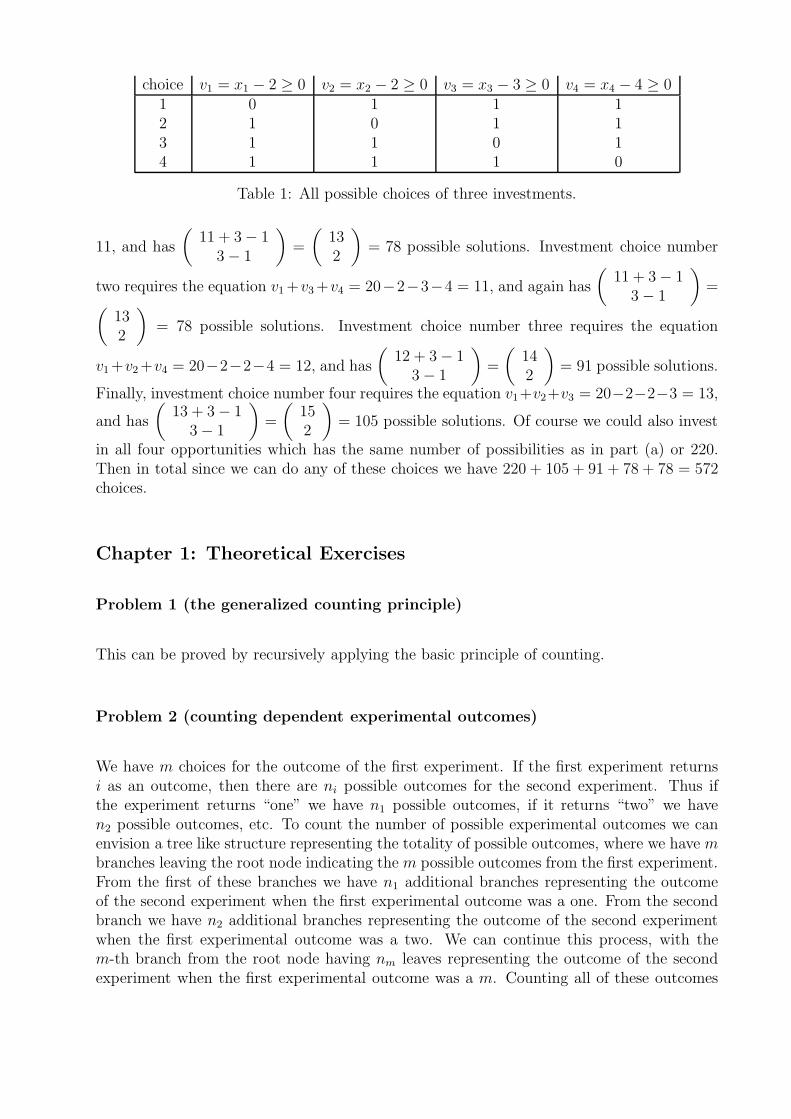
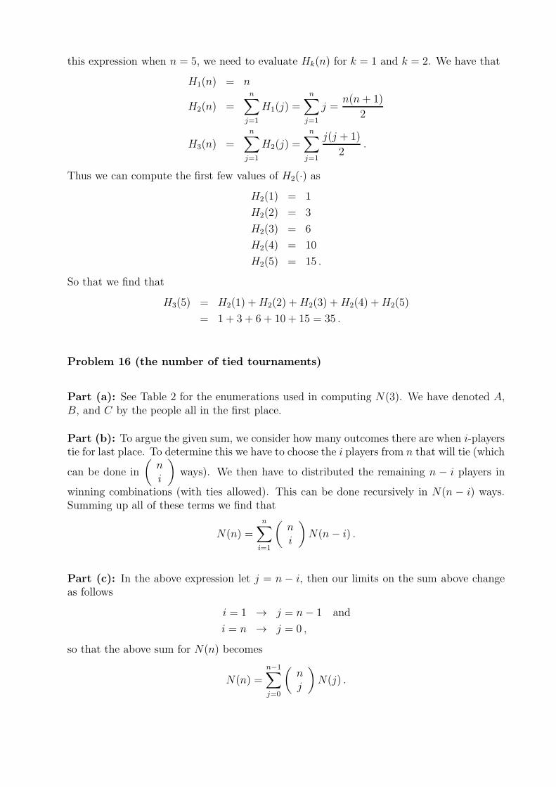
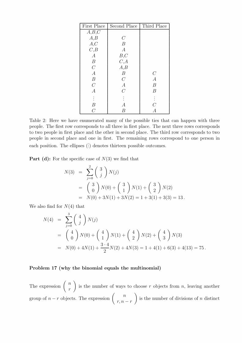
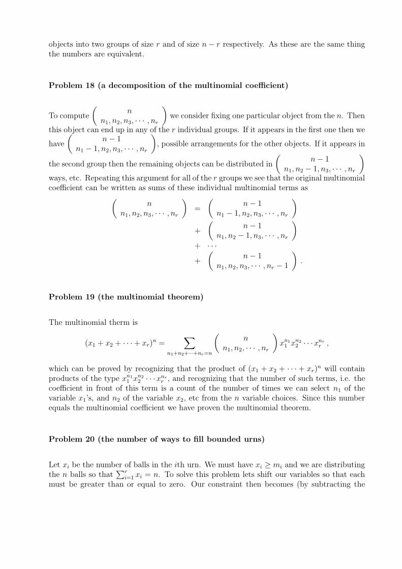
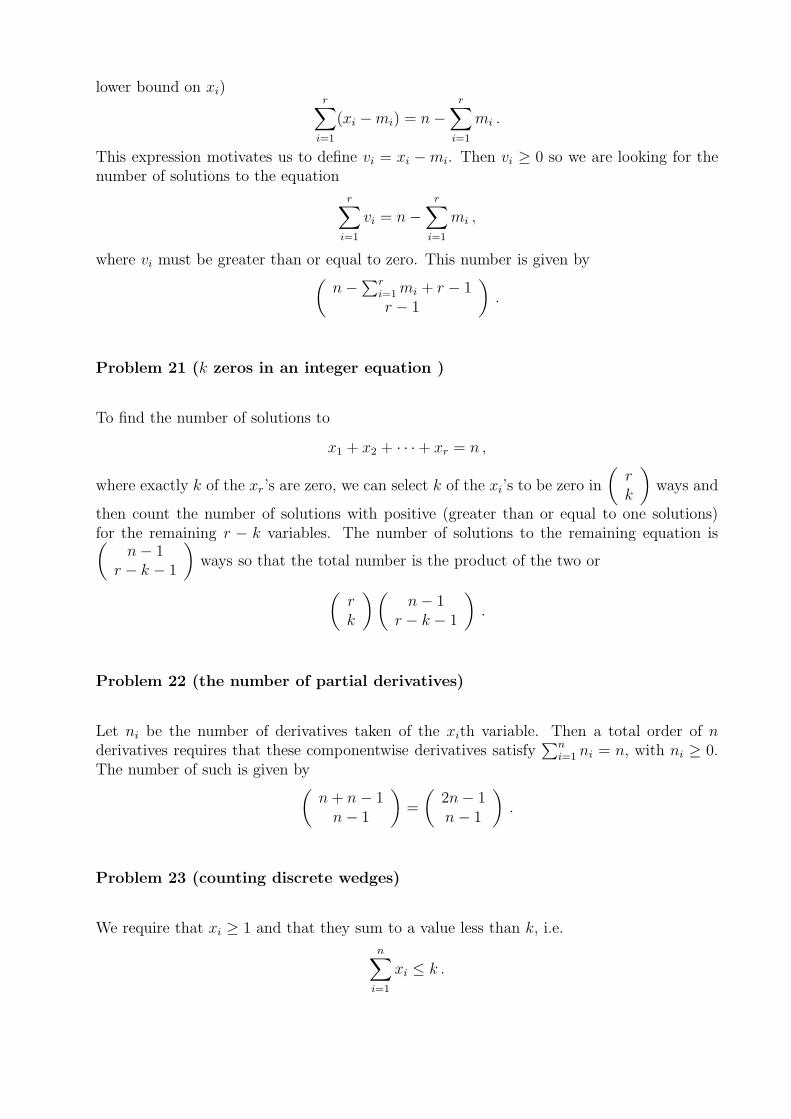
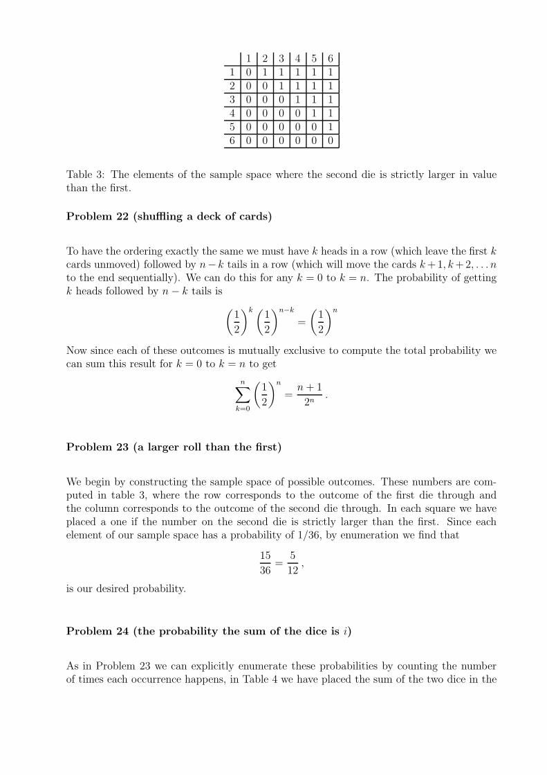
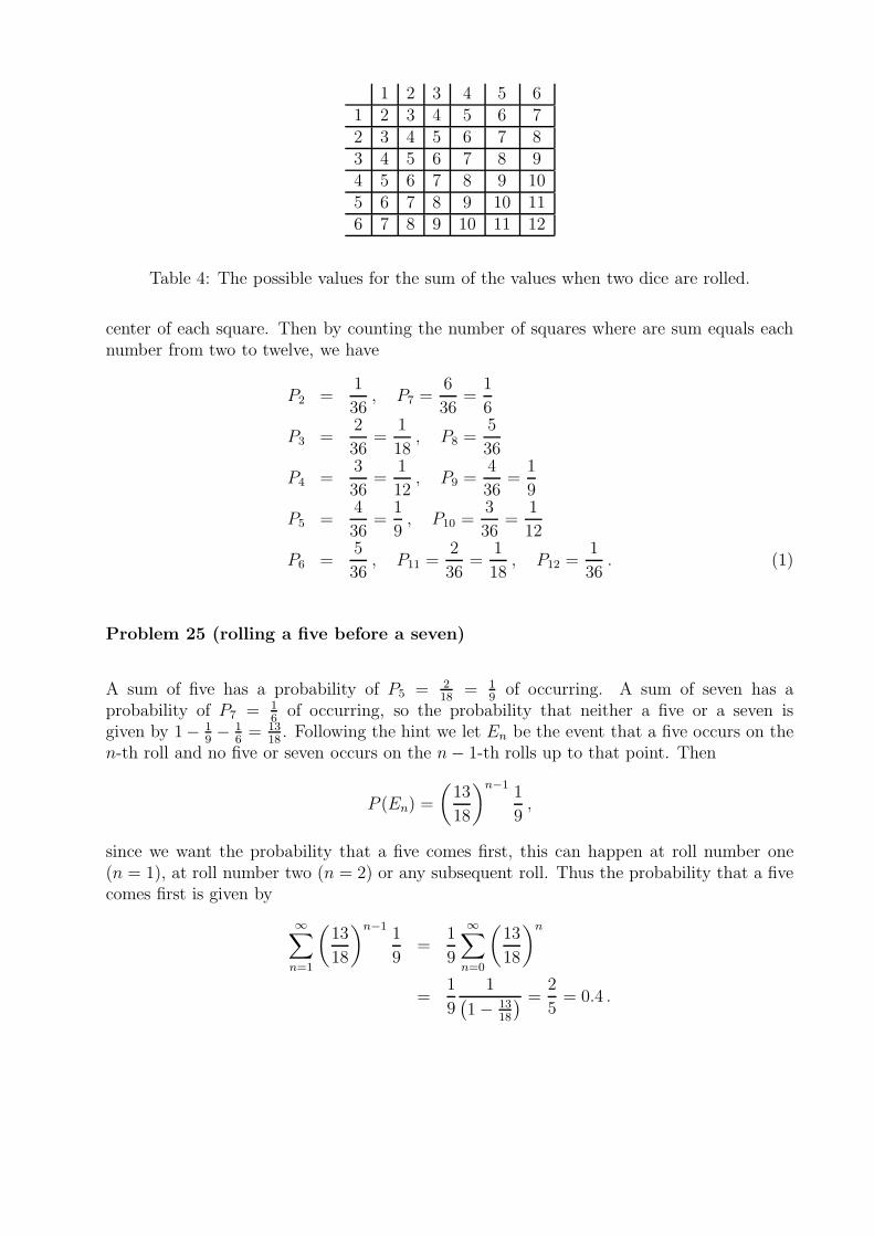

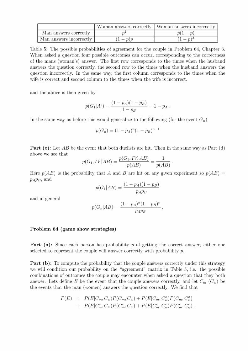
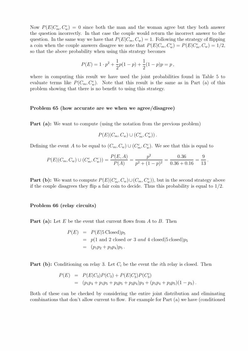
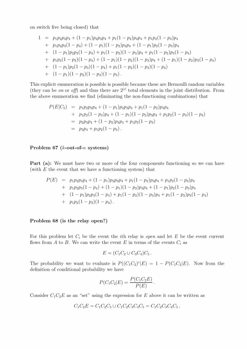
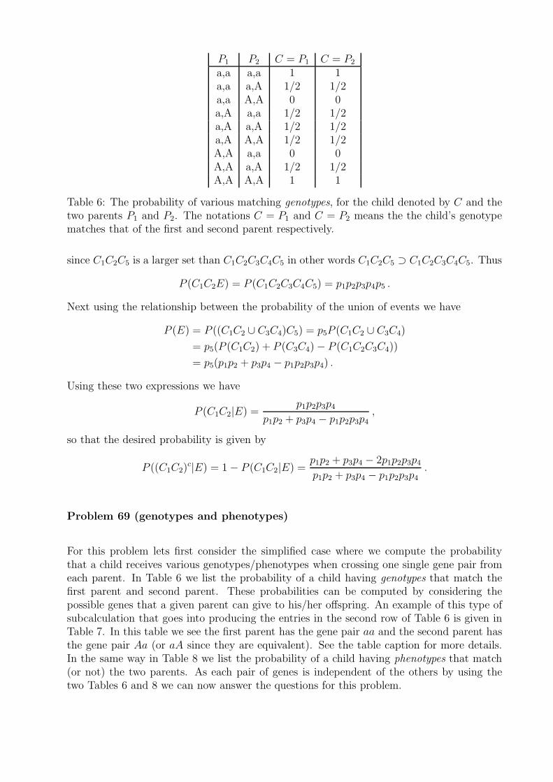
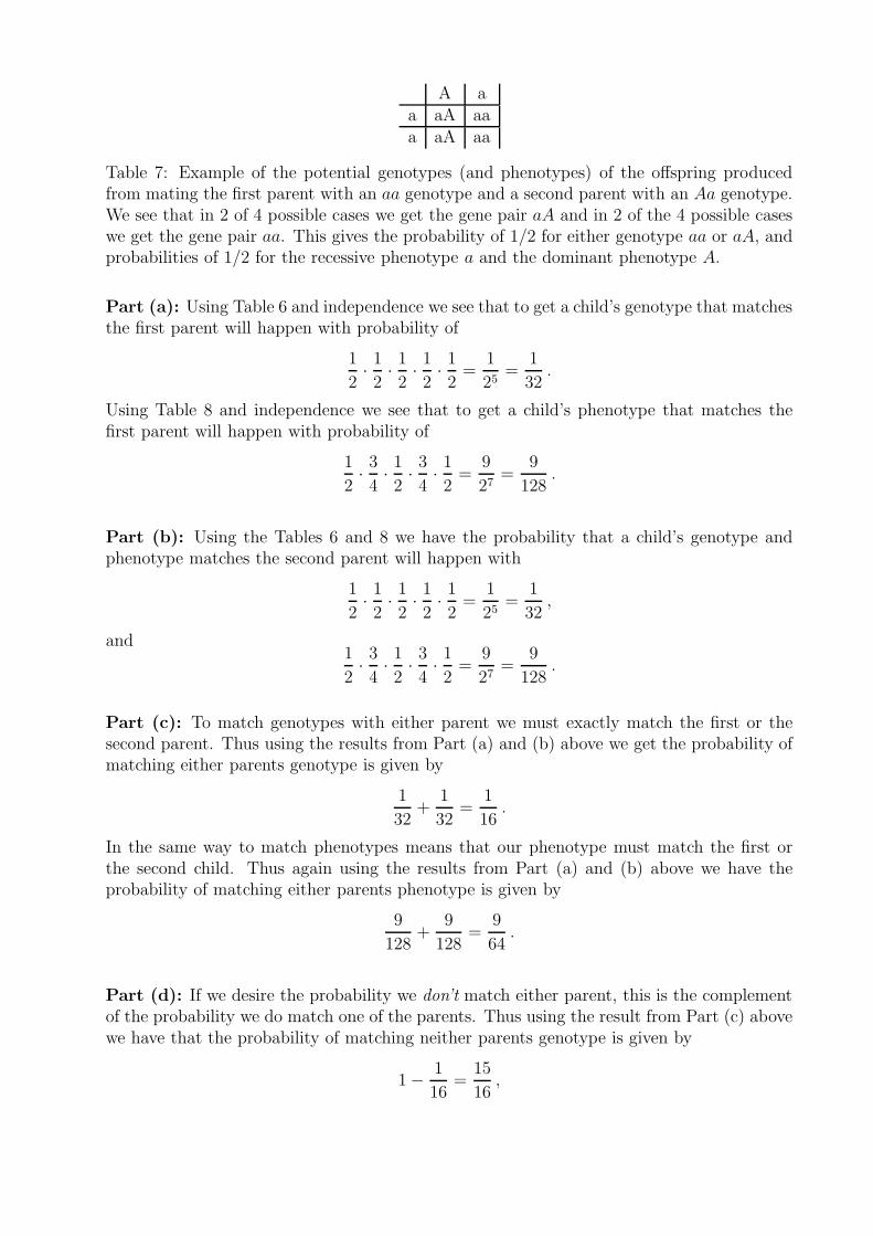
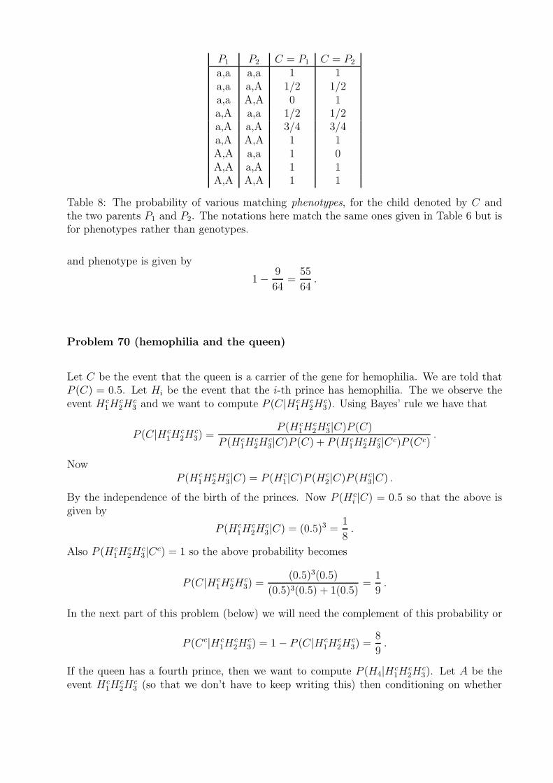
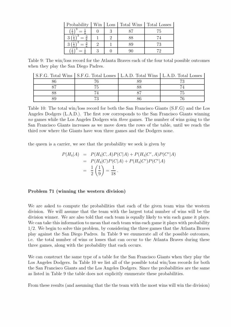
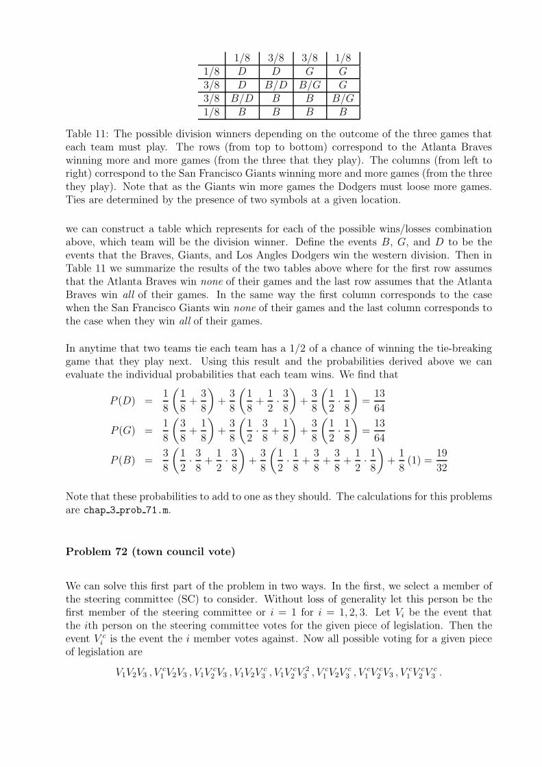
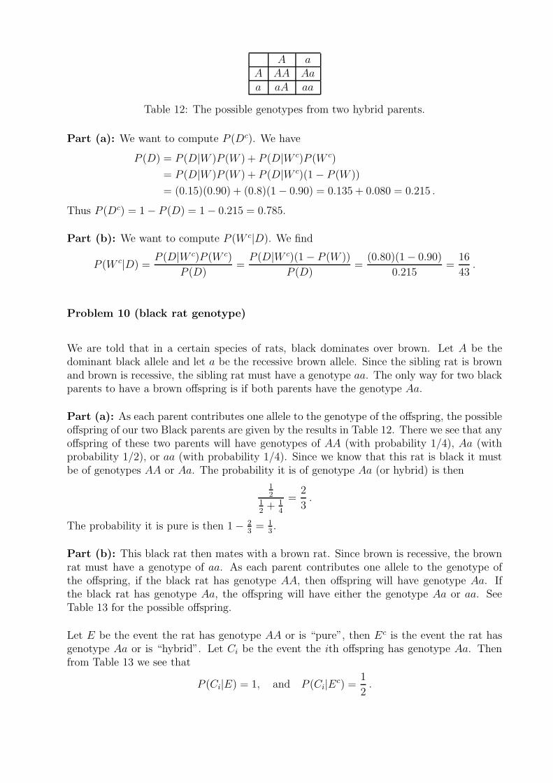
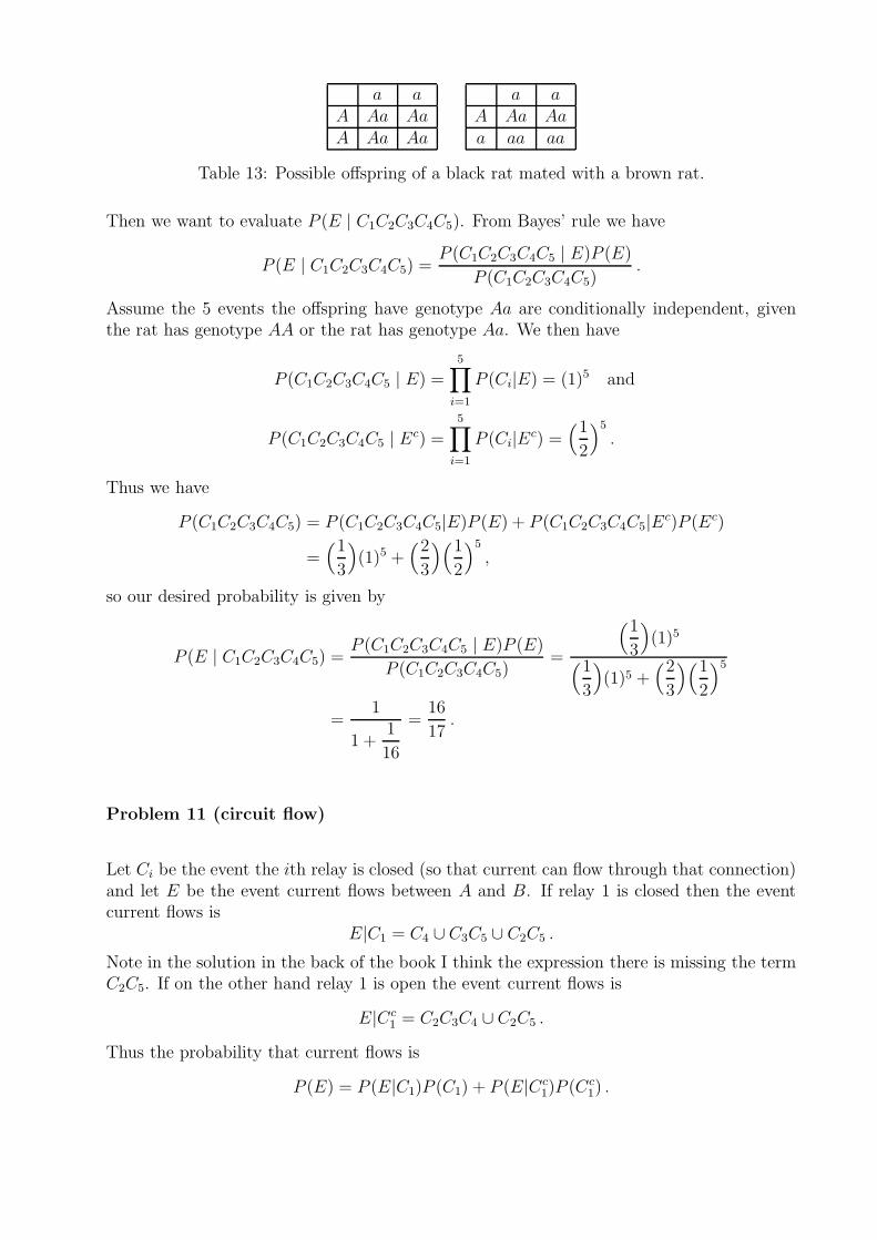
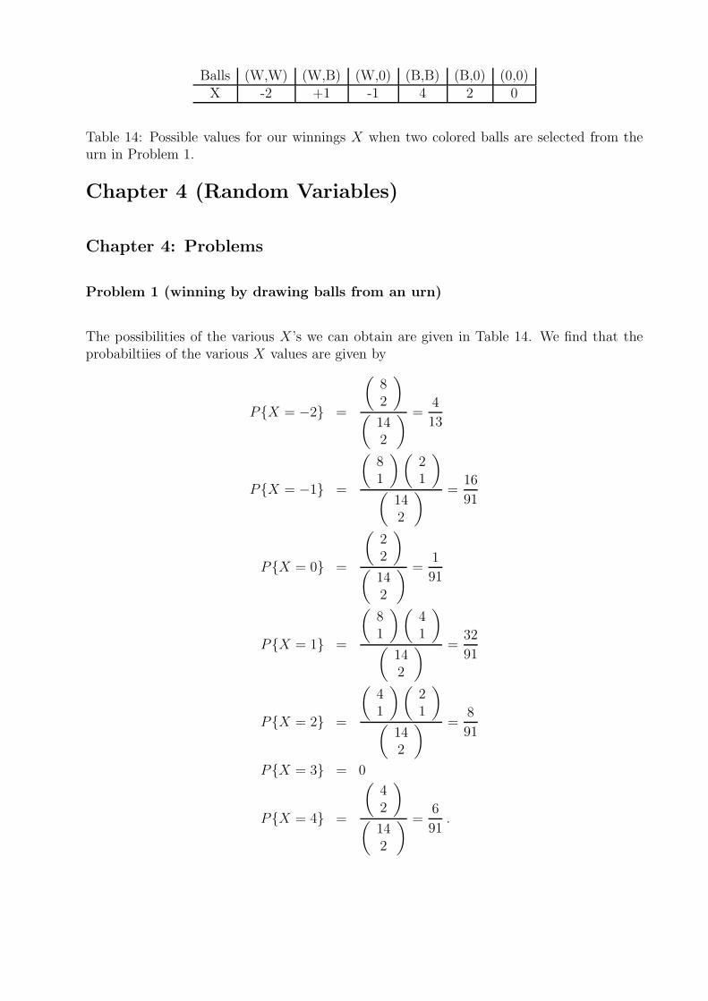
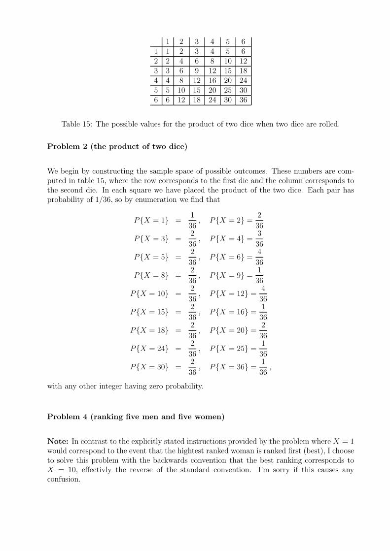
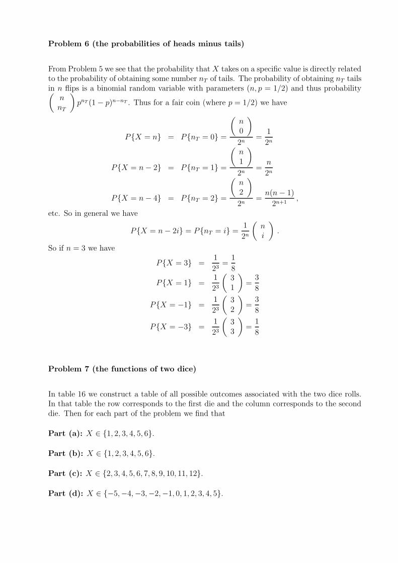
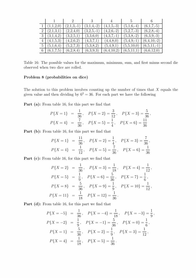
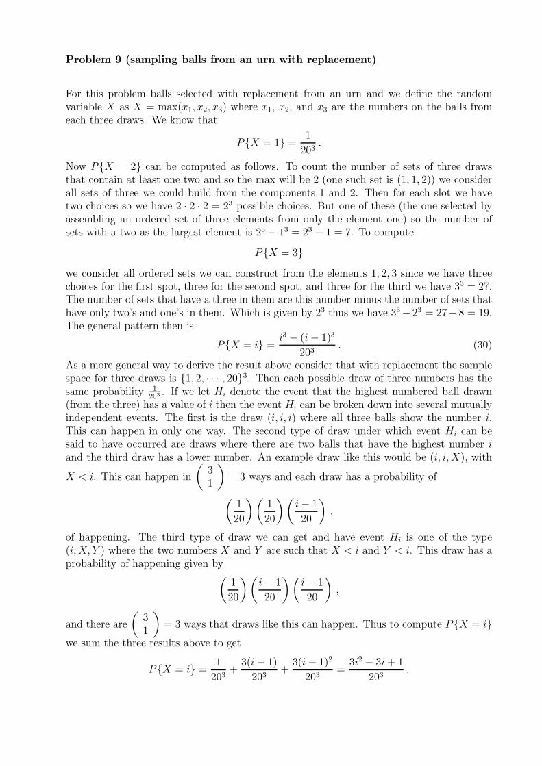
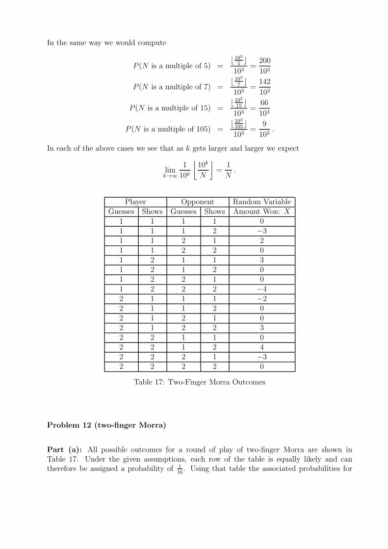
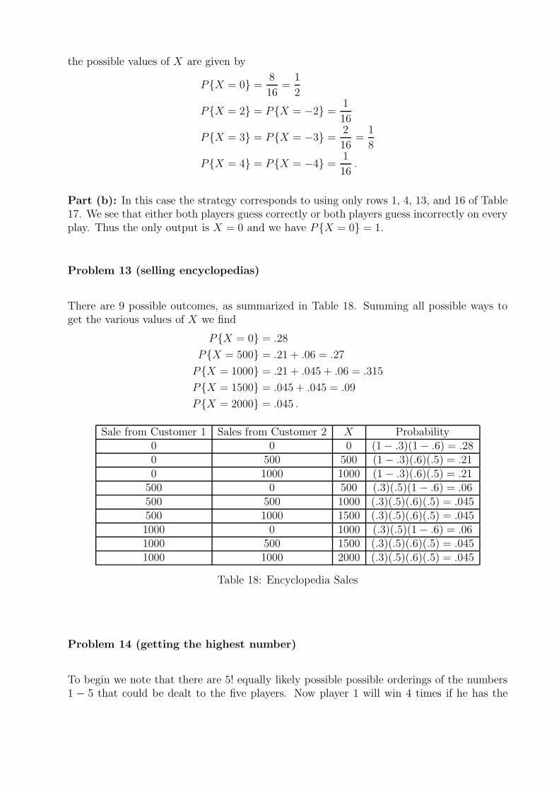
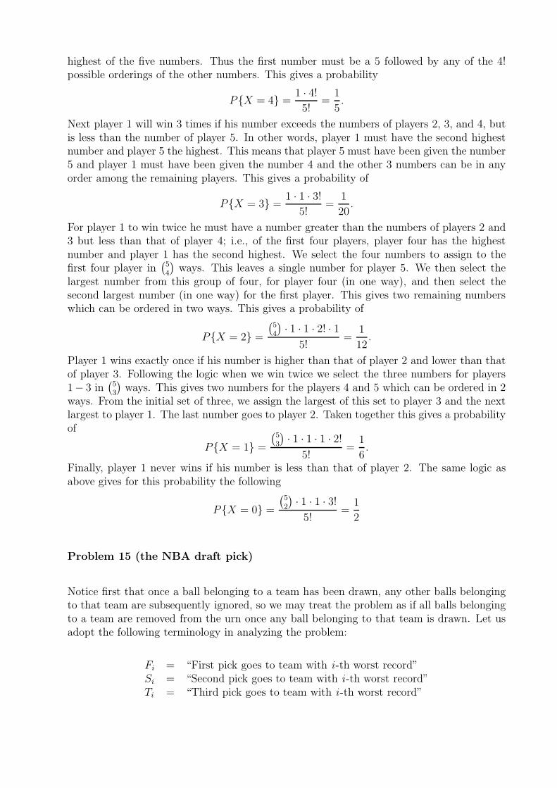
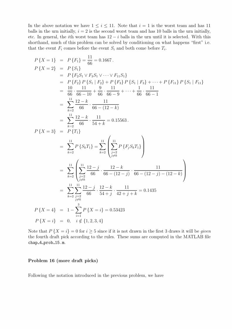
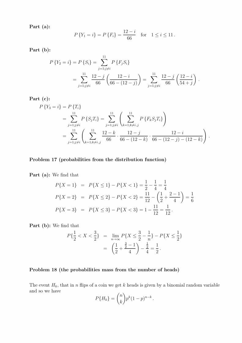
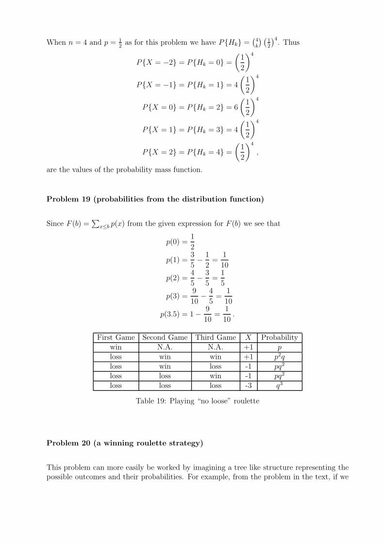
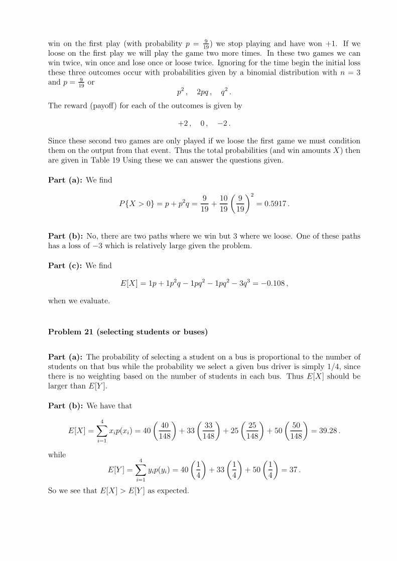
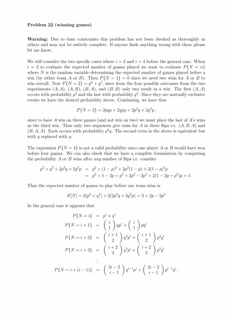
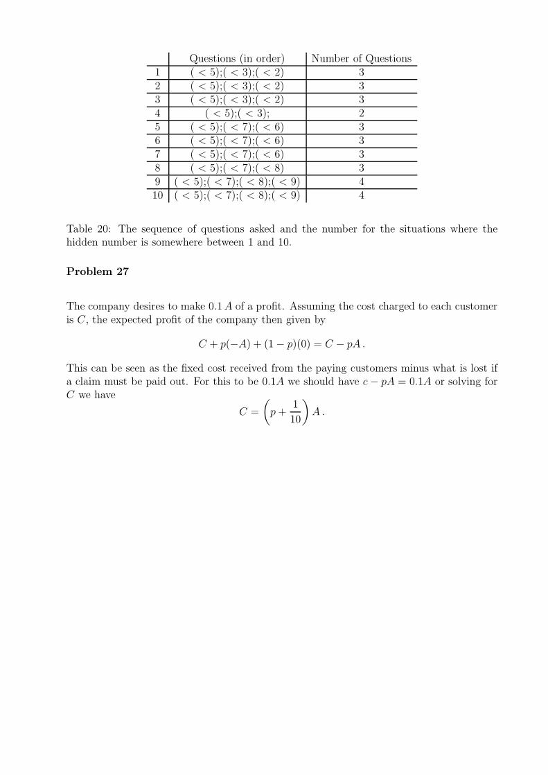
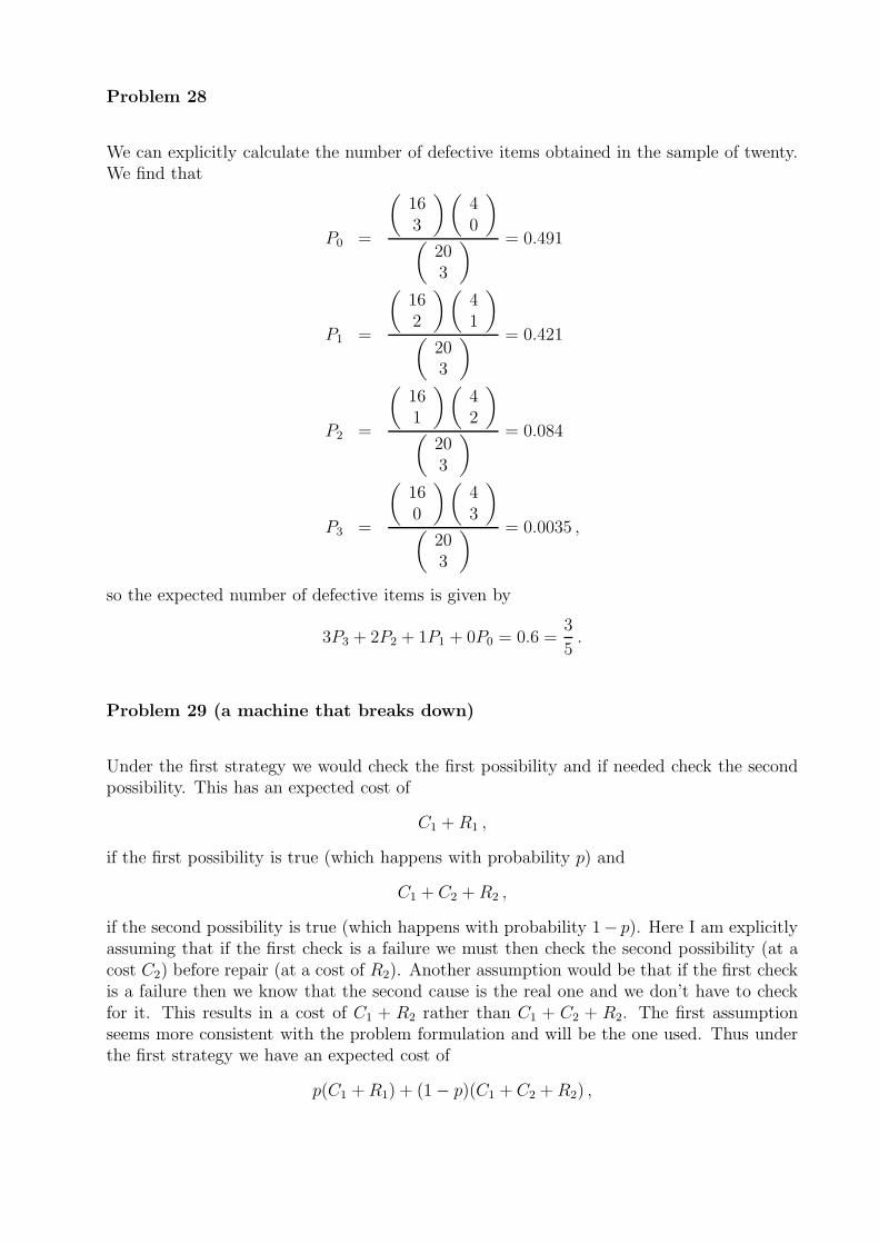
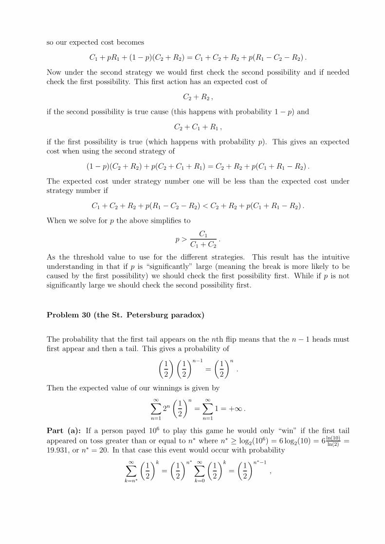
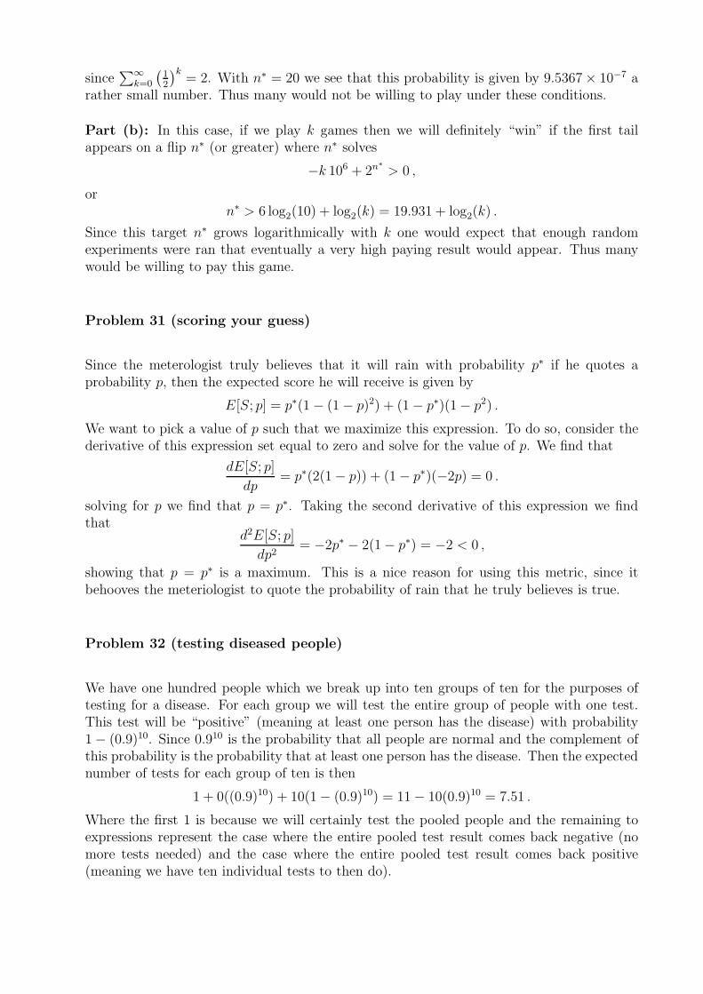
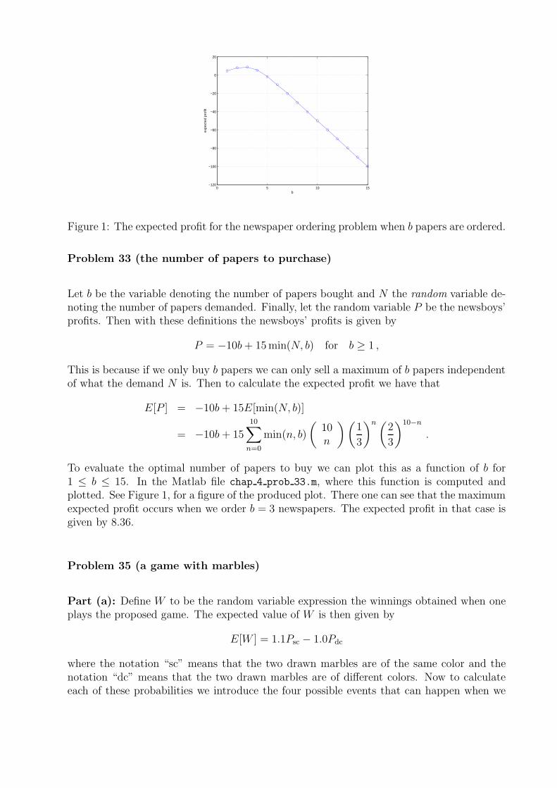

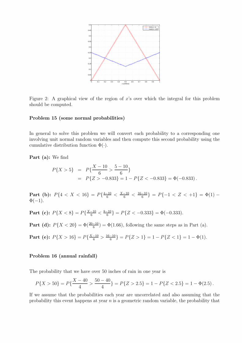
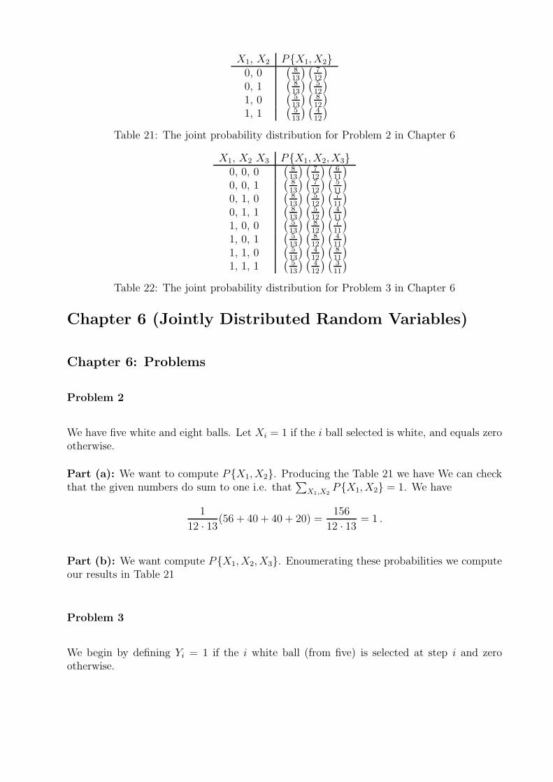
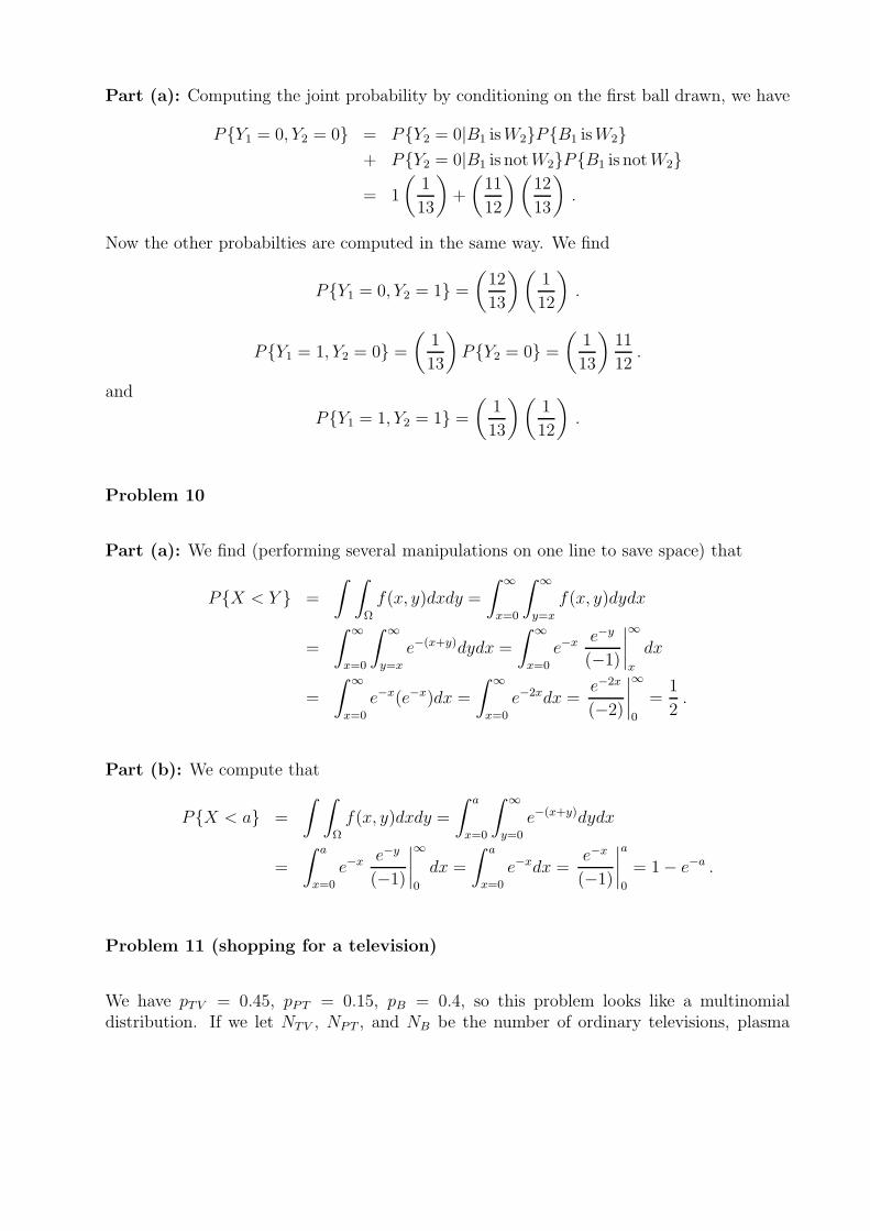
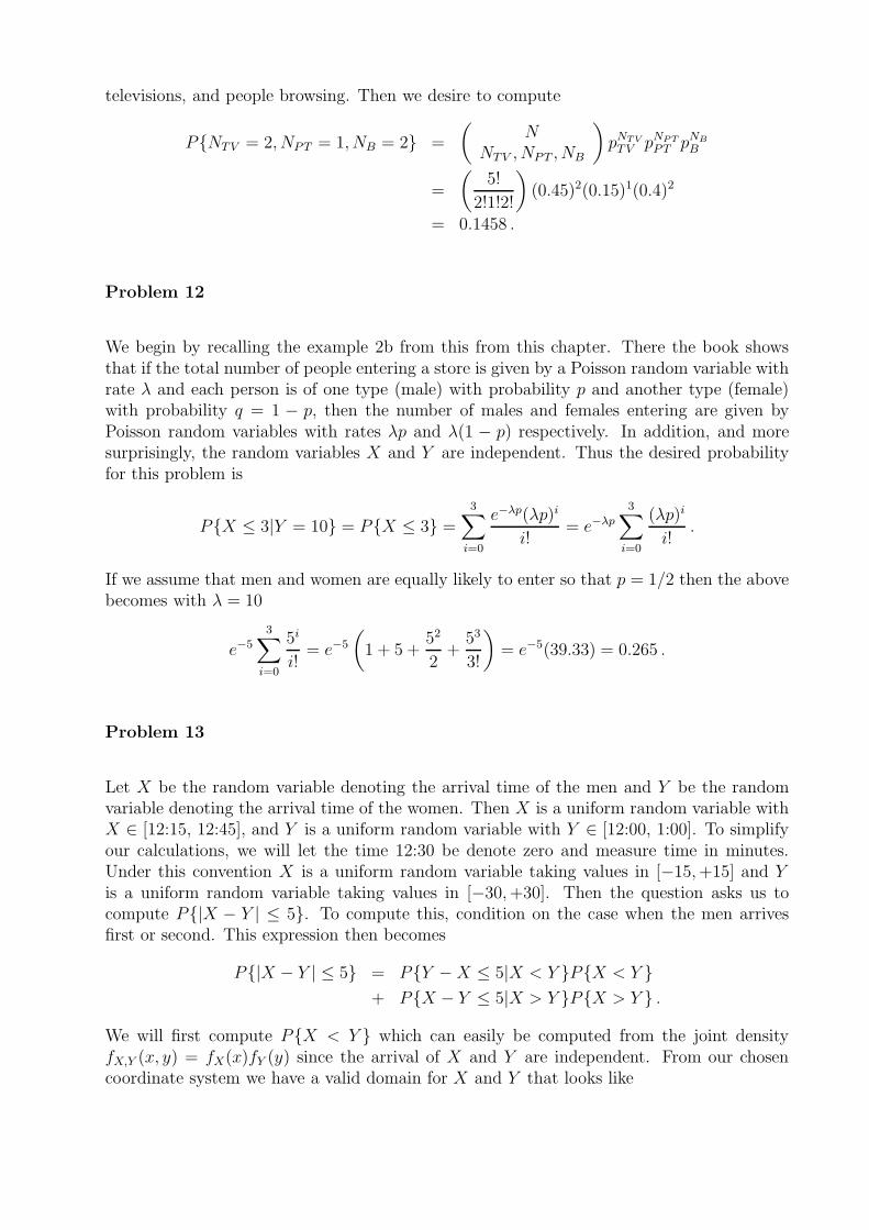
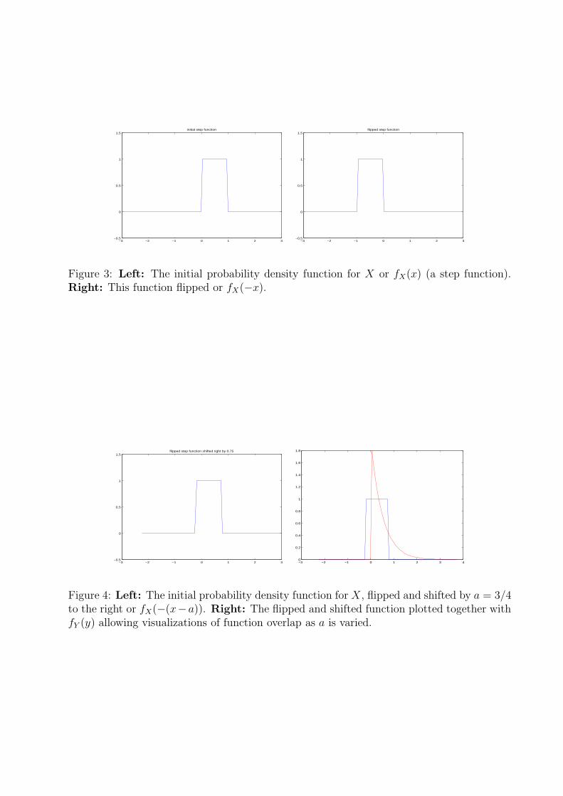
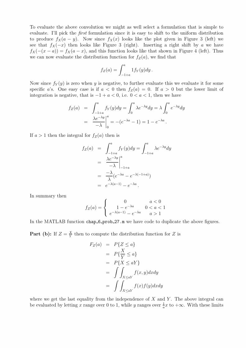
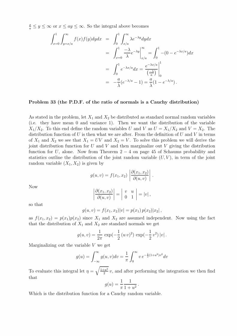
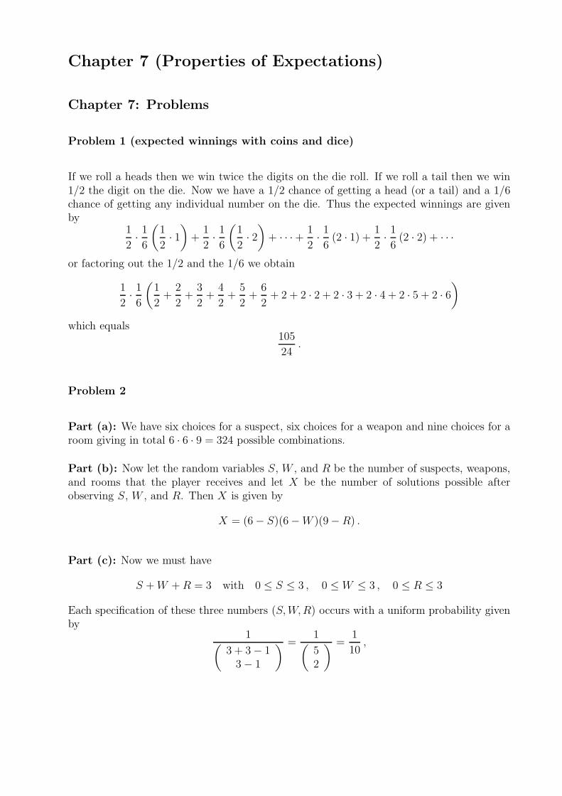
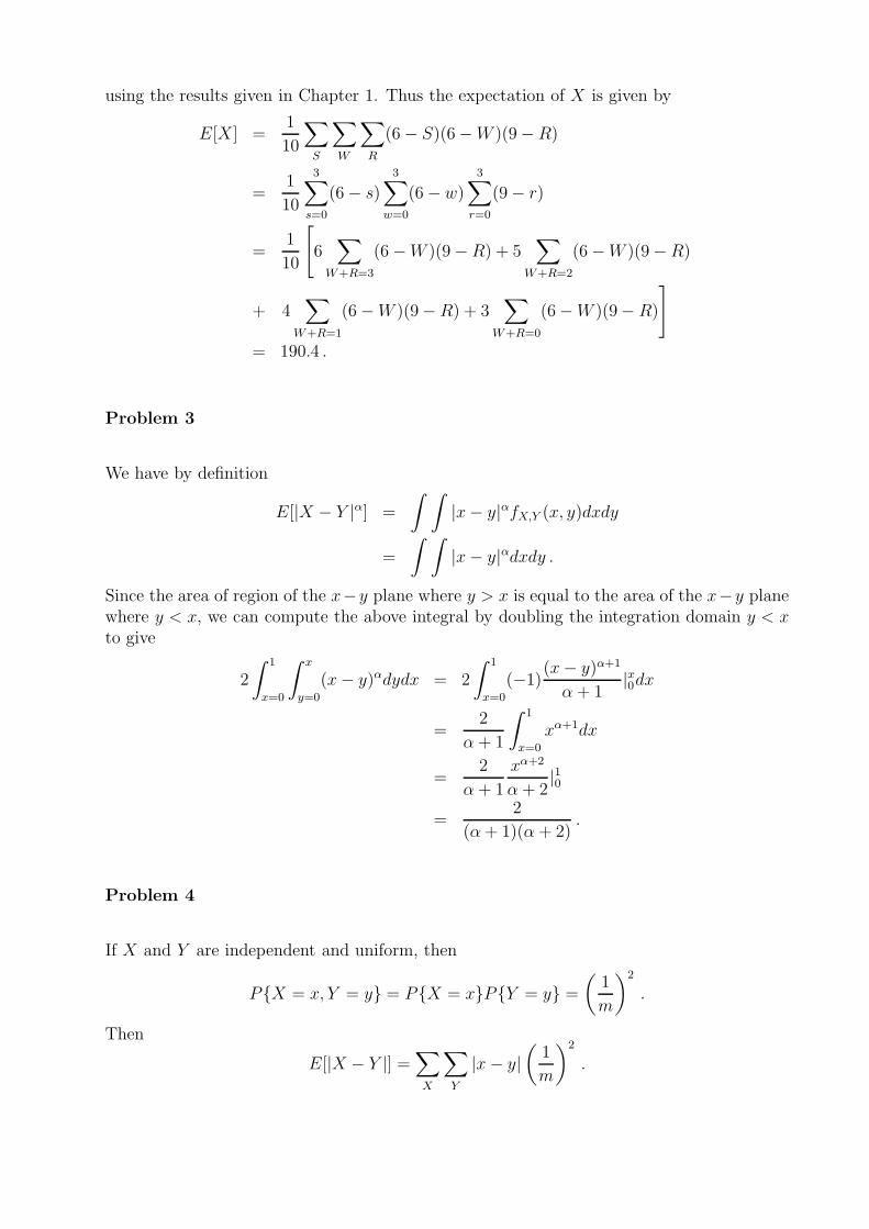
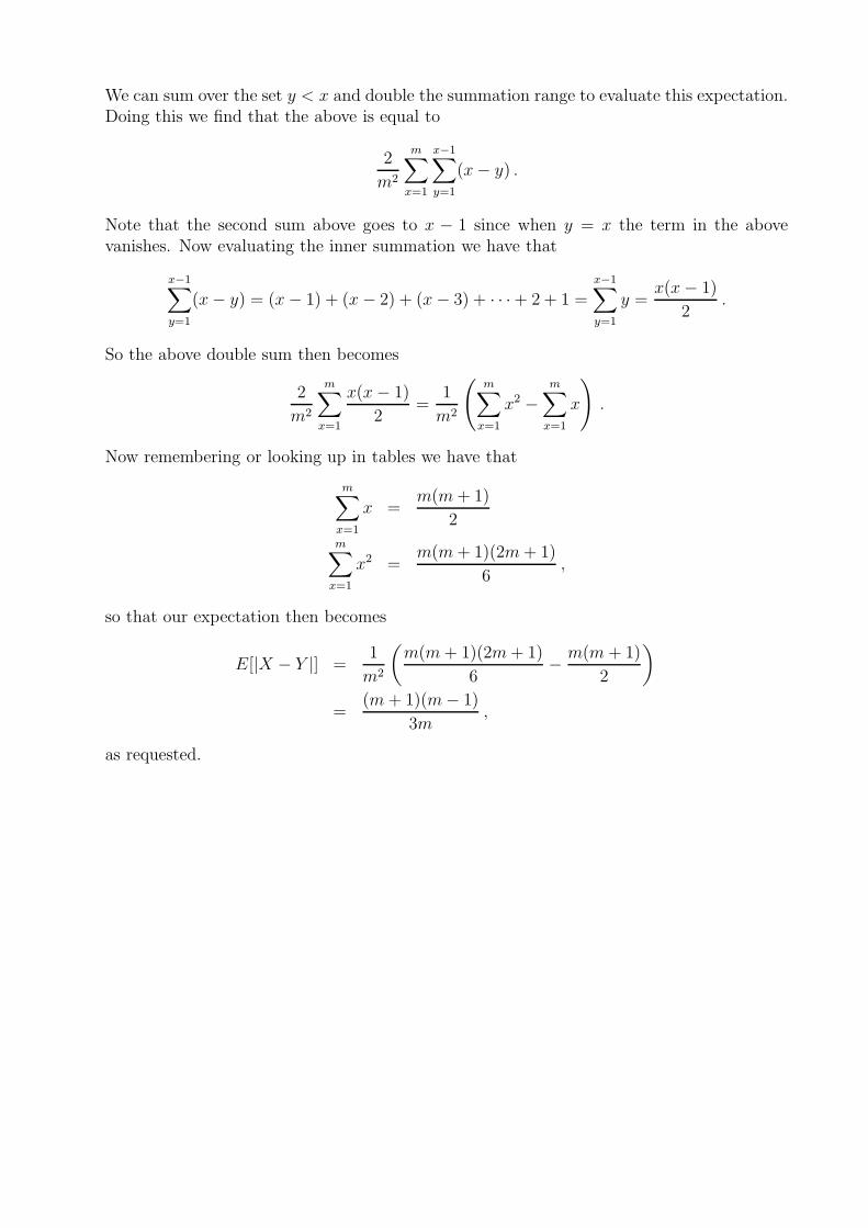
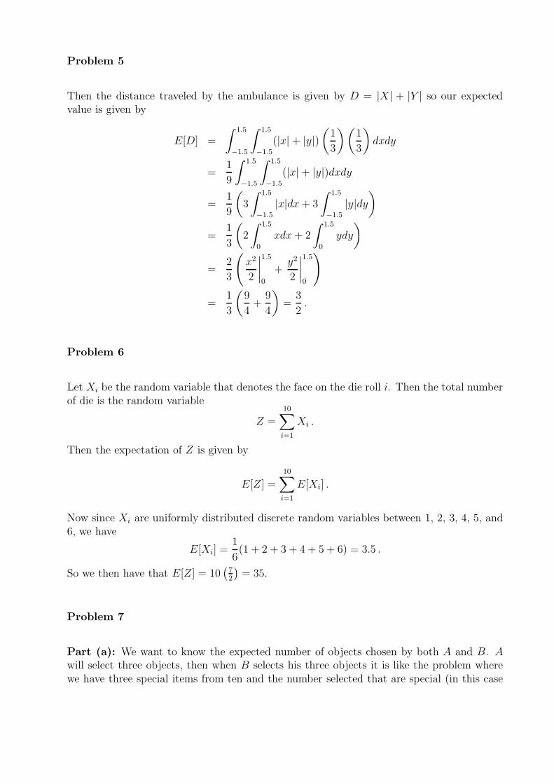
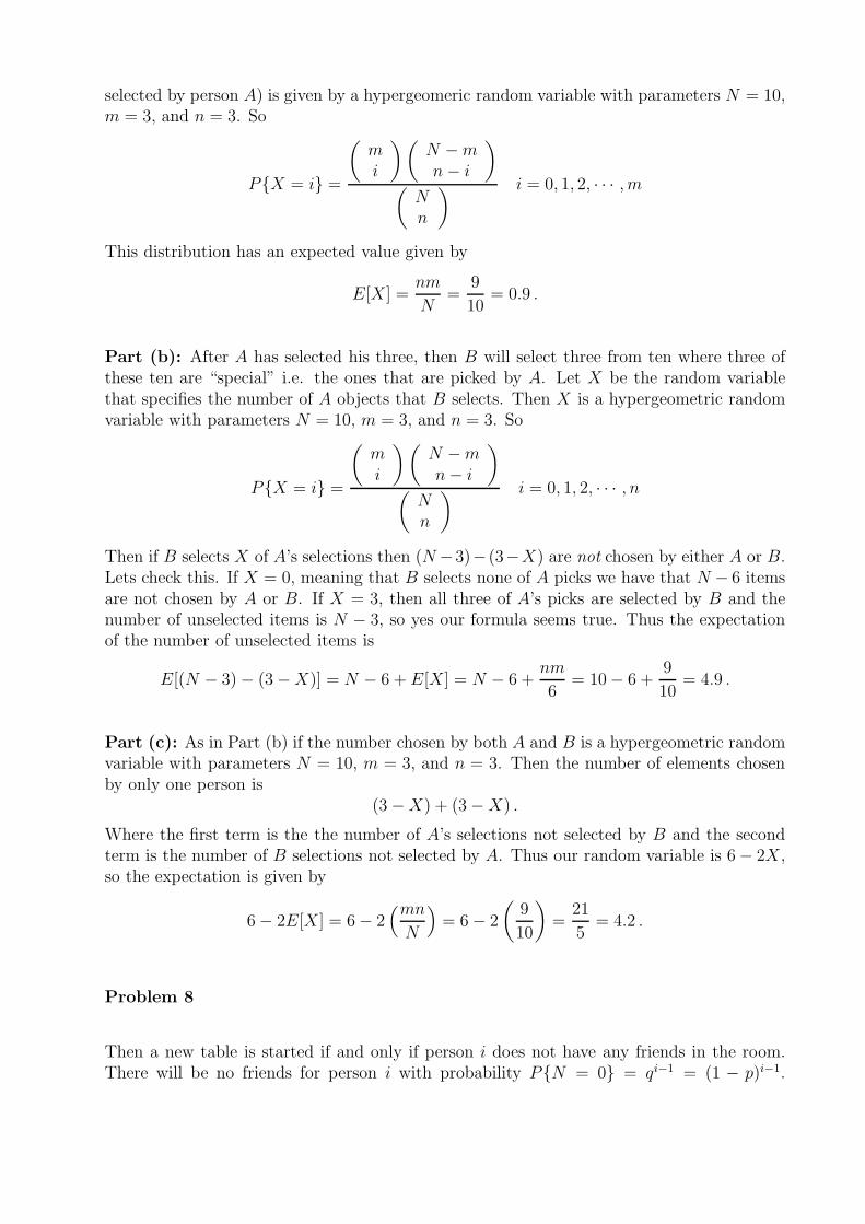
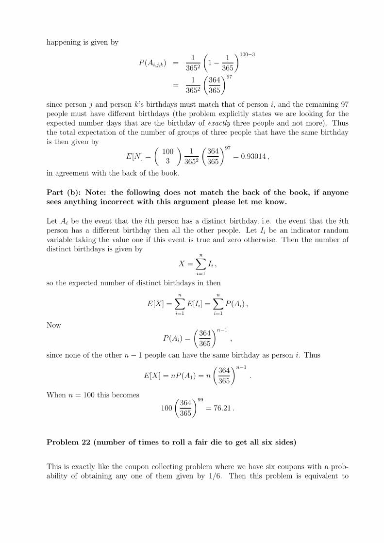
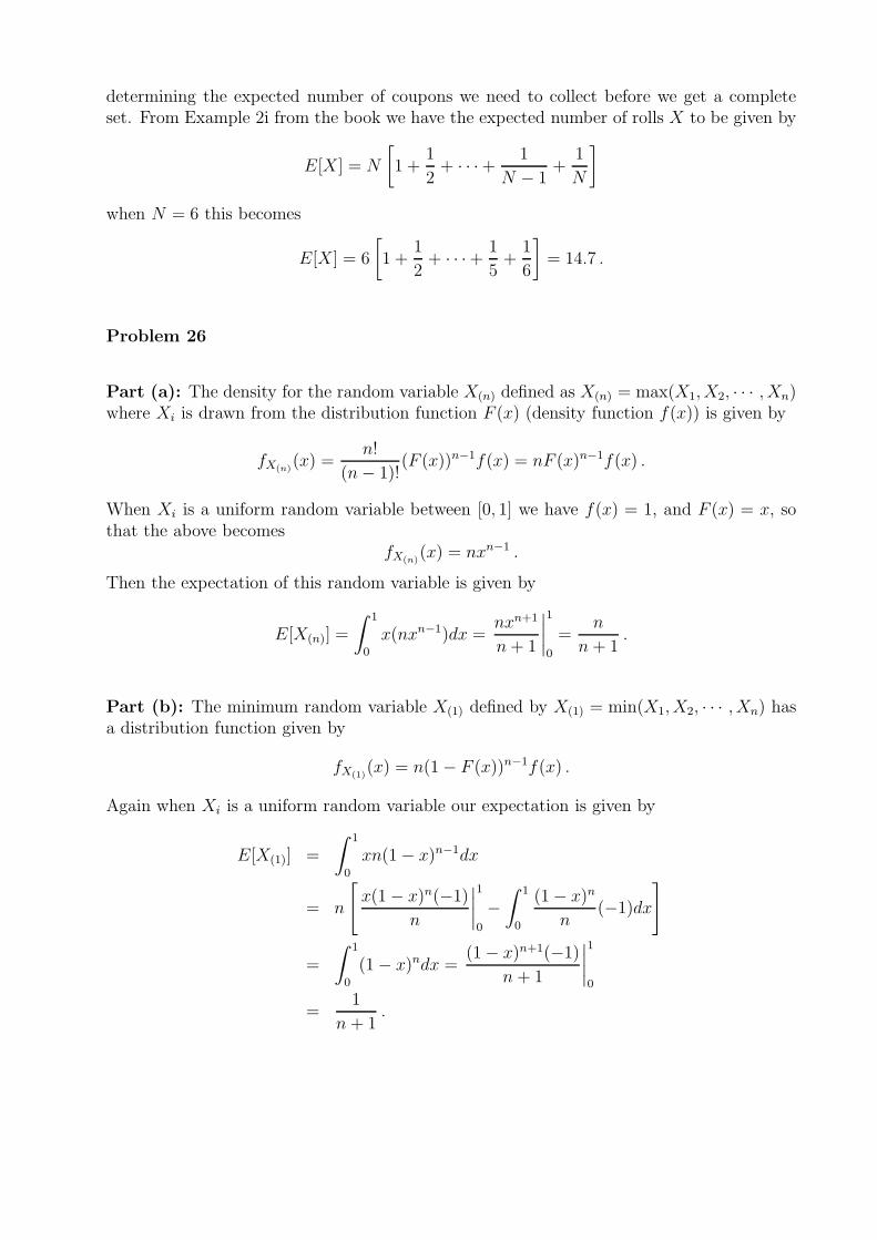
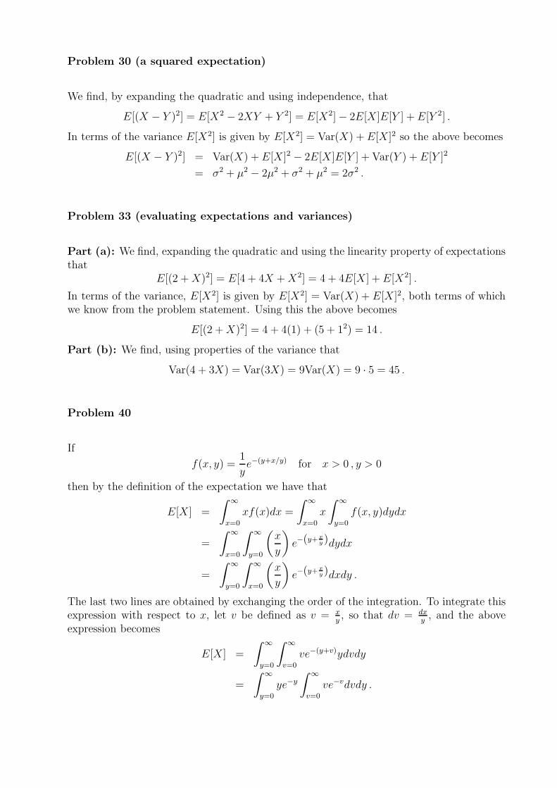
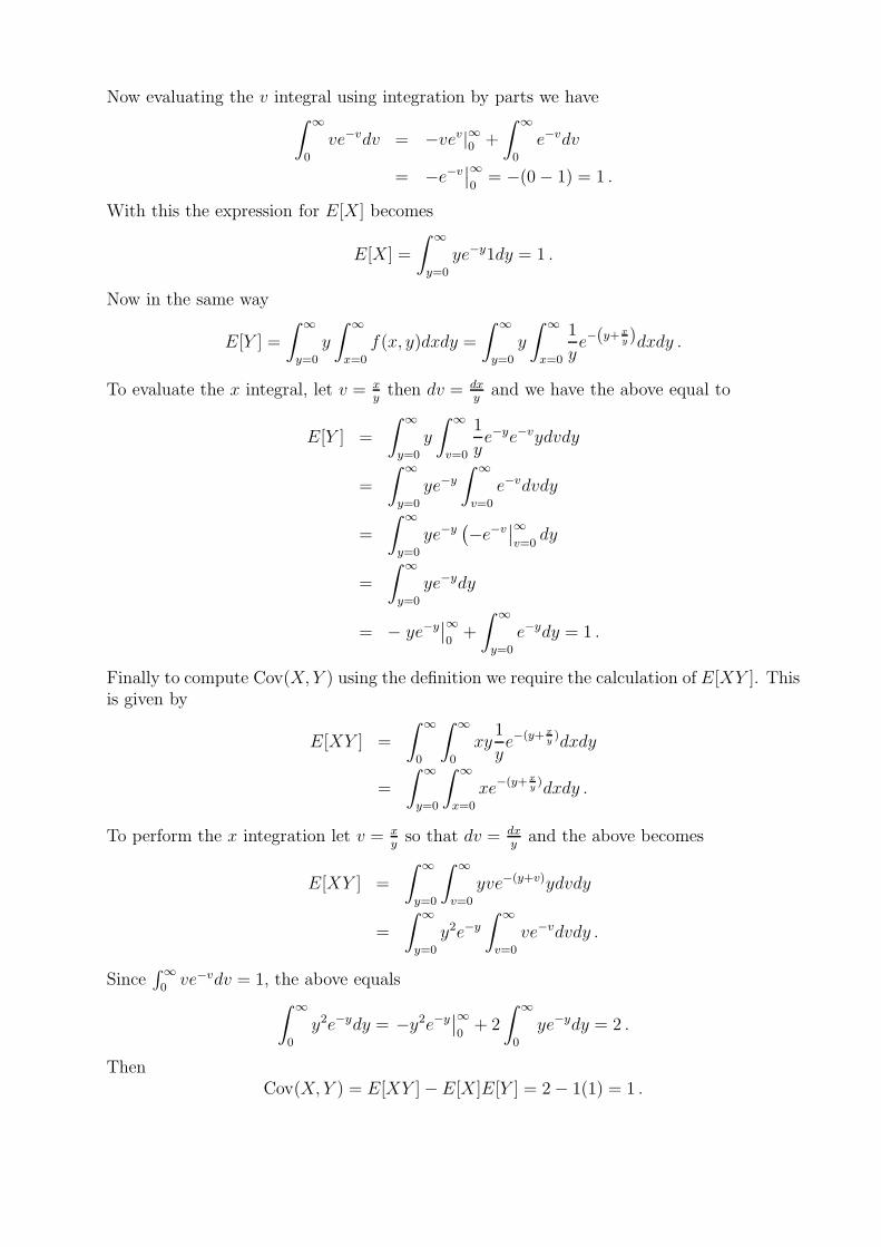
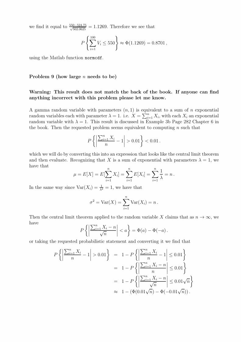
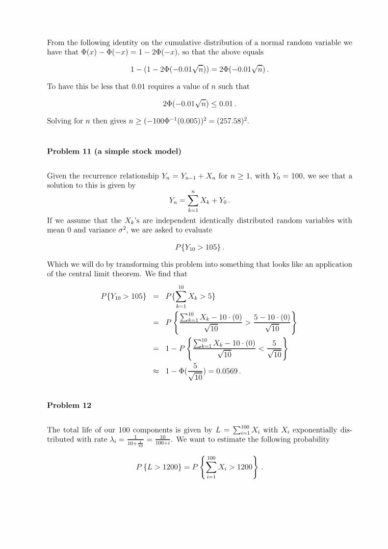
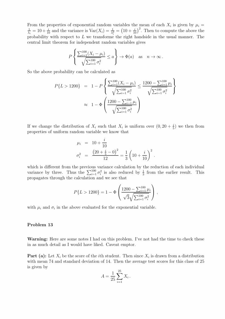
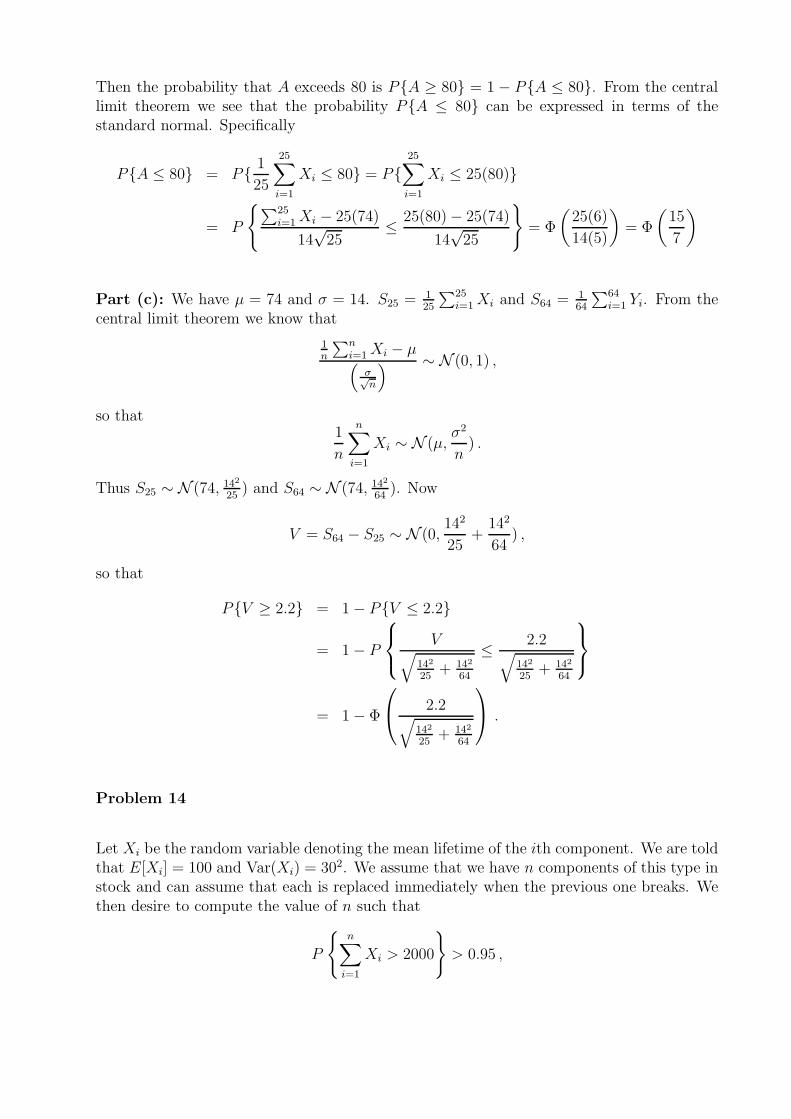


![Weatherwax Watkins Solutions[1]](https://static.documents.pub/doc/80x56/55cf9d5e550346d033ad543b/weatherwax-watkins-solutions1.jpg)


