400 Commonwealth Drive, Warrendale, PA 15096-0001 U.S.A. Tel: (724) 776-4841 Fax: (724) 776-5760 Web: www.sae.org SAE TECHNICAL PAPER SERIES 2004-01-2996 New Heat Transfer Correlation for an HCCI Engine Derived from Measurements of Instantaneous Surface Heat Flux Junseok Chang, Orgun Güralp, Zoran Filipi and Dennis Assanis University of Michigan Tang-Wei Kuo, Paul Najt and Rod Rask GM Research and Development Center Reprinted From: Homogeneous Charge Compression Ignition (SP-1896) Powertrain & Fluid Systems Conference & Exhibition Tampa, Florida USA October 25-28, 2004 Downloaded from SAE International by Ohio State University Center for Automotive Research, Wednesday, July 02, 2014
Downloaded from SAE International by Ohio State University Center for Automotive Research, Wednesday, July 02, 2014
All rights reserved. No part of this publication may be reproduced, stored in a retrieval system, ortransmitted, in any form or by any means, electronic, mechanical, photocopying, recording, or otherwise,without the prior written permission of SAE.
For permission and licensing requests contact:
SAE Permissions400 Commonwealth DriveWarrendale, PA 15096-0001-USAEmail: [email protected]: 724-772-4891Tel: 724-772-4028
For multiple print copies contact:
SAE Customer ServiceTel: 877-606-7323 (inside USA and Canada)Tel: 724-776-4970 (outside USA)Fax: 724-776-1615Email: [email protected]
Persons wishing to submit papers to be considered for presentation or publication by SAE should send themanuscript or a 300 word abstract of a proposed manuscript to: Secretary, Engineering Meetings Board, SAE.
Printed in USA
Downloaded from SAE International by Ohio State University Center for Automotive Research, Wednesday, July 02, 2014
1
2004-01-2996
New Heat Transfer Correlation for an HCCI Engine Derived from Measurements of Instantaneous Surface Heat Flux
Junseok Chang, Orgun Güralp, Zoran Filipi and Dennis Assanis University of Michigan
Tang-Wei Kuo, Paul Najt and Rod Rask GM Research and Development Center
An experimental study has been carried out to provide qualitative and quantitative insight into gas to wall heat transfer in a gasoline fueled Homogeneous Charge Compression Ignition (HCCI) engine. Fast response thermocouples are embedded in the piston top and cylinder head surface to measure instantaneous wall temperature and heat flux. Heat flux measurements obtained at multiple locations show small spatial variations, thus confirming relative uniformity of in-cylinder conditions in a HCCI engine operating with premixed charge. Consequently, the spatially-averaged heat flux represents well the global heat transfer from the gas to the combustion chamber walls in the premixed HCCI engine, as confirmed through the gross heat release analysis. Heat flux measurements were used for assessing several existing heat transfer correlations. One of the most popular models, the Woschni expression, was shown to be inadequate for the HCCI engine. The problem is traced back to the flame propagation term which is not appropriate for the HCCI combustion. Subsequently, a modified model is proposed which significantly improves the prediction of heat transfer in a gasoline HCCI engine and shows very good agreement over a range of conditions.
INTRODUCTION
Auto-ignition and combustion rates in a Homogeneous Charge Compression Ignition (HCCI) engine are very closely coupled to the heat transfer phenomena. Hence, a thorough understanding of the heat transfer process is critical for extending the load range and managing thermal transients. An improved heat transfer model, valid for a range of HCCI conditions, is an essential element in the development of predictive thermo-kinetic simulations.
The fuel, air and residual gas are generally expected to be well mixed in an HCCI engine and its combustion is often described as controlled auto-ignition. The combustion process starts at multiple locations and is governed by chemical kinetic rather than turbulent flame front propagation, as in Spark Ignition (SI) engines, or a stratified diffusion flame, as in conventional highly stratified Compression Ignition (CI) engines [1]. Hence, turbulence and mixing rates have a much smaller effect on HCCI combustion [2-5], while in-cylinder thermal conditions have a critical impact on HCCI ignition timing and burning rate. The thermal condition of the combustion chamber is closely tied to heat transfer from the hot gas to the walls. Thus, good understanding of the heat transfer process in the combustion chamber is prerequisite for developing HCCI engine control strategies and thermal management schemes.
A wealth of literature has been published over the years regarding the gas-to-wall heat transfer process in SI and CI engines and a number of correlations have been proposed for calculating the instantaneous heat transfer coefficient [6-15]. These studies have generally relied on dimensional analysis for turbulent flow that correlates the Nusselt, Reynolds, and Prandtl numbers. Using experiments in spherical vessels or engines and applying the assumption of quasi-steady conditions has led to empirical correlations for both SI and CI engine heat transfer. These correlations provide a heat transfer coefficient representing a spatially-averaged value for the cylinder. Hence, they are commonly referred to as global heat transfer models, e.g. Annand [8], Woschni [10] or Hohenberg [14]. In particular, the Woschni correlation has frequently been used for HCCI engine studies, even though the conditions in the engine vary significantly from those considered in the original work aimed at CI engines.
Downloaded from SAE International by Ohio State University Center for Automotive Research, Wednesday, July 02, 2014
2
Therefore, this paper is focused on experimentally investigating the heat transfer in an HCCI engine and using the newly acquired insight for developing a heat transfer correlation applicable to typical HCCI energy release. The dominant heat transfer mechanism in the HCCI engine is forced convection from the bulk gas to combustion chamber walls. The radiation effect is very small because of low-soot, low temperature combustion of the premixed lean mixture in a typical HCCI engine. While the “homogeneity” of the cylinder contents in the HCCI engine cylinder should not be interpreted as absolute, the conditions during combustion are expected to be relatively uniform. The spatial uniformity of the thermal conditions in the chamber is examined through heat flux measurements at multiple locations. Confirming this hypothesis would allow using averaged local heat flux measurements for evaluating a global heat transfer model for a well-mixed HCCI engine.
The validity of the approach can be checked by performing heat release analysis and confirming that adding heat loss to calculated net heat release satisfies energy balance. This is in great contrast to SI and CI engines, where it is difficult to get the area-averaged heat flux based on local measurements because of very high spatial variations [11, 27]. In the case of SI combustion, the flame front separates the chamber into a burned hot zone and a much cooler unburned zone. In the case of CI (diesel) combustion, the nature of burning is so heterogeneous that heat flux at any point indicates only conditions in the close proximity of the probe.
The engine used in this study is a single cylinder engine operated with a premixed charge of air and gasoline. The engine operates with re-breathing, i.e. the exhaust valve is opened one more time during the intake stroke to allow induction of hot residual and to help promote auto-ignition. The coaxial type fast-response thermocouples are installed flush with the surface of the piston and the cylinder head for measuring instantaneous temperature as a function of crank-angle. This type of sensor is selected due to its demonstrated favorable dynamic behavior when applied to heat flux measurements during the compression and firing conditions [16, 22] in a metal engine.
The paper is organized as follows. The experimental methodology is described in the next section. Then local heat flux measurements are used to assess spatial uniformity. Subsequently, the concept of spatially- averaged heat flux is introduced, verified through heat release analysis, and used for evaluation of classic heat transfer models. The analysis of deficiencies associated with the Woschni classic model when applied to an HCCI engine leads to the proposed modification of the model in a two-stage process. Finally, the behavior of the new convective heat transfer correlation is verified over the range of operating conditions, followed by conclusions.
EXPERIMENTAL METHODOLOGY
HCCI ENGINE SET-UP
A modified Ricardo Hydra single cylinder engine is used for engine dynamometer tests. A GM prototype, pent- roof shape cylinder head is designed specially for this experiment, but basic features correspond to a typical modern 4-valve cylinder head. Table 1 indicates engine specifications.
Table1. Engine Specifications Engine Type 4 valves, single cylinderBore / Stroke 86.0 / 94.6mmDisplacement 0.5495 literConnecting Rod Length 152.2 mmCompression Ratio 12.5IVO / IVC 346o / 592o *Main EVO / EVC 130o / 368o * 2nd EVO / EVC 394o / 531o *Fuel Type Gasoline (H/C=1.898)* 0o crank angle is assigned as TDC Combustion.
Figure 1: Schematic of HCCI engine setup
An exhaust re-breathing strategy is applied to provide the necessary residual fraction for HCCI combustion control. This involves the exhaust valves opening for a second time during the intake stroke via an additional lobe on the exhaust cam. During this period, hot exhaust residual gas is drawn back into the cylinder to subsequently help with ignition during HCCI operation. The residual affects auto-ignition and combustion through a thermal and chemical effect. The exhaust back pressure is maintained at the level of ambient pressure by controlling the gate valve shown in Figure 1. One of the intake ports has a tangential shape and is
Downloaded from SAE International by Ohio State University Center for Automotive Research, Wednesday, July 02, 2014
3
intended to produce organized swirling motion, while the other contains a Swirl Control Valve (SCV)’ installed ~180mm upstream from the valve seat, see Figure 1. The SCV was originally devised to control the swirl/tumble intensity in the stratified direct injection SI version of the engine. However, the addition of the second lobe on the exhaust cam and use of the exhaust re-breathing strategy makes the flow pattern in the tested HCCI engine much less organized and reduces the impact of the SCV. Exhaust gas is sampled at the exhaust plenum for emissions measurement with gaseous analyzers measuring concentrations of HC, NOx, CO, CO2 and O2, thus allowing calculation of engine-out air/fuel ratio and combustion efficiency. A Kistler 6125A piezo-electric pressure transducer measures the pressure trace in the cylinder with 0.5o crank-angle resolution. A flame trap is installed in front of the transducer tip to avoid thermal shock, and 200 consecutive cycles are recorded at any given condition. Pressure signal filtering is performed based on a Savitzky-Golay filtering scheme [34]. To prevent phase shift after filtering, the filtered sequence is then reversed and run back through the filter. Top dead center is determined by considering the thermodynamic loss angle via the net heat release method suggested by Sta [35]. Absolute cylinder pressure referencing, or ‘pressure pegging’, is performed based on intake manifold absolute pressure [36]. The high-pressure fuel delivery system is based on a bladder-type accumulator. A bladder containing fuel is in a vessel pressurized by nitrogen. Regulating the pressure of N2 allows control of the fuel injection pressure. The fuel delivery line is split so that fuel can be introduced in an injector in the cylinder head for direct injection, or the injector in the vaporizer for fully premixed operation. Both injectors are identical DI-type designs. In this paper, all tests were performed with fully premixed charge in order to ensure homogeneous in-cylinder conditions. The fuel vaporizer consists of aluminum chamber surrounded by an electric band heater to maintain the inner surface temperature at ~220oC, measured by a thermocouple mounted 5 mm below the surface of the chamber. A reasonable air flow through the chamber is enabled by positioning the vaporizer air intake above the main throttle valve, thus ensuring the required pressure drop. A combination of carefully selected chamber temperature and pressure drop between air intake and charge outlet provides enough flow to prevent condensation in cold spots, and yet keeps the mixture well outside of the flammable limit. Vaporized fuel and air are then routed to the intake runner upstream of the plenum to ensure complete mixing.
INSTANTANEOUS SURFACE TEMPERATURE AND HEAT FLUX MEASUREMENT
A variety of surface thermocouple (TC) designs has been developed since Eichelberg’s first attempt to
measure instantaneous surface temperature in the combustion chamber in 1939 [6]. A surface junction on modern probes is formed by very thin metallic layers vacuum-deposited or chemically plated to obtain fast response time. Fast response thermocouples can be categorized in the following main groups: the coaxial [16, 18], the pair wire [16], and the thin film type. The former two are more widely used for measurements on metal surfaces, while the thin film design has been developed specifically for measurements on the surface of ceramic coatings and inlays [19, 20] with the intention of minimizing the disturbance in the temperature field due to the insertion of the probe. A coaxial type probe is selected for this study due to its demonstrated favorable dynamic behavior when applied to heat flux measurements during the compression and firing conditions [16, 22] in a metal engine. The schematic of the probe design is given in Figure 2. It consists of a thin wire of one TC material (Constantan) coated with a ceramic insulation of high dielectric strength, swaged securely in a tube of a second TC material (Iron). A vacuum-deposited metallic plate forms a metallurgical bond with the two TC elements, thus forming the TC junction with 1~2 micron thickness over the sensing end of the probe. The probes are custom manufactured by Medtherm Corporation [42] and their response time is on the order of a micro-second. The sensing area is mounted flush with the combustion chamber surface.
Figure 2: Schematics of Heat Flux Probe [42]
The main contribution to the total heat flux during firing conditions is the transient component of heat flux, and hence the accuracy of the surface thermocouple is critical. As long as the size of the hot junction is small enough, in this case its diameter is only 1.52 mm, the temperature between the ends of the center wire and the outer tube may be neglected [24]. The penetration of the thermal pulse into the surface is small in comparison with the relevant surrounding dimensions (αt/L2<<1) and a one-dimensional transient heat flux analysis can be used [21, 22, 23, 24]. Theoretical analysis based on finite element method [22], and experiments in the dynamic test rig [16] indicate high-accuracy of instantaneous temperature measurements (~98%), good ability of the probe to capture instantaneous rise of heat flux, but also the potential for overpredicting the peak heat flux due to dynamic phenomena within the probe i.e.
Downloaded from SAE International by Ohio State University Center for Automotive Research, Wednesday, July 02, 2014
4
the inability of the heat sink surrounding the center wire to cool it fast enough to control the transient response. The error is minimized if correct thermal properties of the probe body are used, in this case conductivity is k=57.11 (W/m-K) and diffusivity α=16.26*E-6 (m2/s). Another potential source of error is the presence of combustion deposits on the surface of the probe, and this can offset the tendency to overpredict the peak heat flux in a practical engine application. In addition, the peak heat flux is not the main quantitative indicator of the heat transfer phenomena, rather it is the combination of overall features of the crank-angle resolved heat flux profile and the integrated heat loss that have critical impact on the engine cycle. Hence, we rely on the generally accepted practice of using a coaxial type fast response thermocouple for measurements on the metal surface, but we check and verify the overall accuracy of measurements through a heat release analysis described in the appropriate section of the paper before attempting to use measurements for evaluation of heat transfer models. Finally, a second thermocouple, or back-side junction is located 4 mm below the surface to measure in-depth temperature and allow evaluation of the steady-state heat flux. It is much more difficult to ensure one-dimensional heat flow towards the back-side junction than at the surface. However, given the fact that the steady component is much smaller than the unsteady term during compression-firing, this does not have a large effect on overall accuracy. As shown in Figure 3a, a total of 9 heat flux probes, including 2 probes in the cylinder head and 7 probes in the piston, are installed to measure local instantaneous temperature and heat flux variations. The cylinder head has special sleeves for mounting probes with fast-response thermocouples. The thermocouples on the piston are embedded directly into the piston crown material. Head side TC signals are routed directly outside of the engine and joined with a reference (cold) junction at ambient temperature. In contrast, TC wires from the piston surface are routed to an isothermal plate installed on the inner surface of the piston skirt. In this case, a new reference junction is located at the isothermal plate and its temperature is measured by a thermistor. This allows the use of highly durable stainless steel braided wire for transferring signals through the telemetry linkage and into the data acquisition system.
A mechanical telemetry system is used for conveying signals from the moving piston and connecting rod. Figure 3b shows a picture of the telemetry system prior to installation. An in-house designed grasshopper linkage, made of aluminum, is installed. Its geometry was optimized via a kinematics simulation. Joints are designed for high lateral stability and the floating heat treated pins are used for increased strength and reduced wear. Special connectors with a total of 28 pins are custom built for the big end of the connecting-rod to allow easy installation and disassembly, while ensuring reliable transmission signals.
(a) (b)
Figure 3: Locations of heat flux probes (a) and mechanical telemetry system (b)
Instantaneous Heat Flux Calculation
The total instantaneous surface heat flux is calculated by solving the unsteady heat conduction equation with two temperature boundary conditions and one initial condition. Heat transfer is assumed to be strictly one-dimensional, normal to wall surface. Opris et al. [17] conducted computer simulations of piston thermal loads and concluded that heat flow through the piston is highly one-dimensional, except on the outer edges. The solution of the unsteady heat conduction equation can be obtained by applying Fourier analysis, electrical analogy, or numerical finite difference methods, as documented in [24]. For this work, Fourier analysis method is chosen. The solution provides time-dependent temperature profile at the surface which is described as,
T(t) = Tm + Σ [An cos(nωt) + Bn sin(nωt)] (1)
Tm is the time-averaged surface temperature, ω is angular velocity, An and Bn are Fourier coefficients, and n is the harmonic number. A Fast Fourier Transform (FFT) is applied to the measured surface temperature data to determine coefficients An and Bn. When performing a FFT to determine An and Bn, the selection of the value of the harmonic number n affects results significantly. In particular, if the number is too small, the periodic temperature profile from equation (1) will not match the measured wall temperature accurately. If n is set to be too large, calculation sensitivity to the raw data noise increases and could lead to non-physical fluctuations in the simulated profile. Overbye et al. [9] used n=72 with 5o crank angle resolution, but the authors found that n = 40 is appropriate for higher resolution (0.5o crank angle) cases. Once An and Bn are determined, Fourier’s law is applied to equation (1) to obtain total heat flux.
spark
HEAD
PISTONInjector
H1
TELEMETRY
H2
P1 P2
P3
P4
P5
P6
P7
Downloaded from SAE International by Ohio State University Center for Automotive Research, Wednesday, July 02, 2014
5
The total heat flux consists of a time-independent steady term and a time-dependent transient term, which is the fluctuation of heat flux at the surface, i.e. :
1( ) [( )cos( ) ( )sin( )]
N
w m l n n n n nn
kq T T k A B n t A B n tl
φ ω ω=
= − + + − −∑&
(2)
where 1/ 2( / 2 )n nφ ω α= .
Calculation of local heat flux at each position is performed based on instantaneous surface temperature (Tw) and back side temperature (Tl) measurements.
An example of instantaneous temperature measurements obtained at the surface and at the back-side, 4 mm below, during a sequence of 200 consecutive cycles is shown in Figure 4a. Heat flux profiles obtained from the temperature measurements are given in Figure 4b. For evaluation of main heat flux
(a)
(b)
Figure 4: 3-D plots of a) instantaneous surface-side and back-side temperature, and b) calculated heat flux
during 200 consecutive cycles - cylinder head location.
features, a single profile generated as an ensemble average from 200 cycles is required for each location. However, this processing methodology presents a very heavy computational burden, given a total of nine locations. To reduce the computational effort, the ensemble average instantaneous temperature profile is found first, and heat flux is then calculated from the single mean temperature profile. Figure 5 compares heat flux traces at a cylinder head side location determined as an ensemble average of 200 individual heat fluxes, and as a heat flux derived from an averaged temperature signal. The two profiles are almost identical, thus confirming validity of the second approach. Limits in Figure 5 indicate the bounds of a crank-angle resolved standard deviation of heat fluxes for 200 cycles. Standard deviation of the heat flux is the highest at the peak heat flux point as a consequence of cycle-to-cycle combustion variations.
-0.5
0.0
0.5
1.0
1.5
2.0
2.5
-180 -120 -60 0 60 120 180
Ensemble Average of Heat FluxesFrom Ensemble Average Temperature+-Std. Deviation
LOC
AL
HEA
T FL
UX
[MW
/m2 ]
Crank Angle
Figure 5: Heat flux calculation procedures: ensemble average of heat fluxes from 200 cycles and heat flux
from ensemble average of temperature (marks)
INSTANTANEOUS TEMPERATURE AND HEAT FLUX MEASUREMENTS AND ANALYSIS
SPATIAL VARIATIONS OF INSTANTANEOUS SURFACE TEMPERATURE
An illustration of the local instantaneous surface temperatures measured at 2000 rpm, A/F=20, 40% internal EGR, and 11mg/cycle of fuel is given in Figure 6. There are nine traces in the graph, seven of them obtained at various locations on the piston top and two on the cylinder head, and plotted as ensemble averages of 200-cycles. The exact locations of measuring probes are identified in Fig. 3. The overall level of temperatures on the piston top is significantly higher then those measured on the cylinder head. The cylinder head temperature at location H1 is higher then H2, as a consequence of the coolant flow direction being from H2 towards H1. The highest temperatures are recorded at three locations close to the center of the piston bowl (P1, P2 and P3), as expected. Difference between highest
Downloaded from SAE International by Ohio State University Center for Automotive Research, Wednesday, July 02, 2014
6
and lowest surface temperature on the piston top is around 10oC. Closer examination of the temperature swings during combustion reveals very similar profiles at all locations. This has a profound impact on local heat fluxes examined in the following section.
130
140
150
160
170
180
-360 -270 -180 -90 0 90 180 270 360
p1 p2p7p5 p6p3 p4
Surf
ace
Tem
pera
ture
[o C]
Crank Angle [deg]
h1
h2
Figure 6. Instantaneous surface temperature distribution measured at various locations on the piston top and the
cylinder head (ensemble average of 200 cycles)
SPATIAL VARIATIONS OF LOCAL HEAT FLUXES
In general, the measured local heat flux profile at any wall surface only represents heat transfer from adjoined gas to wall at that specific location. The local heat flux rise rate depends on local combustion characteristics. For example, typical SI combustion introduces fairly homogeneous intake charge mixtures. However, flame propagation characteristics starting from the spark results in high spatial variations of heat fluxes at specific locations. Figure 7 shows the rise in heat flux measured at multiple sites of the combustion chamber surface during the main combustion and expansion period for a homogeneous charge spark ignition engine [25]. The operating condition is set as 2000 rpm, stoichiometric air-fuel ratio (A/F), 14% external EGR, and 12.3 mg/cycle fueling rate with MBT spark timing. Heat flux at the piston side indicates a higher peak and faster rise than at the head side. Head-side heat flux probes are located in the squish area of the chamber, as shown in Figure 3, so that the flame does not propagate enough into that area. Another feature of the traces in Figure 7 is the initial point of main heat flux increase. For the SI combustion case, piston-side flame arrival time is earlier than head-side. This is because flame is initiated at the spark plug and travels along the surface of the chamber; hence probes monitoring head-side heat fluxes which are located farthest from the spark plug show slower responses and retarded peaks.
On the other hand, heat flux rise for the HCCI combustion case, given in Figure 8, indicates much less spatial variation than SI combustion. Heat flux profiles shown in Fig. 8 are calculated from instantaneous local
temperature traces shown in Figure 6. The operating condition for this case is 2000 rpm, A/F 20, 40% internal EGR, and 11mg/cycle fueling rate. The fuel-air charge is fully premixed using the vaporizer shown in Figure 1.
All head and piston side local heat fluxes show very similar shapes and magnitudes and they closely match heat flux rise rates. This is good evidence that combustion in a premixed HCCI engine is sufficiently homogeneous that energy release is occurring simultaneously at multiple sites of the air-fuel mixture without any macroscopic flame propagation. Heat flux from HCCI combustion also shows a smaller peak than from SI combustion. This is a consequence of a highly diluted charge mixture, resulting from the re-breathing exhaust strategy, which causes combustion temperature, and thus heat loss, to be lower.
0.0
1.0
2.0
3.0
4.0
-120 -90 -60 -30 0 30 60 90 120
Hea
t Flu
x [M
W/m
2 ]
Crank Angle [deg]
HCSI, CR=11, 2000rpm, A/F=14.7
PISTON-SIDE HEAD-SIDE
Figure 7: Spatial variations of instantaneous local heat fluxes in a homogeneous charge Spark Ignition engine.
0.0
1.0
2.0
3.0
4.0
-120 -90 -60 -30 0 30 60 90 120
Hea
t Flu
x [M
W/m
2 ]
Crank Angle [deg]
HCCI, CR=12.5, 2000rpm, A/F=20
HEAD-SIDEPISTON-SIDE
Figure 8: Spatial variations of instantaneous local heat
fluxes in a premixed HCCI engine
SPATIALLY-AVERAGED HEAT FLUX
A fully premixed air-fuel charge with stable HCCI burning suggests small spatial variation of instantaneous local heat fluxes, resulting from highly homogeneous energy
Downloaded from SAE International by Ohio State University Center for Automotive Research, Wednesday, July 02, 2014
7
release throughout the combustion chamber space (see Figure 8). The high degree of local heat flux uniformity suggests a possibility to use the spatially-averaged heat flux as representative of the global heat transfer process in the combustion chamber. The spatially-averaged heat flux is defined as:
spatially average1
1( ) ( )n
nq CA q CAn
° = °∑ (3)
Averaging is performed at every crank angle in the fashion of an ensemble average. The total number of heat flux probes is nine, so the spatial average used in this work is an average of 9 local heat flux profiles. There was no need for area-weighing, since the differences among the individual locations are very small. The subsequent spatially-averaged heat flux represents the entire chamber area, including piston, head, intake and exhaust valves, and liner area. This is in great contrast to SI and CI engines, where local variations are much more pronounced, due to flame front propagation and extremely heterogeneous composition in the chamber, respectively. The hypothesis that the spatially-averaged heat flux can accurately represent the global process will be checked by performing a heat release analysis and investigating whether adding measured heat loss to calculated net heat release satisfies the energy balance.
The spatially-averaged heat flux profile provides a chance to determine the experimentally measured heat transfer rate and cumulative heat loss. Once the heat transfer coefficient hexp is calculated from the spatially-averaged heat flux profile, the rate of heat transfer through all surfaces is calculated from the following equation:
spatially averageh.t.exp w, exp
exp w
( ) , wherei ii
qdQ h T T A hdt T T
= ⋅ − ⋅ = − ∑ (4)
Temperature T, is the mass-averaged or bulk mean gas temperature which is determined from the equation of state using estimated cylinder mass. The procedure for estimating cylinder mass is given in Appendix 1. Wall temperature, Tw, is the average measured surface temperature from the heat flux probes. Subscript i indicates one of three lumped surface areas, specifically for this study, the piston, head, and liner.
CAN SPATIALLY-AVERAGED HEAT FLUX REPRESENT GLOBAL HEAT LOSS FROM THE HCCI ENGINE?
The spatially-averaged heat flux defined in eq. (3) is intended to be ultimately used for evaluating global heat transfer models. As mentioned in the previous section, a high degree of spatial homogeneity is a prerequisite for using this concept. Results of direct measurements, such as those shown in Fig. 8, provide very strong
qualitative indication that this is true. However, the hypothesis that spatially-averaged heat flux can reliably represent the global heat transfer needs to be verified through quantitative analysis too. This can be accomplished by complete heat release analysis.
The heat release analysis is performed based on accurate in-cylinder pressure measurements. Appendix 2 explains the methodology used for a single-zone heat release analysis. The results of heat release analysis provide the crank-angle resolved net energy release rate, as well as the cumulative net energy release. The key to validating the proposed approach is to verify that adding the heat loss calculated from measurements by integrating eq. (4) will satisfy the energy equation (a1) in the Appendix. The equation (a1) is shown here, as well, to facilitate the discussion, i.e.:
ch s h.t. i iQ dU W Q h dmδ δ δ= + + + ∑ ⋅ (a1)
The integral of the sum of the right hand side terms, i.e., net heat release, heat transfer, and crevice loss, is referred to as cumulative gross heat release. The cumulative gross heat release has to be equivalent to the integral of the chemical energy release of the fuel after combustion, i.e.:
ch, after combustion f f combQ m LHV η= ⋅ ⋅ (5)
where mf is the mass of fuel burned, LHVf is the lower heating value of fuel and ηcomb is combustion efficiency. Combustion efficiency is obtained from measured exhaust gas composition. In other words, equation (5) sets the upper bound for the cumulative heat release, and the calculated peak gross heat release should ideally reach that value. Net heat release and crevice flow are obtained from in-cylinder pressure measurements and are considered to be accurate, assuming that correct gas properties are used (see Appendix 2). Thus, closing the energy balance hinges upon accurate values of heat loss, determined in this case directly from measurements.
Figure 9 illustrates the methodology and shows cumulative heat release results obtained for the baseline operating point, i.e., A/F= 20, 2000 rpm, and 11 mg/cycle of fuel with a fully-premixed charge. The graph demonstrates that, when crevice flow and heat loss curves obtained from measured spatially-averaged heat flux are added to the net heat release, the peak of the resulting gross heat release curve reaches the desired value of the chemically released energy (Energy from Burned Fuel). For given conditions, the crevice loss is close to 3% of the total gross heat release. The excellent agreement shown in Fig. 9 for baseline conditions confirms the hypothesis that the spatially- averaged heat flux can provide accurate representation of the global heat flux from the gas to combustion chamber walls in the HCCI engine. However, before the concept can be considered fully valid, the analysis
Downloaded from SAE International by Ohio State University Center for Automotive Research, Wednesday, July 02, 2014
8
needs to be repeated over a wide range of operating conditions. Table 2 shows the detailed test descriptions of each visited load and speed point.
-100
0
100
200
300
400
500
-60 -40 -20 0 20 40 60
Ener
gy R
elea
se [J
]
Crank Angle [deg]
Net
Crevice
Heat Lossfrom the spatially averaged heat flux
Net+
Heat Loss+
Crevice
Energy of Burned Fuel
Figure 9: Cumulative heat release profile with net heat release calculated from the measured pressure trace
and experimentally determined heat transfer
Table 2. Operating conditions for load and speed sweep PARAMETER LOAD SPEED
Figure 10a shows the set of net energy release rates determined from pressure traces obtained over the range of loads defined in Table 2. The corresponding spatially-averaged heat flux profiles are given in Fig. 10b. Closer examination of both the heat release rate and heat flux profiles enables assessment of their main features, particularly the phasing of characteristic points. In this paper, 10% of mass fraction burned (MFB) point is considered as the start of combustion. The starting point of rapid heat flux rise is found as the maximum of the second derivative of heat flux. The results indicate that the 10% MFB point consistently occurs 2o CA degrees after the point of initial heat flux rise regardless of load. The location of peak heat release rate is 10o CAD after TDC, while the point of maximum spatially-averaged heat flux occurs 20 CA degrees after TDC, as can be seen in Figure 10. The close correlation
between phasing of combustion and heat flux events indicates that the uniform energy release in the HCCI engine drives surface heat flux increase in a consistent manner throughout the combustion chamber space.
0
5
10
15
20
25
30
35
-20 -10 0 10 20 30 40
14mg13mg12mg11mg10mg9mg
Net
Hea
t Rel
ease
Rat
e [J
/o ]
Crank Angle [deg] (a)
0.0
0.5
1.0
1.5
2.0
-60 -40 -20 0 20 40 60
14mg13mg12mg11mg10mg9mg
Crank Angle [deg]
Hea
t Flu
x [M
W/m
2 ]
(b)
Figure 10: The effect of load on: a) net experimental heat release rate; and b) spatially-averaged heat flux
from local surface temperature measurements
Finally, the measurements obtained over the range of loads and speeds are processed to verify the validity of the concept of using the spatially-averaged heat flux for assessment of the global process. The expression for the quantitative error is derived from equations (5) and (a1), as:
*100Heat LosE sne - - Crergy from Burned FuelEnergy from
NB
viuren
- Error(%)ed Fu
t el
ce= (6)
The error analysis is performed for all points listed in Table 2 and the results are shown in Figure 11. As can be seen, the error can have a positive or negative value, depending on whether the experimentally determined gross heat release is lower or higher than the chemical energy released by the fuel. The values of errors are between 0.1% and -1%, which is exceptionally good considering all possible sources of errors in calculating individual terms for equation (a1). In summary, the
Downloaded from SAE International by Ohio State University Center for Automotive Research, Wednesday, July 02, 2014
9
analysis confirms that the spatially-averaged heat flux represents well the global heat transfer process in the HCCI engine. Therefore, it can be used for assessing the global heat transfer correlations suitable for thermodynamic cycle calculations.
-5-4-3-2-1012345
9 10 11 12 13 14
Fueling Rate (mg/cyc)
Erro
r (%
)
-5-4-3-2-1012345
1600 2000 2400
Engine Speed (rpm)
a) b)
Figure 11: Error of energy balance, i.e. the difference between the energy of burned fuel and experimentally
determined sum of net+heat loss+crevice terms, evaluated over a range of: a) loads, and b) speeds
EVALUATION OF GLOBAL HEAT TRANSFER MODELS
Several heat transfer models have been proposed over the years, mostly based on correlations of dimensionless numbers, derived from similarity analysis, with experimental data. Models can be categorized according to their spatial resolution, specifically global one-zone, zonal (multi-zone), one-dimensional and multi-dimensional fluid dynamic models [24]. Considering the homogeneous character of HCCI combustion, global one-zone models are suitable for this study rather than models concerning local behavior. These models typically feature area-averaged, empirical heat transfer coefficients derived from the relationship ‘Nu = aRem’ based on dimensional analysis of the energy equation [6]. Substituting for Nu and Re with physical properties, the global heat transfer coefficient can be written as:
1global scaling( ) ( ) ( ) ( ) ( )m m m m
m
kh t L t p t T t v tαµ
− −= ⋅ ⋅ ⋅ ⋅ ⋅ (7)
The global heat transfer coefficient depends on characteristic length, transport properties, pressure, temperature, and characteristic velocity. A scaling factor αscaling is used for tuning of the coefficient to match a specific engine geometry. A value for the exponent m has been proposed by several different authors, for example, m =0.5 for Elser and Oguri, 0.7 for Annand and Sitkei, 0.75 for Taylor and Toong, and 0.8 for Woschni and Hohenberg. Except for the Woschni correlation, most of these correlations use a time-averaged gas velocity proportional to the mean piston speed. However Woschni separated the gas velocity into two parts: the unfired gas velocity that is proportional to the mean piston speed, and the time-dependent, combustion-
induced gas velocity that is a function of the difference between the motoring and firing pressures, i.e. [10].
Woschni 1 2 motoring( ) ( )d rp
r r
V Tv t C S C p pp V
= + − (8)
The main idea for using this equation is to keep the velocity constant during the unfired period of the cycle, and to then impose a steep velocity rise once combustion pressure departs from motoring pressure. It was motivated by experimental observations of differences between the heat transfer phenomena in combustion bombs and in firing SI and CI engines. The subscript r denotes a reference crank angle, such as intake valve closing time. Constants C1 and C2 can be adjusted depending on the specific engine type, although these constants have physical units. Detailed formulas for C1 and C2 are included in Appendix 3.
EVALUATION BASED ON SPATIALLY-AVERAGED HEAT FLUX PROFILE
The predictiveness of heat transfer correlations was traditionally evaluated through a systematic energy balance analysis [10,14], or comparisons with area- averaged instantaneous heat flux measurements [41]. Using heat flux measurements is attractive since it provides a crank-angle resolved insight into the process, but when applied to SI or CI engines it is accompanied by a huge uncertainty in converting the local measurements to an average heat flux value. However, as shown in the section on Heat Release Analysis, the degree of uniformity in the premixed HCCI engine provides for the first time a situation where reliable qualitative and quantitative evaluations of global heat flux predictions can be made using the spatially-averaged local heat flux measurements.
First, a baseline point is chosen for the assessment of global models, that is, 2000 rpm, A/F=20, 11 mg/cycle with a fully premixed fuel charge. Several global models, i.e., Woschni, Hohenberg, and Annand & Ma, are examined. The comparisons focus on the compression and expansion strokes. Figure 12 compares the results of measured and predicted heat flux profiles. All correlations have been scaled, as needed, to properly satisfy energy balance. Among the three global models tested, Hohenberg appears to be the closest to the measured profile, while Woschni seems to be the least accurate, since it is under-predicting heat flux before combustion and over-predicting during main combustion. For thermo-kinetic HCCI cycle simulations relying on chemical kinetics for prediction of ignition, this under-prediction of heat loss during compression can cause earlier auto-ignition and inaccurate pressure estimation. The large peak after top dead center (TDC) predicted by Woschni is caused by the time-dependent gas velocity term in equation (8). While this term was critical for capturing increased heat flux due to flame effects in SI and CI engine applications, it seems to be very inappropriate for HCCI in-cylinder conditions.
Downloaded from SAE International by Ohio State University Center for Automotive Research, Wednesday, July 02, 2014
10
-0.5
0.0
0.5
1.0
1.5
2.0
2.5
-90 -60 -30 0 30 60 90
Spatially AveragedWoschniHohenbergAnnand & Ma
Crank Angle [deg]
Hea
t Flu
x [M
W/m
2 ]
TDC
Figure 12: Comparison of measured spatially-averaged heat flux and predictions of from several global models
-0.5
0.0
0.5
1.0
1.5
2.0
2.5
-90 -60 -30 0 30 60 90
Spatially AveragedWoschniReduced Woschni
Crank Angle [deg]
Hea
t Flu
x [M
W/m
2 ]
Figure 13: Comparison of measured spatially-averaged heat flux and predictions of from classic Woschni and
reduced Woschni correlation
Due to its wide acceptance in the engine community, and already widespread use for HCCI studies [44-46], an attempt is made to modify the Woschni correlation and propose new constants in the model that would make it suitable for use in HCCI engine simulations. The reduced Woschni model is suggested by removing the combustion velocity term, C2, from equation (8), and adjusting the scaling factor αscaling from equation (7) to satisfy the energy balance. In this case, the value of αscaling was found to be 3.4. The result is shown in Figure 13. The reduced Woschni correlation shows significantly improved estimation compared to the original. This confirms the hypothesis that the large effect of combustion gas velocity does not exist in the HCCI engine, where combustion takes place simultaneously at multiple locations and is largely driven by chemistry rather than turbulent flame phenomena. Not surprisingly, removing the C2 term makes the modified Woschni equation resemble Hohenberg’s correlation. The difference is only the characteristic length, where Hohenberg uses the 1/3 power of volume profile, and Woschni uses cylinder bore as described in Appendix 3. Both assumptions are relatively crude, thus providing a chance for refinement.
0.00
0.02
0.04
0.06
0.08
0.10
-90 -60 -30 0 30 60 90
Cha
ract
eris
tic L
engt
h [m
]
Crank Angle [deg]
Bore
V0.3
Chamber Height
4*V/As
(a)
0.0
0.3
0.5
0.8
1.0
1.3
1.5
-90 -60 -30 0 30 60 90
SpatiallyAveragedBore
V0.3
4*V/AsChamberHeight
Crank Angle [deg]H
eat F
lux
[MW
/m2 ]
(b)
Figure 14: Comparison of assumptions for determining the characteristic length scale (a), and their effect on
heat flux predicted by reduced Woschni correlation (b).
There are several ways to define the characteristic length, L, in engine geometry. Most heat transfer correlations use for L a fixed number, such as the cylinder bore, or one half of the bore. Alternatively, the ratio of volume to surface area can be used [13]. In simulations relying on a single-zone energy cascade model for prediction of global flow and turbulence parameters, L is often assumed to be the instantaneous combustion chamber height, constrained to be less than the cylinder radius [39, 40]. Figure 14 presents the effect of alternative characteristic length definitions on the predicted heat flux profile. The reduced Woschni model is used as a platform to study the difference. The results show that the characteristic length does not seem to affect the prediction of heat flux profile very much because of the small difference in the final value of L. Nevertheless, the instantaneous chamber height assumption leads to slightly better predictions during the late stages of compression and expansion (see Fig. 14b), and is used for the subsequent studies in this paper.
EVALUATION OF ALTERNATIVE HEAT TRANSFER CORRELATIONS OVER THE LOAD RANGE
In this section, an evaluation of global models will be performed based on energy balance within the experimental load range. Heat release analysis is
Downloaded from SAE International by Ohio State University Center for Automotive Research, Wednesday, July 02, 2014
11
applied using instantaneous heat flux rates predicted from one of the global correlations under assessment. The cumulative gross heat release is then compared to the energy released by the burned fuel. Reduced Woschni, Hohenberg and other correlations based on equation (7) are evaluated on this basis over a wide load range. The HCCI engine load was varied by changing fueling rate from 9 to 14 mg/cycle at 2000 rpm, as previously described. For each global heat transfer correlation, the scaling factor is adjusted to satisfy the energy balance at the baseline point, i.e. 11 mg/cycle fueling rate. Then the same scaling factor is applied to all subsequent points, and the universal applicability of each of the global models is assessed. Figure 15 shows how the error defined by equation (6) changes when it is determined for different global heat transfer models throughout the load range. For the overall load range, errors are less than 3%, which is within the measurement margin for this type of experiments. The reduced Woschni and standard Hohenberg correlations behave a little better than the other two. Nevertheless, there is an apparent systematic error trend which follows the load change, independent of the different heat transfer models. The cumulative heat loss is under-predicted at loads higher than the baseline, and over-predicted at loads lower than the baseline. If a scaling factor for satisfying the energy balance is selected based on the lowest fueling rate, the relative error at the highest load point would be higher. Hence, the systematic error should be eliminated through an additional modification of the model.
-5
-4
-3
-2
-1
0
1
2
3
4
5
9 10 11 12 13 14
Fuel Flow Rate [mg/cyc]
Erro
r (%
)
Reduced Woschni (m=0.8)Reduced Woschni (m=0.75)Hohenberg (m=0.8)Annand & Ma (m=0.7)
Figure 15: Cumulative gross heat release error associated with using selected heat transfer correlations over the range of loads
The nature of this discrepancy can be highlighted by comparison of the crank-angle resolved cumulative heat loss determined from the measured spatially-averaged heat flux and the reduced Woschni correlation. The area-averaged integrated heat loss profiles are presented in Figure 16. The integration period is set as 180 CA deg, symmetric to TDC firing. Heat loss outside of this range is relatively low due to smaller heat transfer rates. The predicted cumulative heat loss profile before TDC matches the measured profile very closely.
However, the difference becomes apparent after TDC, and persists throughout expansion. At the end of integration, the measured cumulative heat loss values show larger spread with regard to load change than values from the reduced Woschni estimation.
0
30
60
90
120
150
-90 -60 -30 0 30 60 90
14mg13mg12mg11mg10mg9mg
Crank Angle [deg]
Cum
ulat
ive
Hea
t Los
s [J
] Spatially Averaged
0
30
60
90
120
150
-90 -60 -30 0 30 60 90
14mg13mg12mg11mg10mg9mg
Crank Angle [deg]
Reduced Woschni
(a) (b)
Figure 16: Comparison of the cumulative heat loss calculated: a) from measured spatially-averaged heat flux; and b) by reduced Woschni model
0.0
0.3
0.5
0.8
1.0
1.3
1.5
1.8
2.0
-90 -60 -30 0 30 60 90
14mg13mg12mg11mg10mg9mg
Crank Angle [deg]
Hea
t Flu
x [M
W/m
2 ]
Spatially Averaged
0.0
0.3
0.5
0.8
1.0
1.3
1.5
1.8
2.0
-90 -60 -30 0 30 60 90
14mg13mg12mg11mg10mg9mg
Crank Angle [deg]
Reduced Woschni
(a) (b)
Figure 17: Heat flux variations with load: a) spatially-averaged measured, and b) predicted heat flux using the reduced Woschni correlation
Figure 17 shows how the heat flux predicted using the reduced Woschni model correlates with the measured spatially-averaged heat flux over a range of different loads. Before TDC, the measured and predicted heat flux profiles shown in Figs. 17a and 17b, respectively, agree extremely well irrespective of the fueling rate. In contrast, after the start of combustion, the range of peak heat flux variations simulated by reduced Woschni model is much smaller than the measured range. This confirms the need to improve the present global heat transfer correlations. Particular attention is given to the reduced Woschni model, due to its consistent behavior as load varies, and the fact that the model in its original form provides a good basis for introducing a correction during combustion.
Downloaded from SAE International by Ohio State University Center for Automotive Research, Wednesday, July 02, 2014
12
IMPROVING THE WOSCHNI CORRELATION FOR THE HCCI ENGINE
This section investigates the potential for improving the universality of the heat transfer correlation for the HCCI engine, using as the starting point the reduced Woschni correlation with mean piston speed as the only velocity term. The analysis is based on two main findings highlighted in the earlier sections of this paper. Firstly, the reduced Woschni correlation, without any additional term for the gas velocity induced by combustion, captures the profile of the measured spatially-averaged heat flux in the HCCI engine much better than the original Woschni model (see Fig. 13). Secondly, the reduced Woschni model, as well as other global heat transfer correlations derived from the dimensional analysis and a general form of the heat transfer coefficient formula given in eq. (7), do not have adequate sensitivity to load changes, and hence cannot be used universally. The conclusion stemming from these two findings is that an additional term related to the pressure increase during combustion needs to be reintroduced for HCCI work, but the magnitude of the required correction due to combustion is much less than in conventional engines. In addition, the physical interpretation of the correction is very different than in the case of SI or CI engines.
The physical reasons for increasing heat flux with increasing load are the elevated wall temperatures and higher pressure gradients, and their effects on the thickness of the thermal boundary layer near the wall. In case of an HCCI engine, there are no clearly distinguishable zones of products compressing the unburned mixture ahead of them, and thus invigorating the gas motion and turbulence. However, high pressure levels and gradients experienced in the typical HCCI combustion have a tendency to compress the gas trapped in the boundary layer and allow burning closer to the wall. Higher loads lead to higher wall temperatures, thus reducing quenching distance from the wall.
This section proposes a model with an additional term to capture the effect of combustion-induced gradients on heat flux, and benchmarks it against the measurements. The approach is to utilize the unsteady velocity term advocated by Woschni, but significantly reduce its magnitude. Adjustment of the exponent for the temperature term will be considered as well, in order to allow fine-tuning of the predictions.
From equations (7) and (8), the original Woschni model can be rewritten as:
1 0.75 1.62Woschni 1 2 mot( )
mm m m d r
pr r
V Th L p T C S C p pp V
− − = ⋅ ⋅ ⋅ + −
(9)
The exponent for the bulk gas temperature term in eq. (9) was originally determined by substitution of two transport properties as a function of temperature,
0.75 0.62andk T Tµ∝ ∝
The exponential relationship of temperature with thermal conductivity and viscosity of fluid is normally generated based on nitrogen gas properties [10, 15]. The combustion gases include other species as well; hence the temperature exponents may change depending on how many species are considered. As an example, the temperature exponent for Hohenberg’s model is 0.4 and in Woschni’s it is 0.53. The dependency of k and µ values on temperature are so small that any change in these values as a function of time does not have significant effect on the time-varying heat transfer coefficient profile, as compared to other variables in equation (7). In contrast, the combined effect of properties and temperature on the Woschni model is much stronger, due to the temperature exponent. Consequently, rather than using a direct temperature dependence relationship to evaluate k and µ values, they could be maintained as time-independent constants to minimize any uncertainties due to composition. In that case, the exponent of the temperature term is close to the value of m from equation (9), which is around 0.7~0.8.
Next, the unsteady gas velocity term from the original Woschni heat transfer model is calibrated based on experimental measurements. The value of C2 that Woschni originally used for SI engines is adjusted to be six times smaller for the HCCI case. The temperature exponent is optimized as 0.73 by iterative curve fitting. These values are determined under the constraints that heat flux predictions before TDC need to be estimated as accurately as by the modified Woschni model without the unsteady velocity term, and that energy balance has to be satisfied at the baseline point.
Equations (10) and (11) represent the modified heat transfer coefficient formula with inclusion of the above mentioned modifications:
0.2 0.8 0.8scalingnew tuned
0.73( ) ( ) ( ) ( ) ( )h t L t p t T t v tα − −= ⋅ ⋅ ⋅ ⋅ (10)
21 mottuned ( ) ( )
6d r
pr r
V TCv t C S p pp V
= + − (11)
To summarize, the proposed model has three differences from the original Woschni model: the instantaneous chamber height is used as the characteristic length scale, the temperature exponent is modified to be 0.73, and C2 is reduced to 1/6 of the original value. Figure 18b shows the predicted heat flux profile calculated from equations (10) and (11). The estimated heat flux during compression matches the
Downloaded from SAE International by Ohio State University Center for Automotive Research, Wednesday, July 02, 2014
13
spatially-averaged heat flux (see Fig. 18a) very well. As combustion starts, the peak heat flux at the highest fueling rate shows significantly improved agreement with measurements compared to the predictions shown in Fig. 17b. Similarly, the magnitude of difference between highest and lowest peak heat flux for the range of loads matches the range of experimental heat flux measurements much better than the reduced Woschni shown in Fig. 17b. Even though the peak heat flux at the lowest load point is still somewhat overpredicted, the comparison of the gross measured heat release and energy released by fuel shown in Figure 19 indicates that this has a minor effect on cumulative heat loss predictions.
0.0
0.3
0.5
0.8
1.0
1.3
1.5
1.8
2.0
-90 -60 -30 0 30 60 90
14mg
11mg
9mg
Crank Angle [deg]
Hea
t Flu
x [M
W/m
2 ]
Spatially Averaged
0.0
0.3
0.5
0.8
1.0
1.3
1.5
1.8
2.0
-90 -60 -30 0 30 60 90
14mg
11mg
9mg
Crank Angle [deg]
Modified Woschni
(a) (b)
Figure 18: Heat flux variations with load: a) spatially-averaged measured, and b) predicted heat flux using the modified Woschni given in eq. (10) The sum of the net heat release from the pressure trace, the heat loss estimated using the modified Woschni model, and the crevice loss in Figure 19 is in very good agreement with the gross heat release determined directly from fuel consumption and combustion efficiency. The maximum absolute error over the load range is reduced from 2.2 % to roughly 1.4%, and the total error range from the highest to lowest load conditions is only ~1.5%, vs. ~4.2% with the reduced Woschni correlation shown in Fig. 15. Given all possible sources of measurement errors associated with heat release analysis, this can be considered extremely accurate. Note that the integration interval over which heat release analysis is performed is during the period in which both intake and exhaust valves are closed, since the heat release model assumes a closed control volume, and that the newly developed heat transfer correlation is intended only for the compression and expansion period. To further validate the new model, its predictions are compared to measured spatially-averaged heat flux for a range of engine speeds, as shown in Figure 20. The fueling rate was fixed at 11 mg/cycle and air-fuel ratio was maintained at 20~21. The overall agreement between predictions and experimentally determined heat flux profiles is very good. The measured and predicted heat flux profiles up to the start of combustion match
each other perfectly. The measured peak heat flux values show somewhat larger spread and retarded phasing compared to the predicted profiles. However, calculations of cumulative quantities and subsequent error analysis show minimal errors for 1600 rpm and 2000 rpm points, and ~1.3 % error for the 2400 rpm case. In summary, the excellent prediction of heat flux during compression, which is critical to accurate predictions of ignition, combined with accurate estimation of the overall heat loss confirms the ability of the proposed correlation to capture the variations of heat flux in the typical HCCI operating range.
0.0
0.1
0.2
0.3
0.4
0.5
0.6
0.7
0.8
0.9
1.0
9 10 11 12 13 14fuel flow rate [mg/cyc]
Nor
mal
ized
Ene
rgy
Rel
ease
Crevice Loss Heat Loss Net Gross from Fuel Figure 19: Energy balance: Net heat Release + Heat
loss (new model) + Crevice loss vs. Gross energy from burned fuel
0.0
0.3
0.5
0.8
1.0
1.3
1.5
1.8
2.0
-90 -60 -30 0 30 60 90
2400rpm2000rpm1600rpm
Crank Angle [deg]
Hea
t Flu
x [M
W/m
2 ]
Spatially Averaged
0.0
0.3
0.5
0.8
1.0
1.3
1.5
1.8
2.0
-90 -60 -30 0 30 60 90
Modified Woschni
2400rpm2000rpm1600rpm
Crank Angle [deg] (a) (b)
Figure20: Heat flux variations with speed: a) spatially-averaged measured, and b) predicted heat flux using the new model given in eq. (10)
ADDITIONAL OBSERVATIONS AND OUTLOOK
The work presented here was aimed at characterizing the heat transfer in the premixed HCCI engine through analysis of local heat flux measurements and utilizing the findings to propose a modified heat transfer correlation suitable for single-zone cycle simulations. The Woschni correlation was used as a base platform
Downloaded from SAE International by Ohio State University Center for Automotive Research, Wednesday, July 02, 2014
14
due to its wide acceptance, simplicity and robustness in application. The results obtained with the proposed, modified correlation demonstrate its ability to capture most of the HCCI heat transfer features observed in measurements and provide adequate quantitative predictions.
However, comparisons of instantaneous heat flux profiles in Figures 17 and 18 show a discrepancy that merits some discussion, i.e. the difference in phasing of the two heat flux profiles. The peaks of spatially-averaged heat flux are located close to 20 deg CA ATDC in the whole load range, while the peaks of calculated profiles occur around 15 deg CA ATDC. The discrepancy is attributed to the fact that the phasing of the predicted global heat flux is a function of the temperature gradient between the bulk gas and the wall. However, the boundary layer near the wall can affect the measurements due to its thermal capacity. Consequently, the phase lag between measured and predicted heat flux occurs due to dynamics of transient heat transfer phenomena in the boundary layer. This unsteady behavior and the phase shift between the measured heat flux and the bulk gas-to-wall temperature difference has been observed earlier by Overbye et al. [8] in a motored engine. This issue is currently being investigated by the authors through alternative approaches for treating the unsteady heat transfer phenomena. In addition, validation on different engine designs will be performed in order to confirm the universality of the proposed modified correlation.
CONCLUSIONS
The experimental measurements of heat fluxes at seven locations on the piston top surface and two locations on the cylinder head of the HCCI engine operating with the premixed gasoline-air mixture indicate very small spatial variations. Hence, the spatially-averaged heat flux can represent well the global heat transfer behavior in the HCCI engine. This has been confirmed by performing heat release analysis, and verifying that it is possible to close the energy balance by adding the experimentally determined cumulative heat loss to the net heat release and crevice effect.
The representative experimental heat flux in the form of the spatially-averaged heat flux profile allows evaluation of several global models. Particular emphasis has been placed on the Woschni model due to its widespread use. The comparison indicates that:
• The original Woschni model cannot match well measurements in the HCCI engine, since the unsteady gas velocity term causes over-prediction of heat transfer during combustion. This in turn leads to under-prediction during compression, and hence undesirable consequences regarding predicting ignition, in case the model is incorporated into a thermo-kinetic cycle simulation.
• The reduced Woschni model without the unsteady gas velocity term works better than the original. However, its verification over the load range indicates a systematic error and the need for correction.
• The other classic correlations that were considered demonstrated the same shortcomings in tracking the effect of load.
Based on these observations, and using the reduced Woschni model as the starting point, an improved correlation re-introduces the unsteady velocity term based on the difference between the combustion and motoring pressures, but reduced by a factor of six. In addition, the bore is replaced with instantaneous chamber height as the characteristic length scale, and the exponent for the temperature term is tuned to produce best agreement with measurements. Predictions of the new heat flux correlation show very good quantitative agreement with measurements over a typical HCCI range of loads and speeds.
ACKNOWLEDGMENTS
This research has been sponsored by the GM/UM Collaborative Research Laboratory at the University of Michigan. The authors appreciate the technical discussions and comments provided by Dr. Jim Eng and Dr. Hardo Barths of GM. Dr. George Lavoie of UM and Dr. John Dec of Sandia National Laboratory are acknowledged for their help with the design of the fuel vaporizer.
REFERENCES
1. Stanglmaier, R. H., Roberts, C. E., “Homogeneous Charge Compression Ignition (HCCI): Benefits, Compromises, and Future Engine Applications”, SAE Paper 1999-01-3682
2. Onishi, S., Jo, S. H., Shoda, K., Jo., P. D., Kato, S., “Active Thermo-Atmosphere Combustion (ATAC): A New Combustion Process for Internal Combustion Engines”, SAE Paper 790501
3. Noguchi, M., Tanaka, Y. Tanaka, T., Takeuchi, Y., “A Study on Gasoline Engine Combustion by Observation of Intermediate Reactive Products during Combustion,” SAE Paper 790840
4. Najt, P. M., Foster, D. E., “Compression-Ignited Homogeneous Charge Combustion”, SAE Paper 830264
5. Christensen, M., Johansson, B., Hultqvist, A., “The Effect of Combustion Chamber Geometry on HCCI Operation”, SAE Paper 2002-01-0425
6. Eichelberg, G., “Some New Investigations on Old Combustion Engine Problems“, Engineering 148, 463-446. 547-560 (1939)
7. Annand, W. J. D., “Heat Transfer in the Cylinder of Reciprocating Internal Combustion Engines”, Proc Instn Mech Engrs, Vol. 177, pp 973-990, 1963
8. Annand, W. J. D., Ma, T. H., “Instantaneous Heat Transfer Rates to the Cylinder Head Surface of a Small Compression-Ignition Engine”, Proc Instn Mech Engrs, Vol. 185, pp 976-987, 1970-1971
Downloaded from SAE International by Ohio State University Center for Automotive Research, Wednesday, July 02, 2014
15
9. Overbye, V. D., Bennethum, J. E., Uyehara, O. A., Myers, P. S., “Unsteady Heat Transfer in Engines”, SAE Transactions, 69, pp 461-494, 1961
10. Woschni, G., “A Universally Applicable Equation for the Instantaneous Heat Transfer Coefficient in the Internal Combustion Engine”, SAE Paper 670931
11. Sihling, K., Woschni, G., “Experimental Investigation of the Instantaneous Heat Transfer in the Cylinder of a High Speed Diesel engine”, SAE Paper 790833
12. Huber, K., Woschni, G., Zeilinger, K., “Investigations on Heat Transfer in Internal Combustion Engines under Low Load and Motoring Conditions”, SAE Paper 905018
13. Sitkei, G., Ramanaiah, G. V., “Rational Approach for Calculation of Heat Transfer in Diesel Engines”, SAE Paper 720027
14. Hohenberg, G. F., “Advanced Approaches for Heat Transfer Calculations”, SAE Paper 790825
15. Han, S. B., Chung, Y. J., Kwon, Y. J., Lee S., “Empirical Formula for Instantaneous Heat Transfer Coefficient in Spark-Ignition Engine”, SAE Paper 972995
16. Wimmer, A., Pivec, R., Sams, T., “Heat Transfer to the Combustion Chamber and Port Walls of IC Engines~ Measurement and Prediction”, SAE Paper 2000-01-0568
17. Opris, M.C., Jason, R.R., Anderson, C.L., “A Comparison of Time-Averaged Piston Temperatures and Surface Heat Flux Between a Direct-Fuel Injected and Carbureted Two-Stroke Engine”, SAE Paper 980763
18. Bendersky, D.A., ”A Special Thermocouple for Measuring Transient Temperatures”, Mechanical Engineering, Vol. 75, No. 2, pp.117-121, 1953
19. Assanis, D.N., Friedman, F.A., Wiese, K., Zaluzec, M.J., and Rigsbee, J.M., “A Prototype Thin-Film Thermocouple for Transient Heat Transfer Measurements in Ceramic Coated Combustion Chambers”, SAE paper 900691
20. Jackson, N.S., Pilley, A.D., Owen, N.J., “Instantaneous Heat Transfer in a Highly Rated DI Truck Engine”, SAE paper 900692
21. Childs, P. R. N., Greenwood, J. R., and Long, C. A., “Heat Flux Measurement Techniques”, Proc Instn Mech Engrs Vol 213 Part C
22. Assanis, D. N., Badillo, E., “Evaluation of Alternative Thermocouple Designs for Transient Heat Transfer Measurements in Metal and Ceramic Engine”, SAE Paper 890571
23. Hayes, T. K., White, R. A., Peters, J. E., “Combustion Chamber Temperature and Instantaneous Local Heat Flux Measurements in a Spark Ignition Engine”, SAE Paper 930217
24. Borman, G., Nishiwaki, K., “Internal-Combustion Engine Heat Transfer”, Prog Energy Combust Sci, Vol. 13, pp 1-46, 1987
25. Cho, K., “Characterization of Combustion & Heat Transfer in a Direct Injection Spark Ignition Engine Through Measurements of Instantaneous Combustion Chamber Surface Temperature”, Ph.D. Dissertation, 2003, University of Michigan
26. Osborne, R. J., Li, S. M., J. Stokes, Lake, T. H, Heikal, M. R., “Evaluation of HCCI for Future Gasoline Powertrains”, SAE Paper 2003-01-0750
27. Choi, G. H., Choi, K. H., Lee, J. T., Song, Y. S., Ryu, Y., Cho, J. W., “Analysis of Combustion Chamber Temperature and Heat Flux in a DOHC engine”, SAE Paper 970895
28. Gatowski, J. A., Balles, E. N., Chun, K. M., Nelsom, F. E., Ekchian, J. A., Heywood, J. B., “Heat Release Analysis of Engine Pressure Data”, SAE Paper 841359
29. Heywood, J. B., Internal Combustion Engine Fundamentals, McGraw-Hill, 1988
30. Grimm, B. M., Johnson, R. T., “Review of Simple Heat Release Computations”, SAE Paper 900445
31. Homsy, S. C., Atreya, A., “An Experimental Heat Release Rate Analysis of a Diesel Engine Operating under Steady State Conditions”, SAE Paper 970889
32. Brunt, M. F., Rai, H, Emtage A. L., “The Calculation of Heat Release Energy from Engine Cylinder Pressure Data”, SAE Paper 981052
33. Jensen, T. K., Schrammof, J., “Three-Zone Heat Release Model for Combustion Analysis in a Natural Gas SI Engine: Effects of Crevices and Cyclic Variations on UHC Emissions”, SAE Paper 2000-01-2802
34. Press, W. H, Teukolsky, S. A., Vetterling, W. T., Flannery, B. P., Numerical Recipes in C, 2nd Edition, Cambridge University Press, 1992, pp. 650-655.
35. Sta, J., “A Universally Applicable Thermodynamic Method for T.D.C. Determination”, SAE Paper 2000-01-0561
36. Brunt, M. F., Pond, C. R., “Evaluation of Techniques for Absolute Cylinder Pressure Correction”, SAE Paper 970036
37. Klein, M., Eriksson, L., “A Specific Heat Ratio Model for Single-Zone Heat Release Models”, SAE Paper 2004-01-1464
38. Depcik, C., “Open-Ended Thermodynamic Cycle Simulation”, M.S. Thesis, 2000, University of Michigan, Ann Arbor
39. Mansouri, S. H., Heywood, J. B., Radhakrishnan, K., “Divided-Chamber Diesel Engine, Part I: A Cycle-Simulation which Predicts Performance and Emissions”, SAE Paper 820273
40. Agarwal, A., Filipi, Z. S., Assanis, D. N., “Assessment of Single-and Two-Zone Turbulence Formulations for Quasi-Dimensional Modeling of Spark-Ignition Engine Combustion”, Combust. Sci. and Tech., 1998, Vol. 136, pp 13-39
41. Tsurushima, T., Kunishima, E., Asaumi, Y., Aoyagi, Y., Enomoto, Y., “The Effect of Knock on Heat Loss in Homogeneous Charge Compression Ignition Engines”, SAE Paper 2002-01-0108
42. Product Information Coaxial Surface Thermocouple Probes, Medtherm Corporation, Huntsville, Alabama USA
43. Dent, J.C., and Sulaiman, S. J., “Convective and Radiative Heat Transfer in a High Swirl Direct Injection Diesel Engine”, SAE Paper 770407
44. Amano, T., Morimoto, S., and Kawabata, Y., “Modeling of the Effect of Air/Fuel Ratio and Temperature Distribution on HCCI Engine”, SAE Paper 2001-01-1024
45. Yelvington, P. E., Green, W. H., “Prediction of the Knock Limit and Viable Operating Range for a Homogeneous-Charge, Compression-Ignition (HCCI) Engine”, SAE Paper 2003-01-1092
46. Aceves, S., M., Flowers, D. L., Westbrook, C. K., Smith, J. R., Pitz, W., Dibble, R., Christensen, M., Johansson, B., “A Multi-Zone Model for Prediction of HCCI Combustion and Emissions”, SAE Paper 2000-01-0327
Downloaded from SAE International by Ohio State University Center for Automotive Research, Wednesday, July 02, 2014
16
NOMENCLATURE
An, Bn Fourier Coefficient
N Total Number of Harmonics
k Thermal Conductivity (W/mK)
l Distance from Surface Junction Thermocouple
Greek Symbols
α Thermal Diffusivity (m2/s)
φn Harmonic Phase Angle (deg)
ω Angular Velocity of Engine Crankshaft (rad/s)
γ Ratio of Specific Heats
µ Viscosity (Ns/m2)
Superscript
′ Flow In and Out of the Crevice
m Exponent of Nusselt-Reynolds Relationship
ex Exponent of Normalized Pressure Ratio
Subscript
f Fuel
m Time-Averaged Mean Value
r Reference
w Wall
ch Chemical Energy
comb Combustion
cr Crevice
h.t. Heat Transfer
exp Experimental
mot Motoring
APPENDICES
1. DETERMINATION OF MASS IN THE CYLINDER
The total mass in the cylinder consists of air, fuel, external residual and internal residual, i.e.:
total air fuel e-EGR i-EGRm m m m m= + + +
Air and fuel mass are measured directly by respective flow meters. External EGR fraction can be calculated from exhaust emission measurement in the exhaust plenum and CO2 emission measurement in the intake plenum. However, external EGR was not used for conditions analyzed in this paper, hence e-EGR mass is zero.
Exhaust residual mass from internal recirculation can be estimated by considering the properties of trapped residual and intake charge separately. According to Dalton’s law of gas mixtures, at the moment of intake valve closing, the pressure of the charge in the combustion chamber is:
IVC intake charge residualp p p= +
Partial pressure of intake charge can be expressed as,
intake intakeintake charge
IVC
m RTpV
=
where Tintake is the temperature in the intake manifold. Mass of intake charge includes fresh air mass and external EGR mass. In this study, Tintake is measured in the intake port, very close to the intake valve, thus capturing possible effects of backflow and providing realistic indication of the intake charge temperature. Then the mass of internal EGR can be obtained by the equation:
residual IVC IVCresidual IVC intake charge
residual residual
( )p V Vm p pRT RT
= = −
The residual mass temperature in the cylinder at intake valve closing time is assumed to be equal to the measured mean exhaust gas temperature in the exhaust port.
2. HEAT RELEASE ANALYSIS
δW
dUs δQhtcontrolvolume
creviceδW
dUs δQhtcontrolvolume
crevice
Figure A-1. Combustion Chamber Control Volume
Definition for Heat Release Analysis
Heat release analysis is frequently used for combustion diagnostics [28-33]. This analysis relies strongly upon robust and accurate in-cylinder pressure measurement. Heat release can be performed on the cylinder pressure trace, which can either be the ensemble-average of a large number of cycles (in this work typically 200) or an individual cycle trace. A single zone model defines the state of the cylinder contents in terms of average properties and does not distinguish between burned and
Downloaded from SAE International by Ohio State University Center for Automotive Research, Wednesday, July 02, 2014
17
unburned gas [28, 29]. This is a justifiable assumption for the premixed HCCI combustion characterized by a high degree of homogeneity in the combustion chamber. The energy equation is written as:
ch s h.t. i iQ dU W Q h dmδ δ δ= + + + ∑ ⋅ (a1)
and applied for a control volume shown in Figure A-1.
In equation (a1), chemical energy release from fuel, δQch, must be the same as the sum of sensible energy change during combustion, dUs, work done by piston motion, δW, heat transfer from gas to wall, δQh.t, and enthalpy change due to mass flux through the control volume, Σ hidmi. The mass flux term includes crevice mass flow, while neglecting the blow-by loss. The time derivative form of equation (a1) can be ultimately expressed as equation (a2) after simplifying each of the terms. The process basically expresses the sensible internal energy, piston work, and charge and crevice mass using known thermal properties [28, 29] as:
ch h.t.1 ( )1 1
crv
dQ dQ dmdV dpp V h u c Tdt dt dt dt dt
γγ γ
′= + + + − +− −
(a2)
Net heat release rate includes work and internal energy change, which are the first two terms of the right-hand side of the equation. It is represented by three properties, pressure, volume, and the ratio of specific heats. The ratio of specific heats for combustion gases, or gamma (γ), is critical for the analysis, strongly influencing the value of net heat release rate.
In general, gamma is a function of mixture temperature and composition. The dependence of mixture properties on temperature is much stronger than the dependence on composition; hence, a simple curve-fit for gamma as a function of temperature is commonly used for experimental heat release analysis [32]. Many previous papers have suggested their own formulas derived using different equilibrium programs applied to the specific fuel-air mixture composition [28, 32, 37]. As an example, the linear relationship proposed by Gatowski et al. [21] is shown in Figure A-2. However, previously proposed correlations for typical SI engine conditions are not suitable for application to HCCI because the engine runs very lean with the fraction of internal residual up to 50%. Hence, the authors used a chemical equilibrium program with 14 species, developed by Depcik [38], which correlates quite well with the NASA equilibrium program, to determine gamma for a range of conditions seen in the gasoline HCCI engine with rebreathing used in this study. The results of gamma as a function of temperature, and for a range of A/F ratios are included in the graph in Figure A-2. They confirm the expected much stronger dependency of gamma on temperature than on composition. Ignoring the effect of A/F for our operating range results in an error of up to +/-0.005 for gamma, or only 1.0% of final gross heat release. Thus, a
third-order polynomial curve-fit is found at the median A/F point and applied to the whole range:
The difference between the curve fit and the classic linear correlation from literature [21] is quite significant, hence mandating the use of the new correlation for HCCI engine analysis.
1.20
1.22
1.24
1.26
1.28
1.30
1.32
1.34
1.36
1.38
550 750 950 1150 1350 1550 1750 1950 2150
Bulk Gas Temperature [K]
Rat
io o
f Spe
cific
Hea
ts
A/F18
A/F23
3rd PolynomialCurve-Fitting
Gatowski et al.Spark Ignition
Figure A-2. Variations of the Ratio of Specific Heats with respect to air-fuel ratio and temperatures calculated by
Equilibrium Program for gasoline HCCI engine data. The third term of equation (a2) shows the heat transfer rate between gas and wall. It is calculated using:
h .t. ( )g wd Q h A T T
d t = ⋅ ⋅ −
(a4)
where h is the heat transfer coefficient, A is the area in contact with the gas, Tg is the gas temperature and Tw is the wall temperature. In the single zone analysis, the heat transfer coefficient is the same for all surfaces in the cylinder. In general, a classic global heat transfer model is applied to calculate the heat transfer coefficient and an area-averaged heat transfer rate. If necessary a multiplier is used to provide the closure of energy balance. Classical heat transfer correlations that have been assessed in the light of our experimental data are introduced in Appendix 3.
The last term in equation (a2) is the crevice loss from mass flux through the crevice volume. Measured crevice volume is the volume above the top compression ring shown in Figure A-1, i.e. the volume of the space between the top compression ring, piston top land, and liner wall. The calculated crevice volume is 1.2% of the compression volume. The calculation of crevice properties in equation (a2) can be written as:
cr cr cr
cr
dm V dpdt RT dt
= ⋅ , (a5)
v v vT
v vT
h u c T u p v u c T u u RT c T
c dT RT c T′
′ ′ ′ ′ ′ ′− + = + − + = − + +
′= + +∫ (a6)
Downloaded from SAE International by Ohio State University Center for Automotive Research, Wednesday, July 02, 2014
18
It is assumed that the pressure in the crevice pcr is the same as the in-cylinder pressure at any crank angle. The reference temperature T′ is determined depending on whether the mass is flowing in or out from the crevice. The gas temperature in the crevice Tcr when there is flow out of it is assumed to be equal to the surrounding wall temperature, i.e. the averaged temperature of piston and liner surface. This is due to the volume-to-surface area ratio of the crevice being so small that it allows reaching thermal equilibrium with the surface very quickly. In case of the mass flow into the crevice, the average value of the chamber and crevice temperature is used instead. Terms h′ and u′ are the enthalpy and internal energy flows in and out of the crevice.
chamber crevice cr( ) / 2 for 0T T T dm′ = + >
crevice cr for 0T T dm′ = <
3. GLOBAL HEAT TRANSFER CORRELATIONS
Original Woschni Correlation
0.80.2 0.8 0.53
Woschni 1 2 mot( )d rp
r r
V Th B p T C S C p pp V
− − = ⋅ ⋅ ⋅ + −
1 22.28 0.308 , 0.00324p
p
B wC C
Sπ
= + =
Hohenberg Correlation
0.6 0.8 0.4 0.8Hohenberg 130 ( 1.4)ph V p T S−= ⋅ ⋅ ⋅ ⋅ +
Annand & Ma Correlation
0.7Annand & Ma
w
0.12Re 0.12( )
k dThB T T dtω
= ⋅ ⋅ + −
Downloaded from SAE International by Ohio State University Center for Automotive Research, Wednesday, July 02, 2014


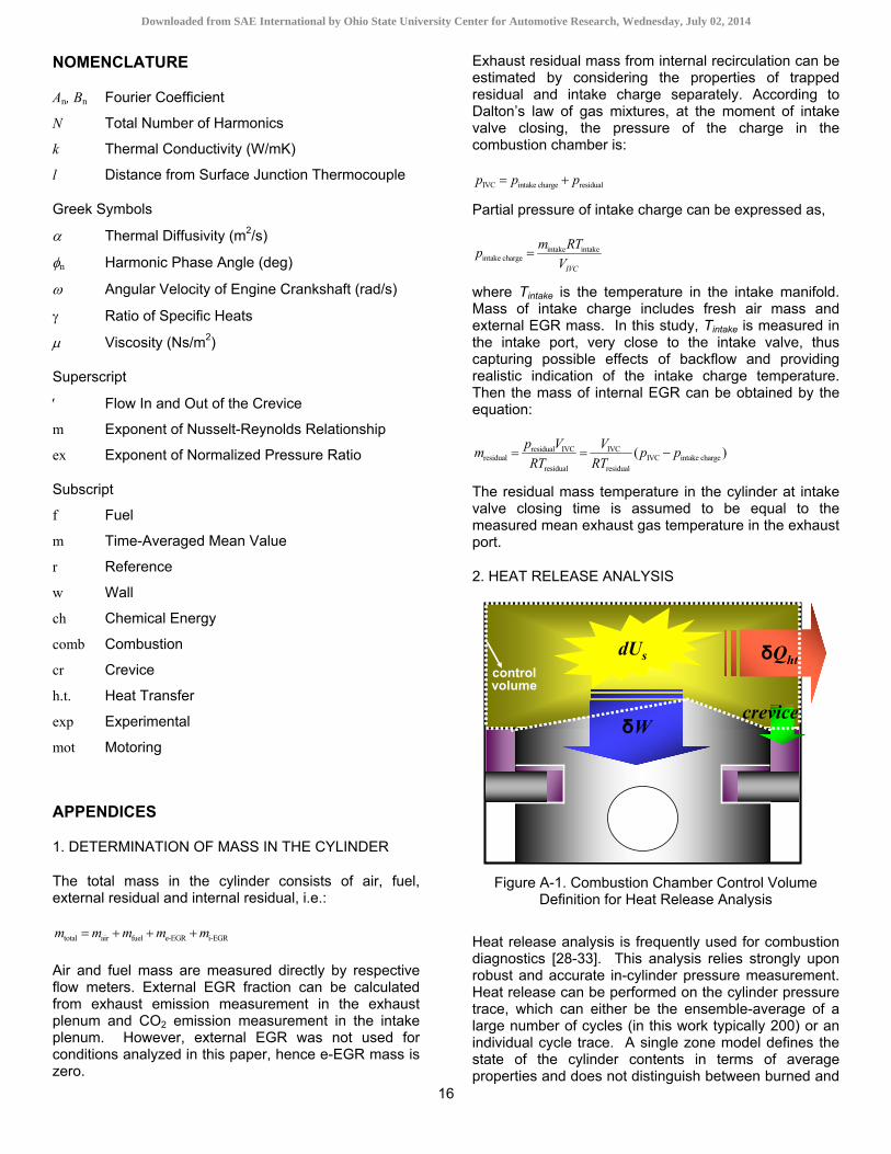

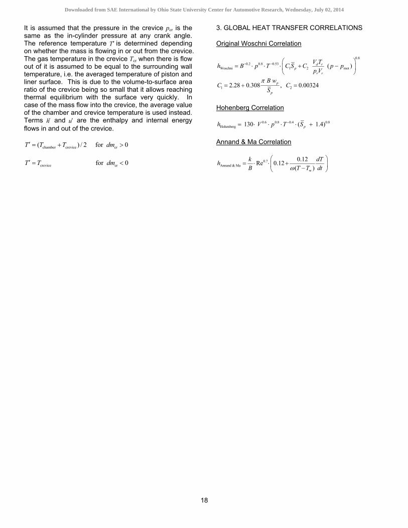


![HCCI - Update of Progress 2005 - US Department of Energy · HCCI – Update of Progress 2005 HCCI HCCI ... M EP [b a r] B S F C [g/k W-hr] ... Typically used in 2-Stroke Engines at](https://static.documents.pub/doc/80x56/5ac4ebc77f8b9a220b8d1053/hcci-update-of-progress-2005-us-department-of-energy-update-of-progress.jpg)


