Page 1
Supplementary Information
Assessing Environmental, Economic, and Reliability Impacts of Flexible
Ramp Products in Midcontinent ISO
Adam Cornelius1, Rubenka Bandyopadhyay2 and Dalia Patiño-Echeverri2, *
1E-mail: [email protected] Federal Energy Regulatory Commission (FERC), Washington, DC. His substantive work on this paper was
performed while a student at Duke University prior to his employment at FERC. The opinions expressed in this paper are those of the authors
only, and do not represent the views of the US Government, FERC, nor of any Commissioners
2 E-mail: [email protected] Nicholas School of the Environment, Duke University, Durham, NC 27708, USA
2E-mail: [email protected] Nicholas School of the Environment, Duke University, Durham, NC 27708, USA.
* Corresponding Author: [email protected] , Phone: 919-358-0858, fax: 919-684-8741
This document contains 23 pages, 21 tables, and one figure.
Page 2
1. Test System Composition
Table S1 shows the fuel mix of the full MISO system and the scaled versions for both wind scenarios.
2009 MISO Full and 6% Scaled Capacity Mix
Coal
NG
Combined
Cycle
NG
Combustion
Turbine
NG
Steam Wind Nuclear Hydro Other Total
2009
MISO
Full
Capacity
(MW) 63682 14864 19872 2951 8103 8508 3407 7577 128962
% of
Total 49% 12% 15% 2% 6% 7% 3% 6% --
Low
Wind
Scenario
Capacity
(MW) 3897 1046 1206 147 526 552 0 0 7374
% of
Total 53% 14% 16% 2% 7% 7% 0% 0% --
High
Wind
Scenario
Capacity
(MW) 3897 1046 1206 147 1585 552 0 0 8433
% of
Total 46% 12% 14% 2% 19% 7% 0% 0% --
Table S1 - Name plate capacity by fuel type of actual 2009 MISO system and our 6% scaled representative
grid under both high and low wind penetration scenarios.
2. Overview of the clustering technique
The eGrid database [1] is used to identify active generators in the MISO region fueled by coal and natural
gas, and their corresponding rated nameplate capacities (NPC) and heat rates (HR). Generators are then
divided into four classes: coal-fired and natural gas combustion cycle (NGCC), natural gas combustion
turbine (NGCT) and natural gas steam generators (NGST).
We do not have sufficient information to model the various stages of NGCC plants; for simplicity, all
generators in NGCC plants are combined and treated as one large generator.
Several outliers from each class are removed to avoid distorting the clusters:
One small coal generator with a very high heat rate (>46,000 Btu/kWh). This heat rate is so
extreme that this generator would become its own cluster, yet would likely never be dispatched.
(Total 2 MW)
Three NGCC generators that are larger than the total NGCC target from Table S1; each has mid-
level heat rates. (Total 4212 MW)
Three NGST generators that were larger than the total NGST target from Table S1; each had mid-
level heat rates. (Total 2218 MW)
One NGST generator with missing heat rate information. (Total 35 MW)
40 NGCT generators with negative heat rates. (1266 MW)
27 NGST generators with extremely high heat rates (>50,000 Btu/kWh). (Total 938 MW)
Heat rates and nameplate capacities are normalized so that values ranged between 0 and 1. Wade’s
clustering technique is implemented for each generator class using Stata software. Wade’s cluster centers
are used as starting points for k-means clustering. A representative generator is selected from each cluster
based on minimum distance from the mean normalized heat rate and mean normalized nameplate capacity
Page 3
of the cluster. For each class of generator, k is chosen such that the total capacity of the representative
generators is as close as possible to the target capacity for that class.
Cluster Number of units
in the cluster
Nameplate Capacity of
Representative Generator (MW)
Heat Rate of Representative
Generator (Btu/kWh)
1 34 114 10527.87
2 32 80 11829.01
3 32 14 11843.46
4 17 25 14225.27
5 4 136 14352.43
6 17 265 11153.35
7 32 180 10858.84
8 17 364 10320.69
9 12 456 10766.79
10 50 13 5263.00
11 28 31 7932.48
12 11 20 23545.42
13 4 25 29645.81
14 16 33 16693.87
15 8 20 19506.04
16 33 574 10529.05
17 6 726 9963.66
18 8 823 9752.89
Table S2 – Clusters corresponding to coal generators.
Cluster Number of units
in the cluster
Nameplate Capacity of
Representative Generator (MW)
Heat Rate of Representative
Generator (Btu/kWh)
1 14 644 7634.34
2 5 66 12267.52
3 4 284 6917.76
4 4 53 8547.36
Table S3 – Clusters corresponding to natural gas combined cycle (NGCC) generators.
Cluster Number of units
in the cluster
Nameplate Capacity of
Representative Generator (MW)
Heat Rate of Representative
Generator (Btu/kWh)
1 6 9 18028.79
2 2 50 13383.17
3 1 82 15004.34
4 13 6 4859.36
Table S4 – Clusters corresponding to natural gas steam (NGST) generators.
Page 4
Cluster Number of units
in the cluster
Nameplate Capacity of
Representative Generator (MW)
Heat Rate of Representative
Generator (Btu/kWh)
1 12 24 11562.50
2 5 18 6268.87
3 37 61 11038.53
4 13 20 15127.12
5 18 18 17395.10
6 17 43 15864.27
7 18 49 18648.90
8 8 17 21708.13
9 14 114 13631.56
10 21 88 12676.84
11 28 91 15675.82
12 11 85 22775.33
13 2 129 23375.26
14 11 18 29633.68
15 2 79 29596.88
16 24 187 11795.45
17 2 166 16358.13
Table S5 – Clusters corresponding to natural gas combustion turbine (NGCT) generators.
3. Operational Parameters
Table S6 summarizes the parameters and corresponding data sources for fossil-fired units in the MISO
Test System
Parameter Unit Description Source Value Comments
Min generation % per MW of
installed
capacity (NPC)
Minimum generator
output level
Coal Plants:
Report by
Renewable
Northwest
Project [2]
PC1 (0-200 MW):
~33% of NPC
PC (200-400
MW): ~40% of
NPC
PC (400-800
MW): ~40% of
NPC
PC (>800): ~40%
of NPC
(Ref: approximate
averages from
table 4 of [2])
NGCC: 40-60%
of NPC
(assuming an
average of 50%)
page 3 of [3],
consistent with a
Siemens report [4]
1 Pulverized Coal (PC) power plant
Page 5
NGCT (<65
MW): 30% of
NPC Page 6 of [5]
NGCT (>=65
MW): 50% of
NPC (Average
value as per
estimates in [6]
and [7]
NGST (0-200
MW) : 30% of
NPC
(approximation
from table 15,
page 97 of [6])
Percentage of
increase in
weekly heat
rates due to one
additional start-
up
% (Primarily) Chemical
energy from fuel
required by generator
at start-up
Power plant
Cycling
Costs by
NREL [8],
Page 47,
Table 1-4
PC (0-299):
0.62%
PC (>300): 0.44%
NGCC: 0.20%
NGCT(<65 MW):
0%
NGCT(>=65
MW): 0.20%
NGST: 0.20%
Start-up C&M
Costs
Start-up
Capitalized
Cycling and
Maintenance
costs ($/ MW
of NPC)
(Capitalized
cycling and
maintenance
costs occur due
to higher non-
routine
maintenance
and capital
replacement
costs as a result
of cycling)
Median
values for
warm start
from Page
12, table 1-1
of [8]
PC (0-299): 157
$/MW
PC (>300): 65
$/MW
NGCC: 55 $/MW
NGCT(>=65):
126 $/MW
NGCT(<65 MW):
24 $/MW
NGST: 58 $/MW
Fixed costs for
start-ups
Auxiliary
power, water
additives etc.
$/MW NPC Table 1-3, pg
30 of NREL
report on
power plant
cycling costs
[8]
PC (0-299): 6.14
$/MW
PC (>300): 7.98
$/MW
NGCC: 3$/MW
[9]
Page 6
NGCT (>=65
MW): 0.95 $/MW
NGCT (<65
MW): 1.90 $/MW
NGST: 6.86
$/MW
No Load Heat-
Rate
MBtu/MW-h Heat input required
when the generator is
kept on-line at zero
load
Analysis
from EPA
AMPD data-
base [10] as
per
instructions
from NLC
calculations
in PJM [11]
PC (0-200 MW):
0.7
PC (200-400): 0.7
PC (400-800):
1.51
PC (>800): 2.28
NGCC: 1.44
NGCT: 1.24
NGST (0-200
MW) : 0.534
Calculated value
roughly in the range
of numbers reported
in [6]
Ramp Rates % NPC/min Max. allowable change
in dispatched power
between two
consecutive intervals
for given generator
during start-up
Report by
European
Local
Electricity
Production
[12], Data
from GE
Website [7]
PC: 3% of NPC
Table 3, pg 22
[12]
NGCC: 5% Table
3, pg 22 [12]
NGCT-
aeroderivate: 20%
Table 3, pg 22
[12]
NGCT- simple
cycle frame: 7.6
% [7]
NGST: 3% Table
3, pg 22 [12]
Min up time hours Minimum time
required for unit to
start up and reach full
load
PJM report
[13]
Coal units: 10 h
NGCC: 5 h
NGST (if
generator came
online after
1985):5 h
NGST (if
generator came
online before
1985):9 h
NGCT (<65
MW): 2 h
NGCT (>=65
MW): 3 h
Min down time hours Minimum time
required for generator
following a shut-down
PJM report
[13]
Coal units: 8 h
NGCC: 4 h
Page 7
needed before starting
up again
NGST (if
generator came
online after
1985):4 h
NGST (if
generator came
online before
1985):7 h
NGCT (<65
MW): 1 h
NGCT (>=65
MW): 3 h
Fuel Prices
$/MBtu EIA database
(Refer to
comments
for exact
citations)
NG: 4.71 $/MBtu
Coal: 2.32 $/Mbtu
Conversion Factor:
$/1000 cubic-
feet=1.028 $/Mbtu
[14]
4.71 $/MmBtu for NG
(average of costs
reported by EIA
between 2009-2014
[15]
NG prices are in
Nominal Dollars
Cost of Coal: 2.32
$/Mbtu based on
average prices
reported in 2009 and
2010 [16]. Assumed
dollar values
corresponding to 2009
and 2010 respectively
Spinning
Reserve Costs
Assumption,
agrees with
assumption
made in a
paper by Liu
et. al [17]
20% of Marginal
Costs
Table S6 – Generators Parameters and Data Sources
Start-up cost calculations:
Start-up costs for each generator are estimated as the sum of Fixed Start-Up costs (Auxiliary power, water
additives etc.), Start-up Capitalized Cycling and Maintenance (C&M) Costs, and the cost of additional
fuel burned to start-up. The additional fuel burned at start-up is estimated from information on the
increased heat rate per one additional start up as reported in [8] –estimated from past studies of various
units and 10 years of hourly EPA Compliance Monitoring System (CMS) database [10]), fuel costs, and
our own estimate of the weekly generation (explained below).
Hence the following equation is used:
Start-Up Cost ($/start-up) = Fixed Start-Up Cost ($) + Start-up Capitalized Cycling & Maintenance Cost
($) + Percentage of increase in weekly heat rates due to one additional start-up (%)*Average Heat Rate
(Btu/kWh)*Average Weekly Generation (kWh)*cost of fuel ($/Btu) (i)
Page 8
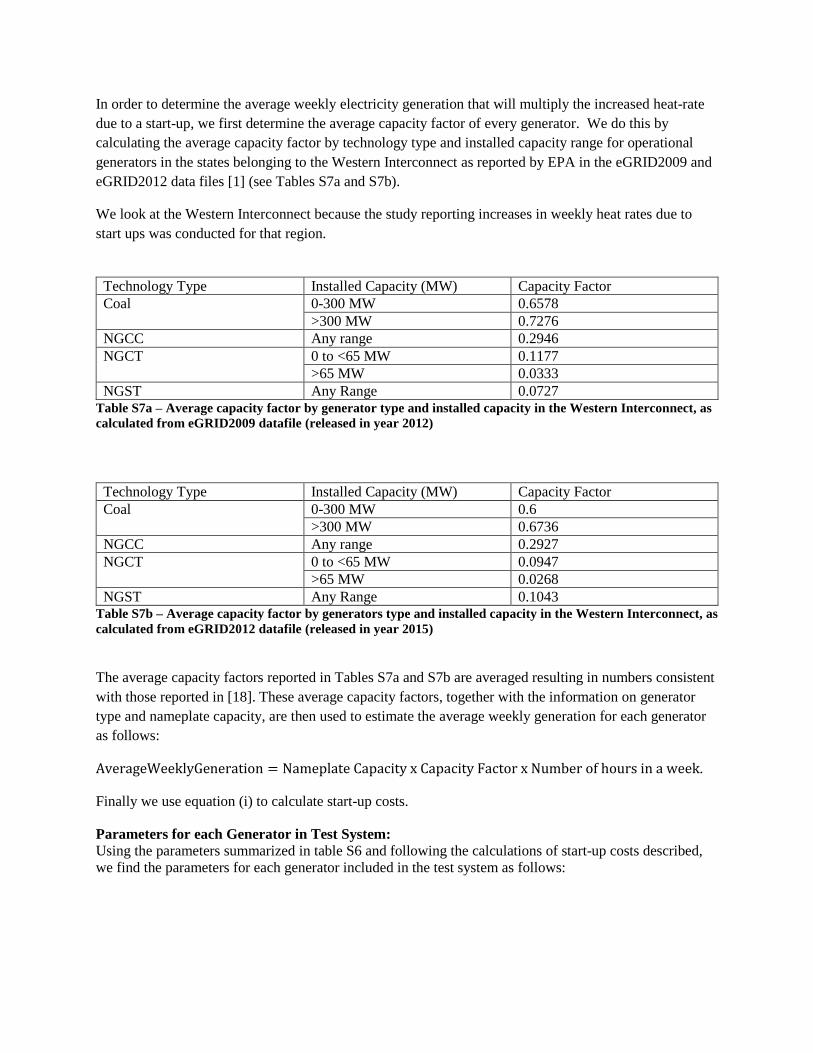
In order to determine the average weekly electricity generation that will multiply the increased heat-rate
due to a start-up, we first determine the average capacity factor of every generator. We do this by
calculating the average capacity factor by technology type and installed capacity range for operational
generators in the states belonging to the Western Interconnect as reported by EPA in the eGRID2009 and
eGRID2012 data files [1] (see Tables S7a and S7b).
We look at the Western Interconnect because the study reporting increases in weekly heat rates due to
start ups was conducted for that region.
Technology Type Installed Capacity (MW) Capacity Factor
Coal 0-300 MW 0.6578
>300 MW 0.7276
NGCC Any range 0.2946
NGCT
0 to <65 MW 0.1177
>65 MW 0.0333
NGST Any Range 0.0727 Table S7a – Average capacity factor by generator type and installed capacity in the Western Interconnect, as
calculated from eGRID2009 datafile (released in year 2012)
Technology Type Installed Capacity (MW) Capacity Factor
Coal 0-300 MW 0.6
>300 MW 0.6736
NGCC Any range 0.2927
NGCT
0 to <65 MW 0.0947
>65 MW 0.0268
NGST Any Range 0.1043 Table S7b – Average capacity factor by generators type and installed capacity in the Western Interconnect, as
calculated from eGRID2012 datafile (released in year 2015)
The average capacity factors reported in Tables S7a and S7b are averaged resulting in numbers consistent
with those reported in [18]. These average capacity factors, together with the information on generator
type and nameplate capacity, are then used to estimate the average weekly generation for each generator
as follows:
AverageWeeklyGeneration = Nameplate Capacity x Capacity Factor x Number of hours in a week.
Finally we use equation (i) to calculate start-up costs.
Parameters for each Generator in Test System: Using the parameters summarized in table S6 and following the calculations of start-up costs described,
we find the parameters for each generator included in the test system as follows:
Page 9
Table S8 – Description of fossil fuel generators in the test system
Nuclear Generators
Nuclear generators represented approximately 7% of MISO nameplate capacity in 2008. In our scaled-
down test grid, there is 552 MW of nuclear capacity. Because most nuclear generators are committed days
in advance and change their output very slowly, we assume that nuclear output is constant at a level
commensurate with its 2009 capacity factor of 84% [1]. We do not include nuclear generators in our
TypeHR
(Btu/kWh)
Max Gen
(MW)
Min Gen
(MW)
Ramp Rate
Up
(MW/Min)
Ramp
Rate down
(MW/Min)
Min
Uptime
(min)
Min
Downtim
e (min)
Gen Cost
($/MWh)
NLC
($/h)
Start-up
Cost ($)
Average
CO_2
emission
rates lb
CO2/MWh
Average
additional
CO_2
Emissions
during start-
up (lb)
Coal 10528.0 113.5 37.5 3.4 3.4 600.0 480.0 24.3 184.2 20330.9 2213.0 1732197.6
Coal 11829.0 80.0 26.4 2.4 2.4 600.0 480.0 27.3 129.8 14488.2 2486.5 1541351.7
Coal 11843.0 13.6 4.5 0.4 0.4 600.0 480.0 27.4 22.1 2463.3 2489.5 262660.3
Coal 14225.0 25.0 8.3 0.8 0.8 600.0 480.0 32.9 40.6 4618.5 2990.2 696575.4
Coal 14352.0 136.0 44.9 4.1 4.1 600.0 480.0 33.2 220.7 25151.1 3016.9 3857376.0
Coal 11153.0 265.2 106.1 8.0 8.0 600.0 480.0 25.8 430.3 47756.3 2344.4 4542405.7
Coal 10859.0 179.5 59.2 5.4 5.4 600.0 480.0 25.1 291.3 32243.6 2282.5 2914425.8
Coal 10321.0 363.8 145.5 10.9 10.9 600.0 480.0 23.8 590.3 31057.9 2169.4 4218500.8
Coal 10767.0 456.0 182.4 13.7 13.7 600.0 480.0 24.9 1596.2 39173.3 2263.2 5754539.3
Coal 5263.0 12.5 4.1 0.4 0.4 600.0 480.0 12.2 20.3 2139.2 1106.3 47675.2
Coal 7932.0 31.0 10.2 0.9 0.9 600.0 480.0 18.3 50.3 5430.7 1667.4 268577.0
Coal 23545.0 20.4 6.7 0.6 0.6 600.0 480.0 54.4 33.1 4057.4 4949.2 1557222.1
Coal 29646.0 25.0 8.3 0.8 0.8 600.0 480.0 68.5 40.6 5204.0 6231.6 3025413.8
Coal 16694.0 33.0 10.9 1.0 1.0 600.0 480.0 38.6 53.5 6220.2 3509.1 1266329.4
Coal 19506.0 19.5 6.4 0.6 0.6 600.0 480.0 45.1 31.6 3758.8 4100.2 1021615.0
Coal 10529.0 574.3 229.7 17.2 17.2 600.0 480.0 24.3 2010.3 49171.9 2213.2 6930742.0
Coal 9964.0 725.8 290.3 21.8 21.8 600.0 480.0 23.0 2540.6 61651.1 2094.4 7843947.0
Coal 9753.0 822.6 329.0 24.7 24.7 600.0 480.0 22.5 4347.8 69665.1 2050.1 8517759.0
NG_CC 7634.0 644.0 322.0 32.2 32.2 300.0 240.0 35.3 4371.4 39638.9 893.2 433349.8
NG_CC 12268.0 65.5 32.8 3.3 3.3 300.0 240.0 56.8 444.6 4172.8 1435.3 113815.4
NG_CC 6918.0 283.5 141.8 14.2 14.2 300.0 240.0 32.0 1924.4 17355.3 809.4 156649.1
NG_CC 8547.0 53.0 26.5 2.7 2.7 300.0 240.0 39.6 359.8 3284.7 1000.0 44704.5
NG_CT 11563.0 23.8 7.1 4.8 4.8 120.0 60.0 53.5 139.1 616.4 1352.8 0.0
NG_CT 6269.0 17.5 5.3 3.5 3.5 120.0 60.0 29.0 102.3 453.3 733.5 0.0
NG_CT 11039.0 61.0 18.3 12.2 12.2 120.0 60.0 51.1 356.6 1579.9 1291.5 0.0
NG_CT 15127.0 20.0 6.0 4.0 4.0 120.0 60.0 70.0 116.9 518.0 1769.9 0.0
NG_CT 17395.0 18.0 5.4 3.6 3.6 120.0 60.0 80.5 105.2 466.2 2035.2 0.0
NG_CT 15864.0 42.9 12.9 8.6 8.6 120.0 60.0 73.4 250.8 1111.1 1856.1 0.0
NG_CT 18649.0 48.6 14.6 9.7 9.7 120.0 60.0 86.3 284.1 1258.7 2181.9 0.0
NG_CT 21708.0 17.3 5.2 3.5 3.5 120.0 60.0 100.5 101.1 448.1 2539.9 0.0
NG_CT 13632.0 114.0 57.0 8.7 8.7 180.0 180.0 63.1 666.3 14546.4 1594.9 25067.0
NG_CT 12677.0 88.2 44.1 6.7 6.7 180.0 180.0 58.7 515.5 11250.3 1483.2 16772.1
NG_CT 15676.0 91.0 45.5 6.9 6.9 180.0 180.0 72.6 531.9 11620.5 1834.1 26460.5
NG_CT 22775.0 85.0 42.5 6.5 6.5 180.0 180.0 105.4 496.8 10883.0 2664.7 52171.5
NG_CT 23375.0 129.0 64.5 9.8 9.8 180.0 180.0 108.2 754.0 16520.3 2734.9 83404.5
NG_CT 29634.0 17.6 5.3 3.5 3.5 120.0 60.0 137.1 102.9 543.6 3467.1 64526.5
NG_CT 29597.0 78.8 39.4 6.0 6.0 180.0 180.0 137.0 460.6 10114.8 3462.8 81679.2
NG_CT 11795.0 187.0 93.5 14.2 14.2 180.0 180.0 54.6 1093.0 23844.8 1380.1 30785.5
NG_CT 16358.0 166.3 83.2 12.6 12.6 180.0 180.0 75.7 972.0 21241.5 1913.9 52656.0
NG_ST 18029.0 9.4 2.8 0.3 0.3 540.0 420.0 83.4 23.7 633.4 2109.4 10630.0
NG_ST 13383.0 50.0 15.0 1.5 1.5 540.0 420.0 61.9 125.9 3336.8 1565.8 31156.7
NG_ST 15004.0 81.6 24.5 2.4 2.4 540.0 420.0 69.4 205.4 5464.2 1755.5 63912.0
NG_ST 4859.0 6.2 1.9 0.2 0.2 540.0 420.0 22.5 15.6 406.4 568.5 509.3
Parameters of fossil-fired units within the MISO test system
Page 10
commitment and dispatch models, but rather subtract this amount (463 MW) from the load in all
intervals.
4. Representation of Wind Generators
EWITS data contains modeled day-ahead hourly forecasts and real-time 10-minute power levels for over
1000 potential wind farm sites throughout the Eastern Interconnection. To choose the sites and scale their
capacity levels, we follow the steps below.
Low Wind Scenario
1. The low wind scenario is based on MISO wind capacity in 2009 as represented in eGRID. Four
MISO states, Iowa, Minnesota, Indiana, and North Dakota had significantly more installed
capacity than other MISO states.
2. We randomly choose a simulated wind farm from each of the four states from the EWITS dataset
and ensure the farm is within MISO territory.
3. We determine a scale value for each wind farm so that the total generation would represent 6% of
2009 levels and the proportion of generation of each farm would roughly match that of its state.
4. We multiply the day-ahead and real-time values by the scale factor for each site and then sum to
get a single set of wind forecasts and real-time generation levels.
High Wind Scenario
1. In the high wind-scenario, wind capacity triples to approximately 19% of total MISO generation
capacity. To achieve this higher level, we assume installation of the same wind farms included in
the low-wind scenario and add an additional randomly-selected EWITS farm from Illinois a state
which by 2013, had the second-most wind in the region [19].
2. Steps 3-4 are the same as above except a new scale factor for each farm is selected to achieve the
higher target of total wind capacity and proportions representing 2013 capacity for each state.
Page 11
Iowa Indiana Minnesota North
Dakota Illinois
System
Total
EWITS Wind farm number 2443 4913 1924 273 7070 --
EWITS Site Latitude 42.573 40.095 44.492 45.966 40.337 --
EWITS Site Longitude -93.643 -86.491 -95.856 -98.964 -91.333 --
EWITS Site Nameplate Capacity (MW) 278 279 295 297 295 --
2009 State Installed Capacity (eGRID) 3,442 1,037 1,603 958 111 8,087
Low Wind Scenario Scale Factor 0.92 0.28 0.41 0.24 -- --
Low Wind Scenario Nameplate Capacity (MW) 256 78 121 71 -- 526
2013 State Installed Capacity (AWEA) (may
include non-MISO area within a state) 5,133 1,543 2,987 1,681 3,568 16,401
High Wind Scenario Scale Factor 1.86 0.56 1.16 0.65 1.29 --
High Wind Scenario Nameplate Capacity (MW) 517 155 340 192 381 1,585
Table S9 – Actual wind nameplate capacity in MISO states in 2009 and 2013 and nameplate capacities of
simulated wind farms in low and high wind scenarios
5. Load Data
We use MISO system load data collected and published by LCG Consulting. Data is missing for
approximately 0.6% of all intervals. These values are estimated using the following method:
1. If a single data point is missing, it is replaced with the average of the intervals directly preceding
and following it.
2. There are two longer time periods of missing data, one lasting for just over 7 hours, and the other
for 35 minutes. In these instances, the missing data is generated using the 5-minute load changes
from the previous day.
We then scale each value down to 6.5% of its original. Table S10 shows minimum, maximum, and
average load for each month after subtracting 463 MW of baseload power contributed by nuclear power
plants over the entire time horizon.
10-minute Load (MW) - Summary Statistics
Min Max Average
January 3,268 5,568 4,563
April 2,799 4,548 3,762
July 3,218 6,779 5,080
Table S10 – Demand summary statistics of each month
6. Forecasts of Wind and Load Data
Both the day ahead and real time markets require forecasts of load and wind power generation. Day-ahead
wind forecasts are provided with the EWITS data. For day-ahead load forecasts, we first find the hourly
real-time load by averaging the loads from the six 10-minute intervals. Next we generate the day ahead
forecast error % by generating a random normal variable with mean 0 and standard deviation 0.01. The
day-ahead forecast is equal to the hourly real time value increased or decreased by a percentage equal to
the randomly generated forecast error, as in (2) below:
Page 12
Define:
h: Index for day-ahead time intervals, ℎ ∈ 1. .24
t: Index for real-time time intervals, 𝑡 ∈ 1. .144
Eh: Day-ahead load forecast error in interval h (%)
FDemandh: Day-ahead forecasted load in interval h (MW)
ActDemandt: Actual real-time demand in interval t (MW)
Day-ahead load forecast generation:
𝐸ℎ~𝑁(0, 0.01) (ii)
𝐹𝐷𝑒𝑚𝑎𝑛𝑑ℎ = (1 + 𝐸ℎ) ∗ 𝐴𝑣𝑒𝑟𝑎𝑔𝑒(𝐴𝑐𝑡𝐷𝑒𝑚𝑎𝑛𝑑6∗ℎ+1, … 𝐴𝑐𝑡𝐷𝑒𝑚𝑎𝑛𝑑6∗ℎ+6) (iii)
A similar procedure is followed for 10-minute wind and load forecasts, using standard deviations of 0.04
and 0.002, respectively.
7. Other Market Clearing Parameters
Other parameters necessary for the StdMC and RCMC models (and summarized in Table S18) are chosen
as follows:
-Spinning Reserve Percentage and Reserve Response Time: MISO currently schedules contingency
reserve of 2,000 MW, all of which must be fully deployed in 10 minutes [20]. This represents about 3.3%
of MISO’s 2009 average load of 61,000 MW and about 2.1% of 2009 peak load of 96,500 MW. In this
paper, we assume the system operator schedules 3.5% of load as spinning reserve in each interval, rather
than the annual average.
-Ramp Response Time and Ramp Intervals: MISO’s proposal targets ramp capability to cover variability
and uncertainty over 10 minutes, or two real-time intervals in their system [21]. Our system uses 10-
minute intervals, so we targeted ramp capability to cover a single real-time interval.
-Over-generation Penalty, Under-generation penalty, Spinning Reserve Scarcity Price: These three
values are penalty prices to ensure that supply and demand remain in balance and that sufficient spinning
reserves are procured if possible. Over-generation penalty is set to $500/MWh based on MISO’s offer
floor of -$500/MWh. This high value makes wind curtailment to be chosen as a balancing mechanism
before allowing an over-generation event. The under-generation penalty is set to MISO’s value of lost
load of $3500/MWh. The spinning reserve scarcity price is set to MISO’s Operating Reserve Demand
Curve Scarcity Price of $1100/MWh [20]. These relative values are such that in intervals with insufficient
generation, the models prioritized meeting energy demand before meeting reserves, which is desirable.
-URC Demand Curve Price and DRC Demand Curve Price: These were based on MISO’s ramp
capability products proposal and were both set at $10 [21]. These prices ensure that ramp capability is
procured if it is inexpensive, and only after energy and spinning reserves requirements are met.
8. Estimation of Flexible Ramp Requirements
Ramp requirement calculations involve the calculation of two components: (a) variability as calculated at
current time interval (given by the difference between actual net load at time t and forecasted net load for
time t+1), and (b) estimation of error in forecasting. The forecast error is expressed as a percent of the
forecast net load and estimated through statistical analysis of the differences between actual and
Page 13
forecasted net load for a historical time series. The same forecast errors (as a percentage of forecast net
load) are used by the day-ahead and real-time models. In order to calculate these, we take the following
steps for both the low and high wind scenarios:
1. Subtract real-time wind generation from real-time load to calculate actual net load for 2009, the
year preceding the modeled year.
2. Subtract forecasted wind generation from forecasted load to calculate forecasted net load for
2009, the year preceding the modeled year.
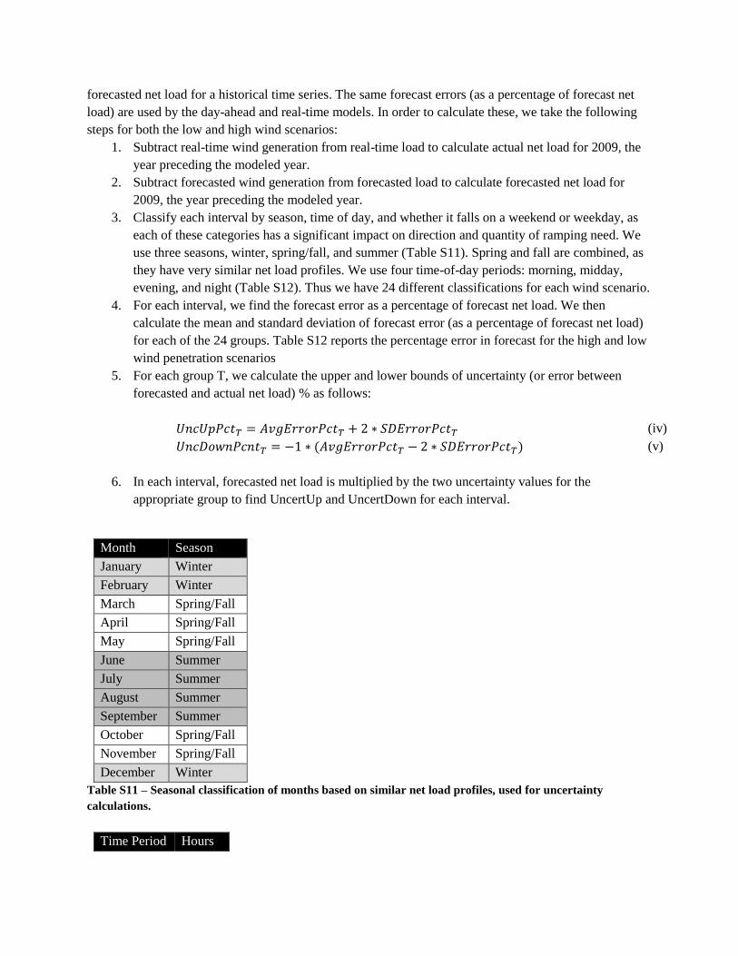
3. Classify each interval by season, time of day, and whether it falls on a weekend or weekday, as
each of these categories has a significant impact on direction and quantity of ramping need. We
use three seasons, winter, spring/fall, and summer (Table S11). Spring and fall are combined, as
they have very similar net load profiles. We use four time-of-day periods: morning, midday,
evening, and night (Table S12). Thus we have 24 different classifications for each wind scenario.
4. For each interval, we find the forecast error as a percentage of forecast net load. We then
calculate the mean and standard deviation of forecast error (as a percentage of forecast net load)
for each of the 24 groups. Table S12 reports the percentage error in forecast for the high and low
wind penetration scenarios
5. For each group T, we calculate the upper and lower bounds of uncertainty (or error between
forecasted and actual net load) % as follows:
𝑈𝑛𝑐𝑈𝑝𝑃𝑐𝑡𝑇 = 𝐴𝑣𝑔𝐸𝑟𝑟𝑜𝑟𝑃𝑐𝑡𝑇 + 2 ∗ 𝑆𝐷𝐸𝑟𝑟𝑜𝑟𝑃𝑐𝑡𝑇 (iv)
𝑈𝑛𝑐𝐷𝑜𝑤𝑛𝑃𝑐𝑛𝑡𝑇 = −1 ∗ (𝐴𝑣𝑔𝐸𝑟𝑟𝑜𝑟𝑃𝑐𝑡𝑇 − 2 ∗ 𝑆𝐷𝐸𝑟𝑟𝑜𝑟𝑃𝑐𝑡𝑇) (v)
6. In each interval, forecasted net load is multiplied by the two uncertainty values for the
appropriate group to find UncertUp and UncertDown for each interval.
Month Season
January Winter
February Winter
March Spring/Fall
April Spring/Fall
May Spring/Fall
June Summer
July Summer
August Summer
September Summer
October Spring/Fall
November Spring/Fall
December Winter
Table S11 – Seasonal classification of months based on similar net load profiles, used for uncertainty
calculations.
Time Period Hours
Page 14
Morning 04 - 09
Midday 10 - 16
Evening 17 - 20
Night 21 - 03
Table S12 – Classification of hourly intervals into time periods based on ramping characteristics, used for
uncertainty calculations.
Uncertainty Percentage of Forecast Error
Low Wind Scenario High Wind Scenario
Season Weekday Day Time Group Uncertainty Up Uncertainty Down Uncertainty Up Uncertainty Down
Winter
Weekend
Morning 1 0.80% -0.81% 2.42% -2.43%
Midday 2 0.76% -0.73% 2.25% -2.25%
Evening 3 0.73% -0.74% 2.23% -2.27%
Night 4 0.86% -0.87% 2.69% -2.63%
Weekday
Morning 5 0.74% -0.72% 2.01% -2.04%
Midday 6 0.69% -0.68% 1.72% -1.76%
Evening 7 0.71% -0.70% 1.97% -1.93%
Night 8 0.84% -0.85% 2.51% -2.52%
Spring/
Fall
Weekend
Morning 9 0.90% -0.93% 3.48% -3.35%
Midday 10 0.86% -0.86% 2.78% -2.72%
Evening 11 0.85% -0.84% 2.81% -2.92%
Night 12 1.00% -0.96% 3.64% -3.58%
Weekday
Morning 13 0.78% -0.77% 2.20% -2.20%
Midday 14 0.73% -0.72% 2.01% -2.03%
Evening 15 0.78% -0.77% 2.50% -2.50%
Night 16 0.91% -0.92% 3.14% -3.11%
Summer
Weekend
Morning 17 0.70% -0.66% 1.50% -1.50%
Midday 18 0.60% -0.58% 1.38% -1.42%
Evening 19 0.61% -0.62% 1.49% -1.44%
Night 20 0.72% -0.73% 2.04% -2.07%
Weekday
Morning 21 0.64% -0.65% 1.48% -1.51%
Midday 22 0.56% -0.55% 1.20% -1.23%
Evening 23 0.61% -0.61% 1.43% -1.46%
Night 24 0.77% -0.77% 2.31% -2.29%
Table S13 – Uncertainty in each direction as a percentage of net load for each of 24 groups in the low and
high wind scenarios
9. Procurement of URC and DRC
Figure S2 illustrates the five possible situations that could occur in any given interval depending on
ramping capability required, baseline levels of ramping capability and the economics of available power
generators. In this example, the demand price is set at $10/MW for all intervals. In this particular interval
for situations 2 – 5, historical analysis has indicated that the system should procure 100 MW of URC.
Page 15
1. For a particular interval, historical analysis could determine that there is a very low likelihood of
a need for any ramp capability and set the target amount to 0 MW.
2. If the system without the ramping constraint would have provided 120 MW anyway, the URC
constraint is non-binding and the price is set at $0/MW.
3. If providing any amount of ramping capability is higher than the price cap, none is procured.
4. If the system wouldn’t naturally provide sufficient URC, but the cost of doing so is relatively low,
the full 100 MW is procured and the price is set below the demand curve value, in this case
$6/MW.
5. If the opportunity cost of providing ramp capability is high, the price is capped at $10/MW which
will limit the amount procured, in this case to 60 MW, leaving a shortage of URC.
Figure S1: Demonstration of the five possible scenarios given a $10/MW URC demand curve price. The
upward-sloping lines represent URC supply curves and the diamond markers indicate the market clearing
quantity and price in each scenario. Scenario 1: Historical analysis determines no URC is needed. Scenario 2:
Historical analysis targets 100 MW of URC. Existing generators provide 120 MW, so no additional URC is
procured; the price is $0/MW. Scenario 3: Historical analysis targets 100 MW of URC. There is insufficient
ramp capability in the system, so the ramp capability constraint is binding. Only some ramp capability is able
to be procured below the $10/MW demand curve price cap, so there is a shortage of URC. Scenario 4:
Historical analysis targets 100 MW of URC. However, the cost to provide any URC is greater than the $10/MW
price cap and therefore none is procured. Scenario 5: Historical analysis targets 100 MW of URC. There is
insufficient ramp capability in the system, so the ramp capability constraint is binding. All 100 MW are able to
be procured for less than the $10/MW demand curve price cap.
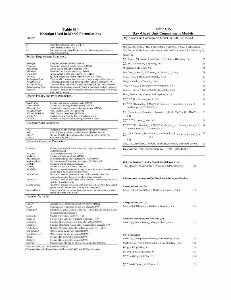
10. Unit Commitment/Economic Dispatch (UC/ED) Models and System Cost Calculations for
the MISO test System
Table S14 defines the variables used for UC-ED modeling, and tables S15-S18 list the problem
formulation for the UC-ED operation of the MISO test system with and without ramp capability products
(StdMC and RCMC models respectively). Table S19 summarizes the parameters used in the baseline
analysis.
0
2
4
6
8
10
12
14
16
18
0 20 40 60 80 100 120 140
Co
st (
$/M
W)
Ramp Capability (MW)
Demand Curve
Scenario 1: No URCtargeted
Scenario 2: Non-bindingURC constraint; noadditional URC procuredScenario 3: No URCprocured; price higherthan demand curveScenario 4: Binding URCconstraint; all targetedURC procuredScenario 5: Binding URCconstraint; shortage ofURC;
Page 17
Table S14
Notation Used in Model Formulations Indices
u
t
n
Index for dispatchable unit, 𝑢 ∈ 1. . 𝑈
Index for time interval, 𝑡 ∈ 1. . 𝑇
Intermediate time interval index used for minimum up and downtime
requirements, 𝑛 ∈ 𝑡..
System Requirement Parameters
IntLength
FDemandt
ActDemandt
Length of each time interval [minutes]
Forecasted system demand in interval t [MW]
Actual system demand in interval t [MW]
VForecastt
VAvailablet
SpinReqt
ResResponseTime
RCUpDCMaxt
RCDownDCMaxt
RampResponseTime
RampInts
Forecasted wind power in interval t [MW]
Actual available wind power in interval t [MW]
Quantity of spinning reserve required in interval t [MW]
Time by which reserve from generator u must be deployable [minutes]
The targeted amount of up-ramp capability (URC) in interval t [MW]
The targeted amount of down-ramp capability (DRC) in interval t [MW]
Response time for ramp capability (used in day-ahead models) [minutes]
Number of intervals for which ramp capability is considered (used in real-
time model) [intervals]
System Penalty and Price Parameters
OverGenPen System-wide over generation penalty [$/MWh] UnderGenPen
SRScarcityPen
RCUpDCPrice*
RCDownDCPrice*
MCPE t *
MCPSRt*
System-wide under generation penalty [$/MWh]
System-wide spinning reserve shortage penalty [$/MWh]
URC Demand Curve Price [$/MWh]
DRC Demand Curve Price [$/MWh]
Market Clearing Price for Energy Market at time t
Market Clearing Price for Spinning Reserves at time t
Generator Cost Parameters
MCu
SRCu
NLCu*
StartCu*
Marginal Cost of operating dispatchable unit u [$/MW/interval]
Cost of spinning reserve provided by unit u [$/MW/interval]
No load cost (fixed operation cost) of operating unit u [$/interval]
Cost of starting unit u [$]
Generator Operating Parameters
Commitu,t
MaxGenu
MinGenu
PosRampRateu
NegRampRateu
MinUTu
MinDTu
InitMinUpu
InitMinDownu
FutureSDu
SUIntsRemainu,t
ShuttingDownu,t
Commitment status of unit u in interval t (only a parameter in economic
dispatch models)
Maximum generation of unit u [MW]
Minimum generation of unit u [MW]
Maximum ramp-up rate of generator u [MW/interval]
Maximum ramp-down rate of generator u [MW/interval]
Minimum uptime of unit u [intervals]
Minimum downtime of unit u [intervals]
Number of intervals generator u must be up at the start of the optimization
period due to its initial uptime [intervals]
Number of intervals generator u must be down at the start of the
optimization period due to its initial downtime [intervals]
Number of intervals beyond the end of the RTED time horizon that unit u
will shut down [intervals]
Number of intervals remaining until generator u should have fully started
up and reached its minimum capacity level [intervals]
Indicates whether the unit is shutting down and the minimum generation
should be relaxed to 0 [binary]
Decision Variables
Genu,t* Average power generation of unit u in interval t [MW]
SRu,t* Spinning reserve provided by unit u in interval t [MW]
Commitu,t#* Commitment status of unit u in interval t (only a decision variable in unit
commitment models) [binary]
StartCostu,t# Startup cost of unit u in interval t [$]
OverGent Surplus of generation over demand in interval t [MW]
UnderGent Shortage of generation below demand in interval t [MW]
UnmetSRt Shortage of spinning reserve below requirement in interval t [MW]
VSchedulet,t Quantity of variable generation scheduled in interval t [MW]
UnitRCUpu,t* URC supplied by unit u in interval t [MW]
UnitRCDownu,t* DRC supplied by unit u in interval t [MW]
RCUpt System URC procured in interval t [MW]
RCDownt System DRC procured in interval t [MW]
Startedu,t* Start-up status of unit u in interval t of a given day d [binary]
* Used for system cost calculations in Table VI
# These decision variables are determined by the B-DAUC and RC-DAUC models
Table S15
Day Ahead Unit Commitment Models
Day Ahead Unit Commitment Model for StdMC (DAUC)
Min ∑ (∑ (Genu,t ∗ MCu + SRu,t × SRCu + Commitu,t × NLCu + StartCostu,t)Uu=1 +T
t=1
OverGent × OverGenPen + UnderGent × UnderGenPen + UnmetSRt × SRScarcityPen)
(1)
Subject to:
∑ Genu,t + VSchedulet + UnderGent − OverGent = FDemandtUu=1 ∀ t (2)
∑ SRu,t + UnmetSRt ≥ SpinReqtUu=1 ∀ t (3)
VSchedulet ≤ VForecastt ∀ t (4)
StartCostu,t ≥ StartCu × (Commitu,t − Commitu,t−1) ∀ u, t (5)
Genu,t + SRu,t ≤ MaxGenu × Commitu,t ∀ u, t (6)
Genu,t ≥ MinGenu × Commitu,t ∀ u, t (7)
Genu,t − Genu,t−1 ≤ IntLength × PosRampRateu ∀ u, t (8)
Genu,t−1 − Genu,t ≤ IntLength × NegRampRateu ∀ u, t (9)
SResu,t ResResponseTime⁄ ≤ PosRampRateu ∀ u, t (10)
∑ (1 − Commitu,t) = 0InitMinUput=1 ∀ u (11)
∑ (Commitu,n) ≥ MinDTu ×t+MinUTu−1n=t (Commitu,t − Commitu,t−1) ∀ u, ∀ t ∈
{InitMinUpu + 1, T − MinUTu + 1}
(12)
∑ (Commitu,n − (Commitu,t − Commitu,t−1)) ≥ 0Tn=t ∀ u, ∀t ∈ {T − MinUTu +
2, T}
(13)
∑ Commitu,t = 0InitMinDownut=1 ∀ u (14)
∑ (1 − Commitu,n) ≥ MinDTu ×t+MinDTu−1n=t (Commitu,t−1 − Commitu,t) ∀ u, ∀ t ∈
{InitMinDownu + 1, T − MinDTu + 1}
(15)
∑ ((1 − Commitu,n) − (Commitu,t−1 − Commitu,t))
≥ 0
Tn=t ∀ u, ∀t ∈ {T − MinDTu +
2, T}
(16)
Genu,t, SRu,t, StartCostu,t, OverGent, UnderGent, UnmetSRt , VSchedulet ≥ 0 ∀u, t (17)
Day Ahead Unit Commitment for RCMC (RC-DAUC)
Objective function is equal to (1) with the additional terms:
− ∑ (RCUpt × RCUpDCPrice + RCDownt × RCDownDCPrice)Tt=1 (18)
All constraints the same as (2)-(17) with the following modifications:
Change to constraint (6):
Genu,t + SRu,t + UnitRCUpu,t ≤ MaxGenu × Commitu,t ∀ u, t (19)
Change to constraint (7):
Genu,t − UnitRCDownu,t ≥ MinGenu × Commitu,t ∀ u, t (20)
Additional components for constraint (17):
UnitRCUpu,t, UnitRCDownu,t, RCUpt, RCDownt ≥ 0 ∀t (21)
New Constraints:
UnitRCUpu,t RampResponseTime⁄ ≤ PosRampRateu ∀ u, t (22)
UnitRCDownu,t RampResponseTime⁄ ≤ NegRampRateu ∀u, t (23)
RCUpt ≤ RCUpDCMaxt ∀t (24)
RCDownt ≤ RCDownDCMaxt ∀t (25)
∑ UnitRCUpu,t ≥ RCUptUnitsu ∀t (26)
∑ UnitRCDownu,t ≥ RCDowntUnitsu ∀t (27)
Page 18
Table S16
Day Ahead Economic Dispatch Models
Day Ahead Economic Dispatch Model for StdMC (B-DAED)
Min ∑ (∑ (Genu,t × MCu + SRu,t × SRCu)Uu=1 + OverGent × OverGenPen + UnderGent ×T
t=1
UnderGenPen + UnmetSRt × SRScarcityPen)
(28)
Subject to:
∑ Genu,t + VSchedulet + UnderGent − OverGent = FDemandtUu=1 ∀ t (29)
∑ SRu,t + UnmetSRt ≥ SpinReqtUu=1 ∀ t (30)
VSchedulet ≤ VForecastt ∀ t (31)
Genu,t + SRu,t ≤ MaxGenu × Commitu,t ∀ u, t (32)
Genu,t ≥ MinGenu × Commitu,t ∀ u, t (33)
Genu,t − Genu,t−1 ≤ IntLength × PosRampRateu ∀ u, t (34)
Genu,t−1 − Genu,t ≤ IntLength × NegRampRateu ∀ u, t (35)
SRu,t ResResponseTime⁄ ≤ PosRampRateu ∀ u, t (36)
Genu,t, SRu,t, OverGent, UnderGent, UnmetSRt, VSchedulet ≥ 0 ∀u, t (37)
Day Ahead Economic Dispatch Model for RCMC (RC-DAED)
Objective function is equal to (28) with the additional terms:
− ∑ (RCUpt × RCUpDCPrice + RCDownt × RCDownDCPrice)Tt=1 (38)
All constraints the same as (29)-(37) with the following modifications:
Change to constraint (32):
Genu,t + SRu,t + UnitRCUpu,t ≤ MaxGenu × Commitu,t ∀ u, t (39)
Change to constraint (33):
Genu,t − UnitRCDownu,t ≥ MinGenu × Commitu,t ∀ u, t (40)
Additional components for constraint (37):
UnitRCUpu,t, UnitRCDownu,t, RCUpt, RCDownt ≥ 0 ∀t (41)
New Constraints:
UnitRCUpu,t RampResponseTime⁄ ≤ PosRampRateu ∀ u, t (42)
UnitRCDownu,t RampResponseTime⁄ ≤ NegRampRateu ∀u, t (43)
RCUpt ≤ RCUpDCMaxt ∀t (44)
RCDownt ≤ RCDownDCMaxt ∀t (45)
∑ UnitRCUpu,t ≥ RCUptUnitsu ∀t (46)
∑ UnitRCDownu,t ≥ RCDowntUnitsu ∀t (47)
Table S17
Real Time Economic Dispatch Models
Real Time Economic Dispatch Model for StdMC (B-RTED)
The objective function is the same as that in B-DAED
All constraints the same as (29)-(37) with the following modifications:
Constraint (29) is replaced with:
∑ Genu,t + VSchedulet + UnderGent − OverGent = ActDemandtUu=1 ∀ t
(48)
Constraint (31) is replaced with:
VSchedulet ≤ VAvailablet ∀ t (49)
Constraint 33 is replaced with:
Genu,t ≥ (MinGenu × Commitu,t − SUIntsRemainu,t ∗ PosRampRateu ∗
IntLength) ∗ (1 − ShuttingDownu,t) ∀ u, t
(50)
New Constraint
Genu,t ≤ (FutureSDu + T − t) × IntLength × NegRampRateu ∀ u, (51)
Real Time Economic Dispatch for RCMC (RC-RTED)
The objective function is the same as that in RC-DAED
All constraints the same as 39-47 with the following modifications:
Constraint (39) is replaced with:
∑ Genu,t + VSchedulet + UnderGent − OverGent = ActDemandtUu=1 ∀ t (52)
Constraint (31) is replaced with:
VSchedulet ≤ VAvailablet ∀ t (53)
Constraint (40) is replaced with:
Genu,t ≥ (MinGenu × Commitu,t − SUIntsRemainu,t ∗ PosRampRateu ∗
IntLength) ∗ (1 − ShuttingDownu,t) ∀ u, t
(54)
Change to constraint (42):
UnitRCUpu,t RampInts ∗ IntLength⁄ ≤ PosRampRateu ∀ u, t (55)
Change to constraint 43
UnitRCDownu,t RampInts ∗ Intlength⁄ ≤ NegRampRateu ∀u, t (56)
New Constraints:
Genu,t + UnitRCUpu,t ≤ (FutureSDu + T − t) × IntLength × NegRampRateu ∀ u, t (57)
Page 19
Table S18
Parameters used in baseline analysis
Variable Name Description B-DAUC/ B-
DAED
B-RTED RC-DAUC/
RC-DAED
RC-RTED
T # Intervals in Time
Horizon [intervals]
24 1 24 1
IntLength Length of each interval
[minutes]
60 10 60 10
SpinPercentage % of load required for
spinning reserve
3.5 3.5 3.5 3.5
ResResponseTime time by which spinning
reserve must be
deployable [minutes]
10 10 10 10
RampResponseTime Response time for ramp
capability [minutes]
-- -- 10 --
RampInts # intervals for which
ramp capability is
considered [intervals]
-- -- -- 1
OverGenPen Over generation penalty
[$/MWh]
500 500 500 500
UnderGenPen Under generation penalty
[$/MWh]
3,500 3,500 3,500 3,500
SRScarcityPen System-wide spinning
reserve shortage penalty
[$/MWh]
1,100 1,100 1,100 1,100
RCUpDCPrice URC Demand Curve
Price [$/MWh]
10 10 10 10
RCDownDCPrice DRC Demand Curve
Price [$/MWh]
10 10 10 10
11. Additional results
Tables S19, S20 and S21 expand Table 3 in the manuscript to report additional metrics of the economic,
reliability and environmental performance of RCMC. As discussed in the manuscript, under base case
assumptions, RCMC results in reduced emissions, shortage intervals, prices, and costs relative to StdMC
(sensitivity case 0, tables S17-S18). If the URC/DRC price caps are augmented to $15/MWh, the
improvement from RCMC is magnified for all performance metrics and all months (sensitivity case 1).
The only exception is the difference in the average MCP during intervals without energy or reserve
shortages, but this is a partial indicator whose significance is muted by the fact that the difference in
overall prices indicates a greater advantage of RCMC with the URC/DRC prices of this sensitivity case.
Page 20
TABLE S19
COSTS CALCULATIONS FROM OUTPUTS OF STDMC AND
RCMC
StdMC
Generator Costs for unit u during day d (𝐆𝐂𝐮,𝐝)=
∑ (Genu,tRTED × MCu + SRu,t
RTED × SRCu + Commitu,tDAUC × NLCu + Startedu,t
DAUC ×t∈d
StartCu)
(58)
Generator Market Revenue (𝐆𝐌𝐑𝐮,𝐝)=
∑ (Genu,tDAED × MCPEt
DAED + max(Genu,tRTED−Genu,t
DAED , 0) × MCPEtRTED + SRu,t
DAED ×t∈d
MCPSRtDAED + max(SRu,t
RTED − SRu,tDAED , 0) × MCPSRt
RTED
(59)
Generator Uplift Revenue (𝐆𝐔𝐑𝐮,𝐝)=
Max{(GCu,d − GMRu,d),0}
(60)
Generator Total Revenue 𝐝𝐮𝐫𝐢𝐧𝐠 𝐚 𝐝𝐚𝐲(𝐆𝐓𝐑𝐮,𝐝)=
GMRu,d + GURu,d
(61)
Uplift Payments to All Generators in month m (𝐓𝐔𝐆𝐦)=
∑ ∑ (GURu,d)u∈Ud∈m
(62)
Total Payments to All Generators in month m (𝐓𝐏𝐆𝐦)=
∑ ∑ (GMRu,d + GURu,d)u∈Ud∈m
(63)
RCMC
Equation (59) is modified to include the additional terms:
+ ∑ (UnitRCUPu,tDAED × RCUpDCPrice + max(UnitRCUPu,t
RTED − UnitRCUPu,tDAED, 0) ×T
t=1
RCUpDCPrice + UnitRCDownu,tDAED × RCDownDCPrice +
max(UnitRCDownu,tRTED−UnitRCDownu,t
DAED , 0) × RCDownDCPrice)
(64)
*Superscripts ‘DAUC’,’DAED’ and ‘RTED’ represent results from the
corresponding models (e.g. Genu,tDAED represents the average power
generation of unit u during time interval t per the day ahead economic
dispatch model).
Page 21
Table S20 – Relative changes in costs and prices
Table S21 – Relative changes in emissions and reliability metrics
Jan Apr Jul Jan Apr Jul Jan Apr Jul Jan Apr Jul Jan Apr Jul
Base 61.12 98.75 176.15 434 435 483 0.59 0.47 0.48 57.77 64.48 35.98 -1.42 -1.56 -1.95
1 125.50 156.62 316.46 463 438 500 0.65 0.64 0.50 61.73 77.46 66.46 -2.25 -2.12 -3.01
2 11.68 74.38 60.00 295 333 357 0.45 0.34 0.47 11.90 5.39 13.85 -0.66 -0.95 -0.99
3 61.53 237.11 169.18 453 254 525 0.50 0.29 0.63 71.15 71.65 43.49 -1.42 -1.47 -1.74
4 83.21 93.46 218.69 433 353 538 0.67 0.45 0.58 110.61 75.95 42.78 -1.40 -1.66 -1.97
5 67.06 107.28 222.88 375 386 527 0.67 0.34 0.64 84.72 79.51 41.23 -1.47 -1.54 -1.91
Results are differences between standard and flexiramp models with same assumptions
(StdMC - FlexRMC) for high wind scenarios
Case
System Costs (Million
USD)
Revenue Sufficiency
Guarantee Payments
Average Market Clearing Price
($/MWh)
No. of
instances of
payment
Payment
(Million USD)Overall
Non-shortage
Intervals
Improvement
more than base
Improvement less
than the base case
Deterioration less
than base case
Deterioration more
than the base case
Improvement due to Ramp Capability
Pricing
Deterioration due to Ramp Capability
Pricing
Legend
Jan Apr Jul Jan Apr Jul Jan Apr Jul Jan Apr Jul
Base 8.77 9.76 7.59 43 40 11 78 110 100 11.85 12.89 15.70
1 11.28 10.22 9.62 63 60 21 128 124 186 17.23 18.47 32.45
2 3.18 9.28 4.57 22 30 11 6 22 45 1.11 1.59 7.70
3 8.13 55.13 6.74 48 39 17 114 53 126 17.36 15.13 20.41
4 8.37 54.43 6.72 46 34 9 127 50 95 18.01 13.40 16.24
5 14.16 49.62 8.95 35 33 12 179 113 255 18.11 16.88 15.47
No. of
Generator
Start-ups
Reserve Scarity
Results as differences between standard and ramp capability pricing models
with same assumptions (StdMC-FlexRMC) for high wind scenarios
Case
CO2 Emissions (in
1000 Short tons)Number of
Instances
Reserve Scarcity in
1000 MW
Improvement
more than base
Improvement less
than the base case
Deterioration less
than base case
Deterioration more
than the base case
Improvement due to Ramp Capability
Pricing
Deterioration due to Ramp Capability
Pricing
Legend
Page 22
References
[1] Environmantal Protection Agency, "eGrid Database," 2014. [Online]. Available: http://www.epa.gov/cleanenergy/energy-resources/egrid/.
[Accessed 26 April 2015].
[2] J. Lindsay and K. Dragoon, "Summary Report on Coal Plant Dynamic Performance Capability," Renewable Northwest Project, 2010.
[3] National Energy Technology Laboratory, "Impact of Load Following on Power Plant Cost and Performance," 2012.
[4] L. Balling, "Flexible future for combined cycle," December 2010. [Online]. Available: http://www.energy.siemens.com/hq/pool/hq/power-
generation/power-plants/gas-fired-power-plants/combined-cycle-powerplants/Flexible_future_for_combined_cycle_US.pdf. [Accessed 20
November 2015].
[5] Wartsila and Energy Exemplar, "Power System Optimization by increased flexibility," 2014.
[6] A. Mills and R. Wiser, "Changes in the Economic Value of Variable Generation at High Penetration Levels," Ernest Orlando Lawrence
Berkeley National Laboratory, 2012.
[7] General Electric, "7E.03 GAS TURBINE," [Online]. Available: https://powergen.gepower.com/content/dam/gepower-
pgdp/global/en_US/documents/product/gas%20turbines/Fact%20Sheet/7e03-fact-sheet-april-2015.pdf. [Accessed 21 November 2015].
[8] Intertek APTECH, "NREL Power Plant Cycling Costs".
[9] G. Brinkman, "Renewable Electricity Futures: Operational Analysis of the Western Interconnection at Very High Renewable Penetration,"
National Renewable Energy Laboratory , 2015.
[10] US Environmental Protection Agency, "Air Markets Program Data," [Online]. Available: http://ampd.epa.gov/ampd/. [Accessed 11
November 2015].
[11] PJM, "No Load Definition: Educational Document," 2011.
[12] J. Klimstra, "On the values of local electricity generation," European Local Electricity Production, 2007.
[13] J. Bowring, "Updated Operating Parameter matrix," 2007. [Online]. Available:
http://www.monitoringanalytics.com/reports/Presentations/2007/011107-rmwg.pdf. [Accessed 20 November 2015].
[14] US Energy Information Agency, "What are Ccf, Mcf, Btu, and therms? How do I convert natural gas prices in dollars per Ccf or Mcf to
dollars per Btu or therm?," [Online]. Available: https://www.eia.gov/tools/faqs/faq.cfm?id=45&t=8. [Accessed 30 November 2015].
[15] US Energy Information Agency, "Natural Gas Prices," [Online]. Available: http://www.eia.gov/beta/dnav/ng/ng_pri_sum_dcu_nus_a.htm.
[Accessed 30 November 2015].
[16] US Energy Information Administration Agency, "Coal Data Browser," [Online]. Available:
http://www.eia.gov/beta/coal/data/browser/?src=-
f4#/topic/23?agg=0,1&geo=g&sec=vs&freq=A&start=2008&end=2013&ctype=map<ype=pin&rtype=s&pin=&rse=0&maptype=0.
[Accessed 30 November 2015].
Page 23
[17] G. Liu and K. Tomsovic, "A full demand response model in co-optimized energy and reserve market," Electric Power System Research,
vol. 111, pp. 62-70, 2014.
[18] US Energy Information Administration, " Capacity Factors for Utility Scale Generators Primarily Using Fossil Fuels, January 2013-August
2015," [Online]. Available: http://www.eia.gov/electricity/monthly/epm_table_grapher.cfm?t=epmt_6_07_a. [Accessed 24 November
2015].
[19] American Wind Energy Association, "Wind Energy Facts at a Glance," 2014. [Online]. Available:
http://www.awea.org/Resources/Content.aspx?ItemNumber=5059. [Accessed 4 April 2015].
[20] Midwest Independent System Operator, "Business Rules Governing Contingency Reserve Provided by Batch-Load Demand Response,"
2013. [Online]. Available: https://www.misoenergy.org/_layouts/MISO/ECM/Redirect.aspx?ID=146463. [Accessed 10 July 2016].
[21] N. Navid and G. Rosenwald, "Ramp Capability Product Design for MISO Markets," 2013.
[22] Northwest Powe and Conservation Council, "Sixth Northwest Conservation and Electric Power Plan," 1 February 2010. [Online].
Available: https://www.nwcouncil.org/energy/powerplan/6/plan.
[23] CRA International, "Economic Impact of Eliminating Pancaked Transmission Rates between Entergy and SPP," 2009. [Online]. Available:
http://www.spp.org/publications/cra%20spp-entergy%20rate%20pancaking%20study.pdf.
[24] A. M. a. R. Wiser, "Changes in th Economic Value of Variable Generation at High Penetration Levels," June 2012. [Online]. Available:
http://emp.lbl.gov/sites/all/files/lbnl-5445e.pdf.
[25] N. K. e. al., "NREL Power Plant Cycling Costs," April 2012. [Online]. Available: http://wind.nrel.gov/public/wwis/aptechfinalv2.pdf.
[26] Energy Information Administration, "Carbon Dioxide Emissions Coefficients," 14 February 2013. [Online]. Available:
http://www.eia.gov/environment/emissions/co2_vol_mass.cfm.
[27] Energy Information Administration, "Average Heat Content by State and Region, Electric Power Sector, March 2009-March 2014," 2014.
[Online]. Available: http://www.eia.gov/beta/coal/data/browser.