Assessing the potential for beneficial diversification in rain-fed agricultural enterprises1

John Kandulu2

Abstract

Climate change and climate variability induce uncertainty in yields, and thus

threaten long term economic viability of rain-fed agricultural enterprises. Enterprise

mix diversification is the most common, and is widely regarded as the most

effective, strategy for mitigating multiple sources of farm business risk. We assess

the potential for enterprise mix diversification in mitigating climate induced

variability in long term net returns from rain-fed agriculture. We build on APSIM

modelling and apply Monte Carlo simulation, probability theory, and finance

techniques, to assess the potential for enterprise mix diversification to mitigate

climate-induced variability in long term economic returns from rain-fed agriculture.

We consider four alternative farm enterprise types consisting of three non-diversified

farm enterprises and one diversified farm enterprise consisting of a correlated mix of

rain-fed agricultural activities. We analyse a decision to switch from a non-

diversified agricultural enterprise with the highest expected return to a diversified

agricultural enterprise consisting of a mix of agricultural enterprises. Correlation

analysis showed that yields were not perfectly correlated (i.e. are less than 1)

indicating that changes in climate variables cause non-proportional impacts on yield

production. We conclude that at best, diversification can reduce the standard

deviation of net returns by up to about A$110 Ha-1, or 52% of mean net returns;

increase the probability of below-average net returns by up to about 4% and increase

the mean of 10% of worst probable annual net returns by up to A$54/ha. At worst,

diversification can reduce the mean of net returns by up to about A$95 Ha-1, or 46%.

Keywords: climate variability; yield uncertainty; economic returns; rain-fed

agricultural enterprise, risk, Monte Carlo

1. Introduction 1 A contributed paper to the 55th Annual Conference of the Australian Agricultural and Resource Economics Society, Feb 9-11, 2011, Melbourne Convention Centre, Melbourne, VIC. 2 CSIRO Ecosystem Sciences, john.kandulu@csiro.au

Australia’s major agricultural regions are characterised by uncertain and variable

climatic conditions including temperature and rainfall (Furuya and Kobayashi, 2009;

Wang et al., 2009a). Climate variability is the principal source of risk affecting long

term economic viability of rain-fed agricultural systems (Marton et al., 2007;

Iglesias and Quiroga, 2007; Lotze-Campen, 2009). Climate models predict an

increase in future climate variability and a significant increase in the frequency of

below-average rainfalls and above-average temperatures in major agricultural

regions in Australia (IPCC 2007; Naylor et al., 2007; Suppiah et al., 2007). All else

being equal, this is likely to increase the uncertainty and variability in agricultural

yields and economic returns, and increase the frequency with which these are below

average (John et al., 2005; Wang et al., 2009b). Consequently, the viability of farm

businesses will become increasingly threatened in the long run.

To manage the severity of the impact of climate variability on net returns, farmers

routinely adopt mitigation strategies involving various adjustments in enterprise mix,

and production technologies and techniques (Kelkar et al., 2008). The diversification

of farm enterprise mixes through the rotation of several different crops and livestock

(hereafter simply diversification), is widely regarded as the most common and

effective strategy for mitigating climate-induced variability in net returns from rain-

fed agriculture (Amita, 2006; Correal etal., 2006; Azam-Ali, 2007). Diversification

can also reduce frequencies of below-average net returns under climate uncertainty

(Bernhau, 2007).

Most of the benefit of diversification comes from hedging against market input and

commodity price fluctuations (Bhende and Venkataram, 1993; Singh, 2000;

Ramaswami et al., 2003; World Bank, 2004). Notwithstanding variance in market

input costs and commodity prices (Hazel et al., 1990; Ramaswami et al., 2003),

climate-induced yield variability is a significant source of farm business risk. We

propose that diversification may also be beneficial for hedging against climatic

variability.

The benefits of diversification are premised on the utilization of imperfectly

correlated net returns from multiple agricultural enterprises. When the impacts of

climatic variability differ between multiple agricultural enterprises, losses from

investments in some activities are offset by gains, or moderated by less severe

losses, in other activities thereby reducing the impact on overall net returns

(Ramaswami et al., 2003; Fraser et al., 2005). Conversely, the benefits of

diversification typically come at a cost of reduced expected net returns (Markowitz’s

1952; Chan et al., 1998). This is because diversification involves investing in

multiple activities to mitigate long term uncertainty and variability even when

investments in alternative non-diversified enterprises may offer higher expected net

returns in the short term (Cooper et al., 2008). As such, the nature and strength of

correlated yields across alternative agricultural activities need to be fully understood

and quantified when assessing the potential benefits of agricultural diversification.

There is a general consensus from the finance literature that not considering the

nature and strength of correlated yields may under- or over-estimate the benefit of

diversification (Markowitz 1952, 1959; Merton, 1980; Chan et al., 1998, 1999;

Bangun et al 2006).

Few studies have considered long term sources of uncertainty and risk such as

climate, and assessments of enterprise mix diversification as a strategy for mitigating

climate risks to ensure long term viability of farm businesses are sparse. Lien and

Hardaker (2009) speculate that this is because relevant historical data necessary for

long term analyses are usually sparse and that most studies have had to rely on a few

observations of economic returns. However, in the context of increasingly frequent

droughts in many of the worlds agricultural regions (Howden et al., 2007; IPCC

2007; Furunya and Kobayashi, 2009; Lotze-Campen and Schellnhuber, 2009), the

impact of diversification on avoiding high cost of crop failure in the long term bears

significant relevance.

In this study, we assessed the potential for enterprise mix diversification to mitigate

climate-induced variability in long-term economic net returns from rain-fed

agriculture. Using a case study in the 11.8 million hectare Lower Murray region in

southern Australia, we fitted probability density functions to modelled long term

crop and livestock yield data. We used Monte Carlo simulation to quantify the

variability in yields and, via a profit function, net returns. We quantified the benefits

and costs of enterprise mix diversification using techniques from finance theory

including the probability of break-even and conditional value at risk (CVaR). We

quantified the trade-off between the reduced variability in returns and reduced

expected net returns, and discuss the implications of diversification as an adaptation

strategy for farmers to cope with increasing climatic variability.

2. Methods

2.1. Study area

The Lower Murray region (Figure 1) in southern Australia covers a total area of

11,871,363 ha. Mean annual rainfall ranges from 200 mm/yr in the drier northern

areas of the SAMDB to 1,400 mm/yr in the southern Wimmera. Rain-fed agriculture

is the dominant land use covering over 50% of the region and is an important

component of the regional economy (Bryan et al. 2007). The average farm size used

for rain-fed agriculture in the study area is around 1,000ha. Farming systems vary

greatly across the region depending on climate and soil types. The cropping of

cereals (wheat, barley), pulses (lupins, beans, peas), and sheep grazing are typical

farm enterprises. Cropping and grazing rotations vary over the region from

continuous cropping in the Wimmera and southern Mallee regions, crop/pasture

rotations in the Mallee and southern SAMDB regions, and continuous grazing in the

central and northern SAMDB (Bryan et al., 2011). Most farmers engage in some

form of annual crop/livestock rotation for a number of reasons including protection

of crops from diseases, management of weeds, diversification, and response to

economic opportunities.

Insert Figure 1 about here

2.2. Modelled farming systems

We modelled and compared yield and economic outcomes for three non-diversified

farming systems and one diversified farming system in the study area. The three

non-diversified farming systems were defined as continuous single-crop farming

systems of wheat, lupins, and sheep grazing on modified pastures (hereafter, sheep).

The diversified farming system was defined as a mixed enterprise comprising

continuous cropping (and grazing) of wheat, lupins, and sheep in equal proportions

of available farmland in any one year production horizon. We controlled for effects

of land management on yields thereby ensuring that variability in yields can be

largely attributed to variability in climate.

2.3. Crop yield modelling

We used the Agricultural Production Simulator (APSIM, Keating et al. 2003) to

predict annual yields for wheat, lupins, and sheep for 138 unique soil/climate zones

over 116 years. The soils/climate zones were identified by overlaying a layer

defining 15 soil types (Bryan et al. 2007) and a layer defining 16 climate zones. The

15 soil types were classified using field-derived soil survey data. Climate zones were

defined by overlaying climate variables including mean annual rainfall, mean annual

temperature, and annual moisture index layers. Soil/climate zones were assumed to

have homogeneous production potential for the purposes of this study. Historical

daily climate records were acquired for the 116-year period from 1889 to 2005 from

the SILO data base. Typical land management regimes (sowing windows, fertiliser

application rates) were defined for the study area based on expert opinion. For full

details and other applications of this modelling we refer readers to Bryan et al.

(2007, 2008, 2009, 2010, 2011.) and Wang et al. (2009). Of the 138 zones modelled

across the entire region, we selected one zone to illustrate results from our

assessment of the potential for beneficial diversification.

2.4. Quantifying climate-induced yield variability

To assess benefits from diversification, we treated annual net returns as stochastic.

This is premised on the assumption that climate, the key variable driving yield

variability which is the focus of our study, is generally assumed to be stochastic

(Iglesias and Quiroga, 2007; Furunya and Kobayashi, 2009). Probability theory

provides a suitable framework for the quantification of climate-driven uncertainty

and variability in net returns over a given time horizon (Hardaker et al., 2004; Lien

and Hardaker, 2009).

We generated frequency histograms for yields Q1i, for each of the three enterprises i,

where i is an element of I{wheat, lupins, sheep}. We then fitted probability density

functions to the frequency histograms to characterize climate-induced variability in

yield outputs using the @RISK software. A total of 414 probability density functions

were fitted to frequency histograms of the three enterprises in 138 APSIM zones

across the region. We used the chi-squared statistics, χ2, to measure the goodness of

fit of each distribution (Iglesias and Quiroga, 2007) using the standard Equation 1.

( ) 22

1

ki i

i i

N EE

χ=

−= ∑ Equation 1

Where k is the number of discrete intervals in a histogram derived from 117 years of

simulated yield time-series data; Ni is the frequency of observations in each interval;

and Ei is the expected (theoretical) frequency, asserted by the estimated probability

density function.

The distribution with the best fit as measured by the chi-squared statistic was

selected for use in Monte Carlo simulation of net economic returns.

2.5. Quantifying variability in economic returns

To fully account for the effect of climate variability on economic net returns from

rain-fed agriculture in the study area, we quantified variability in long term average

net revenue per hectare (Kurukulasuriya, 2007; Deressa, 2009; Bryan et al., 2009)

while controlling for all other economic factors including costs of production and

commodity prices after Benhin (2008). We defined economic net returns as revenues

from sale of commodities produced less the fixed and variable cost incurred in the

production of agricultural commodities. We used a profit function to calculate net

economic net returns for wheat, lupins and sheep such that:

NRi= (P1i×Q1i×TRNi) + (P2i×Q2i ×Q1i)−((QCi×Q1i)+(ACi+FDCi+FOCi+FLCi)) Equation 2

Net returns to the diversified farm enterprise system, NRd. were calculated as:

3

i

d

NRNR

⎛ ⎞⎜ ⎟⎝ ⎠=∑

∈i {wheat, lupins, sheep} Equation 3

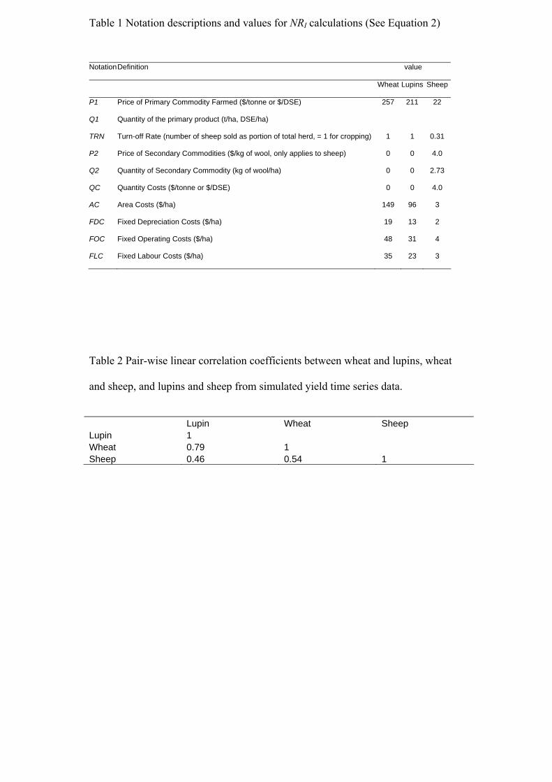
Table 1 outlines notation descriptions and values used in Equation 2 (Bryan et al.,

2009). The profit function has been found to provide a reasonable estimate of

economic returns to agriculture (Bryan et al., 2011).

Insert Table 1 about here

The benefits of diversification in relation to climatic variability rely on imperfect

correlation between yields of crops and grazing systems (Correal et al., 2006;

Iglesias and Quiroga, 2007). Hence, it is important to quantify yield correlations and

include these in simulation of net returns. We calculated pair-wise Pearson

correlation coefficients for yields ρi,i between wheat and lupins, wheat and sheep,

and lupins and sheep from the modelled yield data.

To quantify climate-induced variability in net returns for each land use, NRi, we

generated 1000 Monte Carlo simulations (Hardaker and Lien, 2010) of net returns

using Equation 2 with random samples for the yield parameter Q1i, drawn from the

modelled probability density functions for yields. To quantify climate-induced

variability in net returns for the diversified farm enterprise system, NRd, we

generated 1000 Monte Carlo simulations (Hardaker and Lien, 2010) of net returns

using Equation 2 with random samples for the yield parameter Q1i drawn from the

modelled probability density functions for yields, and considering yield correlations

ρi,i. Frequency histograms were then developed for the average of net returns under

the three non-diversified enterprises and under the diversified enterprise (see

Equation 3).

2.6. Quantifying potential benefits from diversification

To assess the benefits of diversification, we considered farmers in the study area as

investors faced with the challenge of choosing among four alternative farm

enterprises with uncertain net returns. Financial risk management literature offers

various measures for assessing potential tradeoffs between expected net returns and

overall variability in net returns. Specifically, the concept of Conditional Value at

Risk or CVaR (Rockafellar and Uryasev, 1999, 2001) has been used to assess

variability of net returns and probabilities of low-end net returns from alternative

investments. One way to apply CVaR is to calculate the average expected return of

the lowest 10% of possible outcomes (Rockafellar and Uryasev, 1999; 2001).

We used four indicators to quantify the expected net returns and variability of net

returns from each of the four alternative investment options. We calculated the mean

to indicate the magnitude of expected returns, standard deviation to indicate the

variation in expected returns. To estimate magnitudes and probability of below

average economic returns under each of the four options, we calculated the

probability of breaking even P (NRi,d ≥ 0) and the CVaR of the lowest 10% CVaR0.1.

3. Results

We present results from one APSIM zone out of the 138 APSIM zones that we

modelled for purposes of illustration. This area lies in the moderate to high rainfall

region with annual rainfall ranging between 500 and 800mm. We selected this area

because it represents 50th percentile productive capacity for lupins, wheat and

pasture grazing across the region.

3.1. Climate-induced yield variability

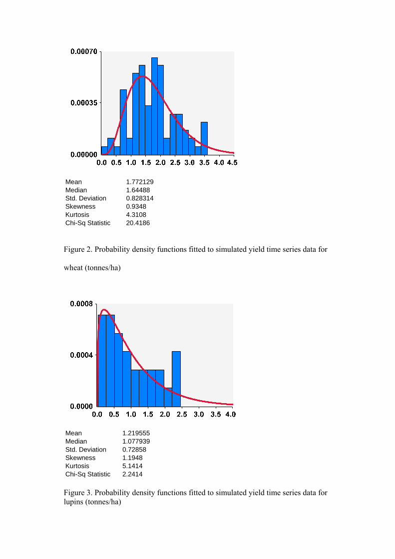
Figures 2, 3, and 4 show how the probability density functions were fitted to

frequency histograms generated from 117 years simulated yield time series data for

wheat, lupins and pasture respectively.

Insert figures 2, 3, and 4 about here

Three probability density functions of various forms were fitted and Chi square

statistics from goodness of fit tests (Equation 1) ranged from 2.2 to 20.4. In all cases,

observed frequencies (counts) were not significantly different from the frequencies

that would be expected using the fitted probability density functions, and estimates

from the probability density function were consistent with observed data from

frequency distributions 90% of the time.

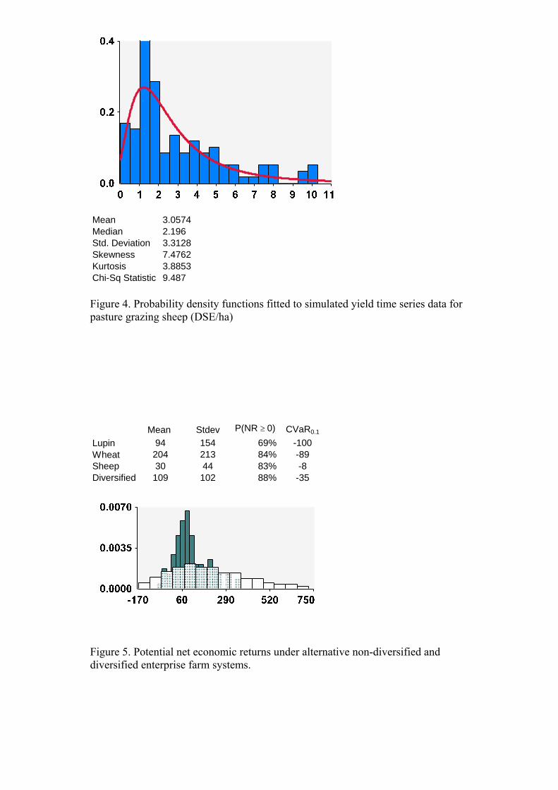
Figures 2, 3, and 4 show that overall, expected yields for lupins are lower than those

for wheat, and yields are lowest and most variable for pasture grazing sheep. Yields

of 1.77 for wheat; 1.22 for lupins; and 3.06 tonnes ha-1 would be expected on

average in the illustrative area. Figures 2, 3, and 4 also shows that variability,

measured using standard deviation, was estimated at 0.82 tonnes ha-1, or 46% of

mean for wheat; 0.73 tonnes ha-1, or 60% of mean for lupins; and 3.31 tonnes ha-1, or

108% of mean for sheep.

3.2. Correlations

In Table 2 we outline pair-wise Pearson correlation coefficients calculated for yields

ρi,i between wheat and lupins, wheat and sheep, and lupins and sheep from the

modelled yield data for our illustrative APSIM zones. Overall, yields are strongly

positively correlated for all land used with highest positive correlations between 0.46

and 0.79. The correlation matrix in table 2 shows that yields are not perfectly

correlated (i.e. are less than 1) in all the cases. We can deduce, therefore, that there is

scope for beneficial diversification in the region.

3.3. Variability in economic net returns

Figure 5 shows that the relative orders of magnitude for the four economic indicators

are highly varied across the four farm enterprise systems.

Insert figure 5 about here

Overall, sheep has lowest expected net returns of all enterprises at A$30 ha-1,

followed by lupins at $94 ha-1, and wheat has highest mean net returns at A$204 ha-

1. The expected net return from the diversified enterprise is A$109 ha-1. All the

three non-diversified enterprises have higher values for standard deviation, as a

proportion of mean, than the diversified enterprise. Lupin has the highest value at

163% of mean; followed by sheep at 146% of mean; then wheat at 104% of mean.

The diversified enterprise has the lowest standard deviation at or 95% of mean.

The probability of breaking even, P (NR ≥ 0), is highest under the diversified

enterprise at 88%, and is lowest for lupins at 69%. For sheep and wheat, P (NR ≥ 0)

is 84% and 84% respectively. The value of the mean of 10% of worst probable

annual net returns, CVaR0.1, is lowest under lupins at. That is, a loss of $100 ha-1on

average would be expected 10% of the time. The CVaR0.1 for wheat is -A$89 ha-1;

and for the diversified enterprise, CVaR0.1 is estimated at -A$35 ha-1. Sheep has the

highest CVaR0.1 at -A$8 ha-1.

3.4. Benefits of diversification

To assess potential benefits from diversification, we consider a decision to switch

from a highest expected return non-diversified farm enterprise system to the

diversified farm enterprise system in ach of the nine locations. In Figure 5, the

highest expected return non-diversified farm enterprise system is wheat.

Figure 5 shows that there is potential for beneficial diversification and there may be

a case for considering a decision to switch from wheat to the diversified farm

enterprise system. Whilst wheat is estimated to have the highest expected net returns

at A$204 ha-1, wheat also has the most variable net returns with standard deviation

values estimated at 104% of mean. In this location, the decision to switch to the

diversified farm enterprise system is estimated to result in lower net returns than

wheat at A$109 ha-1 however, the variability in net returns, standard deviation,

would also be lower at 94%. In switching to a diversified farm enterprise system,

expected returns would be reduced 46%, but the orders of magnitude of standard

deviations of net returns would be reduced even more, by 52%. Further, the

probability of break even will be increased by 4%, and the value of CVaR0.1 is

estimated to increase by about 61%. The diversified enterprise benefits from a

combination of risk-reducing characteristics of sheep, and high expected return

characteristics of wheat. Together these characteristics moderate losses in years with

unfavourable climate to compensate for high-return and high-variability properties

of wheat and reduce the likelihood of extremely low net returns.

4. Discussion

Using a case study in the Lower Murray region in southern Australia, we have

demonstrated the potential for beneficial diversification as a strategy for mitigating

the impacts of climate-driven variability in net returns from investments in rain-fed

agriculture. Enterprise mix diversification can be beneficial and we quantified the

trade off between the benefit of reduced variability and the cost of reduced expected

net returns. To compare the impacts of climate variability with and without

diversification, we quantified variability, expected net returns, and probability and

severity of below-average net returns across the alternative diversified and non-

diversified agricultural investment options taking explicit account of correlations

between yields.

Our study findings are consistent with findings from previously cited studies that

state that there is potential for beneficial diversification from investments in multiple

agricultural activities that respond differently to variability in climate.

Table 2 shows that yields are imperfectly correlated as different activities respond

differently to variability in climate in the study location. Our findings are also

consistent with the expectation that the benefit of reduced variability from

diversification comes at a cost of reduced expected net returns when alternative non-

diversified activities offer higher expected net returns.

At best, diversification can reduce the standard deviation of net returns by up to

about A$110 Ha , or 52% of mean net returns (see Figure 5); increase the

probability of below-average net returns by up to about 4% and increase the value of

CVaR0.1 by orders of magnitude of up to about A$54/ha. At worst, diversification

can reduce the mean of net returns by up to about A$95 Ha , or 46%.

However, there are some limitations to this study. First, only equal proportions of

combinations of 3 investments with equal allocations, 0.33ha, are considered in the

diversified investment option. Whilst this is sufficient for answering key questions

raised in this study, this is not an exhaustive list of possible strategies and may be

suboptimal as it may represent an over (under) investment in some activities

depending on individual’s risk-return preferences. A logical extension to this study

-1

-1

would be to look at more systematic ways of determining optimal diversifications

strategies taking into account risk profiles of farmers (Pannell et al 2000).

The main reason farmers diversify is to hedge against short term variability in input

and commodity price (Kingwell, 1994; Pannell et al 2000; Barkely and Peterson,

2008; Cooper et al., 2008; Lien and Hardaker, 2009) .This study holds these and

other sources of risk except yield, constant to assess the potential for enterprise mix

diversification to mitigate climate-induced variability in long-term economic net

return only to the extent that these are affected by variability in yields. Future studies

may build on this study and explore relative importance of all key sources of farm

income risk to assess potential for beneficial diversification considering multiple

sources of farm business risk.

Further, our study used historical time series data and therefore assumes that

historical climate patterns will continue into future. The impact of climate change on

net returns from yields and the effectiveness of diversification in mitigating

variability in long term net returns from agriculture will vary depending on

assumptions about future climate change. Future climate variability and uncertainty

in climate and yields is assumed to be partly based on historical data however, there

is need to use other information and judgments to improve the relevance of the

results. As an extension to this study, several climate scenarios may be considered in

assessment of potential for beneficial diversification. Subjective probabilities

capturing effects of climate change on future climate variability can be used to

incorporate the effects of climate change in the assessment (Hardaker and Lien,

2010).

Further strategies for adapting to future climate change might involve including

other enterprises with less correlated yields in the diversification of farm enterprise

systems. Specifically, there are new opportunities to diversify farm enterprise

through provision of ecosystem services to benefit from emerging eco-markets (for

example through management of remnant native vegetation, agro forestry for carbon

and biodiversity markets) increase the potential for beneficial diversification as a

strategy for mitigating climate-induced income risk.

5. Conclusion

Diversified farming systems offer farmers a potential strategy for hedging against

climatic risk in economic returns. In the context of increasing climate variability and

frequency of droughts in many of the worlds agricultural regions (Howden et al.,

2007; IPCC 2007; Furunya and Kobayashi, 2009; Lotze-Campen and Schellnhuber,

2009), and emerging markets for ecosystem services, diversification may grow in

significance and relevance as a strategy for avoiding high cost of crop failure and

managing long term farm income risk.

6. Reference List

Amita, S. (2006) Changing interface between agriculture and livestocks: A study of

livelihood options under dry land systems in gujarat. Working Paper - Gujarat

Institute of Development Research, Ahmedabad, 25 pp.

Azam-Ali, S. (2007) Agricultural diversification: The potential for underutilised

crops in africa's changing climates. Rivista Di Biologia-Biology Forum 100, 27-37.

Bangun, P., Nasution, AH., Mawengkang, H (2006) Evaluating Covariance and

Selecting the Risk Model for Asset Allocation. IMT-GT Regional Conference on

Mathematics, Statistics and Applications Universiti Sains Malaysia, Penang, June

2006

Benhin, J.K.A. (2008) South african crop farming and climate change: An economic

assessment of impacts. Global Environmental Change-Human and Policy

Dimensions 18, 666-678.

Bhende, M.J., Venkataram, J.V. (1994) Impact of diversification on household

income and risk - a whole-farm modeling approach. Agricultural Systems 44, 301-

312.

Bryan, B.A., Crossman, N.D., King, D., McNeill, J., Wang, E., Barrett, G., Ferris,

M.M., Morrison, J.B, Pettit, C., Freudenberger, D., O’Leary, G., Fawcett, J., and

Meyer, W. (2007) Lower Murray Landscape Futures Dryland Component: Volume 3

– Preliminary Analysis and Modelling. CSIRO Water for a Healthy Country, 378.

http://www.landscapefutures.com.au/reports/LMLF_Volume3_Dryland_Report_Dat

a_Modelling.pdf

Bryan, B.A., Hajkowicz, S., Marvanek, S., Young, M.D. (2009) Mapping economic

returns to agriculture for informing environmental policy in the murray-darling

basin, Australia. Environmental Modeling & Assessment 14, 375-390.

Bryan, B.A., King, D., Wang, E. (2010) Biofuels agriculture: landscape-scale trade-

offs between fuel, economics, carbon, energy, food, and fiber. Global Change

Biology – Bioenergy 2, 330-345.

Bryan, B.A. King, D., and Ward, J. (2011) Modelling and mapping agricultural

opportunity costs to guide landscape planning for natural resource management.

Ecological Indicators 11, 199-208.

Chan, L.K.C., Karceski, J., Lakonishok, J. (1998) The risk and return from factors.

Journal of Financial and Quantitative Analysis 33, 159-188.

Chan, L.K.C., Karceski, J., Lakonishok, J. (1999) On portfolio optimization:

Forecasting covariances and choosing the risk model. Review of Financial Studies

12, 937-974.

Cooper, P.J.M., Dimes, J., Rao, K.P.C., Shapiro, B., Shiferaw, B., Twomlow, S.

(2008) Coping better with current climatic variability in the rain-fed farming systems

of sub-saharan africa: An essential first step in adapting to future climate change?

Agriculture Ecosystems & Environment 126, 24-35.

Correal, E., Robledo, A., Rios, S., Rivera, D., (2006) Mediterranean dryland mixed

sheep-cereal systems. Sociedad Espanola para el Estudio de los Pastos (SEEP), pp.

14-26.

Deressa, T.T., Hassan, R.M. (2009) Economic impact of climate change on crop

production in ethiopia: Evidence from cross-section measures. Journal of African

Economies 18, 529-554.

Fraser, E.D.G., Mabee, W., Figge, F. (2005) A framework for assessing the

vulnerability of food systems to future shocks. Futures 37, 465-479.

Furuya, J., Kobayashi, S. (2009) Impact of global warming on agricultural product

markets: Stochastic world food model analysis. Sustainability Science 4, 71-79.

Hardaker, J.B., Huirne, R.B.M., Anderson, J.R., Lien, G. (2004) Coping with risk in

agriculture. Coping with risk in agriculture, xii + 332 pp.

Hardaker, J.B., Lien, G. (2010) Probabilities for decision analysis in agriculture and

rural resource economics: The need for a paradigm change. Agricultural Systems

103, 345-350.

Howden, S.M., Soussana, J.F., Tubiello, F.N., Chhetri, N., Dunlop, M., Meinke, H.

(2007) Adapting agriculture to climate change. Proceedings of the National

Academy of Sciences of the United States of America 104, 19691-19696.

Iglesias, A., Quiroga, S. (2007) Measuring the risk of climate variability to cereal

production at five sites in spain. Climate Research 34, 47-57.

IPCC (2007) Climate Change 2007: Synthesis. Summary for policy makers. Fourth

Assessment Report of the Intergovernmental Panel on Climate Change, Cambridge

University Press, Cambridge

John, M., Pannell, D., Kingwell, R. (2005) Climate change and the economics of

farm management in the face of land degradation: Dryland salinity in western

Australia. Canadian Journal of Agricultural Economics-Revue Canadienne D

Agroeconomie 53, 443-459.

Keating, B.A., Carberry, P.S., Hammer, G.L., Probert, M.E., Robertson, M.J.,

Holzworth, D., Huth, N.I., Hargreaves, J.N.G., Meinke, H., Hochman, Z., McLean,

G., Verburg, K., Snow, V., Dimes, J.P., Silburn, M., Wang, E., Brown, S., Bristow,

K.L., Asseng, S., Chapman, S., McCown, R.L., Freebairn, D.M., Smith, C.J. (2003)

An overview of apsim, a model designed for farming systems simulation. European

Journal of Agronomy 18, 267-288.

Kelkar, U., Narula, K.K., Sharma, V.P., Chandna, U. (2008) Vulnerability and

adaptation to climate variability and water stress in uttarakhand state, india. Global

Environmental Change-Human and Policy Dimensions 18, 564-574.

Kingwell, R.S. (1994) Risk attitude and dryland farm-management. Agricultural

Systems 45, 191-202.

Kurukulasuriya, P., Ajwad, M.I. (2007) Application of the ricardian technique to

estimate the impact of climate change on smallholder farming in sri lanka. Climatic

Change 81, 39-59.

Ladanyi, M. (2008) Risk methods and their applications in agriculture. Applied

Ecology and Environmental Research 6, 147-164.

Lien, G., Hardaker, J.B., van Asseldonk, M., Richardson, J.W. (2009) Risk

programming and sparse data: How to get more reliable results. Agricultural

Systems 101, 42-48.

Lotze-Campen, H., Schellnhuber, H.J. (2009) Climate impacts and adaptation

options in agriculture: What we know and what we don't know. Journal Fur

Verbraucherschutz Und Lebensmittelsicherheit-Journal of Consumer Protection and

Food Safety 4, 145-150.

Ludwig, F., Milroy, S.P., Asseng, S. (2009) Impacts of recent climate change on

wheat production systems in western Australia. Climatic Change 92, 495-517.

Magombeyi, M.S., Taigbenu, A.E. (2008) Crop yield risk analysis and mitigation of

smallholder farmers at quaternary catchment level: Case study of b72a in olifants

river basin, south africa. Physics and Chemistry of the Earth 33, 744-756.

Markowitz, H.M. (1952a) Portfolio Selection. Journal of finance, 7, 77-91.

Markowitz, H.M. (1952b) Portfolio Selection: Efficient diversification of

investments. Yale University Press, New Haven, CT.

Markowitz, H.M. (1994) The general mean-variance portfolio selection problem.

Philosophical Transactions of the Royal Society of London Series a-Mathematical

Physical and Engineering Sciences 347, 543-549.

Marton, L., Pilar, P.M., Grewal, M.S. (2007) Long-term studies of crop yields with

changing rainfall and fertilization. Agrartechnische Forschung-Agricultural

Engineering Research 13, 37-47.

Merton, R.C. (1980) On estimating the expected return on the market - an

exploratory investigation. Journal of Financial Economics 8, 323-361.

Naylor, R.L., Battisti, D.S., Vimont, D.J., Falcon, W.P., Burke, M.B. (2007)

Assessing risks of climate variability and climate change for indonesian rice

agriculture. Proceedings of the National Academy of Sciences of the United States

of America 104, 7752-7757.

Pannell, D.J., Malcolm, B., Kingwell, R.S. (2000) Are we risking too much?

Perspectives on risk in farm modelling. Agricultural Economics 23, 69-78.

Ramaswami, B., Ravi, S., Chopra, SD (2003) Risk Management in Agriculture.

Discussion Papers in Economics 03-08. Indian Statistical Institute, Delhi Planning

Unit

Rockafellar, R.T., Uryasev, S. (2002) Conditional value-at-risk for general loss

distributions. Journal of Banking & Finance 26, 1443-1471.

Suppiah, R., Preston, B., Whetton, P H., McInnes, K L., Jones, R N., Macadam, I.,

Bathols J., Kirono D (2006) Climate change under enhanced greenhouse conditions

in South Australia: An updated report on: Assessment of climate change, impacts

and risk management strategies relevant to South Australia. CSIRO regional climate

change report for SA Gov.

Thomas, R.J. (2008) Opportunities to reduce the vulnerability of dryland farmers in

central and west asia and north africa to climate change. Agriculture Ecosystems &

Environment 126, 36-45.

Uryasev, S., Rockafellar, R.T., (2001) Conditional value-at-risk: Optimization

approach, in: Uryasev, S.P., Pardalos, P.M. (Eds.), Stochastic optimization:

Algorithms and applications. Springer, Dordrecht, pp. 411-435.

Wang, E., Cresswell, H., Bryan, B., Glover, M., King, D. (2009a) Modelling farming

systems performance at catchment and regional scales to support natural resource

management. Njas-Wageningen Journal of Life Sciences 57, 101-108.

Wang, E.L., McIntosh, P., Jiang, Q., Xu, J. (2009b) Quantifying the value of

historical climate knowledge and climate forecasts using agricultural systems

modelling. Climatic Change 96, 45-61.

World Bank (2004) Agricultural Diversification for the Poor Guidelines for

Practitioners. March 2004 http://siteresources.worldbank.org/INTARD/825826-

1111044795683/20460111/Diversification_Web.pdf (Accessed 22.10.10)

Table 1 Notation descriptions and values for NRI calculations (See Equation 2)

Notation Definition value

Wheat Lupins Sheep

P1 Price of Primary Commodity Farmed ($/tonne or $/DSE) 257 211 22

Q1 Quantity of the primary product (t/ha, DSE/ha)

TRN Turn-off Rate (number of sheep sold as portion of total herd, = 1 for cropping) 1 1 0.31

P2 Price of Secondary Commodities ($/kg of wool, only applies to sheep) 0 0 4.0

Q2 Quantity of Secondary Commodity (kg of wool/ha) 0 0 2.73

QC Quantity Costs ($/tonne or $/DSE) 0 0 4.0

AC Area Costs ($/ha) 149 96 3

FDC Fixed Depreciation Costs ($/ha) 19 13 2

FOC Fixed Operating Costs ($/ha) 48 31 4

FLC Fixed Labour Costs ($/ha) 35 23 3

Table 2 Pair-wise linear correlation coefficients between wheat and lupins, wheat

and sheep, and lupins and sheep from simulated yield time series data.

Lupin Wheat Sheep Lupin 1 Wheat 0.79 1 Sheep 0.46 0.54 1

Figure 1. Location and land use in the Lower Murray study area.

Mean 1.772129Median 1.64488Std. Deviation 0.828314Skewness 0.9348Kurtosis 4.3108Chi-Sq Statistic 20.4186

Figure 2. Probability density functions fitted to simulated yield time series data for

wheat (tonnes/ha)

Mean 1.219555Median 1.077939Std. Deviation 0.72858Skewness 1.1948Kurtosis 5.1414Chi-Sq Statistic 2.2414 Figure 3. Probability density functions fitted to simulated yield time series data for lupins (tonnes/ha)

Mean 3.0574Median 2.196Std. Deviation 3.3128Skewness 7.4762Kurtosis 3.8853Chi-Sq Statistic 9.487 Figure 4. Probability density functions fitted to simulated yield time series data for pasture grazing sheep (DSE/ha)

Mean Stdev P(NR ≥ 0) CVaR0.1

Lupin 94 154 69% -100Wheat 204 213 84% -89Sheep 30 44 83% -8Diversified 109 102 88% -35

Figure 5. Potential net economic returns under alternative non-diversified and diversified enterprise farm systems.