Assessment and Evaluation of Sand Control Methods for … · Assessment and Evaluation of Sand...

IMPERIAL COLLEGE LONDON

Department of Earth Science and Engineering

Centre for Petroleum Studies

Assessment and Evaluation of Sand Control Methods for a North Sea Field

by

Amir Latiff

A report submitted in partial fulfilment of the

requirements for the MSc and/or the DIC

September 2011

2 Assessment and Evaluation of Sand Control Methods for a North Sea Field

DECLARATION OF OWN WORK

I declare that this thesis Assessment and Evaluation of Sand Control Methods for a North Sea Field

is entirely my own work and that where any material could be construed as the work of others, it is

fully cited and referenced, and/or with appropriate acknowledgement given.

Signature:...................................................................................................................

Name of student: Amir Latiff

Name of Supervisors: Craig Paveley, Nexen Inc.

Robert Zimmerman, Imperial College

Assessment and Evaluation of Sand Control Methods for a North Sea Field 3

CONFIDENTIALITY AGREEMENT

In accordance with the data confidentiality agreement, the actual field and well names are treated as

confidential. For the purpose of reporting, the field would be referred to as “Case Study”, the

reservoirs as “Sand 1 and Sand 2” and the wells as “I1 and I2” for Water Injectors in Sand 1 and

Sand 2, respectively.


ACKNOWLEDGEMENTS

First and foremost, I would like to thank Craig Paveley and Robert Zimmerman for the guidance and advice throughout this

MSc project. My utmost gratitude also goes out to Martin Beesley, Iain Coates and Julien Hailstone; without whose support

this project would not have been possible. I am grateful to Nexen Petroleum U.K. Limited for their sponsorship and guidance,

and for enabling this project to take place. I would also like to say a special thank you to the course director Alain Gringarten

for the knowledge and experience I have gained in the past twelve months. Finally, I would like to thank my parents and my

girlfriend for their consistent support and financing throughout this course.


TABLE OF CONTENTS

DECLARATION OF OWN WORK ................................................................................................................................... 2 CONFIDENTIALITY AGREEMENT ............................................................................................................................... 3 ACKNOWLEDGEMENTS ................................................................................................................................................ 4 TABLE OF CONTENTS .................................................................................................................................................... 5 LIST OF FIGURES ............................................................................................................................................................ 6 LIST OF TABLES .............................................................................................................................................................. 7 ABSTRACT ....................................................................................................................................................................... 8 INTRODUCTION .............................................................................................................................................................. 8 METHODOLOGY: SAND CONTROL SELECTION ...................................................................................................... 9

Flowchart A – ‘First Pass’ Selection Criteria ................................................................................................................. 9 Flowchart B – ‘Screen and Gravel Size’ Selection Criteria. ......................................................................................... 11 Sand Control Selection Table. ...................................................................................................................................... 11

RESULTS: VERIFICATION OF METHODOLOGY ...................................................................................................... 13 Case Study – North Sea Field, UK ............................................................................................................................... 13

Background. .............................................................................................................................................................. 13 Injection Strategy. ..................................................................................................................................................... 13

Rock Mechanics and In-Situ Stresses. .......................................................................................................................... 13 Particle Size Distribution (PSD). .................................................................................................................................. 14

Sand 1. ...................................................................................................................................................................... 16 Sand 2 ....................................................................................................................................................................... 16

Formation Heterogeneity. ............................................................................................................................................. 17 Shale and Zonal Isolation ......................................................................................................................................... 17 Permeability Variation .............................................................................................................................................. 17

Split Injection Rate and Annular Flow ......................................................................................................................... 18 CONCLUSIONS .............................................................................................................................................................. 22 SUGGESTIONS FOR FURTHER WORK ...................................................................................................................... 22 NOMENCLATURE.......................................................................................................................................................... 22 REFERENCES ................................................................................................................................................................. 23 APPENDICES .................................................................................................................................................................. 24

APPENDIX A: CRITICAL LITERATURE MILESTONES TABLE ......................................................................... 25 APPENDIX B: CRITICAL LITERATURE REVIEWS .............................................................................................. 26 API 58-066, 1958 ......................................................................................................................................................... 26 Journal of Petroleum Technology, September 1969 ..................................................................................................... 27 SPE 39437, 1998 .......................................................................................................................................................... 28 SPE 85504, June 2003 .................................................................................................................................................. 29 SPE 88493, October 2004 ............................................................................................................................................. 30 SPE 106018, April 2007 ............................................................................................................................................... 31 SPE 107539, June 2007 ................................................................................................................................................ 32 SPE 112283, February 2008 ......................................................................................................................................... 33 SPE 114781, October 2008 ........................................................................................................................................... 34 SPE 128038, February 2010 ......................................................................................................................................... 35 SPE 137057, November 2010 ....................................................................................................................................... 36 APPENDIX C: NOMENCLATURE ............................................................................................................................ 37 APPENDIX D: METHODOLOGY .............................................................................................................................. 38 APPENDIX E: CASE STUDY BACKGROUND ........................................................................................................ 40 APPENDIX F: SANDING FAILURE PREDICTION ................................................................................................. 42 APPENDIX G: PARTICLE SIZE DISTRIBUTION ................................................................................................... 45 APPENDIX H: FORMATION CONDITION AND SHALE ...................................................................................... 52 APPENDIX I: INJECTION SPLIT RATIO AND ANNULAR FLOW ....................................................................... 55 APPENDIX J: iPoint 2011 (Perigon Solutions) ........................................................................................................... 66 APPENDIX K: NETool

TM 5000.0.0.0 (Landmark) ...................................................................................................... 67


LIST OF FIGURES Figure 1: Flowchart A is used as ‘First Pass Selection Criteria’ for both openhole and cased hole wells. ....................... 10 Figure 2: Flowchart B represents ‘Screen and Gravel Size Selection’. ............................................................................ 12 Figure 3: Section of Well Est1 wireline log from 9330 to 9440ft MD (Reservoir 1). The Formation Image (FMI) and

caliper logs show no evidence of borehole breakouts and washouts respectively. ........................................................... 14 Figure 4: Large variation in fines for Sand 1 show LPSA gives accurate measurement of fines below 44μm. ............... 14 Figure 5: Large variation in fines for Sand 2 show LPSA gives accurate measurement of fines below 44μm. ............... 15 Figure 6: Particle Size Distribution (PSD) of Sand 1 using DSA and LPSA combined (Beesley et al. 2011). ................ 15 Figure 7: Particle Size Distribution (PSD) of Sand 2 using DSA and LPSA combined (Beesley et al. 2011). ................ 15 Figure 8: Schematic showing Uc and Fines of Sand 1 within the methodology boundaries to use SAS. ........................ 16 Figure 9: Schematic showing Uc and Fines of Sand 2 also within the methodology boundaries to use SAS. ................. 16 Figure 10: Permeability and porosity relationship of Sand 1 in the horizontal and vertical direction. ............................. 17 Figure 11: Permeability and porosity relationship of Sand 2 in the horizontal and vertical direction. ............................. 18 Figure 12: Vertical-to-horizontal permeability ratio (KV/KH) in Sand 1 is more anisotropic than Sand 2. ...................... 18 Figure 13: Schematic shows the KV/KH in Sand 2 is less anisotropic compared to Sand 1. ............................................. 19 Figure 14: NETool

TM shows Barefoot and SAS completions matches. ............................................................................ 19

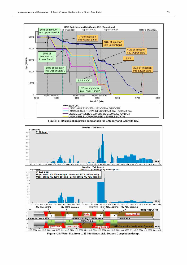
Figure 15: Split design injection rate into the Upper & Lower Sand 1 for I1b. ................................................................ 20 Figure 16: Water flux from well into Sand 1 (Top/Middle: SAS only vs. SAS+ICV). Bottom: Completion design. ...... 21 Figure 17: Schematic of a typical SAS-ICV completion for this case study .................................................................... 21 Figure 18: Annular velocity (v) with zonal isolation in the integrated SAS+ICV completion. The circled (red) shows the

top most screen joint is the weakest point of the completion. .......................................................................................... 21 Figure B-1: The proposed initial selection flowchart and sand control ‘traffic light’ selection output. ........................... 30 Figure B-2: Definition of fines ......................................................................................................................................... 35 Figure D-1: PSD for Sand 2C in Well Dst1 ...................................................................................................................... 38 Figure E-1: Sand 1 (Upper) and Sand 2 (Lower) vertical cross-sections.......................................................................... 40 Figure E-2: Reservoir stimulation shows six wells water injection rates for the first 11 years (Beesley et al. 2011). ..... 41 Figure F-1: Fracture opening pressure of 5450psi (Sand 1D in Reservoir 1). .................................................................. 42 Figure F-2: FMI log of Well D (injectivity test well) through the shale section. ............................................................. 43 Figure F-3: The WSM showing the orientation of σH of the North Sea, UK (courtesy of Helmholtz Centre Potsdam). .. 43 Figure F-4: The location of WIs (including fracture orientations and faults) in seismic and reservoir models. ............... 44 Figure G-1: D50 distribution for Sand 1 ........................................................................................................................... 45 Figure G-2: D10 distribution for Sand 1 ........................................................................................................................... 45 Figure G-3: Sc of Sand 1 .................................................................................................................................................. 46 Figure G-4: Uc vs. depth for Sand 1 ................................................................................................................................. 47 Figure G-5: Formation fines (%) vs. depth for Sand 1 ..................................................................................................... 47 Figure G-6: D50 distribution for Sand 2 ........................................................................................................................... 48 Figure G-7: D10 distribution for Sand 2 ........................................................................................................................... 48 Figure G-8: Sc of Sand 2 .................................................................................................................................................. 49 Figure G-9: Uc vs. depth for Sand 2 ................................................................................................................................. 50 Figure G-10: Formation fines (%) vs. depth for Sand 2 ................................................................................................... 50 Figure H-1: Rock Quality Index (RQI) vs. Sorting (Sc) of Sand 1................................................................................... 53 Figure H-2: Rock Quality Index (RQI) vs. Sorting (Sc) of Sand 2................................................................................... 53 Figure H-3: KV/KH for I1a injector; and for I2 injector (bottom right). ............................................................................ 54 Figure I-1: I1c injection profile comparison for SAS only and SAS with ICV. ............................................................... 58 Figure I-2: Water flux from I1c into Sand 1. Bottom: Completion design. ...................................................................... 59 Figure I-3: I1a injection profile comparison for SAS only and SAS with ICV. ............................................................... 60 Figure I-4: Water flux from I1a into Sand 1. Bottom: Completion design. ...................................................................... 60 Figure I-5: I2b injection profile comparison for SAS only and SAS with ICV. ............................................................... 61 Figure I-6: Water flux from I2b into Sand 2. Bottom: Completion design. ...................................................................... 61 Figure I-7: I2a injection profile comparison for SAS only and SAS with ICV. ............................................................... 62 Figure I-8: Water flux from I2a into Sand 2. Bottom: Completion design. ...................................................................... 62 Figure I-9: I1/ I2 injection profile comparison for SAS only and SAS with ICV. ........................................................... 63 Figure I-10: Water flux from I1/ I2 into Sands 1&2. Bottom: Completion design. .......................................................... 63 Figure I-11: Annular velocity of water injectors in Sand 1. ............................................................................................. 64 Figure I-12: Annular velocity of water injectors in Sand 2. ............................................................................................. 64 Figure I-13: Annular velocity of water injectors in Sands 1 & 2 (commingle). ............................................................... 65 Figure J-1: Visual view used to interpret appraisal cores and wireline logs of the case study. ........................................ 66 Figure K-1: NETool

TM workflow data input..................................................................................................................... 67

Figure K-2: NEToolTM

main menu prior to stimulation. .................................................................................................. 67


LIST OF TABLES

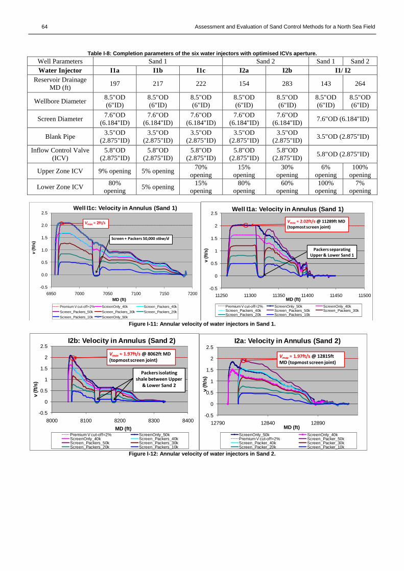
Table B-1: Formation Sand Sorting Values ...................................................................................................................... 28 Table B-2: Proposed Sorting Criteria ............................................................................................................................... 28 Table B-3: Sand Control recommended using Price-Smith et al. methodology ............................................................... 29 Table B-4: Typical CEC values for specific clays ............................................................................................................ 34 Table B-5: Critical flux rates to avoid erosion for various sand control completions ...................................................... 34 Table D-1: Sand Control Selection Table for various types of Standalone Screens (SAS) .............................................. 38 Table D-2: Sand Control Selection Table for Expandable Sand Screens (ESS) ............................................................... 38 Table D-3: Sand Control Selection Table for OHGP-LAWP/ HAWP ............................................................................. 39 Table D-4: Sand Control Selection Table for OHGP-Slurry Pack ................................................................................... 39 Table E-1: Data from appraisal wells used for the case study .......................................................................................... 40 Table E-2: Design injection requirement for the water injectors ...................................................................................... 40 Table F-1: Expected hydraulic fracture orientation of the water injectors ....................................................................... 44 Table G-1: D50 minimum, average and maximum values derived from PSD of Sand 1 DSA ........................................ 45 Table G-2: D10 minimum, average and maximum values derived from PSD of Sand 1 DSA ........................................ 46 Table G-3: Sc (D10/D95) minimum, average and maximum values derived from PSD of Sand 1 DSA ......................... 46 Table G-4: D50 minimum, average and maximum values derived from PSD of Sand 2 DSA ........................................ 48 Table G-5: D10 minimum, average and maximum values derived from PSD of Sand 2 DSA ........................................ 49 Table G-6: Sc (D10/D95) minimum, average and maximum values derived from PSD of Sand 2 DSA ......................... 49 Table G-7: Recommended sand control strategy based on Flowchart B for each unit in Sands 1 and 2 .......................... 51 Table H-1: Shale thickness determination of Sand 1 water injectors based on nearby appraisal logs .............................. 52 Table H-2: Shale thickness determination of Sand 2 water injectors based on nearby appraisal logs .............................. 52 Table H-3: Minimum, average and maximum of intra-shale layer in Shale 2B (coloured) .............................................. 52 Table H-4: R2 values of Sand 1 and Sand 2 ..................................................................................................................... 52 Table I-1: Ratio of kh per unit in Sand 1 for three WIs .................................................................................................... 55 Table I-2: Ratio of kh per unit in a Sand 2 WI (I2a) ......................................................................................................... 55 Table I-3: Ratio of kh per unit in a Sand 2 WI (I2b) ......................................................................................................... 55 Table I-4: Ratio of kh per unit in Sands 1 and 2 for a commingling WI (I1/ I2) .............................................................. 55 Table I-5: A summary of ICV aperture required to achieve the injection split ratios for water injectors in Sand 1 ......... 56 Table I-6: ICV aperture in the commingling I1/ I2 for Sands 1 and 2 .............................................................................. 57 Table I-7: A summary of ICV aperture required to achieve the injection split ratios for water injectors in Sand 2. ........ 58 Table I-8: Completion parameters of the six water injectors with optimised ICVs aperture. ........................................... 64 Table I-9: Sensitivity analysis of annular fluid velocities from 10-50kstbw/d for water injections in both reservoirs. ... 65

Assessment and Evaluation of Sand Control Methods for a North Sea Field A. F. Latiff, Imperial College

R. W. Zimmerman, Imperial College

C. Paveley, Nexen Petroleum UK Ltd.

Abstract It is not uncommon for wells to require sand control, with thousands of them worldwide having been fitted with this

equipment. To do so, service companies and sand control experts have over the years developed a range of guidelines, along

with published and proprietary sand control selection methodologies. Unfortunately, many of the methodologies highlight a

range of design criteria that are specific or complex; resulting in sand control selection being too time-consuming or difficult.

The industry knows that there is no ‘silver bullet’ in choosing a sand control method. Consequently, a study has been

conducted with the purpose of explaining a new sand control selection methodology that is concise and simple to understand.

Furthermore, every sand control method can be assessed and evaluated as long as performance, reliability and cost are safely

and economically justified.

Guiding the engineer to the most appropriate sand control technique, the study consolidates best practice from many

published methodologies, and integrates them with the operator’s sand management guidelines. Consisting of two flowcharts

that end with a sand control equipment, the methodology also supplements each technical choice with a sand control selection

table. This is where risks and concerns are outlined, assuming that the engineer has chosen the sand control resulting from the

flowcharts.

Establishing a sand control selection is required in a North Sea field for its proposed water injectors. The water injectors

are planned for injection under both matrix and fracture regimes into two reservoirs; called here Sand 1 and Sand 2. Sand in

these reservoirs will fail as a result of fracture injection, and the produced sand may backflow into the wellbore once the well

is shut-in. Using the new methodology, openhole premium-type Stand Alone Screen (SAS) is recommended for both

reservoirs. Naturally, the flowchart’s recommendation of premium-type SAS raises concerns, and is outlined in the sand

control selection table. It is found that formation heterogeneity in both Sands 1 and 2 may dampen the performance of the

premium-type SAS injectors. Using the methodology again, the flowchart also suggests the use of blank pipes and packers to

isolate the impermeable shale sections. Inflow control valves are sized and positioned in the completions to counteract the non-

uniform water flux caused by large permeability variation.

Now that a sand control is conceptually selected for the water injectors, the engineer can easily compare the recommended

sand control with other techniques; as part of the overall selection process. Ultimately, this recommendation validates the use

of the new methodology for future sand control selections.

Introduction For over seventy years, the oil and gas industry has continually developed and used sand control completions in reservoirs to

control sand production. This technology has played a pivotal role, and will continue to do so, as well demands are more

challenging and performance expectations are greater. With high operating and well intervention costs, the impact of sand

production cannot be ignored. The effect of formation sand in a well may lead to loss of integrity, and consequently cause the

wellbore to collapse. It is absolutely crucial for the industry to manage sand actively.

Design and selection criteria for sand control methods vary among operators and location. Choice is influenced by local

experience, case studies and service company recommendations. To date, several design methodologies have been published.

For instance, Price-Smith et al. (2003) and Farrow et al. (2004) have published guidelines and selection matrices that have

been widely used by the industry.

The main objective of this paper is to present a simple and easy to understand sand control selection methodology. The

intention is not to reinvent the wheel, but to improve on existing sand control selections. The proposed methodology is built by

consolidating the operator’s sand management guidelines with relevant published papers. Consolidation is then integrated into

a new methodology based on technical experience, laboratory testing and field case studies. The methodology is separated into

two sections – flowcharts, and a ‘traffic light’ design matrix. These flowcharts are subdivided into parts A and B. Flowchart A

is used as a ‘first pass’ selection criterion. It is used to guide the engineer to the most appropriate sand control option.

Flowchart B focuses on the ‘screen and gravel size’ selection, and should be used in conjunction with Flowchart A. Then,

‘traffic light’ design matrix is used as further guidance once a sand control technique has been selected from the flowcharts.

Imperial College London


The ‘traffic light’ concept (ranked by colour) refers to the effectiveness of the selected sand control technique in managing

sand under a variety of wellbore and reservoir conditions. It is important to note that flowcharts and the ‘traffic light’ design

matrix are merely guidelines for the engineer. The engineer is advised to use technical experience, rationality and in-

house/service sand control experts as part of the overall selection process. Further explanation of the new methodology will be

discussed later in this paper.

Study of rock mechanics and sand production prediction are important criteria in determining the most appropriate sand

control. However, due to the limited size imposed on this paper, these topics will only be discussed briefly; focusing on how

and why the sand may fail.

The second objective of this paper is to assess and evaluate suitable sand control methods for water injectors. These water

injectors are part of a Field Development Plan (FDP) and have yet to be completed. The FDP is targeting oil accumulation in

two sandstone reservoirs. Base case development is to drill a number of water injectors with a reservoir trajectory that will give

optimum connectivity between the wellbore and formation. Injection of water into the reservoir will have a design capacity

that is able to accommodate both matrix and formation fracture injection pressures. This is to ensure injectivity is not lost over

time due to formation plugging. Water injection for this field is critical, and has three objectives. Firstly, to dispose produced

water back into the reservoir. Secondly, to optimise sweep efficiency to improve oil recovery; and thirdly to ensure reservoir

pressure is maintained. For wellbore stability, pressure maintenance of the reservoir is important to prevent

compaction/subsidence of the formation and sand production.

Sand control is required to counter sand failure caused by production and operational issues. These issues can lead to

several failure mechanisms. The failure mechanisms are water hammer, well backflow, reservoir cross flow and erosion

(Santarelli et al., 2000). These effects, if not accounted for, will cause a significant drop in injectivity over time. Inflow control

technology will be modelled using NEToolTM

as part of the selection to ensure uniform injectivity across all intervals.

In this case study, the sand control equipment is selected based on the outcome of flowcharts A and B. The ‘traffic light’

design matrix is then used to highlight the concerns and risks associated with the chosen sand control method. As long as the

concerns and risks are accounted for, recommending the sand control based on the methodology can easily be justified. The

outcome of this new methodology is an attempt to improve the selection consistency across the industry.

Methodology: Sand Control Selection The proposed methodology for sand control concept selection using flowcharts is illustrated in Figures 1 and 2. The

workflow in these illustrations focuses more on sand control for openhole completions. Sand control for cased hole completion

is also outlined in Flowchart A. The flowcharts are supplemented by a sand control selection table highlighting risks and

concerns of each technique-presented in Table D-1 to D-4 in Appendix D.

Flowchart A – ‘First Pass’ Selection Criteria

Flowchart A is an identification process to guide the engineer to the most appropriate sand control option. The start of this

flowchart assumes that sand production will occur and sand control is required. The decision for an openhole or cased hole

completion depends on rock geomechanics, wellbore stability and reservoir strategy. An openhole completion is favoured

where high production rates are required and if the formation intervals are allowed to commingle. It is not a recommended

completion if wellbore stability is poor and a large amount of fine sand is present. Fines are produced from the formation

matrix as a result of increased stress and fluid movement. Cased hole completion is an alternative to openhole. It gives stability

to wellbore integrity and provides isolation for productive intervals from unwanted gas and water. Most importantly, cased

hole completion allows selective and oriented perforating that can delay or eliminate sand production.

Assuming openhole completion is defined, the next design criterion is the sand size analysis. This analysis is based on the

methodology proposed by Tiffin et al. (1998). The study is used as a screening process in Flowchart A and further evaluated in

Flowchart B. For example, if the formation has uniformity coefficients (D40/D90) of <5, D10 grain sizes >175μm, and mobile

fines of less than 5%, the methodology recommends Standalone Screen (SAS) or Expandable Sand Screen (ESS).

After the study of sand size analysis, the presence and condition of shale in the formation must be studied. If a large slab of

shale (greater than 30 ft) is present and unstable, it will require isolation. To achieve this, openhole packers and blank pipes are

used across these sections. This is to prevent weakened shale from producing fines that can be detrimental to the sand control.

Additionally, openhole packers can reduce annular flow and shut-off unwanted water or gas formations.

A large variation in reservoir permeability will require the use of inflow control technology in conjunction with sand

control. Inflow Control Devices (ICD) or Inflow Control Valves (ICV) can control the amount of liquid flow and provide a

more uniform distribution profile between the wellbore and reservoir zones. Controlling the flow will also reduce the annular

flow velocity, preventing the formation of ‘hot spots’ that is a concern for sand control screen. The use of ICD is more

applicable for horizontal wells to counteract the ‘heel-to-toe’ effect (Khalil et al. 2010). The ‘heel-to-toe’ effect causes a higher

influx of liquid at the heel of the horizontal completion. To summarise, not accounting for permeability heterogeneity in the

selection process may lead to water or gas breakthrough at an early stage of recovery.

ESS is recommended for reservoirs with similar permeability or when zonal isolation is not required. The advantage of

using ESS is that it provides a larger inflow area and reduces pressure loss across the completion. It also eliminates annular

flow between the screen annulus and wellbore. However, ESS is not recommended if the formation contains reactive shale.


Unstable shale can lead to breakouts or clay swelling, thus complicating its installation and use. This is because ESS has lower

material strength than a conventional SAS.

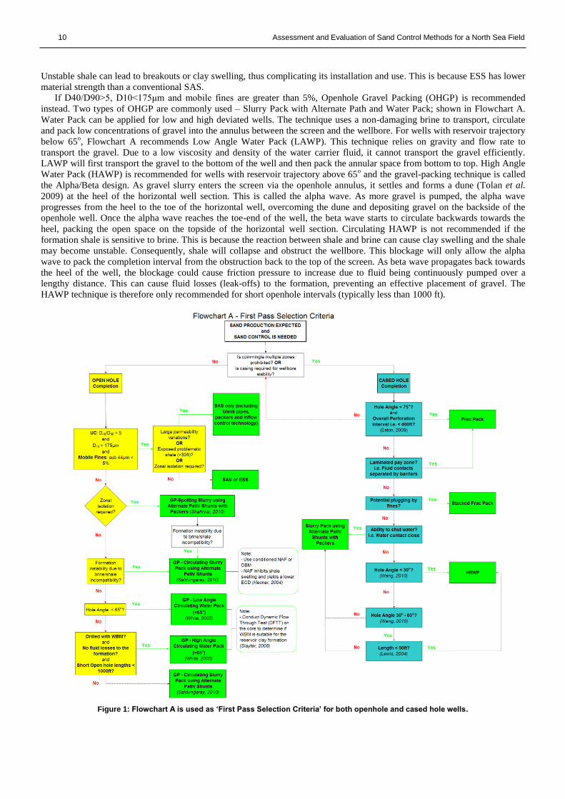
If D40/D90>5, D10<175μm and mobile fines are greater than 5%, Openhole Gravel Packing (OHGP) is recommended

instead. Two types of OHGP are commonly used – Slurry Pack with Alternate Path and Water Pack; shown in Flowchart A.

Water Pack can be applied for low and high deviated wells. The technique uses a non-damaging brine to transport, circulate

and pack low concentrations of gravel into the annulus between the screen and the wellbore. For wells with reservoir trajectory

below 65o, Flowchart A recommends Low Angle Water Pack (LAWP). This technique relies on gravity and flow rate to

transport the gravel. Due to a low viscosity and density of the water carrier fluid, it cannot transport the gravel efficiently.

LAWP will first transport the gravel to the bottom of the well and then pack the annular space from bottom to top. High Angle

Water Pack (HAWP) is recommended for wells with reservoir trajectory above 65o and the gravel-packing technique is called

the Alpha/Beta design. As gravel slurry enters the screen via the openhole annulus, it settles and forms a dune (Tolan et al.

2009) at the heel of the horizontal well section. This is called the alpha wave. As more gravel is pumped, the alpha wave

progresses from the heel to the toe of the horizontal well, overcoming the dune and depositing gravel on the backside of the

openhole well. Once the alpha wave reaches the toe-end of the well, the beta wave starts to circulate backwards towards the

heel, packing the open space on the topside of the horizontal well section. Circulating HAWP is not recommended if the

formation shale is sensitive to brine. This is because the reaction between shale and brine can cause clay swelling and the shale

may become unstable. Consequently, shale will collapse and obstruct the wellbore. This blockage will only allow the alpha

wave to pack the completion interval from the obstruction back to the top of the screen. As beta wave propagates back towards

the heel of the well, the blockage could cause friction pressure to increase due to fluid being continuously pumped over a

lengthy distance. This can cause fluid losses (leak-offs) to the formation, preventing an effective placement of gravel. The

HAWP technique is therefore only recommended for short openhole intervals (typically less than 1000 ft).

Figure 1: Flowchart A is used as ‘First Pass Selection Criteria’ for both openhole and cased hole wells.


Slurry Pack is another OHGP technique that uses a more viscous carrier fluid than the carrier fluid used for water pack. It

stabilises the formation while ensuring well productivity is not compromised. The technique is suitable for formations with

brine-sensitive shale, low fracture gradients (i.e. high fluid losses) and large variations in permeability. In other words, it is

suitable for well conditions when LAWP or HAWP are not recommended. Slurry pack uses alternate path or nozzle-type shunt

tubes to circulate the slurry down the openhole via the screen annulus; packing it from the toe and back to the heel of the

horizontal well section. When a bridge forms in the annulus as a result of high leak-offs, the annulus packs only from the

formed bridge back to the top of the screen. As the sand covers the top of the screen, diverting the slurry via the shunt tubes

instead creates sufficient pressure. The slurry exits the shunt tubes below the formed bridge and packs any remaining voids in

the screen annulus. Circulating slurry is recommended for long openhole intervals (>1000 ft).

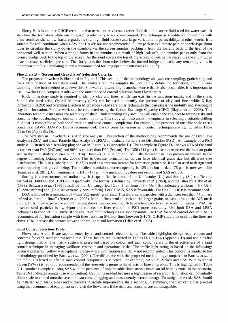
Flowchart B – ‘Screen and Gravel Size’ Selection Criteria.

The proposed flowchart is illustrated in Figure 2. This section of the methodology analyses the sampling, grain sizing and

fines identification of formation sand. The analysis requires samples that accurately define the formation, and full core

sampling is the best method to achieve this. Sidewall core sampling is another source that is also acceptable. It is important to

use Flowchart B to compare results with the outcome sand control selection from Flowchart A.

Rock mineralogy study is required to identify clay and fines, which can exist in the sandstone matrix and in the shale.

Should the need arise, Optical Microscopy (OM) can be used to identify the presence of clay and fines while X-Ray

Diffraction (XRD) and Scanning Electron Microscope (SEM) are other techniques that can assess the mobility and swelling of

clay in a formation. Further work can be conducted using the Cation Exchange Capacity (CEC) (Slayter et al. 2008). This

laboratory technique measures the reactivity of shale. Understanding clay swelling will enable the engineer to foresee risks and

concerns when evaluating various sand control options. This study will also assist the engineer in selecting a suitable drilling

mud that is compatible to both the formation and sand control completion. For example, the presence of unstable shale raises

concerns if LAWP/HAWP or ESS is recommended. The concerns for various sand control techniques are highlighted in Table

D1 to D4 (Appendix D).

The next step in Flowchart B is sand size analysis. This section of the methodology recommends the use of Dry Sieve

Analysis (DSA) and Laser Particle Size Analysis (LPSA) to evaluate Particle Size Distribution (PSD). An example of a PSD

study is illustrated on a semi-log plot; shown in Figure D-1 (Appendix D). The example in Figure D-1 shows 40% of the sand

is coarser than D40 (247 m) and 90% is coarser than D90 (94 m). The D50 (214 m) is used to represent the median grain

size in the PSD study (Saucier et al. 1974). However, D50 is not applied in the flowchart as it is proven insensitive to the

degree of sorting (Xiang et al., 2003). This is because formation sands can have identical grain size but different size

distributions. The D10 (Coberly et al. 1937) is used as a criterion instead for formation grain size. It is also used to design sand

screen opening and gravel sizing. The smallest standalone screen opening is 125 m but to date, 75 m is now available

(Franklin et al. 2011). Conventionally, if D10 <175 m, the methodology does not recommend SAS or ESS.

Sorting is a measurement of uniformity. It is quantified in terms of the Uniformity (Uc) and Sorting (Sc) coefficients

defined as D40/D90 and D10/D95, respectively. The former is defined by Schwartz et al. (1969), and the latter by Tiffin et al.

(1998). Schwartz et al. (1969) classified four Uc categories: [Uc < 3: uniform], [3 < Uc < 5: moderately uniform], [5 < Uc <

10: non-uniform] and [Uc > 10: extremely non-uniform]. For 0<Uc<5, SAS is favourable. For Uc>5, OHGP is recommended.

DSA is limited to a minimum of 44μm (325-mesh) grain size. Therefore, sand particles with a diameter less than 44 μm are

defined as “mobile fines” (Byrne et al. 2008). Mobile fines tend to stick to the larger grains or pass through the 325-mesh

during DSA. Field experience and lab testing shows fines exceeding 5% have a tendency to cause screen plugging. LPSA can

measure sand particles below 44μm and reflects the finer end of the PSD more accurately. Use both DSA and LPSA

techniques to conduct PSD study. If the results of both techniques are incomparable, use DSA for sand control design. SAS is

recommended for formation sample with fines less than 5%. For fines between 5-10%, OHGP should be used. If the fines are

above 10%, increase the contact between the wellbore and formation (Tiffin et al. 1998).

Sand Control Selection Table.

Flowcharts A and B are supplemented by a sand control selection table. The table highlights design requirements and

concerns for each sand control technique. These factors are illustrated in Tables D-1 to D-4 (Appendix D) and use a traffic

light design matrix. The matrix system is presented based on colour and each colour refers to the effectiveness of a sand

control technique in managing wellbore, reservoir and operational risks. The traffic light rating is based on the following:

Green = preferred, yellow = acceptable, orange = use with caution and red = not recommended. This concept is similar to the

methodology published by Farrow et al. (2004). The difference with the proposed methodology compared to Farrow et al. is

the table is referred to after a sand control equipment is selected. For example, SAS Pre-Packed and SAS Wire Wrapped

Screen (WWS) is red (not recommended) if the reservoir is prone to the effects of fines migration. This is highlighted in Table

D-1. Another example is using SAS with the presence of impermeable shale streaks inside an oil bearing zone. In this scenario,

Table D-1 indicates orange (use with caution). Caution is needed because a high degree of reservoir lamination can potentially

allow shale to embed onto the screen. It can cause plugging and consequently screen damage. To mitigate the risk, SAS should

be installed with blank pipes and/or packers to isolate impermeable shale sections. In summary, the user can either proceed

using the recommended equipment or re-visit the flowcharts if the risks and concerns are unmanageable.


A range of sand control options has been documented in the methodology. Below are some sand control options (illustrated

in Flowcharts A and B) that will be assessed and evaluated for a case study; discussed in the next section:

- Openhole Standalone Screen (OHSAS)

o Wire-wrapped, Pre-packed and Premium

- Expandable Sand Screen (ESS)

- Openhole Gravel Pack (OHGP)

o Low Angle Circulating Water Pack

o High Angle Circulating Water Pack (Alpha/Beta Design)

o Slurry Pack with Alternate Path/ Shunt Tubes

Flowchart B - Screen and Gravel Size Selection

Type & Behaviour of

Clay

CEC

meq/100g)

Swelling Smectites 80-150

Mobile Kaolinites 1-10

(Slayter et al. 2008)

Flowchart B Glossary

APT Alternate Path Technology

CEC Cation Exchange Capacity

DIF Drill-In Fluid

DSA Dry Sieve Analysis

ESS Expandable Sand Screen

GP Gravel Pack

LPSA Laser Particle Size Analysis

OM Optical Microscopy

SAS Standalone Screen

SEM Scanning Electron Microscope

SRT Sand Retention Test

XRD X-Ray Diffraction

Not Recommended

Use With Caution

Acceptable

Preferred

Sand Size Analysis

Formation Grain Size for Sizing

D10 < 175μm?

Uniformity Coeff.: (D40/D90)

Uc> 5?

Sorting Coeff.D10/D95 < 10?

No

Uniformity Coeff.

(D40/D90) (Uc)

Yes

CEC analysis

XRD/ SEM Analysis

Swelling clays?

No

Fines < 2%?Yes

2< Fines<5%?

Fines > 10%

Increase contact between well and

formation(Tiffin et al. 1998)

OM AnalysisClay present in sandstone

matrix?Clay present inside shale?

No

DSA

Note on XRD/ SEM:- Identifies cementation and fines.

- Identifies clay and fines. Clay swelling can cause problems during sand control installation

(Napalowski, 2010) and will dictate the type of DIF used.- To determine whether GP water pack will be

suitable for the formation

SAS only

GP-Slurry pack using APT

GP-Water Pack (Alpha/Beta design)

ESS

GP-Slurry pack using APT

GP-Water Pack (Alpha/Beta design)

Yes

Yes

Yes

Conduct SRT

LPSA

Same results

DSA/ LPSA

combined

NoYes

DSA only

Uc < 3?

3 < Uc < 5?

No

Yes

Yes

5< Fines<10%?

No

No

SAS-Wire Wrapped

SAS-Premium/ Mesh

Yes

Measures shale reactivity(i.e. CEC > 20: Highly reactive)

(McKay et al. 2000)

FORMATION SAND ANALYSIS

No

Yes

Conduct SRT

No

Uc > 5

No

Yes

No

Figure 2: Flowchart B represents ‘Screen and Gravel Size Selection’.


Results: Verification of Methodology

Case Study – North Sea Field, UK

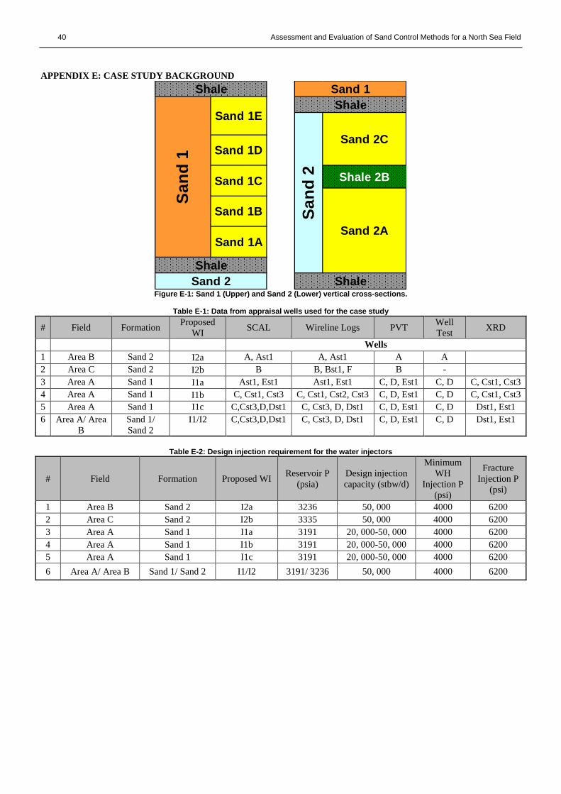
Background. The North Sea field was initially discovered in 2006. It lies in the UK sector of the North Sea at a water depth of

370 ft. There are two turbidite reservoirs of interest located in two sandstone reservoirs. For this case study, these reservoirs

are called Sand 1 and Sand 2 – the former is divided into five zones and the latter divided into three zones. Figure E-1 in

Appendix E shows the vertical subdivision of the reservoirs. Sand 2 has some support from an aquifer but Sand 1 has little

natural pressure support. Both reservoirs are separated by shale, and it is uncertain whether or not Sands 1 and 2 are in

communication.

Sand 1 is highly heterogeneous. It contains thinly bedded sand and shale streaks (1-2 ft) embedded inside the sandstone

matrix. The porosity ranges between 14-20%, permeability in the order of 0.2–0.7 D, and net-to-gross between 33-83%. On the

other hand, Sand 2 is more homogeneous with little shale content. It consists of clean quality sandstone with a thick intra-

bedded shale formation (15-20 ft) separating the upper and lower zones. It has porosity in the range of 18-24% and

permeability in the order of 0.7-1.4 D.

Available data is obtained from several appraisal wells (Table E-1). Study of the appraisal cores and wireline logs shows

sand failure will occur and sand control is required when completing these wells.

Injection Strategy. The overall objectives of the water injectors are to dispose produced water back into the reservoir, optimise

sweep efficiency to improve oil recovery and provide reservoir pressure maintenance. Initially, the water will be injected under

the matrix regime. Over time, injectivity losses may occur as a result of the failed sand plugging the formation. To mitigate

this, the design of water injectors will have the capacity to maintain and increase injection pressures to levels resulting in

formation fracturing. Therefore, this requires a well trajectory that will give the maximum connectivity between the wellbore

and formation. To achieve this, the orientation of the in-situ stress for the field must be determined in order to predict the

orientation of the induced fractures. Cold Low Sulphate Seawater (LSSW) and produced formation water will be used as the

injection fluids. This will enhance the creation of induced fractures by thermally reducing the fracture pressure (Perkins and

Gonzales et al. 1984, Svendsen et al. 1991).

The design capacity of the water injectors is shown in Table E-2. The water injectors will be drilled in the oil and water leg

of Sands 1 and 2 respectively. One out of the six water injectors will commingle and provide injection support into both

reservoirs. The initial reservoir pressure (Pi) for both reservoirs varies from 3191 to 3335 psia. Stimulation shows with water

injection support, the maximum depletion (∆P) for both reservoirs are expected to drop between 400-500 psia, which is still

above the bubble point pressure (Pb). To achieve this, stimulation shows the injections are required from 10, 000 to 28, 000

stbw/d for Sand 1 and 14, 000 to 35, 000 stbw/d for Sand 2.

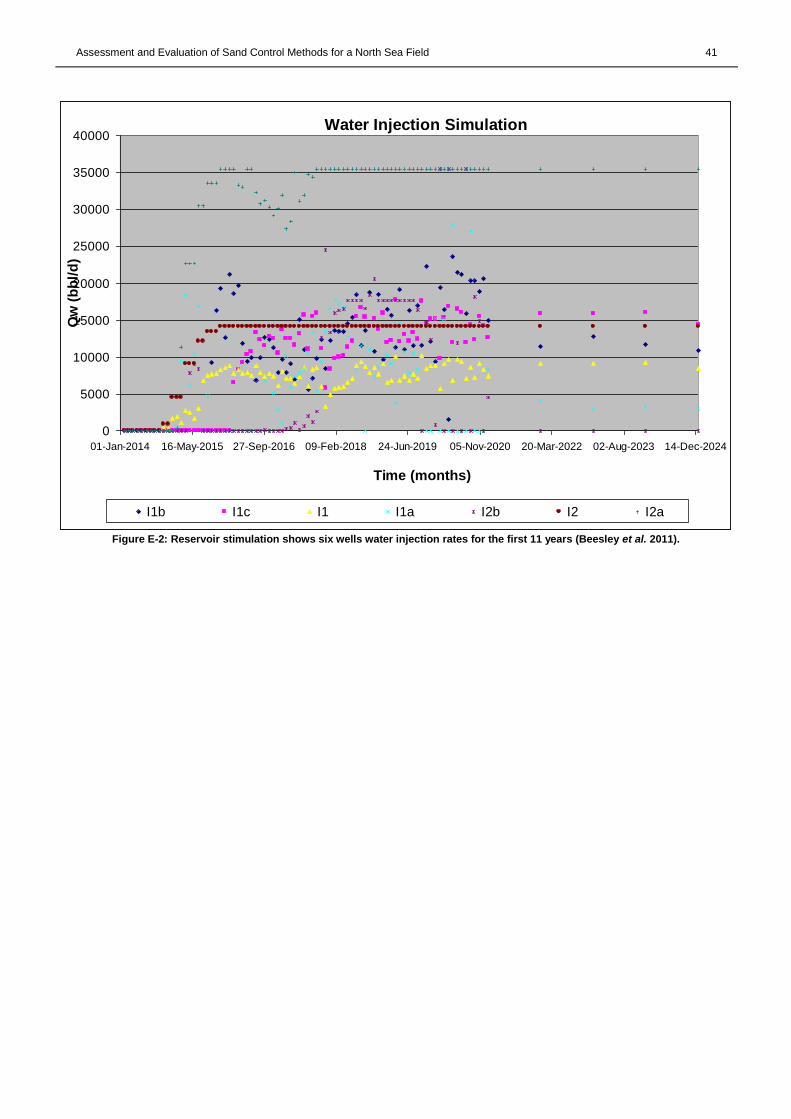
The design of the water injectors will have the capacity to accommodate injection rates in the range of 40, 000 to 50, 000

stbw/d. Figure E-2 shows the reservoir simulation of the water injectors for the first 11 years. The water injectors labelled I1

and I2 represent wells in Sands 1 and 2, respectively. Well I1/I2 means the water injector injects into both reservoirs.

Rock Mechanics and In-Situ Stresses.

The load on a rock depends on in-situ stresses, reservoir pressure and drawdown. Understanding the evolution of formation

in-situ stresses is an important step in rock mechanics. Sources of these stresses are vertical (σv), horizontal maximum (σH) and

horizontal minimum (σh). The magnitude and orientation of these stresses are critical parameters especially when injecting

water in the fracture regime. The wellbore should be accurately oriented along an azimuth parallel to σH (White et al. 2011). A

good connectivity between the wellbore and formation fractures will optimise injectivity into the reservoir.

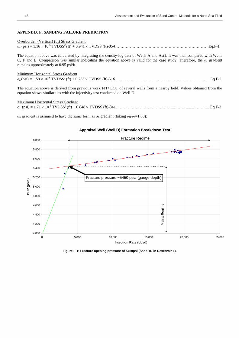
For this case study, σv is approximated by a gradient of 0.97 psi/ft using Equation F-1 in Appendix F. The σv reflects the

weight of the earth above the depth of interest. The σh stress gradient is approximated at 0.75 psi/ft using Equation F-2 (below).

The equation was determined from previous Leak-Off Tests (LOT) and Formation Integrity Tests (FIT). Applying Equation F-

2, σh=5378 psi at 7150 ft TVDSS. The σh is similar to the outcome of injectivity test from a nearby appraisal well (Well D),

where the fracture opening pressure (Pfrac) was 5450 psia (Figure F-1 in Appendix F). The similarity proves σh gradient is valid

for this case study.

The magnitude of σH is difficult to calculate. In most cases, all of the in-situ stresses are not required as the σv and σh are

the key parameters in predicting sand production. Using North Sea anisotropy (σH/σh) of 1.08, σH can be calculated. Here, σv

(0.97 psi/ft) is larger than σH and σh (0.81 psi/ft and 0.75 psi/ft) (σv>σH>σh). This is common but may not true be for active-

tectonic areas; where σv can be the intermediate or smallest stress.

The orientation of σh can be determined from caliper or by examining drilling-induced fractures using Formation Image

(FMI) logs. Figure 3 below shows there is no evidence of borehole breakouts or drilling-induced fractures in both the caliper

and FMI logs. Figure F-2 in Appendix F shows the same result through a shale section in Well D.


Figure 3: Section of Well Est1 wireline log from 9330 to 9440ft MD (Reservoir 1). The Formation Image (FMI) and caliper logs show no

evidence of borehole breakouts and washouts respectively.

Absence of borehole breakouts in the appraisal wells suggests that σH and σh may have little anisotropy in the horizontal

plane (σV>σH~σh). A geomechanical study from a nearby field show that σH and σh have magnitudes similar to each other (i.e.

almost isotropic) (Persaud et al. 2009).

The uncertainty in determining the in-situ stresses orientations remains large. The World Stress Map (WSM) is a useful

starting point to reduce this uncertainty. Figure F-3 shows a schematic of the North Sea regional stresses, revealing that σH has

a generalised NNW-SSE trend. However, the scale of the North Sea regional stress may be erroneous because the local stress

orientation varies from one fault block to another (Yale et al. 1994). The regional trend from WSM, however, is fairly

consistent with the local stress regimes of two nearby fields; where σH direction is 095 o to 275

o (±20

o) (almost W-E trend).

Existing faults in the reservoir will give a clue of σH and σh orientations. Induced fractures tend to orient themselves in the

same direction as the existing faults or along the azimuth of σH direction (Gorden et al. 2011). This assumption is not valid if

the horizontal stress regime of the reservoir has changed between the time the faults were created and now, which is unlikely.

Figure F-4 and Table F-1 in Appendix 4 shows the location and the expected fracture orientation of the water injectors. The

uncertainties in σH/σh anisotropy limit the deviations of injectors to less than 30o (near vertical) across the reservoir interval.

This is to ensure efficient fracture connectivity is achieved regardless of the orientation of σH.

Particle Size Distribution (PSD).

Core data from the appraisal wells are available for study. These data were used to determine the D10 formation grain size,

Sc, Uc and fines. DSA and LPSA techniques are used in combination to ensure the fines portions are accurately quantified.

Figures 4 and 5 shows there are large differences of fines portion in Sands 1 and 2 when comparing DSA and LPSA

techniques. The large difference is expected because DSA measures larger fines (>44 μm) and LPSA is more accurate for

measuring fines below 44 μm. Fines with grain sizes below 44 μm tend to disappear as ‘dust’ and also adhere to coarser

particles during sieving (Slayter et al., 2008). LPSA is therefore used to represent the finer end of the particles in Sands 1 and

2. PSD for Sands 1 and 2 are shown in Figure 6 and Figure 7 respectively.

Sand 1: Comparison of Dry Sieve Analysis (DSA) and Laser

Particle Size Analysis (LPSA)

6800

6850

6900

6950

7000

7050

7100

0 10 20 30 40 50 60

Uniformity Coefficient (Uc) (D40/D90)

Depth

(ft

MD

)

Well C-DSA Well C-LPSA

Sand 1: Comparison of Dry Sieve Analysis (DSA) and Laser Particle

Size Analysis (LPSA)

0

5

10

15

20

25

30

0 5 10 15 20 25 30Uniformity Coefficient (Uc) (D40/D90)

Fin

es s

ub

44μ

m (

%)

Well C-DSA Well C-LPSA Well Est1-DSA Well Est1-LPSA

Figure 4: Large variation in fines for Sand 1 show LPSA gives accurate measurement of fines below 44μm.



Particle Size Analysis (LPSA

9500

9520

9540

9560

9580

9600

9620

9640

9660

9680

0 2 4 6 8 10 12 14 16Uniformity Coefficient (Uc) (D40/D90)

Depth

(ft

MD

)

Well Ast1-DSA Well Ast1-LPSA


Particle Size Analysis (LPSA)

0

5

10

15

20

25

30

0 5 10 15 20 25 30Uniformity Coefficient (Uc) (D40/D90)

Fin

es s

ub

44μ

m (

%)

Well Ast1-DSA Well Ast1-LPSA Well Dst1DSA Well Dst1-LPSA

Figure 5: Large variation in fines for Sand 2 show LPSA gives accurate measurement of fines below 44μm.

D50D50

D90D90

D10D10

0

10

20

30

40

50

60

70

80

90

100

110100100010000

Cu

mu

lati

ve

wt%

Grain Size (microns)

Sand 1 Dry Sieve PSD

D10=175μm

Fines are characterised using LPSA

Figure 6: Particle Size Distribution (PSD) of Sand 1 using DSA and LPSA combined (Beesley et al. 2011).

D50D50

D10D10

D90D90

D10=175μm

0

10

20

30

40

50

60

70

80

90

100

110100100010000

Cu

mu

lati

ve w

t%


Sand 2 Dry Sieve PSDFines are characterised

using LPSA

Figure 7: Particle Size Distribution (PSD) of Sand 2 using DSA and LPSA combined (Beesley et al. 2011).


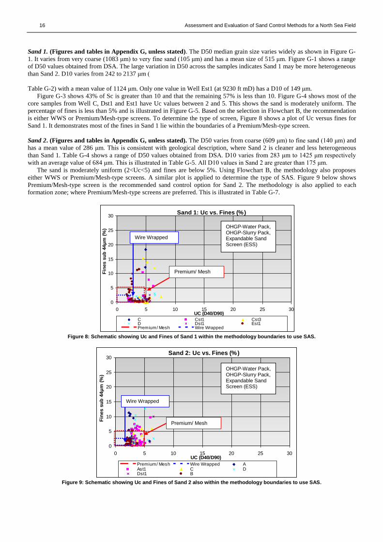
Sand 1. (Figures and tables in Appendix G, unless stated). The D50 median grain size varies widely as shown in Figure G-

1. It varies from very coarse (1083 μm) to very fine sand (105 μm) and has a mean size of 515 μm. Figure G-1 shows a range

of D50 values obtained from DSA. The large variation in D50 across the samples indicates Sand 1 may be more heterogeneous

than Sand 2. D10 varies from 242 to 2137 μm (

Table G-2) with a mean value of 1124 μm. Only one value in Well Est1 (at 9230 ft mD) has a D10 of 149 μm.

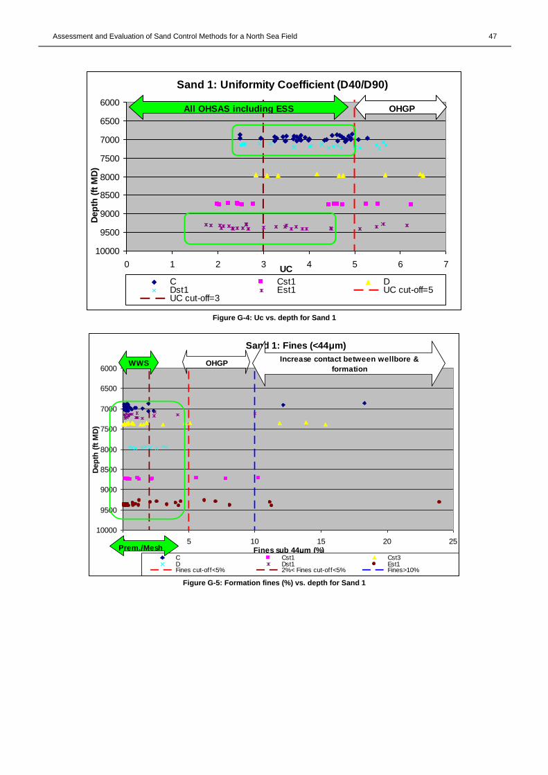
Figure G-3 shows 43% of Sc is greater than 10 and that the remaining 57% is less than 10. Figure G-4 shows most of the

core samples from Well C, Dst1 and Est1 have Uc values between 2 and 5. This shows the sand is moderately uniform. The

percentage of fines is less than 5% and is illustrated in Figure G-5. Based on the selection in Flowchart B, the recommendation

is either WWS or Premium/Mesh-type screens. To determine the type of screen, Figure 8 shows a plot of Uc versus fines for

Sand 1. It demonstrates most of the fines in Sand 1 lie within the boundaries of a Premium/Mesh-type screen.

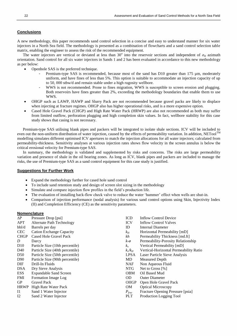
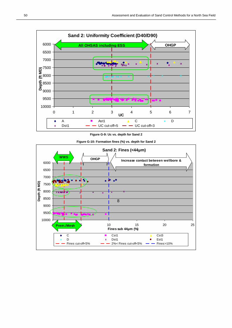
Sand 2. (Figures and tables in Appendix G, unless stated). The D50 varies from coarse (609 μm) to fine sand (140 μm) and

has a mean value of 286 μm. This is consistent with geological description, where Sand 2 is cleaner and less heterogeneous

than Sand 1. Table G-4 shows a range of D50 values obtained from DSA. D10 varies from 283 μm to 1425 μm respectively

with an average value of 684 μm. This is illustrated in Table G-5. All D10 values in Sand 2 are greater than 175 μm.

The sand is moderately uniform (2<Uc<5) and fines are below 5%. Using Flowchart B, the methodology also proposes

either WWS or Premium/Mesh-type screens. A similar plot is applied to determine the type of SAS. Figure 9 below shows

Premium/Mesh-type screen is the recommended sand control option for Sand 2. The methodology is also applied to each

formation zone; where Premium/Mesh-type screens are preferred. This is illustrated in Table G-7.

Sand 1: Uc vs. Fines (%)

0

5

10

15

20

25

30

0 5 10 15 20 25 30UC (D40/D90)

Fin

es s

ub

44μ

m (

%)

C Cst1 Cst3D Dst1 Est1Premium/ Mesh Wire Wrapped

Figure 8: Schematic showing Uc and Fines of Sand 1 within the methodology boundaries to use SAS.

Sand 2: Uc vs. Fines (%)

0

5

10

15

20

25

30

0 5 10 15 20 25 30UC (D40/D90)

Fin

es s

ub

44

μm

(%

)

Premium/ Mesh Wire Wrapped AAst1 C DDst1 B

Figure 9: Schematic showing Uc and Fines of Sand 2 also within the methodology boundaries to use SAS.

Premium/ Mesh

Wire Wrapped

OHGP-Water Pack, OHGP-Slurry Pack, Expandable Sand Screen (ESS)

OHGP-Water Pack, OHGP-Slurry Pack, Expandable Sand Screen (ESS)

Premium/ Mesh

Wire Wrapped


Formation Heterogeneity.

Shale and Zonal Isolation. Openhole completions provide the greatest opportunity to maximise reservoir flow potential.

However, the presence and condition of shale in a productive formation must be investigated, as it may prove problematic.

Earlier PSD studies suggest OHSAS is favoured sand control option. This means that the mineralogy study of shale is not

essential; it is more useful for OHGP. Mineralogy study of clay swelling helps to determine the compatibility of the gravel

pack carrier fluid to shale. If the study shows clay swelling is not critical, a less costly gravel pack carrier fluid can be used

over a more sophisticated and expensive option such as lower-viscosity carrier fluid. A significant cost saving can therefore be

achieved.

The uppermost zone in Sand 1 (i.e. Sand 1E) is more heterogeneous than the lower zones. Across Sand 1, all five zones

contain thin beds of sand and shale with thicknesses of less than 2 ft. Zonal isolation in Sand 1 is difficult. It is also

unfavourable to isolate thin shale sections; risking isolating potential pay zones as well. The uncertainty of isolating shale in

Sand 1 will be reduced after a well is drilled and logged. For estimation purposes, the thickness of shale layers in the reservoir

is determined from the case study appraisal wells. The thickness of shale layers in Sands 1 and 2 are based on shale cut-offs

(Vsh) of 0.4 and 0.5. This is illustrated in Table H-1 and Table H-2. Using Vsh cut-offs of 0.4 and 0.5, it calculates an average

and maximum shale thickness of 6 ft and 25 ft respectively. These values are then used to estimate the length of blank pipes

and packers.

Sand 2 consists of three zones – Sand 2A, Shale 2B and Sand 2C. Sands 2A and 2C are fairly homogeneous and considered

excellent quality sand. It contains low siltstone and mudstone content. Shale 2B is an impermeable zone; separating Sand 2A

from Sand 2C. Its thickness varies from 2-36 ft laterally across the reservoir with an average thickness of 11 ft (Table H-3).

Flowchart A recommends isolation of shale intervals with thicknesses greater than 30 ft by using a combination of blank pipes

and packers.

Permeability Variation. The permeability (k) of Sand 1 varies from 0.2 to 0.7 D and Sand 2 from 0.7 to 1.4 D. Figure 10 and

Figure 11 illustrates permeability-porosity (k-) relationship with porosity cut-offs for Sand 1 and Sand 2 respectively. The left

plot on Figure 10 shows Sand 1 has a wider k- distribution and lower R2

values compared to Sand 2 (Figure 11). This is

another indication that Sand 2 is cleaner and less heterogeneous than Sand 1.

The R2 values are obtained by applying a best fit regression of the k- relationship. The higher the R

2, the less

heterogeneous the formation is. Table H-4 in Appendix H summarised the regressed R2 values for all the appraisal wells. The

average R2 values are therefore 0.78 and 0.83 for Sand 1 and Sand 2 respectively. However, the R

2 needs to be verified because

the value is also dependant on sorting. This is conducted by plotting the Rock Quality Index (RQI) versus Sc. This is illustrated

in Figure H-1 and Figure H-2 for Sands 1 and 2 respectively. Figure H-1 shows a wider RQI and Sc distribution (i.e. less

sorted) compared to Figure H-2. In short, this concludes that a more sorted formation is less heterogeneous (Sand 2) and a less

sorted formation is more heterogeneous (Sand 1); validating the use of R2 to represent heterogeneity in this study.

Sand 1 - K H vs. POR H

R2 = 0.7968

R2 = 0.9134

R2 = 0.6403

R2 = 0.7352

R2 = 0.8289

R2 = 0.7799

0.01

0.1

1

10

100

1000

10000

0 5 10 15 20 25 30 35Ø H (%)

KH

(m

D)

C Cst1 Cst3 D Dst1 Est1 Porosity cut-off 12%

Sand 1 - K V vs. POR V

0.01

0.1

1

10

100

1000

10000

0 5 10 15 20 25 30 35Porosity (%)

KV

(m

D)

Cst1 Cst3 Dst1 Est1 Porosity cut-off 12%

Figure 10: Permeability and porosity relationship of Sand 1 in the horizontal and vertical direction.


Sand 2 - K H vs. POR H

R2 = 0.8157

R2 = 0.7282

R2 = 0.8848

R2 = 0.9207

R2 = 0.819

R2 = 0.7861

0.01

0.1

1

10

100

1000

10000

0 5 10 15 20 25 30 35Ø H (%)

KH

(m

D)

A Ast1 B C D Dst1 Porosity cut-off 13%

Sand 2 - K V vs. POR V

0.01

0.1

1

10

100

1000

10000

0 5 10 15 20 25 30 35Porosity (%)

KV

(m

D)

B C Dst1 Porosity cut-off 13%

Figure 11: Permeability and porosity relationship of Sand 2 in the horizontal and vertical direction.

Uncertainty in determining permeability variation in a pre-drilled injector is large. However, study of nearby appraisal

wells suggests there is a large variation in permeability; especially in Sand 1. Figure 12 shows Sand 1 has anisotropic vertical

(kV) and horizontal (kH) permeabilities, with a vertical-horizontal permeability ratio (kV/kH) ranging from 0.001 to 100.

Following that, Figure 13 shows Sand 2 is less anisotropic compared to Sand 1. More kV/kH plots for Sands 1 and 2 are

illustrated in Figure H-3 in Appendix H. Flowchart A recommends the use of blank pipes, packers and inflow control

technology to counteract the effects of permeability variation in Sands 1 and 2. Large permeability variation can result in

several aforementioned failure mechanisms that are common in water injectors.

Split Injection Rate and Annular Flow

As the need for inflow control technology to be integrated with SAS has been established, a study on how to design and

optimise this integrated completion is required. Inflow-control technology will help to optimise sweep efficiency in highly

heterogeneous Sand 1 and provide pressure support in Sand 2. It will also help to avoid formation fractures in the high

permeability zones by controlling the amount of water intake. ‘Active’ ICV and ‘Passive’ ICD (Birchenko et al. 2008) helps to

improve equalisation and distribution of water evenly across each pay zone. The base design is to position one ICV combined

with openhole packers per zone. ICV is preferred because it is surface-controlled and does not require well intervention. ICD

however is more suited to counteract the ‘heel-to-toe’ effect seen in horizontal wells (Birchenko et al. 2008).

Sand 1: KV/KH (Well Dst1) (for I1 & I1C)

7000

7050

7100

7150

7200

7250

7300

0.0001 0.001 0.01 0.1 1 10 100 1000 10000

KV/KH

De

pth

(ft

MD

)

Dst1 Top of Sand 1E Top of Sand 1C Top of Shale KV/KH Isotropic

Sand 1 - KV/KH (Well Est1) (for I1a)

9200

9250

9300

9350

9400

9450

9500

9550

0.0001 0.001 0.01 0.1 1 10 100 1000KV/KH

De

pth

(ft

MD

)

Est1 Top of Sand 1E Top of Sand 1C Top of Shale KV/KH Isotropic

Figure 12: Vertical-to-horizontal permeability ratio (KV/KH) in Sand 1 is more anisotropic than Sand 2.


Sand 2: KV/KH (Well B) (for I2b)

7500

7550

7600

7650

7700

7750

7800

0.001 0.01 0.1 1 10 100 1000

KV/KH

De

pth

(ft

MD

)

B Top of Sand 2C Top of Shale 2B

Top of Sand 2A Bottom of Sand 2A KV/KH Isotropic

Sand 2: KV/KH (Well Dst1) (for I2)

7300

7310

7320

7330

7340

7350

7360

7370

7380

7390

7400

0.001 0.01 0.1 1 10 100 1000KV/KH

De

pth

(ft

MD

)

Dst1 Top of Sand 2C Top of Shale 2B


Figure 13: Schematic shows the KV/KH in Sand 2 is less anisotropic compared to Sand 1.

0

10000

20000

30000

40000

50000

60000

12700 12750 12800 12850 12900 12950 13000

Qw

(S

TB

/d)

Depth ft (MD)

I2a: Using Barefoot to Screen Completions

Barefoot Screen only

Figure 14: NETool

TM shows Barefoot and SAS completions matches.

NEToolTM

wellbore simulation is used to model the injection profile in SAS with integrated ICV. It simulates the volume

of water injection into each pay zone based on the position and settings of ICVs. For instance, if a high permeability pay zone

takes more water, optimising the ICV aperture in NEToolTM

can control the increased injection. This will improve water

distribution meaning better pressure support and an efficient drainage of water into all zones. A workflow explaining the

process of NEToolTM

simulator is explained further in Appendix K. NEToolTM

has one limitation – the software cannot

simulate the injection profile when SAS is modelled with ICV. This is because an ICV is installed within the SAS. Therefore,

the simulation can only model openhole (barefoot) completion with ICV, assuming it as SAS with ICV. To validate this

assumption, injection profiles with barefoot- and SAS-only completion are stimulated, and highlighted in . Both injection

profiles in matches, which means barefoot with ICV can be used as a model to resemble SAS with ICV.

Average permeability-thickness (kh) in Sands 1 and 2 are used to calculate the injection allocations (i.e. split ratio) of each

zone. The objective of determining the allocations each zone is to tailor the ICV settings. In doing this, water injection can be

optimised for each zone according to the calculated allocations. Table I-1 to Table I-4 in Appendix I summarises the injection

allocations for all water injectors in Sands 1 and 2.

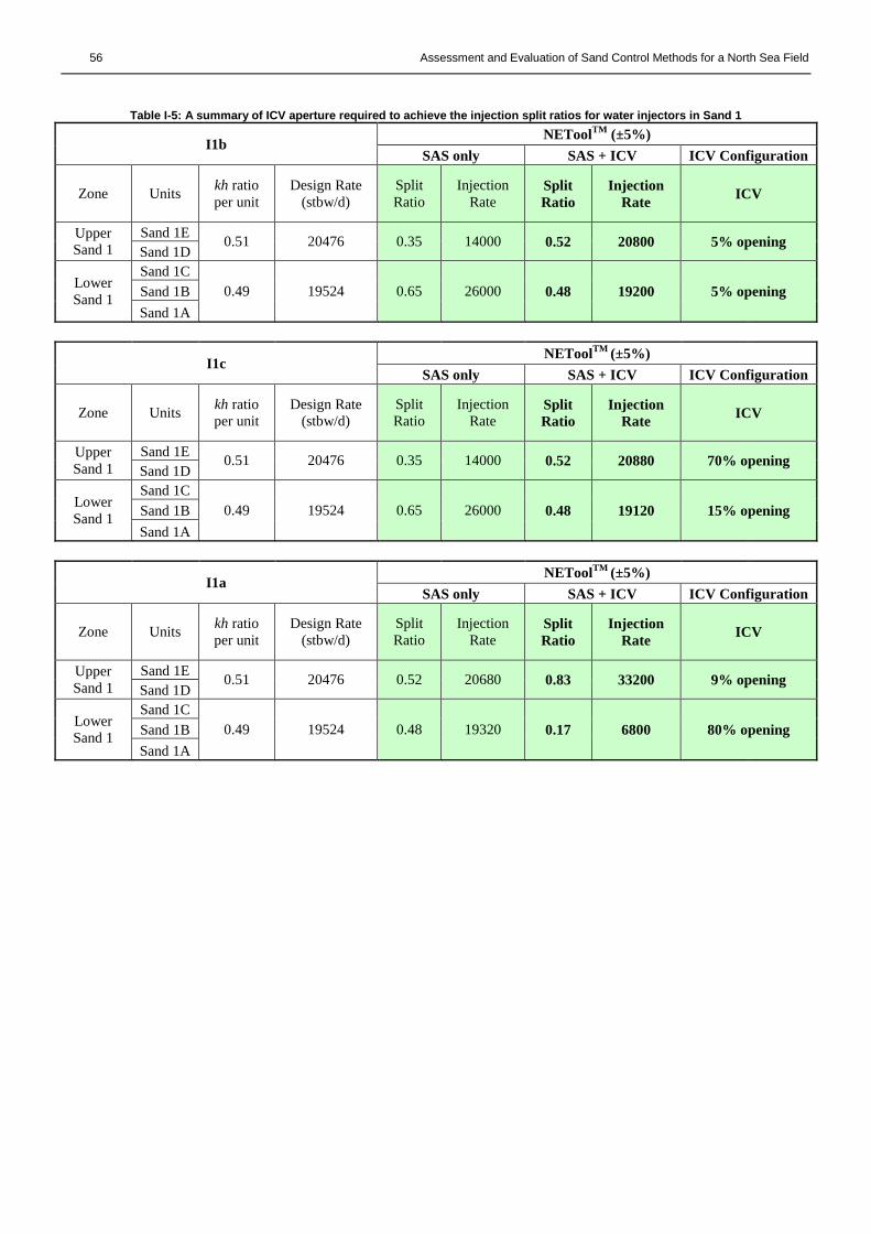
For this case study, I1 and I2 represent the water injectors in Sand 1 and Sand 2 respectively. I1b is used as an example for

this case study and illustrated in Figure 15. Design capacity for this well is 40, 000 stbw/d; which is in the fracture injection

regime. I1b has reservoir drainage of 220 ft. Its kh split ratio is 52% (Upper Sand 1) and 48% (Lower Sand 1). This means the

design injection rates are 20, 700 stbw/d and 19, 500 stbw/d for Upper Sand 1 and Lower Sand 1 respectively. Simulation was

initially conducted with SAS-only completion. The injection profile in SAS-only completion shows 77% of water will be

injected into Upper Sand 1. This creates an uneven distribution of water; meaning ICV will be required to balance the injection

profile. Optimisation of SAS completed with various ICV apertures is sensitised. The outcome of the sensitivity analysis is an

optimised ICV configuration that matches the injection allocations. The results show that both ICVs in I1b with a 5% opening

will give injection rates of 20, 800 stbw/d and 19, 200 stbw/d into Upper Sand 1 and Lower Sand 1, respectively. This shows

injection into Upper Sand 1 can be reduced to 52% of the total injection rate compared to 77% for an SAS-only completion.

This means less water injection into Upper Sand 1 and more water injection into Lower Sand 1. Figure 16 shows the water flux

profile for SAS-only and SAS-ICV completions. The plot shows an improved fluid flow across Sand 1 when ICVs are used.

Barefoot SAS only


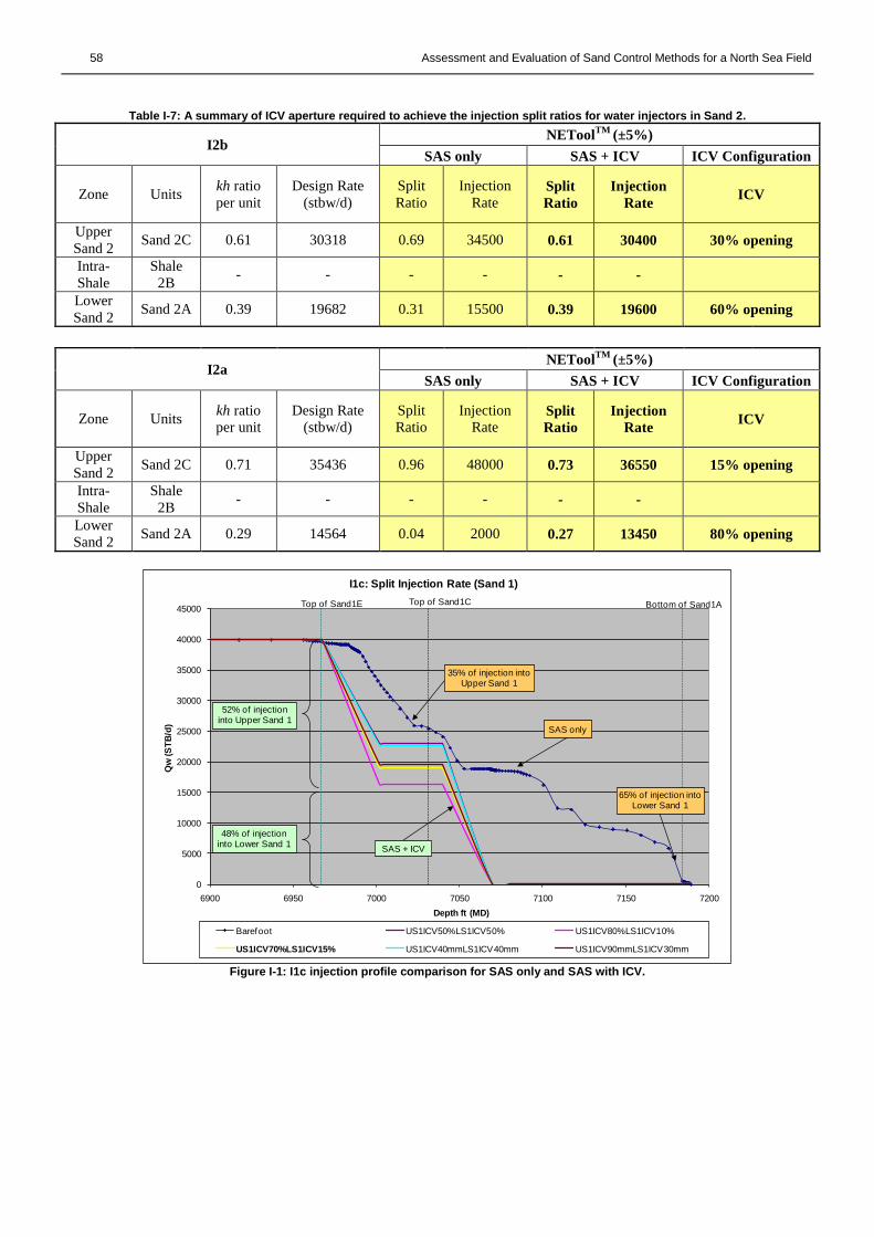
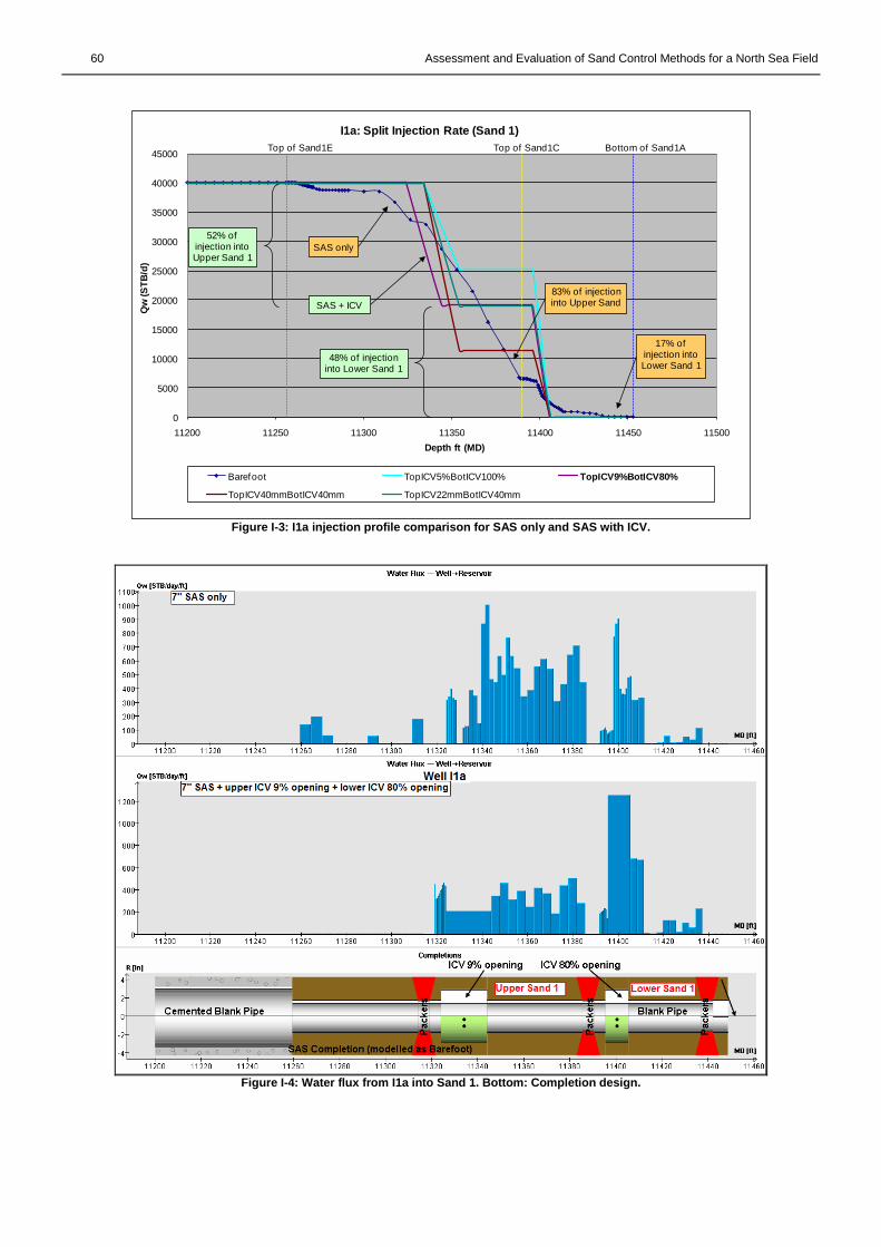
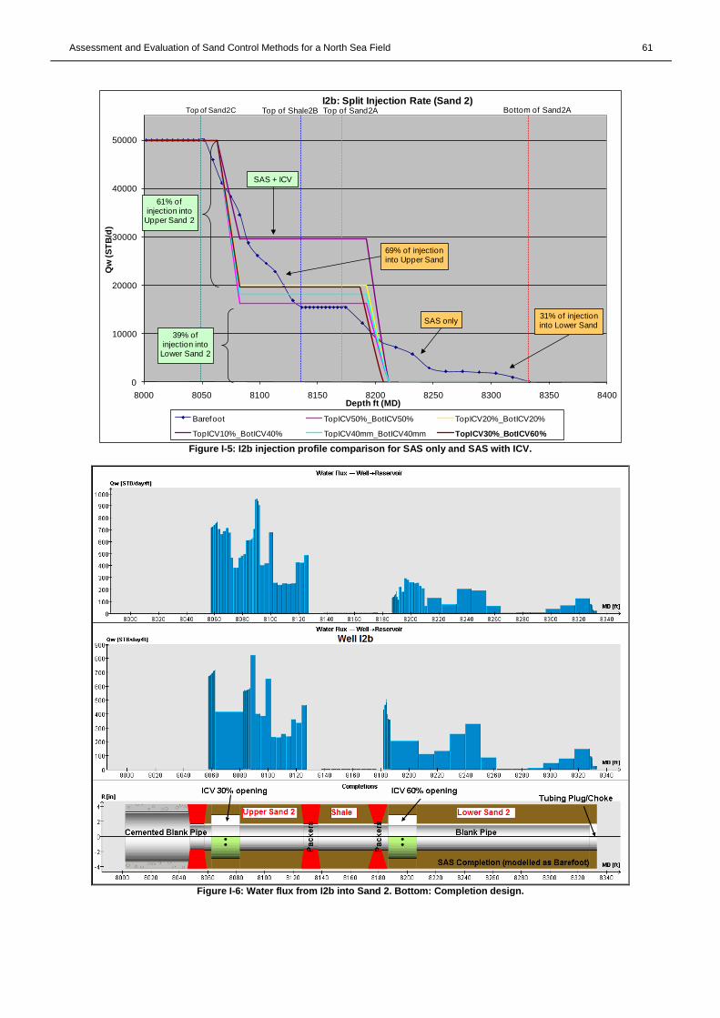
The injection rates based on the optimised ICV for all water injectors are highlighted from Table I-5 to I-7 and the ICV settings

are summarised in Table I-8. Plots to compare injection allocations, water flux profiles and completions for the other five

injectors are in Figure I-1 to I-10.

Top of Sand1E Top of Sand1C Bottom of Sand1A

0

5000

10000

15000

20000

25000

30000

35000

40000

45000

10100 10150 10200 10250 10300 10350 10400

Qw

(S

TB

/d)

Depth ft (MD)

I1b: Split Injection Rate (Sand 1)

Barefoot BothICV100% BothICV20%

BothICV40mmNozzle BothICV20mmNozzle BothICV5%opening

SAS + ICV

52% of WI to Upper Sand

SAS only

48% of WI to Lower Sand

77% of WI to Upper Sand 1

23% of WI to Lower Sand

Figure 15: Split design injection rate into the Upper & Lower Sand 1 for I1b.

In SAS-ICV injectors (Figure 17), water will flow out of the well (blue arrow) and into the annulus (red arrow). Most of the

water will flow into the reservoir whilst the remaining water will flow in the annulus. Sensitivity analysis with water injection

rates at every ten thousand barrels from 10, 000 to 50, 000 stbw/d shows there is some fluid velocity in the space between the

SAS annulus and openhole wellbore.

The annular velocity profile of I1b injector in Figure 18 shows the topmost screen joint (i.e. the heel) is potentially the

weakest point in the completion and the screen is expected to fail first as a result of hot spotting. This effect causes screen

plugging and erosion if the annular fluid velocity exceeds the erosion (threshold) velocity (Ve). The Ve varies among operators

and is controlled by solids content of the injected fluid, fluid particles size and SAS selection (Cameron et al. 2007). Several

references suggested the safe limits of annular flow velocity for WWS and Premium screens are 1 ft/s and 2 ft/s respectively

(Wong et al. 2003).

The maximum annular flow velocity in Figure 18 at the topmost screen joint is 2 ft/s, if the water is injected at 50, 000

stbw/d. At lower injection rates, the effect of annular velocity reduces. Reservoir strategy for this well shows the maximum

injection rate is 24, 000 stbw/d and averages at 12, 000 stbw/d. In this case, the risk of screen erosion caused by hot spots is

minimal. If reservoir management calls for water injection up to 50, 000 stbw/d from I1b, risk of screen erosion is moderate

and still within acceptable limits. The study also shows compartmentalisation using packers have minimal effect on reducing

the annular velocity. This is demonstrated in Figure I-13, where up to four packers were used to isolate and did not reduce the

annular velocity. Sensitivity analyses on the annular velocity of the other water injectors are illustrated from Figure I-11 to

Figure I-13. In summary, Sand 1 has low risk of screen erosion between 10, 000 – 30, 000 stbwd, moderate risk at 40, 000

stbw/d and high risk at 50, 000 stbw/d. Sand 2 has low annular velocity risk for all water injection rates except for the

commingling water injector. The results of the sensitivity analyses are highlighted in Table I-9.


Figure 16: Water flux from well into Sand 1 (Top/Middle: SAS only vs. SAS+ICV). Bottom: Completion design.

Figure 17: Schematic of a typical SAS-ICV completion for this case study

Figure 18: Annular velocity (v) with zonal isolation in the integrated SAS+ICV completion. The circled (red) shows the top most screen

joint is the weakest point of the completion.


Conclusions

A new methodology, this paper recommends sand control selection in a concise and easy to understand manner for six water

injectors in a North Sea field. The methodology is presented as a combination of flowcharts and a sand control selection table

matrix, enabling the engineer to assess the risk of the recommended equipment.

The water injectors are vertical or deviated at less than 30o into the reservoir sections and independent of σH azimuth

orientation. Sand control for all six water injectors in Sands 1 and 2 has been evaluated in accordance to this new methodology

as per below:

Openhole SAS is the preferred technique.

- Premium-type SAS is recommended, because most of the sand has D10 greater than 175 µm, moderately

uniform, and have fines of less than 5%. This option is suitable to accommodate an injection capacity of up

to 50, 000 stbw/d and remain stable under a high rugosity wellbore.

- WWS is not recommended. Prone to fines migration, WWS is susceptible to screen erosion and plugging.

Both reservoirs have fines greater than 2%, exceeding the methodology boundaries that enable them to use

WWS.

OHGP such as LAWP, HAWP and Slurry Pack are not recommended because gravel packs are likely to displace

when injecting at fracture regimes. OHGP also has higher operational risks, and is a more expensive option.

Cased Hole Gravel Pack (CHGP) and High Rate Water Pack (HRWP) are also not recommended as both may suffer

from limited outflow, perforation plugging and high completion skin values. In fact, wellbore stability for this case

study shows that casing is not necessary.

Premium-type SAS utilising blank pipes and packers will be integrated to isolate shale sections. ICV will be included to

even out the non-uniform distribution of water injection, caused by the effects of permeability variation. In addition, NEToolTM

modelling simulates different optimised ICV apertures to match the injection allocations for all water injectors; calculated from

permeability-thickness. Sensitivity analyses at various injection rates shows flow velocity in the screen annulus is below the

critical erosional velocity for Premium-type SAS.

In summary, the methodology is validated and supplemented by risks and concerns. The risks are large permeability

variation and presence of shale in the oil bearing zones. As long as ICV, blank pipes and packers are included to manage the

risks, the use of Premium-type SAS as a sand control equipment for this case study is justified.

Suggestions for Further Work

Expand the methodology further for cased hole sand control

To include sand retention study and design of screen slot sizing in the methodology

Simulate and compare injection flow profiles in the field’s production life.

The evaluation of installing back-flow check valve to reduce the water ‘hammer’ effect when wells are shut-in.

Comparison of injection performance (nodal analysis) for various sand control options using Skin, Injectivity Index

(II) and Completion Efficiency (CE) as the sensitivity parameters.

Nomenclature ∆P Pressure Drop [psi]


bbl/d Barrels per day


CHGP Cased Hole Gravel Pack

D Darcy

D10 Particle Size (10th percentile)




DIF Drill-In Fluids



FMI Formation Image Log

GP Gravel Pack

HRWP High Rate Water Pack

I1 Sand 1 Water Injector

I2 Sand 2 Water Injector

ICD Inflow Control Device

ICV Inflow Control Valves

ID Internal Diameter

kH Horizontal Permeability [mD]

kh Permeability Thickness [md.ft]

k-ø Permeability-Porosity Relationship

kv Vertical Permeability [mD]

kv/kH Vertical-Horizontal Permeability Ratio

LPSA Laser Particle Sieve Analysis

MD Measured Depth

NAF Non Aqueous Fluid

NTG Net to Gross [%]

OBM Oil Based Mud

OD Outer Diameter

OHGP Open Hole Gravel Pack

OM Optical Microscopy

Pfrac Fracture Opening Pressure [psia]

PLT Production Logging Tool


PPS Pre-packed Screen

PSD Particle Size Distribution

R2 Linear Regression

RQI Rock Quality Index


Sc Sorting Coefficient (D10/D95)

SCS Sand Control Selection

SEM Scanning Electron Microscopy

SOBM Synthetic Oil Based Mud


st sidetrack

stbw/d Stock Tank Barrels of Water per Day

TVDSS Total Vertical Depth Subsea

Uc Uniformity Coefficient (D40/D90)

v Annular Fluid Velocity [ft/s]

Ve Critical Erosional Velocity [ft/s]

WBM Water Based Mud

WC Wellbore Condition

WI Water Injector

WWS Wire Wrapped Screen

XRD X-Ray Diffraction

μm Micron

σH Maximum Horizontal Stress Gradient [psi/ft]

σh Minimum Horizontal Stress Gradient [psi/ft]

σv Vertical (Overburden) Stress Gradient [psi/ft]

References Beesley, M. Martin_Beesle[email protected]. Core Grain Size Data and Analysis. 20 June 2011.

Birchenko, V.M., Al-Khelaiwi, F.T., Konopczynski, M.R., Davies, D.R.: "Advanced Wells: How to Make a Choice between Passive and

Active Inflow-Control Completions," paper SPE115742 presented at the 2008 SPE Annual Technical Conference and Exhibition,

Denver, Colorado, USA, Sept. 21-24.

Byrne, M., Slayter, A., McCurdy, P.: "Improved Selection Criteria for Sand Control - When Are "Fines" Fines?," paper SPE128038

presented at the 2010 SPE International Symposium and Exhibition on Formation Damage Control, Louisiana, USA, Feb. 10-12.

Cameron, J., Jones, C.: "Development, Verification and Application of a Screen Erosion Model," paper SPE107437 presented at the 2007

Scheveningen, The Netherlands, May 30-June 1.

Coberly, C.J.: "Selection of Screen Openings for Unconsolidated Sands," API. Drilling and Production Practice (1937).

Farrow, C., Munro, D., McCarthy, T.: "Screening Methodology for Downhole Sand Control Selection," paper SPE88493 presented at the

2004 SPE Asia Pacific Oil and Gas Conference and Exhibition, Oct. 18-20.

Franklin, A.J. Andrew.[email protected]. Sand screen opening. 8 August 2011.

Gorden, W.C. will[email protected]. Fracture orientation. 20 June 2011.

Khalil, A., Elasmar, M., Shafie, S.: "Optimizing Injection Wels through Innovative Completion," paper SPE137057 presented at the 2010

Abu Dhabi International Petroleum Exhibition & Conference, Abu Dhabi, UAE, Nov. 1-4.

Price-Smith, C., Parlar, M., Bennett, C., Gilchrist, J.M., Pitoni, E., Burton, R.C., Hodge, R.M., Troncoso, J., Ali, S.A., Dickerson, R.:

"Design Methodology for Selection of Horizontal Openhole Sand-Control Completions Supported by Field Case Histories," paper

SPE85504 presented at the 2000 SPE European Petroleum Conference, Paris, Oct. 24-25.

Prior, N., Coates, I., Beesley, M.: "Case Study Area Development: Geomechanical Model Update and Sanding Prediction Study", CC328-

11/R1/730, Issue 2, September 2010.

Saucier, R.J.: "Considerations in Gravel Pack Design," JPT (Feb. 1974) 205-212.

Slayter, A.G., Byrne, M., McPhee, C.A., McCurdy, P.: "Sand Management: What Are We Sure Of?" paper SPE114781 presented at the

2008 SPE Asia Pacific Oil & Gas Conference and Exhibition, Perth, Australia, Oct. 20-22.

Svendson, A.P., Wright, M.S., Clifford, P.J., Berry, P.J.: "Thermally Induced Fracturing of Ula Water Injectors," SPE Production

Engineering (Nov. 1991) 6.

Tiffin, D.L., King, G.E., Larese, R.E., Brit, L.K.: "New Criteria for Gravel and Screen Selection for Sand Control," paper SPE39437

presented at the 1998 SPE Formation Damage Control Conference, Lafayette, LA, Feb. 18-19.

Tolan, M., Tibbles, R.J., Alexander, J., Wassouf, P., Schafer, L., Parlar, M.: "Gravel Packing Long Openhole Intervals with Viscous Fluids

Utilizing High Gravel Concentrations: Toe-to-Heel Packing Without the Need for Alternate Flow Paths," paper SPE121912 presented

at the 2009 Asia Pacific Oil and Gas Conference & Exhibition, Indonesia, August 4-6.

White, M.J. Martin_Whit[email protected]. Nearby Asset Sand Evaluation Study. 20 June 2011

Wong, G. K., Fair, P.S., Bland, K.F., Sherwood, R.S.: "Balancing Act: Gulf of Mexico Sand Control Completions, Peak Rate Versus Risk of

Sand Control Failure," paper SPE84497 presented at the 2003 SPE Annual Technical Conference and Exhibition, Denver, Colorado,

Oct. 5-8.

Xiang, W., Wang, P.: "Application of Bridging Theory on Saucier Gravel to Examine the Sand Control Effect," SPE80450 presented at the

2003 SPE Asia Pacific Oil and Gas Conference Exhibition, Jakarta, Indonesia, Sept. 9-11.

Yale, D.P., Rodriguez, J.M., Mercer, T.B., Blaisdell, D.W.: "In-Situ Stress Orientation and the Effects of Local Structure-Scott Field, North

Sea," paper SPE28146 presented at the 1994 Eurock SPE/ISRM Rock Mechanics in Petroleum Engineering Conference, Delft, The

Netherlands, Aug. 29-31.

APPENDICES


APPENDIX A: CRITICAL LITERATURE MILESTONES TABLE

Paper Year Title Authors Contribution 58-066

(API)

1958 “Sand Exclusion in Oil and

Gas Wells”

G.H.Tausch, C.B.Corley First to discuss the theory and methods of sand

exclusion i.e. bridging and consolidation of sand

grains.

2330

1968

“Successful Sand Control

Design for High Rate Oil and

Water Wells”

D.H.Schwartz

1. First to describe sand control design procedure

for oil producer and water injector wells.

2. First to present methods for designing gravel

packed completion.

39437

1998

“New Criteria for Gravel and

Screen Selection for Sand

Control”

D.L.Tiffin, G.E.King,

R.E. Larese, L.K.Amoco

1. First to present guidelines for sand control

completion technique and gravel size selection

based on reservoir sand size distribution.

2. Consolidated proposed design criteria based on

field experience and experiments on cores from

various formations.

85540

2003

“ Design Methodology for

Selection of Horizontal

Openhole Sand-Control

Completions Supported by

Field Case Histories”

C.Price-Smith, C.Bennett,

J.M.Gilchrist, E.Pitoni,

R.C.Burton, R.M.Hodge,

J.Troncoso, S.A.Ali,

R.Dickerson

1. First to propose a generalized and unified

methodology for determining when, what and how

to install horizontal openhole completions.

2. Presented a risk analysis by integrating all

relevant factors.

88493 2004 “Screening Methodology for

Downhole Sand Control

Selection”

C.Farrow, D.Munro,

T.McCarthy

First to propose a methodology incorporating a

combination of flowchart and sand control selection

matrix.

93564 2005 “Designing Effective Sand

Control Systems to Overcome

Problems in Water Injection

Wells”

H. Sadrpanah, R. Allam,

A.Acock, M.Norris,

T.O’Rouke

1. First to provide guideline in selecting and

designing sand control systems for water injector

wells.

2. Summaries causes of sand control failures based

on detailed case studies.

106018 2007 “ICD Screen Technology

Used To Optimize

Waterflooding in Injector

Well”

A.G. Raffn, S. Hundsnes,

S. Kvernstuen, T. Moen

Propose an innovative completion of inflow control

technology with sand control screens for injection

wells

107539 2007 “Successful Installation of

Stand Alone Sand Screen in

More Than 200 Wells – The

Importance of Screen

Selection Process and Fluid

Qualification”

A.M.Mathisen, G.L.

Aastveit, E. Alteras

1. First to recommend a sand control selection

practice based on comprehensive screen selection

and fluid qualification process.

2. First to publish testing and ranking of different

screen designs based on sand retention and

plugging properties.

112283 2008 “Equalization of the Water

Injection Profile of a Subsea

Horizontal Well: A Case

History”

A.S. Amaral, J.

Augustine, K. Henriksen,

V.F.,Rodrigues,

D.E. Steagal,

L.C.A.Paixao

First global installation of a water injector well with

a lower completion system that include both

premium sand control screens and inflow control

technology to equalize injection profile.

114781

2008

“Sand Management: What

Are We Sure Of?”

A.G. Slayter, M.Byrne,

C.A. McPhee, P.McCurdy

First to propose a methodical framework with

defined objectives, tasks and activities for the

execution and qualification of sand control design

128038

2010

“Improved Selection Criteria

for Sand Control – When Are

“Fines” Fines?”

M.Byrne, A.G. Slayter,

P.McCurdy

First to redefine classification of “fines” by

considering the impact it has on the formation and

its ability to move through the pores of unperturbed

rock

137057 2010 “Optimizing Injection Wells

through Innovative

Completion

A. Khalil, M. Elasmar, S.

Shafie

First to apply influx control device (ICD) in an

injector well for carbonate formation.


APPENDIX B: CRITICAL LITERATURE REVIEWS

API 58-066, 1958

First presented during a meeting at the Southern District, Division of Production, Houston, Texas, February 1958.

Title: Sand Exclusion in Oil and Gas Wells

Authors: Tausch, G. H., Corley C. B. Jr.

Contribution to the understanding of sand control concept selection: This paper describes the two general methods of sand

control. The methods are 1) bridging of sand grains and 2) consolidation of sand in place. Each method also describes the

design criteria required when selecting a sand exclusion technique.

Objective of the paper: A detailed examination of sand exclusion techniques. The techniques studies are slotted/wire-

wrapped screen, gravel packing, plastic coated walnut shells and plastic consolidation.

Methodology used: The bridging of sand grains is controlled by the size of the openings in the standalone screen and gravel

pack. The size of the openings is determined by analysing the D10 sieved from dry analysis. The D10 i.e. the formation sand

sizing grain diameter is an important criterion for the design of the bridging method. Consolidation of grains uses plastic

material and the critical design criteria are formation permeability and temperature instead.

Conclusion reached: Bridging techniques can be applied on initial completion and consolidation techniques after completion

(i.e. when there is an indication of formation sand produced). Both techniques have different design criterion.

Comments: This paper unifies sand control techniques into two techniques for both oil and water-producing wells. For the

bridging method, the paper describe slotted line, wire wrapped screens and gravel pack as the solution. Detailed design and

effectiveness of the sand control equipment was only briefly discussed. The grain size analysis focussed only on the minimum

formation size (D10) for the screen slot design.


Journal of Petroleum Technology, September 1969

Presented at the SPE 39th

Annual California Regional Fall Meeting held in Bakersfield, USA 7-8 November, 1968

Title: Successful Sand Control Design for High Rate Oil and Water Wells

Authors: Schwartz, D. H.

Contribution to the understanding of sand control concept selection:

Objective of the paper: To present a technique for designing gravel flow packed liner completion. Design criteria are

formation analysis, gravel-to-sand ratio and velocity through slots. The objective is to design a sand control for high rate oil

producer and water injections wells. Subsequently, a sand control design is recommended that is sufficient to last through

secondary recovery projects (~ 10 years).

Methodology used: Describes the Tyler Standard Screen Scale (sieve analysis) to measure the grain diameter (Dx) and

uniformity coefficient (C). Dx refers to the sieve size distribution (cumulative, %). C is determined from the slope of the sieve

analysis:

C = D40/D90

The equation above shows a sieve opening at which 40% of the sand is being retained divided by another sieve opening at

which 90% of the sand is being retained. Below is the description of the C value:

C < 3: Uniform Sand

C > 5: Non-uniform sand

Describes the parameter of the Gravel-to-Sand Ratio (G-S) i.e. the gravel grain size to the formation sand grain size:

- G-S ≤4 will give a stable pack

- G-S between 10 and 13 will give an unstable pack due to the invasion of formation into the pack

- G-S between 6 and 8 will give the most optimum design

The final methodology describes the effects of velocity towards the gravel flow pack. Increasing velocity will tend to destroy

the pack stability. A design curve was plotted in determining the gravel and formation critical grain size for the design of the

gravel and screen opening respectively.

Conclusion reached: Successful and control design can be achieved by defining the sand, gravel design and quality of control

of gravel once it is in place.

Comments: The paper provided some understanding of how to measure the sand grains from sieve analysis. The methodology

focuses solely on gravel pack techniques.


SPE 39437, 1998

This paper was presented at the 1998 SPE Formation Damage Control Conference held in Lafayette, LA, 18-19 February

Title: New Criteria for Gravel and Screen Selection for Sand Control

Authors: Tiffin, D.L., King, G. E., Larese, R. E., Britt L. K.

Contribution to the understanding of sand control concept selection: A proposed criterion has been published focussing

primarily on reservoir sand size distribution. The criterion methodology focuses on the distribution of the grain sizes in terms

of sorting. The study also evaluates the concerns of formation with very high fines content. Methodology uses field experience

and experiments on reservoir cores worldwide as part of the study.

Objective of the paper: To propose a new sorting criteria and completion techniques relating to the selection of gravel and

screen size. The proposed criterion focuses on sorting techniques and mobility of fines.

Methodology used: Added a new piece of design information to the commonly used Saucier’s criteria for screen and gravel

size selection. Design methodology uses D50, D40/D90, D10/D95 and mobility of fines particles for sand control selection. If

D50 < 75μm, gravel pack is preferred as fines constitutes a large portion of the sand distribution making screens impractical .

The D10/D95 is a new criterion and used to distinct variation between the size and sorting ranges of formation sand.

Conclusion reached: The proposed criteria for evaluating formation sand sorting values are presented below:

Table B-1: Formation Sand Sorting Values

Sorting Proposed Purpose

D50 Standard Saucier Criteria

D40/D90 Screen Damage Ratio from Pall

D10/D95

Size range between common

minimum and maximum particle

sizes

Sub 325 mesh Quantity of sub 44micron

particles (fines)

Several case studies were conducted using the methodology and summarised below:

Table B-2: Proposed Sorting Criteria

Completion Techniques D40/D90 D10/D95 Sub 325

mesh (fines)

Bare screen <3 <10 <2%

Bare screen with woven

mesh screens <5 <10 <5%

Gravel placed in high rate

water pack <5 <20 <5%

Gravel and Fines-passing

screen <5 <20 >10%

Enlarge the wellbore through

fracturing or horizontal/

multilateral well

>5 >20 >10%

Comments: This paper presents a solid method in determining the screen and gravel size selection. It highlights the various

sorting methods and most importantly the concern of fines mobility. The summary of case studies tabulated above provides a

much better understanding of what type of sand control is needed based on the formation sand size distribution. This study also

highlights the need to enlarge the wellbore if large quantity of fines is present.


SPE 85504, June 2003

This paper was first presented at the 2000 SPE European Petroleum Conference held in Paris, France, 24-25 February. The

paper was revised for publication from paper SPE 65140.

Title: Design Methodology for Selection of Horizontal Openhole Sand-Control Completions Supported by Field Case

Histories

Authors: Price-Smith, C., Parlar, M., Bennet, C., Gilchrist, J. M., Pitoni, E., Burton, R. C., Hodge, R. M., Troncoso, J., Ali, S.

A., Dickerson, R.

Contribution to the understanding of sand control concept selection: This paper discusses a unified methodology for

determining the type of sand control needed for openhole horizontal completions. It highlights a step-by-step guide from

predicting sand to establishing the type of sand control needed. The criteria in determining the type of sand control is based on

field experience, knowledge and experimental data. This paper also provided a range of critical design criterion when selecting

a sand control technique from a range screens and gravel packs available to date. The criterion includes deepwater and non-

deep water environments. Several case histories were applied to support the methodology proposed.

Objective of the paper: To propose a unified and well-defined set of guidelines for selecting a sand control technique. The

paper provides specific factors that links ‘when’, ‘what’ and ‘how’ to install sand control in openhole horizontal completions.

Methodology used: In deepwater environments (>1500ft), the cost of intervention outweighs the sensitivity cost of screen

selection and gravel pack (GP). For non-deep water environments (<1500ft), initial screening uses formation sand size

distribution as per Tiffin criteria. The methodology describes the presence of shale in productive sand requires isolation

through the use of blank pipes or mechanical inflatable packers.

The methodology highlights in detail the design criterion that affects the type of gravel pack. Two types of GP are commonly

used: GP-Water Pack and GP-Shunt Pack. The use of GP-Water Pack depends primarily on the pay length, shale content/

reactivity and drilling fluid compatibility. GP-Water Pack is preferred over GP-Shunt pack when the formation sand is uniform

and NTG is high i.e. > 60-80%. Depending on the scenario, GP-Shunt Pack is preferred in high-risk environments because the

success ratio for this method is 100%.

The methodology also highlights several critical concerns before and after installing a sand control technique. Details of the

methodology are presented in table formats. The proposed methodology was checked and compared against 10 case studies.

Conclusion reached: The methodology (unified set of guidelines) should be use cautiously and requires further validation and

refining when selecting the most appropriate sand control. Based on the validating methodology with the case studies, the

results is summarised below: Table B-3: Sand Control recommended using Price-Smith et al. methodology

Median Grain Size

(D50)

Uniformity

(D40/D90)

Fines

content

Production

Rate Sand Control Recommended

> 75μm High Low Low Wire Wrapped Screen

> 75μm Moderate Moderate Low Prepacked Screen or Premium Screen

> 75μm High Low High

Prepacked Screen or Premium Screen

(Large screen OD required to minimize

annular flow)

- Use gravel pack when D50< 75μm. GP-Shunt Pack is recommended for low NTG, reactive shale, OBM and low

fracture gradient. GP-Water Pack is for high NTG, absence of reactive shale, WBM and high fracture gradient

environments.

- For deepwater environment (i.e. intervention cost outweighs sand control cost), the most reliable sand control

technique must be used.

Comments: This paper gives a detailed overview over a range of design criteria that needs to be conducted prior to choosing

the suitable sand control. Further design criterion is added in this paper such as the presence and reactivity of shale, NTG and

depth of water. The paper has unified a unique methodology when selecting a sand control technique compared to other

published papers. The ten case studies focused on horizontal openhole completions but did not use well length as a design

criterion.


SPE 88493, October 2004

This paper was presented at the 2004 SPE Asia Pacific Oil and Gas Conference and Exhibition held in Perth, 18-20 October

Title: Screening Methodology for Downhole Sand Control Selection

Authors: Farrow, C., Munro, D., McCarthy, T.

Contribution to the understanding of sand control concept selection: This paper introduces a sand control selection matrix

using a traffic light output system. The system ranks available sand control techniques based on likelihood and consequences.

The likelihood factor is based on a range of design criteria and the consequences factor is related to risks.

Objective of the paper: To develop a screening methodology by evaluating and ranking of available sand control techniques.

The methodology incorporates a combination of a flowchart and a sand control selection matrix.

Methodology used: The flowchart is used for initial screening. It addresses which sand control options are suitable. The

flowchart highlights the type, location and deviation of the well under study.

Figure B-1: The proposed initial selection flowchart and sand control ‘traffic light’ selection output.

The above figure on the right indicates sand control techniques vs. design criteria. The matrix uses a colour code output.

Green represent no concerns, yellow = some concern, orange = significant concern and red = ruled out. Any sand control

techniques that receives red are eliminated immediately. Remaining sand control options are then evaluated by comparing the

colour output of other design criteria.

Selection matrix includes additional design criteria in the sand control selection. The criteria are reservoir length, reservoir

fluid characteristics and production performance. Well intervention, cost, reliability and installation are risks criteria that are

also included in the matrix. Methodology has been applied on three case studies. Case study 1 and 2 are cased-hole wells on

existing platforms. Case 3 is an open-hole well for a sub-sea development. Gravel pack and standalone screen are the

recommended sand control option for the former and latter respectively.

Conclusion reached: Screening methodology using the flowchart and the selection matrix enables transparent evaluation and

balanced ranking of sand control options. Additional critical design criteria on top of the common ones are highlighted.

Comments: This paper gives a unique methodology for sand control selection. Output of the methodology can be evaluated

and compared with established sand control techniques for a particular area. It uses a range of design criteria and requires input

from static and dynamic perspective. To date, this is the best methodology to yield the optimum sand control.


SPE 106018, April 2007

This paper was presented at the 2007 SPE Production and Operations Symposium held in Oklahoma City, Oklahoma, USA, 31

March-3 April

Title: ICD Screen Technology Used To Optimize Waterflooding in Injector Well

Authors: Raffn, A.G., Hundsnes, S., Kvernstuen, S., Moen, T.

Contribution to the understanding of sand control concept selection: This paper highlights the use sand controlled screens

with integrated flow control devices for open-hole completed water injectors. It discusses the risk of erosion and plugging on

the screens caused by the irregular flow distribution due to large permeability variation in the formation.

Objective of the paper: To present an innovative completion with sand control and inflow control devices to improve water

injection profiles in various sand formation zones. It is modelled and tuned using reservoir stimulations.

Methodology used: The completion consists of wire-wrapped sand screen with inflow control device. The test was to

understand flow and erosion on injector wells with screens and ICD. Flow is based on Bernoulli equation:

Pressure drop is generated by fluid flow through the nozzles. The relationship above shows ICD is used to restrict and

stimulate flow into high and low permeability zones respectively; providing a much inflow distribution of water into the

permeable zones.

Conclusion reached: Stimulation runs identify the possibility of controlling injection rates into individual zones. This paper

also highlights that ICD injector completion is significantly less influenced by permeability contrasts compared to a standard

screen completion.

Comments: Nothing significant. However, the paper gives a good understanding that injected fluids prefers to flow into high

permeability streaks; leading to early breakthrough and poor recovery that must be prevented


SPE 107539, June 2007

This paper was presented at the 2007 European Formation Damage Conference held in Scheveningen, The Netherlands, 30

May-1 June

Title: Successful Installation of Stand Alone Sand Screen in More Than 200 Wells – The Importance of Screen Selection

Process and Fluid Qualification

Authors: Mathisen, A.M., Aastveit, G. L., Alterås, E.

Contribution to the understanding of sand control concept selection: This paper highlights the failure of active sand

control caused by long shale sections, high content of fine material and incompatibility of completion fluids to the formation.

Objective of the paper: To recommend a practice based on comprehensive screen selection by testing and ranking of

different screen designs. The study includes a fluid qualification process by ensuring the drilling and completion fluid is

compatible during the sand screen installation.

Methodology used:

1) Sand retention and screen plugging testing were used to rank the screen designs as part of the sizing selection. Data for the

tests were collected from the formation’s weakest and poorest uniformity/sorting coefficients. The preparation of the data was

originally from sand failure studies and particle sand distribution (PSD). The PSD analysis was plotted using dry sieve analysis

and quality checked with Laser Particle Size Analysis (LPSA). Wire-Wrapped, Premium and Expandable screens were used

for the tests.

2) Geological evaluation on the reservoir heterogeneity was used to identify shale sections between the core and the planned

well path. The outcome of the evaluation determines the number of blank pipers and/or packers required to isolate unstable

shale sections.

3) Inflow control technology was recommended to minimise annular flow. This phenomena transports particles in the annular

hence increases the risk of screen plugging. The paper highlights the use of inflow control device (ICD) to reduce annular flow

and provide a uniform inflow profile across the horizontal section of a well. Blank pipes and packers are also used to reduce

annular flow.

Conclusion reached: Sand retention and plugging studies shows Premium screens has the lowest pressure drop combined

with high sand retention and permeability. Inflow control technology and isolation devices are recommended for formations

with long shale sections and/or high content of fine material.

Comments: This paper provides a comprehensive ranking on various screen designs using formation sand properties. It

highlights the importance of sand retention and screen plugging even though it is conducted only at laboratory conditions. The

paper also gives a brief justification of using inflow control technology and isolation devices as part of the sand control

selection.


SPE 112283, February 2008

This paper was presented at the 2008 Formation Damage Control held in Lafayette, Louisiana, 13-15 February 2008

Title: Equalization of the Water Injection Profile of a Subsea Horizontal Well: A Case History

Authors: Amaral, A. S., Augustine, J., Henriksen, K., Rodrigues, V.F., Steagal, D.E., Paixão, L.C.A., Barbosa, P.

Contribution to the understanding of sand control concept selection: This paper focuses on the installation of water

injector well with a lower completion system that incorporates both premium sand control screens and profile equalization. A

schematic of the injector completion details was presented.

Objective of the paper: To create a uniform outflow profile in sand controlled completions for subsea horizontal water

injectors.

Methodology used: Sand controlled completions such as standalone screens do not provide equalization of the water injection

profile. An open-hole gravel pack provides some equalization but is affected by cost, risk and complexity.

Water injector well locations were defined and reservoir stimulation with desired injection rates was achieved. The stimulation

shows uniform injection is required along the horizontal section. This is to prevent water-fingering and early breakthrough.

Injection profiles at various injection rates were therefore stimulated. Severe imbalance of water influx into the reservoir was

observed at the heel section of the horizontal water injector when non-equalizing sand controlled completion was used.

Completion with screens and equalization provides a much better distribution of injected water into the horizontal section (i.e.

heel to toe) of the well.

Conclusion reached: The use of equalization, screens and isolation packers enhances and improves water injection profile. It

eliminates the chance of annular flow occurring.

Comments: This paper highlights inflow control devices can be used with sand controlled screens if equalize outflow profile

is required in a water injector well. However, the findings are based only on a subsea horizontal well.


SPE 114781, October 2008

This paper was presented at the 2008 SPE Asia Pacific Oil & Gas Conference and Exhibition held in Perth, Australia, 20-22

October

Title: Sand Management: What Are We Sure Of?

Authors: Slayter, A. G., Byrne, M., McPhee, C. A., McCurdy, P.

Contribution to the understanding of sand control concept selection: This paper highlights best practice on several design

criteria for openhole wells that require sand control. Rock mineralogy, particle size distribution (PSD), screen-to-openhole

annulus, screen failure mechanisms and screen collapse/ buckling are the design criteria discussed.

Objective of the paper: To propose a systematic framework to address critical design criteria in a timely and ordered manner.

Sand control design criteria usually tangled with more than one objective.

Methodology used: 1) Rock mineralogy study: Used X-Ray Diffraction (XRD) to identify the presence and type of clays. Cation Exchange

Capacity (CEC) is used to measure the reactivity of shale (i.e. swelling of clays). Dynamic Flow through Test

(DTTT) is part of the study to assess the clay behaviour when fluids are circulated at high rates through a core

sample. This study is important to determine the compatibility of water-based mud (WBM) for gravel water packs.

Table B-4: Typical CEC values for specific clays

Type & Behaviour of Clay CEC meq/100g)

Swelling Smectites 80-150

Mobile Kaolinites 1-10

2) PSD study: Laser Particle Sieve Analysis must be performed on top of the dry sieve analysis. This is to quality check

the particle size distribution from both techniques. Fines are its ability to move between pores of a rock. Rock grain

sizes smaller than 325mesh (44µm) are categorised as fines. The 44 µm cut-off is based on the finest sand screen

available to date. Fines greater than 10% is a concern for all sand control options. The study recommends wellbore

enlargement and this proposal is consistent with Tiffin’s criteria.

3) Screen-to-Openhole Annulus study shows annular removal is necessary to prevent flow behind the pipe. This will

prevent screen erosion and plugging caused by hot spots and fine particles respectively. Flow in the annular can be

prevented by using inflow control devices (ICD) and expandable annular packers. Significant cost reduction as

opposed to wellbore enlargement. The presence of annular can also be removed by using ESS.

4) Screen failure mechanisms are plugging and erosion. Critical erosion velocities are. Determined. Allowable critical

flow rates for both liquid and gas flow are tabulated below. This is based on consolidation from various operators:

Table B-5: Critical flux rates to avoid erosion for various sand control completions

Sand Control Screen System Critical V for Liquid (ft/s) Critical V for Gas

Flow (ft/s) Company

Expandable Sand Screen (ESS) 1 1 Weatherford

Wire Wrapped Screen (WWS) 1 6 US Filter, Johnson Screen

Woven and Wire Wrapped Screen 1 Not available Shell

Cased Hole Gravel Pack (CHGP) 10 20 BP

5) Screen collapse/ buckling can occur when screen is plugged. This can be mitigated if the well is bean up slowly after

being idle for unknown period of time. The presence of shale is the likely cause of screen plugging because shale is

unstable and brittle. It will weaken and collapse onto sand screen. This increases the likelihood of screen failure.

Conclusion reached: Successful sand management requires an organised approach when executing all design selection

criteria. The use of ICDs and packers must be evaluated as part of a continuous approach in developing optimum sand control

system.

Comments: The paper highlights additional information that is very useful in defining the selection criteria. More focus the

critical design and limitation of sand control screens. Expandable sand screen (ESS) was introduced to remove annular space

in the wellbore. Critical flow rates are useful to minimise screen erosion. Flow rates in the annulus can be lowered by

installing flow control devices and isolation packers as part of the sand control completion.


SPE 128038, February 2010

This paper was presented at the 2010 SPE International Symposium and Exhibition on Formation Damaged held in Perth,

Australia, 20-22 February.

Title: Improved Selection Criteria for Sand Control – When Are “Fines” Fines?

Authors: Byrne, M., Slayter, A. G., McCurdy, P.

Contribution to the understanding of sand control concept selection: This paper highlights new definition of fines. This is

to ensure an optimum and tailored sand control is selected. A modified sand control selection process to account the new

definitions is proposed in this paper.

Objective of the paper: To provide a discussion on fines. It explains how fines should be measured, classified and

interpreted. The paper also reviews previous published literature on fines and existing sand control selection guidelines.

Methodology used: Initial review shows conventional guidelines used in determining sand control systems were Schwartz

(1969) and then Tiffin et al. (1998). Both of the methodology with some additional guidelines were consolidated and

integrated into a flowchart. The definition of fines as “less than 44 µm” is inappropriate for sand control selection in very fine

grained rocks because it may have a high percentage of “less than 44 µm fraction”. The new definition of fines is presented in

the left flowchart below. With the modified definition of fines, the right flowchart presents an enhanced sand control selection

process:

Figure B-2: Definition of fines

Conclusion reached: The paper highlights the meaning of “fines” from an engineering perspective. It redefines fine from

being “less than 44µm” to “to be considered as part of the rock that can move through the pores of intact rock”. A clear

distinction is made between fines moving in intact rock and fines present in the rock that collapsed between the formation face

and the sand control completion.

Comments: This paper provides an engineering view of defining fines for sand control. The flowcharts are useful to find the

true meaning of fines during the sand control selection. It is useful because if the formation fails and deposit into the annulus,

the sizing of fines will be different and further study will be required.


SPE 137057, November 2010

This paper was presented at the 2010 Abu Dhabi International Petroleum Exhibition & Conference held in Abu Dhabi, UAE,

1-4 November.

Title: Optimizing Injection Wells through Innovative Completion

Authors: Khalil, A., Elasmar, M., Shafie, S.

Contribution to the understanding of sand control concept selection: None. However, the inclusion of inflow control to

achieve uniform injection profile in water injectors is required.

Objective of the paper: To share its application of influx control device (ICD) for an injector well for in a carbonate

formation. The completion shows an intelligent wellbore completion that gives an even distribution of injected water along the

wellbore (heel to toe).

Methodology used: Initial review shows heel-to-toe effects, permeability contrasts and existence of fracture thieves are causes

of imbalance water injection profile into the reservoir. Stimulation was modelled to estimate the water injection distribution.

Case A and Case B were run. Case A is a barefoot (no inflow control) completion. Case B is a completion completed with

inflow control. Study was conducted on both cases using a wellbore hydraulics stimulator.

The requirement injection split ratio into the reservoir is 40% (heel):60% (toe). The barefoot completion (Case A) failed to

honour the requirement split ratio. Most of the water injected took the path of least resistance and flowed into the high

permeability zones, located near the heel section of the well. Sensitivity runs was conducted for Case B to achieve the

optimized completion. The optimized completion indeed honoured the design injection split ratio. It provided a much better

distribution of injected water from the heel to the toe section of the well.

Injection log was then conducted and the injected split ratio with the optimized completion was 44% (heel):56% (toe); closed

to the design requirement modelled in the wellbore hydraulic stimulator

Conclusion reached: Most of the injected water will take the path of least resistance and flow into a higher permeable zone;

causing early water breakthrough and poor reservoir sweep of the oil.

Comments: This paper provides a good background on how to model and optimize inflow control devices with sand

controlled completion in a wellbore hydraulic stimulator.


APPENDIX C: NOMENCLATURE

∆P Pressure Drop [psi]


BHT Bottom Hole Temperature


DIF Drill-In Fluids


ECD Equivalent Circular Density


FG Fracture Gradient

FMI Formation Image Logs

GP Gravel Pack

HRWP High Rate Water Pack

ICD Inflow Control Device

ICV Inflow Control Valves

ID Internal Diameter

LPSA Laser Particle Sieve Analysis

NAF Non Aqueous Fluid

NNW North-North West Direction

NTG Net to Gross [%]

OBM Oil Based Mud

OD Outer Diameter

Pfrac Fracture Opening Pressure [psia]

PLT Production Logging Tool

PP Pore Pressure

PSD Particle Size Distribution

PPS Pre Packed Screen

RQI Rock Quality Index


SCS Sand Control Selection

SOBM Synthetic Oil Based Mud


SSE South-South East Direction

WBM Water Based Mud

WC Wellbore Condition

WI Water Injector

WWS Wire Wrapped Screen


APPENDIX D: METHODOLOGY

0

10

20

30

40

50

60

70

80

90

100

1.0010.00100.001000.0010000.00

Cu

mu

lati

ve w

t%


Sand 2C in Well Dst1 @ 7397ft MD: Dry Sieve Analysis PSD

D90=94μm

D40=247μm

D50=214μm

LPSA - Finer end of the PSD (<44μm)

Figure D-1: PSD for Sand 2C in Well Dst1

Table D-1: Sand Control Selection Table for various types of Standalone Screens (SAS)

SAS Preferred Acceptable Use With Caution Not Recommended

Low Fracture Gradient High Rugosity/Severe Washout Deviation 0-55o

Prone to fines migration

High Leakoff Concerns Deviation 55o-75

oNTG < 60-80% Use of breakers

Small Bore Hole ID < 6" High production rate Multiple oil bearing zones

isolated by non-productive

barriersDrill with OBM High frequency of well intervention High Variable Permeability/

Lamination

Drill with WBM/ SOBM Risk of installing equipment

Unstable/ Reactive shale Equipment lifespan/ reliability

High static BHT

Horizontal length 0 - 4000ft, >4000ft

High depleted reservoir

Cost effectiveness

Low Fracture Gradient High Rugosity/Severe Washout Deviation 0-55o


High Leakoff Concerns Deviation 55o-75

oNTG < 60-80% Use of breakers

Small Bore Hole ID < 6"

High production rate

Multiple oil bearing zones


barriers

Drill with OBMHigh frequency of well intervention

High Variable Permeability/

Lamination

Drill with WBM/ SOBM Risk of installing equipment Equipment lifespan/ reliability

Unstable/ Reactive shale Cost effectiveness

High static BHT



Low Fracture Gradient Deviation 55o-75

o Prone to fines migration Use of breakers

High Leakoff Concerns High frequency of well intervention Deviation 0-55o

Small Bore Hole ID < 6" Risk of installing equipment NTG < 60-80%

High Rugosity/Severe Washout Cost effectiveness Multiple oil bearing zones


barriersDrill with OBM High Variable Permeability/

Lamination

Drill with WBM/ SOBM

Unstable/ Reactive shale

High static BHT




Equipment lifespan/ reliability

WWS (All critical concerns

combined)

Pre-packed (All critical

concerns combined)

Premium (All critical

concerns combined)

Table D-2: Sand Control Selection Table for Expandable Sand Screens (ESS)


Expandable Sand Screen

(ESS)Preferred Acceptable Use With Caution Not Recommended

Low Fracture Gradient Prone to fines migration High Rugosity/Severe Washout

High Leakoff Concerns Use of breakers

Small Bore Hole ID < 6" Unstable/ Reactive shale

Drill with OBM

Drill with WBM/ SOBM

High static BHT

Horizontal length 0 - 4000ft, >4000ft Deviation 55o-75

oDeviation 0-55

o

High depleted reservoir NTG < 60-80%

Multiple oil bearing zones isolated by

non-productive barriers

High Variable Permeability/

Lamination


High frequency of well intervention

Risk of installing equipment


Cost effectiveness

Operation Critical Concerns

Reservoir Critical Concerns

Wellbore Critical Concerns

Table D-3: Sand Control Selection Table for OHGP-LAWP/ HAWP

OHGP-LAWP/ HAWP Preferred Acceptable Use With Caution Not Recommended

Small Bore Hole ID < 6" Low Fracture Gradient Drill with OBM

Drill with WBM/ SOBM High Leakoff Concerns

High static BHT High Rugosity/Severe Washout


Use of breakers


Deviation 0-55o High Variable Permeability/

LaminationDeviation 55

o-75

o Horizontal length > 4000ft

Horizontal length 0 - 1000ft Horizontal length 1000 - 4000ft

NTG < 60-80% Multiple oil bearing zones


barriersHigh depleted reservoir

High production rate Cost effectiveness Risk of installing equipment






Table D-4: Sand Control Selection Table for OHGP-Slurry Pack

OHGP-Slurry Pack Preferred Acceptable Use With Caution Not Recommended

Low Fracture Gradient Drill with WBM/ SOBM Small Bore Hole ID < 6"

High Leakoff Concerns High static BHT

High Rugosity/Severe Washout

Drill with OBM


Use of breakers


Deviation 55o-75

oDeviation 0-55

oHorizontal length > 4000ft

Horizontal length 0 - 4000ft High Variable Permeability/

Lamination

NTG < 60-80%

Multiple oil bearing zones isolated

by non-productive barriers


High production rate Cost effectiveness Risk of installing equipment







APPENDIX E: CASE STUDY BACKGROUND

Sand 2

Shale

Sa

nd

1

Shale

Sand 2A

Sa

nd

2

Sand 2C

Sand 1E

Shale Sand 1

Sand 1B

Shale 2B

Sand 1D

Sand 1A

Sand 1C

Shale

Figure E-1: Sand 1 (Upper) and Sand 2 (Lower) vertical cross-sections.

Table E-1: Data from appraisal wells used for the case study

# Field Formation Proposed

WI SCAL Wireline Logs PVT

Well

Test XRD

Wells

1 Area B Sand 2 I2a A, Ast1 A, Ast1 A A

2 Area C Sand 2 I2b B B, Bst1, F B -

3 Area A Sand 1 I1a Ast1, Est1 Ast1, Est1 C, D, Est1 C, D C, Cst1, Cst3

4 Area A Sand 1 I1b C, Cst1, Cst3 C, Cst1, Cst2, Cst3 C, D, Est1 C, D C, Cst1, Cst3

5 Area A Sand 1 I1c C,Cst3,D,Dst1 C, Cst3, D, Dst1 C, D, Est1 C, D Dst1, Est1

6 Area A/ Area

B

Sand 1/

Sand 2

I1/I2 C,Cst3,D,Dst1 C, Cst3, D, Dst1 C, D, Est1 C, D Dst1, Est1

Table E-2: Design injection requirement for the water injectors

# Field Formation Proposed WI Reservoir P

(psia)

Design injection

capacity (stbw/d)

Minimum

WH

Injection P

(psi)

Fracture

Injection P

(psi)

1 Area B Sand 2 I2a 3236 50, 000 4000 6200

2 Area C Sand 2 I2b 3335 50, 000 4000 6200

3 Area A Sand 1 I1a 3191 20, 000-50, 000 4000 6200

4 Area A Sand 1 I1b 3191 20, 000-50, 000 4000 6200

5 Area A Sand 1 I1c 3191 20, 000-50, 000 4000 6200

6 Area A/ Area B Sand 1/ Sand 2 I1/I2 3191/ 3236 50, 000 4000 6200


Water Injection Simulation

0

5000

10000

15000

20000

25000

30000

35000

40000

01-Jan-2014 16-May-2015 27-Sep-2016 09-Feb-2018 24-Jun-2019 05-Nov-2020 20-Mar-2022 02-Aug-2023 14-Dec-2024

Time (months)

Qw

(b

bl/

d)

I1b I1c I1 I1a I2b I2 I2a

Figure E-2: Reservoir stimulation shows six wells water injection rates for the first 11 years (Beesley et al. 2011).


APPENDIX F: SANDING FAILURE PREDICTION

Overburden (Vertical) (σv) Stress Gradient

σv (psi) = 1.16 10-5

TVDSS2 (ft) + 0.941 TVDSS (ft)-354…………………………………………………………….Eq.F-1

The equation above was calculated by integrating the density-log data of Wells A and Ast1. It was then compared with Wells

C, F and E. Comparison was similar indicating the equation above is valid for the case study. Therefore, the σv gradient

remains approximately at 0.95 psi/ft.

Minimum Horizontal Stress Gradient

σh (psi) = 1.59 10-6

TVDSS2 (ft) + 0.785 TVDSS (ft)-316…………………………………………….......…………... Eq.F-2

The equation above is derived from previous work FIT/ LOT of several wells from a nearby field. Values obtained from the

equation shows similarities with the injectivity test conducted on Well D:

Maximum Horizontal Stress Gradient

σH (psi) = 1.71 10-6

TVDSS2 (ft) + 0.848 TVDSS (ft)-341……………………………………...……….......………... Eq.F-3

σH gradient is assumed to have the same form as σh gradient (taking σH/σh=1.08):

Appraisal Well (Well D) Formation Breakdown Test

4,000

4,200

4,400

4,600

4,800

5,000

5,200

5,400

5,600

5,800

6,000

0 5,000 10,000 15,000 20,000 25,000

Injection Rate (bbl/d)

BH

P (

ps

ia) Fracture pressure ~5450 psia (gauge depth)

Fracture Regime

Ma

trix

Re

gim

e

Figure F-1: Fracture opening pressure of 5450psi (Sand 1D in Reservoir 1).


Figure F-2: FMI log of Well D (injectivity test well) through the shale section.

Figure F-3: The WSM showing the orientation of σH of the North Sea, UK (courtesy of Helmholtz Centre Potsdam).


Figure F-4: The location of WIs (including fracture orientations and faults) in seismic and reservoir models.

Table F-1: Expected hydraulic fracture orientation of the water injectors

Proposed WIs Expected Hydraulic Fracture Orientation (Degrees Azimuth)

I1/I2 045oN and 135

oN

I1a 060oN and 120

oN

I1b 010oN and 190

oN

I1c 045oN and 135

oN

I2a 065oN and 245

oN

I2b 065oN and 245

oN


APPENDIX G: PARTICLE SIZE DISTRIBUTION

Sand 1: D50 (Median Grain Size)D50 cut-off=75μm6000

6500

7000

7500

8000

8500

9000

9500

10000

0 200 400 600 800 1000 1200 1400

D50 (μm)

Dep

th (

ft M

D)

C Cst1 Cst3 D Dst1 Est1 D50 cut-off=75μm

Figure G-1: D50 distribution for Sand 1

Table G-1: D50 minimum, average and maximum values derived from PSD of Sand 1 DSA

D50 Sand 1 (μm)

Well Min Average Max

C 80 730 1284

Cst1 108 370 861

Cst3 93 531 1201

D 169 541 1093

Dst1 106 559 1119

Est1 72 360 938

Average 105 515 1083

Sand 1: D10 (Formation Grain Size for Sizing)6000

6500

7000

7500

8000

8500

9000

9500

10000

0 500 1000 1500 2000 2500 3000D10 (μm)

Dep

th (

ft M

D)

C Cst1 Cst3 D Dst1 Est1 D10 Cutoff

D10 = 175μm




D10 Sand 1 (μm)


C 200 1481 2588

Cst1 248 804 1922

Cst3 292 1190 2508

D 331 1205 255

Dst1 232 1253 2611

Est1 149 808 2938

Average 242 1124 2137

Sand 1: Sorting Coefficient (D10/D95)

6000

6500

7000

7500

8000

8500

9000

9500

10000

0 5 10 15 20 25 30 35 40

SC

Dep

th (

ft M

D)

C Cst1 Cst3 D Dst1 Est1 SC cut-off

SC cut-off ~ 10

All OHSAS including ESSOHGP

Figure G-3: Sc of Sand 1

Table G-3: Sc (D10/D95) minimum, average and maximum values derived from PSD of Sand 1 DSA

Sc (D10/D95)

Sand 1 (μm)


C 6 12 30

Cst1 4 11 26

Cst3 7 13 34

D 6 14 24

Dst1 6 12 18

Est1 4 10 24

Average 6 12 26


Sand 1: Uniformity Coefficient (D40/D90)

6000

6500

7000

7500

8000

8500

9000

9500

10000

0 1 2 3 4 5 6 7UC

Dep

th (

ft M

D)

C Cst1 DDst1 Est1 UC cut-off=5UC cut-off=3

All OHSAS including ESS OHGP

Figure G-4: Uc vs. depth for Sand 1

Sand 1: Fines (<44μm)

6000

6500

7000

7500

8000

8500

9000

9500

10000

0 5 10 15 20 25Fines sub 44μm (%)

Dep

th (

ft M

D)

C Cst1 Cst3D Dst1 Est1Fines cut-off<5% 2%< Fines cut-off<5% Fines>10%

Prem./Mesh

WWS OHGPIncrease contact between wellbore &

formation

Figure G-5: Formation fines (%) vs. depth for Sand 1


Sand 2: D50 (Median Grain Size)D50 cut-off=75μm

6000

6500

7000

7500

8000

8500

9000

9500

10000

0 200 400 600 800 1000 1200 1400

D50 (μm)

Dep

th (

ft M

D)

A Ast1 B C D Dst1 D50 cut-off=75μm



D50 Sand 2 (μm)


A 110 215 318

Ast1 136 291 568

B 125 238 523

C 181 292 408

D 113 298 761

Dst1 174 382 1078

Average 140 286 609

Sand 2: D10 (Formation Grain Size for Sizing)6000

6500

7000

7500

8000

8500

9000

9500

10000

0 500 1000 1500 2000 2500 3000D10 (μm)

Dep

th (

ft M

D)

A Ast1 B C D Dst1 D10 Cutoff

D10 = 175μm


D50 is more concentric



D10 Sand 2 (μm)


A 237 531 899

Ast1 338 775 1612

B 109 628 1361

C 447 668 979

D 215 698 1769

Dst1 351 802 1928

Average 283 684 1425

Sand 2: Sorting Coefficient (D10/D95)

6000

6500

7000

7500

8000

8500

9000

9500

10000

0 10 20 30 40 50 60

SC

Dep

th (

ft M

D)

A Ast1 B C D Dst1 SC cut-off

SC cut-off ~ 10

All OHSAS including ESSOHGP

Figure G-8: Sc of Sand 2

Table G-6: Sc (D10/D95) minimum, average and maximum values derived from PSD of Sand 2 DSA

Sc (D10/D95)

Sand 2 (μm)


A 4 10 41

Ast1 5 14 47

B 5 9 19

C 7 12 27

D 7 13 28

Dst1 6 12 54

Average 6 12 36


Sand 2: Uniformity Coefficient (D40/D90)

6000

6500

7000

7500

8000

8500

9000

9500

10000

0 1 2 3 4 5 6 7UC

Dep

th (

ft M

D)

A Ast1 C D

Dst1 UC cut-off=5 UC cut-off=3

OHGPAll OHSAS including ESS

Figure G-9: Uc vs. depth for Sand 2

Figure G-10: Formation fines (%) vs. depth for Sand 2

Sand 2: Fines (<44μm)

6000

6500

7000

7500

8000

8500

9000

9500

10000

0 5 10 15 20 25

Fines sub 44μm (%)

Dep

th (

ft M

D)

C Cst1 Cst3

D Dst1 Est1

Fines cut-off<5% 2%< Fines cut-off<5% Fines>10%

Increase contact between wellbore &

formation

OHGP

Prem./Mesh

WWS

8


Table G-7: Recommended sand control strategy based on Flowchart B for each unit in Sands 1 and 2

Sand 1 FormationMin Mean Max Min Mean Max Min Mean Max

D10 (μm) 942 149 693 1967 202 1120 2938

D50 (μm) 501 72 325 983 93 488 1201

UC (D40/D90) 5.6 2 4 8 2 4 6

SC (D10/D95) 14 4 13 34 5 11 28

Fines (sub44μm) 2.4 0.1 5 24 0.1 2 15

Recommended Sand Control (Flowchart)

D10 (μm) SAS OHGP SAS SAS SAS SAS SAS

D50 (μm) SAS OHGP SAS SAS SAS SAS SAS

SC (D10/D95) OHGP SAS OHGP OHGP SAS OHGP OHGP

UC (D40/D90) OHGP WWS Prem./ Mesh OHGP WWS OHGP OHGP

Fines (sub44μm) Prem./ Mesh WWS Prem./ Mesh OHGP WWS WWS OHGP


D10 (μm) 220 1452 2588 580 1325 2371 798 1600 2548

D50 (μm) 107 692 1284 287 611 1053 419 812 1223

UC (D40/D90) 2.5 4.1 5.7 3.1 4.7 6.5 3.2 4.2 5.1

SC (D10/D95) 6 12 30 7 14 24 7 11 15

Fines (sub44μm) 0.1 1 12 0.2 1 3 0.1 0.5 2


D10 (μm) SAS SAS SAS SAS SAS SAS SAS SAS SAS


SC (D10/D95) SAS OHGP OHGP SAS OHGP OHGP SAS OHGP OHGP

UC (D40/D90) WWS OHGP OHGP WWS OHGP OHGP WWS OHGP

Fines (sub44μm) WWS WWS OHGP WWS WWS Prem./ Mesh WWS WWS WWS


D10 (μm) 215 1004 1978 767 1185 1837 244 657 1769

D50 (μm) 113 510 1078 352 602 911 109 260 761

UC (D40/D90) 4 5 7 4 4 5 2 3 6

SC (D10/D95) 11 22 54 8 10 14 5 10 41

Fines (sub44μm) 0.3 4.7 12.7 0.1 0.6 1.1 0.0 2.2 11.3




SC (D10/D95) OHGP OHGP OHGP SAS SAS OHGP SAS SAS OHGP

UC (D40/D90) Prem./ Mesh Prem./ Mesh OHGP Prem./ Mesh Prem./ Mesh Prem./ Mesh WWS Prem./ Mesh OHGP

Fines (sub44μm) WWS Prem./ Mesh OHGP WWS WWS WWS WWS Prem./ Mesh OHGP


D10 (μm) 237 655 1612 401 749 1375 415 708 952

D50 (μm) 124 248 454 179 370 749 209 301 433

UC (D40/D90) 2 3 6 3 4 6 3 3 5

SC (D10/D95) 4 12 47 10 14 16 6 10 16

Fines (sub44μm) 0.1 3.5 10.9 1.3 4.0 6.2 0.1 1.7 3.7




SC (D10/D95) SAS OHGP OHGP SAS OHGP OHGP SAS SAS OHGP

UC (D40/D90) WWS Prem./ Mesh OHGP Prem./ Mesh Prem./ Mesh OHGP Prem./ Mesh Prem./ Mesh Prem./ Mesh

Fines (sub44μm) WWS Prem./ Mesh OHGP WWS Prem./ Mesh OHGP WWS WWS Prem./ Mesh

Sand 2 FormationMin Mean Max Min Mean Max

D10 (μm) 351 490 643 447 682 979

D40 (μm) 205 254 311 240 369 501

D50 (μm) 174 214 254 211 311 408

D90 (μm) 73 88 98 64 102 133

D95 (μm) 54 66 73 35 68 94

UC (D40/D90) 3 3 3 3 4 6

SC (D10/D95) 7 7 9 7 12 27

Fines (sub44μm) 1.2 1.8 2.9 0.8 2.9 5.9


D10 (μm) SAS SAS SAS SAS SAS SAS

D50 (μm) SAS SAS SAS SAS SAS SAS

SC (D10/D95) SAS SAS SAS SAS OHGP OHGP

UC (D40/D90) Prem./ Mesh Prem./ Mesh Prem./ Mesh Prem./ Mesh Prem./ Mesh OHGP

Fines (sub44μm) WWS WWS Prem./ Mesh WWS Prem./ Mesh OHGP

Sand 2A

Reservoir 2

Sand 1B

Sand 2A

Sand 1F (N/A) Sand 1E Sand 1D

Reservoir 1

Reservoir 1

Sand 2C

Sand 2C

Reservoir 2

Reservoir 2

Shale 2B

Sand 1ASand 1C


APPENDIX H: FORMATION CONDITION AND SHALE

Table H-1: Shale thickness determination of Sand 1 water injectors based on nearby appraisal logs

I1b Shale Thickness (ft MD) I1/I2 &

I1c Shale Thickness (ft MD)

Vsh cut-off = 0.5 Min Average Max Vsh cut-off = 0.5 Min Average Max

C 0.3 3.1 18.4 C 0.3 3.1 18.4

Cst1 3.5 Cst3 0.4 4.6 13.9

Cst2 1.0 3.6 13.5 D 0.3 9.6 24.6

Cst3 0.4 4.6 13.9 Dst1 0.8 3.6 8.0

0.3 6.2 18.4 0.3 7.3 24.6

I1b Shale Thickness (ft MD) Vsh=0.4 Min Average Max

Vsh cut-off = 0.5 Min Average Max Shale Thick. (ft) 0.3 6 25

Est1 0.5 1.5 2.5

0.5 1.5 2.5

Table H-2: Shale thickness determination of Sand 2 water injectors based on nearby appraisal logs

I1b Shale Thickness (ft MD) I1/I2 &

I1c Shale Thickness (ft MD)

Vsh cut-off = 0.4 Min Average Max Vsh cut-off = 0.4 Min Average Max

C 0.4 3.6 C 0.4 3.6

Cst1 4.5 Cst3 0.4 7.2 18.6

Cst2 1.0 4.6 23.0 D 0.3 9.2 25.0

Cst3 0.4 7.2 18.6 Dst1 0.5 3.2 8.5

0.4 7.0 23.0 0.3 7.0 25.0

I1a Shale Thickness (ft MD) Vsh=0.4 Min Average Max

Vsh cut-off = 0.4 Min Average Max Shale Thick. (ft) 0.3 6 25

Est1 0.5 1.8 3.5

0.5 1.9 3.5

Table H-3: Minimum, average and maximum of intra-shale layer in Shale 2B (coloured)

Thickness (ft MD)

Appraisal Wells Proposed Injectors Min. Avg. Max.

Units A Ast1 B Bst1 F I2b I2a

Sand 2C 135 201 116 136 8 87 104 8 112 201

Shale 2B 7 8 5 8 10 36 2 2 11 36

Sand 2A 84 177 125 135 84 161 48 48 116 177

Table H-4: R2 values of Sand 1 and Sand 2

Sand 1 C Cst1 Cst3 D Dst1 Est1 Avg.

R2 0.80 0.91 0.64 0.74 0.83 0.78 0.78

Sand 2 A Ast1 B C D Dst1 Avg.

R2 0.82 0.73 0.88 0.92 0.82 0.79 0.83


Sand 1 - RQI vs. Sc

0

5

10

15

20

25

30

35

40

45

50

0 2 4 6 8 10 12 14 16 18 20RQI

Sc

C Cst1 Cst3 D Dst1 Est1

Figure H-1: Rock Quality Index (RQI) vs. Sorting (Sc) of Sand 1

Sand 2 - RQI vs. Sc

0

5

10

15

20

25

30

35

40

45

50

0 2 4 6 8 10 12 14 16 18 20RQI

Sc

A Ast1 B C D Dst1

Figure H-2: Rock Quality Index (RQI) vs. Sorting (Sc) of Sand 2

Wider distribution

(more heterogeneous)

Narrower distribution

(less heterogeneous)


Sand 1: KV/KH (Well C) (for I1a)

6700

6750

6800

6850

6900

6950

7000

7050

7100

7150

7200

0.0001 0.001 0.01 0.1 1 10 100 1000KV/KH

Dep

th (

ft M

D)

C Top of Sand 1E Top of Sand 1C Top of Sand 2C KV/KH Isotropic

Sand 1: KV/KH (Well Cst1) (for I1a)8600

8650

8700

8750

8800

8850

8900

0.0001 0.001 0.01 0.1 1 10 100 1000KV/KH

Dep

th (

ft M

D)

Cst1 Top of Sand 1E Top of Sand 1C Top of Shale KV/KH Isotropic

Sand 1 - KV/KH (Well Cst3) (for I1a)

7300

7320

7340

7360

7380

7400

7420

7440

7460

7480

7500

0.0001 0.001 0.01 0.1 1 10 100 1000KV/KH

Dep

th (

ft M

D)

Cst3 Top of Sand 1E Top of Sand 1C Top of Shale KV/KH Isotropic

Sand 2: KV/KH (Well C) (for I2)

7000

7020

7040

7060

7080

7100

7120

7140

7160

7180

7200

0.001 0.01 0.1 1 10 100 1000KV/KH)

De

pth

(ft

MD

)

C Top of Sand 2C Top of Shale 2B


Figure H-3: KV/KH for I1a injector; and for I2 injector (bottom right).


APPENDIX I: INJECTION SPLIT RATIO AND ANNULAR FLOW

Table I-1: Ratio of kh per unit in Sand 1 for three WIs

Zone Units Ratio of kh per unit Proposed WI Design Rate (STWB/d)

Upper Sand 1 Sand 1E

0.51

I1a, I1b, I1c

20476 Sand 1D

Lower Sand 1

Sand 1C

0.49 19524 Sand 1B

Sand 1A

Table I-2: Ratio of kh per unit in a Sand 2 WI (I2a)


Upper Sand 2 Sand 2C 111

I2a

35436

Intra-Shale Shale 2B 11 -

Lower Sand 2 Sand 2A 75 14564

Table I-3: Ratio of kh per unit in a Sand 2 WI (I2b)


Upper Sand 2 Sand 2C 0.61

I2b

30318

Intra-Shale Shale 2B - -

Lower Sand 2 Sand 2A 0.39 19682

Table I-4: Ratio of kh per unit in Sands 1 and 2 for a commingling WI (I1/ I2)


Upper Sand 1 Sand 1E

0.16

I1

7904 Sand 1D

Lower Sand 1

Sand 1C

0.15 7537 Sand 1B

Sand 1A

Upper Sand 2 Sand 2C 0.49

I2

24492

Intra-Shale Shale 2B - -

Lower Sand 2 Sand 2A 0.20 10066


Table I-5: A summary of ICV aperture required to achieve the injection split ratios for water injectors in Sand 1

I1b NETool

TM (±5%)

SAS only SAS + ICV ICV Configuration

Zone Units kh ratio

per unit

Design Rate

(stbw/d)

Split

Ratio

Injection

Rate Split

Ratio

Injection

Rate ICV

Upper

Sand 1

Sand 1E 0.51 20476 0.35 14000 0.52 20800 5% opening

Sand 1D

Lower

Sand 1

Sand 1C

0.49 19524 0.65 26000 0.48 19200 5% opening Sand 1B

Sand 1A

I1c NETool

TM (±5%)


Zone Units kh ratio

per unit

Design Rate

(stbw/d)

Split

Ratio

Injection

Rate Split

Ratio

Injection

Rate ICV

Upper

Sand 1

Sand 1E 0.51 20476 0.35 14000 0.52 20880 70% opening

Sand 1D

Lower

Sand 1

Sand 1C

0.49 19524 0.65 26000 0.48 19120 15% opening Sand 1B

Sand 1A

I1a NETool

TM (±5%)


Zone Units kh ratio

per unit

Design Rate

(stbw/d)

Split

Ratio

Injection

Rate Split

Ratio

Injection

Rate ICV

Upper

Sand 1

Sand 1E 0.51 20476 0.52 20680 0.83 33200 9% opening

Sand 1D

Lower

Sand 1

Sand 1C

0.49 19524 0.48 19320 0.17 6800 80% opening Sand 1B

Sand 1A


Table I-6: ICV aperture in the commingling I1/ I2 for Sands 1 and 2

PI/BI-M-BK NETool

TM (±5%)


Zone Units kh ratio

per unit

Design Rate

(stbw/d)

Split

Ratio

Injection

Rate Split

Ratio

Injection

Rate ICV

Upper

Sand 1

Sand 1E 0.16 7904 0.07 3500 0.15 7719 6% opening

Sand 1D

Lower

Sand 1

Sand 1C

0.15 7537 0.13 6500 0.15 7572 100% opening Sand 1B

Sand 1A

Upper

Sand 2 Sand 2C 0.49 24492 0.41 20500 0.50 24959 100% opening

Intra-

Shale

Shale

2B - - - - - -

Lower

Sand 2 Sand 2A 0.20 10066 0.39 19500 0.20 9750 7% opening


Table I-7: A summary of ICV aperture required to achieve the injection split ratios for water injectors in Sand 2.

I2b NETool

TM (±5%)


Zone Units kh ratio

per unit

Design Rate

(stbw/d)

Split

Ratio

Injection

Rate Split

Ratio

Injection

Rate ICV

Upper


Intra-

Shale

Shale

2B - - - - - -

Lower


I2a NETool

TM (±5%)


Zone Units kh ratio

per unit

Design Rate

(stbw/d)

Split

Ratio

Injection

Rate Split

Ratio

Injection

Rate ICV

Upper


Intra-

Shale

Shale

2B - - - - - -

Lower



0

5000

10000

15000

20000

25000

30000

35000

40000

45000

6900 6950 7000 7050 7100 7150 7200

Qw

(S

TB

/d)

Depth ft (MD)

I1c: Split Injection Rate (Sand 1)

Barefoot US1ICV50%LS1ICV50% US1ICV80%LS1ICV10%

US1ICV70%LS1ICV15% US1ICV40mmLS1ICV40mm US1ICV90mmLS1ICV30mm

SAS + ICV

SAS only

52% of injection into Upper Sand 1


48% of injection into Lower Sand 1


Figure I-1: I1c injection profile comparison for SAS only and SAS with ICV.


Figure I-2: Water flux from I1c into Sand 1. Bottom: Completion design.



0

5000

10000

15000

20000

25000

30000

35000

40000

45000

11200 11250 11300 11350 11400 11450 11500

Qw

(S

TB

/d)

Depth ft (MD)

I1a: Split Injection Rate (Sand 1)

Barefoot TopICV5%BotICV100% TopICV9%BotICV80%

TopICV40mmBotICV40mm TopICV22mmBotICV40mm

SAS + ICV



SAS only

83% of injection into Upper Sand


Figure I-3: I1a injection profile comparison for SAS only and SAS with ICV.

Figure I-4: Water flux from I1a into Sand 1. Bottom: Completion design.


Top of Sand2C Top of Shale2B Top of Sand2A Bottom of Sand2A

0

10000

20000

30000

40000

50000

8000 8050 8100 8150 8200 8250 8300 8350 8400

Qw

(S

TB

/d)

Depth ft (MD)

I2b: Split Injection Rate (Sand 2)

Barefoot TopICV50%_BotICV50% TopICV20%_BotICV20%

TopICV10%_BotICV40% TopICV40mm_BotICV40mm TopICV30%_BotICV60%

SAS + ICV

SAS only

61% of injection into

Upper Sand 2


Lower Sand 2


31% of injection into Lower Sand

Figure I-5: I2b injection profile comparison for SAS only and SAS with ICV.

Figure I-6: Water flux from I2b into Sand 2. Bottom: Completion design.


Top of Sand2C Top of Shale2B Top of Sand2A

Bottom of Sand2A0

10000

20000

30000

40000

50000

12700 12750 12800 12850 12900 12950

Qw

(S

TB

/d)

Depth ft (MD)

I2a: Split Injection Rate (Sand 2)

Barefoot TopICV50%_BotICV50% TopICV20%_BotICV20%

TopICV20mm_BotICV20mm TopICV40mm_BotICV40mm TopICV6%_BotICV10%

TopICV15%_BotICV80%

SAS + ICV

SAS only





Lower Sand 2

Figure I-7: I2a injection profile comparison for SAS only and SAS with ICV.

Figure I-8: Water flux from I2a into Sand 2. Bottom: Completion design.


Top of Sand1E

Top of Sand1C Top of Sand2C Top of Sand2A Bottom of Sand2A

Top of Shale Top of Shale2B0

10000

20000

30000

40000

50000

9290 9390 9490 9590 9690 9790 9890

Qw

(S

TB

/d)

Depth ft (MD)

I1/ I2: Split Injection Rate (Sands 1&2) (Commingle)

BarefootUS1ICV6%LS1ICV85%US2ICV8%LS2ICV4%US1ICV0.04mLS1ICV0.04mUS2ICV0.04mLS2ICV0.04mUS1ICV100%LS1ICV100%US2ICV100%LS2ICV100%US1ICV6%LS1ICV100%US2ICV100%LS2ICV7%


SAS + ICV




SAS





Figure I-9: I1/ I2 injection profile comparison for SAS only and SAS with ICV.

Figure I-10: Water flux from I1/ I2 into Sands 1&2. Bottom: Completion design.


Table I-8: Completion parameters of the six water injectors with optimised ICVs aperture.

Well Parameters Sand 1 Sand 2 Sand 1 Sand 2

Water Injector I1a I1b I1c I2a I2b I1/ I2

Reservoir Drainage

MD (ft) 197 217 222 154 283 143 264

Wellbore Diameter 8.5"OD

(6"ID)

8.5"OD

(6"ID)

8.5"OD

(6"ID)

8.5"OD

(6"ID)

8.5"OD

(6"ID)

8.5"OD

(6"ID)

8.5"OD

(6"ID)

Screen Diameter 7.6"OD

(6.184"ID)

7.6"OD

(6.184"ID)

7.6"OD

(6.184"ID)

7.6"OD

(6.184"ID)

7.6"OD

(6.184"ID) 7.6"OD (6.184"ID)

Blank Pipe 3.5"OD

(2.875"ID)

3.5"OD

(2.875"ID)

3.5"OD

(2.875"ID)

3.5"OD

(2.875"ID)

3.5"OD

(2.875"ID) 3.5"OD (2.875"ID)

Inflow Control Valve

(ICV)

5.8"OD

(2.875"ID)

5.8"OD

(2.875"ID)

5.8"OD

(2.875"ID)

5.8"OD

(2.875"ID)

5.8"OD

(2.875"ID) 5.8"OD (2.875"ID)

Upper Zone ICV 9% opening 5% opening 70%

opening

15%

opening

30%

opening

6%

opening

100%

opening

Lower Zone ICV 80%

opening 5% opening

15%

opening

80%

opening

60%

opening

100%

opening

7%

opening

-0.5

0.0

0.5

1.0

1.5

2.0

2.5

6950 7000 7050 7100 7150 7200

v(f

t/s)

MD (ft)

Well I1c: Velocity in Annulus (Sand 1)

Premium V cut-off=2% ScreenOnly_40k Screen_Packers_40k

Screen_Packers_50k Screen_Packers_30k Screen_Packers_20k

Screen_Packers_10k ScreenOnly_50k

Vmax ≈ 2ft/s

Screen + Packers 50,000 stbw/d

-0.5

0

0.5

1

1.5

2

2.5

11250 11300 11350 11400 11450 11500

v (

ft/s

)

MD (ft)

Well I1a: Velocity in Annulus (Sand 1)

Premium V cut-off=2% ScreenOnly_50k ScreenOnly_40kScreen_Packers_40k Screen_Packers_50k Screen_Packers_30kScreen_Packers_20k Screen_Packers_10k

Vmax ≈ 2.02ft/s @ 11289ft MD (topmost screen joint)

Packers separating Upper & Lower Sand 1

Figure I-11: Annular velocity of water injectors in Sand 1.

-0.5

0

0.5

1

1.5

2

2.5

8000 8100 8200 8300 8400

v (

ft/s

)

MD (ft)

I2b: Velocity in Annulus (Sand 2)

Premium V cut-off=2% ScreenOnly_50kScreenOnly_40k Screen_Packers_40kScreen_Packers_50k Screen_Packers_30kScreen_Packers_20k Screen_Packers_10k


Packers isolating shale between Upper

& Lower Sand 2

-0.5

0

0.5

1

1.5

2

2.5

12790 12840 12890

v (

ft/s

)

MD (ft)

I2a: Velocity in Annulus (Sand 2)

ScreenOnly_50k ScreenOnly_40kPremium V cut-off=2% Screen_Packer_50kScreen_Packer_40k Screen_Packer_30kScreen_Packer_20k Screen_Packer_10k


Figure I-12: Annular velocity of water injectors in Sand 2.


-0.5

0

0.5

1

1.5

2

2.5

9290 9390 9490 9590 9690 9790 9890

v (

ft/s

)

MD (ft)

I1/ I2: Velocity in Annulus (Sand 1 & Sand 2)

Premium V cut-off=2% ScreenOnly_50kScreenOnly_40k Screen_Packers_40kScreen_Packers_50k Screen_Packers_30kScreen_Packers_20k Screen_Packers_10k

Figure I-13: Annular velocity of water injectors in Sands 1 & 2 (commingle).

Table I-9: Sensitivity analysis of annular fluid velocities from 10-50kstbw/d for water injections in both reservoirs.

Sand 1 Screen Annular Velocity (ft/s) (NEToolTM

)

Water Injectors (2) I1a (3) I1c

Injection Rates (stbw/d) 10K 20K 30K 40K 50K 10K 20K 30K 40K 50K

Sand 1 Upper Sand 1 0.5 0.8 1.2 1.6 2.0 0.5 0.8 1.3 1.7 2.1

Lower Sand 1 0.1 0.2 0.4 0.5 0.5 0.3 0.5 0.7 1.0 1.2

Sand 2 Upper Sand 2

Lower Sand 2

Sand 2 Screen Annular Velocity (ft/s) (NEToolTM

)

Water Injectors (4) I2a (5) I2b

Injection Rates (stbw /D) 10K 20K 30K 40K 50K 10K 20K 30K 40K 50K

Sand 1 Upper Sand 1

Lower Sand 1

Sand 2 Upper Sand 2 0.5 0.8 1.2 1.6 2.0 0.5 0.8 1.2 1.6 2.0

Lower Sand 2 0.0 0.0 0.0 0.0 0.0 0.1 0.3 0.5 0.5 0.6

Sand 1 & Sand 2 Screen Annular Velocity (ft/s) (NEToolTM

)

Water Injectors (6) I1/ I2 < 1.5ft/s Low Risk

Injection Rates (stbw /D) 10K 20K 30K 40K 50K

Sand 1 Upper Sand 1 0.5 0.8 1.3 1.7 2.1 1.5 - 2ft/s Moderate Risk

Lower Sand 1 0.5 0.8 1.2 1.5 1.9

Sand 2 Upper Sand 2 0.5 0.7 1.1 1.4 1.8 >2ft/s High Risk

Lower Sand 2 0.3 0.5 0.7 0.9 1.2


APPENDIX J: iPoint 2011 (Perigon Solutions)

The iPoint software is a visual and an integrated tool for subsurface wellbore data. The tool enables the user to have an

integrated visual of core and wireline log interpretation in a single screen. Below is a visual example of various geological and

reservoir description of one of the appraisal wells used in the case study.

Figure J-1: Visual view used to interpret appraisal cores and wireline logs of the case study.


APPENDIX K: NEToolTM

5000.0.0.0 (Landmark)

The use of NEToolTM

is to build a numerical model based on the reservoir, completion and fluid input. The software is

populated with well information, reservoir and completion data prior to performing the stimulations. The reservoir model

(using the standard black-oil Eclipse E100 stimulator) was uploaded into NEToolTM

. The co-ordinates and survey data of the

water injectors was imported from Landmark’s COMPASSTM

.

Figure K-1 below shows the data requirements for NEToolTM

stimulation and Figure K-2 is prior to stimulation:

FLUID PROPERTIES

Input Data

- PVT (Eclipse INIT File)

- Tubing Lift Performance

(Prosper)

- Relative Permeability (Eclipse

DATA file)

RESERVOIR

PARAMETERS

NETOOLTM

DATA

REQUIREMENTS

- Skin

- Injectivity Index (Water

Injector)

- Reservoir Pressure

- Saturations, Permeabilities

(Eclipse DATA file)

WELL COMPLETION

AND DEFINITIONS

Landmark COMPASSTM

- Well Trajectory

- Well Segment Intervals

- Completion Configuration

- Completion Parameters

Stimulation Control- Well Type

- Water injection target

- Numerical Resolution

- Pipe flow model

�

Figure K-1: NETool

TM workflow data input.

Figure K-2: NETool

TM main menu prior to stimulation.

Date post:	15-Jun-2018
Category:	Documents
Author:	buidiep
View:	224 times
Download:	4 times

Assessment and Evaluation of Sand Control Methods for … · Assessment and Evaluation of Sand...

Documents

EVALUATION OF THE UTAH OIL SAND RESOURCErepository.icse.utah.edu/dspace/bitstream/123456789... · EVALUATION OF THE UTAH OIL SAND RESOURCE by Joseph M. Glassett* and Wayne R. Gould**

A Critical Review on Sand Production Prediction methods ...utpedia.utp.edu.my/16832/1/Dissertation_15012.pdfA Critical Review on Sand Production Prediction methods and Mitigation for

Review of Artificial Abrasion Test Methods for PV Module ...Indoor abrasion test methods include at least three categories of tests: falling sand, forced sand impingement, and machine

Job evaluation methods

Cash forWomen’s Empowerment? A Mixed-Methods Evaluation … · A Mixed-Methods Evaluation of the Government ... Cash forWomen’s Empowerment? A Mixed-Methods Evaluation of the

EVALUATION OF NUCLEAR METHODS OF DETERMINING … · the sand-cone and water-balloon methods. The direct transmission nuclear method using a WES-developed The direct transmission nuclear

Evaluation Approaches and Methods€¦ · Evaluation Approaches and Methods An overview of methods as applied to environmental evaluation Kate Steingraber Evaluation Officer November

AN EVALUATION OF SAND RESOURCES, ATLANTIC OFFSHORE, …

7. Sand Control Methods

Exploration and Evaluation of Hydraulic Fracturing Sand ...

Evaluation of Substitute Materials for Silica Sand in … · Evaluation of Substitute Materials for i Silica Sand in Abrasive Blasting ACKNOWLEDGEMENT Project: Evaluation of Substitute

Evaluation of the efficiency of integrated ERP system sand ...rocznikikae.sgh.waw.pl/p/roczniki_kae_z29_36.pdf · Evaluation of the efficiency of integrated ERP system sand Business

Sand Production and Control Methods - Weebly

Liquefaction Evaluation ofDensified Sand at … III 1111111111111111111111111111 NISTIR6230 Liquefaction Evaluation ofDensified Sand at Approach to Pier 1 on Treasure Island, California,

Evaluation of Test Methods Used To Quantify Sand Shape and ...onlinepubs.trb.org/Onlinepubs/trr/1992/1362/1362-004.pdf · Evaluation of Test Methods Used To Quantify Sand Shape and

Screenless Methods to Control Sand - Schlumberger/media/Files/resources/oilfield_review/ors03/... · Screenless Methods to Control Sand Andrew Acock ... Claud Riddles J.M. Huber Corp

Gas Shale Reservoirs Evaluation Methods 131114 Shale Reservoirs Evaluation Methods 29 – 30 January ... he is focused on unconventional gas including gas shale and tight gas sand

EVALUATION OF TENSILE PROPERTIES OF NATURAL SAND ...