Page 1
Assessment of Suspended Sediment Concentration in the Padma River Using Satellite
Remote Sensing
A thesis by
Mashrekur Rahman
Submitted in partial fulfillment of the requirements for the degree of
MASTER OF SCIENCE IN WATER RESOURCES DEVELOPMENT
Institute of Water and Flood Management
BANGLADESH UNIVERSITY OF ENGINEERING AND TECHNOLOGY
October 2016
i
Page 4
Dedicated to All the scientists who study Bangladesh and her incredible natural
mysteries
iv
Page 5
Acknowledgement
Firstly, I would like to express my heartfelt gratitude and sincere appreciation towards my
thesis supervisor, Dr. G M Tarekul Islam, Professor, IWFM, BUET, for his valuable advice,
constant supervision and guidance throughout the duration of this research; it is a privilege
for me to have worked with him. I will forever be grateful to him.
I would also like to dearly thank Dr. Md. Munsur Rahman, Professor, IWFM, BUET and
Principal Investigator of the ‘Assessing Health, Livelihoods, Ecosystem Services and Poverty
Alleviation in Populous Deltas (ESPA Deltas Project)’, for always supporting my endeavors
and providing guidance during the course of this research.
My gratitude lies towards Dr. Mohammad Anisul Haque, Professor, IWFM, BUET, for
supporting my personal academic development in a plethora of ways. I would also like
to thank him for motivating me at different times.
I would like to thank the ESPA Deltas Project for funding this thesis.
During my thesis, I have received assistance from Rabeya Akter, M.Sc. student and Md.
Sazzad Hossain, PhD candidate of IWFM, BUET. I am thankful to them as well.
In addition, I would like to thank all my friends, colleagues and mentors who have helped me
at different stages of my thesis.
Finally, I want to thank my parents who have provided me personal and moral support
throughout the duration of this research.
v
Page 6
Abstract
Variation of Suspended Sediment Concentration (SSC) is an important parameter in the
hydrologic, morphologic and ecosystem studies of large alluvial rivers; especially in
the Ganges-Brahmaputra-Meghna (GBM) delta. Traditional in situ measurement of SSC in
the large Padma River is challenging in terms of time, cost, skilled personnel and spatial
coverage. Moreover, there are limitations in terms of spatial and temporal acquisition of
reliable data. Satellite remote sensing offers convenient assessment and spatio-temporal
mapping of suspended sediments in large alluvial rivers. This study investigated the
applicability of open-access Landsat Enhanced Thematic Mapper (ETM+) images in
estimating the SSC of the Padma. Multiple- temporal Landsat 7 ETM+ images were
processed to extract Digital Numbers (DN) of pixels corresponding to Bangladesh Water
Development Board (BWDB)’s river measurement station, Mawa (SW93.5L). The DNs were
converted to radiance and ultimately to top-of-atmosphere (ToA) reflectance. Since mostly
clear scenes were used, in situ atmospheric correction was ignored. The ToA values for
Landsat-7 bands 1-4, which sense electromagnetic radiation of 0.45-0.52, 0.52-0.60,
0.63-0.69 and 0.76-0.90 µm respectively, were combined with corresponding measured
values of SSC, procured from historical data archives of BWDB, between the years 2000 to
2010 for determination of statistical relationship between them. R2 for bands 1, 2, 3 and 4
were 0.64, 0.51, 0.44 and 0.67 respectively. The results from analysis showed that
Coefficient of Determination (R2) value of band 4 (Near Infrared) presented the best
relationship - therefore chosen as the best SSC indicator. Scatter plot of predicted SSC values
from a polynomial equation based on band 4 against in situ values of SSC with 1:1 fit line
generated strong positive coefficient of determination of 0.89 and Root Mean Square Error
(RMSE) of 88.3 ppm.
Using a polynomial model based on the band 4 data, spatial distribution maps of SSC,
between the years 2000 and 2010, for monsoon and post-monsoon seasons were
demonstrated. SSC levels appeared to be generally higher in monsoon and flood seasons
compared to post-monsoon season. However, there were exceptions in this observation too.
Rise in discharge, water level and flow velocity increased the overall SSC. During cross-
section analysis, it was generally observed that rise in bed level also caused small jumps in
vi
Page 7
SSC levels. Using statistical correlation analysis of measured values of SSC and
corresponding in situ values of flow velocity, a logarithmic relationship model was derived.
Using these models and SSC spatial distribution maps, spatial variation maps of water flow
velocity were created.
vii
Page 8
Table of Content
Certificate of Approval ii
Declaration iii
Acknowledgment v
Abstract vi
Table of Contents viii
List of Figures x
List of Tables xv
Abbreviations xvi
List of Symbols xviii
Chapter 1. Introduction
1.1 Significance of Suspended Sediment Concentration
1.2 Constraints in Acquisition of SSC Data
1.3 Significance of SSC in the Ganges-Brahmaputra Rivers
1.4 Remote Sensing using Landsat
1.5 Scope of the Study
1.6 Objectives of the Study
1
2
2
3
4
4
Chapter 2. Literature Review 5
2.1 Application of Remote Sensing in Retrieval and Monitoring of
SSC Values
2.2 Constraints in the Estimation of SSC from Spectral Reflectance
2.3 Methodologies of Estimating SSC using Remotely Sensed
Satellite Data
2.4 Satellite Remote Sensing of SSC in Large Alluvial Rivers
5
6
7
16
Chapter 3. The Ganges-Brahmaputra Rivers System 24
3.1 Significance of Geographical Location
3.2 Geologic History of the Ganges-Brahmaputra Basin
3.3 Nature of Sediment Transport along the Ganges-Brahmaputra
Rivers
24
25
26
viii
Page 9
3.4 Morphology of the Ganges-Brahmaputra System
3.5 Location of In situ Data Point at The Padma River
28
31
Chapter 4. Data Collection 32
4.1 In situ SSC Data Acquisition by BWDB
4.2 Acquisition of Landsat Data
4.3 Hydro-morphological Data Collection
32
38
39
Chapter 5. Satellite Image Processing 40
5.1 Processing Landsat Data
5.2 Conversion of DN into Radiance
5.3 Conversion of Radiance into Top of Atmosphere Reflectance
40
42
42
Chapter 6. Development of SSC- Spectral Reflectance Relationships 45
6.1 Investigating SSC-ToA Reflectance for Individual Bands
6.2 Investigating Robust SSC- Spectral Reflectance Relationship
46
53
Chapter 7. Spatio-temporal Variation of SSC 57
7.1 Retrieval of Spatial Distribution of SSC
7.2 Spatial Distribution Maps of SSC in the Padma River
7.3 Temporal Variation of SSC at Mawa
7.3 Relationship between SSC and Cross-section of River
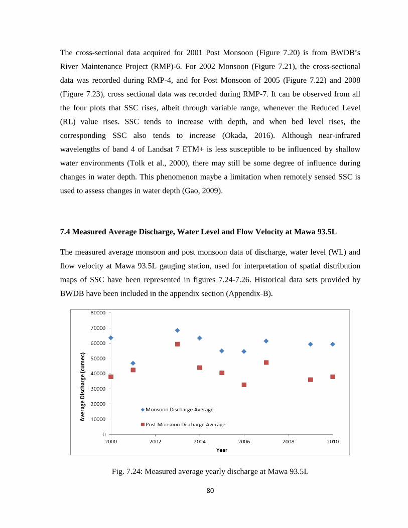
7.4 Measured Average Discharge, Water Level and Flow Velocity
7.6 Relationship between Measured SSC and Flow Velocity
Chapter 8. Conclusions and Recommendations
8.1 Conclusions
8.2 Recommendations
57
59
77
77
82
84
85
85
86
References
Appendix-A: Historical sediment data corresponding to Mawa SW 93.5L Appendix-B: Water Level, discharge and flow velocity data sets Appendix-C: DN values extracted from Landsat ETM+ images Appendix-D: Earth-sun distance correction coefficient (d) table
Appendix-E: Values of Eoλ, the mean solar ToA Irradiance
Appendix-F: List of all Landsat ETM+ images acquired for this thesis
87
95
102
108
117
121
122
ix
Page 10
List of Figures
Figure No. Page No.
Figure 2.1 Effect of SSC on the reflectance of red light tested in
laboratory
6
Figure 2.2 Correlation between ground-measured turbidity and satellite-
observed red reflectance
8
Figure 2.3 Scatterplots showing the natural logarithm (ln) of in situ SSC
measurements and red reflectance (band 2) and total
reflectance (band 1 + band 2 + band 3)
9
Figure 2.4 Suspended Matter (TSM) concentration as a function of
atmospherically corrected MODIS Terra 250 m band 1
reflectance
10
Figure 2.5 Plot of the concentrations of suspended sediments with base
pixel values for Landsat Multispectral Scanner (MSS) Band
1 data
11
Figure 2.6 Plot of the concentrations of suspended sediments with base
pixel values for Landsat Multispectral Scanner (MSS) Band
2 data
12
Figure 2.7 Plot of the concentrations of suspended sediments with base
pixel values for Landsat Multispectral Scanner (MSS) Band
3 data
12
Figure 2.8 Plot of the concentrations of suspended sediments with base
pixel values for Landsat Multispectral Scanner (MSS) Band
4 data
13
Figure 2.9 Graph of MSS radiance in band 5 plotted against suspended
solids
14
Figure 2.10 Distribution of TSS over the study area in Istanbul on 04
June 2005
15
Figure 2.11 Relation between SSC and water reflectance at Bands 1–4 in 17
x
Page 11
the Upper and Middle Yangtze River
Figure 2.12 SSC distribution map in the Upper Yangtze showing the
spatial variations of SSC
17
Figure 2.13 SSC distribution map in the Middle Yangtze showing the
spatial variations of SSC
18
Figure 2.14 SSC distribution map in the Lower Yangtze showing the
spatial variations of SSC
18
Figure 2.15 Regression relationship between SSC and water reflectance
between band 2 and band 5
19
Figure 2.16 Scatter plot of observed SSC against estimated SSC of the
Lower Yangtze River
20
Figure 2.17 Residual of SSC versus estimated SSC 20
Figure 2.18 Scatter plots and best-fit curves for the relationship between
SSL and Exoatmospheric reflectance
21
Figure 2.19 Scatter plot of predicted values by the polynomial model
based on NIR band Exoatmospheric reflectance and
measured values of SSL with 1:1 fit line
22
Figure 2.20 Relationship between reflectance of TM band 3 and
suspended sediment concentration (SSC) for Ganges-
Brahmaputra Rivers
23
Figure 3.1 Geologic map of the Bengal basin 26
Figure 3.2
Figure 3.3
Predicted sediment budget of the GBM delta
River channel patterns and typical cross-sections
27
29
Figure 3.4 Geomorphic map of the Bengal basin and surroundings
superimposed on the SRTM-90 m digital elevation model
30
Figure 3.5 Location of in situ data collection point 31
Figure 4.1 Bangladesh Water Development Board’s water survey
catamaran stationed at Mawa 93.5L gauge station
32
Figure 4.2 An automatic pulley system used to lift and submerge
gauging equipment
33
Figure 4.3 Sediment gauging equipment being prepared for sample 33
xi
Page 12
collection
Figure 4.4 Sediment sampling equipment being lowered for water
sample collection
34
Figure 4.5 Sediment sampling equipment being lifted up after water
sample collection
34
Figure 4.6 Water sample being transferred to another container from
sediment sampling equipment
35
Figure 4.7 Sample being transferred from the container to the
measurement tube using a funnel
35
Figure 4.8 Measurement tubes being separated after collection of
sample
36
Figure 4.9 Samples in measurement tubes being stored to be transferred
to laboratory for testing
36
Figure 4.10 Example of True Color Landsat 7 ETM+ Product 39
Figure 5.1 Screenshot of ILWIS while extraction of DN with pixel
information
41
Figure 6.1 Scatter plot of Measured SSC versus Reflectance Percentage
of Band 1
45
Figure 6.2 Scatter plot of Measured SSC versus Reflectance Percentage
of Band 2
46
Figure 6.3 Scatter plot of Measured SSC versus Reflectance Percentage
of Band 3
46
Figure 6.4
Figure 6.5
Figure 6.6
Figure 6.7
Scatter plot of Measured SSC versus Reflectance Percentage
of Band 4
Scatter plot of measured SSC versus ToA reflectance
percentage of bands 1-4 with linear trend lines
Scatter plot of measured SSC versus ToA reflectance
percentage of bands 1-4 with exponential trend lines
Scatter plot of measured SSC versus ToA reflectance
percentage of bands 1-4 with logarithmic trend lines
47
48
49
50
xii
Page 13
Figure 6.8 Scatter plot of estimated SSC values by the polynomial
model based on band 4 (Near Infrared) Exoatmospheric
reflectance and measured SSC data with 1:1 fit line.
51
Figure 6.9 Residue of SSC versus measured SSC 52
Figure 6.10 Scatter plot of relative error percentage of estimated SSC
from measured SSC
52
Figure 6.11 Bands 1-4 ToA reflectance percentage Plot 55
Figure 7.1 Spatial distribution map of SSC in the Padma River for
Monsoon of 2000
59
Figure 7.2 Spatial distribution map of SSC in the Padma River for Post-
Monsoon of 2000
60
Figure 7.3 Spatial distribution map of SSC in the Padma River for
Monsoon of 2001
61
Figure 7.4 Spatial distribution map of SSC in the Padma River for Post
Monsoon of 2001
62
Figure 7.5 Spatial distribution map of SSC in the Padma River for
Monsoon of 2002
63
Figure 7.6 Spatial distribution map of SSC in the Padma River for Post
Monsoon of 2002
64
Figure 7.7 Spatial distribution map of SSC in the Padma River for Post
Monsoon of 2003
65
Figure 7.8 Spatial distribution map of SSC in the Padma River for
Monsoon of 2004
66
Figure 7.9 Spatial distribution map of SSC in the Padma River for Post
Monsoon of 2004
67
Figure 7.10 Spatial distribution map of SSC in the Padma River for
Monsoon of 2005
68
Figure 7.11 Spatial distribution map of SSC in the Padma River for Post
Monsoon of 2005
69
Figure 7.12 Spatial distribution map of SSC in the Padma River for Post
Monsoon of 2006
70
xiii
Page 14
Figure 7.13 Spatial distribution map of SSC in the Padma River for
Monsoon of 2007
71
Figure 7.14 Spatial distribution map of SSC in the Padma River for Post
Monsoon of 2007
72
Figure 7.15 Spatial distribution map of SSC in the Padma River for
Monsoon of 2008
73
Figure 7.16 Spatial distribution map of SSC in the Padma River for Post
Monsoon of 2008
74
Figure 7.17 Spatial distribution map of SSC in the Padma River for Post
Monsoon of 2009
75
Figure 7.18
Figure 7.19
Spatial distribution map of SSC in the Padma River for Post
Monsoon of 2010
Temporal variation of SSC
76
77
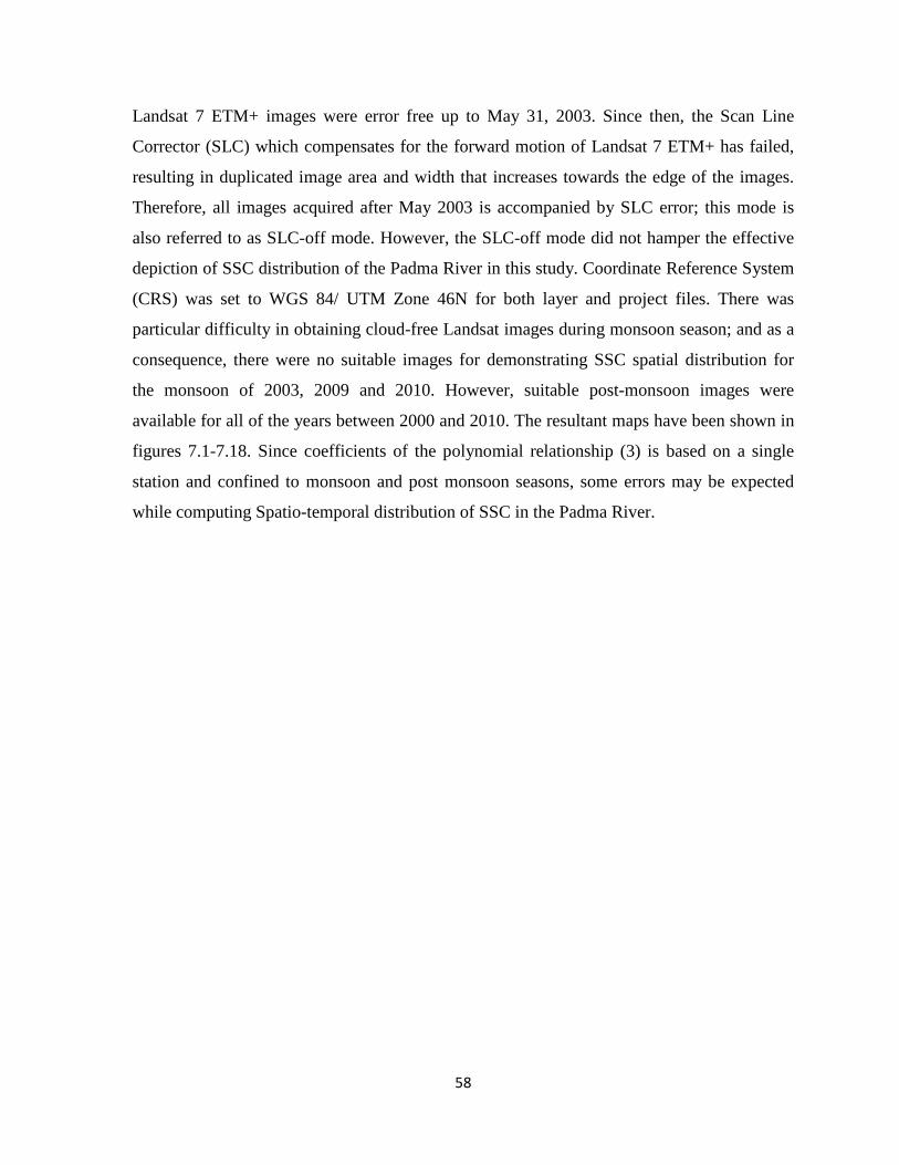
Figure 7.20 Variation of cross section and corresponding SSC for Post
Monsoon of 2001
78
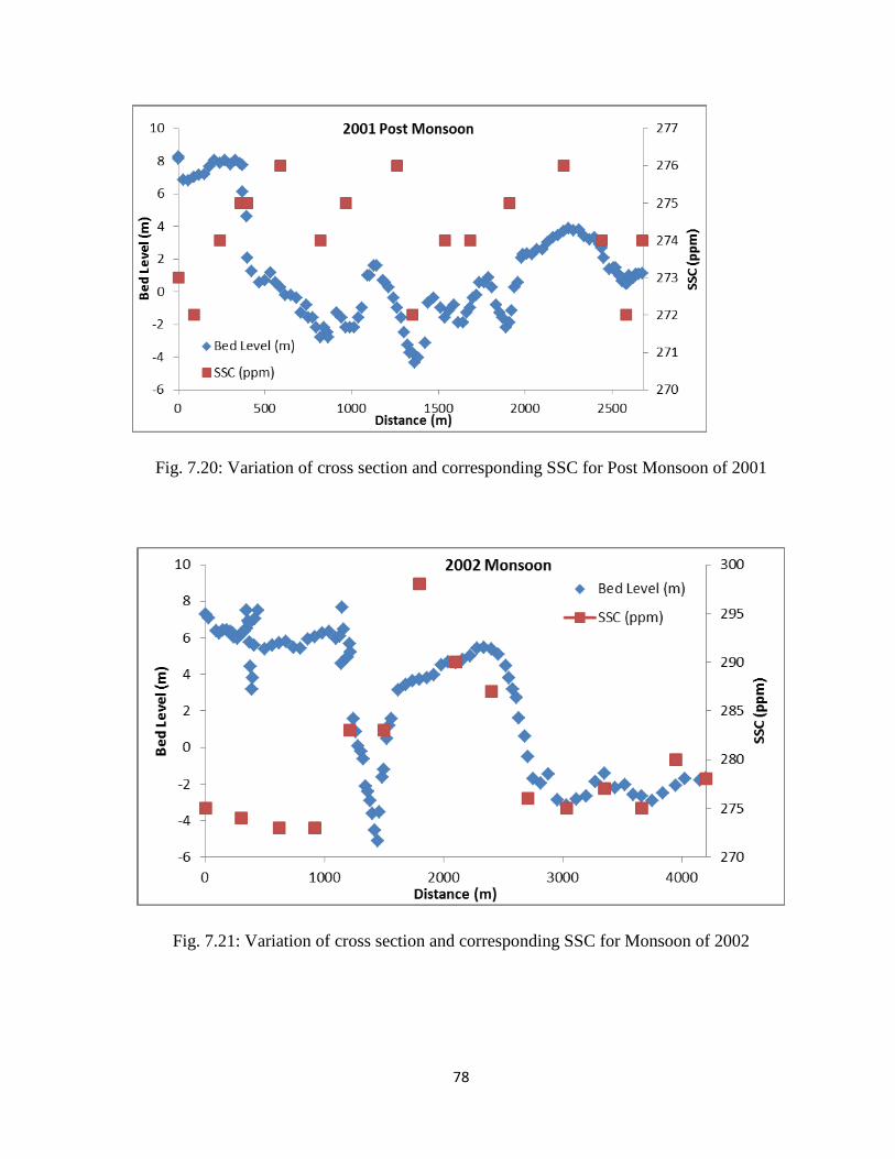
Figure 7.21 Variation of cross section and corresponding SSC for
Monsoon of 2002
78
Figure 7.22 Variation of cross section and corresponding SSC for Post
Monsoon of 2005
79
Figure 7.23 Variation of cross section and corresponding SSC for Post
Monsoon of 2008
79
Figure 7.24 Measured average yearly discharge at Mawa 93.5L 80
Figure 7.25 Measured average yearly water level at Mawa 93.5L 81
Figure 7.26 Measured average yearly flow velocity at Mawa 93.5L 81
Figure 7.27 Scatter plot of measured flow velocity and measured SSC 82
Figure 7.28 Spatial variation of flow velocity for monsoon of year 2000 84
Figure 7.29 Spatial variation of flow velocity for post monsoon of year
2002
84
xiv
Page 15
List of Tables
Table No. Page No.
Table 4.1 An example of the Padma’s sediment data set provided by the
BWDB
37
Table 5.1 Resultant ToA Reflectance (dimensionless) values 44
Table 6.1 Data sets used for validation of polynomial model 51
Table 6.2 Output table of regression analyses 54
Table 6.3 Summary of outputs of regression analyses 54
Table 6.4 Residual output of regression analyses 54
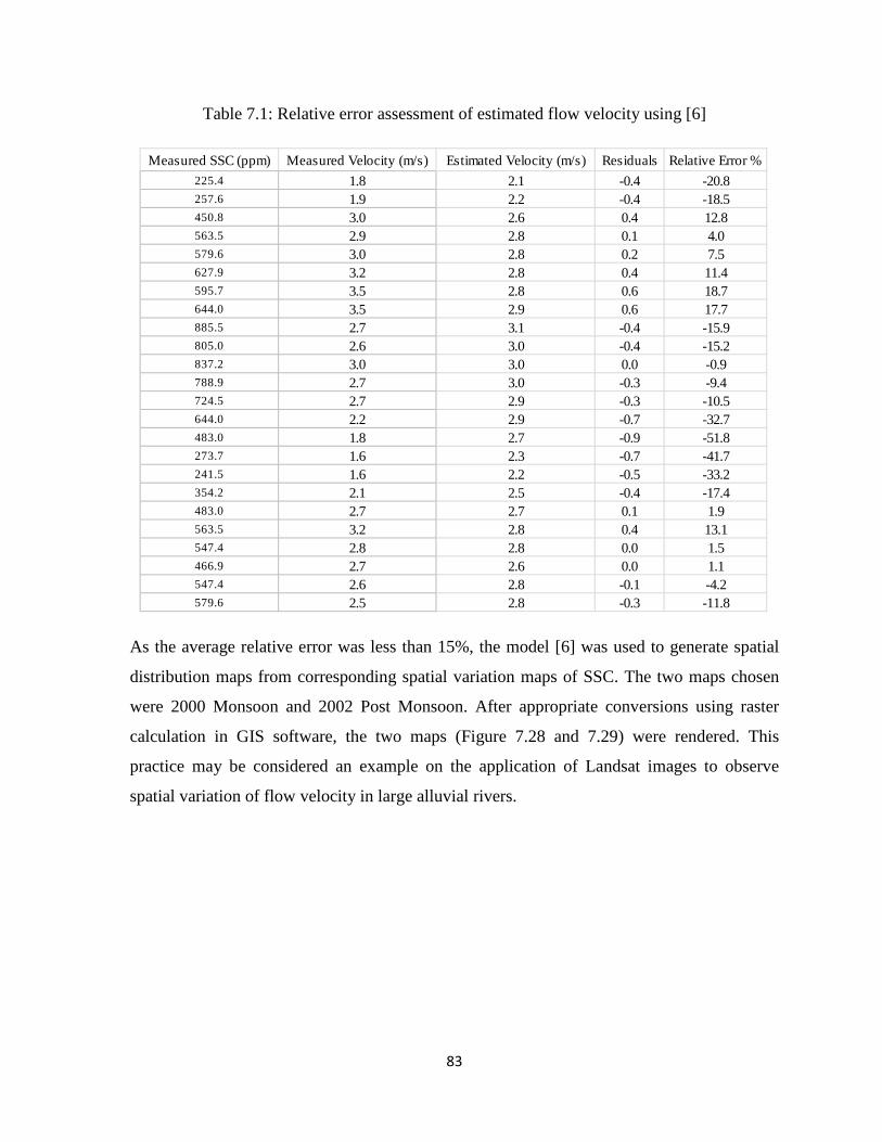
Table 7.1 Relative error assessment of estimated flow velocity 83
xv
Page 16
Abbreviations
IWFM Institute of Water and Flood Management
BWDB Bangladesh Water Development Board
BUET
NASA
USGS
EROS
TM
ETM+
MSS
MODIS
CMODIS
GBM
MRD
LP
PAD
SSC
AVHRR
SWIR
TSM
PPM
ARE
RMSE
RRMSE
ToA
BCM
WL
SSL
GPS
MSCD
Bangladesh University of Engineering and Technology
National Aeronautics and Space Administration
United States Geological Survey
Earth Resources Observation and Science
Thematic Mapper
Enhanced Thematic Mapper +
Multi Spectral Scanner
Moderate Resolution Imaging Spectroradiometer
Chinese Moderate Resolution Imaging Spectrometer
Ganges-Brahmaputra-Meghna
Mississippi River Delta
Lake Pontchartrain
Peace Athabasca Delta
Suspended Sediment Concentration
Advanced Very High Resolution Radiometer
Short Wave Infrared
Total Solid Matter
Parts Per Million
Absolute Relative Error
Root Mean Square Error
Relative Root Mean Square Error
Top of Atmosphere
Billion Cubic Meters
Water Level
Suspended Sediment Load
Global Positioning System
Mirror Scan Correction Data
xvi
Page 17
SLC
ILWIS
DN
TIF
QGIS
PToA%
Scan Line Corrector
Integrated Land and Water Information System
Digital Number
Tagged Image File
Quantum Geographic Information System
Top of Atmosphere Reflectance Percentage
xvii
Page 18
List of Symbols
Lλ = Spectral Radiance (m W cm-2 sr-1 μm-1)
Lmax = Radiance measured at detector saturation (m W cm-2 sr-1 μm-1)
Lmin
pλ
d
Eoλ
θs
= Lowest radiance measured by the sensor (m W cm-2 sr-1 μm-1)
= ToA or Exoatmospheric Reflectance as a function of the band width λ
= Correction factor for variation in solar irradiances due to varying earth-sun
distance
= Exoatmospheric Irradiance (Wμm-2)
= Solar Zenith Angle (rad)
Q
= Flow discharge (m3/s or cumec)
xviii
Page 19
Chapter 1 Introduction
1.1 Significance of Suspended Sediment Concentration
Suspended Sediment Concentration (SSC) is a measure of the amount of sediment suspended
in water bodies. The quantification of suspended sediments and their transport mechanism
are essential in understanding riverine, estuarine and coastal processes. SSC is required to
estimate and predict soil erosion and sediment transport caused by changes in land use
patterns (Collins and Walling, 2004). Suspended sediments also play important role in water
quality management because it is connected to total primary productivity, such as transport of
nutrients, to fluxes of metals, radio-nuclides and organic micro-pollutants (Ouillon et al.,
2004). Variations in SSC of rivers impact changes in river morphology. Alluvial river
channels are also classified with respect to the total sediment load delivered to the channel.
An excess of total load causes deposition, a deficiency causes erosion, and between the
extremes lays the stable channel. Moreover, suspended sediment is a dominant factor in the
Ganges and Brahmaputra Rivers. For Brahmaputra, the ratio of the bedload discharge to the
suspended sediment discharge was 10-25(Okada, 2016). SSC is also an indicator of river
planform. It is important to accurately monitor and archive synoptic SSC data of rivers to
understand and track changes in river morphology and water quality.
Suspended sediments are significant for sustaining complex river ecosystems and aquatic
life. Many human activities in or near aquatic habitats re suspend bottom sediments and
create turbid conditions that differ in scope, timing, duration, and intensity from the
resuspension events induced by storms, freshets, or tidal flows. Dredging of navigation
channels is one such source of bottom disturbance. Suspended sediments can elicit a variety
of responses from aquatic biota, primarily because many attributes of the physical
environment are affected. Physical impacts from increased concentrations of suspended
sediment on aquatic life can be detrimental, for example, resulting in egg abrasion, reduced
bivalve pumping rates, and direct mortality (Wilber and Clarke, 2001). However some
species of fishes in alluvial rivers thrive in turbid and sediment rich conditions. Previous
1
Page 20
studies reveal that several species actively prefer turbid over clear water conditions; using
turbid conditions to facilitate feeding and avoidance behaviors (Cyrus and Blaber, 1987).
Also sediments provide essential nutrients for unique local ecosystem to survive and flourish.
1.2 Constraints in Acquisition of SSC Data
The task of obtaining and reliable and constant spatio-temporal SSC data of rivers in
Bangladesh is severely limited. These limitations include size and extent of rivers, financial
and economic constraints; lack of experienced personnel. Although in situ measurement
techniques of suspended sediment are continually changing, it is generally accepted that they
do not completely satisfy requirements. Instruments used traditionally to evaluate SSC have
been limited to single location, and therefore variations in SSC have been obtained by
profiling or by using a fixed vertical array of measuring devices. Mechanical measurement
techniques are both time consuming and have poor temporal resolution. There are additional
problems with regard to logistics; problems in deployment and calibration of
devices. Acoustic Doppler profilers using acoustic backscatter to measure suspended
sediment concentrations in orders of magnitude are being used widely recently (Gray and
Gartner, 2009). The technology is relatively robust and generally immune to effects of
biological fouling. However, these devices have constraints in terms of spatial coverage.
Conventional techniques are often constrained in their capability to provide comprehensive
spatial and temporal data of SSC (Crawford and Hay, 1993; Sheng and Hay, 1988; Thorne
and Hardcastle, 1997; Thorne et al., 1993).
1.3 Significance of SSC in the Ganges-Brahmaputra Rivers
The Ganges-Brahmaputra Rivers System carries the world’s highest yearly sediment loads of
approximately one billion tons (Milliman and Meade, 1983; Milliman and Syvitski, 1992b).
Due to the large size and extent of these rivers, study of sediments and their spatial-temporal
characteristics in the delta has been restricted (Rice, 2007). Approximately 33% of the annual
sediment load is deposited in the river flood-plain (Goodbred Jr and Kuehl, 1998; Goodbred
2
Page 21
and Kuehl, 1999), 21% is deposited in the beds of the subaqueous delta (Michels et al.,
2003), 20% contributes to subaqueous delta progradation in the foreset beds, and 25% is
conveyed to the Swatch of No Ground Canyon (Goodbred and Kuehl, 1999). 1-2% of the
annual sediment load contributes to the prograding subaerial delta (Allison, 1998).
Suspended Sediment Concentration is therefore a very useful parameter in the study of
alluvial rivers such has Ganges, Brahmaputra and Meghna. Reliable historical SSC data is
required to observe and predict aggradation and degradation of river beds, erosion and
accretion of river banks, and to carry out various hydro-morphological analysis.
1.4 Remote Sensing using Landsat
From 1972, Landsat satellites have consistently acquired space-based images of the Earth’s
land surface, coastal shallows, and coral reefs. Open-access Landsat data are being utilized
by government, commercial, industrial, civilian, military, and educational communities
throughout the world. These data support a plethora of applications in areas such as global
change research, studies on water bodies, agriculture, forestry, geology, resource
management, geography, mapping, water quality, and coastal studies. Landsat satellites
acquire images of the Earth’s surface along the satellite’s ground track in a 185-kilometer-
wide swath as the satellite moves in a descending orbit over the sunlit side of the Earth.
Landsat 7 orbits the Earth at an altitude of 705 kilometers. It completes orbit every 99
minutes, 14 full orbits per day, and covers every geographic point on Earth once every 16
days. Although each satellite has a 16-day temporal resolution, their orbits allow 8-day repeat
coverage of any Landsat scene area on the globe. Landsat 7 carries the Enhanced Thematic
Mapper Plus (ETM+), with 30-meter visible, near-IR, and SWIR bands, a 60-meter thermal
band, and a 15-meter panchromatic band (USGS, 2013). Satellite remote sensing offers a
feasible alternative option of acquiring SSC data over large spatial extent and high temporal
repeatability.
3
Page 22
1.5 Scope of the Study
The Padma River starts downstream from the point where the Ganges and Brahmaputra
Rivers confluence. In this thesis, satellite remote sensing of SSC in the Padma River was
focused upon. Multiple Landsat ETM+ images were processed; cloud-free Landsat-7 ETM+
images of both monsoon and post monsoon seasons, extending between 2000 and 2010 were
used in this study. Rarity of Landsat images during monsoon season was a notable aspect.
Multiple regression and correlation analyses were applied in this study. Open source GIS
software was used to generate spatial distribution maps. Scatter plots and their respective
coefficient of determination were used at multiple stages of this study.
1.6 Objectives of the Study
i. To establish a correlation between suspended sediment concentrations and spectral
reflectance of the Padma River and to use that correlation to estimate its historical
suspended sediment concentrations.
ii. To investigate the relationships between SSC levels and corresponding spatio-
temporal variations in the channel hydro-morphology of the Padma River.
4
Page 23
Chapter 2
Literature Review
2.1 Application of Remote Sensing in Retrieval and Monitoring of SSC Values
Since Landsat images became available in 1972, they have been used for monitoring of
inland and coastal water bodies, including retrieval of quantitative data concerning the water
area. One of the earliest studies showed that quantitative estimates of suspended sediment
concentration of surface water could be made using reflected solar radiation (Ritchie et al.,
1976). Another one of the earliest studies developed a model for obtaining volume spectral
reflectance from the surface radiance of a water body, and spectrometer data, showing that
multispectral algorithms exist which can relate volume spectral reflectance to either
nonfilterable residue or nephelometric turbidity with accuracy, and turbidity had emerged as
the best suited for measurement by remote sensing techniques for reasons of accuracy and
signature transferability (Holyer, 1978).
Turbidity can be quantified directly using a light turbidimeter, or visually using Secchi disc
depth. Because sediment concentration is often the primary control on turbidity, the two
quantities are frequently treated similarly with respect to remote sensing (Ritchie et al.,
2003). In 1988, a study suggested that SSC-Spectral Reflectance relationship is difficult to
both quantify and utilize. It is difficult to quantify because of the many environmental factors
that disturb the relationship. These include the atmosphere, sensing geometry,
water/atmosphere boundary, water components and concentration of suspended sediments. It
is difficult to utilise because of the problems associated with sampling the SSC that is
necessary to both train and test any estimation procedure (Curran and Novo, 1988). Figure
2.1 shows the results of a 1972 laboratory study (Scherz, 1972) on the effect of SSC on the
reflectance of red light, and was one of the first to demonstrate the non-linear relationship
between spectral reflectance and SSC. Spectral reflectance is not linearly related to SSC; it is
5
Page 24
controlled by many factors including the sediment properties such as size, mineralogy and
color (Rimmer et al., 1987).
Fig. 2.1: Effect of SSC on the reflectance of red light tested in laboratory (Scherz, 1972)
2.2 Constraints in the Estimation of SSC from Spectral Reflectance
The estimation of SSC from remotely sensed spectral reflectance has followed all or, more
usually some of the generic five stages mentioned below (Curran, 1987; Tassan, 1987).
i. Simultaneous measurement of SSC and spectral reflectance.
ii. Correct, as far as possible, for environmental influences on (i).
iii. Derive an empirical relationship between corrected SSC and spectral reflectance on a
training set of data.
iv. Use corrected spectral reflectance and the relationship in (iii) to estimate SSC.
v. Determine the accuracy of SSC estimation using a testing set of corrected SSC data.
However, majority of the studies terminated at stage (iii) on the assumption that a statistically
significant correlation between SSC and spectral reflectance is the foundation for accurate
estimation.
6
Page 25
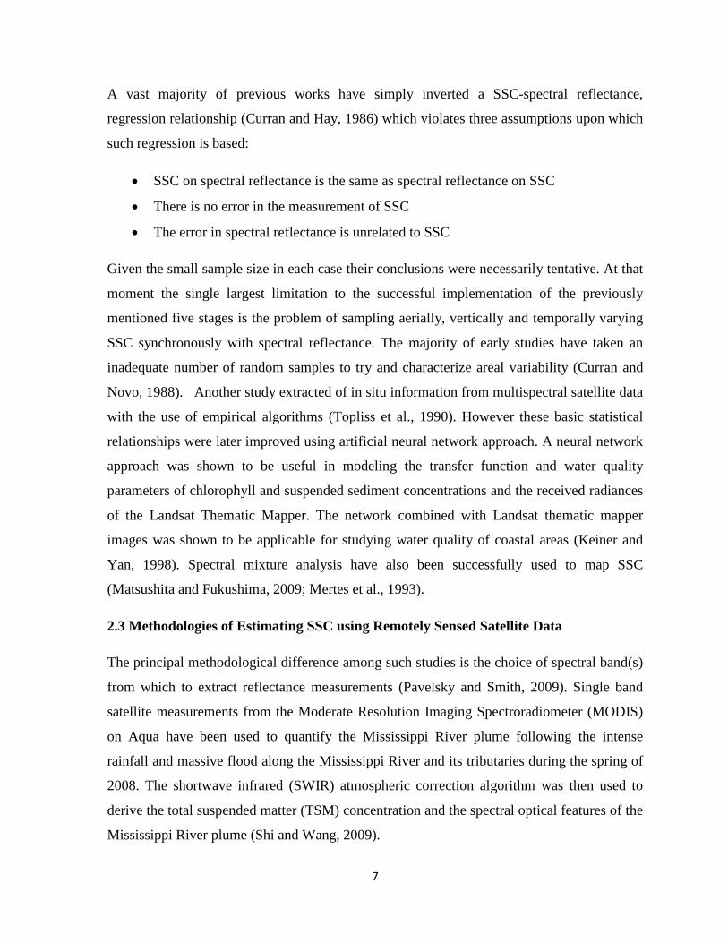
A vast majority of previous works have simply inverted a SSC-spectral reflectance,
regression relationship (Curran and Hay, 1986) which violates three assumptions upon which
such regression is based:
• SSC on spectral reflectance is the same as spectral reflectance on SSC
• There is no error in the measurement of SSC
• The error in spectral reflectance is unrelated to SSC
Given the small sample size in each case their conclusions were necessarily tentative. At that
moment the single largest limitation to the successful implementation of the previously
mentioned five stages is the problem of sampling aerially, vertically and temporally varying
SSC synchronously with spectral reflectance. The majority of early studies have taken an
inadequate number of random samples to try and characterize areal variability (Curran and
Novo, 1988). Another study extracted of in situ information from multispectral satellite data
with the use of empirical algorithms (Topliss et al., 1990). However these basic statistical
relationships were later improved using artificial neural network approach. A neural network
approach was shown to be useful in modeling the transfer function and water quality
parameters of chlorophyll and suspended sediment concentrations and the received radiances
of the Landsat Thematic Mapper. The network combined with Landsat thematic mapper
images was shown to be applicable for studying water quality of coastal areas (Keiner and
Yan, 1998). Spectral mixture analysis have also been successfully used to map SSC
(Matsushita and Fukushima, 2009; Mertes et al., 1993).
2.3 Methodologies of Estimating SSC using Remotely Sensed Satellite Data
The principal methodological difference among such studies is the choice of spectral band(s)
from which to extract reflectance measurements (Pavelsky and Smith, 2009). Single band
satellite measurements from the Moderate Resolution Imaging Spectroradiometer (MODIS)
on Aqua have been used to quantify the Mississippi River plume following the intense
rainfall and massive flood along the Mississippi River and its tributaries during the spring of
2008. The shortwave infrared (SWIR) atmospheric correction algorithm was then used to
derive the total suspended matter (TSM) concentration and the spectral optical features of the
Mississippi River plume (Shi and Wang, 2009).
7
Page 26
Single band of IKONOS satellite, as shown in Figure 2.2, was shown to have positive
correlation with ground measured turbidity in the lower Charles River in Boston, United
States of America, which demonstrated the usability of high-resolution satellite data for
mapping turbidity in the lower Charles River (Hellweger et al., 2007).
Fig. 2.2: Correlation between ground-measured turbidity and satellite-observed red
reflectance (Hellweger et al., 2007)
AVHRR satellite imagery have been used to monitor in situ water quality data; multiple in
situ water quality data and reflectance were used to calibrate a general optical equation
(Woodruff et al., 1999). Some studies have also conflated red reflectance with reflectance in
one or multiple other visible bands to create robust relationships, especially in the case of
varying sediment color. Data from the Chinese Moderate Resolution Imaging
Spectroradiometer (CMODIS), loaded on the China’s SZ-3 spacecraft, have been used for
concentration retrieval of the suspended sediment. Using an empirical line method, the
CMODIS radiance was converted to the water-leaving reflectance, and is applied to inversion
of the suspended sediment concentrations in the Yangtze River estuary. The concentrations
ranging between 0 mg/L and 1000 mg/L are well validated by the field measurement data
(Han et al., 2006).
8
Page 27
The use of a near infrared band for Total Suspended Matter (TSM) retrieval in surface waters
has been suggested (Ritchie et al., 1976). Near Infrared bands have the least impacts from
chlorophyll and colored dissolved organic carbon. Furthermore, shorter wavelengths
integrate over a larger water column while penetration depth at 833 nm is small (much less
than 1 m in turbid waters). The latter corresponds to the depth of the in situ water sampling.
Although single-bands reflectance in the near-IR (746, 774, 803, 833, or 862 nm) performed
well for the shipborne reflectance (Sterckx et al., 2007). The use of total reflectance
combining bands 1, 2 and 3 of ASTER and SPOT images seemed to generate stronger
statistical relationship compared to only red band (Figure 2.3). To assess detailed spatial
patterns in SSC in the Peace Athabasca Delta (PAD), Canada, robust positive relationships
between in situ suspended sediment concentration (SSC) and remotely sensed visible/near-
infrared reflectance for four days in 2006 and 2007 were applied, revealing strong variations
in water sources and flow patterns, including flow reversals in major distributaries (Pavelsky
and Smith, 2009).
Fig. 2.3: Scatterplots showing the natural logarithm (ln) of in situ SSC measurements and red
9
Page 28
reflectance (band 2) and total reflectance (band 1 + band 2 + band 3) from one high
resolution SPOT image acquired on June 15, 2007 and two ASTER images acquired on July
19, 2006 and July 13, 2007. In each case, the use of total reflectance rather than red
reflectance results in a stronger statistical correlation indicated by the higher r2. Points are
colored according to region. In the case of total reflectance, results suggest that mean
divergence from the overall regression line does not differ by region (Pavelsky and Smith,
2009)
Multiple studies have demonstrated that water reflectance in the NIR and visible spectral
regions (bands 1-4) of Landsat images correlate quite strongly with SSC (Ritchie and
Schiebe, 2000). Therefore, reflectance is usable as an indicator of SSC for inland and coastal
waters. One study demonstrated that the characteristics of the MODIS Terra instrument
provide data well suited for the study of suspended matter in dynamic coastal waters (Figure
2.4). The moderately high resolution of MODIS 250 m data was useful for mapping small-
scale features of TSM concentration in different inland and coastal waters (Miller and
McKee, 2004).
Fig. 2.4: Suspended Matter (TSM) concentration as a function of atmospherically corrected
MODIS Terra 250 m band 1 reflectance. TSM data were obtained from six field campaigns:
Mississippi Sound, 5/16/2001 (o); Mississippi River Delta (MRD), 3/17/02 (•); Lake
10
Page 29
Pontchartrain (LP), 5/19/02 (■); LP, 5/23/02 (D); MRD, 7/15/03 (▲); and MRD, 10/20/03
(□). The line is the least-squares fit to the data (Miller and McKee, 2004).
Previous studies have also shown water bodies with higher turbidity demonstrate much
stronger scattering compared to waters with lower turbidity (Kirk, 1994). Digital Numbers
(DN)s have been directly used in past studies to retrieve SSC values from water using
satellite remote sensing. Digital spectral data from 14 Landsat MSS scenes of Moon Lake in
Coahoma County, Mississippi were analyzed and compared with ground measurements of
total solids and suspended sediments in the lake surface water for the period between January
1983 and May 1985. Coefficients of determination of greater than 0.81 were calculated
between MSS Band 2 (0.6-0.7 µm) or Band 3 (0.7-0.8 µm) and suspended sediments or total
solids. Coefficients of determination for multiple regression (Figures 2.5-2.9) using three or
four MSS bands were greater than 0.90 (Ritchie et al., 1987).
Fig. 2.5: Plot of the concentrations of suspended sediments with base pixel values for
Landsat Multispectral Scanner (MSS) Band 1 data (Ritchie et al., 1987)
11
Page 30
Fig. 2.6: Plot of the concentrations of suspended sediments with base pixel values for
Landsat Multispectral Scanner (MSS) Band 2 data (Ritchie et al., 1987)
Fig. 2.7: Plot of the concentrations of suspended sediments with base pixel values for
Landsat Multispectral Scanner (MSS) Band 3 data (Ritchie et al., 1987)
12
Page 31
Fig. 2.8: Plot of the concentrations of suspended sediments with base pixel values for
Landsat Multispectral Scanner (MSS) Band 4 data (Ritchie et al., 1987)
Physically quantified values of spectral radiance, which is converted from DN through in-
flight calibration sensor parameters, have also been used to indicate SSC values for coastal
waters. Digital data from Landsat's Multiple Spectral Scanners (MSS) were used to calculate
the amount of radiation received from sea level at the position of the satellite. After assessing
the atmospheric effects, on the radiance data, the amount of radiance was then related to
sediment concentration (Aranuvachapun and LeBlond, 1981). An earlier study had also
applied a single band of MSS data to investigate correlation between radiance and suspended
sediments or suspended solids (Figure 2.8).
13
Page 32
Fig. 2.9: Graph of MSS radiance in band 5 plotted against suspended solids (Munday and
Alföldi, 1979)
However reflectance values, especially exo-atmospheric or top of atmosphere reflectance
have been the most widely used for indicating SSC; for example, Band 3 (Red) of SPOT-
XS2 demonstrated strong correlation with SSC within a range of 0-10 ppm. Similarly,
MODIS Terra Band 1 showed significant correlation with SSC range of 0-60 ppm.
Reflectance in the Band 2 and Band 4 of Landsat ETM+ have been used in the past to
retrieve SSC values (Ouillon et al., 2004). Reduction of the influence of particle grain size
and refractive index variation was shown to be possible through use of reflectance ratio. Also
reflectance ratios of specific spectral regions demonstrated quite good correlation with SSC
(Doxaran et al., 2002). Information from the Landsat 5 (TM sensor), Landsat 7 (ETM sensor)
and SAC-C (MMRS sensor) satellites have been used in combination with on-site
measurements to study the spatial and temporal characteristics of permanent lakes in the
Ibera macrosystem in Argentina (Cózar et al., 2005).
14
Page 33
High Resolution Ikonos Multispectral Imagery have been used to retrieve Total Suspended
Solids (TSS) in a study conducted on Istanbul, Turkey (Ekercin, 2007). Multi regression of
dependent variable TSS study showed that all spectral bands contribute to the variance in
TSS. Therefore, all spectral bands were used to develop a final model to predict TSS Blue,
and NIR bands have negative, green and red bands have positive relationship with TSS. All
bands significantly contributed 97.24% of the variance in TSS. The model was then used to
generate spatial variation map of the study area (Figure 2.9).
Fig. 2.10: Distribution of TSS over the study area in Istanbul on 04 June 2005. The base
image is 04/06/2005 dated IKONOS Pan data (Ekercin, 2007)
15
Page 34
Algorithms to define the relationship between in situ SSC and corresponding spectral
radiance or reflectance have been developed to indicate SSC directly using satellite images
(Pavelsky and Smith, 2009; Reddy and Srinivasulu, 1994; Xia, 1993). Most of these studies
investigated relations for water bodies such as lakes, reservoirs and coastal regions; mainly
waters with very low to moderate turbidity. Also, many of their concentrations were on
water quality (Zhang et al., 2003) aspects rather than morphological aspects associated with
rivers, especially alluvial rivers.
2.4 Satellite Remote Sensing of SSC in Large Alluvial Rivers
In terms of rivers, very few studies have been undertaken regarding satellite remote sensing
of parameters such as SSC. Even fewer studies have concentrated on the relationship
between remotely sensed SSC and characteristics of alluvial rivers, such as cross section,
discharge, flow velocity and water levels. Especially highly turbid large rivers have been
largely ignored when it comes to the remote sensing of suspended sediments. A study
concerning Yangtze River in China used multi-temporal Landsat ETM+ to estimate its SSC
(Wang et al., 2009). Using an effective easy-to-use atmospheric correction method that does
not require in situ atmospheric conditions, retrieved water reflectance of Band 4 was found to
be a good SSC indicator within the large SSC range 22–2610 mg /1 (Figure 2.11). The
regression relation between SSC and water reflectance of Band 4 appeared to be able to
provide a relatively accurate SSC estimate directly from Landsat ETM+ images for the
Yangtze River from the upper, the middle to the lower reaches. Using the regression relation,
SSC spatial maps were generated for upper, middle and lower Yangtze River (Figure 2.12-
2.14)
16
Page 35
Fig. 2.11: Relation between SSC and water reflectance at Bands 1–4 in the Upper and Middle
Yangtze River: (a) Band 1; (b) Band 2; (c) Band 3;(d) Band 4 (Wang et al., 2009)
Fig. 2.12: SSC distribution map (a) and enlarged part of it (b) in the Upper Yangtze showing
17
Page 36
the spatial variations of SSC. SSC values were retrieved directly from a Landsat ETM+
image (Wang et al., 2009)
Fig. 2.13: SSC distribution map (a) and enlarged part of it (b) in the Middle Yangtze showing
the spatial variations of SSC values retrieved directly from a Landsat ETM+ image (Wang et
al., 2009)
Fig. 2.14: SSC distribution map (a) and enlarged part of it (b) in the Lower Yangtze showing
the spatial variations of SSC. SSC values were retrieved directly from a Landsat ETM+
image (Wang et al., 2009)
18
Page 37
Another study concerning large turbid river presented a method of estimating SSC of the
Yangtze at Jiujiang using time-series satellite data of high temporal resolution Terra MODIS
(Wang and Lu, 2010). It was found that differences in water reflectance between Band 2 and
Band 5 could provide relatively accurate SSC estimation even when in situ atmospheric
conditions were unknown (Figure 2.15). After validation (Figure 2.16-2.17), mean absolute
relative error (ARE) and relative root mean square error (RRMSE) were found to be
relatively low (i.e., 25.5% and 36.5%, respectively). This empirical relationship was
successfully applied to the estimation of SSC at Datong in the Lower Yangtze River,
although the SSC values were generally underestimated (Wang and Lu, 2010). This study
suggested that Terra MODIS could be used to estimate SSC in large turbid rivers, although
some influencing factors required further study to improve the accuracy of SSC estimation.
Fig. 2.15: Regression relationship between SSC and water reflectance between band 2 and
band 5 (Wang and Lu, 2010)
19
Page 38
Fig 2.16: Scatter plot of observed SSC against estimated SSC of the Lower Yangtze River
(n=33), where the line indicates a 1:1 relationship (Wang and Lu, 2010)
Fig 2.17: Residual of SSC versus estimated SSC (Wang and Lu, 2010)
20
Page 39
Another notable study studied the monitoring of suspended sediment load in the Mekong
River; the applicability for monitoring suspended sediment load (SSL) in the Mekong River
over temporal and spatial dimensions was investigated (Fleiflea, 2013). Landsat scenes
captured between 1988 and 2000, including 110 Thematic Mapper (TM) images and 21
Enhanced Thematic Mapper Plus (ETM+) images, were analyzed in correspondence with
ground observations. The three visible and near infrared bands were included in the analysis.
The polynomial relationship of the NIR Exoatmospheric reflectance, band 4 wave length:
760- 900 nm, to SSL based on the ground observations at 9 sites along the river demonstrated
the best agreements (overall R2, 0.76) (Figure 2.18-2.19). Subsequently, the equation enabled
reasonable estimation of the suspended sediment load longitudinal profiles and its temporal
changes. Thus, the results confirmed a high applicability of satellite image for monitoring
SSL in relatively large rivers such as the Mekong River (Fleiflea, 2013).
Fig 2.18: Scatter plots and best-fit curves for the relationship between SSL and
Exoatmospheric reflectance (a) band 1, R2=0.436; (b) band 2, R2=0.358; (c) band 3,
R2=0.566; (d) band 4, R2=0.76 (Fleiflea, 2013)
21
Page 40
Fig 2.19: Scatter plot of predicted values by the polynomial model based on NIR band
Exoatmospheric reflectance and measured values of SSL with 1:1 fit line (Fleiflea, 2013)
One study applied spectral mixture analysis to estimate the concentration of suspended
sediment in surface waters of the Amazon River wetlands from Landsat MSS and TM images
(Mertes et al., 1993). One study regarding the satellite remote sensing of suspended
sediments in Bangladesh is on the Ganges and Brahmaputra Rivers using older Landsat TM
and AVHRR data (Islam et al., 2001). Although this study made use of five data points to
develop relationship between suspended sediment and DN values directly, only three images
were used. A relationship between reflectance of TM band 3 and suspended sediment
concentration (SSC) was established during this study (Figure 2.20). Another similar study
(Islam et al., 2002)concentrated on the Distribution of suspended sediment in the coastal sea
off the Ganges–Brahmaputra River mouth. However, no comprehensive study regarding the
remote sensing of SSC in the Padma River has yet been published for the large alluvial
Padma River in Bangladesh.
22
Page 41
Fig 2.20: Relationship between reflectance of TM band 3 and suspended sediment
concentration (SSC) for Ganges-Brahmaputra Rivers (Islam et al., 2001)
23
Page 42
Chapter 3 - The Ganges-Brahmaputra Rivers System
3.1 Significance of Geographical Location
More than 2% of the world’s six billion population reside in the Bengal Basin, an area of
about 200,000 km2, covering most of Bangladesh and parts of eastern India, and is the
world’s largest fluvio-deltaic system (Alam et al., 2003; Coleman, 1976). The annual flow of
the Brahmaputra River from China to India is 165.4 billion cubic metres (BCM), from
Bhutan to India 78 BCM, and from India to Bangladesh 537.2 BCM (Rasul, 2015). The
annual flow of the Ganges River from China to Nepal is 12 BCM. All the rivers in Nepal
drain into the Ganges River; the annual flow from Nepal to India is 210.2 BCM. The annual
flow of the Ganges from India to Bangladesh is 525 BCM (Rasul, 2015). The major source of
water is the summer monsoon and snow and ice melt from the Himalayas. Water regimes are
strongly influenced by the monsoon. About 84% of the rainfall occurs from June to
September, and 80% of the annual river flow takes place in the four months from July to
October (Sood and Mathukumalli, 2011). The drastically reduced rainfall from November to
March has created a flood-drought syndrome in the basin. While huge amounts of water
during the monsoon period trigger floods and other hazards, the water in the dry season is
insufficient to meet the requirements for irrigation and navigation or to maintain the
minimum environmental flow in the rivers. Considerable areas in the Ganges-Brahmaputra
region often suffer from both floods and droughts, which cause huge economic and social
losses (Sood and Mathukumalli, 2011).
The Bengal basin also represents the world’s largest sediment dispersal system and has
formed the world’s biggest submarine fan, known as the Bengal fan (Kuehl et al., 1989).
River Ganges enters into the Bengal basin from the northwest after draining the Himalayas
and about 2500 km through India. The Ganges divides into two distributaries; the River
Padma flows southeast toward the confluence with the River Brahmaputra in Bangladesh
(Mukherjee et al., 2009). The Brahmaputra channel belt shows a rapid lateral migration of as
much as 800 m/year (Allison, 1998). Physiographically, the Bengal basin can be divided into
two major units, the Pleistocene uplands and Holocene sediments (Heroy et al., 2003).
24
Page 43
3.2 Geologic History of the Ganges-Brahmaputra Basin
The eastern part of the Bengal basin is mostly floored with Quaternary sediments deposited
by the Ganges, Brahmaputra and Meghna rivers and their numerous tributaries and
distributaries. The Ganges River rises near the Tibet-India border and flows southeast across
India into Bangladesh. Its drainage basin lies predominantly in highly weathered sediments
and volcanics, with the result that a heavy clay load is imposed on the channel. The
Brahmaputra River has its source within Tibet along the northern slope of the Himalayas and
flows across Assam into Bangladesh. This drainage basin contains very young and
unweathered sedimentary rocks, and little clay is available for transport. The bedload thus
consists predominantly of silt and fine sand. Of the two rivers, however, the Brahmaputra has
the slightly higher total sediment concentration. The sediments within the rivers of
Bangladesh, therefore, consist primarily of fine sands arid silts, with little clay matrix. Being
recently deposited, the sediments contain high water content and are loosely compacted. The
nature of these sediments and the great amount of material imposed on the channels by the
watershed causes the rivers constantly to adjust their bed configurations to differing flow
regimes. Thus the sediments of the Brahmaputra and Ganges rivers are not only deposited in
millions of tons but are also highly susceptible to erosion when flow conditions change.
Within Quaternary times both rivers have occupied and abandoned numerous distinct courses
(Coleman, 1969). Geologic map of the greater Bengal basin has been shown in Figure 3.1.
25
Page 44
Fig. 3.1: Geologic map of the Bengal basin (Heroy et al., 2003)
3.3 Nature of Sediment Transport along the Ganges-Brahmaputra Rivers
The Ganges-Brahmaputra River transports approximately 1 × 10⁹ tonnes of sediment per
year, ranking it highest in the world among the river systems (Milliman and Syvitski, 1992a).
An estimated 80% of this sediment load is delivered while southwest monsoon prevails from
June to September (Coleman, 1969), rendering the system especially vulnerable to regional-
scale climatic forcing. Approximately 8.5 × 10¹² m3 of Ganges-Brahmaputra sediment has
been stored in the Bengal basin since ca. 11 000 year before present (Goodbred and Kuehl,
2000). At the margin of the continent, the Ganges-Brahmaputra sediment load drains through
the Bengal basin. The Bengal basin consists of approximately 1 × 10⁵ km2 of flood-plains
and delta-plains. The Padma, like Ganges and Brahmaputra is a very dynamic river; amounts
26
Page 45
of deposition, accretion and lateral channel migration are very high. Fluvial sediment
delivery to the GBM delta is projected to increase under the influence of anthropogenic
climate change, albeit with the magnitude of the increase varying according to the specific
catchment being considered. By the middle part of the 21st century, sediment loads are
projected to increase by between 16% and 18% for the Ganges, and between 25% and 30%
for the Brahmaputra River (Darby et al., 2015). A representation of the sediment budget of
the GBM delta based on this study has been shown in Figure 3.2. The Padma River re-
arranges its channel every year and overbank inundation dispenses river's sediment load over
the delta. Alluvial sediments are necessary for regulating soil fertility in the GBM delta, but
this pattern is also detrimental to the lives and livelihoods of people. Over the last thirty
years, erosion has devoured hundreds of thousands hectares of arable land along the Ganges,
Brahmaputra and Padma banks. SSC is a major parameter in understanding and predicting
river evolution, and therefore of significance in Bangladesh.
Fig. 3.2: Predicted sediment budget of the GBM delta (Courtesy - ESPA Deltas Project)
27
Page 46
3.4 Morphology of the Ganges-Brahmaputra System
Most of the major rivers can generally be grouped into three types: braided, straight, and
meandering. The presence of only one alluvial island (braid or, locally in Bangladesh, char)
is sufficient to make the channel braided, but most braided rivers show several islands
between channel banks (Figure 3.3). The chars are a product of the river itself and are
composed of both bedload and suspended sediment. In plan view, the chars are
asymmetrically diamond-shaped or triangular, with one point of the triangle pointed
upstream. Although these two major shapes are most common, other types can be found.
Generally the islands are unstable and change their location frequently. However, under
certain conditions, such as stabilization by vegetation, they become semi-permanent. Since
most chars modify their size, shape and location from time to time, they cause drastic
changes in cross-sectional area at any one point. Brahmaputra can be classified as braided.
The detailed processes responsible for the formation of a braided river are still poorly
understood. Many published works deal specifically with the process of braiding, but little
agreement can be found, and the hydraulic parameters of a braided stream are extremely
complex (Coleman, 1969). Ganges is a sediment laden, wide, meandering river. It’s annual
mean predicted sediment load is 498.8 x 10⁶ tons (Islam and Jaman, 2006). A geomorphic
map of the Bengal basin has been shown in Figure 3.4.
28
Page 47
Fig 3.3: River channel patterns and typical cross-sections: A. braided; B. straight; C.
meandering (Coleman, 1969)
29
Page 48
Fig. 3.4: Geomorphic map of the Bengal basin and surroundings superimposed on the SRTM-90 m digital elevation model (DEM) (Mukherjee et al., 2009)
30
Page 49
3.5 Location of Gauging Station at the Padma River
Padma River in Bangladesh starts after the Ganges and the Brahmaputra Rivers conflate,
flowing towards southeast until it confluences with the Meghna River near the Bay of
Bengal. Secondary data procured from Bangladesh Water Development Board (BWDB)
corresponding to their gauging station at Mawa SW 93.5L (23o28’ N & 90o15’ E) were used
in this study. This station is the only reliable historical measured data point source currently
available in Bangladesh for the Padma River; therefore specifically chosen for this study
(Figure 3.5).
Fig. 3.5: Location of in situ data collection point
31
Page 50
Chapter 4
Data Collection
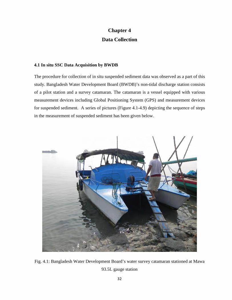
4.1 In situ SSC Data Acquisition by BWDB
The procedure for collection of in situ suspended sediment data was observed as a part of this
study. Bangladesh Water Development Board (BWDB)’s non-tidal discharge station consists
of a pilot station and a survey catamaran. The catamaran is a vessel equipped with various
measurement devices including Global Positioning System (GPS) and measurement devices
for suspended sediment. A series of pictures (Figure 4.1-4.9) depicting the sequence of steps
in the measurement of suspended sediment has been given below.
Fig. 4.1: Bangladesh Water Development Board’s water survey catamaran stationed at Mawa
93.5L gauge station
32
Page 51
Fig. 4.2: An automatic pulley system used to lift and submerge gauging equipment
Fig. 4.3: Sediment gauging equipment being prepared for sample collection
33
Page 52
Fig. 4.4: Sediment sampling equipment being lowered for water sample collection
Fig. 4.5: Sediment sampling equipment being lifted up after water sample collection
34
Page 53
Fig. 4.6: Water sample being transferred to another container from sediment sampling
equipment
Fig. 4.7: Sample being transferred from the container to the measurement tube using a funnel
35
Page 54
Fig. 4.8: Measurement tubes being separated after collection of sample
Fig. 4.9: Samples in measurement tubes being stored to be transferred to laboratory for
testing
The measurement protocol starts with spatially accurate placement and anchoring of survey
catamaran using GPS device. A measuring probe specifically designed for the purpose of
36
Page 55
collecting turbid water from rivers is lowered into the water through a gap at the middle of
the vessel with the aid of an automated pulley (Figure 4.4). The mouth of the probe is opened
and the device is sunk about 1-2 meters into the flowing river water. After about 2 minutes
the probe is lifted upwards and the water trapped inside of it is collected in a container
(Figure 4.5). A test tube is setup below a funnel in an upright platform and the sample water
is drained into it for exactly 1 minute (Figure 4.7). Thereafter the test tubes are sealed and
stored in crates (Figure 4.9) and transferred to BWDB’s lab where the concentration of
sediments and sediment sizes are recorded at a later time.
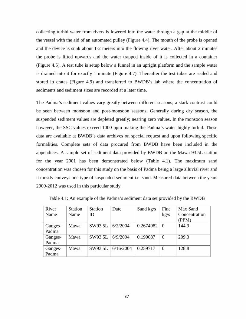
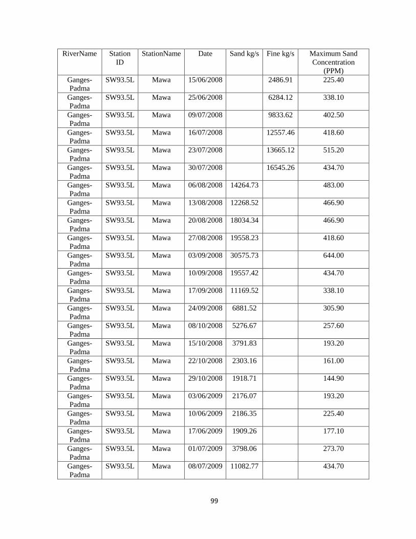
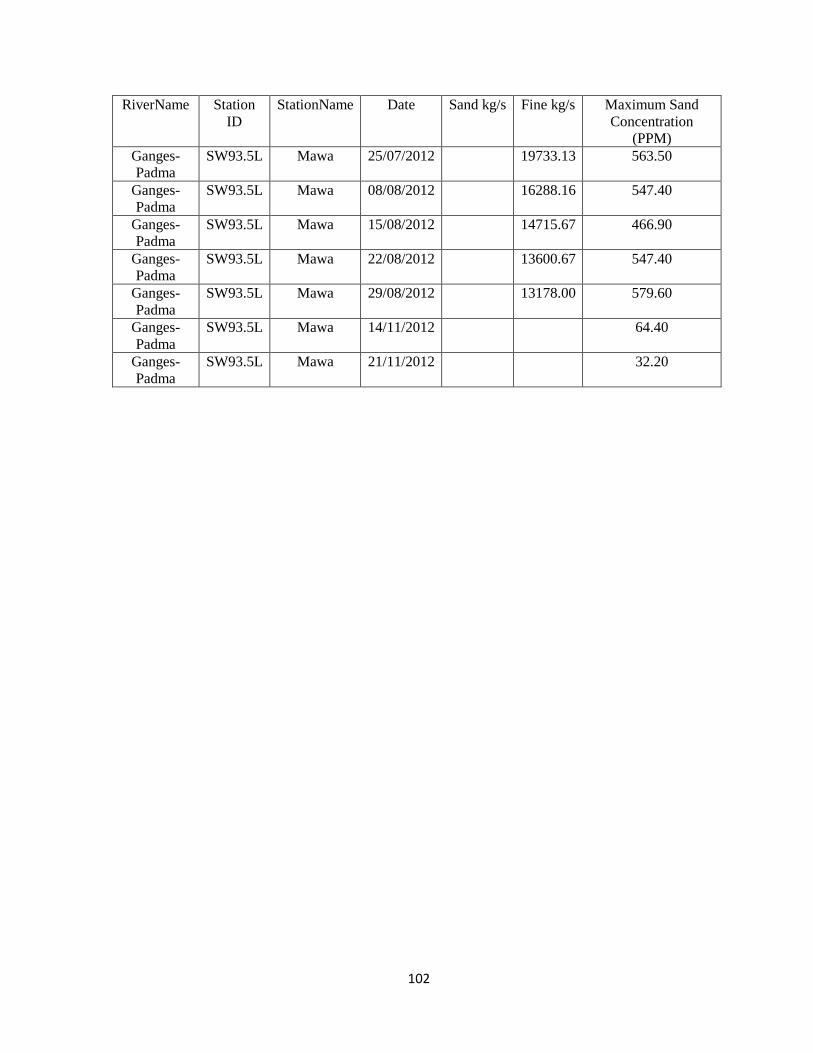
The Padma’s sediment values vary greatly between different seasons; a stark contrast could
be seen between monsoon and post-monsoon seasons. Generally during dry season, the
suspended sediment values are depleted greatly; nearing zero values. In the monsoon season
however, the SSC values exceed 1000 ppm making the Padma’s water highly turbid. These
data are available at BWDB’s data archives on special request and upon following specific
formalities. Complete sets of data procured from BWDB have been included in the
appendices. A sample set of sediment data provided by BWDB on the Mawa 93.5L station
for the year 2001 has been demonstrated below (Table 4.1). The maximum sand
concentration was chosen for this study on the basis of Padma being a large alluvial river and
it mostly conveys one type of suspended sediment i.e. sand. Measured data between the years
2000-2012 was used in this particular study.
Table 4.1: An example of the Padma’s sediment data set provided by the BWDB
River Name
Station Name
Station ID
Date Sand kg/s Fine kg/s
Max Sand Concentration (PPM)
Ganges-Padma
Mawa SW93.5L 6/2/2004 0.2674982 0 144.9
Ganges-Padma
Mawa SW93.5L 6/9/2004 0.190087 0 209.3
Ganges-Padma
Mawa SW93.5L 6/16/2004 0.259717 0 128.8
37
Page 56
4.2 Acquisition of Landsat Data
Landsat 7 Enhanced Thematic Mapper (ETM+) images were selected as the remotely sensed
data for this study. The Landsat’s temporal resolution is 16 days and its spatial resolution is
30 m, meaning that images for a specific path and row are available every 16 days. Landsat
being sun-synchronous, it generates day images only. These images are available for
download upon request from United States Geological Survey (USGS) specified websites
such as earthexplorer.usgs.gov and glovis.usgs.gov. For acquiring Landsat 7 data from its
historical data archives, earthexplorer.usgs.gov was chosen. USGS offers open access to
Level 1G product to users; L1G is a radiometrically and geometrically corrected Level 0R
image. The correction algorithms used the spacecraft model and sensor, using images
generated by in-flight computers during data acquisition events. Primary inputs are
the Payload Correction Data, which includes the attitude and ephemeris profiles,
the definitive ephemeris (if available) and the Mirror Scan Correction Data (MSCD).
Although terrain corrected L1Gt products were available upon special request, they were not
applicable for the current study which only deals with reflectance from surface water.
Landsat 7 captures visible bands in the spectrum of blue, green, red, near-infrared and mid-
infrared (bands 1-5 & 7). It is also equipped with thermal infrared channel (band 6) with a
spatial resolution of 60 m. Landsat 7 data were glitch-free up to 2003, then there was a
mechanical disturbance in the Scan Line Corrector (SLC); therefore images resulted in
partially missing data. However, the SLC error did not have any significant implication
regarding this study, and therefore correction was not necessary.
Upon creating an USGS EROS account at www.earthexplorer.usgs.gov an Email connection
was established between user and website. For access to desired data, the polygon of
corresponding image was selected by inputting Path and Row numbers of 137 and 44
respectively. This polygon covers the entire length of the Padma River and portions of the
Brahmaputra and Ganges inside Bangladesh. After selecting the desired date and type of
product an order was placed for processed L1G product. It is to be noted that the months of
June to September were considered to be in Monsoon season. October and November were
taken as post monsoon months. Thereafter download links were sent to user emails from
USGS EROS when the products were ready. The downloaded products were compressed in a
38
Page 57
zip file; upon expanding, images corresponding to the 8 bands of Landsat 7 were revealed
along with some other data files which included the metadata file consisting of relevant
information required in this study. Figure 4.10 shows an example of a true color composite
Landsat ETM+ image. List of all Landsat 7 ETM+ images used in this study have been
mentioned in appendix-F.
Fig. 4.10: Example of True Color Landsat 7 ETM+ Product (Polygon Path 137 & Row 44)
4.3 Hydro-morphological Data Collection
Water level, discharge, flow velocity and cross section data corresponding to sediment data
were also procured from the Bangladesh Water Development Board through appropriate
acquisition procedure. These data sets were used for morphological analyses later in this
study. Appendix-B contains these detailed data tables as provided by BWDB.
39
Page 58
Chapter 5 - Satellite Image Processing
5.1. Processing Landsat Data
Landsat ETM+ L1G products between the years 2000-2010 were processed for analysis in
this study. List of all Landsat data sets used in this study has been provided in the appendix
(Appendix-F) section. These images were selected based on two broad temporal categories,
i.e. monsoon and post-monsoon season images. The months of June to September were
considered to inside monsoon, whereas the months of October and November were deemed
to be in post-monsoon season. Landsat images were processed using ILWIS.
Integrated Land and Water Information System (ILWIS) is a remote sensing and GIS
software which integrates image, vector and thematic data in one unique and powerful
package on the desktop. ILWIS delivers a wide range of features including import/export,
digitizing, editing, analysis and display of data, as well as production of quality maps
(www.52north.org).
The procedure for extraction of Digital Number (DN) begins with the importing of Raster
images as Tagged Image File Format (.TIF). Input files are found in the folder containing
decompressed Landsat data corresponding to specific bands. Because bands 1-4 have been
proven by previous multiple researches to have the best relationship with suspended sediment
reflectance, as mentioned in previous chapters; only data corresponding to aforementioned
bands of specific wavelengths were imported. Upon importing, Raster Operation was
initiated and with the aid of MapList Calculation function, raster images corresponding to the
four bands were aggregated to be viewed as Color Composite images. To obtain True Color
Composite images, the bands Blue, Green and Red were mapped to their corresponding
layers. Thereafter, the pixel information window was accessed and the study area was
focused upon by zooming in on the coordinates Latitude 23° 28’ N and Longitude 90° 15’ E.
For each image, five cloud-free points across the length of the Padma River at Mawa 93.5L
station were chosen and their corresponding band pixel values were recorded. A screenshot
of the ILWIS interface has been provided later (Figure 5.1). The process was repeated for
each of the downloaded product until band-wise pixel values, corresponding to the study
40
Page 59
area, were acquired for all the downloaded L1G products. To ensure that no submerged sand
bar could interfere with the desired reflectance, band combination RGB=754 was used which
sharply separated land and water. Also band 4 is sensitive to shallow water depths
(Poonawala et al., 2006). Hazy portions of the images were avoided as much as possible.
Atmospheric correction was skipped because the individual images had very small angular
range and it is almost impossible to carry out effective atmospheric correction if in situ
atmospheric conditions are unknown (Wang and Lu, 2010). Thus, atmospheric correction
was considered to have minimal effect on upcoming correlation analyses.
Fig. 5.1: Screenshot of ILWIS while extraction of DN with pixel information
It is worthy stating that Landsat ETM+ DN values range between 0 to 255 because these
images are 8-bit data systems. Although these DNs are useful values, they are not physically
meaningful. Therefore DN values for the four bands and each individual image were
converted to physical values of radiance using the satellite’s in-built sensor calibration
parameters. Due to the enormous volume of data tables used for recording DN, the data
record tables have been attached in the appendix section (Appendix-C). The highlighted row
is the average of the DN from five individual data points for each of the four bands (B1-B4).
41
Page 60
5.2. Conversion of DN into Radiance
Transformation of raw Landsat ETM+ Digital Numbers into physical values of radiance
involves the following formula [1] (Fleiflea, 2013).
Lλ = ((Lmax – Lmin)/255)DN + Lmin [1]
Where, Lλ is the spectral radiance (m W cm-2 sr-1 μm-1), Lmax is the radiance measured at
detector saturation (m W cm-2 sr-1 μm-1) and Lmin is the lowest radiance (m W cm-2 sr-1 μm-1). The
radiance at detector saturation and lowest radiance values for bands of each image is
available inside their corresponding metadata files attached with L1G products.
5.3. Conversion of Radiance into Top of Atmosphere Reflectance
Top of Atmosphere or Exoatmospheric Reflectance corrects for the earth-sun distance and
solar angle errors. Reflectance is the proportion of the radiation striking a surface to the
radiation reflected off of it. Thus to increase the accuracy of results, it was preferable to
convert those radiance values into Exoatmospheric reflectance values. The following formula
[2] (Fleiflea, 2013) was used for conversion.
pλ = ( πd2Lλ / Eoλ cosθs) [2]
Where, pλ is the ToA or Exoatmospheric Reflectance as a function of the band width λ, d2 is
the factor which corrects the variation in solar irradiances due to varying earth-sun distance
at different times of the year. The value of d for each image was acquired from a table
provided by USGS which consists of d values corresponding to the day of year. Eoλ or Fi is
the mean solar Exoatmospheric Irradiance (Wμm-2); θs represents the Solar Zenith Angle in
radians which was obtained by subtracting the Solar Elevation Angle from 90 degrees.
To alleviate the volume of tasks regarding these two conversions of 32 Landsat ETM+
images, each with four bands, excel function sheets were created where input average DN
data was converted directly into reflectance values. The Earth-sun distance correction factor
(d) table provided by USGS/NASA has been attached in the appendix section (Appendix-D).
42
Page 61
The resultant Top of Atmosphere or Exoatmospheric Reflectance values for the bands (B1-
B4) corresponding to Day of Year between 2000 and 2010 have been listed in the table
below (Table 5.1). These band specific reflectance values were used in correlation and
regression analyses of this study. The application and significance of these data sets have
been discussed in next chapters.
Table 5.1: Resultant ToA reflectance (dimensionless) values
43
Page 62
YearDay of Year B1 B2 B3 B4
235 0.173 0.166 0.171 0.146283 0.159 0.148 0.137 0.114299 0.172 0.158 0.144 0.120331 0.184 0.164 0.144 0.164189 0.188 0.187 0.183 0.164221 0.175 0.171 0.167 0.146269 0.163 0.152 0.142 0.120256 0.163 0.159 0.152 0.122304 0.156 0.145 0.129 0.102227 0.175 0.165 0.167 0.131307 0.174 0.160 0.151 0.126323 0.171 0.157 0.143 0.162182 0.206 0.198 0.192 0.175230 0.200 0.196 0.191 0.176246 0.216 0.201 0.193 0.187294 0.105 0.103 0.098 0.112
2005 280 0.176 0.162 0.149 0.131139 0.157 0.147 0.132 0.101299 0.165 0.162 0.150 0.115270 0.162 0.160 0.159 0.130302 0.113 0.111 0.105 0.119334 0.173 0.161 0.138 0.143177 0.191 0.190 0.185 0.154209 0.173 0.174 0.174 0.153273 0.161 0.173 0.171 0.153289 0.169 0.162 0.155 0.128305 0.107 0.102 0.094 0.101163 0.206 0.196 0.183 0.148291 0.129 0.122 0.117 0.121182 0.187 0.181 0.175 0.156294 0.163 0.158 0.151 0.124
2010
2004
2006
2007
2008
2009
Mawa 93.5L ToA Reflectance
2000
2001
2002
2003
44
Page 63
Chapter 6 Development of SSC- Spectral Reflectance Relationships
6.1. Investigating SSC-ToA Reflectance for Individual Bands
To investigate which band or what combination of bands of Landsat ETM+ provide the
strongest correlations. For the purpose of analysis the ToA Reflectance values were
converted to ToA% values. Thereafter XY scatter plot were drawn for each of the four bands.
For each scatter plot, a best-fit polynomial curve was plotted and its Coefficient of
Determination (R2) was found out (Figure 6.1-6.4). The results have been demonstrated and
discussed below.
Fig. 6.1: Scatter plot of measured SSC versus ToA reflectance percentage of band 1
45
Page 64
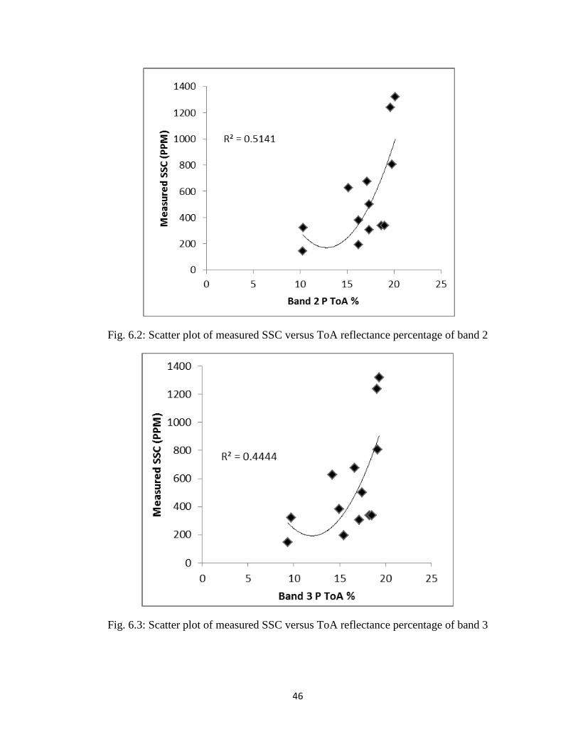
Fig. 6.2: Scatter plot of measured SSC versus ToA reflectance percentage of band 2
Fig. 6.3: Scatter plot of measured SSC versus ToA reflectance percentage of band 3
46
Page 65
Fig. 6.4: Scatter plot of measured SSC versus ToA reflectance percentage of band 4
The purpose of these correlation analyses is to investigate any statistically significant
relationship between two variables. In this case it was to investigate which band’s reflectance
values. R2 values indicate the strength of correlation; ranging between 0-1, the closer to 1 the
stronger is the agreement between two variables. R2 for bands 1, 2, 3 and 4 were 0.6359,
0.5141, 0.4444 and 0.6729 respectively. Although reflectance at band 1 shows significantly
strong relationship with measured SSC, band 4 (R2= 0.6729) demonstrated the strongest
statistical relationship among the four, which is consistent with previous studies (Sterckx et
al., 2007; Wass et al., 1997). Therefore band 4 (Near Infrared) was chosen as the indicator
for SSC. Near Infrared spectrum is sensitive to SSC and relative to shorter wavelength bands,
also less influenced by bottom reflectance in environments with shallow water (Tolk et al.,
2000). Owing to the non-linear nature of the data, curvilinear polynomial equation [3] was
chosen. The polynomial relationship obtained from the best-fit curve can be stated as,
SSC = 22.565 (B4)2 - 549.27(B4) + 3616.7 [3]
Where ‘SSC’ is the Suspended Sediment Concentration (ppm) and ‘B4’ is the Band 4 ToA
reflectance percentage. Polynomial relationship, which provided the best coefficient of
47
Page 66
determination values, was chosen over linear (Figure 6.5), exponential (Figure 6.6) and log
formulations (Figure 6.7), after applying them similarly to examine the relationship between
SSC and reflectance percentage values. In order to validate the regression relation between
SSC and band 4 reflectance percentage values, scatter plot of predicted values of SSC from
equation [3] versus measured values of SSC was drawn and the Root Mean Square Error
(RMSE) was extracted (Figure 6.8). Thereafter the residuals were also plotted against
measured SSC (Figure 6.9). Relative error percentage was also demonstrated in an individual
plot (Figure 6.10). A set of 13 Landsat ETM+ images were used to extract the estimated SSC
and corresponding measured values were used for this purpose have been provided in table
6.1.
Fig. 6.5: Scatter plot of measured SSC versus ToA reflectance percentage of bands 1-4 with
linear trend lines
48
Page 67
Fig. 6.6: Scatter plot of measured SSC versus ToA reflectance percentage of bands 1-4 with
exponential trend lines
49
Page 68
Fig. 6.7: Scatter plot of measured SSC versus ToA reflectance percentage of bands 1-4 with
logarithmic trend lines
50
Page 69
Table 6.1: Data sets used for validation of polynomial model [3]
Fig. 6.8: Scatter plot of estimated SSC values by the polynomial model based on band 4
(Near Infrared) ToA reflectance and measured SSC data with 1:1 fit line. (R2=0.89, n=13)
Date Measured SSC (ppm) Estimated SSC (ppm) Residuals (ppm) Squared Residuals RMSE Relative Error %1-Jul-10 460 543 -83 6889 -18.0
21-Oct-10 250 275 -25 625 -10.012-Jun-09 435 434 1 1 0.018-Oct-09 194 273 -79 6241 -40.74-Aug-05 1047 1214 -167 27889 -15.917-Jun-05 194 278 -84 7056 -25.32-Jun-11 225 282 -57 3249 -39.6
22-Sep-11 837 717 120 14400 14.38-Oct-11 644 525 119 14161 18.5
24-Oct-11 274 287 -13 169 -4.720-Jun-12 354 276 78 6084 22.022-Jul-12 564 595 -31 961 -5.57-Aug-12 548 665 -117 13689 -21.0
88.3
R² = 0.8928
0
200
400
600
800
1000
1200
1400
0 200 400 600 800 1000 1200
Estim
ated
SSC
(ppm
)
Measured SSC (ppm)
51
Page 70
Fig. 6.9: Residue of SSC versus measured SSC
Fig. 6.10: Scatter plot of relative error percentage of estimated SSC from measured SSC (Average relative error is ±18.11%)
Scatter plot of predicted SSC values from the polynomial equation [3] against in situ values
of SSC with 1:1 fit line generated strong positive coefficient of determination of 0.89 and
Root Mean Square Error (RMSE) of 88.3 ppm. The residual values of SSC were calculated
by subtracting estimated values of SSC from the measured data. RMSE was extracted by
-400
-300
-200
-100
0
100
200
300
400
0 200 400 600 800 1000 1200
Resi
dual
SSC
(ppm
)
Measured SSC (ppm)
-50
-40
-30
-20
-10
0
10
20
30
40
50
0 200 400 600 800 1000 1200
Rela
tive
Erro
r %
Measured SSC (ppm)
52
Page 71
calculating the square root of average squared residual. Therefore, predicted values and
measured values of SSC are in strong statistical agreement (Taylor, 1990), and that
correlation does imply causation for the polynomial relationship. It is apparent that this
model’s prediction accuracy is better for higher values of SSC i.e. above 200 ppm to
approximately 800 ppm. From the measured values of SSC, it is observed, the Padma River’s
SSC values usually range above 200 ppm for most of the time during monsoon and even
during post-monsoon season; thus affirming this model’s applicability. The average relative
error is ±18.11%.
6.2. Investigating Robust SSC- Spectral Reflectance Relationship
Some laboratory studies dealing with reflectance and SSC relationships suggested robust
SSC-Reflectance relationships throughout the visible portion of the spectrum may augment
the applicability of such models (Novo et al., 1989; Schiebe et al., 1992). Robust
relationships are especially important in cases where sediment color varies greatly. Some
studies have previously reflectance in the red band in combination with other reflectance of
other visible bands to augment the models’ robustness in the prospect of variation in
suspended sediment color (Aranuvachapun and Walling, 1988; Dekker et al., 2001; Han et
al., 2006; Lathrop et al., 1991; Wu et al., 2007). Padma being a large alluvial river, its
overall sediment color remains relatively unvaried; the alluvial at the foothills of eastern
Himalayas are formed by deposition from the north Bengal tributaries of the Ganges and
Brahmaputra, these rivers have also dissected the Barind tract, and therefore coarse-grained
sediments such as cobbles and sand dominate the Padma (Mukherjee et al., 2009). The four
band reflectance percentage values were used as independent variables and measured SSC
values were considered as dependent variables. The summary of multiple regression analysis
has been listed below (Table 6.2-6.4). Graphical representation of this analysis is also
provided (Figure 6.11).
53
Page 72
Table 6.2: Output table of regression analyses
Table 6.3: Summary of outputs of regression analyses
Regression Statistics Multiple R 0.867 R Square 0.753 Adjusted R Square 0.629 Standard Error 227.632 Observations 13
Table 6.4: Residual output of regression analyses
Coefficients Standard Error t Stat P-value Lower 95% Upper 95%Intercept -931.07 579.39 -1.61 0.15 -2267.15 405.01B1 PToa% 280.62 182.26 1.54 0.16 -139.68 700.91B2 PToA% -473.49 568.76 -0.83 0.43 -1785.05 838.08B3 PToA% 114.44 404.98 0.28 0.78 -819.44 1048.31B4 PToA% 186.85 70.10 2.67 0.03 25.20 348.50
Observation Predicted SSC (PPM) Residuals1 655.01 -316.912 499.04 177.163 344.06 283.844 960.71 -155.715 886.83 352.876 1302.00 18.207 357.19 -35.198 503.95 -123.459 440.14 -102.0410 543.42 -43.4211 208.64 97.2612 309.35 -116.1513 181.38 -36.48
54
Page 73
Fig. 6.11: Bands 1-4 ToA reflectance percentage plot
Multiple regression analysis allowed the investigation of how multiple independent variables
were related to dependent variables. From the results of regression analyses, a robust model
[4] can be derived.
SSC= -931.07 + 280.62B1 - 473.49B2 + 114.44B3 + 186.85B4 [4]
0
200
400
600
800
1000
1200
1400
0 20 40
SSC
(PPM
)
B1 Ptoa%
SSC (PPM)
Predicted SSC(PPM)
0
200
400
600
800
1000
1200
1400
0 10 20 30
SSC
(PPM
)
B2 PToA%
0
200
400
600
800
1000
1200
1400
0 10 20 30
SSC
(PPM
)
B3 PToA%
0
200
400
600
800
1000
1200
1400
0 5 10 15 20
SSC
(PPM
)
B4 PToA%
55
Page 74
Where, B1, B2, B3 and B4 are ToA reflectance percentage of respective bands. SSC can be
estimated by inputting top of atmosphere reflectance percentage (PToA%) of corresponding
four bands. However, the predictive values (P-value) of the Exoatmospheric reflectance
percentage of bands 1, 2 and 3 were above 0.15; which are very insignificant and therefore
can be omitted from the linear model (Lunt, 2015). Only band 4 reflectance percentage
possessed P-value low enough to be significant in predicting SSC values. Sediment color is
an integral factor when considering robust models for sediment mapping; due to lack of
ground-based spectrometer and hyperspectral images, there are no reliable measured
sediment color data available. Principle sources of uncertainty in these robust relationships,
within a study area, are differences in mineralogy, grain sizes as well as color (Choubey,
1998; Novo et al., 1991). Considering the aforementioned facts, the robust model [4] was
not considered for spatio-temporal mapping of SSC in the Padma River.
56
Page 75
Chapter 7
Spatio-temporal Variation of SSC
7.1 Retrieval of Spatial Distribution of SSC
To demonstrate the spatial and temporal variations of SSC in the Padma River, the
previously developed polynomial relationship (3) was applied. A sum of 18 Landsat ETM+
images from both monsoon and post-monsoon seasons, between years 2000 to 2010, were
used for this purpose. Landsat 7 ETM+ data were initially acquired from USGS specified
website, i.e. www.earthexplorer.usgs.gov as compressed files and then extracted to reveal the
images corresponding different bands. Quantum GIS (QGIS) was used for processing the
images. QGIS is an Open Source Geographic Information System (GIS) licensed under the
General Public License. QGIS is an official project of the Open Source Geospatial
Foundation (OSGeo). It runs on Linux, Unix, Mac OSX, Windows and Android and supports
numerous vector, raster, and database formats and functionalities (www.qgis.org).
Raster images corresponding to band 4 (wavelength: 0.77-0.90µm) were imported into the
QGIS software and cropped to magnify the area under focus. For each image, a vector layer
was created and the water body of the Padma River, extending up to approximately 20 km
upstream and 20 km downstream of BWDB Gauge Station Mawa 93.5L, was extracted. This
interactive process, in which a segment map is shaped while a raster map is displayed in the
background, is conventionally known as On-Screen Digitization. Using the extracted raster
image, SSC spatial distribution maps were created. For this purpose, raster calculation was
applied - where the raw digital number (DN) was first converted to spectral radiance using
the appropriate conversion formula, and then to Top of Atmosphere (ToA) reflectance
percentage. The resultant reflectance percentage values were input into the polynomial
relationship (3) to reveal the SSC values for each pixel. For facilitating visualization,
continuous Pseudocolor images were created. Sand bars and cloud patches were excluded
from the maps since their presence would disrupt the actual representation of SSC
distribution.
57
Page 76
Landsat 7 ETM+ images were error free up to May 31, 2003. Since then, the Scan Line
Corrector (SLC) which compensates for the forward motion of Landsat 7 ETM+ has failed,
resulting in duplicated image area and width that increases towards the edge of the images.
Therefore, all images acquired after May 2003 is accompanied by SLC error; this mode is
also referred to as SLC-off mode. However, the SLC-off mode did not hamper the effective
depiction of SSC distribution of the Padma River in this study. Coordinate Reference System
(CRS) was set to WGS 84/ UTM Zone 46N for both layer and project files. There was
particular difficulty in obtaining cloud-free Landsat images during monsoon season; and as a
consequence, there were no suitable images for demonstrating SSC spatial distribution for
the monsoon of 2003, 2009 and 2010. However, suitable post-monsoon images were
available for all of the years between 2000 and 2010. The resultant maps have been shown in
figures 7.1-7.18. Since coefficients of the polynomial relationship (3) is based on a single
station and confined to monsoon and post monsoon seasons, some errors may be expected
while computing Spatio-temporal distribution of SSC in the Padma River.
58
Page 77
7.2 Spatial Distribution Maps of SSC in the Padma River
Spatial distribution maps of SSC in the Padma River, from the year 2000 to 2010 (Figures
7.1-7.18), and their respective discussions are given below.
Fig. 7.1: Spatial distribution map of SSC in the Padma River for Monsoon of 2000
The Landsat scene identification number used for this spatial distribution map (Figure 7.1)
was LE71370442000283SGS00 (Image courtesy of the U.S. Geological Survey). The SSC
values ranged between 250-400 ppm. There was no significant cloud patch over the water
body of the river. The sand bars excluded from the map have been marked appropriately. A
notable rise of suspended sediment concentrations can be observed immediately downstream
of sand bars; an observation which may be attributed to erosive effect of the river. Another
interesting observation in this map is the sand bar, which apparently is situated at the margin
where water flows from the Ganges and Brahmaputra conflate, was not subjected to the
59
Page 78
erosive effect of the river, contrary to the observed behavior of sand bars downstream. The
detailed processes responsible for the formation of a braided river are still poorly understood.
Many published works deal specifically with the process of braiding, but little agreement can
be found, and the hydraulic parameters of a braided stream are extremely complex (Coleman,
1969).
Fig. 7.2: Spatial distribution map of SSC in the Padma River for Post Monsoon of 2000
The Landsat scene identification number used for this spatial distribution map (Figure 7.2)
was LE71370442000331SGS00 (Image courtesy of the U.S. Geological Survey). Compared
to the monsoon image shown previously (Figure 7.1), slight decline in SSC levels can be
observed; in this post-monsoon map, the SSC levels varied between 250-350 ppm. Also, in
contrast with the previous map, the sand bars are not facing erosion apparently. The average
measured discharge of Padma River at Mawa for monsoon season of 2000 was 63519 m3/s,
and the average measured discharge for the corresponding post-monsoon season was 38028
60
Page 79
m3/s. The average water flow velocity declined from 3.06 m/s in monsoon to 2.30 m/s in
post-monsoon season. These declines in discharge and flow velocity could be driving factors
behind the decline of sand bar erosion. There was also a decline of measured average water
level at Mawa 93.5L of more than 1 m between monsoon and post-monsoon seasons, also
possibly influencing erosion. The decline of SSC levels may be attributed to declines in
discharge, water level and flow velocity (Bogárdi and Szilvássy, 1974).
Fig. 7.3: Spatial distribution map of SSC in the Padma River for Monsoon of 2001
The Landsat scene identification number used for this spatial distribution map (Figure 7.3)
was LE71370442001269SGS00 (Image courtesy of the U.S. Geological Survey). SSC values
in this map varied between 250-400 ppm; quite similar to the SSC distribution of 2000
monsoon. Although some sporadic erosion of sand bars can be observed, they are not
significantly visible like the monsoon map of previous year (Figure 7.1). This reduced
erosion rate can again be attributed to reduced average monsoon discharge and flow velocity
61
Page 80
– the average monsoon discharge and flow velocity for monsoon 2001 were 46784 m3/s and
2.41 m/s respectively. Suspended Sediment - Discharge relations are influenced by multiple
factors - precipitation intensity and areal distribution, runoff amount and rate, floodwater
travel rates and travel distances, spatial and temporal storage-mobilization-depletion
processes of available sediment, and sediment travel rates and distances (Williams, 1989).
The Ganges and Brahmaputra River flows combine to form the Padma River. Flow from the
Ganges, adjacent to the left bank in the upstream (u/s) direction, seemed to be transporting
greater concentration of suspended sediments compared to the flow from the Brahmaputra.
The two flows can be delineated considering the stark difference between SSC levels of the
Ganges and the Brahmaputra flows.
Fig. 7.4: Spatial Distribution Map of SSC in Padma River for Post Monsoon of 2001
The Landsat scene identification number used for this spatial distribution map (Figure 7.4)
was LE71370442001333SGS00 (Image courtesy of the U.S. Geological Survey). SSC values
62
Page 81
in this map varied between 250-325 ppm – slightly lower than the maximum SSC during the
post-monsoon season of previous year (Figure 7.2). The average measured discharge and
flow velocity for post-monsoon of 2001 were 42045 m3/s and 2.13 m/s respectively; slightly
lower than the monsoon season (Figure 7.3). Although some bank erosion can be seen,
significant sand bar erosion was not apparent; possibly due to the nearly unchanged average
discharge and flow velocity (Bogárdi and Szilvássy, 1974). Also measured average water
level did not change significantly between monsoon and post monsoon seasons of 2001.
Fig. 7.5: Spatial distribution map of SSC in the Padma River for Monsoon of 2002
The Landsat scene identification number used for this spatial distribution map (Figure 7.5)
was LE71370442002256SGS00 (Image courtesy of the U.S. Geological Survey). It must be
noted that in this map, excluding the designated sand bars, the missing patches towards are
bank are cloud covers. A significant rise of SSC level can be seen for 2002 monsoon. This
rise may be due to increased discharge, water level or flow velocity considering the
63
Page 82
prevalence of a monsoon flood in 2002. However, there is no definitive data available on the
aforementioned parameters for this map. In this map again, the flow from the Ganges and the
Brahmaputra can be delineated based on their sharp difference in SSC levels. The Ganges
seemed to be contributing higher levels suspended sediment concentration into the Padma
compared to the Brahmaputra.
Fig. 7.6: Spatial distribution map of SSC in the Padma River for Post Monsoon of 2002
The Landsat scene identification number used for this spatial distribution map (Figure 7.6)
was LE71370442002304SGS00 (Image courtesy of the U.S. Geological Survey). Although
the SSC levels in this map are higher than the post monsoon seasons of previous years, a
significant amount of sand bar erosion can be observed. Since there are no reliable in situ
data available corresponding to this map, the erosive behavior cannot be exactly attributed to
certain hydro-morphological aspects.
64
Page 83
Fig. 7.7: Spatial distribution map of SSC in the Padma River for Post Monsoon of 2003
The Landsat scene identification number used for this spatial distribution map (Figure 7.7)
was LE71370442003323ASN01 (Image courtesy of the U.S. Geological Survey). There was
no suitable cloud-free monsoon image for appropriate depiction of SSC distribution,
therefore only post-monsoon image was chosen. As mentioned earlier, SLC-off mode caused
the line errors in the maps starting from 2003. Compared to the post monsoon SSC values of
previous year, there was some decline noticeable for 2003. However, levels of SSC for post
monsoon of 2003 seem to be higher compared to post monsoon of 2000 (Figure 7.2) and
2001 (Figure 7.4); again this may be because measured average water level, discharge and
flow velocity were higher. Contrary to previous observations, flow contributed by the
Brahmaputra had higher SSC compared to the flow contributed by the Ganges. There is
appearance of aggradation of channel bars downstream of the image. Aggradation and
degradation are generally influenced by river discharge, sediment load, morphological
characteristics of river channel and human interventions; if the river water is unable to
65
Page 84
transfer the bed load or the channel material then the same is deposited within the channel
and channel height increases, aggradation occurs (Mugade and Sapkale, 2015).
Fig. 7.8: Spatial distribution map of SSC in the Padma River for Monsoon of 2004
The Landsat scene identification number used for this spatial distribution map (Figure 7.8)
was LE71370442004230PFS01 (Image courtesy of the U.S. Geological Survey). Although
there were multiple patches of cloud over the body of the river, this image bared evidence of
a sharp rise in SSC levels in the 2004 flood. This image in particular was acquired during
flood condition. Minimum SSC in this map was about 400 ppm, but the highest SSC value
was over 2000 ppm. The most intensive transport processes in rivers occur during the
passage of a flood wave (Rowiński and Czernuszenko, 1998). Sediment transport is usually
different in unsteady flow during flood events (Tabarestani and Zarrati, 2015). There was no
in situ data acquired by BWDB during the flood season. The average monsoon water levels
66
Page 85
of 5.20 m, discharge of 63414 m3/s and flow velocity of 2.64 m/s were not truly
representative of the flood conditions.
Fig. 7.9: Spatial distribution map of SSC in the Padma River for Post Monsoon of 2004
The Landsat scene identification number used for this spatial distribution map (Figure 7.9)
was LE71370442004294PFS01 (Image courtesy of the U.S. Geological Survey). Compared
to the SSC spatial distribution map during monsoon flood, the post monsoon map showed
dramatic decrease in overall SSC. Sand bar erosion was not a prominent feature of this map
and measured morphological parameters such as average water level, discharge and flow
velocity, although attenuated a little, did not change notably compared to the post monsoon
map of previous year (Figure 7.7).
67
Page 86
Fig. 7.10: Spatial distribution map of SSC in the Padma River for Monsoon of 2005
The Landsat scene identification number used for this spatial distribution map (Figure 7.10)
was LE71370442005152PFS00 (Image courtesy of the U.S. Geological Survey). The
maximum SSC level for this map was about 600 ppm. Owing to the presence of patches of
clouds, this map does not depict the true variation of SSC on that day. Shadows cast by cloud
patches also resulted in irregular variations of SSC in the map, which can be considered as
errors or limitations while representing SSC variation through spatial maps.
68
Page 87
Fig. 7.11: Spatial distribution map of SSC in the Padma River for Post Monsoon of 2005
The Landsat scene identification number used for this spatial distribution map (Figure 7.11)
was LE71370442005294PFS00 (Image courtesy of the U.S. Geological Survey). The most
prominent feature of this map is the unusually different SSC levels between flow contributed
by the Ganges and the Brahmaputra. The Ganges flow, which merges from the eastern
upstream direction, is clearly higher in suspended sediments, and it is not till further
downstream, the sediments diffuse. In a large alluvial river, like the Padma, the constraints
imposed by the capacity of flow to transport sediments reflect upon suspended-sediment
transport, sediment flux and the longitudinal profile of the channel (Dade and Friend, 1998).
69
Page 88
Fig. 7.12: Spatial distribution map of SSC in the Padma River for Post Monsoon of 2006
The Landsat scene identification number used for this spatial distribution map (Figure 7.12)
was LE71370442006283PFS00 (Image courtesy of the U.S. Geological Survey). Compared
to the post monsoon of 2005 (Figure 7.11), the maximum SSC value for this image decreased
notably. Contrary to 2005, in this image, the Brahmaputra appears to be contributing higher
suspended sediment concentration compared to flow from the Ganges. An interesting
observation is a vortex-like secondary flow pattern at the upstream portion of the image.
Such pattern of flow is a common phenomenon in alluvial rivers and associated with the
complex process of scouring (Lagasse et al., 2012).
70
Page 89
Fig. 7.13: Spatial distribution map of SSC in the Padma River for Monsoon of 2007
The Landsat scene identification number used for this spatial distribution map (Figure 7.13)
was LE71370442007270PFS00 (Image courtesy of the U.S. Geological Survey). In this map,
SSC values ranged between 275 to 375 ppm. There are no in situ data of corresponding water
level, discharge or flow velocity data available for this image. However, compared to
previous monsoons, SSC values were considerably lower for this particular image.
71
Page 90
Fig. 7.14: Spatial distribution map of SSC in the Padma River for Post Monsoon of 2007
The Landsat scene identification number used for this spatial distribution map (Figure 7.14)
was LE71370442007334PFS00 (Image courtesy of the U.S. Geological Survey). Conflicting
previous observations, this post monsoon image has higher SSC range compared to the
monsoon season. Even though there are no corresponding in situ discharge, water level and
flow velocity data available for this image, the rise in post monsoon sediment transport may
be possibly due to increased flow in delayed monsoon (Mirza, 2002).
72
Page 91
Fig. 7.15: Spatial distribution map of SSC in the Padma River for Monsoon of 2008
The Landsat scene identification number used for this spatial distribution map (Figure 7.15)
was LE71370442008209SGS01 (Image courtesy of the U.S. Geological Survey). SSC range
varied between 300 to 750 ppm for this image. This increase is expected due to increase in
average discharge, flow velocity and water level compared to the previous monsoon (Bogárdi
and Szilvássy, 1974).
73
Page 92
Fig. 7.16: Spatial distribution map of SSC in the Padma River for Post Monsoon of 2008
The Landsat scene identification number used for this spatial distribution map (Figure 7.16)
was LE71370442008305SGS01 (Image courtesy of the U.S. Geological Survey). Owing to
decreases in water level, discharge and flow velocity, the maximum SSC also declined
compared to corresponding monsoon season (Bogárdi and Szilvássy, 1974). Some
differences in upstream and downstream SSC levels can be seen. These observations may
possibly be due to variations in sediment settling rate and boundary layer shear stress (Van
Rijn, 1993).
74
Page 93
Fig. 7.17: Spatial distribution map of SSC in the Padma River for Post Monsoon of 2009
The Landsat scene identification number used for this spatial distribution map (Figure 7.17)
was LE71370442009339SGS00 (Image courtesy of the U.S. Geological Survey). The post
monsoon of 2009 saw an increase in average measured water level, discharge and flow
velocity compared to the monsoon season. Therefore, the suspended sediment concentration
rate was unexpectedly high as well, in agreement with known theories (Bogárdi and
Szilvássy, 1974). The anomalous monsoon delay has become a noticeable observation in the
advent of unnatural weather patterns in the face of climate change, and it is found to be
responsible for unexpected rise of river flow and sediment transport in rivers (Bookhagen et
al., 2005).
75
Page 94
Fig. 7.18: Spatial distribution map of SSC in the Padma River for Post Monsoon of 2010
The Landsat scene identification number used for this spatial distribution map (Figure 7.18)
was LE71370442010294SGS00 (Image courtesy of the U.S. Geological Survey). Compared
to the monsoon of 2010 (Figure 7.17), the post monsoon levels of SSC declined with
attenuating average discharge, water level and flow velocity. Suspended sediment transport
patterns show erosion or degradation of sand bars in this image. These processes are
complex (Middleton and Southard, 1984) and require more extensive analyses.
76
Page 95
7.3 Temporal Variation of SSC at Mawa
To observe how average monsoon and post monsoon SSC values varied at the Mawa, SW
93.5L station at the Padma River, the temporal variation of SSC between the years 2000 and
2010 was plotted (Figure 7.19).
Fig. 7.19: Temporal variation of SSC
7.3 Relationship between SSC and Cross-section of River
To observe any existing relationship between spatial variations of SSC and measured cross
section of the Padma River at Mawa, SSC values corresponding to cross sectional distance
were recorded. The results have been shown in figures 7.20-7.23.
77
Page 96
Fig. 7.20: Variation of cross section and corresponding SSC for Post Monsoon of 2001
Fig. 7.21: Variation of cross section and corresponding SSC for Monsoon of 2002
78
Page 97
Fig. 7.22: Variation of cross section and corresponding SSC for Post Monsoon of 2005
Fig. 7.23: Variation of cross section and corresponding SSC for Post Monsoon of 2008
79
Page 98
The cross-sectional data acquired for 2001 Post Monsoon (Figure 7.20) is from BWDB’s
River Maintenance Project (RMP)-6. For 2002 Monsoon (Figure 7.21), the cross-sectional
data was recorded during RMP-4, and for Post Monsoon of 2005 (Figure 7.22) and 2008
(Figure 7.23), cross sectional data was recorded during RMP-7. It can be observed from all
the four plots that SSC rises, albeit through variable range, whenever the Reduced Level
(RL) value rises. SSC tends to increase with depth, and when bed level rises, the
corresponding SSC also tends to increase (Okada, 2016). Although near-infrared
wavelengths of band 4 of Landsat 7 ETM+ is less susceptible to be influenced by shallow
water environments (Tolk et al., 2000), there may still be some degree of influence during
changes in water depth. This phenomenon maybe a limitation when remotely sensed SSC is
used to assess changes in water depth (Gao, 2009).
7.4 Measured Average Discharge, Water Level and Flow Velocity at Mawa 93.5L
The measured average monsoon and post monsoon data of discharge, water level (WL) and
flow velocity at Mawa 93.5L gauging station, used for interpretation of spatial distribution
maps of SSC have been represented in figures 7.24-7.26. Historical data sets provided by
BWDB have been included in the appendix section (Appendix-B).
Fig. 7.24: Measured average yearly discharge at Mawa 93.5L
80
Page 99
Fig. 7.25: Measured average yearly water level at Mawa 93.5L
Fig. 7.26: Measured average yearly flow velocity at Mawa 93.5L
81
Page 100
7.5 Relationship between Measured SSC and Flow Velocity
To investigate whether measured values of flow velocity have any statistical relationship
with in situ values of SSC, a correlation analysis (Figure 7.29) was carried out. The result has
been depicted below.
Fig. 7.27: Scatter plot of maximum flow velocity and measured SSC
A logarithmic trendline generated moderate coefficient of determination of 0.3689. The
following logarithmic model [6] was derived.
Flow Velocity = 0.6814ln(SSC) – 1.5434 [6]
Using the logarithmic model [6], measured values of SSC were used to estimate
corresponding flow velocity. The estimated values were then compared with actual values to
assess this model’s accuracy. The average relative error between estimated and observed
values was found to be ±14.93%. Results have been represented in table 7.1.
R² = 0.3689
0.0
0.5
1.0
1.5
2.0
2.5
3.0
3.5
4.0
0 200 400 600 800 1000 1200 1400
Max
imum
Vel
ocity
(m
/s)
Measured SSC (ppm)
82
Page 101
Table 7.1: Relative error assessment of estimated flow velocity using [6]
As the average relative error was less than 15%, the model [6] was used to generate spatial
distribution maps from corresponding spatial variation maps of SSC. The two maps chosen
were 2000 Monsoon and 2002 Post Monsoon. After appropriate conversions using raster
calculation in GIS software, the two maps (Figure 7.28 and 7.29) were rendered. This
practice may be considered an example on the application of Landsat images to observe
spatial variation of flow velocity in large alluvial rivers.
Measured SSC (ppm) Measured Velocity (m/s) Estimated Velocity (m/s) Residuals Relative Error %225.4 1.8 2.1 -0.4 -20.8257.6 1.9 2.2 -0.4 -18.5450.8 3.0 2.6 0.4 12.8563.5 2.9 2.8 0.1 4.0579.6 3.0 2.8 0.2 7.5627.9 3.2 2.8 0.4 11.4595.7 3.5 2.8 0.6 18.7644.0 3.5 2.9 0.6 17.7885.5 2.7 3.1 -0.4 -15.9805.0 2.6 3.0 -0.4 -15.2837.2 3.0 3.0 0.0 -0.9788.9 2.7 3.0 -0.3 -9.4724.5 2.7 2.9 -0.3 -10.5644.0 2.2 2.9 -0.7 -32.7483.0 1.8 2.7 -0.9 -51.8273.7 1.6 2.3 -0.7 -41.7241.5 1.6 2.2 -0.5 -33.2354.2 2.1 2.5 -0.4 -17.4483.0 2.7 2.7 0.1 1.9563.5 3.2 2.8 0.4 13.1547.4 2.8 2.8 0.0 1.5466.9 2.7 2.6 0.0 1.1547.4 2.6 2.8 -0.1 -4.2579.6 2.5 2.8 -0.3 -11.8
83
Page 102
Fig 7.28: Spatial variation of flow velocity for monsoon of year 2000
Fig 7.29: Spatial variation of flow velocity for post monsoon of year 2002
84
Page 103
Chapter 8 Conclusions and Recommendations
8.1 Conclusions
Landsat ETM+ images were used in combination with available in situ values of SSC to
develop a model for retrieving temporal values of SSC at the Padma River in Bangladesh.
The analysis saw extraction of DN from Landsat data and their conversion to spectral
radiance values. The radiance values were then transformed into ToA Reflectance or
Exoatmospheric Reflectance values using appropriate conversion formulae. Thereafter
regression methods were applied to investigate statistical relationship between ToA
reflectance percentage and corresponding in situ values of SSC; Band 4 (0.76-0.90 μm) ToA
reflectance % values proved to be the most sensitive and suitable indicator of SSC for the
Padma River.
For validation of the polynomial model involving SSC and Band 4 Reflectance Percentage
values, scatter plot of predicted values of SSC from the model versus measured values of
SSC was drawn and the Root Mean Square Error (RMSE) was extracted. Scatter plot of
predicted SSC values from the polynomial equation (3) against in situ values of SSC with 1:1
fit line generated strong positive coefficient of determination (R2) of 0.89 and Root Mean
Square Error (RMSE) of 88.3 ppm. Because predicted values and measured values of SSC
were in strong statistical agreement, polynomial model based on the band 4 data was selected
to estimate monsoon and post-monsoon spatial variations of SSC for the years 2000 to 2010.
Assessment of applicability of a robust relationship, combining bands 1-4, through multiple
regression analysis was also carried out. However, the predictive values (P-value) of the ToA
Reflectance percentage of bands 1, 2 and 3 were very insignificant; only band 4 reflectance
percentage possessed P-value low enough to be significant in predicting SSC values. The
robust model was therefore not considered further on.
Spatial distribution maps of SSC, between years 2000 and 2010 were observed. Among the
notable observations, overall SSC levels appeared to be generally higher in monsoon and
flood seasons compared to post-monsoon season. However, there were exceptions in this
85
Page 104
observation too. Rise in discharge, water level and flow velocity increased the overall SSC.
During cross-section analysis, it was generally observed that rise in bed level also caused
small jumps in SSC levels.
Using statistical correlation analysis of measured values of SSC and corresponding in situ
values of maximum flow velocity, a logarithmic relationship model were derived. Using this
model and spatial distribution maps of SSC, spatial variation maps of maximum flow
velocity was created. This exercise was conducted as an example on application of satellite
remote sensing.
The task of obtaining and reliable and constant spatial and temporal SSC data of rivers in
Bangladesh is severely constrained. These limitations include size and extent of rivers,
financial and economic constraints; lack of experienced personnel. Although in situ
measurement techniques of suspended sediment are continually changing, it is generally
accepted that they do not completely satisfy requirements. This study has shown a way in
which these problems can be alleviated with the help of satellite remote sensing. The
polynomial relationship developed in this study is the first of its kind for the large alluvial
Padma River, and it presents room for further development of such relations for the other
rivers of Bangladesh.
8.2 Recommendations
It may be recommended to further augment the applicability of this study by integrating
similar models for the Ganges and Brahmaputra Rivers. It is also recommended that more
data measurement points be introduced along the Padma River to know the spatial variability
of coefficients of the polynomial relationship [3]. In situ atmospheric data at the data point is
expected to further bolster the validity of such models. Spatial distribution maps of SSC can
be useful tools of improving the understanding of sediment transport patterns in the Padma
River. It is recommended that further in situ studies be carried out in conjunction with spatio-
temporal mapping of SSC to better understand hydro-morphological process in the Padma
River and the greater GBM delta.
86
Page 105
References
Alam, M., Alam, M.M., Curray, J.R., Chowdhury, M.L.R. and Gani, M.R., 2003. An
overview of the sedimentary geology of the Bengal Basin in relation to the regional
tectonic framework and basin-fill history. Sedimentary Geology, 155(3): 179-208.
Allison, M.A., 1998. Historical Changes in the Ganges-Brahmaputra Delta Front. Journal of
Coastal Research, 14(4): 1269-1275.
Aranuvachapun, S. and LeBlond, P.H., 1981. Turbidity of coastal water determined from
Landsat. Remote Sensing of Environment, 11: 113-132.
Aranuvachapun, S. and Walling, D., 1988. Landsat-MSS radiance as a measure of suspended
sediment in the Lower Yellow River (Hwang Ho). Remote Sensing of Environment,
25(2): 145-165.
Bogárdi, J. and Szilvássy, Z., 1974. Sediment transport in alluvial streams, Akadémiai Kiadó
Budapest, Hungary.
Bookhagen, B., Thiede, R.C. and Strecker, M.R., 2005. Abnormal monsoon years and their
control on erosion and sediment flux in the high, arid northwest Himalaya. Earth and
Planetary Science Letters, 231(1–2): 131-146.
Choubey, V., 1998. Laboratory experiment, field and remotely sensed data analysis for the
assessment of suspended solids concentration and secchi depth of the reservoir
surface water. International Journal of Remote Sensing, 19(17): 3349-3360.
Coleman, J.M., 1969. Brahmaputra River: channel processes and sedimentation. Sedimentary
Geology, 3(2-3): 129-239.
Coleman, J.M., 1976. Deltas: processes of deposition & models for exploration. Continuing
Education Publication Co.
Collins, A.L. and Walling, D.E., 2004. Documenting catchment suspended sediment sources:
problems, approaches and prospects. Progress in Physical Geography, 28(2): 159-
196.
Cózar, A., García, C.M., Gálvez, J.A., Loiselle, S.A., Bracchini, L. and Cognetta, A., 2005.
Remote sensing imagery analysis of the lacustrine system of Ibera wetland
(Argentina). Ecological Modelling, 186(1): 29-41.
87
Page 106
Crawford, A.M. and Hay, A.E., 1993. Determining suspended sand size and concentration
from multifrequency acoustic backscatter. The Journal of the Acoustical Society of
America, 94(6): 3312-3324.
Curran, P., 1987. AIRBORNE MULTISPECTRAL SCANNER DATA FOR ESTIMATION
OF DYE DISPERSION F ROM SEA OUTFALLS. Proceedings of the Institution of
Civil Engineers, 83(1): 213-241.
Curran, P. and Hay, A., 1986. The importance of measurement error for certain procedures in
remote sensing at optical wavelengths. Photogrammetric Engineering and Remote
Sensing, 52(2): 229-241.
Curran, P. and Novo, E., 1988. The relationship between suspended sediment concentration
and remotely sensed spectral radiance: a review. Journal of Coastal Research: 351-
368.
Cyrus, D. and Blaber, S., 1987. The influence of turbidity on juvenile marine fish in the
estuaries of Natal, South Africa. Continental Shelf Research, 7(11): 1411-1416.
Dade, W.B. and Friend, P.F., 1998. Grain‐Size, Sediment‐Transport
Regime, and Channel Slope in Alluvial Rivers. The Journal of Geology, 106(6): 661-
676.
Darby, S.E., Dunn, F.E., Nicholls, R.J., Rahman, M. and Riddy, L., 2015. A first look at the
influence of anthropogenic climate change on the future delivery of fluvial sediment
to the Ganges–Brahmaputra–Meghna delta. Environmental Science: Processes &
Impacts, 17(9): 1587-1600.
Dekker, A., Vos, R. and Peters, S., 2001. Comparison of remote sensing data, model results
and in situ data for total suspended matter (TSM) in the southern Frisian lakes.
Science of the Total Environment, 268(1): 197-214.
Doxaran, D., Froidefond, J.-M., Lavender, S. and Castaing, P., 2002. Spectral signature of
highly turbid waters: Application with SPOT data to quantify suspended particulate
matter concentrations. Remote sensing of Environment, 81(1): 149-161.
Ekercin, S., 2007. Water Quality Retrievals from High Resolution Ikonos Multispectral
Imagery: A Case Study in Istanbul, Turkey. Water, Air, and Soil Pollution, 183(1):
239-251.
88
Page 107
Fleiflea, A.E., 2013. Suspended Sediment Load Monitoring Along the Mekong River from
Satellite Images. Journal of Earth Science & Climatic Change, 2013.
Gao, J., 2009. Bathymetric mapping by means of remote sensing: methods, accuracy and
limitations. Progress in Physical Geography, 33(1): 103-116.
Goodbred Jr, S.L. and Kuehl, S.A., 1998. Floodplain processes in the Bengal Basin and the
storage of Ganges–Brahmaputra river sediment: an accretion study using Cs-137 and
Pb-210 geochronology. Sedimentary Geology, 121(3): 239-258.
Goodbred, S.L. and Kuehl, S.A., 1999. Holocene and modern sediment budgets for the
Ganges-Brahmaputra river system: Evidence for highstand dispersal to flood-plain,
shelf, and deep-sea depocenters. Geology, 27(6): 559-562.
Goodbred, S.L. and Kuehl, S.A., 2000. The significance of large sediment supply, active
tectonism, and eustasy on margin sequence development: Late Quaternary
stratigraphy and evolution of the Ganges–Brahmaputra delta. Sedimentary Geology,
133(3-4): 227-248.
Gray, J.R. and Gartner, J.W., 2009. Technological advances in suspended‐sediment surrogate
monitoring. Water resources research, 45(4).
Han, Z., Jin, Y.Q. and Yun, C.X., 2006. Suspended sediment concentrations in the Yangtze
River estuary retrieved from the CMODIS data. International Journal of Remote
Sensing, 27(19): 4329-4336.
Hellweger, F.L., Miller, W. and Oshodi, K.S., 2007. Mapping turbidity in the Charles River,
Boston using a high-resolution satellite. Environmental monitoring and assessment,
132(1-3): 311-320.
Heroy, D.C., Kuehl, S.A. and Goodbred, S.L., 2003. Mineralogy of the Ganges and
Brahmaputra Rivers: implications for river switching and Late Quaternary climate
change. Sedimentary Geology, 155(3): 343-359.
Holyer, R.J., 1978. Toward universal multispectral suspended sediment algorithms. Remote
Sensing of Environment, 7(4): 323-338.
Islam, G.M.T. and Jaman, S., 2006. Modelling sediment loads in the Lower Ganges,
Bangladesh, Proceedings of the Institution of Civil Engineers-Water Management.
Thomas Telford Ltd, pp. 87-94.
89
Page 108
Islam, M.R., Begum, S.F., Yamaguchi, Y. and Ogawa, K., 2002. Distribution of suspended
sediment in the coastal sea off the Ganges–Brahmaputra River mouth: observation
from TM data. Journal of Marine Systems, 32(4): 307-321.
Islam, M.R., Yamaguchi, Y. and Ogawa, K., 2001. Suspended sediment in the Ganges and
Brahmaputra Rivers in Bangladesh: observation from TM and AVHRR data.
Hydrological Processes, 15(3): 493-509.
Keiner, L.E. and Yan, X.-H., 1998. A Neural Network Model for Estimating Sea Surface
Chlorophyll and Sediments from Thematic Mapper Imagery. Remote Sensing of
Environment, 66(2): 153-165.
Kirk, J.T., 1994. Light and photosynthesis in aquatic ecosystems. Cambridge university
press.
Kuehl, S.A., Hariu, T.M. and Moore, W.S., 1989. Shelf sedimentation off the Ganges-
Brahmaputra river system: Evidence for sediment bypassing to the Bengal fan.
Geology, 17(12): 1132-1135.
Lagasse, P.F., Zevenbergen, L., Spitz, W. and Arneson, L., 2012. Stream stability at highway
structures.
Lathrop, R.G., Lillesand, T.M. and Yandell, B.S., 1991. Testing the utility of simple multi-
date Thematic Mapper calibration algorithms for monitoring turbid inland waters.
Remote Sensing, 12(10): 2045-2063.
Lunt, M., 2015. Introduction to statistical modelling: linear regression. Rheumatology, 54(7):
1137-1140.
Matsushita, B. and Fukushima, T., 2009. Methods for retrieving hydrologically significant
surface parameters from remote sensing: a review for applications to east Asia region.
Hydrological Processes, 23(4): 524-533.
Mertes, L.A.K., Smith, M.O. and Adams, J.B., 1993. Estimating suspended sediment
concentrations in surface waters of the Amazon River wetlands from Landsat images.
Remote Sensing of Environment, 43(3): 281-301.
Michels, K.H., Suckow, A., Breitzke, M., Kudrass, H.R. and Kottke, B., 2003. Sediment
transport in the shelf canyon “Swatch of No Ground” (Bay of Bengal). Deep Sea
Research Part II: Topical Studies in Oceanography, 50(5): 1003-1022.
Middleton, G.V. and Southard, J.B., 1984. Mechanics of sediment movement. SEPM.
90
Page 109
Miller, R.L. and McKee, B.A., 2004. Using MODIS Terra 250 m imagery to map
concentrations of total suspended matter in coastal waters. Remote sensing of
Environment, 93(1): 259-266.
Milliman, J.D. and Meade, R.H., 1983. World-Wide Delivery of River Sediment to the
Oceans. The Journal of Geology, 91(1): 1-21.
Milliman, J.D. and Syvitski, J.P., 1992a. Geomorphic/tectonic control of sediment discharge
to the ocean: the importance of small mountainous rivers. The Journal of Geology:
525-544.
Milliman, J.D. and Syvitski, J.P.M., 1992b. Geomorphic/Tectonic Control of Sediment
Discharge to the Ocean: The Importance of Small Mountainous Rivers. The Journal
of Geology, 100(5): 525-544.
Mirza, M.M.Q., 2002. Global warming and changes in the probability of occurrence of
floods in Bangladesh and implications. Global environmental change, 12(2): 127-138.
Mugade, U.R. and Sapkale, J.B., 2015. Influence of Aggradation and Degradation on River
Channels: A Review. International Journal of Engineering and Technical Research
(IJETR), 3(6): 209-212.
Mukherjee, A., Fryar, A.E. and Thomas, W.A., 2009. Geologic, geomorphic and hydrologic
framework and evolution of the Bengal basin, India and Bangladesh. Journal of Asian
Earth Sciences, 34(3): 227-244.
Munday, J.C. and Alföldi, T.T., 1979. Landsat test of diffuse reflectance models for aquatic
suspended solids measurement. Remote sensing of environment, 8(2): 169-183.
Novo, E., Hansom, J. and CURRAN†, P., 1989. The effect of sediment type on the
relationship between reflectance and suspended sediment concentration. Remote
Sensing, 10(7): 1283-1289.
Novo, E.M.L.M., Steffen, C.A. and Braga, C.Z.F., 1991. Results of a laboratory experiment
relating spectral reflectance to total suspended solids. Remote Sensing of
Environment, 36(1): 67-72.
Okada, A.Y., H Koseki., S. Kudo., K. Muraoka, 2016. Comprehensive measurement
techniques of water flow, bedload and suspended sediment in large river using
Acoustic Doppler Current Profiler. River Sedimentation – Wieprecht et al. (Eds):
1274-1280.
91
Page 110
Ouillon, S., Douillet, P. and Andréfouët, S., 2004. Coupling satellite data with in situ
measurements and numerical modeling to study fine suspended-sediment transport: a
study for the lagoon of New Caledonia. Coral Reefs, 23(1): 109-122.
Pavelsky, T.M. and Smith, L.C., 2009. Remote sensing of suspended sediment concentration,
flow velocity, and lake recharge in the Peace‐Athabasca Delta, Canada. Water
Resources Research, 45(11).
Poonawala, I., Ranade, S., Selvan, S., Gnanaseelan, C. and Rajagopalan, A., 2006. Detection
of shallow water depth using remotely sensed data.
Rasul, G., 2015. Water for growth and development in the Ganges, Brahmaputra, and
Meghna basins: an economic perspective. International Journal of River Basin
Management, 13(3): 387-400.
Reddy and Srinivasulu, S., 1994. Comparison of IRS-IB LISS-IIA pixel array sizes for
estimating suspended solids concentration in Hussain Sagar Lake, Hyderabad,
India—a statistical approach. International Journal of Remote Sensing, 15(18): 3693-
3706.
Rice, S.K., 2007. Suspended Sediment Transport in the Ganges-Brahmaputra River System,
Bangladesh, Texas A&M University, Texas, United States of America.
Rimmer, J., Collins, M. and Pattiaratchi, C., 1987. Mapping of water quality in coastal waters
using Airborne Thematic Mapper data. International Journal of Remote Sensing, 8(1):
85-102.
Ritchie, J.C., Cooper, C.M. and Yongqing, J., 1987. Using Landsat multispectral scanner
data to estimate suspended sediments in Moon Lake, Mississippi. Remote Sensing of
Environment, 23(1): 65-81.
Ritchie, J.C. and Schiebe, F.R., 2000. Water quality, Remote Sensing in Hydrology and
Water Management. Springer, pp. 287-303.
Ritchie, J.C., Schiebe, F.R. and McHENRY, J., 1976. Remote sensing of suspended
sediments in surface waters. American Society of Photogrammetry, Journal of,
42(12).
Ritchie, J.C., Zimba, P.V. and Everitt, J.H., 2003. Remote sensing techniques to assess water
quality. Photogrammetric Engineering & Remote Sensing, 69(6): 695-704.
92
Page 111
Rowiński, P. and Czernuszenko, W., 1998. Experimental study of river turbulence under
unsteady conditions. Acta Geophysica Polonica, 46(4): 461-480.
Scherz, J.P., 1972. Development of a practical remote sensing water quality monitoring
system, Remote Sensing of Environment, VIII, pp. 35.
Schiebe, F., Harrington Jr, J. and Ritchie, J., 1992. Remote sensing of suspended sediments:
the Lake Chicot, Arkansas project. International Journal of Remote Sensing, 13(8):
1487-1509.
Sheng, J. and Hay, A.E., 1988. An examination of the spherical scatterer approximation in
aqueous suspensions of sand. The Journal of the Acoustical Society of America,
83(2): 598-610.
Shi, W. and Wang, M., 2009. Satellite observations of flood‐driven Mississippi River plume
in the spring of 2008. Geophysical Research Letters, 36(7).
Sood, A. and Mathukumalli, B.K.P., 2011. Managing international river basins: reviewing
India–Bangladesh transboundary water issues. Intl. J. River Basin Management, 9(1):
43-52.
Sterckx, S., Knaeps, E., Bollen, M., Trouw, K. and Houthuys, R., 2007. Retrieval of
suspended sediment from advanced hyperspectral sensor data in the Scheldt estuary at
different stages in the tidal cycle. Marine Geodesy, 30(1-2): 97-108.
Tabarestani, M.K. and Zarrati, A., 2015. Sediment transport during flood event: a review.
International Journal of Environmental Science and Technology, 12(2): 775-788.
Tassan, S., 1987. Evaluation of the potential of the Thematic Mapper for marine application.
International Journal of Remote Sensing, 8(10): 1455-1478.
Taylor, R., 1990. Interpretation of the correlation coefficient: a basic review. Journal of
diagnostic medical sonography, 6(1): 35-39.
Thorne, P.D. and Hardcastle, P.J., 1997. Acoustic measurements of suspended sediments in
turbulent currents and comparison with in-situ samples. The Journal of the Acoustical
Society of America, 101(5): 2603-2614.
Thorne, P.D., Hardcastle, P.J. and Soulsby, R.L., 1993. Analysis of acoustic measurements of
suspended sediments. Journal of Geophysical Research: Oceans, 98(C1): 899-910.
93
Page 112
Tolk, B.L., Han, L. and Rundquist, D., 2000. The impact of bottom brightness on spectral
reflectance of suspended sediments. International Journal of Remote Sensing, 21(11):
2259-2268.
Topliss, B., Almos, C. and Hill, P., 1990. Algorithms for remote sensing of high
concentration, inorganic suspended sediment. International Journal of Remote
Sensing, 11(6): 947-966.
USGS, 2013. Landsat—A Global Land-Imaging Mission.
Van Rijn, L.C., 1993. Principles of sediment transport in rivers, estuaries and coastal seas,
1006. Aqua publications Amsterdam.
Wang, J.-J. and Lu, X., 2010. Estimation of suspended sediment concentrations using Terra
MODIS: An example from the Lower Yangtze River, China. Science of the Total
Environment, 408(5): 1131-1138.
Wang, J.-J., Lu, X.X., Liew, S.C. and Zhou, Y., 2009. Retrieval of suspended sediment
concentrations in large turbid rivers using Landsat ETM+: an example from the
Yangtze River, China. Earth Surface Processes and Landforms, 34(8): 1082-1092.
Wass, P.D., Marks, S.D., Finch, J.W., Leeks, G.J.L. and Ingram, J.K., 1997. U.K. Fluxes to
the North Sea, Land Ocean Interaction Study (LOIS) Rivers Basins Research, the
First Two YearsMonitoring and preliminary interpretation of in-river turbidity and
remote sensed imagery for suspended sediment transport studies in the Humber
catchment. Science of The Total Environment, 194: 263-283.
Wilber, D.H. and Clarke, D.G., 2001. Biological Effects of Suspended Sediments: A Review
of Suspended Sediment Impacts on Fish and Shellfish with Relation to Dredging
Activities in Estuaries. North American Journal of Fisheries Management, 21(4): 855-
875.
Williams, G.P., 1989. Sediment concentration versus water discharge during single
hydrologic events in rivers. Journal of Hydrology, 111(1): 89-106.
Woodruff, D.L., Stumpf, R.P., Scope, J.A. and Paerl, H.W., 1999. Remote Estimation of
Water Clarity in Optically Complex Estuarine Waters. Remote Sensing of
Environment, 68(1): 41-52.
94
Page 113
Wu, G., de Leeuw, J., Skidmore, A.K., Prins, H.H. and Liu, Y., 2007. Concurrent monitoring
of vessels and water turbidity enhances the strength of evidence in remotely sensed
dredging impact assessment. Water Research, 41(15): 3271-3280.
Xia, L., 1993. A united model for quantitative remote sensing of suspended sediment
concentration. International Journal of Remote Sensing, 14(14): 2665-2676.
Zhang, X., Zhang, Y., Wen, A. and Feng, M., 2003. Assessment of soil losses on cultivated
land by using the 137Cs technique in the Upper Yangtze River Basin of China. Soil
and Tillage Research, 69(1): 99-106.
95
Page 114
Appendix-A
Historical sediment data corresponding to Mawa SW 93.5L - provided by Bangladesh Water Development Board
RiverName Station ID
StationName Date Sand kg/s Fine kg/s Maximum Sand Concentration
(PPM) Ganges-Padma
SW93.5L Mawa 06/06/2001 1.49 177.10
Ganges-Padma
SW93.5L Mawa 13/06/2001 2.17 273.70
Ganges-Padma
SW93.5L Mawa 20/06/2001 2.57 322.00
Ganges-Padma
SW93.5L Mawa 27/06/2001 3.93 305.90
Ganges-Padma
SW93.5L Mawa 08/07/2001 4.35 338.10
Ganges-Padma
SW93.5L Mawa 11/07/2001 5.78 499.10
Ganges-Padma
SW93.5L Mawa 18/07/2001 6.19 386.40
Ganges-Padma
SW93.5L Mawa 25/07/2001 9.14 499.10
Ganges-Padma
SW93.5L Mawa 01/08/2001 15.40 821.10
Ganges-Padma
SW93.5L Mawa 08/08/2001 17.12 676.20
Ganges-Padma
SW93.5L Mawa 15/08/2001 7.71 386.40
Ganges-Padma
SW93.5L Mawa 22/08/2001 7.11 466.90
Ganges-Padma
SW93.5L Mawa 29/08/2001 29.40 1175.30
Ganges-Padma
SW93.5L Mawa 05/09/2001 42.04 1159.20
Ganges-Padma
SW93.5L Mawa 12/09/2001 21.99 869.40
Ganges-Padma
SW93.5L Mawa 19/09/2001 14.69 756.70
Ganges-Padma
SW93.5L Mawa 26/09/2001 9.91 627.90
Ganges-Padma
SW93.5L Mawa 03/10/2001 8.65 676.20
Ganges-Padma
SW93.5L Mawa 10/10/2001 8.15 547.40
Ganges-Padma
SW93.5L Mawa 17/10/2001 5.66 305.90
96
Page 115
RiverName Station ID
StationName Date Sand kg/s Fine kg/s Maximum Sand Concentration
(PPM) Ganges-Padma
SW93.5L Mawa 24/10/2001 3.21 209.30
Ganges-Padma
SW93.5L Mawa 31/10/2001 2.27 370.30
Ganges-Padma
SW93.5L Mawa 02/06/2004 0.27 144.90
Ganges-Padma
SW93.5L Mawa 09/06/2004 0.19 209.30
Ganges-Padma
SW93.5L Mawa 16/06/2004 0.26 128.80
Ganges-Padma
SW93.5L Mawa 23/06/2004 0.46 289.80
Ganges-Padma
SW93.5L Mawa 30/06/2004 2.18 805.00
Ganges-Padma
SW93.5L Mawa 07/07/2004 0.95 627.90
Ganges-Padma
SW93.5L Mawa 14/07/2004 2.91 1304.10
Ganges-Padma
SW93.5L Mawa 21/07/2004 4.07 1400.70
Ganges-Padma
SW93.5L Mawa 28/07/2004 2.40 1368.50
Ganges-Padma
SW93.5L Mawa 01/08/2004 25769.30 1320.20
Ganges-Padma
SW93.5L Mawa 04/08/2004 30430.49 1320.20
Ganges-Padma
SW93.5L Mawa 11/08/2004 27602.01 1320.20
Ganges-Padma
SW93.5L Mawa 18/08/2004 24760.34 1239.70
Ganges-Padma
SW93.5L Mawa 25/08/2004 16472.45 644.00
Ganges-Padma
SW93.5L Mawa 01/09/2004 25769.30 1320.20
Ganges-Padma
SW93.5L Mawa 08/09/2004 13322.04 660.10
Ganges-Padma
SW93.5L Mawa 15/09/2004 27652.28 1432.90
Ganges-Padma
SW93.5L Mawa 21/09/2004 5692.68 305.90
Ganges-Padma
SW93.5L Mawa 29/09/2004 5419.19 305.90
Ganges-Padma
SW93.5L Mawa 06/10/2004 6244.08 354.20
Ganges-Padma
SW93.5L Mawa 13/10/2004 10307.84 402.50
97
Page 116
RiverName Station ID
StationName Date Sand kg/s Fine kg/s Maximum Sand Concentration
(PPM) Ganges-Padma
SW93.5L Mawa 20/10/2004 5232.62 322.00
Ganges-Padma
SW93.5L Mawa 27/10/2004 3297.84 273.70
Ganges-Padma
SW93.5L Mawa 01/06/2005 2074.75 193.20
Ganges-Padma
SW93.5L Mawa 08/06/2005 3044.83 241.50
Ganges-Padma
SW93.5L Mawa 22/06/2005 3526.34 289.80
Ganges-Padma
SW93.5L Mawa 29/06/2005 4960.11 289.80
Ganges-Padma
SW93.5L Mawa 06/07/2005 6032.76 322.00
Ganges-Padma
SW93.5L Mawa 15/07/2005 15499.77 563.50
Ganges-Padma
SW93.5L Mawa 20/07/2005 31829.59 772.80
Ganges-Padma
SW93.5L Mawa 27/07/2005 38939.32 1207.50
Ganges-Padma
SW93.5L Mawa 03/08/2005 30532.96 1046.50
Ganges-Padma
SW93.5L Mawa 10/08/2005 26088.11 917.70
Ganges-Padma
SW93.5L Mawa 17/08/2005 35840.29 1207.50
Ganges-Padma
SW93.5L Mawa 24/08/2005 32782.84 1046.50
Ganges-Padma
SW93.5L Mawa 31/08/2005 40517.22 1239.70
Ganges-Padma
SW93.5L Mawa 07/09/2005 33000.66 1191.40
Ganges-Padma
SW93.5L Mawa 14/09/2005 16679.02 885.50
Ganges-Padma
SW93.5L Mawa 21/09/2005 8264.07 579.60
Ganges-Padma
SW93.5L Mawa 28/09/2005 5913.88 322.00
Ganges-Padma
SW93.5L Mawa 05/10/2005 8953.33 402.50
Ganges-Padma
SW93.5L Mawa 12/10/2005 6663.10 322.00
Ganges-Padma
SW93.5L Mawa 29/10/2005 3999.54 257.60
Ganges-Padma
SW93.5L Mawa 11/06/2008 3548.14 225.40
98
Page 117
RiverName Station ID
StationName Date Sand kg/s Fine kg/s Maximum Sand Concentration
(PPM) Ganges-Padma
SW93.5L Mawa 15/06/2008 2486.91 225.40
Ganges-Padma
SW93.5L Mawa 25/06/2008 6284.12 338.10
Ganges-Padma
SW93.5L Mawa 09/07/2008 9833.62 402.50
Ganges-Padma
SW93.5L Mawa 16/07/2008 12557.46 418.60
Ganges-Padma
SW93.5L Mawa 23/07/2008 13665.12 515.20
Ganges-Padma
SW93.5L Mawa 30/07/2008 16545.26 434.70
Ganges-Padma
SW93.5L Mawa 06/08/2008 14264.73 483.00
Ganges-Padma
SW93.5L Mawa 13/08/2008 12268.52 466.90
Ganges-Padma
SW93.5L Mawa 20/08/2008 18034.34 466.90
Ganges-Padma
SW93.5L Mawa 27/08/2008 19558.23 418.60
Ganges-Padma
SW93.5L Mawa 03/09/2008 30575.73 644.00
Ganges-Padma
SW93.5L Mawa 10/09/2008 19557.42 434.70
Ganges-Padma
SW93.5L Mawa 17/09/2008 11169.52 338.10
Ganges-Padma
SW93.5L Mawa 24/09/2008 6881.52 305.90
Ganges-Padma
SW93.5L Mawa 08/10/2008 5276.67 257.60
Ganges-Padma
SW93.5L Mawa 15/10/2008 3791.83 193.20
Ganges-Padma
SW93.5L Mawa 22/10/2008 2303.16 161.00
Ganges-Padma
SW93.5L Mawa 29/10/2008 1918.71 144.90
Ganges-Padma
SW93.5L Mawa 03/06/2009 2176.07 193.20
Ganges-Padma
SW93.5L Mawa 10/06/2009 2186.35 225.40
Ganges-Padma
SW93.5L Mawa 17/06/2009 1909.26 177.10
Ganges-Padma
SW93.5L Mawa 01/07/2009 3798.06 273.70
Ganges-Padma
SW93.5L Mawa 08/07/2009 11082.77 434.70
99
Page 118
RiverName Station ID
StationName Date Sand kg/s Fine kg/s Maximum Sand Concentration
(PPM) Ganges-Padma
SW93.5L Mawa 15/07/2009 8188.37 322.00
Ganges-Padma
SW93.5L Mawa 22/07/2009 5871.72 257.60
Ganges-Padma
SW93.5L Mawa 29/07/2009 4433.88 273.70
Ganges-Padma
SW93.5L Mawa 05/08/2009 10636.93 402.50
Ganges-Padma
SW93.5L Mawa 12/08/2009 12557.26 450.80
Ganges-Padma
SW93.5L Mawa 19/08/2009 17432.00 515.20
Ganges-Padma
SW93.5L Mawa 09/09/2009 8113.38 322.00
Ganges-Padma
SW93.5L Mawa 30/09/2009 6303.20 354.20
Ganges-Padma
SW93.5L Mawa 14/10/2009 4111.98 193.20
Ganges-Padma
SW93.5L Mawa 28/10/2009 2325.68 144.90
Ganges-Padma
SW93.5L Mawa 27/01/2010 3053.87 193.20
Ganges-Padma
SW93.5L Mawa 07/07/2010 1508.00 15079.00 466.90
Ganges-Padma
SW93.5L Mawa 14/07/2010 19058.34 19058.34 483.00
Ganges-Padma
SW93.5L Mawa 21/07/2010 16726.56 16726.56 434.70
Ganges-Padma
SW93.5L Mawa 28/07/2010 22932.86 22932.86 595.70
Ganges-Padma
SW93.5L Mawa 04/08/2010 15373.13 15373.13 563.90
Ganges-Padma
SW93.5L Mawa 18/08/2010 11909.90 11909.90 418.60
Ganges-Padma
SW93.5L Mawa 25/08/2010 21415.40 21415.40 644.00
Ganges-Padma
SW93.5L Mawa 08/09/2010 24585.59 595.70
Ganges-Padma
SW93.5L Mawa 22/09/2010 18933.65 434.70
Ganges-Padma
SW93.5L Mawa 29/09/2010 13562.00 386.40
Ganges-Padma
SW93.5L Mawa 13/10/2010 5701.05 257.60
Ganges-Padma
SW93.5L Mawa 19/05/2011 32.20
100
Page 119
RiverName Station ID
StationName Date Sand kg/s Fine kg/s Maximum Sand Concentration
(PPM) Ganges-Padma
SW93.5L Mawa 25/05/2011 48.30
Ganges-Padma
SW93.5L Mawa 08/06/2011 3343.99 225.40
Ganges-Padma
SW93.5L Mawa 22/06/2011 3975.70 257.60
Ganges-Padma
SW93.5L Mawa 13/07/2011 15053.91 450.80
Ganges-Padma
SW93.5L Mawa 27/07/2011 18769.74 563.50
Ganges-Padma
SW93.5L Mawa 03/08/2011 26632.21 579.60
Ganges-Padma
SW93.5L Mawa 10/08/2011 22563.01 627.90
Ganges-Padma
SW93.5L Mawa 17/08/2011 25085.89 595.70
Ganges-Padma
SW93.5L Mawa 24/08/2011 26813.46 644.00
Ganges-Padma
SW93.5L Mawa 07/09/2011 23354.82 885.50
Ganges-Padma
SW93.5L Mawa 14/09/2011 19254.03 805.00
Ganges-Padma
SW93.5L Mawa 21/09/2011 24317.93 837.20
Ganges-Padma
SW93.5L Mawa 28/09/2011 22098.44 788.90
Ganges-Padma
SW93.5L Mawa 05/10/2011 18936.34 724.50
Ganges-Padma
SW93.5L Mawa 12/10/2011 11503.30 644.00
Ganges-Padma
SW93.5L Mawa 19/10/2011 6565.72 483.00
Ganges-Padma
SW93.5L Mawa 26/10/2011 4027.59 273.70
Ganges-Padma
SW93.5L Mawa 08/02/2012 24.15
Ganges-Padma
SW93.5L Mawa 11/03/2012 24.15
Ganges-Padma
SW93.5L Mawa 17/03/2012 24.15
Ganges-Padma
SW93.5L Mawa 08/06/2012 2779.48 241.50
Ganges-Padma
SW93.5L Mawa 20/06/2012 6455.85 354.20
Ganges-Padma
SW93.5L Mawa 11/07/2012 12784.47 483.00
101
Page 120
RiverName Station ID
StationName Date Sand kg/s Fine kg/s Maximum Sand Concentration
(PPM) Ganges-Padma
SW93.5L Mawa 25/07/2012 19733.13 563.50
Ganges-Padma
SW93.5L Mawa 08/08/2012 16288.16 547.40
Ganges-Padma
SW93.5L Mawa 15/08/2012 14715.67 466.90
Ganges-Padma
SW93.5L Mawa 22/08/2012 13600.67 547.40
Ganges-Padma
SW93.5L Mawa 29/08/2012 13178.00 579.60
Ganges-Padma
SW93.5L Mawa 14/11/2012 64.40
Ganges-Padma
SW93.5L Mawa 21/11/2012 32.20
102
Page 121
Appendix-B
Water Level, discharge and flow velocity data sets, as provided by BWDB, are given below.
StationID StationName Date Water Level (m)
Discharge (cumec)
Maximum Velocity (m/s)
SW93.5L Mawa 11/06/1997 3.23 19151.28 1.83 SW93.5L Mawa 18/06/1997 4.30 40511.25 2.66 SW93.5L Mawa 25/06/1997 4.49 43641.45 2.66 SW93.5L Mawa 02/07/1997 4.48 36786.67 2.64 SW93.5L Mawa 09/07/1997 4.92 49173.77 3.07 SW93.5L Mawa 16/07/1997 5.78 82324.20 3.22 SW93.5L Mawa 23/07/1997 5.65 76351.83 2.96 SW93.5L Mawa 31/07/1997 5.15 50222.16 2.45 SW93.5L Mawa 06/08/1997 5.11 43089.77 2.58 SW93.5L Mawa 13/08/1997 5.30 63029.74 2.91 SW93.5L Mawa 20/08/1997 5.76 58218.85 2.78 SW93.5L Mawa 27/08/1997 5.12 49034.07 2.91 SW93.5L Mawa 03/09/1997 4.85 37368.77 2.82 SW93.5L Mawa 10/09/1997 5.23 52228.49 3.17 SW93.5L Mawa 25/09/1997 5.22 51094.51 3.27 SW93.5L Mawa 03/10/1997 5.03 38961.94 2.86 SW93.5L Mawa 08/10/1997 4.53 33486.16 2.47 SW93.5L Mawa 17/10/1997 3.86 23641.94 1.79 SW93.5L Mawa 22/10/1997 3.37 17921.40 1.48 SW93.5L Mawa 29/10/1997 2.87 16464.51 1.58 SW93.5L Mawa 03/06/1998 3.56 16826.69 1.31 SW93.5L Mawa 12/06/1998 4.26 30621.83 1.96 SW93.5L Mawa 17/06/1998 4.92 38660.55 2.62 SW93.5L Mawa 24/06/1998 5.00 47859.72 2.69 SW93.5L Mawa 01/07/1998 5.22 52201.07 2.69 SW93.5L Mawa 08/07/1998 5.38 59413.67 3.36 SW93.5L Mawa 22/07/1998 6.02 70585.65 3.57 SW93.5L Mawa 29/07/1998 6.44 86318.52 3.77 SW93.5L Mawa 06/08/1998 6.19 79239.09 3.51 SW93.5L Mawa 12/08/1998 6.25 73152.51 3.23 SW93.5L Mawa 19/08/1998 6.50 85162.81 3.34 SW93.5L Mawa 02/09/1998 6.56 87839.94 3.81 SW93.5L Mawa 10/09/1998 7.07 116011.20 4.35 SW93.5L Mawa 23/09/1998 5.28 61772.40 2.84 SW93.5L Mawa 30/09/1998 4.78 46542.10 2.14 SW93.5L Mawa 07/10/1998 4.86 44855.99 2.60 SW93.5L Mawa 14/10/1998 4.15 27333.16 1.84 SW93.5L Mawa 21/10/1998 4.21 26478.87 1.61 SW93.5L Mawa 02/06/1999 3.61 26236.16 1.74
103
Page 122
StationID StationName Date Water Level (m)
Discharge (cumec)
Maximum Velocity (m/s)
SW93.5L Mawa 10/06/1999 3.95 27974.95 1.62 SW93.5L Mawa 18/06/1999 3.69 19533.55 1.54 SW93.5L Mawa 24/06/1999 4.18 31438.59 2.06 SW93.5L Mawa 30/06/1999 5.02 54444.07 2.91 SW93.5L Mawa 21/07/1999 5.45 61094.30 1.66 SW93.5L Mawa 28/07/1999 5.44 53346.25 3.10 SW93.5L Mawa 05/08/1999 5.46 64899.91 2.94 SW93.5L Mawa 11/08/1999 5.22 60432.22 2.84 SW93.5L Mawa 18/08/1999 5.53 70166.57 3.72 SW93.5L Mawa 25/08/1999 5.64 77350.76 3.07 SW93.5L Mawa 01/09/1999 6.18 96490.83 3.50 SW93.5L Mawa 08/09/1999 5.83 86337.01 3.17 SW93.5L Mawa 15/09/1999 5.80 94118.52 3.67 SW93.5L Mawa 19/09/1999 5.48 82975.45 3.43 SW93.5L Mawa 24/09/1999 5.47 84014.41 3.62 SW93.5L Mawa 25/09/1999 5.45 84913.73 3.62 SW93.5L Mawa 29/09/1999 5.56 92322.04 3.69 SW93.5L Mawa 02/10/1999 5.25 74547.86 3.42 SW93.5L Mawa 05/10/1999 4.97 61422.66 3.38 SW93.5L Mawa 13/10/1999 4.83 58914.55 3.57 SW93.5L Mawa 19/10/1999 4.85 57704.75 3.40 SW93.5L Mawa 27/10/1999 4.71 49915.02 2.89 SW93.5L Mawa 07/06/2000 4.25 33956.77 2.14 SW93.5L Mawa 14/06/2000 4.29 40500.99 2.56 SW93.5L Mawa 21/06/2000 4.93 41775.65 2.68 SW93.5L Mawa 28/06/2000 5.53 62736.79 3.22 SW93.5L Mawa 05/07/2000 5.35 56732.86 2.96 SW93.5L Mawa 12/07/2000 5.35 55108.39 2.88 SW93.5L Mawa 19/07/2000 5.56 70497.98 3.29 SW93.5L Mawa 26/07/2000 5.23 60061.86 3.24 SW93.5L Mawa 02/08/2000 5.61 74176.84 3.54 SW93.5L Mawa 09/08/2000 6.15 85597.38 3.45 SW93.5L Mawa 17/08/2000 5.90 68759.84 3.58 SW93.5L Mawa 23/08/2000 5.76 70305.74 2.97 SW93.5L Mawa 31/08/2000 5.77 68056.48 3.18 SW93.5L Mawa 06/09/2000 5.71 63760.10 2.72 SW93.5L Mawa 13/09/2000 5.82 66285.97 2.92 SW93.5L Mawa 20/09/2000 6.14 77487.04 3.56 SW93.5L Mawa 27/09/2000 5.96 84025.47 3.16 SW93.5L Mawa 04/10/2000 5.27 60222.75 2.95 SW93.5L Mawa 11/10/2000 4.51 41289.23 2.63 SW93.5L Mawa 18/10/2000 4.22 27431.14 1.79 SW93.5L Mawa 25/10/2000 3.67 23172.75 1.81
104
Page 123
StationID StationName Date Water Level (m)
Discharge (cumec)
Maximum Velocity (m/s)
SW93.5L Mawa 06/06/2001 3.60 19907.74 1.32 SW93.5L Mawa 13/06/2001 4.35 23376.89 1.54 SW93.5L Mawa 20/06/2001 4.23 24182.56 1.65 SW93.5L Mawa 27/06/2001 4.66 32540.54 1.96 SW93.5L Mawa 04/07/2001 4.84 32871.98 1.98 SW93.5L Mawa 11/07/2001 4.81 36158.81 2.09 SW93.5L Mawa 18/07/2001 4.88 38100.92 2.22 SW93.5L Mawa 25/07/2001 5.33 50032.63 2.40 SW93.5L Mawa 01/08/2001 5.63 58009.71 2.80 SW93.5L Mawa 08/08/2001 6.02 70030.43 3.39 SW93.5L Mawa 15/08/2001 5.30 48810.14 2.54 SW93.5L Mawa 22/08/2001 5.34 44446.73 2.48 SW93.5L Mawa 29/08/2001 5.83 64215.65 2.89 SW93.5L Mawa 05/09/2001 5.87 71962.10 2.99 SW93.5L Mawa 12/09/2001 5.79 71758.00 3.58 SW93.5L Mawa 19/09/2001 5.74 63182.83 2.85 SW93.5L Mawa 26/09/2001 5.10 45744.65 2.23 SW93.5L Mawa 10/10/2001 5.26 46555.25 2.26 SW93.5L Mawa 17/10/2001 5.15 41347.70 2.21 SW93.5L Mawa 24/10/2001 4.49 39349.60 1.87 SW93.5L Mawa 31/10/2001 4.86 42368.78 2.19 SW93.5L Mawa 04/06/2003 3.01 21175.44 1.14 SW93.5L Mawa 11/06/2003 3.43 27422.81 1.65 SW93.5L Mawa 18/06/2003 4.49 40172.08 2.17 SW93.5L Mawa 25/06/2003 4.65 44846.79 2.37 SW93.5L Mawa 02/07/2003 5.48 63862.52 2.92 SW93.5L Mawa 09/07/2003 5.96 81832.91 3.54 SW93.5L Mawa 16/07/2003 6.45 105301.00 3.93 SW93.5L Mawa 23/07/2003 6.00 81640.75 3.58 SW93.5L Mawa 30/07/2003 5.77 65414.64 3.35 SW93.5L Mawa 06/08/2003 5.71 70599.89 3.47 SW93.5L Mawa 13/08/2003 5.48 80475.68 3.87 SW93.5L Mawa 20/08/2003 5.33 72196.73 3.41 SW93.5L Mawa 27/08/2003 5.78 77111.47 3.43 SW93.5L Mawa 03/09/2003 5.61 74843.84 3.61 SW93.5L Mawa 10/09/2003 5.72 80835.71 3.90 SW93.5L Mawa 17/09/2003 5.81 89206.88 3.74 SW93.5L Mawa 24/09/2003 5.82 86082.18 3.95 SW93.5L Mawa 03/10/2003 5.50 82709.33 3.36 SW93.5L Mawa 10/10/2003 5.48 75520.43 3.33 SW93.5L Mawa 15/10/2003 5.17 61613.79 3.10 SW93.5L Mawa 22/10/2003 4.49 44068.22 2.44 SW93.5L Mawa 29/10/2003 4.39 33408.48 1.99
105
Page 124
StationID StationName Date Water Level (m)
Discharge (cumec)
Maximum Velocity (m/s)
SW93.5L Mawa 02/06/2004 3.97 38209.20 1.66 SW93.5L Mawa 09/06/2004 3.70 24809.30 1.36 SW93.5L Mawa 16/06/2004 3.90 36797.90 1.63 SW93.5L Mawa 23/06/2004 4.40 48746.10 1.92 SW93.5L Mawa 30/06/2004 5.44 72288.90 2.90 SW93.5L Mawa 07/07/2004 4.93 59801.50 2.85 SW93.5L Mawa 14/07/2004 6.09 82364.67 3.41 SW93.5L Mawa 21/07/2004 6.62 103358.60 3.73 SW93.5L Mawa 28/07/2004 6.66 84256.11 3.50 SW93.5L Mawa 04/08/2004 6.05 78193.55 3.11 SW93.5L Mawa 11/08/2004 5.54 74496.31 2.94 SW93.5L Mawa 18/08/2004 5.32 68971.02 2.79 SW93.5L Mawa 25/08/2004 5.29 65560.77 2.58 SW93.5L Mawa 01/09/2004 5.48 74759.72 2.81 SW93.5L Mawa 08/09/2004 5.23 60869.19 2.96 SW93.5L Mawa 15/09/2004 5.57 77061.63 2.75 SW93.5L Mawa 21/09/2004 4.88 46460.76 2.35 SW93.5L Mawa 29/09/2004 4.63 44449.06 2.23 SW93.5L Mawa 06/10/2004 4.70 45964.29 2.31 SW93.5L Mawa 13/10/2004 5.41 58058.40 2.64 SW93.5L Mawa 20/10/2004 4.66 42241.77 3.26 SW93.5L Mawa 27/10/2004 4.10 29532.54 1.79 SW93.5L Mawa 01/06/2005 3.10 22862.83 1.42 SW93.5L Mawa 08/06/2005 3.62 27924.44 1.68 SW93.5L Mawa 15/06/2005 3.41 26491.62 1.62 SW93.5L Mawa 22/06/2005 3.80 28026.92 1.67 SW93.5L Mawa 29/06/2005 4.63 37852.32 1.86 SW93.5L Mawa 06/07/2005 4.70 40290.91 2.07 SW93.5L Mawa 15/07/2005 5.50 62344.53 3.02 SW93.5L Mawa 20/07/2005 5.75 77928.59 3.60 SW93.5L Mawa 27/07/2005 5.88 86074.66 3.63 SW93.5L Mawa 03/08/2005 5.23 72857.53 2.98 SW93.5L Mawa 10/08/2005 5.27 69470.86 2.85 SW93.5L Mawa 17/08/2005 5.57 82241.10 3.26 SW93.5L Mawa 24/08/2005 5.52 77976.71 3.31 SW93.5L Mawa 31/08/2005 5.86 85301.73 3.49 SW93.5L Mawa 07/09/2005 5.56 58896.08 3.41 SW93.5L Mawa 14/09/2005 5.04 52008.72 2.64 SW93.5L Mawa 21/09/2005 4.65 42136.30 2.33 SW93.5L Mawa 28/09/2005 4.38 37464.96 2.16 SW93.5L Mawa 05/10/2005 4.85 51281.52 2.64 SW93.5L Mawa 12/10/2005 4.48 42135.04 2.31 SW93.5L Mawa 19/10/2005 4.19 36030.95 2.09
106
Page 125
StationID StationName Date Water Level (m)
Discharge (cumec)
Maximum Velocity (m/s)
SW93.5L Mawa 26/10/2005 4.23 32728.62 1.80 SW93.5L Mawa 14/06/2006 4.63 40927.10 2.07 SW93.5L Mawa 28/06/2006 4.44 39046.58 1.95 SW93.5L Mawa 19/07/2006 5.25 70984.08 3.23 SW93.5L Mawa 16/08/2006 4.94 63105.23 3.11 SW93.5L Mawa 13/09/2006 5.06 58263.95 2.91 SW93.5L Mawa 27/09/2006 4.94 55110.04 2.74 SW93.5L Mawa 14/10/2006 4.02 40097.03 2.29 SW93.5L Mawa 28/10/2006 3.36 25329.74 1.63 SW93.5L Mawa 11/06/2008 3.57 30747.55 1.78 SW93.5L Mawa 17/06/2008 3.08 19604.96 1.37 SW93.5L Mawa 25/06/2008 4.67 44577.00 2.56 SW93.5L Mawa 09/07/2008 5.29 64340.04 3.10 SW93.5L Mawa 16/07/2008 5.23 70440.44 3.32 SW93.5L Mawa 23/07/2008 5.63 74500.02 3.47 SW93.5L Mawa 30/07/2008 5.94 83699.92 3.64 SW93.5L Mawa 06/08/2008 5.81 71640.36 3.26 SW93.5L Mawa 13/08/2008 5.63 67002.48 3.26 SW93.5L Mawa 20/08/2008 5.97 77640.59 3.28 SW93.5L Mawa 27/08/2008 5.99 87821.29 3.48 SW93.5L Mawa 03/09/2008 6.26 108723.80 3.64 SW93.5L Mawa 10/09/2008 6.10 91711.75 3.53 SW93.5L Mawa 17/09/2008 5.56 67993.77 2.73 SW93.5L Mawa 24/09/2008 4.62 46721.32 2.73 SW93.5L Mawa 08/10/2008 4.51 42316.21 2.49 SW93.5L Mawa 15/10/2008 4.27 37159.04 2.42 SW93.5L Mawa 22/10/2008 3.72 27711.06 1.72 SW93.5L Mawa 29/10/2008 3.58 25605.32 1.57 SW93.5L Mawa 03/06/2009 3.17 20774.62 1.40 SW93.5L Mawa 10/06/2009 3.14 20815.36 1.46 SW93.5L Mawa 17/06/2009 3.08 19604.96 1.37 SW93.5L Mawa 01/07/2009 3.61 25400.36 1.51 SW93.5L Mawa 08/07/2009 5.12 56427.94 2.93 SW93.5L Mawa 15/07/2009 4.92 49045.01 2.53 SW93.5L Mawa 22/07/2009 4.55 39720.69 2.03 SW93.5L Mawa 29/07/2009 4.38 32390.01 2.02 SW93.5L Mawa 05/08/2009 5.06 51810.59 3.15 SW93.5L Mawa 12/08/2009 5.10 56527.71 3.19 SW93.5L Mawa 19/08/2009 5.48 69797.57 3.44 SW93.5L Mawa 09/09/2009 5.15 54618.75 2.86 SW93.5L Mawa 30/09/2009 4.52 43603.20 2.81 SW93.5L Mawa 14/10/2009 4.50 43458.18 2.83 SW93.5L Mawa 28/10/2009 4.51 28628.66 2.17
107
Page 126
StationID StationName Date Water Level (m)
Discharge (cumec)
Maximum Velocity (m/s)
SW93.5L Mawa 02/06/2010 4.24 34004.65 1.88 SW93.5L Mawa 23/06/2010 4.90 41786.51 2.66 SW93.5L Mawa 07/07/2010 5.39 64011.02 3.50 SW93.5L Mawa 14/07/2010 5.55 68728.23 3.24 SW93.5L Mawa 21/07/2010 5.56 67254.48 3.36 SW93.5L Mawa 28/07/2010 5.80 73134.33 3.43 SW93.5L Mawa 04/08/2010 5.52 63957.75 3.19
108
Page 127
Appendix-C
DN values extracted from Landsat ETM+ images, between years 2000-2010, for conversion to spectral reflectance.
Bands 1, 2, 3 and 4 are represented by B1-B4 respectively. The italicized rows depict the average DN corresponding to each band.
Day of Year 2000: 235 Day of Year 2000: 283
B1 B2 B3 B4 B1 B2 B3 B4
118 101 103 39 99 84 84 27
117 102 106 39 101 84 83 27
121 103 106 39 101 83 83 27
123 107 106 41 102 85 86 28
125 111 112 42 103 87 88 28
120.8 104.8 117 40 101.2 84.6 84.8 27.4
Day of Year 2000: 299 Day of Year 2000: 331
B1 B2 B3 B4 B1 B2 B3 B4
107 87 82 28 97 78 72 34
106 86 84 28 98 78 71 33
104 86 84 27 98 78 74 34
102 85 83 27 98 77 76 34
103 86 87 26 97 79 73 34
104.4 86 84 27.2 97.6 78 73.2 33.8
109
Page 128
Day of Year 2001: 189 Day of Year 2001: 221
B1 B2 B3 B4 B1 B2 B3 B4
130 118 126 45 121 110 120 45
132 117 125 45 123 108 111 42
130 119 125 46 124 108 115 38
138 123 131 47 122 106 111 38
135 122 129 47 122 109 113 36
133 119.8 127.2 46 122.4 108.2 114 39.8
Day of Year 2001: 269
B1 B2 B3 B4
104 87 88 29
104 85 86 29
107 89 90 29
106 89 88 29
107 89 90 29
105.6 87.8 88.4 29
110
Page 129
Day of Year 2002: 256 Day of Year 2002: 304
B1 B2 B3 B4 B1 B2 B3 B4
114 103 108 33 90 75 71 21
110 99 98 30 92 76 73 22
107 90 92 31 90 77 73 22
112 103 110 32 92 76 72 21
108 91 93 31 90 76 73 22
110.2 97.2 100.2 31.4 90.8 76 72.4 21.6
Day of Year 2003: 227 Day of Year 2003: 307
B1 B2 B3 B4 B1 B2 B3 B4
122 105 115 36 101 82 81 26
124 103 112 35 102 83 85 27
125 102 114 39 101 85 85 29
126 101 112 32 103 85 90 28
123 106 116 34 100 84 85 28
122 103.4 113.8 35.2 101.4 83.8 85.2 27.6
111
Page 130
Day of Year 2003: 323
B1 B2 B3 B4
91 75 74 34
94 76 73 34
92 77 77 34
93 75 75 34
94 77 76 36
92.8 76 75 34.4
Day of Year 2004: 182 Day of Year 2004: 230
B1 B2 B3 B4 B1 B2 B3 B4
141 128 133 49 140 124 130 50
151 127 135 50 142 125 133 49
148 128 134 50 141 125 132 49
147 128 133 49 141 124 131 49
151 128 135 50 139 125 132 49
147.6 127.8 134 49.6 140.6 124.6 131.6 49.2
112
Page 131
Day of Year 2004: 246 Day of Year 2004: 294
B1 B2 B3 B4 B1 B2 B3 B4
149 126 130 53 62 56 57 25
150 127 131 52 62 54 56 27
152 127 131 52 62 54 54 26
150 127 133 51 60 52 54 25
152 127 133 52 62 54 55 25
150.6 126.8 131.6 52 61.6 54 55.2 25.6
Day of Year 2005: 280
B1 B2 B3 B4
113 96 94 32
112 92 92 32
115 93 94 32
115 95 94 33
114 93 93 32
113.8 93.8 93.4 32.2
113
Page 132
Day of Year 2006: 139 Day of Year 2006: 299
B1 B2 B3 B4 B1 B2 B3 B4
115 97 96 28 99 88 88 25
113 94 91 27 99 88 87 25
112 94 91 28 100 90 92 26
112 95 91 26 99 88 88 25
113 94 91 26 98 86 85 27
113 94.8 92 27 99 88 88 25.6
Day of Year 2007: 270 Day of Year 2007: 302
B1 B2 B3 B4 B1 B2 B3 B4
106 96 102 30 64 57 57 26
107 95 102 33 63 56 56 26
107 96 105 35 65 56 58 26
106 95 103 34 65 57 60 27
107 95 102 33 65 57 59 28
106.6 95.4 102.8 33 64.4 56.6 58 26.6
114
Page 133
Day of Year 2007: 334
B1 B2 B3 B4
90 72 66 31
90 73 68 29
90 76 70 27
89 76 69 27
91 77 70 28
90 74.8 68.6 28.4
Day of Year 2008: 209 Day of Year 2008: 273
B1 B2 B3 B4 B1 B2 B3 B4
124 111 122 41 115 98 97 31
120 108 116 40 118 96 101 31
118 111 120 41 117 96 94 32
123 112 125 45 115 97 97 32
120 109 118 44 116 96 97 31
121 110.2 120.2 42.2 116.2 96.6 97.2 31.4
115
Page 134
Day of Year 2008: 289 Day of Year 2008: 305
B1 B2 B3 B4 B1 B2 B3 B4
105 89 91 29 59 50 47 21
103 90 93 31 60 51 52 21
106 91 95 30 60 51 51 21
109 94 97 32 60 52 51 22
107 93 95 31 59 51 50 22
106 91.4 94.2 30.6 59.6 51 50.2 21.4
Day of Year 2009: 163 Day of Year 2009: 291
B1 B2 B3 B4 B1 B2 B3 B4
150 130 130 42 76 61 58 35
151 127 130 41 79 66 66 34
148 128 128 42 82 70 76 35
148 127 127 42 76 65 71 35
149 130 131 42 79 68 73 33
149.2 128.4 129.2 41.8 78.4 66 68.8 34.4
116
Page 135
Day of Year 2010: 182 Day of Year 2010: 294
B1 B2 B3 B4 B1 B2 B3 B4
138 124 132 45 100 87 86 28
133 117 121 44 100 87 92 29
131 114 118 43 101 89 91 29
133 114 120 44 100 87 92 30
133 115 122 44 100 88 94 29
133.6 116.8 122.6 44 100.2 87.6 91 29
117
Page 136
Appendix-D
Earth-sun distance correction coefficient (d) table provided by NASA/USGS in astronomical units for Day of Year (DOY)
Part (i) Day of Year (DOY): 1-180
DOY d DOY d DOY d
1 0.98331 61 0.99108 121 1.00756
2 0.98330 62 0.99133 122 1.00781
3 0.98330 63 0.99158 123 1.00806 4 0.98330 64 0.99183 124 1.00831 5 0.98330 65 0.99208 125 1.00856 6 0.98332 66 0.99234 126 1.00880 7 0.98333 67 0.99260 127 1.00904 8 0.98335 68 0.99286 128 1.00928 9 0.98338 69 0.99312 129 1.00952
10 0.98341 70 0.99339 130 1.00975 11 0.98345 71 0.99365 131 1.00998 12 0.98349 72 0.99392 132 1.01020 13 0.98354 73 0.99419 133 1.01043 14 0.98359 74 0.99446 134 1.01065 15 0.98365 75 0.99474 135 1.01087 16 0.98371 76 0.99501 136 1.01108 17 0.98378 77 0.99529 137 1.01129 18 0.98385 78 0.99556 138 1.01150 19 0.98393 79 0.99584 139 1.01170 20 0.98401 80 0.99612 140 1.01191 21 0.98410 81 0.99640 141 1.01210 22 0.98419 82 0.99669 142 1.01230 23 0.98428 83 0.99697 143 1.01249 24 0.98439 84 0.99725 144 1.01267 25 0.98449 85 0.99754 145 1.01286 26 0.98460 86 0.99782 146 1.01304 27 0.98472 87 0.99811 147 1.01321 28 0.98484 88 0.99840 148 1.01338 29 0.98496 89 0.99868 149 1.01355 30 0.98509 90 0.99897 150 1.01371 31 0.98523 91 0.99926 151 1.01387 32 0.98536 92 0.99954 152 1.01403 33 0.98551 93 0.99983 153 1.01418
118
Page 137
DOY d DOY d DOY d
34 0.98565 94 1.00012 154 1.01433 35 0.98580 95 1.00041 155 1.01447 36 0.98596 96 1.00069 156 1.01461 37 0.98612 97 1.00098 157 1.01475 38 0.98628 98 1.00127 158 1.01488 39 0.98645 99 1.00155 159 1.01500 40 0.98662 100 1.00184 160 1.01513 41 0.98680 101 1.00212 161 1.01524 42 0.98698 102 1.00240 162 1.01536 43 0.98717 103 1.00269 163 1.01547 44 0.98735 104 1.00297 164 1.01557 45 0.98755 105 1.00325 165 1.01567 46 0.98774 106 1.00353 166 1.01577 47 0.98794 107 1.00381 167 1.01586 48 0.98814 108 1.00409 168 1.01595 49 0.98835 109 1.00437 169 1.01603 50 0.98856 110 1.00464 170 1.01610 51 0.98877 111 1.00492 171 1.01618 52 0.98899 112 1.00519 172 1.01625 53 0.98921 113 1.00546 173 1.01631 54 0.98944 114 1.00573 174 1.01637 55 0.98966 115 1.00600 175 1.01642 56 0.98989 116 1.00626 176 1.01647 57 0.99012 117 1.00653 177 1.01652 58 0.99036 118 1.00679 178 1.01656 59 0.99060 119 1.00705 179 1.01659 60 0.99084 120 1.00731 180 1.01662
119
Page 138
Part (ii) Day of Year (DOY): 180-360
DOY d DOY d DOY d
181 1.01665 241 1.00992 301 0.99359
182 1.01667 242 1.00969 302 0.99332 183 1.01668 243 1.00946 303 0.99306 184 1.01670 244 1.00922 304 0.99279 185 1.01670 245 1.00898 305 0.99253 186 1.01670 246 1.00874 306 0.99228 187 1.01670 247 1.00850 307 0.99202 188 1.01669 248 1.00825 308 0.99177 189 1.01668 249 1.00800 309 0.99152 190 1.01666 250 1.00775 310 0.99127 191 1.01664 251 1.00750 311 0.99102 192 1.01661 252 1.00724 312 0.99078 193 1.01658 253 1.00698 313 0.99054 194 1.01655 254 1.00672 314 0.99030 195 1.01650 255 1.00646 315 0.99007 196 1.01646 256 1.00620 316 0.98983 197 1.01641 257 1.00593 317 0.98961 198 1.01635 258 1.00566 318 0.98938 199 1.01629 259 1.00539 319 0.98916 200 1.01623 260 1.00512 320 0.98894 201 1.01616 261 1.00485 321 0.98872 202 1.01609 262 1.00457 322 0.98851 203 1.01601 263 1.00430 323 0.98830 204 1.01592 264 1.00402 324 0.98809 205 1.01584 265 1.00374 325 0.98789 206 1.01575 266 1.00346 326 0.98769 207 1.01565 267 1.00318 327 0.98750 208 1.01555 268 1.00290 328 0.98731 209 1.01544 269 1.00262 329 0.98712 210 1.01533 270 1.00234 330 0.98694 211 1.01522 271 1.00205 331 0.98676 212 1.01510 272 1.00177 332 0.98658 213 1.01497 273 1.00148 333 0.98641 214 1.01485 274 1.00119 334 0.98624 215 1.01471 275 1.00091 335 0.98608 216 1.01458 276 1.00062 336 0.98592 217 1.01444 277 1.00033 337 0.98577 218 1.01429 278 1.00005 338 0.98562 219 1.01414 279 0.99976 339 0.98547
120
Page 139
DOY d DOY d DOY d
220 1.01399 280 0.99947 340 0.98533 221 1.01383 281 0.99918 341 0.98519 222 1.01367 282 0.99890 342 0.98506 223 1.01351 283 0.99861 343 0.98493 224 1.01334 284 0.99832 344 0.98481 225 1.01317 285 0.99804 345 0.98469 226 1.01299 286 0.99775 346 0.98457 227 1.01281 287 0.99747 347 0.98446 228 1.01263 288 0.99718 348 0.98436 229 1.01244 289 0.99690 349 0.98426 230 1.01225 290 0.99662 350 0.98416 231 1.01205 291 0.99634 351 0.98407 232 1.01186 292 0.99605 352 0.98399 233 1.01165 293 0.99577 353 0.98391 234 1.01145 294 0.99550 354 0.98383 235 1.01124 295 0.99522 355 0.98376 236 1.01103 296 0.99494 356 0.98370 237 1.01081 297 0.99467 357 0.98363 238 1.01060 298 0.99440 358 0.98358 239 1.01037 299 0.99412 359 0.98353 240 1.01015 300 0.99385 360 0.98348
121
Page 140
Appendix-E
Values of Eoλ, the mean solar ToA Irradiance (Wμm-2) provided by USGS/NASA
Band Eoλ watts/(meter squared * μm)
1 1970
2 1842
3 1547
4 1044
5 225.7
7 82.06
8 1369
122
Page 141
Appendix-F
List of all Landsat ETM+ images acquired for or used in this thesis
No. Landsat Scene ID 1. LE71370442000235SGS00 2. LE71370442000283SGS00 3. LE71370442000299SGS00 4. LE71370442000331SGS00 5. LE71370442001173SGS00 6. LE71370442001189SGS00 7. LE71370442001221SGS00 8. LE71370442001253SGS00 9. LE71370442001269SGS00 10. LE71370442001333SGS00 11. LE71370442002256SGS00 12. LE71370442002272BKT00 13. LE71370442002288BKT00 14. LE71370442002304SGS00 15. LE71370442003227ASN01 16. LE71370442003307ASN04 17. LE71370442003323ASN01 18. LE71370442004166BKT00 19. LE71370442004182PFS01 20. LE71370442004230PFS01 21. LE71370442004246PFS02 22. LE71370442004294PFS01 23. LE71370442005152PFS00 24. LE71370442005168PFS00 25. LE71370442005216PFS00 26. LE71370442005232PFS00 27. LE71370442005248PFS00 28. LE71370442005280PFS00 29. LE71370442006139PFS00 30. LE71370442006155PFS00 31. LE71370442006219PFS01 32. LE71370442006267PFS00 33. LE71370442006283PFS00 34. LE71370442006299PFS00 35. LE71370442007222PFS00 36. LE71370442007270PFS00 37. LE71370442007286PFS00 38. LE71370442007302PFS00 39. LE71370442007334SGS00 40. LE71370442008161PFS00
123
Page 142
No. Landsat Scene ID 41. LE71370442008177PFS00 42. LE71370442008209SGS01 43. LE71370442008273PFS00 44. LE71370442008289PFS00 45. LE71370442008305SGS00 46. LE71370442009163SGS01 47. LE71370442009291SGS00 48. LE71370442009339SGS00 49. LE71370442010182PFS00 50. LE71370442010278SGS01 51. LE71370442010294SGS00 52. LE71370442011153PFS00 53. LE71370442011265PFS00 54. LE71370442011281PFS00 55. LE71370442011297PFS00 56. LE71370432012156PFS00 57. LE71370442012172PFS00 58. LE71370442012204EDC00 59. LE71370442012220PFS00
124