ELEKTRONIKA IR ELEKTROTECHNIKA, ISSN 1392-1215, VOL. 21, NO. 4, 2015

1Abstract—Study on the accuracy of the ultrasound velocityapplication for chemical process monitoring is presented. Curedegree of epoxy resins was monitored in order to establish thepercentage of the final cure based on ultrasound velocity oflongitudinal waves. Time of flight estimations by correlationprocessing were used to estimate the velocity. Sources of errorin the velocity measurement and their influence in thesensitivity and accuracy of the results have been studied. Inorder to improve the accuracy and reliability of themeasurements, the use of Spread Spectrum instead ofconventional excitation signals have been evaluated.Experimental results indicate that random errors ofpropagation time estimation are lower than velocity fluctuationover the chemical process. Spread spectrum signals providemore reliable measurements.

Index Terms—Ultrasonic variables measurement, spreadspectrum signals, time of arrival estimation, estimation error,measurement uncertainty, chemical process monitoring.

I. INTRODUCTION

Composite materials are one of the most used materials inthe industry nowadays, due to their mechanical properties,combining strength and lightness and because of theirreduced price and ease of manufacturing. Most of thosematerials are manufactured using polymers like epoxy resinmatrices as basis adhesive for different reinforcement fibers,such as glass-fiber, carbon-fiber, aramid, etc. Themechanical properties of the final product are stronglydependent on the curing process of the epoxy resins and thecross-linked reinforcement structure, obtained by reaction ofthe linear epoxy resin with suitable curatives. For thesereasons, the estimation of the cure level is crucial during theproduct development stage to ensure the sustainability of theproduction quality [1], [2]. Furthermore, monitoring the cureprocess is required to predict the mould removal time [3],[4].

For the aforementioned purposes, ultrasound has beenwidely used for components quality inspection [5], [6],mainly because ultrasonic sensors offer instantaneousevaluation of the status and do not require a direct contact tothe specimen under analysis [7], [8]. Usually, the ultrasoundattenuation [1], [3] and/or the propagation velocity [2], [7]

Manuscript received December 30, 2014; accepted March 22, 2015.This research was funded by a grant (No. MIP-058/2012) from the

Research Council of Lithuania.

are measured for curing state estimation. The techniquesbased on the measurement of the velocity involve precisetiming of the signal propagation; therefore wide signalbandwidth and high signal-to-noise ratio (SNR) arerequired. Conventional signals do not offer both parameters:pulse signals have wide bandwidth but low SNR; longcontinuous wave (CW) tonebursts has high SNR but narrowbandwidth and also suffer from abrupt errors in peakestimation, resulting in a low temporal resolution.

The aim of this investigation was to assess the reliabilityof the monitoring process based on ultrasound velocitymeasurements of the chemical curing process. For thispurpose, we introduce the use of spread spectrum (SS)signals instead of conventional pulse or CW signals. SSsignals offer the additional advantage of increased energyand wide bandwidth. Binary spread spectrum signals are ofparticular interest since are easy to generate and offersignificant cost besides allowing the reduction of the size ofthe test equipment.

In addition, we analyse the different sources of error inthe velocity measurements and their influence in theaccuracy of the estimates.

II. VELOCITY ESTIMATION PROCEDURE

The speed of ultrasound is related to the elastic modulusand density of the material [1], [3], [7]. Due to the fact thatchanges in resin elasticity will affect the velocity of theultrasound propagation, it is expected that ultrasoundvelocity will reflect the state of the chemical process. Inorder to calculate the ultrasound velocity, cepox, two valuesare needed: the time of flight of the ultrasonic signal in thematerial, ToF, and the distance of propagation, Lepox

.epoxepox

Lc

ToF (1)

Estimation of the time-of-flight (ToF) was based on thecross-correlation maximum criteria [9], [10], where globalsignal properties are exploited. Discrete version of the cross-correlation function xRT[m] can be calculated as

1

0[ ] [ ]· [ ],

MRT R T

kx m s k s m k

(2)

Assessment of Ultrasound Velocity Applicationfor Chemical Process Monitoring

Linas Svilainis1, Alberto Rodriguez2, Dobilas Liaukonis1, Andrius Chaziachmetovas1

1Department of Electronics Engineering, Kaunas University of Technology,Studentu St. 50–340, LT-51368 Kaunas, Lithuania

2Department of Communications Engineering, Universidad Miguel Hernandez,Avda. Universidad S/N, 03203 Elche, Spain

linas.svilainis@ktu.lt

http://dx.doi.org/10.5755/j01.eee.21.4.12783

50

ELEKTRONIKA IR ELEKTROTECHNIKA, ISSN 1392-1215, VOL. 21, NO. 4, 2015

where sT[k] and sR[k] are the discrete versions of thetransmitted and corresponding received ultrasonic signalsand M the record length. Because cross-correlationestablishes the maximum likelihood between signals,discrete time instant m that maximizes xRT[m] will providethe delay between them, and therefore the desired ToF

arg max [ ] .DC RTToF x m (3)

Unfortunately, due to sampling only rough ToF estimatecan be obtained. Sub index DC of ToF in (3) indicates thediscrete nature of the estimate. In order to obtain thesubsample values of the ToF, interpolation around thismaximum location is carried out. As indicated in [10] and[11], best results are obtained for cosine interpolation

0,

·sToF

f

(4)

where ToF is the interpolated subsample ToF, fs is thesampling frequency and 0 the center angular frequency ofthe signal

0[ 1] [ 1]arccos ,

2· [ ]RT RT

RT

x m x mx m

(5)

and is the phase

0

[ 1] [ 1]arctan .2· [ ]·sin( )

RT RT

RT

x m x mx m

(6)

Full, subsample interpolated ToF value is the sum of thetwo estimates

.DCToF ToF ToF (7)

An additional measurement should be carried out wheretransducers were placed against each other with no gap inorder to compensate the ToF bias error caused by signalpropagation in electronics, cabling and ultrasonictransducers. ToF obtained under these conditions (labeled asToF0) will be subtracted from ToF values to obtain the finalestimation

0 .corrToF ToF ToF (8)

This ToFcorr is the value used in (1) to obtain non-biasedestimate of the ultrasound velocity.

III. RANDOM ERROR ANALYSIS AND ACCURACYESTIMATION

Statistical sensitivity of the velocity estimation due torandom errors in measurements can be calculated as themean square of the sensitivities of the parameters involvedin its calculation [12]. Thus, according to (1), sensitivity ofthe velocity estimation (c) will be the mean square of thesensitivities due to random errors in the measurement of theToF, (cToF), and the thickness, (cL), respectively

22 .L ToFc c c (9)

Sensitivity due to random errors in ToF measurement canbe calculated taking partial derivative of (1) over ToF as

2 ,ToFc Lc ToF ToF

ToF ToF

(10)

where random errors in the ToF estimation are defined byCramer-Rao lower error bound [10]

1 .2 e

ToFF SNR

(11)

The signal to noise ratio (SNR) is in this case expressed asthe energy to noise power spectral density ratio

0

2 ,ESNRN (12)

where the energy E is calculated as

2 ,E s t dt

(13)

and the noise power spectral density N0 is estimated usingthe DFT as

221

1 00

2 [ ]

,· ·

avgN M i mkNR

n m

s avg

s m e

Nf N M

(14)

where Navg is the number of averaging cycles taken to obtainbetter noise spectrum statistics and M the record length. Ithave to be noted that neither noise nor energy calculationinvolve the impedance since only the ratio of the last isneeded in (12).

The effective signal bandwidth Fe can be calculated as thesquared sum of the envelope bandwidth and the centrefrequency f0

2 2 20 ,eF f (15)

where the envelope bandwidth and the centre frequency f0

are calculated respectively as

2

0 ,f S f df

fE

(16)

and

220

2 ,f f S f df

E

(17)

51

ELEKTRONIKA IR ELEKTROTECHNIKA, ISSN 1392-1215, VOL. 21, NO. 4, 2015

On the other hand, sensitivity due to random errors inthickness estimation, (cL), can be established in the sameway, taking partial derivative of (1) over measurement baseL

1 .Lcc L LL ToF

(18)

The estimation of the standard deviation of the thicknessmeasurement, (L), depends on the measurement procedure.In this case, measurements are carried out by scanner andadditionally confirmed on the cured sample by takingmicrometer readings. In this experiment both devices have10 m resolution, L. Thus, the standard deviation of themeasurement base estimation using scanner or micrometer is

.12

dLL (19)

Finally, regarding the accuracy, subsample estimation ofToF also involves the interpolation bias error (ToF) [10],[11]. For cosine interpolation, the maximum value of theinterpolation bias error can be found [10] as

2

3max ( ) .s

ToFf

(20)

IV. EXPERIMENTAL SETUP

The experiment setup is shown in Fig. 1. The testchamber was manufactured to monitor the ultrasoundvelocity by direct contact of the ultrasonic transducers withthe resin mixture.

X

AttTransducer

Z

3D scanner

Y

ADC

USBcommunication

andcontrol

ADC

USB,to PC

Excitationcode RAM

Pulseroutputstage

Testchamber

Tiltmechanism

Scannercontroller

Divider100:1

5k->50

Fig. 1. Experimental setup structure used for data collection.

A 2 MHz centre frequency ultrasonic transducer TF2C6Nfrom Dopler Inc. was used for probing signal transmission.It was mounted at the bottom of the chamber. The face ofthe transducer was protected by a 40 m thin stickypolypropylene tape and coated by silicone grease. Anothertransducer (5 MHz centre frequency C543-SM fromOlympus) was positioned at the top using a 3D scanner [8].

Distance between transducers (5 mm) was controlledusing the scanner Z axis (5 m resolution). Before startingthe experiment, the upper transducer was lowered andadjusted by x-y scanning axes tilt mechanism (10 mresolution) to come in full contact with the lower transducerface (confirmation by ultrasound penetration and signalposition in time). This position was considered as reference(distance between transducers 0 mm). After raising thetransducer and pouring the mixed resin into the chamber, the

upper transducer was lowered again to make 5 mm distanceto the lower transducer face.

Acquisition of the signals was carried out using universalultrasonic data acquisition system [13]. Bipolar pulser wasused for excitation. Excitation signals were routed forregistration using 100:1 divider, with input impedance of5 k. Signal from the receiving transducer was directly fedto a programmable attenuator. The output of the divider andprogrammable attenuator were registered with two 10 bit100 Ms/s ADC channels. Control and data communicationto host PC were carried out using high speed USB interface.

It must be noted that the transmitting and receivingtransducers have a different centre frequency of operation.Such arrangement of the transducers results in maximallyflat transmission response over a wider frequency domain.Transmission response of such transducers arrangement wasmeasured using 0.5 MHz to 5 MHz 3 s long linearfrequency modulation chirp to confirm the shape of thefrequency domain response. Sampled signals (M = 32 ksamples) registered on transmitting transducer, sT[m], andthe signal on receiving transducer, sR[m], were registeredwhile transducers were arranged in direct contact. Thensignals were transformed into frequency domain usingDiscrete Fourier Transform (DFT) and magnitudes divided,producing the following transmission frequency response

21

0

21

0

[ ]

.

[ ]

M i mkNR

mk

M i mkNT

m

s m e

T

s m e

(21)

Transmission AC response measured in such way ispresented in Fig. 2.

1M 2M 3M 4M 5M 6M0.0000

0.0005

0.0010

0.0015

0.0020

0.0025

Tran

smis

sion

(A.U

.)

Frequency (Hz)Fig. 2. Transmission AC response of 2 MHz and 5 MHz transducer pair.

Dual component epoxy system Araldite was analysed inthe experiments. It contains hardener XB3404-1 and baseresin Araldite LY1564. Components were mixed in 100:36proportions by weight using digital scales DI003 (0.1 gresolution). This type of epoxy requires curing at elevatedtemperatures, thus curing was deliberately carried out atroom temperature (20 oC) to avoid the complete cure. Thechemical linkage process was monitored for 138 h. Asample was additionally measured after 10 days [14] andfinally was post-cured at elevated temperature (60 oC),

52

ELEKTRONIKA IR ELEKTROTECHNIKA, ISSN 1392-1215, VOL. 21, NO. 4, 2015

measuring the ultrasound velocity again.Four signals were chosen to perform the comparison

between the accuracy obtained with conventional (pulse ortoneburst) signals and proposed Spread Spectrum signals:rectangular 500 ns duration (optimal for 2 MHz) pulsesignal (Fig. 3); CW 2 MHz toneburst (Fig. 4) and two chirpsignals: 0.5 MHz to 5 MHz (best bandwidth, Fig. 5) and0.7 MHz to 3.5 MHz (best SNR, Fig. 6).

All excitation signals were rectangular pulses or pulsetrains with bipolar ±200 V amplitude. All (except pulse) had3 s duration so initial energy was the same. Acquisitionsampling frequency was set to 100 MHz for the wholeexperiment.

0 .0 1 .0 µ 2 .0 µ 3 .0 µ 4 .0 µ 5 .0 µ-3

-2

-1

0

1

2

3

Ampli

tude (

V)

T im e (s )

Fig. 3. Received signal when rectangular pulse is used for excitation.

1 .0 µ 2 .0 µ 3 .0 µ 4 .0 µ 5 .0 µ-3

-2

-1

0

1

2

3

Ampli

tude (

V)

T im e (s )

Fig. 4. Received signal in case of rectangular CW toneburst excitation.

1 .0 µ 2 .0 µ 3 .0 µ 4 .0 µ 5 .0 µ-3

-2

-1

0

1

2

3

Ampli

tude (

V)

T im e (s )

Fig. 5. Received signal for rectangular (0.5–5) MHz chirp excitation.

1 .0 µ 2 .0 µ 3 .0 µ 4 .0 µ 5 .0 µ-3

-2

-1

0

1

2

3

Ampli

tude (

V)

T im e (s )

Fig. 6. Received signal for rectangular (1–3.5) MHz chirp excitation.

V. RESULTS

Acquired data was used to calculate the ultrasoundvelocity over entire experiment cycle using (1)-(8).Estimated velocity values for the whole period of theexperiment over curing stages are shown in Fig. 7.

0 24 48 72 96 120 1441600

1800

2000

2200

2400

2600

2800

Chirp 0.7-3.5MHz==Pulse

Chirp 0.5-5MHz

CW toneburst

Pulse CW toneburst Chirp 0.5-5MHz Chirp 0.7-3.5MHz

Ultr

asou

nd v

eloc

ity (m

/s)

Time (h)Fig. 7. Ultrasound velocity variation during epoxy curing process.

Three states of the chemical linkage process can beseparated. Initially, resin is liquid so the velocity (1600 m/s–1750 m/s) is close to that of water. Gelation phase can beidentified by rapid change of velocity (1800 m/s to2500 m/s). Attenuation in this phase was high; therefore aprogrammable attenuator was used to automatically adjustthe level of the signal in order to keep the SNR high.Solidification phase has slow convergence of the ultrasoundvelocity to 2800 m/s. Attenuation at this phase drops down,so the programmable attenuator was used again to match thesignal dynamic range to the ADC input.

Difference between fully cured (elevated temperature for24 h) and main experiment velocities can be related to thedegree of cure (Fig. 8). Assuming that final cure (100 %)can be assigned to velocity c100 = 2720 m/s and taking thevelocity c0 = 1600 m/s as uncured condition (base resinwithout hardener, 0 %), the degree of cure is calculated as

0

100 0100%.epox

corrc c

ToFc c

(22)

0 24 48 72 96 120 144 168 192 216 240 2640

20

40

60

80

100

Post-cureat elevatedtemperature

After 10days

Main experiment

Deg

ree

of c

ure

(A.U

.)

Time (h)Fig. 8. Degree of cure estimated from ultrasound velocity. Results for0.5 MHz to 5 MHz chirp.

It can be seen in Fig. 8 that the estimation of the degree ofcure is significantly affected by accuracy of the velocityestimation. The estimate of the lower error bound for ToF

53

ELEKTRONIKA IR ELEKTROTECHNIKA, ISSN 1392-1215, VOL. 21, NO. 4, 2015

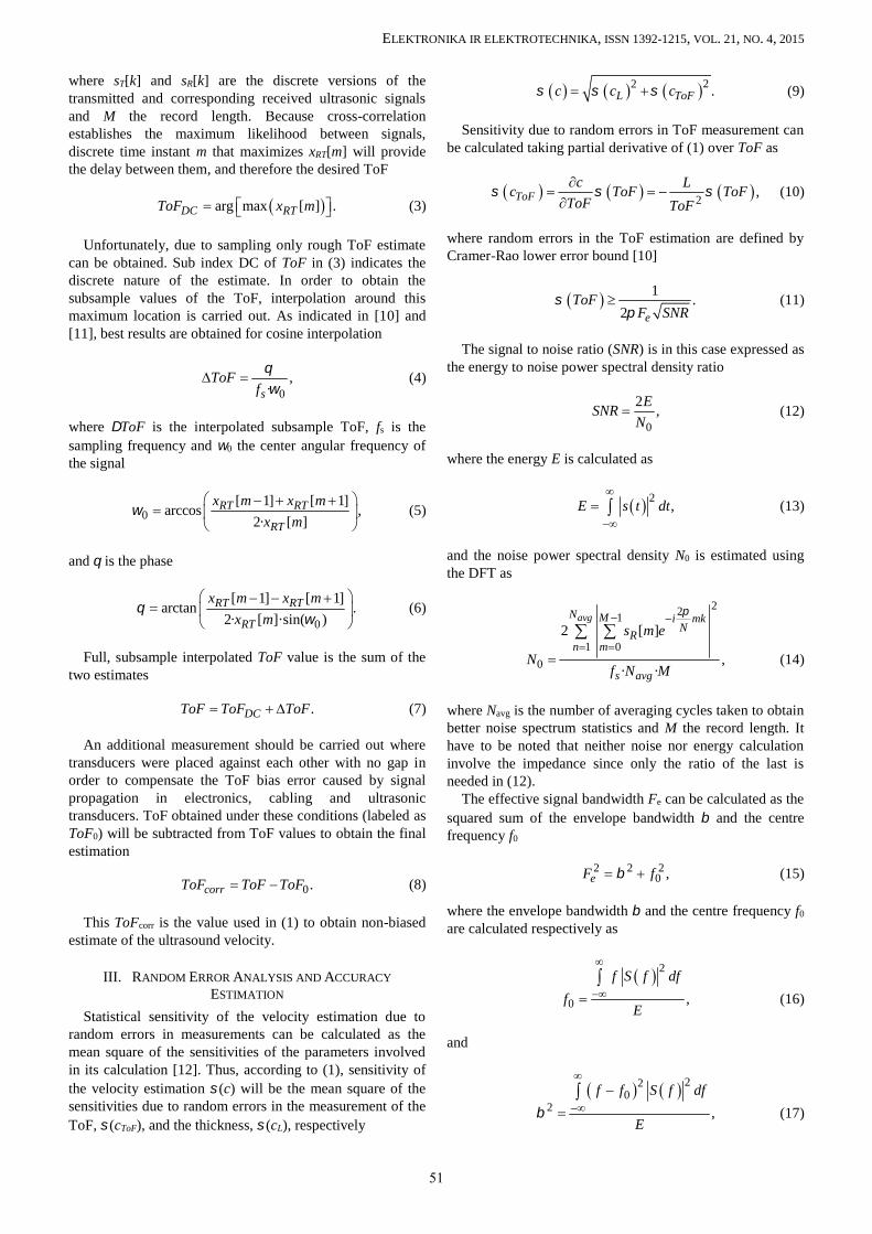
random error obtained using (11) is shown in Fig. 9.

0 24 48 72 96 120 1440.0

10.0p

20.0p

30.0p

40.0p

50.0p

60.0p

70.0p

Chirp 0.7-3.5MHz

Chirp 0.5-5MHz

CW toneburst

Pulse

Pulse CW toneburst Chirp 0.5-5MHz Chirp 0.7-3.5MHz(

ToF)

(s)

Time (h)Fig. 9. Theoretical random errors of the ToF estimation obtained frommeasured system parameters.

Taking the envelope bandwidth = 1.8 MHz andsampling frequency fs = 100 MHz, the resulting maximumvalue of the interpolation error (ToFss) according to (20) is5.5 ps. Comparing this value with the results shown in Fig. 9(10 ps minimum) it can be concluded that interpolationerrors can be neglected.

Figure 9 also shows that the lowest random errors areexpected for wideband chirp (0.5 MHz to 5 MHz), whileworst performance is expected for the pulse signal (becauseof the lower energy). On the other hand, a significantdisadvantage can be seen for CW toneburst signal: there areabrupt ToF estimation errors, which are caused by peaklocation on neighbouring CW period.

Random errors of the time scale can be neglected takinginto account that reference clock oscillator (ASEMPC) have3 ps jitter. Time scale bias errors are defined by initialfrequency stability of the oscillator (10 ppm), oscillatorageing (5 ppm/year) and the ToF being measured. Assuming15 ps as standard deviation for the time scale bias error (1year of exploitation) and taking ToF values from theexperiment, the expected velocity estimation bias errors areshown in Fig. 10.

0 20 40 60 80 100 120 14025.0p

30.0p

35.0p

40.0p

45.0p

(To

F) (s

)

Time (h)Fig. 10. Theoretical random errors of the ToF estimation caused by timescale bias.

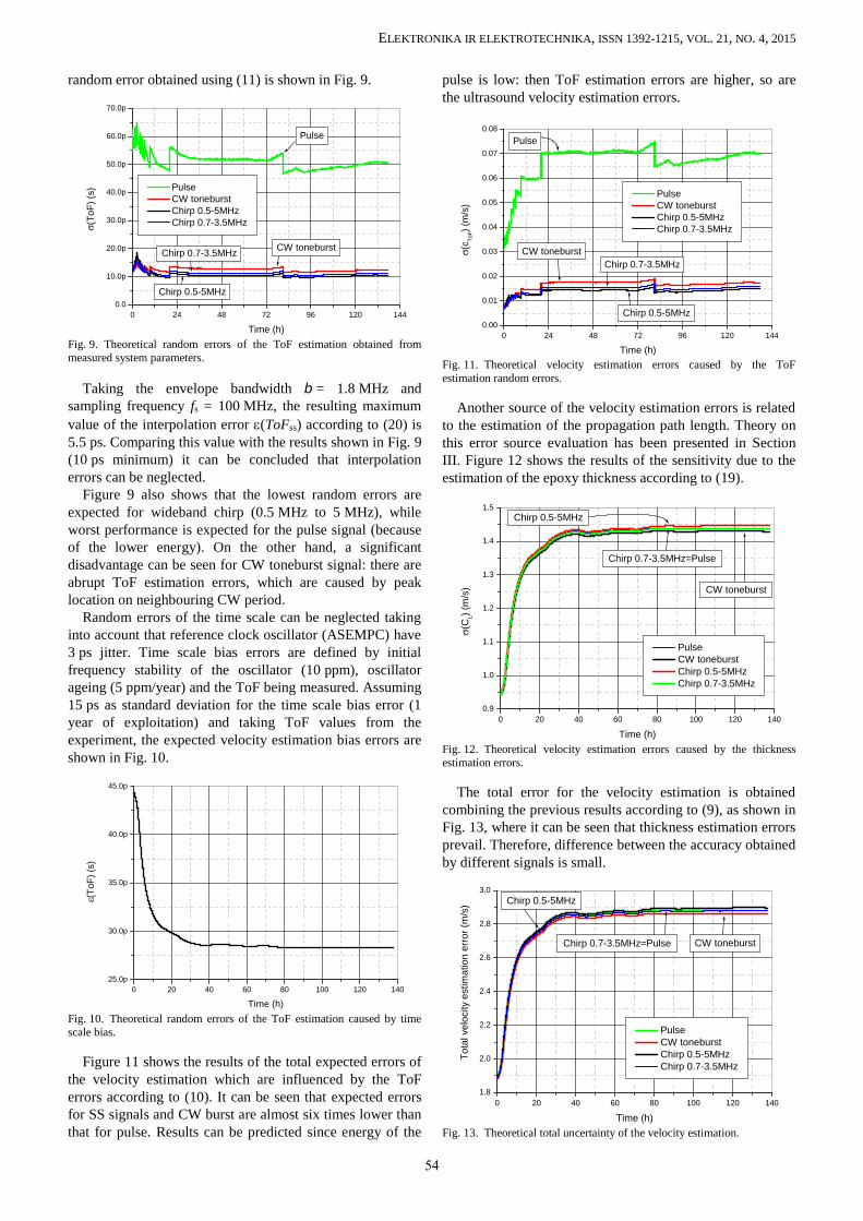
Figure 11 shows the results of the total expected errors ofthe velocity estimation which are influenced by the ToFerrors according to (10). It can be seen that expected errorsfor SS signals and CW burst are almost six times lower thanthat for pulse. Results can be predicted since energy of the

pulse is low: then ToF estimation errors are higher, so arethe ultrasound velocity estimation errors.

0 24 48 72 96 120 1440.00

0.01

0.02

0.03

0.04

0.05

0.06

0.07

0.08

Chirp 0.7-3.5MHz

Chirp 0.5-5MHz

CW toneburst

Pulse

Pulse CW toneburst Chirp 0.5-5MHz Chirp 0.7-3.5MHz

(c To

F) (m

/s)

Time (h)Fig. 11. Theoretical velocity estimation errors caused by the ToFestimation random errors.

Another source of the velocity estimation errors is relatedto the estimation of the propagation path length. Theory onthis error source evaluation has been presented in SectionIII. Figure 12 shows the results of the sensitivity due to theestimation of the epoxy thickness according to (19).

0 20 40 60 80 100 120 1400.9

1.0

1.1

1.2

1.3

1.4

1.5

CW toneburst

Chirp 0.5-5MHz

Chirp 0.7-3.5MHz=Pulse

Pulse CW toneburst Chirp 0.5-5MHz Chirp 0.7-3.5MHz

(C

L) (m

/s)

Time (h)Fig. 12. Theoretical velocity estimation errors caused by the thicknessestimation errors.

The total error for the velocity estimation is obtainedcombining the previous results according to (9), as shown inFig. 13, where it can be seen that thickness estimation errorsprevail. Therefore, difference between the accuracy obtainedby different signals is small.

0 20 40 60 80 100 120 1401.8

2.0

2.2

2.4

2.6

2.8

3.0Chirp 0.5-5MHz

CW toneburstChirp 0.7-3.5MHz=Pulse

Pulse CW toneburst Chirp 0.5-5MHz Chirp 0.7-3.5MHz

Tota

l vel

ocity

est

imat

ion

erro

r (m

/s)

Time (h)Fig. 13. Theoretical total uncertainty of the velocity estimation.

54

ELEKTRONIKA IR ELEKTROTECHNIKA, ISSN 1392-1215, VOL. 21, NO. 4, 2015

Finally, Fig. 14 shows the velocity values for the end ofcuring with its confidence interval. It can be seen that errorsobtained by theoretical analysis, using measured systemparameters, are low enough to give the confidence inchemical process monitoring.

24 48 72 96 120 240 2642560

2580

2600

2620

2640

2660

2680

2700

2720

2740

95% confidence interval

After accelerated temperature cure

After 10 days

Ultr

asou

nd v

eloc

ity (m

/s)

Time (h)Fig. 14. Measured velocity for curing end with confidence interval shown.

Value of this research lies in the evaluation of the errorsand comparison between different signal types. Future studyshould account other sources of errors (such as transducersattachment or temperature) so these are handled properly toreliably indicate the process stage.

VI. CONCLUSIONS

In this study, the assessment of the chemical processmonitoring using the ultrasound velocity has been carriedout. The results indicate that time of flight estimation errorsare strongly influenced by the signal energy. The lowesterrors are obtained for wideband chirp, so its use isrecommended to improve the accuracy and reliability of themonitoring process. The worst performance, due to lowenergy, is for the pulse signal. CW toneburst has asignificant disadvantage: abrupt ToF estimation errors occurare caused by peak location on neighbouring CW periodeven at significant SNR level.

On the other hand, the difference in accuracy between thesignals is small because thickness estimation errors prevailin the final error budget. This study indicates also that theuncertainty in the velocity estimation due to the parametersof the measurement system is low enough to ensure theconfidence in the chemical process monitoring.

Further study is needed to assure that other sources oferrors are handled properly to reliably predict the end ofchemical curing process, especially those concerning the

transducers attachment and the temperature monitoring.

REFERENCES

[1] W. Stark, H. Goering, U. Michel, H. Bayerl, “Online monitoring ofthermoset postcuring by dynamic mechanical thermal analysis”, inProc. DMTA. Polym. Test., vol. 28, pp. 561–566, 2009. [Online].Available: http://dx.doi.org/10.1016/j.polymertesting.2009.02.005

[2] F. Lionetto, A. Maffezzoli, “Monitoring the cure state ofthermosetting resins by ultrasound”, Materials, vol. 6, pp. 3783–3804,2013. [Online] Available: http://dx.doi.org/10.3390/ma6093783

[3] A. G. Mamalis, N. G. Pantelelis, K. N. Spentzas, “Process monitoringand cure control applied in RTM production of epoxy/carbon fibreparts”, in Proc. TMS-ABM International Materials Congress, Rio deJaneiro, Brazil, 2010, pp. 4568–4576.

[4] N. Liebers, F. Raddatz, F. Schadow, “Effective and flexibleultrasound sensors for cure monitoring for industrial compositeproduction”, Deutsche Gesellschaft für Luft- und Raumfahrt -Lilienthal-Oberth e.V., pp. 1–6, 2012.

[5] P. J. Schubel, R. J. Crossley, E. K. G. Boateng, J. R. Hutchinson,“Review of structural health and cure monitoring techniques for largewind turbine blades”, Renewable Energy, vol. 51, pp. 113–123, 2013.[Online] Available: http://dx.doi.org/10.1016/j.renene.2012.08.072

[6] V. Samaitis, L. Mazeika, “Investigation of diffuse LambWaveSensitivity to the Through-Thickness Notch in Structural Healthmonitoring of composite objects”, Elektronika Ir Elektrotechnika,vol. 20, no. 3, pp. 48–51, 2014. [Online] Available:http://dx.doi.org/10.5755/j01.eee.20.3.6690

[7] Z Luo, H. Zhu, J. Zhao, “In Situ monitoring of epoxy resin curingprocess using ultrasonic technique”, Experimental Techniques,vol. 36, no. 2, pp. 6–11, 2012. [Online] Available:http://onlinelibrary.wiley.com/doi/10.1111/j.1747-1567.2011.00741.x/full

[8] L. Svilainis, V. Dumbrava, S. Kitov, A. Aleksandrovas, P. Tervydis,D. Liaukonis, “Electronics for ultrasonic imaging system”,Elektronika Ir Elektrotechnika, vol. 20, no. 7, pp. 51–56, 2014.[Online] Available: http://dx.doi.org/10.5755/j01.eee.20.7.8024

[9] M. R. Hoseini, X. Wang, M. J. Zuo, “Estimating ultrasonic time offlight using envelope and quasi maximum likelihood method fordamage detection and assessment”, Measurement, vol. 45, pp. 2072–2080, 2012. [Online] Available:http://dx.doi.org/10.1016/j.measurement.2012.05.008

[10] L. Svilainis, K. Lukoseviciute, V. Dumbrava, A. Chaziachmetovas,“Subsample interpolation bias error in time of flight estimation bydirect correlation in digital domain”, Measurement, vol. 46, pp. 3950–3958, 2013. [Online] Available:http://dx.doi.org/10.1016/j.measurement.2013.07.038

[11] I. Cespedes, Y. Huang, J. Ophir, S. Spratt, “Methods for estimation ofsubsample time delays of digitized echo signals”, Ultrasonic Imaging,vol. 17, pp. 142–171, 1995. [Online] Available:http://uix.sagepub.com/content/17/2/142.reprint

[12] Expression of the Uncertainty of Measurement in Calibration, EA-4/02, European cooperation for accreditation, 1999. [Online]Available: http://www.european-accreditation.org/publication/ea-4-02-m

[13] L. Svilainis et al., “Acquisition system for the arbitrary pulse widthand position signals application in ultrasound”, Sensor Letters,vol. 12, no. 9, pp. 1399–1407, 2014. [Online] Available:http://dx.doi.org/10.1166/sl.2014.3329

[14] C. E. Corcione, F. Freuli, M. Frigione, “Cold-curing structural epoxyresins: analysis of the curing reaction as a function of curing time andthickness”, Materials, vol. 7, pp. 6832–6842, 2014. [Online]Available: http://www.mdpi.com/1996-1944/7/9/6832

55