91
Asymptotic Analysis and Singular Perturbation Theory John K. Hunter Department of Mathematics University of California at Davis February, 2004 Copyright c 2004 John K. Hunter

Asymptotic Analysis andSingular Perturbation Theory
John K. Hunter
Department of MathematicsUniversity of California at Davis
February, 2004
Copyright c© 2004 John K. Hunter

ii
Contents
Chapter 1 Introduction 11.1 Perturbation theory . . . . . . . . . . . . . . . . . . . . . . . . . . . . 1
1.1.1 Asymptotic solutions . . . . . . . . . . . . . . . . . . . . . . . . . 11.1.2 Regular and singular perturbation problems . . . . . . . . . . . . 2
1.2 Algebraic equations . . . . . . . . . . . . . . . . . . . . . . . . . . . . . 31.3 Eigenvalue problems . . . . . . . . . . . . . . . . . . . . . . . . . . . . 7
1.3.1 Quantum mechanics . . . . . . . . . . . . . . . . . . . . . . . . . 91.4 Nondimensionalization . . . . . . . . . . . . . . . . . . . . . . . . . . . 12
Chapter 2 Asymptotic Expansions 192.1 Order notation . . . . . . . . . . . . . . . . . . . . . . . . . . . . . . . 192.2 Asymptotic expansions . . . . . . . . . . . . . . . . . . . . . . . . . . . 20
2.2.1 Asymptotic power series . . . . . . . . . . . . . . . . . . . . . . . 212.2.2 Asymptotic versus convergent series . . . . . . . . . . . . . . . . 232.2.3 Generalized asymptotic expansions . . . . . . . . . . . . . . . . . 252.2.4 Nonuniform asymptotic expansions . . . . . . . . . . . . . . . . . 27
2.3 Stokes phenomenon . . . . . . . . . . . . . . . . . . . . . . . . . . . . . 27
Chapter 3 Asymptotic Expansion of Integrals 293.1 Euler’s integral . . . . . . . . . . . . . . . . . . . . . . . . . . . . . . . 293.2 Perturbed Gaussian integrals . . . . . . . . . . . . . . . . . . . . . . . 323.3 The method of stationary phase . . . . . . . . . . . . . . . . . . . . . . 353.4 Airy functions and degenerate stationary phase points . . . . . . . . . 37
3.4.1 Dispersive wave propagation . . . . . . . . . . . . . . . . . . . . 403.5 Laplace’s Method . . . . . . . . . . . . . . . . . . . . . . . . . . . . . . 43
3.5.1 Multiple integrals . . . . . . . . . . . . . . . . . . . . . . . . . . 453.6 The method of steepest descents . . . . . . . . . . . . . . . . . . . . . 46
Chapter 4 The Method of Matched Asymptotic Expansions: ODEs 494.1 Enzyme kinetics . . . . . . . . . . . . . . . . . . . . . . . . . . . . . . 49
iii

4.1.1 Outer solution . . . . . . . . . . . . . . . . . . . . . . . . . . . . 514.1.2 Inner solution . . . . . . . . . . . . . . . . . . . . . . . . . . . . . 524.1.3 Matching . . . . . . . . . . . . . . . . . . . . . . . . . . . . . . . 53
4.2 General initial layer problems . . . . . . . . . . . . . . . . . . . . . . . 544.3 Boundary layer problems . . . . . . . . . . . . . . . . . . . . . . . . . 55
4.3.1 Exact solution . . . . . . . . . . . . . . . . . . . . . . . . . . . . 554.3.2 Outer expansion . . . . . . . . . . . . . . . . . . . . . . . . . . . 564.3.3 Inner expansion . . . . . . . . . . . . . . . . . . . . . . . . . . . 574.3.4 Matching . . . . . . . . . . . . . . . . . . . . . . . . . . . . . . . 584.3.5 Uniform solution . . . . . . . . . . . . . . . . . . . . . . . . . . . 584.3.6 Why is the boundary layer at x = 0? . . . . . . . . . . . . . . . . 59
4.4 Boundary layer problems for linear ODEs . . . . . . . . . . . . . . . . 594.5 A boundary layer problem for capillary tubes . . . . . . . . . . . . . . 63
4.5.1 Formulation . . . . . . . . . . . . . . . . . . . . . . . . . . . . . . 634.5.2 Wide circular tubes . . . . . . . . . . . . . . . . . . . . . . . . . 65
Chapter 5 Method of Multiple Scales: ODEs 735.1 Periodic solutions and the Poincare-Lindstedt expansion . . . . . . . . 73
5.1.1 Duffing’s equation . . . . . . . . . . . . . . . . . . . . . . . . . . 735.1.2 Van der Pol oscillator . . . . . . . . . . . . . . . . . . . . . . . . 77
5.2 The method of multiple scales . . . . . . . . . . . . . . . . . . . . . . . 785.3 The method of averaging . . . . . . . . . . . . . . . . . . . . . . . . . . 795.4 Perturbations of completely integrable Hamiltonian systems . . . . . . 825.5 The WKB method for ODEs . . . . . . . . . . . . . . . . . . . . . . . 83
Bibliography 87
iv

Chapter 1
Introduction
In this chapter, we describe the aims of perturbation theory in general terms, andgive some simple illustrative examples of perturbation problems. Some texts andreferences on perturbation theory are [8], [9], and [13].
1.1 Perturbation theory
Consider a problem
P ε(x) = 0 (1.1)
depending on a small, real-valued parameter ε that simplifies in some way whenε = 0 (for example, it is linear or exactly solvable). The aim of perturbation theoryis to determine the behavior of the solution x = xε of (1.1) as ε→ 0. The use of asmall parameter here is simply for definiteness; for example, a problem dependingon a large parameter ω can be rewritten as one depending on a small parameterε = 1/ω.
The focus of these notes is on perturbation problems involving differential equa-tions, but perturbation theory and asymptotic analysis apply to a broad class ofproblems. In some cases, we may have an explicit expression for xε, such as anintegral representation, and want to obtain its behavior in the limit ε→ 0.
1.1.1 Asymptotic solutions
The first goal of perturbation theory is to construct a formal asymptotic solution of(1.1) that satisfies the equation up to a small error. For example, for each N ∈ N,we may be able to find an asymptotic solution xεN such that
P ε (xεN ) = O(εN+1),
where O(εn) denotes a term of the the order εn. This notation will be made precisein Chapter 2.
1

Once we have constructed such an asymptotic solution, we would like to knowthat there is an exact solution x = xε of (1.1) that is close to the asymptotic solutionwhen ε is small; for example, a solution such that
xε = xεN +O(εN+1).
This is the case if a small error in the equation leads to a small error in the solution.For example, we can establish such a result if we have a stability estimate of theform
|x− y| ≤ C |P ε(x)− P ε(y)|
where C is a constant independent of ε, and | · | denotes appropriate norms. Such anestimate depends on the properties of P ε and may be difficult to obtain, especiallyfor nonlinear problems. In these notes we will focus on methods for the constructionof asymptotic solutions, and we will not discuss in detail the existence of solutionsclose to the asymptotic solution.
1.1.2 Regular and singular perturbation problems
It is useful to make an imprecise distinction between regular perturbation problemsand singular perturbation problems. A regular perturbation problem is one for whichthe perturbed problem for small, nonzero values of ε is qualitatively the same asthe unperturbed problem for ε = 0. One typically obtains a convergent expansionof the solution with respect to ε, consisting of the unperturbed solution and higher-order corrections. A singular perturbation problem is one for which the perturbedproblem is qualitatively different from the unperturbed problem. One typicallyobtains an asymptotic, but possibly divergent, expansion of the solution, whichdepends singularly on the parameter ε.
Although singular perturbation problems may appear atypical, they are the mostinteresting problems to study because they allow one to understand qualitativelynew phenomena.
The solutions of singular perturbation problems involving differential equationsoften depend on several widely different length or time scales. Such problems canbe divided into two broad classes: layer problems, treated using the method ofmatched asymptotic expansions (MMAE); and multiple-scale problems, treated bythe method of multiple scales (MMS). Prandtl’s boundary layer theory for the high-Reynolds flow of a viscous fluid over a solid body is an example of a boundary layerproblem, and the semi-classical limit of quantum mechanics is an example of amultiple-scale problem.
We will begin by illustrating some basic issues in perturbation theory with simplealgebraic equations.
2

1.2 Algebraic equations
The first two examples illustrate the distinction between regular and singular per-turbation problems.
Example 1.1 Consider the cubic equation
x3 − x+ ε = 0. (1.2)
We look for a solution of the form
x = x0 + εx1 + ε2x2 +O(ε3). (1.3)
Using this expansion in the equation, expanding, and equating coefficients of εn tozero, we get
x30 − x0 = 0,
3x20x1 − x1 + 1 = 0,
3x0x2 − x2 + 3x0x21 = 0.
Note that we obtain a nonlinear equation for the leading order solution x0, andnonhomogeneous linearized equations for the higher order corrections x1, x2,. . . .This structure is typical of many perturbation problems.
Solving the leading-order perturbation equation, we obtain the three roots
x0 = 0,±1.
Solving the first-order perturbation equation, we find that
x1 =1
1− 3x20
.
The corresponding solutions are
x = ε+O(ε2), x = ±1− 12ε+O(ε2).
Continuing in this way, we can obtain a convergent power series expansion aboutε = 0 for each of the three distinct roots of (1.2). This result is typical of regularperturbation problems.
An alternative — but equivalent — method to obtain the perturbation series isto use the Taylor expansion
x(ε) = x(0) + x(0)ε+12!x(0)ε2 + . . . ,
where the dot denotes a derivative with respect to ε. To compute the coefficients,we repeatedly differentiate the equation with respect to ε and set ε = 0 in the result.
3

For example, setting ε = 0 in (1.2), and solving the resulting equation for x(0), weget x(0) = 0,±1. Differentiating (1.2) with respect to ε, we get
3x2x− x+ 1 = 0.
Setting ε = 0 and solving for x(0), we get the same answer as before.
Example 1.2 Consider the cubic equation
εx3 − x+ 1 = 0. (1.4)
Using (1.3) in (1.4), expanding, and equating coefficents of εn to zero, we get
−x0 + 1 = 0,
−x1 + x30 = 0,
−x2 + 3x20x1 = 0.
Solving these equations, we find that x0 = 1, x1 = 1, . . . , and hence
x(ε) = 1 + ε+O(ε2). (1.5)
We only obtain one solution because the cubic equation (1.4) degenerates to a linearequation at ε = 0. We missed the other two solutions because they approach infinityas ε → 0. A change in the qualitative nature of the problem at the unperturbedvalue ε = 0 is typical of singular perturbation problems.
To find the other solutions, we introduce a rescaled variable y, where
x(ε) =1δ(ε)
y(ε),
and y = O(1) as ε → 0. The scaling factor δ is to be determined. Using thisequation in (1.4), we find that
ε
δ3y3 − 1
δy + 1 = 0. (1.6)
In order to obtain a nontrivial solution, we require that at least two leading-orderterms in this equation have the same order of magnitude. This is called the principleof dominant balance.
Balancing the first two terms, we find that∗
ε
δ3=
1δ,
which implies that δ = ε1/2. The first two terms in (1.4) are then O(ε−1/2), and thethird term is O(1), which is smaller. With this choice of δ, equation (1.6) becomes
y3 − y + ε1/2 = 0.
∗Nonzero constant factors can be absorbed into y.
4

Solving this equation in the same way as (1.2), we get the nonzero solutions
y = ±1− 12ε1/2 +O(ε).
The corresponding solutions for x are
x = ± 1ε1/2
− 12
+O(ε1/2
).
The dominant balance argument illustrated here is useful in many perturbationproblems. The corresponding limit, ε→ 0 with x(ε) = O(ε−1/2), is called a distin-guished limit.
There are two other two-term balances in (1.6). Balancing the second and thirdterms, we find that
1δ
= 1
or δ = 1. The first term is then O(ε), so it is smaller than the other two terms. Thisdominant balance gives the solution in (1.5). Balancing the first and third terms,we find that
ε
δ3= 1,
or δ = ε1/3. In this case, the first and third terms are O(1), but the second termis O(ε−1/3). Thus, it is larger than the terms that balance, so we do not obtain adominant balance or any new solutions.
In this example, no three-term dominant balance is possible as ε → 0, but thiscan occur in other problems.
Example 1.3 A famous example of the effect of a perturbation on the solutions ofa polynomial is Wilkinson’s polynomial (1964),
(x− 1)(x− 2) . . . (x− 20) = εx19.
The perturbation has a large effect on the roots even for small values of ε.
The next two examples illustrate some other features of perturbation theory.
Example 1.4 Consider the quadratic equation
(1− ε)x2 − 2x+ 1 = 0.
Suppose we look for a straightforward power series expansion of the form
x = x0 + εx1 +O(ε2).
We find that
x20 − 2x0 + 1 = 0,
2(x0 − 1)x1 = x20.
5

Solving the first equation, we get x0 = 1. The second equation then becomes 0 = 1.It follows that there is no solution of the assumed form.
This difficulty arises because x = 1 is a repeated root of the unperturbed prob-lem. As a result, the solution
x =1± ε1/2
1− ε
does not have a power series expansion in ε, but depends on ε1/2. An expansion
x = x0 + ε1/2x1 + εx2 +O(ε3/2)
leads to the equations x0 = 1, x21 = 1, or
x = 1± ε1/2 +O(ε)
in agreement with the exact solution.
Example 1.5 Consider the transcendental equation
xe−x = ε. (1.7)
As ε→ 0+, there are two possibilities:
(a) x→ 0, which implies that x = ε+ ε2 +O(ε2);(b) e−x → 0, when x→∞.
In the second case, x must be close to log 1/ε.To obtain an asymptotic expansion for the solution, we solve the equation itera-
tively using the idea that e−x varies much more rapidly than x as x→ 0. Rewriting(1.7) as e−x = ε/x and taking logarithms, we get the equivalent equation
x = log x+ log1ε.
Thus solutions are fixed points of the function
f(x) = log x+ log1ε.
We then define iterates xn, n ∈ N, by
xn+1 = log xn + log1ε,
x1 = log1ε.
Defining
L1 = log1ε, L2 = log
(log
1ε
),
6

we find that
x2 = L1 + L2,
x3 = L1 + log(L1 + L2)
= L1 + L2 +L2
L1+O
((L2
L1
)2).
At higher orders, terms involving
L3 = log(
log(
log1ε
)),
and so on, appear.The form of this expansion would be difficult to guess without using an iterative
method. Note, however, that the successive terms in this asymptotic expansionconverge very slowly as ε → 0. For example, although L2/L1 → 0 as ε → 0, whenε = 0.1, L1 ≈ 36, L2 ≈ 12; and when ε = 10−5, L1 ≈ 19, L2 ≈ 1.
1.3 Eigenvalue problems
Spectral perturbation theory studies how the spectrum of an operator is perturbedwhen the operator is perturbed. In general, this question is a difficult one, andsubtle phenomena may occur, especially in connection with the behavior of thecontinuous spectrum of the operators. Here, we consider the simplest case of theperturbation in an eigenvalue.
Let H be a Hilbert space with inner product 〈·, ·〉, and Aε : D(Aε) ⊂ H → H alinear operator in H, with domain D(Aε), depending smoothly on a real parameterε. We assume that:
(a) Aε is self-adjoint, so that
〈x,Aεy〉 = 〈Aεx, y〉 for all x, y ∈ D(Aε);
(b) Aε has a smooth branch of simple eigenvalues λε ∈ R with eigenvectorsxε ∈ H, meaning that
Aεxε = λεxε. (1.8)
We will compute the perturbation in the eigenvalue from its value at ε = 0 when ε
is small but nonzero.A concrete example is the perturbation in the eigenvalues of a symmetric matrix.
In that case, we have H = Rn with the Euclidean inner product
〈x, y〉 = xT y,
7

and Aε : Rn → Rn is a linear transformation with an n×n symmetric matrix (aεij).The perturbation in the eigenvalues of a Hermitian matrix corresponds to H = Cnwith inner product 〈x, y〉 = xT y. As we illustrate below with the Schrodingerequation of quantum mechanics, spectral problems for differential equations can beformulated in terms of unbounded operators acting in infinite-dimensional Hilbertspaces.
We use the expansions
Aε = A0 + εA1 + . . .+ εnAn + . . . ,
xε = x0 + εx1 + . . .+ εnxn + . . . ,
λε = λ0 + ελ1 + . . .+ εnλn + . . .
in the eigenvalue problem (1.8), equate coefficients of εn, and rearrange the result.We find that
(A0 − λ0I)x0 = 0, (1.9)
(A0 − λ0I)x1 = −A1x0 + λ1x0, (1.10)
(A0 − λ0I)xn =n∑i=1
−Aixn−i + λixn−i . (1.11)
Assuming that x0 6= 0, equation (1.9) implies that λ0 is an eigenvalue of A0
and x0 is an eigenvector. Equation (1.10) is then a singular equation for x1. Thefollowing proposition gives a simple, but fundamental, solvability condition for thisequation.
Proposition 1.6 Suppose that A is a self-adjoint operator acting in a Hilbert spaceH and λ ∈ R. If z ∈ H, a necessary condition for the existence of a solution y ∈ Hof the equation
(A− λI) y = z (1.12)
is that
〈x, z〉 = 0,
for every eigenvector x of A with eigenvalue λ.
Proof. Suppose z ∈ H and y is a solution of (1.12). If x is an eigenvector of A,then using (1.12) and the self-adjointness of A− λI, we find that
〈x, z〉 = 〈x, (A− λI) y〉= 〈(A− λI)x, y〉= 0.
8

In many cases, the necesary solvability condition in this proposition is also suf-ficient, and then we say that A−λI satisfies the Fredholm alternative; for example,this is true in the finite-dimensional case, or when A is an elliptic partial differentialoperator.
SinceA0 is self-adjoint and λ0 is a simple eigenvalue with eigenvector x0, equation(1.12) it is solvable for x1 only if the right hand side is orthogonal to x0, which im-plies that
λ1 =〈x0, A1x0〉〈x0, x0〉
.
This equation gives the leading order perturbation in the eigenvalue, and is themost important result of the expansion.
Assuming that the necessary solvability condition in the proposition is sufficient,we can then solve (1.10) for x1. A solution for x1 is not unique, since we can addto it an arbitrary scalar multiple of x0. This nonuniqueness is a consequence of thefact that if xε is an eigenvector of Aε, then cεxε is also a solution for any scalar cε.If
cε = 1 + εc1 +O(ε2)
then
cεxε = x0 + ε (x1 + c1x0) +O(ε2).
Thus, the addition of c1x0 to x1 corresponds to a rescaling of the eigenvector by afactor that is close to one.
This expansion can be continued to any order. The solvability condition for(1.11) determines λn, and the equation may then be solved for xn, up to an arbitraryvector cnx0. The appearance of singular problems, and the need to impose solvabiltyconditions at each order which determine parameters in the expansion and allow forthe solution of higher order corrections, is a typical structure of many pertubationproblems.
1.3.1 Quantum mechanics
One application of this expansion is in quantum mechanics, where it can be usedto compute the change in the energy levels of a system caused by a perturbation inits Hamiltonian.
The Schrodinger equation of quantum mechanics is
i~ψt = Hψ.
Here t denotes time and ~ is Planck’s constant. The wavefunction ψ(t) takes valuesin a Hilbert space H, and H is a self-adjoint linear operator acting in H with thedimensions of energy, called the Hamiltonian.
9

Energy eigenstates are wavefunctions of the form
ψ(t) = e−iEt/~ϕ,
where ϕ ∈ H and E ∈ R. It follows from the Schrodinger equation that
Hϕ = Eϕ.
Hence E is an eigenvalue of H and ϕ is an eigenvector. One of Schrodinger’smotivations for introducing his equation was that eigenvalue problems led to theexperimentally observed discrete energy levels of atoms.
Now suppose that the Hamiltonian
Hε = H0 + εH1 +O(ε2)
depends smoothly on a parameter ε. Then, rewriting the previous result, we findthat the corresponding simple energy eigenvalues (assuming they exist) have theexpansion
Eε = E0 + ε〈ϕ0, H1ϕ0〉〈ϕ0, ϕ0〉
+O(ε2)
where ϕ0 is an eigenvector of H0.For example, the Schrodinger equation that describes a particle of mass m mov-
ing in Rd under the influence of a conservative force field with potential V : Rd → Ris
i~ψt = − ~2
2m∆ψ + V ψ.
Here, the wavefunction ψ(x, t) is a function of a space variable x ∈ Rd and timet ∈ R. At fixed time t, we have ψ(·, t) ∈ L2(Rd), where
L2(Rd) =u : Rd → C | u is measurable and
∫Rd |u|2 dx <∞
is the Hilbert space of square-integrable functions with inner-product
〈u, v〉 =∫
Rd
u(x)v(x) dx.
The Hamiltonian operator H : D(H) ⊂ H → H, with domain D(H), is given by
H = − ~2
2m∆ + V.
If u, v are smooth functions that decay sufficiently rapidly at infinity, then Green’stheorem implies that
〈u,Hv〉 =∫
Rd
u
(− ~2
2m∆v + V v
)dx
=∫
Rd
~2
2m∇ · (v∇u− u∇v)− ~2
2m(∆u)v + V uv
dx
10

=∫
Rd
(− ~2
2m∆u+ V u
)v dx
= 〈Hu, v〉.
Thus, this operator is formally self-adjoint. Under suitable conditions on the poten-tial V , the operator can be shown to be self-adjoint with respect to an appropriatelychosen domain.
Now suppose that the potential V ε depends on a parameter ε, and has theexpansion
V ε(x) = V0(x) + εV1(x) +O(ε2).
The perturbation in a simple energy eigenvalue
Eε = E0 + εE1 +O(ε2),
assuming one exists, is given by
E1 =
∫Rd V1(x)|ϕ0(x)|2 dx∫
Rd |ϕ0(x)|2 dx,
where ϕ0 ∈ L2(Rd) is an unperturbed energy eigenfunction that satisfies
− ~2
2m∆ϕ0 + V0ϕ0 = E0ϕ0.
Example 1.7 The one-dimensional simple harmonic oscillator has potential
V0(x) =12kx2.
The eigenvalue problem
− ~2
2mϕ′′ +
12kx2ϕ = Eϕ, ϕ ∈ L2(R)
is exactly solvable. The energy eigenvalues are
En = ~ω(n+
12
)n = 0, 1, 2, . . . ,
where
ω =
√k
m
is the frequency of the corresponding classical oscillator. The eigenfunctions are
ϕn(x) = Hn(αx)e−α2x2/2,
where Hn is the nth Hermite polynomial,
Hn(ξ) = (−1)neξ2 dn
dξne−ξ
2,
11

and the constant α, with dimensions of 1/length, is given by
α2 =
√mk
~.
The energy levels Eεn of a slightly anharmonic oscillator with potential
V ε(x) =12kx2 + ε
k
α2W (αx) +O(ε2) as ε→ 0+
where ε > 0 have the asymptotic behavior
Eεn = ~ωn+
12
+ ε∆n +O(ε2)
as ε→ 0+,
where
∆n =∫W (ξ)H2
n(ξ)e−ξ2dξ∫
H2n(ξ)e−ξ2 dξ
.
For an extensive and rigorous discussion of spectral perturbation theory forlinear operators, see [11].
1.4 Nondimensionalization
The numerical value of any quantity in a mathematical model is measured withrespect to a system of units (for example, meters in a mechanical model, or dollarsin a financial model). The units used to measure a quantity are arbitrary, and achange in the system of units (for example, to feet or yen, at a fixed exchange rate)cannot change the predictions of the model. A change in units leads to a rescalingof the quantities. Thus, the independence of the model from the system of unitscorresponds to a scaling invariance of the model. In cases when the zero point of aunit is arbitrary, we also obtain a translational invariance, but we will not considertranslational invariances here.
Suppose that a model involves quantities (a1, a2, . . . , an), which may include de-pendent and independent variables as well as parameters. We denote the dimensionof a quantity a by [a]. A fundamental system of units is a minimal set of indepen-dent units, which we denote symbolically by (d1, d2, . . . , dr). Different fundamentalsystem of units can be used, but given a fundamental system of units any other de-rived unit may be constructed uniquely as a product of powers of the fundamentalunits, so that
[a] = dα11 dα2
2 . . . dαrr (1.13)
for suitable exponents (α1, α2, . . . , αr).
Example 1.8 In mechanical problems, a fundamental set of units is d1 = mass,d2 = length, d3 = time, or d1 = M , d2 = L, d3 = T , for short. Then velocity
12

V = L/T and momentum P = ML/T are derived units. We could use insteadmomentum P , velocity V , and time T as a fundamental system of units, when massM = P/V and length L = V T are derived units. In problems involving heat flow, wemay introduce temperature (measured, for example, in degrees Kelvin) as anotherfundamental unit, and in problems involving electromagnetism, we may introducecurrent (measured, for example, in Amperes) as another fundamental unit.
The invariance of a model under the change in units dj 7→ λjdj implies that itis invariant under the scaling transformation
ai → λα1,i
1 λα2,i
2 . . . λαr,ir ai i = 1, . . . , n
for any λ1, . . . λr > 0, where
[ai] = dα1,i
1 dα2,i
2 . . . dαr,ir . (1.14)
Thus, if
a = f (a1, . . . , an)
is any relation between quantities in the model with the dimensions in (1.13) and(1.14), then f has the scaling property that
λα11 λα2
2 . . . λαrr f (a1, . . . , an) = f
(λα1,11 λ
α2,12 . . . λαr,1
r a1, . . . , λα1,n
1 λα2,n
2 . . . λαr,nr an
).
A particular consequence of the invariance of a model under a change of units isthat any two quantities which are equal must have the same dimensions. This factis often useful in finding the dimension of some quantity.
Example 1.9 According to Newton’s second law,
force = rate of change of momentum with respect to time.
Thus, if F denotes the dimension of force and P the dimension of momentum,then F = P/T . Since P = MV = ML/T , we conclude that F = ML/T 2 (ormass× acceleration).
Example 1.10 In fluid mechanics, the shear viscosity µ of a Newtonian fluid is theconstant of proportionality that relates the viscous stress tensor T to the velocitygradient ∇u:
T =12µ(∇u +∇uT
).
Stress has dimensions of force/area, so
[T ] =ML
T 2
1L2
=M
LT 2.
13

The velocity gradient ∇u has dimensions of velocity/length, so
[∇u] =L
T
1L
=1T.
Equating dimensions, we find that
[µ] =M
LT.
We can also write [µ] = (M/L3)(L2/T ). It follows that if ρ0 is the density of thefluid, and µ = ρ0ν, then
[ν] =L2
T.
Thus ν, which is called the kinematical viscosity, has the dimensions of diffusivity.Physically it is the diffusivity of momentum. For example, in time T , viscous effectslead to the diffusion of momentum over a length scale of the order
√νT .
At 20C, the kinematic viscosity of water is approximately 1 mm2/s. Thus, inone second, viscous effects diffuse the fluid momentum over a distance of the order1 mm.
Scaling invariance implies that we can reduce the number of quantities appear-ing in the problem by the introduction of dimensionless variables. Suppose that(a1, . . . , ar) are a set of (nonzero) quantities whose dimensions form a fundamentalsystem of units. We denote the remaining quantities in the model by (b1, . . . , bm),where r +m = n. Then for suitable exponents (β1,i, . . . , βr,i), the quantity
Πi =bi
aβ1,i
1 . . . aβr,ir
is dimensionless, meaning that it is invariant under the scaling transformationsinduced by changes in units. Such dimensionless quantities can often be interpretedas the ratio of two quantities of the same dimension appearing in the problem (suchas a ratio of lengths, times, diffusivities, and so on). Perturbation methods aretypically applicable when one or more of these dimensionless quantities is small orlarge.
Any relationship of the form
b = f(a1, . . . , ar, b1, . . . , bm)
is equivalent to a relation
Π = f(1, . . . , 1,Π1, . . . ,Πm).
Thus, the introduction of dimensionless quantities reduces the number of variablesin the problem by the number of fundamental units involved in the problem. Inmany cases, nondimensionalization leads to a reduction in the number of parametersin the problem to a minimal number of dimensionless parameters. In some cases,
14

one may be able to use dimensional arguments to obtain the form of self-similarsolutions.
Example 1.11 Consider the following IVP for the Green’s function of the heatequation in Rd:
ut = ν∆u,
u(x, 0) = Eδ(x).
Here δ is the delta-function. The dimensioned parameters in this problem are thediffusivity ν and the energy E of the point source. The only length and timesscales are those that come from the independent variables (x, t), so the solution isself-similar.
We have [u] = θ, where θ denotes temperature, and, since∫Rd
u(x, 0) dx = E,
we have [E] = θLd. Dimensional analysis and the rotational invariance of theLaplacian ∆ imply that
u(x, t) =E
(νt)d/2f
(|x|√νt
).
Using this expression for u(x, t) in the PDE, we get an ODE for f(ξ),
f ′′ +(ξ
2+d− 1ξ
)f ′ +
d
2f = 0.
We can rewrite this equation as a first-order ODE for f ′ + ξ2f ,(
f ′ +ξ
2f
)′+d− 1ξ
(f ′ +
ξ
2f
)= 0.
Solving this equation, we get
f ′ +ξ
2f =
b
ξd−1,
where b is a constant of integration. Solving for f , we get
f(ξ) = ae−ξ2/4 + be−ξ
2/4
∫e−ξ
2
ξd−1dξ,
where a s another constant of integration. In order for f to be integrable, we mustset b = 0. Then
u(x, t) =aE
(νt)d/2exp
(−|x|
2
4νt
).
15
Imposing the requirement that ∫Rd
u(x, t) dx = E,
and using the standard integral∫Rd
exp(−|x|
2
2c
)dx = (2πc)d/2 ,
we find that a = (4π)−d/2, and
u(x, t) =E
(4πνt)d/2exp
(−|x|
2
4νt
).
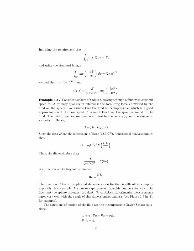
Example 1.12 Consider a sphere of radius L moving through a fluid with constantspeed U . A primary quantity of interest is the total drag force D exerted by thefluid on the sphere. We assume that the fluid is incompressible, which is a goodapproximation if the flow speed U is much less than the speed of sound in thefluid. The fluid properties are then determined by the density ρ0 and the kinematicviscosity ν. Hence,
D = f(U,L, ρ0, ν).
Since the drag D has the dimensions of force (ML/T 2), dimensional analysis impliesthat
D = ρ0U2L2F
(UL
ν
).
Thus, the dimensionless drag
D
ρ0U2L2= F (Re)
is a function of the Reynold’s number
Re =UL
ν.
The function F has a complicated dependence on Re that is difficult to computeexplicitly. For example, F changes rapidly near Reynolds numbers for which theflow past the sphere becomes turbulent. Nevertheless, experimental measurementsagree very well with the result of this dimensionless analysis (see Figure 1.9 in [1],for example).
The equations of motion of the fluid are the incompressible Navier-Stokes equa-tions,
ut + u · ∇u+∇p = ν∆u,
∇ · u = 0.
16

To nondimensionalize these equations with respect to (U,L, ρ), we introduce dimen-sionless variables
u∗ =u
U, p∗ =
p
ρU2, x∗ =
x
L, t∗ =
Ut
L,
and find that
u∗t∗ + u∗ · ∇∗u∗ +∇∗p∗ = ε∆∗u∗,
∇∗ · u∗ = 0.
Here,
ε =ν
UL=
1Re.
The boundary conditions correspond to a flow of speed 1 past a sphere of radius1. Thus, assuming that no other parameters enter into the problem, the dragcomputed from the solution of these equations depends only on ε, as obtained fromthe dimensional analysis above.
Dimensional analysis leads to continuous scaling symmetries. These scaling sym-metries are not the only continuous symmetries possessed by differential equations.The theory of Lie groups and Lie algebras provides a systematic method for com-puting all continuous symmetries of a given differential equation [18]. Lie originallyintroduced the notions of Lie groups and Lie algebras precisely for this purpose.
Example 1.13 The full group of symmetries of the one-dimensional heat equation
ut = uxx
is generated by the following transformations [18]:
u(x, t) 7→ u(x− α, t),u(x, t) 7→ u(x, t− β),
u(x, t) 7→ γu(x, t),
u(x, t) 7→ u(δx, δ2t),
u(x, t) 7→ e−εx+ε2tu(x− 2εt, t),
u(x, t) 7→ 1√1 + 4ηt
exp[−ηx2
1 + 4ηt
]u
(x
1 + 4ηt,
t
1 + 4ηt
),
u(x, t) 7→ u(x, t) + v(x, t),
where (α, . . . , η) are constants, and v(x, t) is an arbitrary solution of the heatequation. The scaling symmetries involving γ and δ can be deduced by dimen-sional arguments, but the symmetries involving ε and η cannot.
For further discussion of dimensional analysis and self-similar solutions, see [1].
17

18
Chapter 2
Asymptotic Expansions
In this chapter, we define the order notation and asymptotic expansions. For addi-tional discussion, see [4], and [17].
2.1 Order notation
The O and o order notation provides a precise mathematical formulation of ideasthat correspond — roughly — to the ‘same order of magnitude’ and ‘smaller orderof magnitude.’ We state the definitions for the asymptotic behavior of a real-valuedfunction f(x) as x → 0, where x is a real parameter. With obvious modifications,similar definitions apply to asymptotic behavior in the limits x → 0+, x → x0,x → ∞, to complex or integer parameters, and other cases. Also, by replacing | · |with a norm, we can define similiar concepts for functions taking values in a normedlinear space.
Definition 2.1 Let f, g : R \ 0→ R be real functions. We say f = O(g) as x→ 0if there are constants C and r > 0 such that
|f(x)| ≤ C|g(x)| whenever 0 < |x| < r.
We say f = o(g) as x→ 0 if for every δ > 0 there is an r > 0 such that
|f(x)| ≤ δ|g(x)| whenever 0 < |x| < r.
If g 6= 0, then f = O(g) as x→ 0 if and only if f/g is bounded in a (punctured)neighborhood of 0, and f = o(g) if and only if f/g → 0 as x→ 0.
We also write f g, or f is ‘much less than’ g, if f = o(g), and f ∼ g, or f isasymptotic to g, if f/g → 1.
Example 2.2 A few simple examples are:
(a) sin 1/x = O(1) as x→ 0
19
(b) it is not true that 1 = O(sin 1/x) as x → 0, because sin 1/x vanishes isevery neighborhood of x = 0;
(c) x3 = o(x2) as x→ 0, and x2 = o(x3) as x→∞;(d) x = o(log x) as x→ 0+, and log x = o(x) as x→∞;(e) sinx ∼ x as x→ 0;(f) e−1/x = o(xn) as x→ 0+ for any n ∈ N.
The o and O notations are not quantitative without estimates for the constantsC, δ, and r appearing in the definitions.
2.2 Asymptotic expansions
An asymptotic expansion describes the asymptotic behavior of a function in termsof a sequence of gauge functions. The definition was introduced by Poincare (1886),and it provides a solid mathematical foundation for the use of many divergent series.
Definition 2.3 A sequence of functions ϕn : R \ 0 → R, where n = 0, 1, 2, . . ., isan asymptotic sequence as x→ 0 if for each n = 0, 1, 2, . . . we have
ϕn+1 = o (ϕn) as x→ 0.
We call ϕn a gauge function. If ϕn is an asymptotic sequence and f : R \ 0→ Ris a function, we write
f(x) ∼∞∑n=0
anϕn(x) as x→ 0 (2.1)
if for each N = 0, 1, 2, . . . we have
f(x)−N∑n=0
anϕn(x) = o(ϕN ) as x→ 0.
We call (2.1) the asymptotic expansion of f with respect to ϕn as x→ 0.
Example 2.4 The functions ϕn(x) = xn form an asymptotic sequence as x→ 0+.Asymptotic expansions with respect to this sequence are called asymptotic powerseries, and they are discussed further below. The functions ϕn(x) = x−n form anasymptotic sequence as x→∞.
Example 2.5 The function log sinx has an asymptotic expansion as x→ 0+ withrespect to the asymptotic sequence log x, x2, x4, . . .:
log sinx ∼ log x+16x2 + . . . as x→ 0+.
20

If, as is usually the case, the gauge functions ϕn do not vanish in a puncturedneighborhood of 0, then it follows from Definition 2.1 that
aN+1 = limx→0
f(x)−∑Nn=0 anϕn(x)
ϕN+1.
Thus, if a function has an expansion with respect to a given sequence of gauge func-tions, the expansion is unique. Different functions may have the same asymptoticexpansion.
Example 2.6 For any constant c ∈ R, we have
11− x
+ ce−1/x ∼ 1 + x+ x2 + . . .+ xn + . . . as x→ 0+,
since e−1/x = o(xn) as x→ 0+ for every n ∈ N.
Asymptotic expansions can be added, and — under natural conditions on thegauge functions — multiplied. The term-by-term integration of asymptotic expan-sions is valid, but differentiation may not be, because small, highly-oscillatory termscan become large when they are differentiated.
Example 2.7 Let
f(x) =1
1− x+ e−1/x sin e1/x.
Then
f(x) ∼ 1 + x+ x2 + x3 + . . . as x→ 0+,
but
f ′(x) ∼ −cos e1/x
x2+ 1 + 2x+ 3x2 + . . . as x→ 0+.
Term-by-term differentiation is valid under suitable assumptions that rule outthe presence of small, highly oscillatory terms. For example, a convergent powerseries expansion of an analytic function can be differentiated term-by-term
2.2.1 Asymptotic power series
Asymptotic power series,
f(x) ∼∞∑n=0
anxn as x→ 0,
are among the most common and useful asymptotic expansions.
21

If f is a smooth (C∞) function in a neighborhood of the origin, then Taylor’stheorem implies that∣∣∣∣∣f(x)−
N∑n=0
f (n)(0)n!
xn
∣∣∣∣∣ ≤ CN+1xN+1 when |x| ≤ r,
where
CN+1 = sup|x|≤r
∣∣f (N+1)(x)∣∣
(N + 1)!.
It follows that f has the asymptotic power series expansion
f(x) ∼∞∑n=0
f (n)(0)n!
xn as x→ 0. (2.2)
The asymptotic power series in (2.2) converges to f in a neighborhood of the originif and only if f is analytic at x = 0. If f is C∞ but not analytic, the series mayconverge to a function different from f (see Example 2.6 with c 6= 0) or it maydiverge (see (2.4) or (3.3) below).
The Taylor series of f(x) at x = x0,∞∑n=0
f (n)(x0)n!
(x− x0)n,
does not provide an asymptotic expansion of f(x) as x→ x1 when x1 6= x0 even ifit converges. The partial sums therefore do not generally provide a good approx-imation of f(x) as x → x1. (See Example 2.9, where a partial sum of the Taylorseries of the error function at x = 0 provides a poor approximation of the functionwhen x is large.)
The following (rather surprising) theorem shows that there are no restrictionson the growth rate of the coefficients in an asymptotic power series, unlike the caseof convergent power series.
Theorem 2.8 (Borel-Ritt) Given any sequence an of real (or complex) coeffi-cients, there exists a C∞-function f : R→ R (or f : R→ C) such that
f(x) ∼∑
anxn as x→ 0.
Proof. Let η : R→ R be a C∞-function such that
η(x) =
1 if |x| ≤ 1,0 if |x| ≥ 2.
We choose a sequence of positive numbers δn such that δn → 0 as n→∞ and
|an|∥∥∥∥xnη( x
δn
)∥∥∥∥Cn
≤ 12n, (2.3)
22

where
‖f‖Cn = supx∈R
n∑k=0
∣∣∣f (k)(x)∣∣∣
denotes the Cn-norm. We define
f(x) =∞∑n=0
anxnη
(x
δn
).
This series converges pointwise, since when x = 0 it is equal to a0, and when x 6= 0it consists of only finitely many terms. The condition in (2.3) implies that thesequence converges in Cn for every n ∈ N. Hence, the function f has continuousderivatives of all orders.
2.2.2 Asymptotic versus convergent series
We have already observed that an asymptotic series need not be convergent, and aconvergent series need not be asymptotic. To explain the difference in more detail,we consider a formal series
∞∑n=0
anϕn(x),
where an is a sequence of coefficients and ϕn(x) is an asymptotic sequence asx→ 0. We denote the partial sums by
SN (x) =N∑n=0
anϕn(x).
Then convergence is concerned with the behavior of SN (x) as N →∞ with x fixed,whereas asymptoticity (at x = 0) is concerned with the behavior of SN (x) as x→ 0with N fixed.
A convergent series define a unique limiting sum, but convergence does not giveany indication of how rapidly the series it converges, nor of how well the sum ofa fixed number of terms approximates the limit. An asymptotic series does notdefine a unique sum, nor does it provide an arbitrarily accurate approximation ofthe value of a function it represents at any x 6= 0, but its partial sums provide goodapproximations of these functions that when x is sufficiently small.
The following example illustrates the contrast between convergent and asymp-totic series. We will examine another example of a divergent asymptotic series inSection 3.1.
Example 2.9 The error function erf : R→ R is defined by
erf x =2√π
∫ x
0
e−t2dt.
23

Integrating the power series expansion of e−t2
term by term, we obtain the powerseries expansion of erf x,
erf x =2√π
x− 1
3x3 + . . .+
(−1)n
(2n+ 1)n!x2n+1 + . . .
,
which is convergent for every x ∈ R. For large values of x, however, the convergenceis very slow. the Taylor series of the error function at x = 0. Instead, we can usethe following divergent asymptotic expansion, proved below, to obtain accurateapproximations of erf x for large x:
erf x ∼ 1− e−x2
√π
∞∑n=0
(−1)n+1 (2n− 1)!!2n
1xn+1
as x→∞, (2.4)
where (2n− 1)!! = 1 · 3 · . . . · (2n− 1). For example, when x = 3, we need 31 termsin the Taylor series at x = 0 to approximate erf 3 to an accuracy of 10−5, whereaswe only need 2 terms in the asymptotic expansion.
Proposition 2.10 The expansion (2.4) is an asymptotic expansion of erf x.
Proof. We write
erf x = 1− 2√π
∫ ∞x
e−t2dt,
and make the change of variables s = t2,
erf x = 1− 1√π
∫ ∞x2
s−1/2e−s ds.
For n = 0, 1, 2, . . ., we define
Fn(x) =∫ ∞x2
s−n−1/2e−s ds.
Then an integration by parts implies that
Fn(x) =e−x
2
x2n+1−(n+
12
)Fn+1(x).
By repeated use of this recursion relation, we find that
erf x = 1− 1√πF0(x)
= 1− 1√π
[e−x
2
x− 1
2F1(x)
]
= 1− 1√π
[e−x
2(
1x− 1
2x3
)+
1 · 322
F2(x)]
24

= 1− 1√π
[e−x
2(
1x− 1
2x3+ . . . (−1)N
1 · 3 · . . . · (2N − 1)2Nx2N+1
)+ (−1)N+1 1 · 3 · . . . · (2N + 1)
2N+1FN+1(x)
].
It follows that
erf x = 1− e−x2
√π
N∑n=0
(−1)n1 · 3 · . . . · (2n− 1)
2nx2n+1+RN+1(x)
where
RN+1(x) = (−1)N+1 1√π
1 · 3 · . . . · (2N + 1)2N+1
FN+1(x).
Since
|Fn(x)| =∣∣∣∣∫ ∞x2
s−n−1/2e−s ds
∣∣∣∣≤ 1
x2n+1
∫ ∞x2
e−s ds
≤ e−x2
x2n+1,
we have
|RN+1(x)| ≤ CN+1e−x
2
x2N+3,
where
CN =1 · 3 · . . . · (2N + 1)
2N+1√π
.
This proves the result.
2.2.3 Generalized asymptotic expansions
Sometimes it is useful to consider more general asymptotic expansions with respectto a sequence of gauge functions ϕn of the form
f(x) ∼∞∑n=0
fn(x),
where for each N = 0, 1, 2, . . .
f(x)−N∑n=0
fn(x) = o(ϕN+1).
25

For example, an expansion of the form
f(x) ∼∞∑n=0
an(x)ϕn(x)
in which the coefficients an are bounded functions of x is a generalized asymptoticexpansion. Such expansions provide additional flexibility, but they are not uniqueand have to be used with care in many cases.
Example 2.11 We have
11− x
∼∞∑n=0
xn as x→ 0+.
We also have
11− x
∼∞∑n=0
(1 + x)x2n as x→ 0+.
This is a generalized asymptotic expansion with respect to xn | n = 0, 1, 2, . . .that differs from the first one.
Example 2.12 According to [17], the following generalized asymptotic expansionwith respect to the asymptotic sequence (log x)−n
sinxx∼∞∑n=1
n!e−(n+1)x/(2n)
(log x)nas x→∞
is an example showing that “the definition admits expansions that have no conceiv-able value.”
Example 2.13 The method of matched asymptotic expansions and the method ofmultiple scales lead to generalized asymptotic expansions, in which the generalizedexpansions have a definite form dictated by the corresponding methods.
Example 2.14 A physical example of a generalized asymptotic expansion arises inthe derivation of the Navier-Stokes equations of fluid mechanics from the Boltzmannequations of kinetic theory by means of the Chapman-Enskog expansion. If λ is themean free path of the fluid molecules and L is a macroscopic length-scale of thefluid flow, then the relevant small parameter is
ε =λ
L 1.
The leading-order term in the Chapman-Enskog expansion satisfies the Navier-Stokes equations in which the fluid viscosity is of the order ε when nondimensional-ized by the length and time scales characteristic of the fluid flow. Thus the leadingorder solution depends on the perturbation parameter ε, and this expansion is ageneralized asymptotic expansion.
26

2.2.4 Nonuniform asymptotic expansions
In many problems, we seek an asymptotic expansion as ε→ 0 of a function u(x, ε),where x is an independent variable.∗ The asymptotic behavior of the functionwith respect to ε may depend upon x, in which case we say that the expansion isnonuniform.
Example 2.15 Consider the function u : [0,∞)× (0,∞)→ R defined by
u(x, ε) =1
x+ ε.
If x > 0, then
u(x, ε) ∼ 1x
[1− ε
x+ε2
x2+ . . .
]as ε→ 0+.
On the other hand, if x = 0, then
u(0, ε) ∼ 1ε
as ε→ 0+.
The transition between these two different expansions occurs when x = O(ε). Inthe limit ε→ 0+ with y = x/ε fixed, we have
u(εy, ε) ∼ 1ε
(1
y + 1
)as ε→ 0+.
This expansion matches with the other two expansions in the limits y → ∞ andy → 0+.
Nonuniform asymptotic expansions are not a mathematical pathology, and theyare often the crucial feature of singular perturbation problems. We will encountermany such problems below; for example, in boundary layer problems the solutionhas different asymptotic expansions inside and outside the boundary layer, and invarious problems involving oscillators nonuniformities aries for long times.
2.3 Stokes phenomenon
An asymptotic expansion as z → ∞ of a complex function f : C → C with anessential singularity at z = ∞ is typically valid only in a wedge-shaped regionα < arg z < β, and the function has different asymptotic expansions in differentwedges.† The change in the form of the asymptotic expansion across the boundariesof the wedges is called the Stokes phenomenon.
∗We consider asymptotic expansions with respect to ε, not x.
†We consider a function with an essential singularity at z = ∞ for definiteness; the same phe-
nomenon occurs for functions with an essential singularity at any z0 ∈ C.
27

Example 2.16 Consider the function f : C→ C defined by
f(z) = sinh z2 =ez
2 − e−z2
2.
Let |z| → ∞ with arg z fixed, and define
Ω1 = z ∈ C | −π/4 < arg z < π/4 ,Ω2 = z ∈ C | π/4 < arg z < 3π/4 or −3π/4 < arg z < −π/4 .
If z ∈ Ω1, then Re z2 > 0 and ez2 e−z
2, whereas if z ∈ Ω2, then Re z2 < 0 and
ez2 e−z
2. Hence
f(z) ∼
12ez2 as |z| → ∞ in Ω1,
12e−z2 as |z| → ∞ in Ω2.
The lines arg z = ±π/4,±3π/4 where the asymptotic expansion changes form arecalled anti-Stokes lines. The terms ez
2and e−z
2switch from being dominant to
subdominant as z crosses an anti-Stokes lines. The lines arg z = 0, π,±π/2 wherethe subdominant term is as small as possible relative to the dominant term arecalled Stokes lines.
This example concerns a simple explicit function, but a similar behavior occursfor solutions of ODEs with essential singularities in the complex plane, such as errorfunctions, Airy functions, and Bessel functions.
Example 2.17 The error function can be extended to an entire function erf : C→C with an essential singularity at z =∞. It has the following asymptotic expansionsin different wedges:
erf z ∼
1− exp(−z2)/(z
√π) as z →∞ with z ∈ Ω1,
−1− exp(−z2)/(z√π) as z →∞ with z ∈ Ω2,
− exp(−z2)/(z√π) as z →∞ with z ∈ Ω3.
where
Ω1 = z ∈ C | −π/4 < arg z < π/4 ,Ω2 = z ∈ C | 3π/4 < arg z < 5π/4 ,Ω3 = z ∈ C | π/4 < arg z < 3π/4 or 5π/4 < arg z < 7π/4 .
Often one wants to determine the asymptotic behavior of such a function in onewedge given its behavior in another wedge. This is called a connection problem(see Section 3.4 for the case of the Airy function). The apparently discontinuouschange in the form of the asymptotic expansion of the solutions of an ODE acrossan anti-Stokes line can be understood using exponential asymptotics as the result ofa continuous, but rapid, change in the coefficient of the subdominant terms acrossthe Stokes line [2].
28

Chapter 3
Asymptotic Expansion of Integrals
In this chapter, we give some examples of asymptotic expansions of integrals. Wedo not attempt to give a complete discussion of this subject (see [4], [21] for moreinformation).
3.1 Euler’s integral
Consider the following integral (Euler, 1754):
I(x) =∫ ∞
0
e−t
1 + xtdt, (3.1)
where x ≥ 0.First, we proceed formally. We use the power series expansion
11 + xt
= 1− xt+ x2t2 + . . .+ (−1)nxntn + . . . (3.2)
inside the integral in (3.1), and integrate the result term-by-term. Using the integral∫ ∞0
tne−t dx = n!,
we get
I(x) ∼ 1− x+ 2!x2 + . . .+ (−1)nn!xn + . . . . (3.3)
The coefficients in this power series grow factorially, and the terms diverge as n→∞. Thus, the series does not converge for any x 6= 0. On the other hand, thefollowing proposition shows that the series is an asymptotic expansion of I(x) asx → 0+, and the the error between a partial sum and the integral is less than thefirst term neglected in the asymptotic series. The proof also illustrates the use ofintegration by parts in deriving an asymptotic expansion.
29

Proposition 3.1 For x ≥ 0 and N = 0, 1, 2, . . ., we have∣∣I(x)−
1− x+ . . .+ (−1)NN !xN∣∣ ≤ (N + 1)!xN+1.
Proof. Integrating by parts in (3.1), we have
I(x) = 1− x∫ ∞
0
e−t
(1 + xt)2dt.
After N + 1 integrations by parts, we find that
I(x) = 1− x+ . . .+ (−1)NN !xN +RN+1(x),
where
RN+1(x) = (−1)N+1(N + 1)!xN+1
∫ ∞0
e−t
(1 + xt)N+2dt.
Estimating RN+1 for x ≥ 0, we find that
|RN+1(x)| ≤ (N + 1)!xN+1
∫ ∞0
e−t dt
≤ (N + 1)!xN+1
which proves the result. Equation (3.1) shows that the partial sums oscillate above(N even) and below (N odd) the value of the integral.
Heuristically, the lack of convergence of the series in (3.3) is a consequence ofthe fact that the power series expansion (3.2) does not converge over the wholeintegration region, but only when 0 ≤ t < 1/x. On the other hand, when x is small,the expansion is convergent over most of the integration region, and the integrandis exponentially small when it is not. This explains the accuracy of the resultingpartial sum approximations.
The integral in (3.1) is not well-defined when x < 0 since then the integrand hasa nonintegrable singularity at t = −1/x. The fact that x = 0 is a ‘transition point’is associated with the lack of convergence of the asymptotic power series, becauseany convergent power series would converge in a disk (in C) centered at x = 0.
Since the asymptotic series is not convergent, its partial sums do not providean arbitrarily accurate approximation of I(x) for a fixed x > 0. It is interesting toask, however, what partial sum gives the the best approximation.
This occurs when n minimizes the remainder Rn+1(x). The remainder decreaseswhen n ≤ x and increases when n + 1 > x, so the best approximation occurswhen n + 1 ≈ [1/x], and then Rn+1(x) ≈ (1/x)!x1/x. Using Stirling’s formula (seeExample 3.10),
n! ∼√
2πnn+1/2e−n as n→∞,
30
we find that the optimal truncation at n ≈ [1/x]− 1 gives an error
Rn(x) ∼√
2πxe−1/x as x→ 0+.
Thus, even though each partial sum with a fixed number of terms is polynomiallyaccurate in x, the optimal partial sum approximation is exponentially accurate.
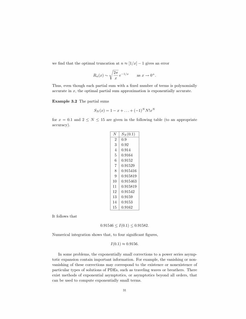
Example 3.2 The partial sums
SN (x) = 1− x+ . . .+ (−1)NN !xN
for x = 0.1 and 2 ≤ N ≤ 15 are given in the following table (to an appropriateaccuracy).
N SN (0.1)2 0.93 0.924 0.9145 0.91646 0.91527 0.915298 0.9154169 0.915819
10 0.91546311 0.91581912 0.9154213 0.915914 0.915315 0.9162
It follows that
0.91546 ≤ I(0.1) ≤ 0.91582.
Numerical integration shows that, to four significant figures,
I(0.1) ≈ 0.9156.
In some problems, the exponentially small corrections to a power series asymp-totic expansion contain important information. For example, the vanishing or non-vanishing of these corrections may correspond to the existence or nonexistence ofparticular types of solutions of PDEs, such as traveling waves or breathers. Thereexist methods of exponential asymptotics, or asymptotics beyond all orders, thatcan be used to compute exponentially small terms.
31

3.2 Perturbed Gaussian integrals
Consider the following integral
I(a, ε) =∫ ∞−∞
exp[−1
2ax2 − εx4
]dx, (3.4)
where a > 0 and ε ≥ 0. For ε = 0, this is a standard Gaussian integral, and
I(a, 0) =1√2πa
.
For ε > 0, we cannot compute I(a, ε) explicitly, but we can obtain an asymptoticexpansion as ε→ 0+.
First, we proceed formally. Taylor expanding the exponential with respect to ε,
exp[−1
2ax2 − εx4
]= e−
12ax
2
1− εx4 +12!ε2x8 + . . .+
(−1)n
n!εnx4n + . . .
,
and integrating the result term-by-term, we get
I(a, ε) ∼ 1√2πa
1− ε〈x4〉+ . . .+
(−1)n
n!εn〈x4n〉+ . . .
, , (3.5)
where
〈x4n〉 =
∫∞−∞ x4ne−
12ax
2dx∫∞
−∞ e−12ax
2dx
.
We use a special case of Wick’s theorem to calculate these integrals.
Proposition 3.3 For m ∈ N, we have
〈x2m〉 =(2m− 1)!!
am,
where
(2m− 1)!! = 1 · 3 · 5 . . . (2m− 3) · (2m− 1).
Proof. Let
J(a, b) =
∫∞−∞ e−
12ax
2+bx dx∫∞−∞ e−
12ax
2dx
.
Differentiating J(a, b) n-times with respect to b and setting b = 0, we find that
〈xn〉 =dn
dbnJ(a, b)
∣∣∣∣b=0
.
Writing
e−12ax
2+bx = e−12a(x−b)
2+ b22a
32

and making the change of variable (x− b) 7→ x in the numerator, we deduce that
J(a, b) = eb22a .
Hence,
〈xn〉 =dn
dbn
[e
b22a
]∣∣∣∣b=0
=dn
dbn
1 +
b2
2a+ . . .+
1m!
b2m
(2a)m+ . . .
∣∣∣∣b=0
,
which implies that
〈x2m〉 =(2m)!
(2a)mm!.
This expression is equivalent to the result.
Using the result of this proposition in (3.5), we conclude that
I(a, ε) ∼ 1√2πa
[1− 3
a2ε+
105a4
ε2 + . . .+ anεn + . . .
]as ε→ 0+, (3.6)
where
an =(−1)n(4n− 1)!!
n!a2n. (3.7)
By the ratio test, the radius of convergence R of this series is
R = limn→∞
(n+ 1)!a2n+2(4n− 1)!n!a2n(4n+ 3)!!
= limn→∞
(n+ 1)a2
(4n+ 1)(4n+ 3)= 0.
Thus, the series diverges for every ε > 0, as could have been anticipated by the factthat I(a, ε) is undefined for ε < 0.
The next proposition shows that the series is an asymptotic expansion of I(a, ε)as ε→ 0+.
Proposition 3.4 Suppose I(a, ε) is defined by (3.4). For each N = 0, 1, 2, . . . andε > 0, we have ∣∣∣∣∣I(a, ε)−
N∑n=0
anεn
∣∣∣∣∣ ≤ CN+1εN+1
where an is given by (3.7), and
CN+1 =1
(N + 1)!
∫ ∞−∞
x4(N+1)e−12ax
2dx.
33

Proof. Taylor’s theorem implies that for y ≥ 0 and N ∈ N
e−y = 1− y +12!y2 + . . .+
(−1)N
N !yN + sN+1(y),
where
sN+1(y) =1
(N + 1)!dN+1
dyN+1
(e−y)∣∣∣∣y=η
yN+1
for some 0 ≤ η ≤ y. Replacing y by εx4 in this equation and estimating theremainder, we find that
e−εx4
= 1− εx4 +12!ε2x4 + . . .+
(−1)N
N !εNx4N + εN+1rN+1(x), (3.8)
where
|rN+1(x)| ≤ x4(N+1)
(N + 1)!.
Using (3.8) in (3.4), we get
I(a, ε) =N∑n=0
anεn + εN+1
∫ ∞−∞
rN+1(x)e−12ax
2dx.
It follows that∣∣∣∣∣I(a, ε)−N∑n=0
anεn
∣∣∣∣∣ ≤ εN+1
∫ ∞−∞|rN+1(x)| e− 1
2ax2dx
≤ εN+1 1(N + 1)!
∫ ∞−∞
x4(N+1)e−12ax
2dx,
which proves the result.
These expansions generalize to multi-dimensional Gaussian integrals, of the form
I(A, ε) =∫
Rn
exp(−1
2xTAx+ εV (x)
)dx
where A is a symmetric n×nmatrix, and to infinite-dimensional functional integrals,such as those given by the formal expression
I(ε) =∫
exp−∫ (
12|∇u(x)|2 +
12u2(x) + εV (u(x))
)dx
Du
which appear in quantum field theory and statistical physics.
34

3.3 The method of stationary phase
The method of stationary phase provides an asymptotic expansion of integrals witha rapidly oscillating integrand. Because of cancelation, the behavior of such integralsis dominated by contributions from neighborhoods of the stationary phase pointswhere the oscillations are the slowest.
Example 3.5 Consider the following Fresnel integral
I(ε) =∫ ∞−∞
eit2/ε dt.
This oscillatory integral is not defined as an absolutely convergent integral, since∣∣∣eit2/ε∣∣∣ = 1, but it can be defined as an improper integral,
I(ε) = limR→∞
∫ R
−Reit
2/ε dt.
This convergence follows from an integration by parts:∫ R
1
eit2/ε dt =
[ ε2it
eit2/ε]R1
+∫ R
1
ε
2it2eit
2/ε dt.
The integrand oscillates rapidly away from the stationary phase point t = 0, andthese parts contribute terms that are smaller than any power of ε, as we show below.The first oscillation near t = 0, where cancelation does not occur, has width of theorder ε1/2, so we expect that I(ε) = O(ε1/2) as ε→ 0.
In fact, using contour integration and changing variables t 7→ eiπ/4s if ε > 0 andt 7→ E−iπ/4s if ε < 0, one can show that∫ ∞
−∞eit
2/ε dt =eiπ/4
√2π|ε| if ε > 0
e−iπ/4√
2π|ε| if ε < 0.
Next, we consider the integral
I(ε) =∫ ∞−∞
f(t)eiϕ(t)/ε dt, (3.9)
where f : R→ C and ϕ : R→ R are smooth functions. A point t = c is a stationaryphase point if ϕ′(c) = 0. We call the stationary phase point nondegenerate ifϕ′′(c) 6= 0.
Suppose that I has a single stationary phase point at t = c, which is nondegen-erate. (If there are several such points, we simply add together the contributionsfrom each one.) Then, using the idea that only the part of the integrand near thestationary phase point t = c contributes significantly, we can Taylor expand thefunction f and the phase ϕ to approximate I(ε) as follows:
I(ε) ∼∫f(c) exp
i
ε
[ϕ(c) +
12ϕ′′(c)(t− c)2
]dt
35

∼ f(c)eiϕ(c)/ε
∫exp
[iϕ′′(c)
2εs2]ds
∼
√2πε|ϕ′′(c)|
f(c)eiϕ(c)/ε+iσπ/4,
where
σ = sgnϕ′′(c).
More generally, we consider the asymptotic behavior as ε → 0 of an integral ofthe form
I(x, ε) =∫A(x, ξ)eiϕ(x,ξ)/ε dξ, (3.10)
where x ∈ Rn and ξ ∈ Rm. We assume that
ϕ : Rn × Rm → R, A : Rn × Rm → C
are smooth (C∞) functions, and that the support of A,
suppA = (x, ξ) ∈ Rn × Rm | A(x, ξ) 6= 0,
is a compact subset of Rn × Rm.
Definition 3.6 A stationary, or critical, point of the phase ϕ is a point (x, ξ) ∈Rn × Rm such that
∂ϕ
∂ξ(x, ξ) = 0. (3.11)
A stationary phase point is nondegenerate if
∂2ϕ
∂ξ2=(
∂2ϕ
∂ξi∂ξj
)i,j=1,...,m
is invertible at the stationary phase point.
Proposition 3.7 If the support of A contains no stationary points of ϕ, then
I(x, ε) = O (εn) as ε→ 0
for every n ∈ N.
Proof. Rewriting the integral in (3.10), and integrating by parts, we have
I(x, ε) = −iε∫A∂ϕ
∂ξ· ∂∂ξ
[eiϕ/ε
] ∣∣∣∣∂ϕ∂ξ∣∣∣∣−2
dξ
= iε
∫∂
∂ξ·
[A
∣∣∣∣∂ϕ∂ξ∣∣∣∣−2
∂ϕ
∂ξ
]eiϕ/ε dξ
= O(ε).
36

Applying this argument n times, we get the result.
The implicit function theorem implies there is a unique local smooth solution of(3.11) for ξ in a neighborhood U × V ⊂ Rn × Rm We write this stationary phasepoint as as ξ = ξ(x), where ξ : U → V . We may reduce the case of multiplenondegenerate critical points to this one by means of a partition of unity, and mayalso suppose that suppA ⊂ U × V. According to the Morse lemma, there is a localchange of coordinates ξ 7→ η near a nondegenerate critical point such that
ϕ(x, ξ) = ϕ(x, ξ(x)
)+
12∂2ϕ
∂ξ2(x, ξ(x)
)· (η, η).
Making this change of variables in (3.10), and evaluating the resulting Fresnel inte-gral, we get the following stationary phase formula [10].
Theorem 3.8 Let I(x, ε) be defined by (3.10), where ϕ is a smooth real-valuedfunction with a nondegenerate stationary phase point at (x, ξ(x)), and A is a com-pactly supported smooth function whose support is contained in a sufficiently smallneighborhood of the stationary phase point. Then, as ε→ 0,
I(x, ε) ∼ (2πε)n/2√det∣∣∣∂2ϕ∂ξ2
∣∣∣ξ=ξ(x)
eiϕ(x,ξ(x))/ε+iπσ/4∞∑p=0
(iε)pRp(x),
where
σ = sgn(∂2ϕ
∂ξ2
)ξ=ξ(x)
is the signature of the matrix (the difference between the number of positive andnegative eigenvalues), R0 = 1, and
Rp(x) =∑|k|≤2p
Rpk(x)∂kA
∂ξk
∣∣∣∣ξ=ξ(x)
,
where the Rpk are smooth functions depending only on ϕ.
3.4 Airy functions and degenerate stationary phase points
The behavior of the integral in (3.10) is more complicated when it has degeneratestationary phase points. Here, we consider the simplest case, where ξ ∈ R andtwo stationary phase points coalesce. The asymptotic behavior of the integral in aneighborhood of the degenerate critical point is then described by an Airy function.
Airy functions are solutions of the ODE
y′′ = xy. (3.12)
37

The behavior of these functions is oscillatory as x → −∞ and exponential as x →∞. They are the most basic functions that exhibit a transition from oscillatoryto exponential behavior, and because of this they arise in many applications (forexample, in describing waves at caustics or turning points).
Two linearly independent solutions of (3.12) are denoted by Ai(x) and Bi(x).The solution Ai(x) is determined up to a constant normalizing factor by the condi-tion that Ai(x)→ 0 as x→∞. It is conventionally normalized so that
Ai(0) =1
32/3Γ(
23
),
where Γ is the Gamma-function. This solution decays exponentially as x→∞ andoscillates, with algebraic decay, as x→ −∞ [16],
Ai(x) ∼
12π−1/2x−1/4 exp[−2x3/2/3] as x→∞,
π−1/2(−x)−1/4 sin[2(−x)3/2/3 + π/4] as x→ −∞.
The solution Bi(x) grows exponentially as x→∞.We can derive these results from an integral representation of Ai(x) that is
obtained by taking the Fourier transform of (3.12).∗ Let y = F [y] denote theFourier transform of y,
y(k) =1
2π
∫ ∞−∞
y(x)e−ikx dx,
y(x) =∫ ∞−∞
y(k)eikx dk.
Then
F [y′′] = −k2y, F [−ixy] = y′.
Fourier transforming (3.12), we find that
−k2y = iy′.
Solving this first-order ODE, we get
y(k) = ceik3/3,
so y is given by the oscillatory integral
y(x) = c
∫ ∞−∞
ei(kx+k3/3) dk.
∗We do not obtain Bi by this method because it grows exponentially as x→∞, which is too fast
for its Fourier transform to be well-defined, even as a tempered distribution.
38

The standard normalization for the Airy function corresponds to c = 1/(2π), andthus
Ai(x) =1
2π
∫ ∞−∞
ei(kx+k3/3) dk. (3.13)
This oscillatory integral is not absolutely convergent, but it can be interpretedas the inverse Fourier transform of a tempered distribution. The inverse transformis a C∞ function that extends to an entire function of a complex variable, as canbe seen by shifting the contour of integration upwards to obtain the absolutelyconvergent integral representation
Ai(x) =1
2π
∫ ∞+iη
−∞+iη
ei(kx+k3/3) dk.
Just as the Fresnel integral with a quadratic phase, provides an approximationnear a nondegenerate stationary phase point, the Airy integral with a cubic phaseprovides an approximation near a degenerate stationary phase point in which thethird derivative of the phase in nonzero. This occurs when two nondegeneratestationary phase points coalesce.
Let us consider the integral
I(x, ε) =∫ ∞−∞
f(x, t)eiϕ(x,t)/ε dt.
Suppose that we have nondegenerate stationary phase points at
t = t±(x)
for x < x0, which are equal when x = x0 so that t±(x0) = t0. We assume that
ϕt (x0, t0) = 0, ϕtt (x0, t0) = 0, ϕttt (x0, t0) 6= 0.
Then Chester, Friedman, and Ursell (1957) showed that in a neighborhood of (x0, t0)there is a local change of variables t = τ(x, s) and functions ψ(x), ρ(x) such that
ϕ(x, t) = ψ(x) + ρ(x)s+13s3.
Here, we have τ(x0, 0) = t0 and ρ(x0) = 0. The stationary phase points correspondto s = ±
√−ρ(x), where ρ(x) < 0 for x < x0.
Since the asymptotic behavior of the integral as ε → 0 is dominated by thecontribution from the neighborhood of the stationary phase point, we expect that
I(x, ε) ∼∫ ∞−∞
f (x, τ(x, s)) τs(x, s)ei[ψ(x)+ρ(x)s+ 13 s
3]/ε ds
∼ f (x0, t0) τs(x0, 0)eiψ(x)/ε
∫ ∞−∞
ei[ρ(x)s+13 s
3]/ε ds
39

∼ ε1/3f (x0, t0) τs(x0, 0)eiψ(x)/ε
∫ ∞−∞
ei[ε−2/3ρ(x)k+ 1
3k3] dk
∼ 2πε1/3f (x0, t0) τs(x0, 0)eiψ(x)/εAi(ρ(x)ε2/3
),
where we have made the change of variables s = ε1/3k, and used the definition ofthe Airy function.
More generally, we have the following result. For the proof, see [10].
Theorem 3.9 Let I(x, ε) be defined by (3.10), where ϕ(x, ξ), with x ∈ Rd andξ ∈ R, is a smooth, real-valued function with a degenerate stationary phase pointat (x, ξ(x)). Suppose that
∂ϕ
∂ξ= 0,
∂2ϕ
∂ξ2= 0,
∂3ϕ
∂ξ36= 0,
at ξ = ξ(x), and A(x, ξ) is a smooth function whose support is contained in asufficiently small neighborhood of the degenerate stationary phase point. Thenthere are smooth real-valued functions ψ(x), ρ(x), and smooth functions Ak(x),Bk(x) such that
I(x, ε) ∼
[ε1/3Ai
(ρ(x)ε2/3
) ∞∑k=0
Ak(x) + iε2/3Ai′(ρ(x)ε2/3
) ∞∑k=0
Bk(x)
]eiψ(x)/ε
as ε→ 0.
3.4.1 Dispersive wave propagation
An important application of the method of stationary phase concerns the long-time, or large-distance, behavior of linear dispersive waves. Kelvin (1887) originallydeveloped the method for this purpose, following earlier work by Cauchy, Stokes,and Riemann. He used it to study the pattern of dispersive water waves generatedby a ship in steady motion, and showed that at large distances from the ship thewaves form a wedge with a half-angle of sin−1(1/3), or approximately 19.5.
As a basic example of a dispersive wave equation, we consider the followingIVP (initial value problem) for the linearized KdV (Korteweg-de Vries), or Airy,equation,
ut = uxxx,
u(x, 0) = f(x).
This equation provides an asymptotic description of linear, unidirectional, weaklydispersive long waves; for example, shallow water waves.
40

We assume for simplicity that the initial data f : R→ R is a Schwarz function,meaning that it is smooth and decays, together with all its derivatives, faster thanany polynomial as |x| → ∞.
We use u(k, t) to denote the Fourier transform of u(x, t) with respect to x,
u(x, t) =∫ ∞−∞
u(k, t)eikx dk,
u(k, t) =1
2π
∫ ∞−∞
u(x, t)e−ikx dx.
Then u(k, t) satisfies
ut + ik3u = 0,
u(k, 0) = f(k).
The solution of this equation is
u(k, t) = f(k)e−iω(k)t,
where
ω(k) = k3.
The function ω : R→ R gives the (angular) frequency ω(k) of a wave with wavenum-ber k, and is called the dispersion relation of the KdV equation.
Inverting the Fourier transform, we find that the solution is given by
u(x, t) =∫ ∞−∞
f(k)eikx−iω(k)t dk.
Using the convolution theorem, we can write this solution as
u(x, t) = f ∗ g(x, t),
where the star denotes convolution with respect to x, and
g(x, t) =1
(3t)1/3Ai(− x
(3t)1/3
)is the Green’s function of the Airy equation.
We consider the asymptotic behavior of this solution as t → ∞ with x/t = v
fixed. This limit corresponds to the large-time limit in a reference frame movingwith velocity v. Thus, we want to find the behavior as t→∞ of
u(vt, t) =∫ ∞−∞
f(k)eiϕ(k,v)t dk, (3.14)
where
ϕ(k, v) = kv − ω(k).
41

The stationary phase points satisfy ϕk = 0, or
v = ω′(k).
The solutions are the wavenumbers k whose group velocity ω′(k) is equal to v. Itfollows that
3k2 = v.
If v < 0, then there are no stationary phase points, and u(vt, t) = o(t−n) ast→∞ for any n ∈ N.
If v > 0, then there are two nondegenerate stationary phase points at k =±k0(v), where
k0(v) =√v
3.
These two points contribute complex conjugate terms, and the method of stationaryphase implies that
u(vt, t) ∼
√2π
|ω′′(k0)|tf(k0)eiϕ(k0,v)t−iπ/4 + c.c. as t→∞.
The energy in the wave-packet therefore propagates at the group velocity C = ω′(k),
C = 3k2,
rather than the phase velocity c = ω/k,
c = k2.
The solution decays at a rate of t−1/2, in accordance with the linear growth in t ofthe length of the wavetrain and the conservation of energy,∫ ∞
−∞u2(x, t) dt = constant.
The two stationary phase points coalesce when v = 0, and then there is a singledegenerate stationary phase point. To find the asymptotic behavior of the solutionwhen v is small, we make the change of variables
k =ξ
(3t)1/3
in the Fourier integral solution (3.14), which gives
u(x, t) =1
(3t)1/3
∫ ∞−∞
f
(ξ
(3t)1/3
)e−i(ξw+ 1
3 ξ3) dξ,
42

where
w = − t2/3v
31/3.
It follows that as t→∞ with t2/3v fixed,
u(x, t) ∼ 2π(3t)1/3
f(0)Ai(− t
2/3v
31/3
).
Thus the transition between oscillatory and exponential behavior is described byan Airy function. Since v = x/t, the width of the transition layer is of the ordert1/3 in x, and the solution in this region is of the order t−1/3. Thus it decays moreslowly and is larger than the solution elsewhere.
Whitham [20] gives a detailed discussion of linear and nonlinear dispersive wavepropagation.
3.5 Laplace’s Method
Consider an integral
I(ε) =∫ ∞−∞
f(t)eϕ(t)/ε dt,
where ϕ : R → R and f : R → C are smooth functions, and ε is a small positiveparameter. This integral differs from the stationary phase integral in (3.9) becausethe argument of the exponential is real, not imaginary. Suppose that ϕ has a globalmaximum at t = c, and the maximum is nondegenerate, meaning that ϕ′′(c) < 0.The dominant contribution to the integral comes from the neighborhood of t = c,since the integrand is exponentially smaller in ε away from that point. Taylorexpanding the functions in the integrand about t = c, we expect that
I(ε) ∼∫f(c)e[ϕ(c)+ 1
2ϕ′′(c)(t−c)2]/ε dt
∼ f(c)eϕ(c)/ε
∫ ∞−∞
e12ϕ′′(c)(t−c)2/ε dt.
Using the standard integral ∫ ∞−∞
e−12at
2dt =
√2πa,
we get
I(ε) ∼ f(c)(
2πε|ϕ′′(c)|
)1/2
eϕ(c)/ε as ε→ 0+.
This result can proved under suitable assumptions on f and ϕ, but we will not givea detailed proof here (see [17], for example).
43

Example 3.10 The Gamma function Γ : (0,∞)→ R is defined by
Γ(x) =∫ ∞
0
e−ttx−1 dt.
Integration by parts shows that if n ∈ N, then
Γ(n+ 1) = n!.
Thus, the Gamma function extends the factorial function to arbitrary positive realnumbers. In fact, the Gamma function can be continued to an analytic function
Γ : C \ 0,−1,−2, . . . → C
with simple poles at 0,−1,−2, . . ..Making the change of variables t = xs, we can write the integral representation
of Γ as
Γ(x) = xx∫ ∞
0
1sexϕ(s) ds,
where
ϕ(s) = −s+ log s.
The phase ϕ(s) has a nondegenerate maximum at s = 1, where ϕ(1) = −1, andϕ′′(1) = −1. Using Laplace’s method, we find that
Γ(x) ∼(
2πx
)1/2
xxe−x as x→∞.
In particular, setting x = n+ 1, and using the fact that
limn→∞
(n+ 1n
)n= e,
we obtain Stirling’s formula for the factorial,
n! ∼ (2π)1/2nn+1/2e−n as n→∞.
This expansion of the Γ-function can be continued to higher orders to give:
Γ(x) ∼(
2πx
)1/2
xxe−x[1 +
a1
x+a2
x2+a3
x3+ . . .
]as x→∞,
a1 =112, a2 =
1288
, a3 = − 13951, 840
, . . . .
44
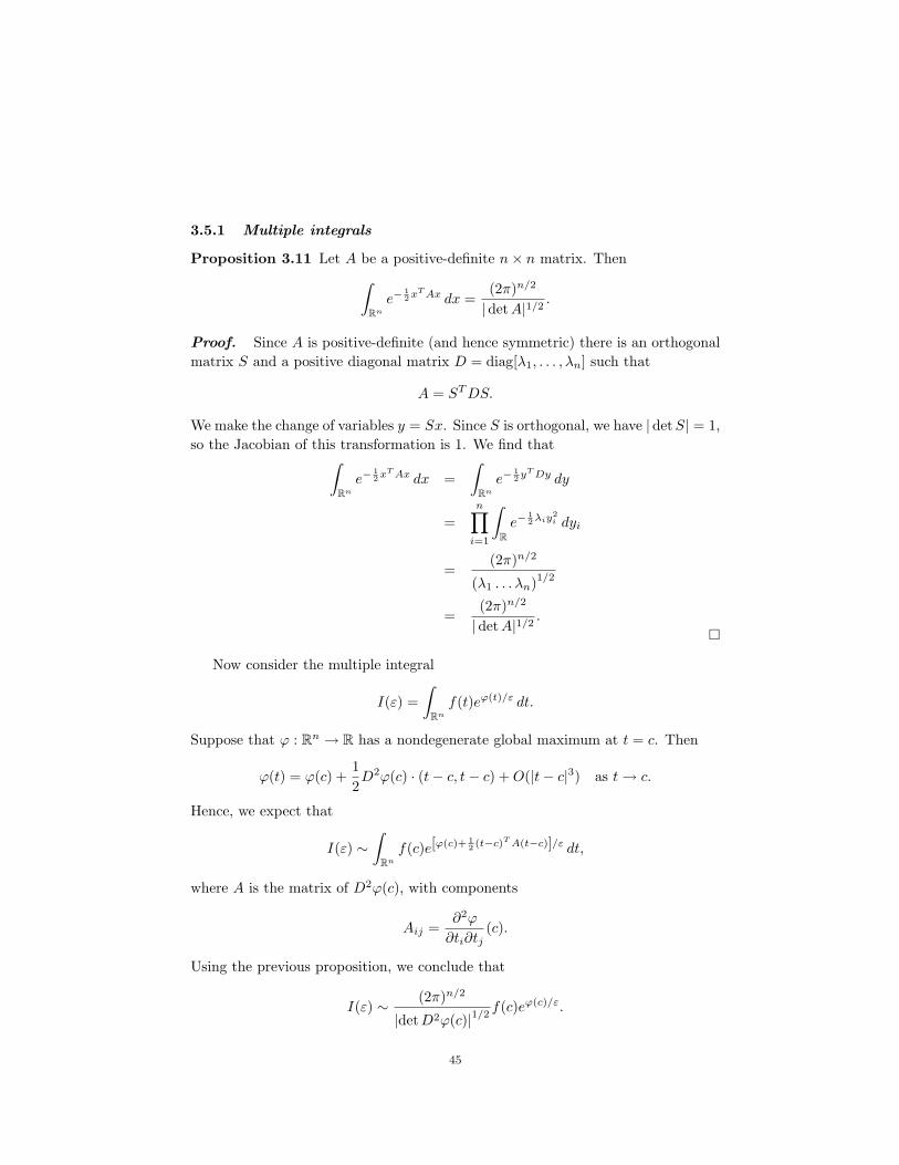
3.5.1 Multiple integrals
Proposition 3.11 Let A be a positive-definite n× n matrix. Then∫Rn
e−12x
TAx dx =(2π)n/2
|detA|1/2.
Proof. Since A is positive-definite (and hence symmetric) there is an orthogonalmatrix S and a positive diagonal matrix D = diag[λ1, . . . , λn] such that
A = STDS.
We make the change of variables y = Sx. Since S is orthogonal, we have |detS| = 1,so the Jacobian of this transformation is 1. We find that∫
Rn
e−12x
TAx dx =∫
Rn
e−12y
TDy dy
=n∏i=1
∫Re−
12λiy
2i dyi
=(2π)n/2
(λ1 . . . λn)1/2
=(2π)n/2
|detA|1/2.
Now consider the multiple integral
I(ε) =∫
Rn
f(t)eϕ(t)/ε dt.
Suppose that ϕ : Rn → R has a nondegenerate global maximum at t = c. Then
ϕ(t) = ϕ(c) +12D2ϕ(c) · (t− c, t− c) +O(|t− c|3) as t→ c.
Hence, we expect that
I(ε) ∼∫
Rn
f(c)e[ϕ(c)+ 12 (t−c)TA(t−c)]/ε dt,
where A is the matrix of D2ϕ(c), with components
Aij =∂2ϕ
∂ti∂tj(c).
Using the previous proposition, we conclude that
I(ε) ∼ (2π)n/2
|detD2ϕ(c)|1/2f(c)eϕ(c)/ε.
45

3.6 The method of steepest descents
Consider a contour integral of the form
I(λ) =∫C
f(z)eλh(z) dz,
where C is a contour in the complex plane, and f, h : C→ C are analytic functions.If h(x+ iy) = ϕ(x, y) + iψ(x, y) is analytic, then ϕ,ψ : R2 → R have no maxima
or minima, and critical points where h′(z) = 0 are saddle points of ϕ, ψ. The curvesϕ = constant, ψ = constant are orthogonal except at critical points.
The idea of the method of steepest descents is to deform the contour C into asteepest descent contour passing through a saddle point on which ϕ has a maximumand ψ = constant, so the contour is orthogonal to the level curves of ϕ. We thenapply Laplace’s method to the resulting integral. We will illustrate this idea byderiving the asymptotic behavior of the Airy function, given by (3.13)
Ai(x) =1
2π
∫ ∞−∞
ei(kx+k3/3) dk.
To obtain the asymptotic behavior of Ai(x) as x → ∞, we put this integralrepresentation in a form that is suitable for the method of steepest descents. Settingk = x1/2z, we find that
Ai(x) =1
2πx1/2I
(x3/2
),
where
I(λ) =∫ ∞−∞
eiλ[z+13 z
3] dz.
The phase
h(z) = i
(z +
13z3
)has critical points at z = ±i.
Writing h = ϕ+ iψ in terms of its real and imaginary parts, we have
ϕ(x, y) = −y(
1 + x2 − 13y2
),
ψ(x, y) = x
(1 +
13x2 − y2
).
The steepest descent contour ψ(x, y) = 0 through z = i, or (x, y) = (0, 1), is
y =
√1 +
13x2.
46

When λ > 0, we can deform the integration contour (−∞,∞) upwards to thissteepest descent contour C, since the integrand decays exponentially as |z| → ∞ inthe upper-half plane. Thus,
I(λ) =∫C
eiλ[z+13 z
3] dz.
We parameterize C by z(t) = x(t) + iy(t), where
x(t) =√
3 sinh t, y(t) = cosh t.
Then we find that
I(λ) =∫ ∞−∞
f(t)eiλϕ(t) dt,
where
f(t) =√
3 cosh t+ i sinh t,
ϕ(t) = cosh t[2− 8
3cosh2 t
].
The maximum of ϕ(t) occurs at t = 0, where
ϕ(0) = −2/3, ϕ′(0) = 0, ϕ′′(0) = −6.
Laplace’s method implies that
I(λ) ∼ f(0)(
2π−λϕ′′(0)
)1/2
eλϕ(0)
∼(πλ
)1/2
e−2λ/3.
It follows that
Ai(x) ∼ 12π1/2x1/4
e−2x3/2/3 as x→∞. (3.15)
Using the method of stationary phase, one can show from (3.13) that the asymp-totic behavior of the Airy function as x→ −∞ is given by
Ai(x) ∼ 1π1/2|x|1/4
sin[
23|x|3/2 +
π
4
]. (3.16)
This result is an example of a connection formula. It gives the asymptotic behavioras x→ −∞ of the solution of the ODE (3.12) that decays exponentially as x→∞.This connection formula is derived using the integral representation (3.13), whichprovides global information about the solution.
47

48

Chapter 4
The Method of Matched AsymptoticExpansions: ODEs
Many singularly perturbed differential equations have solutions that change rapidlyin a narrow region. This may occur in an initial layer where there is a rapidadjustment of initial conditions to a quasi-steady state, in a boundary layer wherethe solution away from the boundary adjusts to a boundary condition, or in aninterior layer such as a propagating wave-front.
These problems can be analyzed using the method of matched asymptotic ex-pansions (MMAE), in which we construct different asymptotic solutions inside andoutside the region of rapid change, and ‘match’ them together to determine a globalsolution. A typical feature of this type of problem is a reduction in the order ofthe differential equation in the unperturbed problem, leading to a reduction in thenumber of initial or boundary conditions that can be imposed upon the solution.For additional information, see [3], [19].
4.1 Enzyme kinetics
Enzymes are proteins that act as catalysts. (There are also a smaller number ofenzymes, called ribozymes, that contain catalytic RNA molecules.) A substancethat is acted upon by an enzyme to create a product is called a substrate. Enzymesare typically very specific and highly efficient catalysts — tiny concentrations ofenzymes compared with substrate concentrations are required.
For example, the enzyme catalase catalyzes the decomposition of hydrogen per-oxide into water and oxygen, and one molecule of catalase can break up 40 millionmolecules of hydrogen peroxide each second. As another example, carbonic anhy-drase occurs in red blood cells, where it catalyzes the reaction CO2+H2O↔ H2CO3
that enables the cells to transport carbon dioxide from the tissues to the lungs. Onemolecule of carbonic anhydrase can process one million molecules of CO2 each sec-ond.
Michaelis and Menton (1913) proposed a simple model of enzymatically con-trolled reactions, in which the enzyme E and substrate S combine to form a com-
49

plex C, and the complex breaks down irreversibly into the enzyme and a productP . Symbolically, we have
E + S ←→ C −→ E + P.
We let
e = [E], s = [S], c = [C], p = [P ],
denote the concentrations of the corresponding species.According to the law of mass action, the rate of a reaction is proportional to the
product of the concentrations of the species involved, so that
de
dt= −k0es+ (k0 + k2) c,
ds
dt= −k1es+ k0c,
dc
dt= k1es− (k0 + k2) c,
dp
dt= k2c,
where k0, k1, k2 are rate constants. We impose initial conditions
s(0) = s0, e(0) = e0, c(0) = c0, p(0) = 0,
corresponding to an initial state with substrate and enzyme but no complex orproduct.
The equation for p decouples from the remaining equations. Adding the equa-tions for e and c, we get
d
dt(e+ c) = 0,
which implies that
e(t) + c(t) = e0.
Thus, the equations reduce to a pair of ODEs for s and c:
ds
dt= −k1e0s+ (k1s+ k0) c,
dc
dt= k1e0s− (k1s+ k0 + k2) c,
s(0) = s0, c(0) = 0.
We introduce dimensionless quantities
u(τ) =s(t)s0
, v(τ) =c(t)e0
, τ = k1e0t,
50
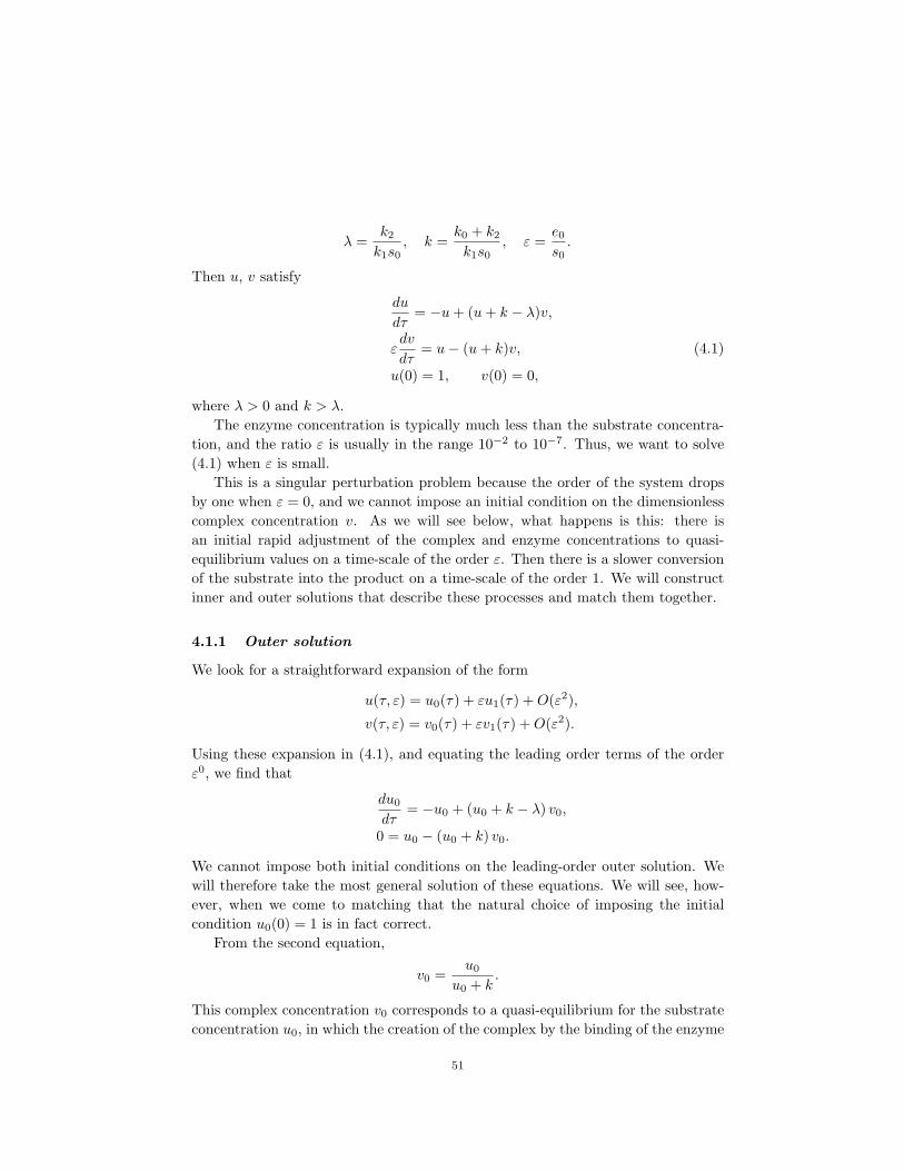
λ =k2
k1s0, k =
k0 + k2
k1s0, ε =
e0s0.
Then u, v satisfy
du
dτ= −u+ (u+ k − λ)v,
εdv
dτ= u− (u+ k)v, (4.1)
u(0) = 1, v(0) = 0,
where λ > 0 and k > λ.The enzyme concentration is typically much less than the substrate concentra-
tion, and the ratio ε is usually in the range 10−2 to 10−7. Thus, we want to solve(4.1) when ε is small.
This is a singular perturbation problem because the order of the system dropsby one when ε = 0, and we cannot impose an initial condition on the dimensionlesscomplex concentration v. As we will see below, what happens is this: there isan initial rapid adjustment of the complex and enzyme concentrations to quasi-equilibrium values on a time-scale of the order ε. Then there is a slower conversionof the substrate into the product on a time-scale of the order 1. We will constructinner and outer solutions that describe these processes and match them together.
4.1.1 Outer solution
We look for a straightforward expansion of the form
u(τ, ε) = u0(τ) + εu1(τ) +O(ε2),
v(τ, ε) = v0(τ) + εv1(τ) +O(ε2).
Using these expansion in (4.1), and equating the leading order terms of the orderε0, we find that
du0
dτ= −u0 + (u0 + k − λ) v0,
0 = u0 − (u0 + k) v0.
We cannot impose both initial conditions on the leading-order outer solution. Wewill therefore take the most general solution of these equations. We will see, how-ever, when we come to matching that the natural choice of imposing the initialcondition u0(0) = 1 is in fact correct.
From the second equation,
v0 =u0
u0 + k.
This complex concentration v0 corresponds to a quasi-equilibrium for the substrateconcentration u0, in which the creation of the complex by the binding of the enzyme
51
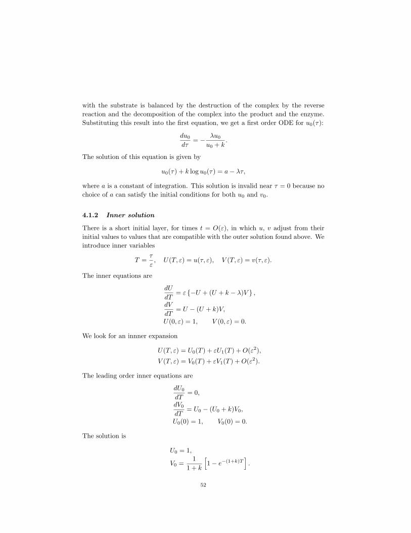
with the substrate is balanced by the destruction of the complex by the reversereaction and the decomposition of the complex into the product and the enzyme.Substituting this result into the first equation, we get a first order ODE for u0(τ):
du0
dτ= − λu0
u0 + k.
The solution of this equation is given by
u0(τ) + k log u0(τ) = a− λτ,
where a is a constant of integration. This solution is invalid near τ = 0 because nochoice of a can satisfy the initial conditions for both u0 and v0.
4.1.2 Inner solution
There is a short initial layer, for times t = O(ε), in which u, v adjust from theirinitial values to values that are compatible with the outer solution found above. Weintroduce inner variables
T =τ
ε, U(T, ε) = u(τ, ε), V (T, ε) = v(τ, ε).
The inner equations are
dU
dT= ε −U + (U + k − λ)V ,
dV
dT= U − (U + k)V,
U(0, ε) = 1, V (0, ε) = 0.
We look for an innner expansion
U(T, ε) = U0(T ) + εU1(T ) +O(ε2),
V (T, ε) = V0(T ) + εV1(T ) +O(ε2).
The leading order inner equations are
dU0
dT= 0,
dV0
dT= U0 − (U0 + k)V0,
U0(0) = 1, V0(0) = 0.
The solution is
U0 = 1,
V0 =1
1 + k
[1− e−(1+k)T
].
52

4.1.3 Matching
We assume that the inner and outer expansions are both valid for intermediatetimes of the order ε τ 1. We require that the expansions agree asymptoticallyin this regime, where T →∞ and τ → 0 as ε→ 0. Hence, the matching conditionis
limT→∞
U0(T ) = limτ→0+
u0(τ),
limT→∞
V0(T ) = limτ→0+
v0(τ).
This condition implies that
u0(0) = 1, v0(0) =1
1 + k,
which is satisfied when a = 1 in the outer solution. Hence
u0(τ) + k log u0(τ) = 1− λτ.
The slow manifold for the enzyme system is the curve
v =u
u+ k.
Trajectories rapidly approach the slow manifold in the initial layer. They then movemore slowly along the slow manifold and approach the equilibrium u = v = 0 asτ → ∞. The inner layer corresponds to the small amount of enzyme ‘loading up”on the substrate. The slow manifold corresponds to the enzyme working at fullcapacity in converting substrate into product.
A principle quantity of biological interest is the rate of uptake,
r0 =du0
dτ
∣∣∣∣τ=0
.
It follows from the outer solution that
r0 =λ
1 + k.
The dimensional form of the rate of uptake is
R0 =ds
dt
=Qs0
s0 + km
where Q = k2e0 is the maximum reaction rate, and
km =k0 + k2
k1
is the Michaelis constant. The maximum rate depends only on k2; the rate limitingstep is C → P + E.
53

For more information about enzyme kinetics, see [12].
4.2 General initial layer problems
Consider a dynamical system for x(t) ∈ Rm, y(t) ∈ Rn:
x = f(x, y),
εy = g(x, y), (4.2)
x(0) = x0, y(0) = y0.
Here, f : Rm × Rn → Rm, g : Rm × Rn → Rn. Suppose that there is a functionϕ : Rm → Rn such that
g (x, ϕ(x)) = 0,
and for each fixed x ∈ Rn, the solution y = ϕ(x) is a globally asymptotically stableequilibrium of the ‘fast’ system
εy(t) = g (x, y(t)) . (4.3)
Then the behavior of solutions of (4.2) is as follows:
(a) for t = O(ε), there is a short initial layer in which x(t) is nearly constant,and close to its initial value x0, and y(t) changes rapidly from its initialvalue to the quasi-steady state y = ϕ(x0).
(b) for t = O(1), the solution is close to the slow manifold y = ϕ(x) + O(ε),and x(t) satisfies
x = f (x, ϕ(x)) .
If (4.3) does not have a unique globally stable equilibrium for every x ∈ Rm,then more complex phenomena can occur.
An interesting example of a fast-slow system of ODEs arises in modeling thephenomenon of bursting in pancreatic β-cells. These cells are responsible for pro-ducing insulin which regulates glucose levels in the body. The β-cells are observedto undergo ‘bursting’ in which their membrane potential oscillates rapidly, withperiods of the order of milliseconds. These oscillations stimulate the secretion ofinsulin by the cell. The length of each bursting period is on the order of seconds,and its length is influenced by the amount of glucose in the bloodstream. Thus,this mechanism provides one way that the body regulates glucose.
The basic mathematical model of bursting [12] consists of a fast/slow system.The fast system undergoes a Hopf bifurcation, corresponding to the appearance ofa limit cycle oscillation, as the slow variable increases. On further increase in theslow variable the limit cycle disappears at a homoclinic bifurcation, and the fastsystem switches to a stable quasi-steady states. A decrease in the slow variable
54

leads to a saddle-node bifurcation which destroys this quasi-steady state. Whenthe fast system is in its limit-cycle state, it drives an increase in the slow variable,and when the fast system is in its quasi-steady state it drives a decrease in the slowvariable. The overall effect of this dynamics is a periodic oscillation of the slowvariable on a long time scale which switches on and off the rapid periodic burstingof the fast system.
4.3 Boundary layer problems
The following explicitly solvable model boundary-value problem for a second orderlinear ODE illustrates the phenomenon of boundary layers:
εy′′ + 2y′ + y = 0, 0 < x < 1, (4.4)
y(0) = 0, y(1) = 1.
Here, the prime denotes a derivative with respect to x, and ε is a small positiveparameter. The order of the ODE reduces from two to one when ε = 0, so wecannot expect to impose both boundary conditions on the solution. As we will see,when ε is small, there is a thin boundary layer (of width the order of ε) near x = 0where the solution changes rapidly to take on the boundary value.
4.3.1 Exact solution
The exponential solutions of this equation are y = emx where
m =−1±
√1− ε
ε.
We write these roots as m = −α,−β/ε where
α(ε) =1−√
1− εε
=12
+O(ε),
β(ε) = 1 +√
1− ε= 2 +O(ε).
The general solution is
y(x, ε) = ae−α(ε)x + be−β(ε)x/ε.
Imposing the boundary conditions and solving for the constants of integration a, b,we find that
y(x, ε) =e−αx − e−βx/ε
e−α − e−β/ε.
55

Thus, the solution involves two terms which vary on widely different length-scales.Let us consider the behavior of this solution as ε→ 0+. The asymptotic behavior
is nonuniform, and there are two cases, which lead to matching outer and innersolutions.
(a) Outer limit : x > 0 fixed and ε→ 0+. Then
y(x, ε)→ y0(x),
where
y0(x) =e−x/2
e−1/2. (4.5)
This leading-order outer solution satisfies the boundary condition at x = 1but not the boundary condition at x = 0. Instead, y0(0) = e1/2.
(b) Inner limit : x/ε = X fixed and ε→ 0+. Then
y(εX, ε)→ Y0(X),
where
Y0(X) =1− e−2X
e−1/2.
This leading-order inner solution satisfies the boundary condition at x = 0,but not the one at x = 1, which corresponds to X = 1/ε. Instead, we havelimX→∞ Y0(X) = e1/2.
(c) Matching : Both the inner and outer expansions are valid in the regionε x 1, corresponding to x → 0 and X → ∞ as ε → 0. They satisfythe matching condition
limx→0+
y0(x) = limX→∞
Y0(X).
Let us construct an asymptotic solution of (4.4) without relying on the fact thatwe can solve it exactly.
4.3.2 Outer expansion
We begin with the outer solution. We look for a straightforward expansion
y(x, ε) = y0(x) + εy1(x) +O(ε2).
We use this expansion in (4.4) and equate the coefficients of the leading-order termsto zero. Guided by our analysis of the exact solution, we only impose the boundarycondition at x = 1. We will see later that matching is impossible if, instead, we
56

attempt to impose the boundary condition at x = 0. We obtain that
2y′0 + y0 = 0,
y0(1) = 1.
The solution is given by (4.5), in agreement with the expansion of the exact solution.
4.3.3 Inner expansion
Next, we consider the inner solution. We suppose that there is a boundary layer atx = 0 of width δ(ε), and introduce a stretched inner variable X = x/δ. We look foran inner solution
Y (X, ε) = y(x, ε).
Sinced
dx=
1δ
d
dX,
we find from (4.4) that Y satisfies
ε
δ2Y ′′ +
2δY ′ + Y = 0,
where the prime denotes a derivative with respect to X. There are two possibledominant balances in this equation: (a) δ = 1, leading to the outer solution; (b)δ = ε, leading to the inner solution. Thus, we conclude that the boundary layerthickness is of the order ε, and the appropriate inner variable is
X =x
ε.
The equation for Y is then
Y ′′ + 2Y ′ + εY = 0,
Y (0, ε) = 0.
We impose only the boundary condition at X = 0, since we do not expect the innerexpansion to be valid outside the boundary layer where x = O(ε).
We seek an inner expansion
Y (X, ε) = Y0(X) + εY1(X) +O(ε2)
and find that
Y ′′0 + 2Y ′0 = 0,
Y0(0) = 0.
The general solution of this problem is
Y0(X) = c[1− e−2X
], (4.6)
57

where c is an arbitrary constant of integration.
4.3.4 Matching
We can determine the unknown constant c in (4.6) by requiring that the innersolution matches with the outer solution (4.5). Here the matching condition issimply that
limx→0+
y0(x) = limX→∞
Y0(X),
which implies that
c = e1/2.
In summary, the asymptotic solution as ε→ 0+, is given by
y(x, ε) =e1/2
[1− e−2x/ε
]as ε→ 0+ with x/ε fixed,
e−x/2+1/2 as ε→ 0+ with x > 0 fixed.
A more systematic way to match solutions, which is useful in problems wherethe behavior of the solution is not as simple, is to introduce an intermediate variableξ = x/η(ε), where ε η(ε) 1 as ε → 0+, and require that the inner and outersolutions have the same asymptotic behavior as ε → 0+ with ξ fixed for suitablychosen η. This requirement holds provided that both the inner and outer expansionshold in an intermediate ‘overlap’ region in which x = O(η).
4.3.5 Uniform solution
We have constructed two different inner and outer asymptotic solutions in twodifferent regions. Sometimes it is convenient to have a single uniform solution. Thiscan be constructed from the inner and outer solutions as follows:
yuniform = yinner + youter − yoverlap.
Here, the function yoverlap is the common asymptotic behavior of the inner andouter solutions in the matching region. Inside the boundary layer, we have youter ∼yoverlap, so yuniform ∼ yinner. Away from the boundary layer, we have yinner ∼yoverlap, so yuniform ∼ youter. Thus, in either case the uniform solution yuniform hasthe correct asymptotic behavior.
For the model ODE problem solved above, we have yoverlap = e1/2, and theleading order uniform solution is given by
yuniform(x, ε) = e1/2[e−x/2 − e−2x/ε
].
There are systematic matching methods that provide higher-order matched asymp-totic solutions, but we will not discuss them here. In general such expansions maynot converge, reflecting the singular nature of the perturbation problem. This can
58

also be anticipated from the fact that the location of the boundary layer switchesabruptly from x = 0 to x = 1 as the sign of ε switches from positive to negative.
4.3.6 Why is the boundary layer at x = 0?
Suppose we impose the boundary condition at x = 0 on the outer solution andlook for an inner solution and a boundary layer at x = 1. The leading-order outersolution y0 satisfies
2y′0 + y0 = 0,
y0(0) = 0,
so that
y0(x) = 0.
We look for an inner expansion y(x, ε) = Y (X, ε) in a boundary layer near x = 1,depending on a stretched inner variable
X =1− xε
.
The leading-order inner solution Y0(X) = Y (X, 0) satisfies
Y ′′0 − 2Y ′0 = 0,
Y0(0) = 1.
The solution is
Y0(X) = e2X + c.
In this case, the inner solution grows exponentially into to interior of the domain,and Y0(X)→∞ as X →∞. Thus, no matching with the outer solution is possible.
4.4 Boundary layer problems for linear ODEs
Consider the linear BVP
εy′′ + a(x)y′ + b(x)y = 0 0 < x < 1,
y(0) = α, y(1) = β,
where a, b : [0, 1]→ R are continuous functions, and α, β are constants.The requirement that the inner, boundary layer solution decays exponentially
into the interior of the interval implies that if a(0) > 0, then a boundary layer canoccur at x = 0, and if a(1) < 0, then a boundary layer can occur at x = 1. Thus,if a does not change sign on [0, 1], the boundary layer can occur at only one end,while if a changes sign, then more complicated behavior is possible:
59
(a) if a(x) > 0, then the boundary layer is at x = 0;(b) if a(x) < 0, then the boundary layer is at x = 1;(c) if a(x) changes sign and a′(x) > 0, then a boundary layer cannot occur at
either endpoint (in this case a corner layer typically occurs in the interior);(d) if a(x) changes sign and a′(x) < 0, then a boundary layer can occur at both
endpoints.
The first two cases are treated by a straightforward modification of the expansionfor constant coefficients. The other two cases are more difficult, and we illustratethem with some examples.
Example 4.1 Consider the BVP
εy′′ + xy′ − y = 0 − 1 < x < 1,
y(−1) = 1, y(1) = 2.
This ODE can be solved exactly. One solution is y(x) = x. A second linearlyindependent solution can be found by reduction of order, which gives
y(x) = e−x2/(2ε) +
x
ε
∫e−x
2/(2ε) dx.
We will use the MMAE to construct an asymptotic solution without relying on anexact solution.
The inner solution grows exponentially into the interior at either end, so wecannot construct a boundary layer solution. We use instead left and right outersolutions
y(x, ε) = y0(x) + εy1(x) +O(ε2),
where
xy′0 − y0 = 0.
As we will see, matching implies that the left and right outer solutions are valid inthe intervals (−1, 0) and (0, 1), respectively. Imposing the boundary conditions atthe left and right, we therefore get
y(x, ε) ∼−x as ε→ 0+ with −1 ≤ x < 0 fixed,2x as ε→ 0+ with 0 < x < 1 fixed.
These outer solutions meet at x = 0, where the coefficient of y′ in the ODE vanishes.The outer solution has a ‘corner’ at that point.
We seek an inner solution inside a corner layer about x = 0. To find theappropriate scalings, we introduce the inner variables
X =x
δ, Y = ηY,
60

and use a dominant balance argument. The rescaled ODE is
ε
δ2Y ′′ +XY ′ − Y = 0.
The dominant balance for the inner solution occurs when δ = ε1/2, and all threeterms are of the same order of magnitude. Matching the inner solution with theleft and right outer solutions, we find that
ηY (X, ε) ∼−δX as X → −∞,
2δX as X →∞.
We therefore choose η = δ.The leading order inner solution is then given by
y(x, ε) ∼ ε1/2Y0
( x
ε1/2
),
where Y0(X) satisfies
Y ′′0 +XY ′0 − Y0 = 0,
Y0(X) ∼−X as X → −∞,
2X as X →∞.
In this case, the ODE does not simplify at all; however, we obtain a canonicalboundary value problem on R for matching the two outer solutions.
The solution of this inner problem is
Y0(X) = −X +3√2π
[e−X
2/2 +X
∫ X
−∞e−t
2/2 dt
],
and this completes the construction of the leading order asymptotic solution. (Otherproblems may lead to ODEs that require the use of special functions.)
Example 4.2 Consider the BVP
εy′′ − xy′ + y = 0 − 1 < x < 1,
y(−1) = 1, y(1) = 2.
The coefficients of y and y′ have the opposite sign to the previous example, and wecan find an inner, boundary layer solution at both x = 0 and x = 1.
The leading order outer solution y(x, ε) ∼ y0(x) satisfies
−xy′0 + y0 = 0,
with solution
y0(x) = Cx,
where C is a constant of integration.
61

The inner solution near x = −1 is given by
y(x, ε) = Y
(1 + x
ε, ε
),
where Y (X, ε) satisfies
Y ′′ + (1− εX)Y ′ + εY = 0,
Y (0, ε) = 1.
Expanding
Y (X, ε) = Y0(X) + εY1(X) + . . . ,
we find that the leading order inner solution Y0(X) satisfies
Y ′′0 + Y ′0 = 0,
Y0(0) = 1.
The solution is
Y0(X) = 1 +A(1− e−X
),
where A is a constant of integration.The inner solution near x = 1 is given by
y(x, ε) = Z
(1− xε
, ε
),
where Z(X, ε) satisfies
Z ′′ + (1− εX)Z ′ + εZ = 0,
Z(0, ε) = 2.
Expanding
Z(X, ε) = Z0(X) + εZ1(X) + . . . ,
we find that the leading order inner solution Z0(X) satisfies
Z ′′0 + Z ′0 = 0,
Z0(0) = 2.
The solution is
Z0(X) = 2 +B(1− e−X
),
where B is a constant of integration.
62

The leading order matching condition implies that
limX→∞
Y0(X) = limx→−1
y0(x),
limX→∞
Z0(X) = limx→1
y0(x),
or
1 +A = −C, 2 +B = C.
We conclude that
A = −(1 + C), B = C − 2.
The constant C is not determined by the matching conditions. Higher order match-ing conditions also do not determine C. Its value (C = 1/2) depends on the inter-action between the solutions in the boundary layers at either end, which involvesexponentially small effects [13].
4.5 A boundary layer problem for capillary tubes
In view of the subtle boundary layer behavior that can occur for linear ODEs, itis not surprising that the solutions of nonlinear ODEs can behave in even morecomplex ways. Various nonlinear boundary layer problems for ODEs are discussedin [3], [13], [19]. Here we will discuss a physical example of a boundary layer problem:the rise of a liquid in a wide capillary tube. This problem was first analyzed byLaplace [15]; see also [5], [14].
4.5.1 Formulation
Consider an open capillary tube of cross-section Ω ⊂ R2 that is placed vertically inan infinite reservoir of fluid (such as water). Surface tension causes the fluid to riseup the tube, and we would like to compute the equilibrium shape of the meniscusand how high the fluid rises.
According the the Laplace-Young theory, there is a pressure jump [p] across afluid interface that is proportional to the mean curvature κ of the interface:
[p] = σκ.
The constant of proportionality σ is the coefficient of surface tension.We use (x, y) as horizontal coordinates and z as a vertical coordinate, where we
measure the height z from the undisturbed level of the liquid far away from thetube and pressure p from the corresponding atmospheric pressure. Then, assumingthat the fluid is in hydrostatic equilibrium, the pressure of a column of fluid ofheight z is ρgz, where ρ is the density of the fluid (assumed constant), and g is theacceleration due to gravity.
63

If the fluid interface is a graph z = u(x, y), then its mean curvature is given by
κ = −∇ ·
∇u(1 + |∇u|2
)1/2
,where∇ denotes the derivative with respect to the horizontal coordinates. Choosingthe sign of the pressure jump appropriately, we find that u satisfies the followingPDE in Ω
σ∇ ·
∇u(1 + |∇u|2
)1/2
= ρgu.
The boundary condition for the PDE follows from the fact that the fluid makes afixed angle θw, called the wetting angle, with the wall of the tube. Hence on theboundary ∂Ω, we have
∂u
∂n= tan θ0,
where θ0 = π/2− θw. For definiteness, we assume that 0 < θ0 < π/2.Let a be a typical length-scale of the tube cross-section (for example, the radius
of a circular tube). We introduce dimensionless variables
u∗ =u
a, x∗ =
x
a, y∗ =
y
a.
Then, after dropping the stars, we find that the nondimensionalized problem is
ε2∇ ·
∇u(1 + |∇u|2
)1/2
= u in Ω,
∂u
∂n= tan θ0 on ∂Ω,
where
ε2 =σ
ρga2.
We define the capillary length-scale
` =√
σ
ρg.
This a characteristic length-scale for the balance between surface-tension and grav-ity forces, and we expect the fluid to rise up the tube by an amount of this order.We can write ε = `/a, meaning that it is the ratio of the capillary length-scale tothe width of the tube. When ε 1, we have a ‘narrow’ tube, and when ε 1 wehave a ‘wide’ tube.
64

4.5.2 Wide circular tubes
We now specialize to the case of a cylindrical tube with circular cross-section. Inview of the symmetry of the problem, we expect that the height of the interfacez = u(r, ε) depends on the radial coordinate r = (x2 + y2)1/2, and the PDE reducesto an ODE,
ε2
r
ru′
[1 + (u′)2]1/2
′= u in 0 < r < 1,
u′(0) = 0, u′(1) = tan θ0.
Here, the prime denotes a derivative with respect to r. The surface must have zeroslope at r = 0 if it is to be smooth at the origin.
We will obtain an asymptotic solution for a wide circular tube, corresponding tothe limit ε→ 0.∗ In this case, we expect that the fluid interface is almost flat overmost of the interior of the tube (so that u′ 1, which linearizes the leading orderequations), and rises near the boundary r = 1 to satisfy the boundary condition.We will obtain and match three leading-order asymptotic solutions:
(a) an inner solution valid near r = 0;(b) an intermediate solution valid in 0 < r < 1 (as we will see, this solution is
the large-r limit of the inner solution, and matches with the boundary layersolution at r = 1);
(c) a boundary layer solution valid near r = 1.
Our main goal is to compute an asymptotic approximation as ε → 0 for theheight of the fluid at the center of the cylinder. The result is given in (4.13) below— the height is exponentially small in ε.
(a) The inner solution. We look for an inner solution near r = 0 of the form
u(r, ε) = λU(R, ε), R =r
δ, (4.7)
where we will determine the scaling parameters λ(ε), δ(ε) by matching and a dom-inant balance argument.
The slope u′ of the interface is of the order
α =λ
δ.
Using (4.7) in the ODE, we get
ε2
δ21R
RU ′
[1 + α2(U ′)2]1/2
′= U,
∗An asymptotic solution can also be obtained for a narrow circular tube, an easier case since the
problem is a regular perturbation problem as ε→∞.
65

where the prime denotes a derivative with respect to R. The dominant balance isδ = ε, so the inner solution holds in a region of radius of the order ε about theorigin.
The inner equation is then
1R
RU ′
[1 + α2(U ′)2]1/2
′= U.
Since we expect that the interface is almost flat in the interior, we assume thatα = o(1) as ε→ 0. (This assumption is consistent with the final solution, in whichλ is exponentially small in ε.)
The leading order inner solution U(R, ε) ∼ U0(R) then satisfies the linearequation
1R
(RU ′0)′ = U0,
U ′0(0) = 0.
We do not attempt to impose the boundary condition at r = 1, or R = 1/δ, sincewe do not expect the inner solution to be valid in the boundary layer where u′ is ofthe order one.
We choose the parameter λ in (4.7) so that U0(0) = 1. Thus, to leading orderin ε, λ is the height of the fluid at the center of the tube. It follows that
U0(R) = I0(R),
where I0 is the modified Bessel function of order zero, which satisfies [17]
1R
(RI ′0)′ − I0 = 0,
I0(0) = 1, I ′0(0) = 0.
A power series expansion shows that there is a unique solution of this singular IVP.The solution has the integral representation
I0(R) =1π
∫ π
0
eR cos t dt.
This function satisfies the initial conditions, and one can verify that it satisfies theODE by direct computation and an integration by parts:
1R
(RI ′0)′ − I0 = I ′′0 − I0 +1RI ′0
=1π
∫ π
0
(cos2 t− 1
)eR cos t dt+
1Rπ
∫ π
0
cos t eR cos t dt
= − 1π
∫ π
0
sin2 t eR cos t dt+1π
∫ π
0
(sin t)′eR cos t
Rdt
= 0.
66

The asymptotic behavior of I0(R) as R→∞ can be computed from the integralrepresentation by Laplace’s method, and it grows exponentially in R. The phasecos t has a maximum at t = 0, and
I0(R) ∼ 1π
∫ ∞0
eR(1− 12 t
2) dt
∼ eR
π
∫ ∞0
e−Rt2/2 dt
∼ eR√2πR
Hence, the outer expansion of this leading-order inner solution is
U0(R) ∼√
eR
2πRas R→∞. (4.8)
(b) Intermediate solution. In the region 0 < r < 1, we expect that u′ 1. Theleading order intermediate solution u(r, ε) ∼ u0(r, ε) then satisfies
ε2
r(ru′0)′ = u0. (4.9)
This is the same equation as the one for the inner solution, so the inner solutionremains valid in this region. Nevertheless, it is instructive to obtain the asymptoticbehavior of the solution directly from the ODE.
Away from r = 0, the solutions of (4.10) depend on two different length-scales:exponentially on a length-scale of the order ε and more slowly on a length-scale ofthe order one, arising from the dependence of the coefficients of the ODE on r dueto the cylindrical geometry.
To account for this behavior, we use the WKB method, and look for solutionsof the form
u0(r, ε) = a(r, ε)eϕ(r)/ε. (4.10)
One motivation for this form is that the constant-coefficients ODE obtained by‘freezing’ the value of r at some nonzero constant value,
ε2u′′0 = u0,
has solutions
u0 = ae±r/ε,
where a is a constant. When the coefficients in the ODE depend upon r, we allowthe amplitude a and the phase ϕ(r) = ±r to depend upon r in an appropriate way.
Using (4.10) in (4.9), and rewriting the result, we find that
a(ϕ′)2 + ε
[2a′ϕ′ + a
1r
(rϕ′)′]
+ ε21r
(ra′)′ = a.
67

We seek an asymptotic expansion of a,
a(r, ε) ∼ a0(r) + εa1(r) + . . . as ε→ 0.
Using this expansion in (4.5.2), expanding, and equating coefficients of ε0 we findthat
a0
[(ϕ′)2 − 1
]= 0.
Hence, if a0 6= 0, we must have
(ϕ′)2 = 1.
Omitting the constants of integration, which can be absorbed into a, the solutionsare
ϕ(r) = ±r.
Equating coefficients of ε and simplifying the result, we find that
a′0 +12ra0 = 0.
The solution is
a0(r) =A
r1/2,
where A is a constant.We therefore obtain that
u0(r) ∼ A+
r1/2er/ε +
A−r1/2
e−r/ε.
Matching this solution as r → 0+ with the the inner solution at r = 0, whose outerexpansion is given in (4.8), and using R = r/ε, U0 = λu0, we find that there are noterms that grow exponentially as r → 0+ so A− = 0, and
A+ = λ
√ε
2π.
Thus, the outer expansion of the inner solution (4.8) is valid as ε→ 0 in the interior0 < r < 1, and the leading order behavior of the solution is given by
u(r, ε) ∼ λ√
ε
2πrer/ε as ε→ 0. (4.11)
Here, the height λ(ε) of the interface at the origin remains to be determined. Wewill find it by matching with the solution in the boundary layer.
68

(c) The boundary layer solution. Since u′(1, ε) = tan θ0 > 0, we expect thatthe slope u′ of the interface is of the order one in a boundary layer near r = 1. Wetherefore look for an inner boundary layer solution of the form
u(r, ε) = δU(X, ε), X =1− rδ
.
A dominant balance argument gives δ = ε, and then U satisfies the ODE
11− εX
(1− εX)U ′
[1 + (U ′)2]1/2
′= U,
where the prime denotes a derivative with respect to X. The boundary conditionsare
U ′(0, ε) = − tan θ0, U ′(X, ε)→ 0 as X →∞.
The condition as X →∞ is a matching condition, which would need to be refinedfor higher-order approximations.
As ε→ 0, we have U(X, ε) ∼ U0(X) where U0(X) satisfies the following BVPU ′0
[1 + (U ′0)2]1/2
′= U0 0 < X <∞,
U ′0(0) = − tan θ0,
U ′0(X)→ 0 as X →∞.
The ODE is autonomous, corresponding to a two-dimensional planar problem, and(unlike the cylindrical problem) it can be solved exactly.
To solve the equation, it is convenient to introduce the angle ψ > 0 of theinterface, defined by
tanψ = −U ′0. (4.12)
We will use ψ as a new independent variable, and solve for U0 = U0(ψ) and X =X(ψ). The change of variables X 7→ ψ is well-defined if U ′0 is strictly decreasing,as is the case, and then X = 0 corresponds to ψ = θ0 and X = ∞ corresponds toψ = 0.
Differentiating (4.12) with respect to X, and writing X-derivatives as d/dX, wefind that
dψ
dX= −d
2U0
dX2cos2 ψ.
The ODE implies that
d2U0/
dX2= U0 sec3 ψ.
69

It follows that
dψ
dX= −U0 secψ.
Using this result, the definition of ψ, and the equation
dU0
dψ=dU0
dX
dX
dψ,
we find that U0, X satisfy the following ODEs:
dU0
dψ=
sinψU0
,
dX
dψ= −cosψ
U0.
The boundary conditions on X(ψ) are
X(θ0) = 0, X(ψ)→∞ as ψ → 0+.
The solution for U0 is
U0(ψ) =√
2(k − cosψ),
where k is a constant of integration. The solution for X is
X(ψ) =1√2
∫ θ0
ψ
cos t√k − cos t
dt,
where we have imposed the boundary condition X(θ0) = 0. The boundary conditionthat X →∞ as ψ → 0 implies that k = 1, and then
U0(ψ) = 2 sinψ
2, X(ψ) =
12
∫ θ0
ψ
cos tsin t
2
dt.
Evaluating the integral for X, we get
X(ψ) =12
∫ θ0
ψ
(cosec
t
2− sin
t
2
)dt
=[log tan
t
4+ 2 cos
t
2
]θ0ψ
= log tanθ04
+ 2 cosθ02− log tan
ψ
4− 2 cos
ψ
2.
The asymptotic behaviors of U0 and X as ψ → 0+ are given by
U0(ψ) = ψ + o(1),
X(ψ) = log tanθ04
+ 2 cosθ02− log
ψ
4− 2 + o(1).
70

It follows that the outer expansion of the leading-order boundary layer solution is
U0(X) ∼ 4 tan(θ04
)e−4 sin2(θ0/4)e−X as X →∞.
Rewriting this expansion in terms of the original variables, u ∼ εU0, r = 1 − εX,we get
u(r, ε) ∼ 4ε tan(θ04
)e−4 sin2(θ0/4)e−1/εer/ε.
The inner expansion as r → 1− of the leading order intermediate solution in(4.11) is
u(r, ε) ∼ λ√
ε
2πer/ε.
These solutions match if
λ = 4 tan(θ04
)e−4 sin2(θ0/4)
√2πεe−1/ε.
Thus, we conclude that
u(0, ε) ∼ 4 tan(θ04
)e−4 sin2(θ0/4)
√2πεe−1/ε as ε→ 0. (4.13)
71

72

Chapter 5
Method of Multiple Scales: ODEs
The method of multiple scales is needed for problems in which the solutions dependsimultaneously on widely different scales. A typical example is the modulation ofan oscillatory solution over time-scales that are much greater than the period ofthe oscillations. We will begin by describing the Poincare-Lindstedt method, whichuses a ‘strained’ time coordinate to construct periodic solutions. We then describethe method of multiple scales.
5.1 Periodic solutions and the Poincare-Lindstedt expansion
We begin by constructing asymptotic expansions of periodic solutions of ODEs. Thefirst example, Duffing’s equation, is a Hamiltonian system with a family of periodicsolutions. The second example, van der Pol’s equation, has an isolated limit cycle.
5.1.1 Duffing’s equation
Consider an undamped nonlinear oscillator described by Duffing’s equation
y′′ + y + εy3 = 0,
where the prime denotes a derivative with respect to time t. We look for solutionsy(t, ε) that satisfy the initial conditions
y(0, ε) = 1, y′(0, ε) = 0.
We look for straightforward expansion of an asymptotic solution as ε→ 0,
y(t, ε) = y0(t) + εy1(t) +O(ε2).
The leading-order perturbation equations are
y′′0 + y0 = 0,
y0(0) = 1, y′0(0) = 0,
73

with the solution
y0(t) = cos t.
The next-order perturbation equations are
y′′1 + y1 + y30 = 0,
y1(0) = 0, y′1(0) = 0,
with the solution
y1(t) =132
[cos 3t− cos t]− 38t sin t.
This solution contains a secular term that grows linearly in t. As a result, theexpansion is not uniformly valid in t, and breaks down when t = O(ε) and εy1 isno longer a small correction to y0.
The solution is, in fact, a periodic function of t. The straightforward expansionbreaks down because it does not account for the dependence of the period of thesolution on ε. The following example illustrates the difficulty.
Example 5.1 We have the following Taylor expansion as ε→ 0:
cos [(1 + ε)t] = cos t− εt sin t+O(ε2).
This asymptotic expansion is valid only when t 1/ε.
To construct a uniformly valid solution, we introduced a stretched time variable
τ = ω(ε)t,
and write y = y(τ, ε). We require that y is a 2π-periodic function of τ . The choiceof 2π here is for convenience; any other constant period — for example 1 — wouldlead to the same asymptotic solution. The crucial point is that the period of y in τis independent of ε (unlike the period of y in t).
Since d/dt = ωd/dτ , the function y(τ, ε) satisfies
ω2y′′ + y + εy3 = 0,
y(0, ε) = 1, y′(0, ε) = 0,
y(τ + 2π, ε) = y(τ, ε),
where the prime denotes a derivative with respect to τ .We look for an asymptotic expansion of the form
y(τ, ε) = y0(τ) + εy1(τ) +O(ε2),
ω(ε) = ω0 + εω1 +O(ε2).
74

Using this expansion in the equation and equating coefficients of ε0, we find that
ω20y′′0 + y0 = 0,
y0(0) = 1, y′0(0) = 0,
y0(τ + 2π) = y0(τ).
The solution is
y0(τ) = cos τ,
ω0 = 1.
After setting ω0 = 1, we find that the next order perturbation equations are
y′′1 + y1 + 2ω1y′′0 + y3
0 = 0,
y1(0) = 0, y′1(0) = 0,
y1(τ + 2π) = y1(τ).
Using the solution for y0 in the ODE for y1, we get
y′′1 + y1 = 2ω1 cos τ − cos3 τ
=(
2ω1 −34
)cos τ − 1
4cos 3τ.
We only have a periodic solution if
ω1 =38,
and then
y1(t) =132
[cos 3τ − cos τ ] .
It follows that
y = cosωt+132ε [cos 3ωt− cosωt] +O(ε2),
ω = 1 +38ε+O(ε2).
This expansion can be continued to arbitrary orders in ε.The appearance of secular terms in the expansion is a consequence of the non-
solvability of the perturbation equations for periodic solutions.
Proposition 5.2 Suppose that f : T→ R is a smooth 2π-periodic function, whereT is the circle of length 2π. The ODE
y′′ + y = f
75

has a 2π-periodic solution if and only if∫Tf(t) cos t dt = 0,
∫Tf(t) sin t dt = 0.
Proof. Let L2(T) be the Hilbert space of 2π-periodic, real-valued functions withinner product
〈y, z〉 =∫
Ty(t)z(t) dt.
We write the ODE as
Ay = f,
where
A =d2
dt2+ 1.
Two integration by parts imply that
〈y,Az〉 =∫
Ty (z′′ + z) dt
=∫
T(y′′ + y) z dt
= 〈Ay, z〉,
meaning that operator A is formally self-adjoint in L2(T). Hence, it follows that ifAy = f and Az = 0, then
〈f, z〉 = 〈Ay, z〉= 〈y,Az〉= 0.
The null-space of A is spanned by cos t and sin t. Thus, the stated condition isnecessary for the existence of a solution.
When these solvability conditions hold, the method of variation of parameterscan be used to construct a periodic solution
y(t) =
Thus, the conditions are also sufficient.
In the equation for y1, after replacing τ by t, we had
f(t) = 2ω1 cos t− cos 3t.
This function is orthogonal to sin t, and
〈f, cos t〉 = 2π
2ω1cos2 t− cos4 t,
76

where the overline denotes the average value,
f =1
2π
∫Tf(t) dt.
Since
cos2 t =12, cos4 t =
38,
the solvability condition implies that ω1 = 3/8.
5.1.2 Van der Pol oscillator
We will compute the amplitude of the limit cycle of the van der Pol equation withsmall damping,
y′′ + ε(y2 − 1
)y′ + y = 0.
This ODE describes a self-excited oscillator, whose energy increases when |y| < 1and decreases when |y| > 1. It was proposed by van der Pol as a simple model of abeating heart. The ODE has a single stable periodic orbit, or limit cycle.
We have to determine both the period T (ε) and the amplitude a(ε) of the limitcycle. Since the ODE is autonomous, we can make a time-shift so that y′(0) = 0.Thus, we want to solve the ODE subject to the conditions that
y(t+ T, ε) = y(t, ε),
y(0, ε) = a(ε),
y′(0, ε) = 0.
Using the Poincare-Lindstedt method, we introduce a strained variable
τ = ωt,
and look for a 2π-periodic solution y(τ, ε), where ω = 2π/T . Since d/dt = ωd/dτ ,we have
ω2y′′ + εω(y2 − 1
)y′ + y = 0,
y(τ + 2π, ε) = y(τ, ε),
y(0, ε) = a,
y′(0, ε) = 0,
where the prime denotes a derivative with respect to τ We look for asymptoticexpansions,
y(τ, ε) = y0(τ) + εy1(τ) +O(ε2),
ω(ε) = ω0 + εω1 +O(ε2),
a(ε) = a0 + εa1 +O(ε2).
77

Using these expansions in the equation and equating coefficients of ε0, we find that
ω20y′′0 + y0 = 0,
y0(τ + 2π) = y0(τ),
y0(0) = a0,
y′0(0) = 0.
The solution is
y0(τ) = a0 cos τ,
ω0 = 1.
The next order perturbation equations are
y′′1 + y1 + 2ω1y′′0 +
(y20 − 1
)y′0 = 0,
y1(τ + 2π) = y1(τ),
y1(0) = a1,
y′1(0) = 0.
Using the solution for y0 in the ODE for y1, we find that
y′′1 + y1 = 2ω1 cos τ + a0
(a20 cos2 τ − 1
)sin τ.
The solvability conditions, that the right and side is orthogonal to sin τ and cos τimply that
18a30 −
12a0 = 0, ω1 = 0.
We take a0 = 2; the solution a0 = −2 corresponds to a phase shift in the limit cycleby π, and a0 = 0 corresponds to the unstable steady solution y = 0. Then
y1(τ) = −14
sin 3τ +34
sin τ + α1 cos τ.
At the next order, in the equation for y2, there are two free parameters, (a1, ω2),which can be chosen to satisfy the two solvability conditions. The expansion canbe continued in the same way to all orders in ε.
5.2 The method of multiple scales
Mathieu’s equation,
y′′ + (1 + 2ε cos 2t) y = 0,
describes a parametrically forced simple harmonic oscillator, such as a swing, whosefrequency is changed slightly at twice its natural frequency.
78

5.3 The method of averaging
Consider a system of ODEs for x(t) ∈ Rn which can be written in the followingstandard form
x′ = εf(x, t, ε). (5.1)
Here, f : Rn × R× R → Rn is a smooth function that is periodic in t. We assumethe period is 2π for definiteness, so that
f(x, t+ 2π, ε) = f(x, t, ε).
Many problems can be reduced to this standard form by an appropriate change ofvariables.
Example 5.3 Consider a perturbed simple harmonic oscillator
y′′ + y = εh(y, y′, ε).
We rewrite this equation as a first-order system and remove the unperturbed dy-namics by introducing new dependent variables x = (x1, x2) defined by(
y
y′
)=(
cos t sin t− sin t cos t
)(x1
x2
).
We find, after some calculations, that (x1, x2) satisfy the system
x′1 = −εh (x1 cos t+ x2 sin t,−x1 sin t+ x2 cos t, ε) sin t,
x′2 = εh (x1 cos t+ x2 sin t,−x1 sin t+ x2 cos t, ε) cos t,
which is in standard periodic form.
Using the method of multiple scales, we seek an asymptotic solution of (5.1)depending on a ‘fast’ time variable t and a ‘slow’ time variable τ = εt:
x = x(t, εt, ε).
We require that x(t, τ, ε) is a 2π-periodic function of t:
x(t+ 2π, τ, ε) = x(t, τ, ε).
Then x(t, τ, ε) satisfies the PDE
xt + εxτ = f(x, t, ε).
We expand
x(t, τ, ε) = x0(t, τ) + εx1(t, τ) +O(ε2).
At leading order, we find that
x0t = 0.
79

It follows that x0 = x0(τ) is independent of t, which is trivially a 2π-periodicfunction of t. At the next order, we find that x1 satisfies
x1t + x0τ = f (x0, t, 0) , (5.2)
x1(t+ 2π, τ) = x1(t, τ).
The following solvability condition is immediate.
Proposition 5.4 Suppose f : R → Rn is a smooth, 2π-periodic function. Thenthe n× n system of ODEs for x(t) ∈ Rn,
x′ = f(t),
has a 2π-periodc solution if and only if
12π
∫ 2π
0
f(t) dt = 0.
Proof. The solution is
x(t) = x(0) +∫ t
0
f(s) ds.
We have
x(t+ 2π)− x(t) =∫ t+2π
t
f(s) ds,
which is zero if and only if f has zero mean over a period.
If this condition does not hold, then the solution of the ODE grows linearly intime at a rate equal to the mean on f over a period.
An application of this proposition to (5.2) shows that we have a periodic solutionfor x1 if and only if x0 satisfies the averaged ODEs
x0τ = f (x0) ,
where
f(x) =1
2π
∫ 2π
0
f(x, t, 0) dt.
Example 5.5 Returning to the van der Pol equation...
First we state the basic existence theorem for ODEs, which implies that thesolution of (5.1) exists on a time imterval ofthe order ε−1.
Theorem 5.6 Consider the IVP
x′ = εf(x, t),
x(0) = x0,
80

where f : Rn×T→ Rn is a Lipschitz continuous function of x ∈ Rn and a continuousfunction of t ∈ T. For R > 0, let
BR(x0) = x ∈ Rn | |x− x0| < R ,
where | · | denotes the Euclidean norm,
|x| =n∑i=1
|xi|2 .
Let
M = supx∈BR(x0),t∈T
|f(x, t)|.
Then there is a unique solution of the IVP,
x : (−T/ε, T/ε)→ BR(x0) ⊂ Rn
that exists for the time interval |t| < T/ε, where
T =R
M.
Theorem 5.7 (Krylov-Bogoliubov-Mitropolski) With the same notation asthe previous theorem, there exists a unique solution
x : (−T/ε, T/ε)→ BR(x0) ⊂ Rn
of the averaged equation
x′ = εf(x),
x(0) = x0,
where
f(x) =1
2π
∫Tf(x, t) dt.
Assume that f : Rn × T → Rn is continuously differentiable. Let 0 < R < R, anddefine
T =R
M, M = sup
x∈B eR(x0),t∈T|f(x, t)|.
Then there exist constants ε0 > 0 and C > 0 such that for all 0 ≤ ε ≤ ε0
|x(t)− x(t)| ≤ Cε for |t| ≤ T /ε.
81

A more geometrical way to view these results is in terms of Poincare returnmaps. We define the Poincare map P ε(t0) : Rn → Rn for (5.1) as the 2π-solutionmap. That is, if x(t) is the solution of (5.1) with the initial condition x(t0) = x0,then
P ε(t0)x0 = x(t0 + 2π).
The choice of t0 is not essential here, since different choices of t0 lead to equivalentPoincare maps when f is a 2π-periodic function of t. Orbits of the Poincare mapconsist of closely spaced points when ε is small, and they are approximated by thetrajectories of the averaged equations for times t = O(1/ε).
5.4 Perturbations of completely integrable Hamiltonian systems
Consider a Hamiltonian system whose configuration is described by n angles x ∈ Tnwith corresponding momenta p ∈ Rn. The Hamiltonian H : Tn×Rn → R gives theenergy of the system. The motion is described by Hamilton’s equations
dx
dt=∂H
∂p,
dp
dt= −∂H
∂x.
This is a 2n× 2n system of ODEs for x(t), p(t).
Example 5.8 The simple pendulum has Hamiltonian
H(x, p) =12p2 + sinx.
A change of coordinates (x, p) 7→ (x, p) that preserves the form of Hamilton’sequations is called a canonical change of coordinates. A Hamiltonian system iscompletely integrable if there exists a canonical change of coordinates (x, p) 7→ (ϕ, I)such that H = H(I) is independent of the angles ϕ ∈ Tsn. In these action-anglecoordinates, Hamilton’s equations become
dϕ
dt=∂H
∂I,
dI
dt= 0.
Hence, the solutions are I = constant and
ϕ(t) = ω(I)t+ ϕ0,
where
ω(I) =∂H
∂I.
82

5.5 The WKB method for ODEs
Suppose that the frequency of a simple harmonic oscillator is changing slowly com-pared with a typical period of the oscillation. For example, consider small-amplitudeoscillations of a pendulum with a slowly varying length. How does the amplitudeof the oscillations change?
The ODE describing the oscillator is
y′′ + ω2(εt)y = 0,
where y(t, ε) is the amplitude of the oscillator, and ω(εt) > 0 is the slowly varyingfrequency.
Following the method of multiple scales, we might try to introduce a slow timevariable τ = εt, and seek an asymptotic solutions
y = y0(t, τ) + εy1(t, τ) +O(ε2).
Then we find that
y0tt + ω2(τ)y0 = 0,
y0(0) = a, y′0(0) = 0,
with solution
y0(t, τ) = a cos [ω(τ)t] .
At next order, we find that
y1tt + ω2y1 + 2y0tτ = 0,
or
y1tt + ω2y1 = 2aωωτ t cosωt.
We cannot avoid secular terms that invalidate the expansion when t = O(1/ε). Thedefect of this solution is that its period as a function of the ‘fast’ variable t dependson the ‘slow’ variable τ .
Instead, we look for a solution of the form
y = y(θ, τ, ε),
θ =1εϕ(εt), τ = εt,
where we require y to be 2π-periodic function of the ‘fast’ variable θ,
y(θ + 2π, τ, ε) = y(θ, τ, ε).
The choice of 2π for the period is not essential; the important requirement is thatthe period is a constant that does not depend upon τ .
83
By the chain rule, we have
d
dt= ϕτ∂θ + ε∂τ ,
and
y′′ = (ϕτ )2 yθθ + ε 2ϕτyθτ + ϕττyθ+ ε2yττ .
It follows that y satisfies the PDE
(ϕτ )2 yθθ + ω2y + ε 2ϕτyθτ + ϕττyθ+ ε2yττ = 0.
We seek an expansion
y(θ, τ, ε) = y0(θ, τ) + εy1(θ, τ) +O(ε2).
Then
(ϕτ )2 y0θθ + ω2y0 = 0.
Imposing the requirement that y0 is a 2π-periodic function of θ, we find that
(ϕτ )2 = ω2,
which is satisfied if
ϕ(τ) =∫ τ
0
ω(σ) dσ.
The solution for y0 is then
y0(θ, τ) = A(τ)eiθ + c.c.,
where it is convenient to use complex exponentials, A(τ) is an arbitrary complex-valued scalar, and c.c. denotes the complex conjugate of the preceeding term.
At the next order, we find that
ω2 (y1θθ + y1) + 2ωy0θτ + ωτy0θ = 0.
Using the solution for y0 is this equation, we find that
ω2 (y1θθ + y1) + i (2ωAτ + ωτA) eiθ + c.c. = 0.
The solution for y1 is periodic in θ if and only if A satisfies
2ωAτ + ωτA = 0.
It follows that (ω|A|2
)τ
= 0,
so that
ω|A|2 = constant.
84

Thus, the amplitude of the oscillator is proportional to ω−1/2 as its frequencychanges.
The energy E ofthe oscillator is given by
E =12
(y′)2 +1ω2y2
=12ω2|A|2.
Thus, E/ω is constant. The quantity E/ω is called the action. It is an example ofan adiabatic invariant.
85

86

Bibliography
[1] G. I. Barenblatt, Scaling, Cambridge University Press, Cambridge, 2003.[2] M. V. Berry, Uniform asymptotic smoothing of Stokes’s discontinuity, Proc. Roy. Soc.
Lond. A, 422 (1989), 7–41.[3] K. W. Chang, and F. A. Howes, Nonlinear Singular Perturbation Phenomena: Theory
and Application, Springer-Verlag, New York, 1984.[4] E. T. Copson, Asymptotic Expansions, Cambridge University Press, Cambridge, 1965.[5] R. Finn, Equilibrium Capillary Surfaces, Springer-Verlag, New York, 1984.[6] I. S. Gradshteyn, and I. M. Ryzhik, Table of Integrals, Series, and Products, 6th ed.,
Academic Press, Boston, 2000.[7] J. Guckenheimer, and P. Holmes, Nonlinear Oscillations, Dynamical Systems, and
Bifurcations of Vector Fields, Corrected Fifth Printing, Springer-Verlag, New York,1997.
[8] E. J. Hinch, Perturbation Methods, Cambridge University Press, Cambridge, 1991.[9] M. H. Holmes, Introduction to Perturbation Methods, Springer-Verlag, New York,
1995.[10] L. Hormander, The Analysis of Linear Partial Differential Operators I, Second Edi-
tion, Springer-Verlag, Berlin, 1990.[11] T. Kato, Perturbation Theory for Linear Operators, Second Edition, Springer-Verlag,
Berlin, 1980.[12] J. Keener and J. Sneed, Mathematical Physiology, Springer-Verlag, New York, 1998.[13] J. Kevorkian, and J. D. Cole, Multiple Scale and Singular Perturbation Methods,
Springer-Verlag, New York, 1996.[14] P. A. Lagerstrom, Mathced Asymptotic Expansions, Springer-Verlag, New York, 1988.[15] P. S. Laplace, Celestial Mechanics, Vol IV, 1799.[16] N. N. Lebedev, Special Functions and their Applications, Dover, New York, 1972.[17] F. W. J. Olver, Asymptotics and Special Functions, Academic Press, New York, 1974.[18] P. Olver, Applications of Lie Groups to Differential Equations, Second Edition,
Springer-Verlag, New York, 1993.[19] R. E. O’Malley, Singular Perturbation Methods for Ordinary Differential Equations,
Springer-Verlag, New York, 1991.[20] G. B. Whitham, Linear and Nonlinear Waves, John Wiley & Sons, New York, 1974.[21] E. Wong, Asymptotic Approximation of Integrals, Academic Press.[22] E. Zauderer, Partial Differential Equations of Applied Mathematics, Second Edition,
John Wiley & Sons, New York, 1998.
87


