ATINER CONFERENCE PRESENTATION SERIES No: …

ATINER CONFERENCE PRESENTATION SERIES No: COM2019-0160

1

ATINER’s Conference Paper Proceedings Series

COM2019-0160

Athens, 2 October 2019

A Reinforcement Learning Approach for Target Tracking using

Neural Network as Function Approximation Jezuina Koroveshi, Ana Ktona, Denada Çollaku, Endri Bimbaru

Athens Institute for Education and Research

8 Valaoritou Street, Kolonaki, 10683 Athens, Greece

ATINER’s conference paper proceedings series are circulated to

promote dialogue among academic scholars. All papers of this

series have been blind reviewed and accepted for presentation at

one of ATINER’s annual conferences according to its acceptance

policies (http://www.atiner.gr/acceptance).

© All rights reserved by authors.

http://www.atiner.gr/

http://www.atiner.gr/acceptance


2

ATINER’s Conference Paper Proceedings Series

COM2019-0160

Athens, 2 October 2019

ISSN: 2529-167X

Jezuina Koroveshi, Lecturer, University of Tirana, Albania

Ana Ktona, Associate Professor, University of Tirana, Albania

Denada Çollaku, Lecturer, University of Tirana, Albania

Endri Bimbaru, Software Engineer, Reiffeisen Bank Albania, Albania

A Reinforcement Learning Approach for Target Tracking using

Neural Network as Function Approximation

ABSTRACT

Reinforcement learning is a form of machine learning in which the agent learns

by interacting with the environment. By doing so, for each action taken, the

agent receives a reward or penalty, which is used to determine positive or

negative behaviour. Unlike other machine learning forms, such as supervised

learning, the agent is not explicitly told what action to take in each state in

order to learn that, the agent has to go through a series of trial and error by

interacting with the environment and receiving the rewards. The goal of the

agent is to maximise the total reward received during the interaction. This form

of machine learning has applications in different areas, such as: game solving,

with the most known game being AlphaGO; robotics, for design of hard-to

engineer behaviours; traffic light control, personalized recommendations, etc.

In this work, we consider the problem of tracking a moving target in a

simulated multi agent environment. The environment consists of a rectangular

space bounded by walls. The first agent, which is the target, moves randomly

in the space avoiding the walls and emits some light that makes it recognizable.

The second agent has the task of detecting the moving target by the light it

emits, and following it, keeping as close as possible without crashing. The

target is expected to accelerate or decelerate, as well as change direction. We

will use reinforcement learning in order for the tracker to learn how to detect

any change in direction and stay within a certain range from the target. In this

problem, the task of learning deals with continuous state. Since the state is

continuous, we approximate the value function using neural network. We will

apply the Q-Learning algorithm with different reward functions and compare

the results of each for learning the best policy.

Keywords: neural network, object tracking, reinforcement learning.


3

Introduction

Object tracking is an area that has many applications in different domains,

some of them being human computer interaction, video surveillance and robot

navigation. Recent technological developments have seen a growth in different

types of robots build to carry a large number of tasks. Some of the tasks a robot

can perform may include rescue operation, disaster relief, patrolling, autonomous

navigation, personal assistants, surgical assistant etc. All these tasks may require

some form of object tracking, having a target that needs to be followed, for

example a personal assistant that follows you carrying you bag.

In computer vision, object tracking is related to finding a specific object in

different frames that may be used for example in video surveillance. Machine

learning has become a very strong tool for solving different types of problems and

even surpassing the humans in certain areas. There are many forms of machine

learning, such as supervised learning, unsupervised learning, semi-supervised

learning and reinforcement learning. In the supervised learning the outcome for the

given input is known, and the machine must learn to map the output to the input.

In the unsupervised learning the outcome for the given input is not known. Here

the machine classifies the input into groups based on any commonalities that it

finds. Semi-supervised learning is a combination of supervised an unsupervised

learning that uses both labeled and non-labeled data.

Reinforcement learning is a form of machine learning that is based on

learning from experience. Here the learner is exposed to some environment, starts

making decisions and gets some feedback which gives it information regarding

how good or bad was that decision. Based on the feedback, the learner learns

which are more favorable decisions over not as good ones. In this paper we are

interested in the problem of following a moving object with the intention of

staying within some bounds from it. This is related with the task of object

identification, but this is out of the scope of this paper. In order to track the target,

it will emit some light that will make it recognizable. Both the target and the

follower move in two degrees of freedom. Our approach is to use reinforcement

learning for solving this problem. Since reinforcement learning requires some

form of reward to be designed in order to orient the learner goals, we will try

different rewards and will see how they affect the result. Test runs in a simulated

environment.

The remainder of this paper is organized as follows: In next part we do a

literature review over work done in the related area. Then we give a theoretical

background on reinforcement learning concepts and ideas. Afterwards we focus

more in depth in the algorithms and techniques that are in use. In part “The

Problem” we describe the simulation that we have done, the environment and the

experiment, and in last part we give results and conclusions gathered from this

work.


4

Literature Review

Here we present shortly a review of other works done related to the problem

of object tracking in different areas.

Benavidez and Jamshidi (2011) presented a framework for navigation and

target tracking system for a mobile robot. Here is used a combination of low-cost

3D depth and color imaging (Kinect sensor) to replace higher cost imaging

systems in order to identify objects that should be tracked, also to identify free

space in the space in front of the robot. Fuzzy logic is used to control the

movement of the robot for tracking the target.

Mazo et al. (2004) studied the problem of estimating and tracking the motion

of a moving target by a team of mobile robots. Each robot has a directional sensor

and for that reason more than one robot (sensor) is needed for solving the task. A

hierarchical tracking algorithm is used, which fuses sensor reading in order to get

an estimate of the target motion.

Lund et al. (1996) built a video tracking system for tracking the movements of

a robot in the environment. Light is put on top of the mobile robot in order to be

able to track it. A camera is placed under the ceiling pointing towards the arena

where the robot moves. The movement of the robot is determined by getting the

readings of the camera for the position of light that comes from the robot in two

consecutive frames. Here is important to make camera calibrations, in order to

map image pixel coordinates to floor coordinates.

Sankar and Tsai (2019) presented a real-time remote-control system for

human detection and tracking. In the proposed system is used a Kinect RGB-D

camera as a visual sensing device. The remote-control system is implemented on a

four-wheel mobile platform with a Robot Operating System (ROS). In order to

achieve the human tracking, is used the nearest neighbor search (NNS) algorithm,

which searches the nearest detected human position in the previous frame to the

current detection result.

Tesauro (1993) has created TD-Gammon, which is a neural network that is

able to play backgammon by playing against itself and learning from the results.

This is based on the TD(λ) reinforcement algorithm. The network starts with zero

knowledge and learns to play at a strong intermediate level.

Mnih et al. (2013) have presented the first deep learning model that is

successful in learning to control policies using reinforcement learning. The model

that is used is a convolutional neural network that is trained with a variant of Q-

learning. The model takes the input from raw pixel data, and the output is the

value function that estimates the future reward. This model is applied to several

Atari 2006 games from Arcade Learning Environment and surpasses the human

expert on three of them.

Luo et al. (2018) treated the problem of active object tracking. This is the

problem where a tracker takes as input some visual observation, which may be

some frame sequences, and based on that produces the output that is the camera

control signal. According to Luo et al. (2018), conventional methods handle the

tracking and camera control separately, which is very challenging way to tune

them jointly and also includes many expensive trial-and-error in real life. To solve


5

these problems, the authors propose a solution that uses reinforcement learning

with ConvNet-LSTM as a function approximator to predict the action for the

frame.

Zhang et al. (2017) presented a solution to the problem of visual tracking in

videos which learns how to predict the bounding box location of the target object

in every frame. The tracking problem is considered as a sequential decision-

making problem. The solution proposed uses a recurrent convolutional neural

network that is trained with reinforcement learning algorithms in order to learn

good tracking policies, taking in consideration inter-frame correlation. The

network is trainable off-line and this makes it run in faster frame-rates than real-

time. This paper develops a new paradigm for solving the problem of visual

tracking, by using recurrent neural networks and reinforcement learning in order to

exploit temporal correlation in videos.

Ren et al. (2018) solved the problem of multi object tracking (MOT) using

collaborative deep reinforcement learning. Existing methods for MOT use the

strategy of tracking-by-detection. The results of these methods rely on the result of

the process of detection, which may not be very satisfactory especially in crowded

scenes. The solution that is proposed is a deep prediction-decision network, which

uses deep reinforcement learning that simultaneously detects and predicts objects.

Xiang, Alahi and Savarese (2018) considered the problem of multi object

tracking, which is formulated as decision making in Markov Decision Processes.

The lifetime of the objects to be tracked is modeled as a MDP, and data

association is achieved using reinforcement learning.

Zhong et al. (2019) presented a decision controller based on deep reinforcement

learning that maximizes long turn tracking performance without supervision. This

is applicable in both single object and multi object tracking problems.

Reinforcement Learning

General Presentation

Reinforcement learning is a form of machine learning that is concerned with

sequential decision making. The learning agent learns what is the best action to

take in each state of the environment, with the purpose of maximizing a numerical

reward signal. The agent may not have any knowledge of the environment and it is

not told what to do. Instead, it has to learn the best action through interacting with

the environment, a process known as trial and error.

A reinforcement learning system may contain four sub-elements (Sutton and

Barto, 2018): a policy that defines how the agent behaves at any given time (what

action it takes in every state); a reward signal which is sent to the agent from the

environment at each time step and is used to define the goal in reinforcement

learning. The reward defines what are the good and bad states, and the objective of

the agent is to maximize the total reward it receives.; a value function which

indicates how good is a state in the long term, taking into consideration the reward

for that state and the rewards of states that are likely to follow; a model of the


6

environment, which may be optional, and is used to make predictions about next

states and rewards.

Reinforcement learning algorithms estimate value functions (which may be

functions of states or functions of state-action pairs) that determine how good is

for the agent to be in a certain state (or how good it is to take an action in a state).

The general process of RL may be defined as follows:

1. At each time step t, the agent is in a state s(t)

2. The agent choses one of the possible actions in this state, a(t) and applies

that action

3. After applying the action, the agent transitions in a new state s (t+1) and

gets a numerical reward r(t) from the environment.

4. If the new state is not terminal, the agent repeats the step 2, otherwise the

episode is finished

The goal of reinforcement learning is to find an optimal policy which tells

how to act in each state in order to maximize the return. In order to learn the

optimal policy, value functions are used, such as state value and action value.

Sutton and Barto (2018) define three classes for solving the reinforcement

task: Dynamic Programming, which is based on the Bellman Equation and

depends on a perfect model of the environment; Monte Carlo methods that do not

need a model of the environment. They can approximate future rewards from

experience, but they update the value when the final state is reached; Temporal

difference methods that are a combination between the previous methods. They do

not require a model of the environment and the updates are done at each step.

These methods learn directly from experience.

Markov Decision Process

A reinforcement learning problem can be modeled as a Markov Decision

Process (MDP). A MDP is a stochastic process that satisfies the Markov Property.

In a finite MDP, the set of states, actions and rewards have a finite number of

elements. Formally, a finite MDP can be defined as a tuple M = (S, A, P, R, γ),

where:

S is the set of states: S = (s1, s2, …, sn)

A is a set of actions: A = (a1, a2, …, an)

γ ∈ [0,1] is the discount factor

P defines the probability of transitions from s to s’ when taking action a:

◦ Pss’ = Pr{st+1 = s’ | st = s, at = a}

R defines the reward function for each of the transitions

◦ Rss’ = E{rt+1 | st = s, at = a, st+1 = s’}

The goal of the agent is to maximize the total reward it receives. The agent

should maximize the total cumulative reward it receives in the long run, not just


7

the immediate reward (Sutton and Barto, 2018). The expected discounted reward

is defined as follows: by Sutton and Barto (2018)

Gt = Rt+1 + γ Rt+2 + γ2 Rt+3 + … = γ

k Rt+k+1

The sequence of states that end up in a terminal state is called an episode. In

case the terminal state is reached after a fixed number of states, this is called a

finite-horizon task (Kunz, 2013). When the length of a task is not limited by e

fixed number, it is called infinite-horizon task (Kunz, 2013).

The Policy

A policy, written as π(s,a), is a function that takes as an argument the state and

an action, and returns the probability of taking the action in that state. If the agent

is following the policy π at time t, them π(a|s) is the probability that at = a if st = s

(Sutton and Barto, 2018).

Value Function

The value of a state under s under policy π (state-value function for policy π),

v π (s), is the expected return starting from s and following policy π. It can be

defined formally as Sutton and Barto (2018):

v π (s) = E π[Gt | St = s ] = E π [ γk Rt+k+1 | St = s ], for all s ∈ S

The value of taking action a in state s under policy π (the action-value

function for policy π), q π (s,a), is the expected return starting from state s, taking

action a and then following policy π. It can be defined formally as (Sutton and

Barto, 2018):

qπ (s,a) = E π[Gt | St = s, At = a ] = E π [ γk Rt+k+1 | St = s, At = a], for all s ∈ S

The value functions satisfy the Bellman equation, which expresses the

relationship between the value of a state (state-action) and the values of it next

states (state-actions). The Bellman equation for the action-value function is

defined as follows:

Qπ (s,a) = Pass’ [ R

ass’ + γ π(s’,a’) Qπ(s’,a’)]

where P is the transition probability and R is the reward for the next state.

Reinforcement learning has an important characteristic, which is the tradeoff

between exploration and exploitation. The learner tries to maximize the reward by

picking one of the known actions which has the highest reward so far, thus


8

exploiting the already gained knowledge. On the other hand, the learner should

explore new actions that might result in e higher reward.

On-Policy and Off-Policy Learning

Sutton and Barto (2018) define on-policy learning as improvement of the

same policy that is used to make decisions, while off-policy is improvement of a

policy that is different from the one being used to make decisions. Following that

definitions, off-policy methods are more efficient because those can make use of

experience replay which allows for usage of samples from different policies.

Function Approximation

Function approximation is a method used for generalization when the state

and/or action spaces are large or continuous (Li, 2018). It generalizes from

examples of a function in order to construct an approximation of the entire

function. This is a concept related to supervised learning, studied in the fields of

machine learning and pattern recognition (Li, 2018). Following is the TD (0)

algorithm with function approximation from Sutton and Barto (2018):

Algorithm 1. TD(0) with Function Approximation Adapted from Sutton and Barto

(2018)

Input: the policy π to be evaluated

Input: a differentiable value function v̂(s,w), v̂(terminal,·) = 0

initialize value function weights w arbitrarily (e.g., w=0)

for each episode do

initialize s

while s is not terminal do

a ← π(·|S)

Take action a and observe r(reward) and s’(next state)

w ← w + α [r + γv̂(s’,w) – v̂(s,w)] ∇v̂(s,w)

s ← s’

done

done

In the above algorithm, v̂(s,w) is the approximate value function, w is the value

function weight vector, ∇v̂(s,w) is the gradient of the approximate value function

with respect to the weight vector (Li, 2018).

Temporal Difference Learning

Temporal difference learning is a central idea in Reinforcement Learning

(Sutton and Barto, 2018). TD is a combination of dynamic programming and

Monte Carlo methods, it learns directly from experience without a model of the


9

environment (Sutton and Barto, 2018). TD is a prediction problem, which given

some experience following a policy π, it updates the estimate vπ for nonterminal

states St that occur in that experience (Sutton and Barto, 2018). In Sutton and

Barto (2018) the update rule from TD is defined as follows:

V(St) ← V(St) + α [Rt+1 + γV(St+1) – V(St)]

where α is the learning rate, and Rt+1 + γV(St+1) – V(St) is the TD error. This

method is called TD(0), which is a special case of TD(λ), because is based on one

step return. Following is the algorithm for TD learning, adapted from Sutton and

Barto (2018).

Algorithm 2. TD Algorithm Adapted from Sutton and Barto (2018)

Input: The policy π to be evaluated

Initialize V arbitrarily (e.g 0) for all states

for each episode do

Initialize state S

while S in not terminal state do

A ← action given by policy π for S

Take action A, observe R(reward), S’(next state)

V(S) ← V(S) + α [Rt + γV(S’) – V(S)]

S ← S’

end

end

On-Policy TD Control with Sarsa

Sarsa algorithm learns state-action values, instead of state values. As given in

(Sutton and Barto, 2018) it takes into consideration transitions from state-action

pair to state-action pair using the following update rule (Sutton and Barto, 2018):

Q(St, At) ← Q(St, At) + α [Rt+1 + γ Q(St+1, at+1) – Q(St, At)]

Following is the pseudo code for the Sarsa algorithm.

Initialize Q(s,a) for all action-state pairs and set action value 0 from terminal states

for each episode do

Initialize S

Take action A from S using policy derived from Q (e.g., ε-greedy)

Repeat for each episode

Take action A, observe R and S’

Chose action A’ from S’ using policy derived from Q (e.g., ε-greedy)

Q(S,A) ← Q(S,A) + α [R+ γ Q(S’, A’) – Q(S, A)]

S ← S’; A ← A’

done


10

Algorithm 3. Sarsa algorithm adapted from (Sutton and Barto, 2018)

Sarsa is considered an on-policy method, which improves the same policy that

it uses to choose the action.

Off-Policy TD Control with Q-Learning

Q-Learning (Watkins and Dayan, 1992) is also considered as a TD method. It

is defined with the following update rule:

Q(St, At) ← Q(St, At) + α [Rt+1 + γ maxa Q(St+1, a) – Q(St, At)]

In this case, what is learned is the action-value function Q. This is an

appoximation of the optimal action-value function, independent of the policy that

is being followed. Following is the algorithm for Q-Learning, adapted from

(Sutton and Barto, 2018):

Initialize Q(s,a) arbitrarily for all action-state pairs, set action vale 0 from terminal

states

for each episode do

Initialize S

while S is not terminal state do

A ← action from S using policy derived from Q (e.g., ε-greedy)

Take action A, observe R(reward), S’(next state)

Q(S, A) ← Q(S, A) + α [R + γ max Q(S’, a) – Q(S, A)]

S ← S’

done

done

Algorithm 4. Q-Learning algorithm adapted from (Sutton and Barto, 2018)

Q-Learning is considered an off-policy method, because it improves a policy

that may be different from the one that is used to choose the action.

Neural Network Implementation Approach

When the state and action space are discrete, Q-values may be stored in a

look-up table:qi,j = Q(si,aj), for si ∈ S and aj ∈ A. If the size of S and A increases

considerably, or if S is continuous, is is impossible to visit all the states and to test

all actions in reasonable time (Glorennec, 2000). For this reason, it is more

convenient to use the interpolation capabilities of Artificial Neural Networks

(ANN). The ANN would be defined as explained in (Glorennec, 2000):

1. Let n be the dimension of S. A state s is a vector of components s1,s2, ……,

sn


11

2. Let J be dhe number of actions A. There are possible two neural

implementations:

a) one ANN with n inputs and J outputs, where every output represent

the Q-value Q(., aj), j = i to J

b) J ANN with one output: one output for action.

Following is the process of using ANN, for the Q(0) prediction problem

(Glorennec, 2000):

1. Every state s is presented as a vector x, with dimension n. The ANN

calculates an evaluation of Q(x, aj), j = 1 to J(dimension of action space)

2. The action aj* is chosen, according to the exploration/exploitation policy

3. New state s’, and the reward r are observed

4. The new state s’, is presented as an input to the ANN, and its value is

calculated by:

V(s’) = max ANNj(s’), 1<= j<= J

5. The new evaluation of Q(x, aj*) becomes r + γV(s’). The difference between

the new value and the old one is the error committed by ANN and is used

to modify the weights.

Neural Fitted Q-Learning

Neural fitted q-learning introduced by (Riedmiller, 2005) proposes a memory

based method to train Q-value functions based on multi-layer perceptron. The

basic idea of this method, as explained by (Riedmiller, 2005) is the following: the

neural value function is not updated on-line, but is updated off-line using a set of

transitions gathered from experience. Transitions in the form of (s,a,s’) are

acquired by interacting with the environment. The state is given as an input to the

Q-network, and the output is given for each of the possible actions. This structure

is very efficient because it allows the computation of the maximum value for each

state-action value with only one forward pass of the neural network for any given

state. The Q-values are parametrized with a neural network Q(s,a; θk). The

parameters θk are updated by stochastic gradient descent.

Deep Q-network

Deep reinforcement learning (deep RL) is obtained when we use deep neural

networks to approximate any of the following components of RL: value function,

v̂(s; θ) or qˆ(s,a;θ), policy π(a|s;θ), where parameters θ are the weights of deep

neural network (Li, 2018). On the other side, shallow RL is obtained when linear

models, like linear function or binary trees, are used as function approximator (Li,

2018).

Deep Q-network was introduced by (Mnih et al., 2015). It has obtained strong

performance playing a variety of ATARI games, learning directly from pixels.

Following is the pseudo code for DQN as adapted from (Mnih et al., 2015):


12

Input: pixels from the game

Output: Q action value function

Initialize replay memory D

Initialize action-value function Q with random weight θ

Initialize target action-value function Q* with weights θ- = θ

for each episode do

Initialize sequence s1 = {x1}, preprocessed sequence φ1 = φ(s1)

for each time step do

Select action at following ε-greedy policy: a random action with probability

ε, or argmaxa Q(φ(st),a;θ) otherwise

Execute action a, observe next image xt+1 and reward rt

Set st+1 = st, at, xt+1 and φt+1 = φ(st+1)

Store in D the transition ( φt, at, rt, φt+1)

Sample random minibatch transitions ( φj, aj, rj, φj+1) from D

If episode terminates at step j+1 set yj = rj, otherwise set yj = rj +

γmaxa’Q*(φj+1,a’;θ- )

Perform gradient descent step (yj – Q(φj, aj;θ))2

on the network parameter

θ

Set θ- = θ every C steps

end

end

Algorithm 5. DQN algorithm adapted from (Mnih et al., 2015)

This algorithm has used some heuristics to improve its performance:

1. It uses two networks, Q and Q*, where Q* network parameters are updated

only every C iterations. This prevents instabilities from propagating

quickly and reduces the risk of divergence.

2. It uses the replay memory. This memory keeps information for the last N

time steps in the form of tuples <s, a, r, s’>, and updates are made on

batches selected randomly from the memory. This method allows for

updates that cover a wide range of the state action space.

The Problem

In this work we have considered a simplified form of the object following

problem in a multi agent system. The system consists of two agents that move in

an empty space that is bounden by walls. Each of the agents can move left, right or

forward. The first agent is the target and its movements are generated using

probability: ½ for action forward, ¼ for action left and ¼ for action right. This

agent emits some light which makes it recognizable in the environment. The

second agent should learn to follow the first agent by staying within some bounds

form it. It starts from a position behind the first one, and has some light sensors

that can detect the light emitted from the target. From the light sensed by the


13

sensors he can perceive the position of the target relative to his own. Since both

agents can move simultaneously and this makes this task very hard, we have

simplified the problem by imposing the following restrictions: both agents move

with the same speed; they chose their action one after the other, not moving at the

same time. For each action taken from the first agent, the follower should make his

move.

The Framework Used

In order to run our experiments, we have used ARGoS Simulator (Pinciroli et

al., 2012), which is a multi-robot simulator for complex environments that involve

large swarms of different types of robots. We have used two foot-bot robots for the

target and for the follower. Each entity is equipped with sensors that can get

information, and with actuators that are used to act in the environment. The target

robot has a led actuator that is used to emit red light. The follower robot has

omnidirectional camera sensor that can sense light from surrounding objects. We

use it to detect red light, since it is the light emitted from the target. The readings

of the camera sensor give the angle and the distance from the light. Using these

readings, the follower robot can learn the position of the target relative to its own.

Proposed Solution

We have treated this problem as a reinforcement learning problem. For the

learner agent, the state consists of two consecutive reading of the camera sensor,

that give the previous and current position of the target (distanceprevious, angleprevious,

distancecurrent, distanceprevious), so the state can have continuous values. Based on

this, it may choose one of the actions: left, forward, right, no action. We used

different types of reward functions that are detailed later in the results section. For

doing the training we created e neural network that uses concepts given in (Mnih

et al., 2015). It has a replay memory, and two models. The input to the neural

network is the state of the learning agent, and the output is the value for each

action. The net has one input layer with 12 neurons, two hidden layers with 12 and

24 neurons, and one output layer with 4 neurons. It uses rectified linear unit as

activation function, and calculates error based on mean squared error. The replay

memory has a size of 2000, and each replay is done with a batch size of 42.

Results

In this section we give the different reward functions and parameters that we

have used and the results that we achieved with each of them. For each test we

give the number of episodes played and the length of the episode.

1. If current distance > previous distance or current angle > previous angle

then reward = +1; otherwise is -1 and the episode is finished. The learning

rate is 0.8, Γ = 0.85 and there are 22000 episodes played. Figure 1 shows

the results.


14

2. If current distance is > ε1 or current angle > ε2 then reward = -1 and the

episode is finished; otherwise the reward is +1. The learning rate is 0.8, Γ

= 0.85 and there are 41250 episodes played. Figure 2 shows the results.

3. If current distance > 22 or current distance < 18 then the reward is -10 and

the episode is finished; otherwise the reward is +1; The learning rate is

0.01, Γ = 0.85 and there are 7500 episodes played. Figure 3 shows the

results.

Figure 1.

Figure 2.


15

4. If current distance > 22 or current distance < 18 then the reward is -10 and

the episode is finished; otherwise the reward is +1.The learning rate is

0.08, Γ = 0.85 and there are 8150 episodes played. Figure 4 shows the

results.

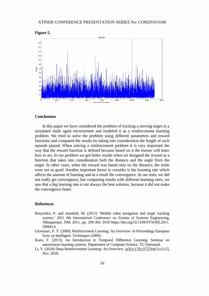
5. Id current distance > 22 or current distance < 18 then the reward is -10 and

the episode is finished; otherwise the reward is +1.The learning rate is 0.6,

Γ = 0.85 and there are 7500 episodes played. Figure 5 shows the results.

Figure 3.

Figure 4.


16

Figure 5.

Conclusions

In this paper we have considered the problem of tracking a moving target in a

simulated multi agent environment and modeled it as a reinforcement learning

problem. We tried to solve the problem using different parameters and reward

functions and compared the results by taking into consideration the length of each

episode played. When solving a reinforcement problem it is very important the

way that the reward function is defined because based on it the learner will learn

how to act. In our problem we got better results when we designed the reward as a

function that takes into consideration both the distance and the angle from the

target. In other cases, when the reward was based only on the distance, the reslts

were not as good. Another important factor to consider is the learning rate which

affects the amount of learning and as a result the convergence. In our tests, we did

not really get convergence, but comparing results with different learning rates, we

saw that a big learning rate is not always the best solution, because it did not make

the convergence faster.

References

Benavidez, P. and Jamshidi, M. (2011) "Mobile robot navigation and target tracking

system," 2011 6th International Conference on System of Systems Engineering,

Albuquerque, NM, 2011, pp. 299-304. DOI=https://doi.org/10.1109/SYSOSE.2011.

5966614.

Glorennec, P. Y. (2000). Reinforcement Learning: An Overview. In Proceedings European

Sym. on Intelligent Techniques (2000).

Kunz, F. (2013). An Introduction to Temporal Difference Learning. Seminar on

autonomous learning systems. Department of Computer Science. TU Darmstad.

Li, Y. (2018) Deep Reinforcement Learning: An Overview. arXiv:1701.07274v6 [cs.LG],

Nov. 2018.

https://arxiv.org/abs/1701.07274v6


17

Lund, H. H., Ves Cuenca, E., Hallman, J. (1996) A Simple Real- Time Mobile Robot

Tracking System. Techincal Paper no. 41, Department of Artificial Intelligence,

University of Edinburgh, 1996.

Luo, W., Sun, P., Zhong, F., Liu, W., Zhang, T., Wang, Y., (2018). End-to-end Active

Object Tracking via Reinforcement Learning. In Proceedings of the 35th International

Conference on Machine Learning, Stocholm, Sweden, 2018. arXiv:1705.10561

[cs.CV].

Mazo, M., Speranzon, A., Johansson, K. H. and Xiaoming. H., (2004) "Multi-robot

tracking of a moving object using directional sensors," IEEE International Conference

on Robotics and Automation, 2004. Proceedings. ICRA '04. 2004, New Orleans, LA,

USA, 2004, pp. 1103-1108 Vol.2. DOI= https://doi.org/10.1109/ROBOT.2004.13079

72.

Mnih, V., Kavukcuoglu, K., Silver, D., Graves, A., Antonoglou, I., Wierstra, D., &

Riedmiller, M.A. (2013). Playing Atari with Deep Reinforcement Learning.

arXiv:1312.5602 [cs.LG].

Mnih, V., Kavukcuoglu, K., Silver, D., Rusu, A. A., Veness, J., Bellemare, M. G., Graves,

A., Riedmiller, M., Fidjeland, A. K., Ostrovski, G., Petersen, S., Beattie, C., Sadik, A.,

Antonoglou, I., King, H., Kumaran, D., Wierstra, D., Legg, S. & Hassabis, D. (2015).

Human-level control through deep reinforcement learning. Nature, 518, 529--533.

DOI=https://doi.org/10.1038/nature14236.

Pinciroli, C., Trianni, V., O’Grady, R., Pini, G., Brutschy, A., Brambilla, M., Mathews, N.,

Ferrante, E., Di Caro, G., Ducatelle, F., Birattari, M., Gambardella, L. M., Dorigo. M.,

(2012). ARGoS: a Modular, Parallel, Multi-Engine Simulator for Multi-Robot

Systems. Swarm Intelligence, volume 6, number 4, pages 271-295. Springer, Berlin,

Germany. DOI=https://doi.org/10.1007/s11721-012-0072-5.

Ren, Liangliang & Lu, Jiwen & Wang, Zifeng & Tian, Qi & Zhou, Jie. (2018). Collaborati-

ve Deep Reinforcement Learning for Multi-object Tracking: 15th European Conferen-

ce, Munich, Germany, September 8–14, 2018, Proceedings, Part III. DOI=https://doi.

org/10.1007/978-3-030-01219-9_36.

Riedmiller M. (2005) Neural Fitted Q Iteration – First Experiences with a Data Efficient

Neural Reinforcement Learning Method. In: Gama J., Camacho R., Brazdil P.B.,

Jorge A.M., Torgo L. (eds) Machine Learning: ECML 2005. ECML 2005. Lecture

Notes in Computer Science, vol 3720. Springer, Berlin, Heidelberg. DOI=https://doi.

org/10.1007/11564096_32.

Sankar S, Tsai C-Y. (2019). ROS-Based Human Detection and Tracking from a Wireless

Controlled Mobile Robot Using Kinect. Applied System Innovation. 2019; 2(1):5;

DOI=https://doi.org/10.3390/asi2010005.

Sutton, R. S. and Barto, A. G. (2018) Reinforcement Learning: An Introduction (2nd

Edition, in preparation). MIT Press.

Tesauro, G. (1994). TD-Gammon, a Self-Teaching Backgammon Program, Achieves

Master-Level Play. Neural Computation, 6, 215-219. DOI= https://doi.org/10.1162/ne

co.1994.6.2.215.

Watkins, C.J.C.H. and Dayan, P. (1992) Mach Learn 8: 279. DOI=http://dx.doi.org/10.10

07/BF00992698.

Xiang, Y., Alahi, A., Savarese, S., (2015). "Learning to Track: Online Multi-object Trac-

king by Decision Making," 2015 IEEE International Conference on Computer Vision

(ICCV), Santiago, 2015, pp. 4705-4713. DOI=https://doi.org/10.1109/ICCV.2015.

534.

Zhang, D., Maei, H., Wang, X., & Wang, Y. (2017). Deep Reinforcement Learning for

Visual Object Tracking in Videos. arXiv:1701.08936[cs.CV].

https://arxiv.org/abs/1705.10561


https://doi.org/10.1007/s11721-012-0072-5



18

Zhong, Z., Yang, Z., Feng, W., Wu, W., Hu, Y., and Liu, C., (2019). "Decision Controller for

Object Tracking with Deep Reinforcement Learning," in IEEE Access, vol. 7, pp.

28069-28079, 2019.

Date post:	27-Nov-2021
Category:	Documents
Upload:	others
View:	3 times
Download:	0 times

ATINER CONFERENCE PRESENTATION SERIES No: …

Documents