THÈSE N O 2875 (2003) ÉCOLE POLYTECHNIQUE FÉDÉRALE DE LAUSANNE PRÉSENTÉE À LA FACULTÉ SCIENCES ET TECHNIQUES DE L'INGÉNIEUR Institut de traitement des signaux SECTION D'ÉLECTRICITÉ POUR L'OBTENTION DU GRADE DE DOCTEUR ÈS SCIENCES PAR enginyeria de telecomunicacions, ETSETB - UPC, Barcelona, Espagne et de nationalité espagnole acceptée sur proposition du jury: Prof. J.-P. Thiran, directeur de thèse Dr O. Cuisenaire, rapporteur Prof. B. Dawant, rapporteur Prof. M. Kunt, rapporteur Prof. G. Szekely, rapporteur Prof. J.-G. Villemure Lausanne, EPFL 2003 ATLAS-BASED SEGMENTATION AND CLASSIFICATION OF MAGNETIC RESONANCE BRAIN IMAGES Meritxell BACH CUADRA
Transcript
THÈSE NO 2875 (2003)
ÉCOLE POLYTECHNIQUE FÉDÉRALE DE LAUSANNE
PRÉSENTÉE À LA FACULTÉ SCIENCES ET TECHNIQUES DE L'INGÉNIEUR
Institut de traitement des signaux
SECTION D'ÉLECTRICITÉ
POUR L'OBTENTION DU GRADE DE DOCTEUR ÈS SCIENCES
PAR
enginyeria de telecomunicacions, ETSETB - UPC, Barcelona, Espagneet de nationalité espagnole
acceptée sur proposition du jury:
Prof. J.-P. Thiran, directeur de thèseDr O. Cuisenaire, rapporteurProf. B. Dawant, rapporteur
Prof. M. Kunt, rapporteurProf. G. Szekely, rapporteur
Prof. J.-G. Villemure
Lausanne, EPFL2003
ATLAS-BASED SEGMENTATION AND CLASSIFICATION OFMAGNETIC RESONANCE BRAIN IMAGES
Meritxell BACH CUADRA
A les meves arrels: els meusestimats avia, mare i germans.
When you set out on the voyage to Ithaca,pray that your journey may be long, full ofadventures, full of knowledge...
I present in this thesis the research work carried out during the last 4 years at the Signal ProcessingInstitute (ITS). Of course, this would not have been possible without the help of many people. Iwould like to thank them all.
Particularly, I would like to thank Prof. Murat Kunt who gave me the opportunity to join theITS and who has always followed my work with a lot of interest. My greatest thanks to my thesisadvisor Prof. Jean-Philippe Thiran who received me so kindly and gave me the opportunity to jointhe Computer Vision group. His enthusiasm has always been one of my greatest encouragements. Iam also grateful to all the members of my jury for their interest in reading and discussing my work.Special thanks to Prof. Benoit M. Dawant, for his precious comments that have always improved mywork. Also, I would like to gratefully acknowledge the enormous scientific support and friendship ofDr. Olivier Cuisenaire, who has co-directed my thesis. Merci Oli !
During these years I have strongly collaborated with many people. Particularly, it has been agreat pleasure to work with neurosurgeon Dr. Claudio Pollo. I have really appreciated his availabilityand medical knowledge. Many thanks to Torsten Butz, Eduardo Solanas, Mathieu De Craene, LeilaCammoun, Patric Hagmann, Valerie Duay and Olivier Ecabert for their valuable help. Specialthanks to the people at CHUV, Eleonora Fornari and Roberto Martuzzi, who have provided theimages. Also, many thanks to all my students, Anton, Martin, Julien, Val, Bram, Jesus, Olivier,Georg, for their motivating questions and precious work.
It has been a great satisfaction to work in the nice and familiar atmosphere that ITS peopleproduce: thanks to all the members! Special thanks to the members of the Computer Vision Group,for their support and complicity. I am also grateful to the secretaries of the laboratory, MarianneMarion, Fabienne Vionnet, Isabelle Bezzi and Corinne Degott, for their efficient work and patienceand also to Gilles Auric for his logistic support. Also, thanks to Nicolas Aspert and Diego SantaCruz for always helping me with Linux and LATEX. My gratitude goes also to all my estupendos officemates Andrea Cavallaro, Raphael Grosbois and Adel Rahmoune for their patience and kindliness.
I would like to thank also all the people in Lausanne that made my life so enjoyable during allthese years. Particularly, to Maria Eugenia and Ruth for all the great moments we spent togetherand the hours of discussions. My acknowledgment goes also to my old friends in Barcelona whohave always encouraged me. My greatest acknowledgement to the members of the Rodellar Gomezfamily for the support they have given me, specially to Bea and Neil for the professional correctionof my English mistakes of this manuscript.
Last, but not least, I would like to thank all the members of my family for their support andlove. Special thanks to my sister Anna who has come here many times to take care of me.
Finally, I would like to thank my love Dani for having always the strongest confidence in me.Thanks Dani for your unconditional love and friendship.
xiii
xiv Acknowledgments
Abstract
A wide range of different image modalities can be found today in medical imaging. These modalitiesallow the physician to obtain a non-invasive view of the internal organs of the human body, suchas the brain. All these three dimensional images are of extreme importance in several domainsof medicine, for example, to detect pathologies, follow the evolution of these pathologies, prepareand realize surgical planning with, or without, the help of robot systems or for statistical studies.Among all the medical image modalities, Magnetic Resonance (MR) imaging has become of greatinterest in many research areas due to its great spatial and contrast image resolution. It is thereforeperfectly suited for anatomic visualization of the human body such as deep structures and tissuesof the brain.
Medical image analysis is a complex task because medical images usually involve a large amountof data and they sometimes present some undesirable artifacts, as for instance the noise. However,the use of a priori knowledge in the analysis of these images can greatly simplify this task. Thisprior information is usually represented by the reference images or atlases. Modern brain atlasesare derived from high resolution cryosections or in vivo images, single subject-based or population-based, and they provide detailed images that may be interactively and easily examined in theirdigital format in computer assisted diagnosis or intervention. Then, in order to efficiently combineall this information, a battery of registration techniques is emerging based on transformations thatbring two medical images into voxel-to-voxel correspondence.
One of the main aims of this thesis is to outline the importance of including prior knowledge inthe medical image analysis framework and the indispensable role of registration techniques in thistask. In order to do that, several applications using atlas information are presented. First, the atlas-based segmentation in normal anatomy is shown as it is a key application of medical image analysisusing prior knowledge. It consists of registering the brain images derived from different subjectsand modalities within the atlas coordinate system to improve the localization and delineation ofthe structures of interest. However, the use of an atlas can be problematic in some particular caseswhere some structures, for instance a tumor or a sulcus, exists in the subject and not in the atlas. Inorder to solve this limitation of the atlases, a new atlas-based segmentation method for pathologicalbrains is proposed in this thesis as well as a validation method to assess this new approach. Resultsshow that deep structures of the brain can still be efficiently segmented using an anatomic atlaseven if they are largely deformed because of a lesion.
The importance of including a priori knowledge is also presented in the application of braintissue classification. The prior information represented by the tissue templates can be includedin a brain tissue segmentation approach thanks to the registration techniques. This is anotherimportant issue presented in this thesis and it is analyzed through a comparative study of severalnon-supervised classification techniques. These methods are selected to represent the whole range ofprior information that can be used in the classification process: the image intensity, the local spatial
xv
xvi Abstract
model, and the anatomical priors. Results show that the registration between the subject and thetissue templates allows the use of prior information but the accuracy of both the prior informationand the registration highly influence the performance of the classification techniques.
Another aim of this thesis is to present the concept of dynamic medical image analysis, in whichthe prior knowledge and the registration techniques are also of main importance. Actually, manymedical image applications have the objective of statically analyzing one single image, as for instancein the case of atlas-based segmentation or brain tissue classification. But in other cases the implicitidea of changes detection is present. Intuitively, since the human body is changing continuously,we would like to do the image analysis from a dynamic point of view by detecting these changes,and by comparing them afterwards with templates to know if they are normal. The need of suchapproaches is even more evident in the case of many brain pathologies such as tumors, multiplesclerosis or degenerative diseases. In these cases, the key point is not only to detect but also toquantify and even characterize the evolving pathology. The evaluation of lesion variations over timecan be very useful, for instance in the pharmaceutical research and clinical follow up. Of course, asequence of images is needed in order to do such an analysis.
Two approaches dealing with the idea of change detection are proposed as the last (but notleast) issue presented in this work. The first one consists of performing a static analysis of eachimage forming the data set and, then, of comparing them. The second one consists of analyzing thenon-rigid transformation between the sequence images instead of the images itself. Finally, bothstatic and dynamic approaches are illustrated with a potential application: the cortical degenerationstudy is done using brain tissue segmentation, and the study of multiple sclerosis lesion evolution isperformed by non-rigid deformation analysis.
In conclusion, the importance of including a priori information encoded in the brain atlases inmedical image analysis has been put in evidence with a wide range of possible applications. In thesame way, the key role of registration techniques is shown not only as an efficient way to combine allthe medical image modalities but also as a main element in the dynamic medical image analysis.
Version abregee
Dans le domaine de l’imagerie medicale il existe une grande variete de modalites d’images 3D qui per-mettent aux medecins d’obtenir une visualisation non invasive des organes du corps humain, commepar exemple du cerveau. Toutes ces modalites d’images sont tres importantes dans divers domainesde la medicine comme par exemple pour detecter certaines pathologies, pour suivre l’evolution desces pathologies, pour preparer et pour realiser des operations chirurgicales avec ou sans l’aide desystemes robotiques ou meme pour des etudes statistiques. Parmi toutes les modalites d’imagesmedicales, l’Imagerie par Resonance Magnetique (IRM) est devenue tres importante grace a sagrande resolution spatiale et son fort contraste pour les tissues mous. L’IRM est donc tres bienadaptee pour la visualisation anatomique du corps humain, par exemple des structures profondesou des tissus du cerveau.
L’analyse des images medicales est tres complexe car ces images sont representees par de grandesquantites de donnees et elles presentent parfois des effets non desirables comme le bruit. Cependantl’utilisation d’information a priori pendant le traitement d’images peut faciliter beaucoup leur anal-yse. Normalement, cette information a priori est representee par les images dites de reference ouatlas, qui determinent un espace commun ou l’anatomie humaine peut etre precisement represen-tee comme c’est le cas du cerveau. Aujourd’hui les atlas sont derives des images cryosectionees degrande resolution ou des images in vivo et ils sont bases sur un seul individu ou sur une populationd’individus. Dans tous les cas, elles fournissent des images tres detaillees qui peuvent etre facilementanalysees dans leur format digital pour des applications comme la vision et l’aide au diagnostic parordinateur. Finalement, il existe une grande variete des techniques de recalage basees sur des trans-formations qui donnent une correspondance voxel-a-voxel des images et qui permettent de combinertres efficacement toutes les informations contenues dans les images medicales.
Un des principaux objectifs de cette these c’est de souligner l’importance d’inclure dans l’analysedes images medicales l’information connue a priori et le role indispensable des techniques de recalage.Differentes applications qui utilisent l’information contenue dans des atlas sont presentees. Toutd’abord, la segmentation basee sur un atlas est presentee car c’est une application de pointe dansl’utilisation d’information a priori. Il s’agit de recaler des images du cerveau derivees des differentsindividus ou modalites d’image avec un atlas qui permettra d’ameliorer la localisation et segmen-tation des structures d’interet. Cependant, l’utilisation d’atlas et parfois limitee dans certains casou quelques structures, par exemple un sulcus ou une tumeur, sont presents dans le patient mais nesont pas presents dans l’atlas. On propose dans ce travail une nouvelle methode de segmentationbasee sur un atlas dans les cas de cerveaux pathologiques ainsi qu’une methode pour sa valida-tion. Les resultats montrent que les structures profondes du cerveau peuvent encore etre segmenteesefficacement a l’aide d’un atlas meme si elles ont ete largement deformees par une lesion.
La pertinence d’inclure l’information a priori est aussi presentee dans le cadre de la segmentationdes tissus principaux du cerveau. L’information contenue dans les atlas des tissus peut etre incluse
xvii
xviii Version abregee
dans la methode de classification du cerveau grace au recalage des images. Celle-ci est analysee gracea une etude comparative des diverses techniques de classification non supervisees. Les methodesetudiees ont ete selectionnees de facon a bien representer toutes les informations a priori qui peuventetre incluses: l’intensite de l’image, le modele spatial local, et les informations a priori anatomiques.Les resultats montrent que le recalage entre le sujet et les atlas des tissus permet l’utilisation desinformations a priori mais que la precision des deux, recalage et information a priori, influencefortement la qualite finale de la classification.
Un autre objectif de ce travail est de presenter le concept d’analyse dynamique des imagesmedicales, ou l’information a priori et les techniques de recalage jouent aussi un role important. Enfait, diverses applications de l’analyse d’image ont pour but d’etudier de facon statique une image.C’est le cas par exemple de la segmentation des images basee sur un atlas ou de la classificationdes tissus du cerveau. Mais dans d’autres cas, l’idee implicite de detection des changements estpresente. Intuitivement, comme le corps humain change continuellement, on voudrait faire uneanalyse de facon dynamique, c’est a dire, detecter quels sont les changements qui se sont produit et,en les comparant avec des informations a priori sur les changements, pouvoir detecter s’il s’agit dechangements normaux ou pathologiques. Le besoin de cette approche est encore plus evident dans lescas de certaines pathologies comme une tumeur, la sclerose en plaque ou les maladies degenerativesdu cerveau. Dans ces cas, l’objectif ce n’est pas seulement de detecter la pathologie mais aussi dela quantifier et meme de la caracteriser. L’evaluation des variations de certaines lesions tout aulong du temps permet d’avancer les recherches pharmaceutiques et un meilleur suivi clinique. Bienevidemment, de telles etudes ont besoin d’une sequence temporelle d’images du patient a traiter.
Deux approches differentes sont presentees afin d’illustrer cette idee de detection des change-ments. La premiere consiste a faire une analyse statique de chaque image de la sequence et decomparer apres les resultats. La deuxieme est basee sur l’analyse de la transformation non rigideutilisee pour deformer une image de la sequence vers une autre. Les deux approches sont presenteesa l’aide d’un exemple: l’etude de la degeneration du cortex du cerveau est fait grace a la segmenta-tion des tissus et l’etude de la sclerose en plaques est faite grace a l’analyse de la deformation nonrigide.
En conclusion, l’importance d’utiliser l’information a priori contenue dans des atlas dans ledomaine de l’analyse d’images medicales est presentee ainsi que ses applications. De meme, le roledecisif des techniques de recalage n’est pas seulement presente comme une facon efficace de combinerles differents types d’images mais aussi comme un element principal dans les approches d’analysedynamiques des images medicales.
Resumen
Hoy en dıa existen muchas modalidades de imagenes medicas digitales que permiten a los medicosel estudio in vivo de los organos del cuerpo humano, como por ejemplo del cerebro. Estas imagenesson muy utiles en muchos campos de la medicina como por ejemplo en la deteccion, seguimientoy estudio de patologıas, en la preparacion y realizacion de operaciones quirurgicas asistidas porordenador o en estudios estadısticos. De entre todos los tipos de imagenes medicas, destaca laimagen de Resonancia Magnetica (RM) por su alta resolucion espacial, su gran variedad de posiblescontrastes y su inocuidad al no utilizar radiacion ionizante. Estas caracterısticas hacen que la imagenpor RM sea muy adecuada para la visualizacion anatomica del cuerpo humano, por ejemplo paravisualizar las estructuras y los tejidos del cerebro.
El analisis de imagenes medicas es una tarea compleja ya que normalmente estas imagenesconsituyen grandes volumenes de datos y, ademas, presentan ruido y otros artefactos de la imagencomo los cambios de iluminacion. Sin embargo, la inclusion de informacion a priori en el analisisde estas imagenes puede facilitar mucho su estudio. La informacion a priori esta normalmenterepresentada por las imagenes de referencia o atlas que determinan un espacio concreto en el cualse describe la anatomıa, por ejemplo, del cerebro humano. Actualmente los atlas del cerebro (creadosa partir de secciones criogenicas o de imagenes in vivo, basados en un solo sujeto o en toda unapoblacion) proporcionan imagenes digitales muy detalladas que pueden ser examinadas interactivay facilmente en el diagnostico de tratamientos y planificacion de los mismos por ordenador. Enconsecuencia, para poder combinar de manera eficiente toda la informacion contenida en los distintostipos de imagenes medicas surgen las tecnicas de registro∗ que proporcionan las transformacionesgeometricas que situan dos imagenes en correspondencia anatomica voxel a voxel.
Uno de los objetivos principales de esta tesis es remarcar la importancia de incluir informaciona priori en el proceso de analisis de imagenes medicas ası como resaltar el papel indispensable delos metodos de registro en este proceso. Para demostrarlo, presentamos distintas aplicaciones queutilizan atlas. Primero, presentamos la aplicacion de segmentacion basada en atlas en sujetos conanatomıa normal ya que es una de las aplicaciones principales que incluyen informacion a priori. Lasegmentacion basada en atlas consiste en registrar una o varias imagenes del cerebro en el sistemade referencia del atlas para facilitar la localizacion y segmentacion de las estructuras de interes.Sin embargo, el uso del atlas esta limitado en algunos casos donde puede haber estructuras, comoun tumor o un sulcus, que esten presentes en el paciente pero no en el atlas. Para solventar esteproblema, se propone un nuevo metodo de segmentacion basado en atlas para cerebros patologicosası como un metodo para su validacion. Los resultados obtenidos demuestran que las estructurasde interes del cerebro se pueden segmentar utilizando la informacion contenida en un atlas aunqueesten muy deformadas debido a una lesion.
∗Anglicismo de registration.
xix
xx Resumen
La importancia de la utilizacion de la informacion a priori se demuestra tambien en la clasificacionde los distintos tejidos del cerebro. La informacion a priori contenida en los atlas de tejidos delcerebro puede ser utilizada por los metodos de clasificacion gracias al registro de imagenes. Esta estambien una aplicacion importante y se presenta a traves del estudio comparativo de varias tecnicasde clasificacion no supervisadas. Los metodos de clasificacion analizados han sido elegidos de maneraque representen la diversidad de informacion a priori que se puede utilizar, es decir, la intensidad dela imagen, la informacion local espacial y la informacion global contenida en los atlas. Los resultadosobtenidos demuestran que el uso de atlas es posible gracias a las tecnicas de registro pero que lacalidad de la clasificacion depende mucho de la precision del metodo de registro y de la calidad dela informacion a priori utilizados.
El tercer objetivo de esta tesis es presentar el concepto de analisis dinamico de las imagenesmedicas, en el cual, la informacion a priori y los metodos de registro siguen siendo de muchaimportancia. En realidad, muchas aplicaciones de las imagenes medicas tienen como objetivo elanalisis estatico de una imagen como, por ejemplo, en el caso de la segmentacion basada en atlaso en la clasificacion de tejidos del cerebro. Pero en otros casos la idea de deteccion de cambioses implıcita. Intuitivamente, ya que en el cuerpo se producen cambios continuamente, podrıamosanalizar las imagenes medicas desde un punto de vista dinamico, es decir, detectando los cambios quese producen y comparandolos con modelos de cambios para determinar si son normales. La necesidadde deteccion de cambios es aun mas evidente en el estudio de ciertas patologıas del cerebro como porejemplo tumores, esclerosis multiple o enfermedades degenerativas. En estos casos, la clave esta nosolo en detectar sino tambien en cuantificar e incluso caracterizar la evolucion de la lesion. Este tipode estudios pueden ser muy utiles por ejemplo en la investigacion farmaceutica o en el seguimientoclınico. Evidentemente, para realizar este tipo de estudios evolutivos se considera que se dispone deuna secuencia de imagenes a distintos intervalos de tiempo.
Dos metodos distintos que lidian con la idea de deteccion de cambios son presentados en estatesis. El primero consiste en realizar el analisis estatico de cada una de las imagenes que formanla secuencia y luego comparar los resultados. El segundo metodo consiste en realizar el analisisde la transformacion obtenida entre las imagenes de la secuencia, en vez de realizar el analisis decada imagen. Finalmente, presentamos una aplicacion potencial de cada uno de los metodos comoejemplo: el estudio de la degeneracion cortical del cerebro que esta hecho a partir de la clasificacionde tejidos y el estudio de la evolucion de esclerosis multiple que esta hecha a partir del analisis dela transformacion obtenida por registro.
En conclusion, se ha puesto en evidencia la importancia de considerar la informacion a prioride los atlas anatomicos del cerebro en el analisis de imagenes medicas en una gran variedad deaplicaciones. De la misma manera, el papel decisivo de los metodos de registro ha sido presentadono solo como una manera eficiente de combinar las distintas modalidades de imagenes medicas sinotambien como un elemento importante en el analisis dinamico de las mismas.
Resum
Avui en dia podem trobar una gran varietat de modalitats d’imatges mediques que permeten l’estudiin vivo dels organs del cos huma. Aquestes modalitats d’imatge son de gran utilitat en diversos campsde la medicina com per exemple en la deteccio, seguiment i estudi de patologies, en la preparacio irealitzacio d’operacions quirurgiques assistides, o no, per ordinador o en estudis estadıstics. D’entretotes les modalitats d’imatge destaca la Resonancia Magnetica (RM) per la seva alta resolucioespacial, contrast d’intensitat i la seva innocuıtat, ja que no utilitza radiacio ionitzant. Totes aquestescaracterıstiques fan que la RM sigui molt adequada per a la visualitzacio del cos huma, per exempleper a visualitzar les estructures i els teixits del cervell.
L’analisi d’imatges mediques es, pero, complexa ja que normalment les imatges estan formadesper grans volums de dades i presenten soroll i d’altres artefactes com els canvis d’il·luminacio. Ambtot, la introduccio d’informacio a priori en l’analisi d’imatges mediques pot facilitar enormementaquesta tasca. En molts casos aquesta informacio a priori esta continguda en les anomenades imatgesde referencia, o atles, les quals determinen un espai concret on es pot representar l’anatomia humana,com per exemple, l’anatomia del cervell. Actualment els atles del cervell (creats a partir d’imatgescriogeniques o in vivo, basats en un sol individu o en tota una poblacio) proporcionen imatges digitalsmolt detallades que poden ser examinades interactivament i facilment en el proces de diagnosi iplanificacio de tractaments per ordinador. Consequentment, per poder combinar eficientment totesaquestes informacions contingudes en les diferents modalitats d’imatge, emergeixen les tecniques deregistre∗ que tenen com a objectiu trobar la transformacio geometrica que situa dues imatges encorrespondencia anatomica voxel a voxel.
Un dels principals objectius d’aquesta tesi es demostrar la importancia de considerar la informacioa priori en l’analisi d’imatges mediques aixı com ressaltar el paper indispensable de les tecniques deregistre en aquesta analisi. Per demostrar-ho, diferents aplicacions mediques on s’utilitzen els atlesson estudiades en el marc de l’analisi d’imatges. En primer lloc presentem la segmentacio basadaen atles ja que es una de les aplicacions destacades de la utilitzacio de la informacio a priori. Lasegmentacio basada en atles consisteix en alinear el sistema de referencia de l’atles amb el d’unao varies imatges del cervell per facilitar-ne la localitzacio i delineacio de les estructures d’interes.L’us de l’atles queda, pero, limitat en els casos on algunes estructures, com per exemple un tumoro un solc, poden existir en l’individu i no en l’atles. Per resoldre aquest problema, proposem unnou metode de segmentacio basada en atles en el cas de cervells patologics aixı com un metodede validacio. Els resultats obtinguts demostren que les estructures d’interes es poden segmentarutilitzant un atles encara que estiguin molt deformades per culpa d’una lesio.
La importancia de la utilitzacio de la informacio a priori es demostra tambe en la classificaciodels diferents teixits del cervell. La informacio a priori continguda en els atles de teixits cerebrals
∗Anglicisme de registration
xxi
xxii Resum
pot ser introduıda en els metodes de classificacio gracies al registre d’imatges. Aquesta es una altraaplicacio important de l’us d’informacio a priori i la presentem a traves d’un estudi comparatiude diversos metodes de classificacio no supervisats. Els metodes analitzats han estat escollits demanera que representen el ventall d’informacio a priori disponible, es a dir, la intensitat de laimatge, la informacio espacial local i la informacio espacial global continguda en els atles. Elsresultats obtinguts demostren que la qualitat final de la classificacio depen molt de la precisio delmetode de registre i de la qualitat de la informacio utilitzats a priori.
El tercer objectiu principal d’aquesta tesi es presentar el concepte d’analisi dinamica de lesimatges mediques, en el qual la informacio a priori i els metodes de registre segueixen sent de moltaimportancia. Hem vist que algunes aplicacions de l’analisi d’imatges mediques tenen com a objectiul’estudi estatic d’una imatge, com es el cas de la segmentacio basada en atles o de la classificacio delsteixits del cervell. Pero en d’altres casos, la idea de deteccio de canvis es implıcita. Intuıtivament,ja que el cos huma canvia contınuament, les imatges mediques es podrien analitzar tambe des d’unpunt de vista dinamic, es a dir, detectant els canvis que es produeixen en una sequencia d’imatgesi comparant-los amb un patro de canvis per saber si son normals o patologics. La necessitat de ladeteccio de canvis es encara mes evident en el cas de certes patologies del cervell com per exemple untumor, l’esclerosi multiple o d’altres patologies degeneratives. En aquests casos, la clau no es nomesdetectar sino tambe quantificar i fins i tot caracteritzar l’evolucio de la lesio. L’estudi evolutiu potser de molta utilitat per exemple en la recerca farmaceutica o en el seguiment clınic. Evidentment,per a realitzar aquest tipus d’estudi es considera que una sequencia d’imatges a diferents intervalsde temps es disponible.
En aquesta tesi son presentats dos metodes diferents que tracten la idea de deteccio de canvis. Elprimer consisteix a realitzar l’analisi estatica de cada una de les imatges de la sequencia i, despres,a comparar-ne els resultats. El segon metode consisteix a realitzar l’analisi de la transformacioobtinguda gracies al registre de les imatges de la sequencia, en comptes de realitzar l’analisi estaticade cada imatge. Finalment, presentem una aplicacio potencial de cada un dels metodes com aexemple il·lustratiu: l’estudi de la degeneracio del cortex cerebral es fa a partir de la classificaciodels teixits del cervell i l’estudi de l’evolucio de l’esclerosi multiple es fa a partir de l’analisi de latransformacio obtinguda en el registre d’imatges.
En conclusio, s’ha demostrat la importancia d’incloure la informacio a priori continguda en elsatles del cervell en varies aplicacions de l’analisi d’imatges mediques. Aixı mateix, hem presentatel paper clau dels metodes de registre, no nomes com una manera eficac de combinar les diferentsmodalitats d’imatge, sino tambe com un element important de l’analisi dinamica d’aquestes.
Introduction 1Questa e una storia semplice,ma non e facile da raccontare.Giosue Orefice, ”La Vita e bella”(1997).
1.1 Motivation
Nowadays, different modalities of images can be found in medical imaging that allow us to obtaina non-invasive view of the internal organs of the human body, such as the brain. All these threedimensional image modalities are of extreme importance in several domains of medicine, for example,to detect pathologies, follow the evolution of these pathologies, prepare and realize surgical planningwith, or without, the help of robot systems or for statistical studies. The different types of medicalimages do not exclude each other, on the contrary, they usually contain complementary informationeven within the same modality.
Among all the medical image modalities, Magnetic Resonance Imaging (MRI) has recently be-come of great interest in many research areas. MRI creates a 3D image of the object under study,exploiting the magnetic properties of the water (hydrogen) contained in the human body. Thanksto its great spatial and contrast image resolution, MR images are perfectly suited for anatomicvisualization of the human body such as deep structures and tissues of the brain, the neck, theheart, the breast, etc. Also, MRI has the advantage over other medical image modalities that itdoes not use ionizing radiation. However, it also presents some limitations. For instance, a MRexam cannot be performed on patients with metallic devices such as pacemakers or with patientswho are claustrophobic (although new MRI systems are more open).
The analysis of medical images is a complex task because they usually involve a large amountof data and they present sometimes some undesirable artifacts, as for instance the noise. However,the use of prior knowledge on the medical image analysis can greatly simplify this task. This priorinformation is usually represented by the reference or atlases. Modern brain atlases derived fromhigh resolution cryosections or in vivo images, single subject-based or population-based, providedetailed images and may be interactively examined in their digital format. These new digitized
1
2 Chapter 1. Introduction
brain atlases try to overcome the earlier textbook limitations and their main advantages are thatthey provide a lot of detail and may easily be used in computer assisted diagnosis or intervention.
The brain warping or registration techniques are a battery of methods and algorithms thatemerges in order to efficiently combine all these different sources of information. They consistof finding the transformation that brings two medical images into voxel-to-voxel correspondence.Many variables participate in the registration paradigm and they allow many ways of classifying theregistration techniques. For instance, the warping methods can be divided into global or local trans-formations. Global transformations are typically applied to compensate for the different positionbetween two acquisitions (rotation, translation, scaling and shearing). Local registration is usuallyapplied to capture or compensate for the morphological variability in brain anatomy by performinga real deformation. However, many local registration methods require a global transformation asinitialization steps that makes the registration process a tandem of both types of transformations.
Thanks to the registration algorithms, the brain images derived from different subject and modal-ities can be for instance placed within the atlas coordinate system to improve localization anddelineation of structures, enabling correlations between individuals and modalities. Thus, digitalatlases may be used to calculate and provide morphometry and morphological measurements withina precise anatomical framework by mapping the template onto the target image. In the same way,population-based templates provide a representation of the human diversity neuroanatomy. Then,these templates can be used to detect and measure possible abnormal neuroanatomies.
1.2 Aims of this thesis
The first aim of this thesis is to outline the importance of including reference imaging in the med-ical image analysis framework. The application of atlas-based segmentation in the case of normalanatomy is presented as it is one important application of medical image analysis using prior knowl-edge. Then, the problem of using the anatomical atlas in the case of pathological anatomy arises.Thus, the second aim of this thesis is to efficiently segment deep structures of the brain using ananatomical atlas even if they are largely deformed because of a lesion. In order to do that a newatlas-segmentation method for pathological brains is proposed as well as a validation method toassess this new approach.
The effect of including a priori knowledge is also shown in the case of brain tissue segmentationthrough a comparative study of several classification techniques. The third goal of this work is toquantify the influence of prior information on the performance of several classification techniques.The methods presented in this validation are selected to represent the whole range of prior informa-tion that can be used in the classification: the voxel intensity, the local spatial model, and the priortemplates.
Finally, the fourth aim of this work is to present the concept of dynamic medical image analysis,in which prior knowledge and registration techniques are also of major importance. The idea is toanalyze and quantify the anatomy changes since the human body is in continuous motion. Twodifferent approaches dealing with the idea of changes detection are proposed and they are illus-trated by two potential applications: the cortical degeneration study is done using the brain tissuesegmentation, and the study of multiple sclerosis evolution is performed by non-rigid deformationanalysis.
1.3 Main contributions
The main contributions of this thesis can be summarized as follows:
1.4. Organization of the text 3
• A complete analysis of the demons algorithm input parameters.
• A new atlas-based segmentation approach of deep structures in pathological brains using amodel of tumor growth.
• A new validation method of the proposed model of lesion growth.
• Validation of brain tissue classification techniques using a whole range of prior information,i.e. intensity, spatial and anatomical priors.
• A new approach for localizing and quantifying gray mater degeneration using a 5 tissue clas-sification technique.
1.4 Organization of the text
This dissertation is organized as follows. First, Chapter 2 and Chapter 3 present the backgroundof this thesis. An overview of the existing medical image modalities is introduced in Chapter 2.Among these modalities, special attention is paid to MR imaging and to the digitized brain atlassince these two types of images are the objet of the research presented here. Then, in Chapter 3,the registration problem and its basic theoretical concepts are presented. Focus on the non-rigidregistration techniques is done and special attention is paid also to the demons algorithm that isdescribed in detail because it is the warping technique used in this work. Second, Chapter 4 andChapter 5 presents the atlas-based segmentation of deep brain structures. In Chapter 4, the solutionsovercoming the main limitations of the demons algorithm are presented and the choice of its inputparameters is discussed. Then, an example of atlas-based segmentation of normal anatomy is shown.The problem of using a priori information to register pathological brains is presented in Chapter 5.A new atlas-based segmentation method is proposed that tries to overcome the limitations of theexisting solutions. Also, a new validation method to assess the final segmentation is proposed.Third, the brain tissue segmentation process is presented in Chapter 6 through comparative studyof some of the most commonly used approaches. These methods were selected to represent thewhole range of prior information that can be used in the tissue classification, i.e. intensity, spatialand prior templates. Fourth, the concept of evolution study in medical image analysis is presentedin Chapter 7. Two different approaches leading with the study of changes are presented and theyare illustrated with two different applications: the gray mater degeneration study is done usingthe brain tissue segmentation, and the study of multiple sclerosis evolution is performed by non-rigid deformation analysis. Fifth, general conclusions and an outline of some future directions arepresented in Chapter 8. Finally, complementary information is given in the annex of this dissertation.Appendix A presents the general notation and Appendix B shows how the Maximum a Posteriori(MAP) classification is done when using a Markov Random Field.
4 Chapter 1. Introduction
Part I
Background
5
Brain imaging 2- I haven’t got a brain... only straw.- How can you talk if you haven’t got a brain?- I don’t know... But some people without brainsdo an awful lot of talking... don’t they?Scarecrow and Dorothy, ”Wizard of Oz ”(1939).
2.1 Introduction
Many image modalities can be used in medical image analysis. This chapter presents a brief overviewof these images focusing on brain imaging. Then, the basic principles of magnetic resonance imagingand state of the art of the reference imaging are explained in more detail within this framework sincethese are the image modalities used in this thesis.
2.2 Brain image modalities: an overview
There exists a wide range of 3D medical image modalities that allow neuroscientists to see insidea living human brain. This 3D brain imaging allows, for instance, to better localize specific areasinside the brain and to understand the relationships between them. Brain imaging can be dividedinto three main groups: anatomical, functional and reference imaging.
Anatomical imaging allows the study of the anatomical structures of the head such as thebones or the different brain tissues. For instance, the Computed Tomography (CT) scan uses a seriesof X-ray beams passing through the head, followed by a tomographic reconstruction, to build a 3Dimage of the head where bones and soft tissues are clearly identified. Magnetic Resonance (MR)imaging provides also an anatomical view of the tissue and deep structures of the brain thanks tothe magnetic properties of the water contained in the human body (a detailed description of MRimaging is presented in section 2.3). Diffusion tensor MR brain imaging is a relatively new imagemodality that permits in vivo measures of the self-diffusion properties of water in living tissues [8].This measure becomes highly anisotropic and oriented in areas of compact nerve fiber organization
Table 2.1: Classification of anatomical image modalities in function of the visualized structures.
MR CT Angiography Ultrasound
Figure 2.1: Anatomical Brain Images. MRA is from http://radi.med.hokudai.ac.jp. Ultrasound isfrom http://www.medphys.ucl.ac.uk.
of the brain providing an indirect way of white matter mapping and fiber tract identification [52, 64].Other anatomical images can be obtained, for instance, using MR or CT principles for Angiography(MRA or CTA respectively), that provide a 3D image of blood vessels. In between anatomical andfunctional imaging, there are CT and MR perfusion that are used to assess cerebral blood flow andblood volume in various brain regions. A contrast agent is injected and the volume of interest is thenscanned over time. Then, the resulting time series are processed to extent perfusion parameters.Finally, the echography generates an image by measuring the reflected sound waves of high frequency(hence, it is also called ultrasound imaging). Because high-frequency sound waves cannot penetratebone or air, this modality is specially useful in imaging soft tissues and fluid filled spaces. Echographyis thus quite often used in brain imaging, mainly in pediatrics and in blood vessels analysis. As seen,there is a large diversity of anatomical imaging and they are usually complementary to each other.For instance, in the case of radiotherapy, MR and CT are both necessary: the areas to treat arefirstly localized in the MR and the doses to use are then determined using the CT. However, MRIusually presents the best spatial and contrast image resolution and is perfectly suited for anatomicvisualization of deep structures of the brain.
Table 2.1 summarizes the above classification of anatomical imaging in function of the physicalsupport used in the acquisition process and in function of the structures that are better visualized.Figure 2.1 shows some examples of anatomical brain imaging.
Functional imaging allows the study of the brain activity by picturing the motor, sensoror cognitive tasks of the brain. Most of the functional imaging techniques can be classified intotwo major types of images: hemodynamic-metabolic and electric-magnetic [62]. Positron EmissionTomography (PET), Single Photon Emission Computed Tomography (SPECT) and Functional Mag-netic Resonance Imaging (fMRI) are included in the first group while Electroencephalography (EEG)and magnetoencephalography (MEG) belong to the second.
2.2. Brain image modalities: an overview 9
PET fMRSPECT EGG mapfMRI EGG mapPET SPECTsuperposed on an anatomical MRI
Figure 2.2: Functional Brain Images. SPECT is from http://webnt.physics.ox.ac.uk. EGG is fromwww.chasque.net.
PET and SPECT measure emissions from radioactively labelled chemicals, also known as tracers(e.g., fluoro-desoxy glucose FDG in PET), that have been injected into the bloodstreams. Thesetracers distribute over the body in a way that depends on its own properties and on the state of thebrain. Then, the 2D or 3D-image reconstruction of the distribution of these chemicals throughout thebrain is done. A particular tracer is used for each of the brain system or process to be studied. Forinstance blood flow, oxygen and glucose metabolism, protein synthesis, or drug concentrations canbe measured. Both PET and SPECT have the disadvantage of having low temporal resolution. PEThave more spatial resolution that SPECT though, particulary of deeper brain structures. SPECTstudies are longer since its tracers deteriorate more slowly than PET.
fMRI relies on the so-called Blood Oxygenation Level Dependent (BOLD) effect. Brain activationleads to changes in the concentration and ratio of deoxyhemoglobin within the activated region whichacts as an endogenous paramagnetic contrast agent. Indeed, increased blood flow reduces the localconcentration of deoxyhemoglobin causing an increase in the MR signal in a PD-weighted MRI (seeSection 2.3). The fMRI acquisition is faster than PET or SPECT and that allows greater precisionin determining active areas and how long the areas remain active: one image of brain activity persecond can be acquired with fMR imaging while PET studies take about 40 seconds or longer toacquire image brain activity. However, in some cases, the use of PET has some advantages overfMRI. For instance, in the case of auditive or language studies fMRI scans can be badly suitedbecause the gradient coils used in MR imaging are quite noisy. Also, since fMRI scans are moresensitive to the subject movement than PET, for some particular patient groups PET studies couldbe preferable than fMRI.
EEG and MEG use electrodes and sensors placed on the scalp to detect and measure patterns ofelectrical and magnetic activity emanating from the brain. Thus, they directly measure the neuronalactivity while PET, SPECT and fMRI rely on the induced physiology of the neurons activity. Theyhave greater temporal resolution than fMRI, PET or SPECT (they can record patterns of neuralactivity occurring within fractions of a second). However, its spatial localization is less precise thanfMRI and PET. Figure 2.2 shows some examples of functional brain imaging.
Reference imaging refers to all the a priori brain imaging information available. First, thetextbook brain atlas and, then, the digitized brain atlas compose the reference imaging. This imagemodality is extensively presented in section 2.4.
Table 2.2: Classification of functional brain image modalities. Either electric and magnetic fieldrefer to the ones generated by neural activity. rCBF denotes the regional cerebral blood flow.rCMRglc refers to the regional cerebral glucose metabolism. BOLD denotes the blood oxygenationlevel dependent effect.
2.3 Magnetic Resonance (MR) Imaging
Magnetic resonance imaging (MRI) creates a 3D image of the object under study exploiting NuclearMagnetic Resonance (NMR) phenomena and the magnetic properties of water (hydrogen) containedin the human body. In 1946, the NMR phenomenon was first observed independently by Bloch [12]and Purcell [91]. Then, in 1973, Lauterbur [68] generates the first MR images.
A brief introduction to the NMR phenomenon and the basic principles of the MRI formation arepresented. This overview is based on several documents as well as online sources [44, 56, 59, 78] towhich the interested reader can refer for more details.
2.3.1 Physical principles of MR imaging
Atomic nuclei with an odd number of protons (for instance, hydrogen nuclei) possess an intrinsiccharacteristic known as spin-angular momentum derived from the motion, or precession of thecharged particles. When a human body is placed in a large magnetic field (B0), many of the freehydrogen nuclei align themselves along or opposite to the magnetic field direction. The excessof spins create a net magnetic moment, M , parallel to B0. That is called polarization and thedirection along the polarization field B0 is known as longitudinal, z-axis, and the transverse plane isthe plane perpendicular to B0, xy plane. The hydrogen nuclei actually precess about the magneticfield direction like gyroscopes at a rate
ω0 = γB0, (2.1)
where the angular frequency ω0 is called Larmor frequency and it is proportional to the appliedmagnetic field strength by a gyromagnetic ratio, γ, characteristic of the atom being imaged (γ �42.6MHz/Tesla for hydrogen).
Then, a radio-frequency (RF) pulse, Brf , with a frequency ω0 is applied perpendicular to B0
and it causes M to tilt away from the polarization magnetic field. This effect is called resonance.When the RF pulse stops, the nuclei return to the equilibrium such that M is again parallel toB0. This behavior is known as relaxation. During this relaxation process, the nuclei lose energyand produces a RF signal, the free-induction decay (FID), that can be measured by an antennaor receiver coil. There are two interactions that describe this relaxation. One is the longitudinalrelaxation that results from“spin-lattice” interactions (T1) and the other is the transverse relaxationthat results from “spin-spin” interactions (T2), and results in an exponential decay of the transversemagnetization towards zero. Longitudinal and transverse relaxation are much slower effects thanprecession. For biological tissue the relaxation times vary from hundreds of microseconds to several
2.3. Magnetic Resonance (MR) Imaging 11
seconds. The differences in relaxation times (T1 and T2) and proton densities (PD) of different tissuetypes are exploited as a mechanism of generating contrast between different tissues in imaging, i.e.the voxel intensity that is visualized (see Fig. 2.3).
2.3.2 MR image formation
To produce a 3D image, the FID resonance signal must be encoded in each dimension. That isdone by applying a spatially linearly variable (stationary in time) magnetic field, B′
0 that inducesspatial distribution of the Larmor frequencies over the volume. Spatially constant derivatives of B′
0,(Gx, Gy, Gz), determine the local resolution of the image. The image reconstruction process can besummarized by three steps: selective excitation, phase encoding and frequency encoding. Selectiveexcitation applies a linear magnetic field that causes the Larmor frequencies to linearly change in thelongitudinal. Thus, a transversal plane can be selected by choosing the Brf frequency to correspondto the Larmor frequency of that plane or slice. Then, the 2D spatial reconstruction in each sliceis done by phase and frequency encoding. A linear field of gradient Gy is first applied causing theLarmor frequencies distribution to linearly vary according the y-direction. This causes a variationto the phase magnetization. When Gy is switched off, frequency returns to a constant value over theslice while phase remains proportional to y. Finally, a constant gradient Gx is applied perpendicularto Gy. Then, Larmor frequencies distribution linearly changes, this time according to the x-direction,while they still have a phase variation in y-direction. The resulting signal after successively applyingGz, Gy, and Gx corresponds to the Fourier transform of the transversal magnetization Mxy andproduces a single row in the spatial frequency space also known as k-space. After repeating thisprocess for different values of Gy a spatial matrix in the k-space is recovered and applying theinverse Fourier transform one slice of the MR image is obtained. The image volume is completed byrepeating this process for different values of the selective excitation frequency.
A typical 3D MRI data set is formed by 256 × 256 × 124 voxels with 0.9375 × 0.9375 × 1.5mm3
voxel resolution. Its acquisition in a 1.5 Tesla magnetic field can takes from 30 to 60 min.
2.3.3 Components of a MR imaging system
In summary, the MR system is composed by the following elements:
• a large magnet to create the magnetic field,
• shim coils to make the magnetic field as homogeneous as possible,
• a RF coil to transmit a radio signal into the body being imaged,
• a receiver coil to detect the returning radio signal,
• gradient coils to provide spatial localization of the signal,
• and a computer to reconstruct the radio signal into the final 3D image.
Figure 2.3 shows how an MRI scanner device looks like and the different MR modalities that canbe obtained: T1, T2 and PD weighted.
2.3.4 Clinical applications of MRI
MRI has the advantage over other medical image modalities that it does not use ionizing radiation.This modality is extensively used for medical visualization of most parts of the human body due toits high sensitivity for water. A few examples are enumerated in what follows.
12 Chapter 2. Brain imaging
Figure 2.3: Magnetic Resonance Imaging: MRI Scanner, MR-T1, MR-T2, and MR Proton Density.
• Brain MR is generally more precise for detecting brain abnormalities during the early stagesof a disease due to its high contrast between brain tissues. For instance, in the case of braintumors, the MRI will be positive before the CT does. Also, MR scans are very sensitive towhite matter diseases such as multiple sclerosis (MS). Other medical applications where MRI ispreferred are temporal lobe epilepsy, traumatic shear contusions, and gray matter degenerativedisease.
• MRI of the neck helps distinguish differences between lymph nodes and blood vessels. Itcan help detect tumors and other lesions, as well as vascular abnormalities, and structuralabnormalities.
• MRI is now able to utilize the blood as its own contrast agent to evaluate the blood vesselsof the head and neck. This technique is known as MR angiography (MRA). It can evaluateblood vessels of the head and neck without injecting the patient with a contrast agent. Thisnon-invasive technique requires only one additional set of pictures taken in addition with astandard MRI exam. MRA of the head and neck can help detect vessel narrowing (stenosis),blood vessel blockage, cerebral aneurysm, arteriovenous malformation (AVM), and blood vesseldissection.
However, MRI also presents some limitations. MR examinations cannot be used in patients withmetallic devices such as pacemakers or with patients who are claustrophobic (although new MRIsystems are more open). It is absolutely necessary that the patient not move during the acquisitiontime, thus, the patient must be able to be quiet during the exam period (from 20 to 60 min).
2.4 Reference imaging
As already presented in the introduction of this chapter, reference imaging involves the a prioriinformation available usually called atlas. The terms atlas and template represents the same reality:something that establishes a reference. Thus, a brain atlas is the abstract representation that servesas a pattern for comparing brains [55].
2.4.1 History of the brain atlases
The interest in brain anatomy and functionality started almost five millennia ago when an Egyptiansurgeon called Imothep described localization of brain function. After that, some philosophers andphysicians progressively discovered the motor, mental and sensory functions of the brain. In 1508A.D., first neuroatomical drawings were done by Leonardo da Vinci and few years later Vesalius
2.4. Reference imaging 13
presented the first complete study of human anatomy. Many other brain studies were carriedout but it is not until modern times that the first textbooks of brain function and anatomy wereproposed by Brodmann in 1909 [16], Talairach and Tournoux [106, 107] in 1957, and SchaltenbrandWahren [98] in 1977. A slice of Talairach and Tournoux textbook atlas is shown in Figure 2.4(a).These standardized atlases provide a precise common space in which to describe the anatomy of the
human brain. However, textbook atlases also present some limitations. For instance, they usuallycannot easily evolve and they are not usually compatible with each other. Digitized brain atlas tryto overcome these limitations and their advantage is that they provided a lot of detail and may beeasily used in computer assisted diagnosis or intervention.
2.4.2 Digitized brain templates
Many efforts have been recently made in order to digitize and compare some of the existing textbookatlas [86] as well as in the creation of digitized brain templates from high resolution cryosections [47]or in vivo medical images [37, 92]. Some of the existing computerized brain atlas are enumeratedin what follows. They are classified in two main groups: single subject and population-based atlas.A more detailed description is given for the atlases used in this work.
Single subject-based atlas
Cryosection-based atlas. One of the first digitized atlases was proposed by the Visible HumanProject [1] of the National Library of Medicine. Their goal is the creation of complete, anatomi-cally and detailed, three-dimensional representations of the normal male and female human bodiesby the acquisition of transverse CT, MR and cryosection high resolution images of representativemale and female cadavers. However, the frozen brain sections appear compressed and there is notmuch intensity contrast in the MR images since they scanned the brains after death. Also derivedfrom a digitized cryosectioned human brain, Greitz, Seitz, Thurfjell et al. [47, 102, 113] created aComputerized Brain Atlas (CBA) project that was designed for display and analysis of tomographicbrain images. The atlas includes the brain surface, the ventricular system and about 400 structuresand all Brodmann areas, that are outlined (see Figure 2.4(b)).
MRI-based atlas. Another type of atlas are those that are created from a MR image. Forinstance, the digital brain atlas developed by the Surgical Planning Laboratory (SPL) of Harvard
14 Chapter 2. Brain imaging
Medical School [92]. The template they proposed is a 3D MR digitized atlas of the human brainto visualize spatially complex structures. The MRI acquisition they used is from a single normalsubject and it has 256 × 256 × 160 voxels with 0.92 × 0.92 × 1.5mm3 per voxel. The manuallygeneration of anatomical labels finalize in 150 differentiated structures. Their work also includes 3Ddisplay tools. Figure 2.5 shows an axial view of the MRI, the corresponding labelled slice, and a 3Dview of deep brain structures (ventricles, thalamus and central nuclei). In what follows, this atlasis called SPL atlas.
Also, the digital brain phantom from McConell Brain Imaging Center [27] is based on 27 high-resolution scans of the same individual (1mm isotropic voxels low-noise). Then, a preprocessingwith non-uniformity reduction, an automatic segmentation (by minimum distance classifier), and,finally a manual correction of these scans was done. That resulted in a known classification: 103-dimensional ‘fuzzy’ tissue membership volumes where voxel values reflect the proportion of tissuepresent within the voxel. The Brainweb web-site also provides several simulated MRI acquisitions ofthis phantom including RF non-uniformities (bias of 0%, 20%, and 40%) and noise levels (0%, 1%,3%, 5%, 7%, and 9%). This makes them suitable for segmentation algorithm assessment. Figure 6.6shows an image with 5% of noise and 0% of inhomogeneities next to a 5- class ground truth classifiedimage created from the tissue membership volumes.
CT-based atlas. Bajcsy et al. [7] created an artificial CT anatomical volume based on thebrain sections taken from the Yakovlev Collection.
Population-based atlas
In principle, a single brain is not representative of a population. That is why population-basedatlases exploit the human brain variability in order to create a probabilistic brain atlas where thecross-subject anatomical and functional variations of a representative population are encoded. Afirst attempt of population-based model was presented by Hohne et al. in [60], where a frameworkfor generating an atlas from a collection of real volumes (MRI and a CT) was introduced. Woodset al. [121] created two average brain atlas in T1 and T2 from ten normal subjects registered intoa Talairach space. A composite MRI data set was constructed by Evans et al. [37] from severalhundreds of normal subjects (239 males and 66 females of 23.4 ± 4.1 years old). All the scanswere first individually registered into the Talairach coordinate system. Then, they were intensitynormalized and, finally, all the scans were averaged voxel-by-voxel. This average template is part ofthe widely used Statistical Parametric Mapping (SPM) package [39].
The population-based atlas are in continuous evolution since a new-subject can be easily incor-porated. Also, the population that a probabilistic atlas represents can be easily subdivided intogroups according to specific criteria (age, sex, handedness, etc). Recently, population-based atlasesare also based in representative subgroups of some disease, instead of using a healthy represen-tative group of subjects, that is, disease-based atlas. For instance, functional and morphologicalatlases for Alzheimer, Parkinson or Schizophrenic diseases are being of increasingly research inter-est [36, 81, 111, 116]. Such atlases would provide the way to examine the history and evolution (dueto natural disease evolution or reaction in front of a clinical treatment) of a specific disease.
2.4.3 Digitized brain atlas applications
Modern brain atlases derived from high resolution cryosections or in vivo images, single subject-based or population-based, provide detailed images and may be interactively examined in theirdigital format. Then, brain images derived from different subject and modalities can be placedwithin the atlas coordinate system to improve localization and delineation of structures, enabling
Table 2.3: Classification of reference brain imaging.
correlations between individuals and modalities. Thus, digital atlases may be used to calculate andprovide morphometry and morphological measurements within a precise anatomical framework bymapping the template onto the target image. Then, the resulting 3D transformation can be used todefine and quantify the brain morphology. In the same way, population-based templates provide arepresentation of the human diversity neuroanatomy. Then, these templates can be used to detectand measure possible abnormal neuroanatomies or, on the contrary, to keep new transformationsinside their space of normal anatomy.
2.5 Summary
In the last century, a rapid advance in neuroimaging produced important changes in clinical neu-roscience. There exist a large variety of image modalities that usually address a particular aspectof the underlaying physiology. However, among all the different brain images, complementary in-formation is usually provided even within the same image modality. In this chapter, basic conceptson anatomical, functional and reference brain imaging have been introduced. Focus on magneticresonance imaging and digitized brain atlases has been done since they form the data sets used inthis thesis.
The MRI principles have been first presented as well as the advantages of MRI versus other imagemodalities. For instance, MRI usually presents the best spatial and contrast image resolution and isperfectly suited for anatomic visualization of deep structures of the brain. There are however someexceptions where a MR exam cannot be considered. For instance, for patients having implanted ametallic device or claustrophobia a MR exam cannot be executed.
A wide discussion on the existing brain atlases presented two main group of digitized templates:single-based and population based. The importance of brain atlases has been put in evidence withtheir wide range of possible applications. All digitized templates have the same major advantage:anatomical and/or functional structures and large number of subjects can be automatically comparedto a brain atlas. However, their principle itself is its main limitation since templates are defined torepresent the anatomy of the majority of the individuals. Thus, they are used to compare similartopologies. But there are some cases where some structures, such as a tumor or minor sulci, arepresent in the subject but not in the template.
Now, an important question arises within all the brain image modalities: how to efficientlycombine all these different sources of information? A battery of methods and algorithms emerges inorder to answer this question: the brain mapping or registration techniques and they will be treatedin the next chapters.
16 Chapter 2. Brain imaging
(a) MRI. (b) Labels. (c) 3D view.
Figure 2.5: Digital brain atlas of the Surgical Planning Laboratory of Harvard Medical School: (a)Magnetic resonance of the atlas. (b) Atlas with all labelled brain structures. (c) 3D view of deepstructures of the brain: ventricles (green), central nuclei (red) and thalamus (blue).
(a) T1-MRI, 5% noise, 0% RF. (b) Ground truth classification.
Figure 2.6: Digital brain phantom from McConell Brain Imaging Center. (a) Brainweb phantomsimulated T1-MRI with 5% noise and 0% RF. (b) 5-class ground truth classification.
Figure 2.7: SPM probability maps of brain tissue.
Image Registration 3At night my mind would come alive with voices and stories.I gave myself up to it, longing for transformation.Jo, ”Little women”(1994).
3.1 Introduction
In this chapter the basic theoretical concepts of image registration are exposed focusing on non-rigidregistration techniques. First, a theoretical formulation and a general classification of registrationtechniques are presented. After that, a brief state of the art of non-rigid registration is done in orderto introduce the warping method used in this work that is described and analyzed in detail at theend of the chapter.
3.2 Medical image registration
There is a lot of information available in medical imaging. All this information can be efficient-ly combined by medical image registration: it consists of finding the transformation that bringstwo medical images into a voxel-to-voxel correspondence. Generally, the terms registration andmatching are both used to refer to any process that determines correspondence between data sets.
Many variables participate in the registration paradigm and they make the classification ofregistration techniques a difficult task. A wide overview of medical image registration is done in[53, 79, 118]. Maintz et al. present in [79] a survey of medical image registration techniques undernine different criteria. The more relevant criteria are also used here.
The main actors in the registration process are the brain images. Two images are matched oneto the other: the target image, also called reference image or scene (f), and the image that will betransformed, also called floating image or deformable model (g). If the images to register belong tothe same modality it is said to be monomodal registration and if they belong to different modalitiesit is said to be multimodal registration.
17
18 Chapter 3. Image Registration
We can also distinguish between intra-subject and inter-subject registration. In the first case,both reference and floating images belong to the same patient. The goal of intra-subject registrationis usually to compensate the different positioning of the patient in the acquisition process as wellas other possible geometrical artifacts of the images. This kind of registration is usually needed insurgical planning, lesion localization or pathology evolution. Some examples are the registration ofa CT and a MR image for radiotherapy or the registration of an anatomical MRI with a fMRI forlesion localization. In the second case, images are acquired from different patients or from a patientand a template image. The goal of this kind of registration is to compensate the inter-subjectanatomical variability in order to perform statistical studies or to profit from reference data, forinstance for surgical planning.
The image modalities to register and the application will determine the rest of the variables thatbelong to the registration process:
• the features to be matched,
• a cost function to minimize,
• the domain of possible transformations T ,
• and the evaluation of the results.
A more detailed classification of the registration techniques under the first three criteria follows.Validation is discussed at the end as conclusion of the chapter.
3.2.1 Features and cost function
Registration techniques can also be divided into voxel-based and into model-based techniques. On onehand, voxel-based approaches directly use voxel intensity. Some of them encode the image intensityinto a set of scalars and orientation (principal axes and moments-based registration). But most ofthe voxel-based registration approaches uses the whole image intensity (intensity-based registration)and, once a cost function is defined between the reference and the floating images, the transformationis successively adjusted until the cost is minimized.
On the other hand, model-based approaches are landmark-based or segmentation-based : iden-tifiable anatomical elements (point landmarks, lines or surfaces) are extracted in both referenceand floating image and their correspondence determine the volumetric transformation. They usehigh-level anatomical information (sulcal lines, functional surfaces, important point landmarks) andthat explicitly guarantees the physical validity required in the brain registration process. But theypresent also the disadvantage of having a previous feature extraction step (not always an automaticmethod can be used) and consequently the registration validity depends on the feature extractionaccuracy.
Of course, feature selection depends on the image modality and the definition of the cost functiondepends on the selected features. Usually,
Costfunction = −Similarity measure,
and this similarity measure can be intensity-based (voxel-based registration) or distance-based(model-based registration). Some similarity intensity measures are: normalized cross-correlation [6],absolute or squared intensity difference [24], measures based on optical flow concept [33], mutualinformation [19], etc. And some distance measures are: Procrustean metric [45], Euclidean dis-tance [29], curvature [30], etc.
3.2. Medical image registration 19
Figure 3.1: Domain and nature of a transformation. Figure extracted from [17].
3.2.2 Domain of transformation
Another possible classification criteria used in [79] is the nature and domain of the transformation.The nature of transformation is rigid (only translations and rotations are allowed), affine (parallellines are mapped onto parallel lines), projective (lines are mapped onto lines) or curved (lines aremapped onto curves). Then, the transformation domain can either be local or global. A transfor-mation is called global when a change in any one of the transformation parameters influences thetransformation of the image as a whole. In a local transformation a change in any transformationparameter only affects a part of the image.
According to Brown [17], the domain of the transformation is the main characteristic of any reg-istration technique. But the local-global paradigm can be attributed not only to the transformationitself but also to the computation domain. That is, the information on which the registration isbased and the similarity function domain can span from very local to very global. However, globalusually refers to rigid (6 parameters in 3D) and affine (12 parameters in 3D) registrations and weconsider curved registration as a local transformation. Curved registration is also called non-rigidregistration or warping (see section 3.3).
3.2.3 Registration problem formulation
The image registration problem can be formulated by the following minimization equation:
T ∗ = argminT∈T
cost(f, T ◦ g) (3.1)
Note that all transformations in T have to follow some physical constraints in order to model real-istic deformation between two brains (we can deform a brain into an apple but it is not very likely
Nature Rigid Affine Projective CurvedDomain Global Local
Table 3.1: Different registration techniques classification.
to happen). Global transformations defined by an analytical expression (rigid, affine or splines) usefew parameters and explicitly fulfill these physical constraints. The cost function in these cases isjust defined by a similarity criteria (either intensity or distance-based). But in more local trans-formations the complexity of the transformation might increase until a large number of parametersand they usually assure a physically valid transformation by adding to the similarity criteria a termrepresenting the allowed deformability (fluid models, elastic models or diffusion models):
Cost = Deformability − Similarity. (3.2)
To conclude the state of the art of registration techniques, Table 3.1 summarizes the possibleclassification under the selected criteria.
3.3 Non-rigid Registration
As seen before, the available image data and the final application of the registration process deter-mine the nature and domain of the transformation. Some possible needs of registration in medicalimaging could be:
• the analysis of functional imaging to locate functionally homologous brain regions,
• to remove position, inter-subject size and shape difference between the brain images for sta-tistical studies or a reference atlas construction,
• the atlas-based segmentation, that is, the registration between an atlas and a patient to auto-matically identify template structures into the subject brain,
• to localize, model and quantify the brain’s anatomical variability, in the healthy-to-healthy orthe healthy-to-pathological case.
All these applications have a common denominator: the need to capture the morphological variabilityin brain anatomy. That is why a global registration is not enough to finally obtain the desiredcorrespondence and a more local deformation is needed. However, many local registration methodsrequire a global transformation as initialization step that makes the registration process a tandem ofboth types of transformations. The registration methods that are neither rigid nor affine are namedhere non-rigid registration or warping.
There are among all the warping techniques several matching criteria and several types of trans-formation, thus there is not one hierarchy which is better than another. As for registration onlya few surveys exist in brain warping [73, 115]. The state-of-the-art presented here is limited to
3.3. Non-rigid Registration 21
intensity-based non-rigid registration techniques. All the existing techniques are summarized in twomain groups, parametric and non-parametric, in order to better identify the matching method usedin this work.
3.3.1 Parametric transformations
We have seen that global transformations (rigid or affine) are represented by few parameters. Thecomplexity increases up to hundreds of parameters for the local transformations: instead of usinga matrix or polynomial representation of the transformation, a linear combination of basis func-tions can be used. These methods are called here parametric warping techniques. For instance,trigonometric [4], wavelets [2] or splines could be used as basis functions. These methods are con-trol point-based, that is, the transformation is calculated at some points and the continuity of thetransformation at the rest of the image is ensured by an interpolation function∗. The number ofparameters is strictly dependent on the number of control points. The grid must be a regular one forsome basis functions such as B-splines [117] but may be non-uniform grid for radial basis functions(thin-plate splines [13], Gaussian, etc). However, the use of a non-regular distribution of controlpoints makes their choice a critical aspect of the registration process. These approaches have the ad-vantage of having a free choice of the cost function and many times the mutual information measureis used so multimodal data can be matched [66, 96].
3.3.2 Non-parametric transformations
In the extreme case one or more parameters per voxel can be used. This kind of registration is calledhere non-parametric transformations. Non-parametric transformations are usually defined by theirassociated displacement field
−→D (three coordinates per voxel in 3D) at each voxel position
−→P . The
transformation of one image by this vector field can be formulated as follows:
T ◦ g(−→P ) = g(T (
−→P )) = g(
−→P +
−→D(
−→P )). (3.3)
This is known as Lagrangian reference frame, i.e. deformations are defined with respect to the initialposition.
Elastic registration techniques have been introduced earlier by Bajcsy et al. [6] where imageregistration is treated as the physical deformation described by the stretching of an elastic material.Two forces drive this deformation: the internal and external forces. Internal forces are definedby the elastic properties of the deforming media (Lame’s elasticity constants) and they representthe deformability term of the cost function. External forces are the cost function similarity termand they actually drive the registration process. Usually, these forces are gradients of the chosensimilarity measure: cross-correlation [6], squared differences in pixel intensities[82] and a mix ofintensity and curvature and edge features[42]. The elastic registration problem is formulated bythe Navier linear elastic partial differential equation (PDE). It can be solved numerically by finitedifferences [30] or finite elements [38]. In these cases the regularity of the transformation is drivenby the laws of the continuum mechanics.
In order to allow more deformability than the elastic methods, Christensen et al. [24] pro-pose a transformation driven by a viscous-fluid model which allows non-linear topological behaviorwhile satisfying the laws of the continuum mechanics. In contrast to elastic registration techniques,viscous-fluid deformation is formulated in terms of the instantaneous field instead of the displace-ment field (in fact, deformation is here defined with respect to the final position, that is, the Eulerian
∗In a non-control point the transformation is defined by an analytical expression of the transformation computed
at the control points within the region of influence of the considered non-control point.
Table 3.2: Classification of the warping techniques.
reference frame). Two methods are proposed to solve the fluid PDE: using successive over relax-ation [24] or using spectral methods [15].
All the approaches presented can be seen as attractor techniques: where deformation forces areusually defined from the deformation model and directed towards the target image. In oppositionto these methods, Thirion [109] presents a different approach inspired by thermodynamics: thedemons-based algorithm. In this approach, the forces are originated from the scene and they aredirected inward or outward of the scene objects. The regularity of the transformation is ensured bya simple linear convolution of the deformation field with a separable filter. That makes the demonsalgorithm a fast warping algorithm. This is one of the reasons why this method has been chosen inthis work. A detailed description of this technique will follow in the next section.
3.4 Demons algorithm
J.Ph. Thirion introduces the image registration problem as a diffusion process [109, 110] based onan analogy with a thermodynamic concept (Maxwell’s demons) and on the optical flow estimation.A detailed analysis of this method is presented in the following sections since this is the non-rigidregistration method used in this thesis.
3.4.1 Optical Flow Concept
The optical flow is an estimation of motion [9] and it can be used in a wide range of applications suchas 3D scene analysis in robotics or virtual reality, motion image compensation in remote sensing orimage compression. The estimation problem can usually be seen as an object to track in a sequenceof images. The optical flow estimation is based on the following assumption: in an image sequence,the intensity of a real point does not change in time. The formulation of this assumption in the 2-Dcase is as follows:
I(x(t), y(t), t) = I(x(t0), y(t0), t0) = C, (3.4)
where (x, y) represents the spatial coordinates, I is the intensity, t is the index time, and C is aconstant. Taking the derivative with respect to the time, the above assumption can be rewritten as
∂I(x(t), y(t), t)∂t
=∂I
∂x
dx
dt+
∂I
∂y
dy
dt+
∂I
∂t= 0. (3.5)
Remark that the instantaneous speed of a point can be defined as:
−→v = (dx
dt,dy
dt). (3.6)
Then, equation 3.5 becomes−→∇I · −→v = −∂I
∂t, (3.7)
3.4. Demons algorithm 23
that is known as the optical flow equation and estimates the motion using both the spatial gradientand the temporal derivative of the image intensity. However, this equation formulates an ill-posedproblem since a scalar equation has to determine two unknowns, the two components of the speed−→v = (vx, vy). Actually, only the motion along the intensity gradient (object contours) can bedetermined while no access to the component along the object contours is available. This is calledthe aperture problem. An additional assumption is needed to solve this problem. The smoothestsolution is the regularization that supposes the component of the speed orthogonal to the gradient iszero and a regular optical flow in the whole image [61] and this is the one used here (see Section 3.4.5).Other possible solutions are the block matching which assumes the optical to be constant on smallwindows in the image [3] or the spatiotemporal filtering methods which rely on the assumption thatthe optical flow is constant over the support of their filters [26].
3.4.2 Demon points
Demon points are the features matched in the demon algorithm. Opposite to the attractor-basedmethods, in this approach the feature set is extracted from the scene image and not from thedeformable image. Several kind of demons can be defined. A grid of demons is considered here.All voxels where
−→∇I �= 0 are selected to be demons. In this case, the interface at each point is aniso-surface. Notice that in the case of medical imaging, and particulary MR images, the iso-surfacesrepresent the shapes of object, because the intensity in a MRI represents the different biologicaltissues. It is assumed that demon polarity can be determined. This assumption is easily fulfilledsince MR intensity gradient determines the normal to object contour, that is, the inside-outsideorientation. So, a demon should be understood as an intelligent agent that, being placed at a pointof the scene, pushes the deformable model in the normal direction of the scene contour∗. The formalexpression of this idea is:
Definition 1 (Regular grid of demons) Let f be the 3D image intensity function of the scene,and g be the 3D image intensity function of the deformable model. A demon is associated to eachvoxel P of the scene image where |−→∇f(P )| > ε, meaning that an iso-surface comes through voxel P ,whose implicit equation is f = f(P ), and whose oriented normal is
−→∇f(P ).
The threshold ε defines the type of demons and in this work is defined by the quantification step(ε = 0). A more detailed discussion about the choice of this threshold is presented in section 4.3.3.In summary, note that the information contained at each demon is:
1. the spatial position (−→P ),
2. the inside-outside polarity(−→∇f(
−→P )),
3. the current displacement (−→D(
−→P )),
4. and the intensity (f(−→P )).
∗Maxwell’s demons were introduced in physics to model the paradoxical idea that a semi-permeable membrane
could violate the second law of thermodynamics (about entropy). Situated in the membrane, those demons are
supposed to sort locally two different types of molecules of a mixed gas, to put one type on one side and the other
type on the other side of the membrane, hence giving a decrease in entropy. As each demon needs to consume some
energy to sort, the global entropy of the system is still increased, which suppresses the paradox.
Object boundaries in the scene image f are viewed as semi-permeable membranes. The floatingimage g is considered as a deformable grid, and diffuses through these interfaces driven by theaction of demons situated within the membranes. In the particular case of voxel-by-voxel intensitysimilarity, the demons paradigm is similar to optical flow methods: f and g are seen as two framesof a motion sequence, and the target is to find the motion vector −→v that brings g closer to f . Theassumption that there is a conservation of the intensity of points under motion is applied, whichcan be expressed as:
∂I
∂x
∂x
∂t+
∂I
∂y
∂y
∂t+
∂I
∂z
∂z
∂t= −∂I
∂t(3.8)
It can be considered that f and g are separated by only one unit of time: ∂I/∂t = f − g.The motion vector is defined as −→v = (∂x/∂t, ∂y/∂t, ∂z/∂t), and corresponds to the instantaneousvelocity from g to f . Therefore, the expression of the motion from g to f is:
−→v · −→∇f = g − f (3.9)
And, therefore the instantaneous velocity can be computed from the intensities of the scene andmodel images with the following expression:
∂I∂t = f − g−→v = (∂x
∂t , ∂y∂t , ∂z
∂t )−→∇f = (∂f
∂x , ∂f∂y , ∂f
∂z )
⇒ −→v =(g − f)
−→∇f
|−→∇f |2(3.10)
The expression above of the motion vector −→v could be used as demon’s pushing force, as thisforce would push inward (in the direction of
−→∇f) when f < g, and outward (toward −−→∇f) whenf > g, which is the desired behavior of a demon (see Figure 3.2). However, the expression inEquation (3.10) is unstable when the gradient norm is small, which would lead to infinite values ofthe pushing force for the regions having small variations of intensity. The desired behavior of thepushing force equation would be that the force should be given by Eq. (3.10) when the gradient ishigh, and close to zero when the gradient is low. J.-P. Thirion proposes multiplying the expressionin Eq. (3.10) by {−→∇f2/[
−→∇f2 + (g − f)2]}, which provides the desired effect of limiting the force to
3.4. Demons algorithm 25
finite values. Finally, the expression of the demons pushing force is:
−→v p =(g − f)
−→∇f
|−→∇f |2 + (g − f)2. (3.11)
Definition 2 (Demon forces) The demon in P pushes the deformable model image according to−→∇f(P ) if f(P ) < g(P ) and according to −−→∇f(P ) if f(P ) > g(P ). Hence, a whole 3D grid of demonsacts to deform the deformable model using the intensity gradient as direction of the deformation,and using the difference in intensity as orientation of the direction and magnitude.
In the particular case where f(P ) is equal to g(P ), the demon force in equation 3.11 is zero, i.e. thereis no displacement necessary since intensities are already matched. The instantaneous displacementof the non-demon points is also zero. Finally, note that relationship between demon force −→v p andthe instantaneous displacement
−→d is defined as
−→d = −−→v p.
3.4.4 Iterative process
As for attraction-based approaches, demons algorithm performs better in an iterative scheme. First,a computation of the demon points Pdemons in the scene f is done and, then, the iterative estimationof the total deformation field
−→D is done. At each iteration i, we have the current estimated deformed
field−→D i, and 2 steps are performed:
1. For each demon P ∈ Pdemons, the instantaneous deformation field is computed,−→d (P ), which
depends on the demon direction,−→∇f(P ), and on the polarity of g(P +
−→D i(P )) with respect
to f(P ).
2. Update−→D i+1 =
−→D i +
−→d (P ) and constrain it using the relations between the image model
voxels (see section 3.4.5).
Using this iterative approach the spatial influence of the demon points becomes less local but theassumption of small displacements is still considered. Now, the number of iterations should be de-termined and it is usually done empirically. An algorithm convergence study is done in section 4.3.5.
3.4.5 Regularization
Eq. (3.11) estimates demon displacements when considered separately. Thus, there is no constraintson the displacement field
−→D that ensures global smoothness of the transformation. The problem
is solved thanks to Tikhonov regularization theory [114] which looks for a differentiable function(deformation), which is, in some sense, closest to our signal (
−→D). There exist a wide range of
possible solutions, from simple linear regularization to complex non-linear physical models. Forsimplicity, Thirion proposes to deal with a linear regularization. Let us write it formally [83],
Definition 3 (Linear regularization) The Tikhonov regularized solution D of the signal D ∈L∈(�) is the one that minimizes the energy (E) functional
E[D] ≡ 12
∫dx((D − D)2 +
∞∑i=1
σi
i!(∂iD
∂xi)2). (3.12)
26 Chapter 3. Image Registration
Compute demon points in scene (f), {P demons}
Compute demon instantaneous displacements ( d )
Update total deformation field ( D )
Regularization
i
Figure 3.3: Iteration i of demons algorithm.
The solution of the regularization problem is the linear convolution of the signal D by the filter h,having the Fourier transform
G(w, σ) =1∑∞
i=0σi
i! ω2i= e−ω2σ, (3.13)
which is the well known Gaussian filter defined by its standard deviation σ (expressed in mm).Practically, the deformation field regularization becomes a discrete convolution. A fast separableimplementation is done by filtering consecutively each spatial direction by a vector of Gaussiandistributed weights∗.
Intuitively, demon algorithm can be seen as an elastic-like algorithm if the total displacementfield
−→D is filtered since elastic models smooth the elastic body displacements [21]. Inversely, if the
instantaneous vector field−→d is filtered, demon algorithm can be seen as viscous fluid-like since
viscous fluid models smooth the velocities of the fluid body.Then, the deformability of the algorithm is only modelled by the σ parameter of the Gaussian
filter (we also call it elasticity parameter). But this simplicity is both the strong and weak point ofthe algorithm since the choice of this parameter is a key aspect of the non-rigid registration processand it is however done empirically (see section 4.3.4).
3.4.6 Multiscale implementation
In order to make the algorithm more robust to large differences (these differences could render op-tical flow methods completely ineffective because the assumption of small displacement is violated),the deformation algorithm is applied in a hierarchical way. By hierarchical way we understand amultiscale implementation: a first match is made with downsampled images (coarsest scale) andthe resulting transformation is upsampled to initialize the next match with finer image resolution.Thus, the solution is refined from coarse-to-fine scales as represented in Fig. 3.4.
There are several advantages in using a hierarchical implementation. First notice that the samenumber of Gaussian filter coefficients are used at each scale. Then, the filter coefficients represent
∗Note that the weights of the discrete Gaussian filter are computed from σ in a way that the same number of filter
coefficients are used at each scale (see Section 3.4.6).
3.4. Demons algorithm 27
Scale 3
Scale 2
Scale 1
Scale 0
B r
a i
n
a
t l
a s
P a t i e n t
256x256x160 256x256x160
128x128x80 128x128x80
32x32x20 32x32x20
64x64x4064x64x40
I=16
I=32
I=64
I=128
Figure 3.4: Multiscale.
different voxel sizes for each scale, i.e. in the first scales we have a less elastic filtering (biggestmorphological differences are compensated) and in latest scales much more elasticity is allowed.Thus, human anatomy is better modelled since macroscopic features (coarse scales) are generallymore rigid than microscopic features (finer scales). Then, it speeds up the convergence since theaction of the demon points becomes less local for coarse scales. Another advantage of the multiscaleimplementation is that it speeds up the computation since many iterations are usually done in coarsescales while fewer iterations are done in finer scales.
Finally, the number of scales is defined as follows. The images are downsampled by a factor of2 while an anatomical significance is contained in them. Depending on the image size, 3 or 4 scalesare used.
28 Chapter 3. Image Registration
T*T’
T* o g
T’ o T* o g
f (Reference)
g (Deformable model)
Figure 3.5: Asymmetry of demons algorithm transformation. The direct, T ∗, and the inverse T′
transformations are successively applied to the deformable model g. The red contour represents theoriginal sphere that should be recovered if T
′ ◦ T ∗ = Identity. Unfortunately, (T′ ◦ T ∗ ◦ g) �= g.
3.4.7 Bijectivity
Medical image registration is a priori a symmetrical problem because measures based on resultscoming from non-rigid matching should not depend on the choice of model or reference image. So,if f and g images are interchanged in equation 3.1 the resulting transformation (T ′) should be theinverse transformation of T ∗. Mathematically, if
T ′ = argminT∈T
cost(g, T ◦ f), (3.1′)
then,(T ′)−1 = T ∗. (3.14)
Unfortunately, the demon algorithm does not verify equation 3.14 because of demon points aredifferently placed depending on which image is considered as the reference. Figure 3.5 illustratesthis lack of symmetry. The demon algorithm is applied between an ellipse (f) and a sphere (g), bothwith 3 concentric regions equally labelled (the effect of the noise is thus not considered). The directT ∗ (the deformation field warping g onto image f , see Eq. (3.1)) and the inverse T ′ transformation(the deformation field warping f onto g, see Eq. (3.1)′) are computed. Then, T ∗ is applied to thesphere in order to deform it as the reference (see top right image of Figure 3.5). Note that a perfectdeformation is not obtained mainly for the whitest central region. The combination of T ′ ◦T ∗ mustbe equal to the identity transformation, thus T ′ applied to T ∗ ◦ g must be equal g. However, notethat T ′ ◦ T ∗ ◦ g does not bring back to the original sphere g. Notice for instance the remainingellipsoidal form of the whitest region in the bottom right of Figure 3.5 that outcomes the ideal blackcircle.
3.4. Demons algorithm 29
Figure 3.6: The bijectivity is imposed by the computation of the residual deformation R = T ∗ ◦T′
and the redistribution of a half of the residual to both transformations, at each iteration of thealgorithm. Figure inspired from [110].
In [110], J.-P. Thirion presented a solution to provide bijectivity to the demons algorithm, andtherefore, to provide a way of finding the inverse transformation. Although various solutions existfor ensuring bijectivity in deformation fields (some of them by using a model such a viscous fluids,some others by locally controlling the Jacobian of the transform and forcing it to be positive), asimpler method is chosen in order not to drastically increase the computation time of the algorithm.This is done by computing at each iteration both the direct deformation field T ∗ and the inversedeformation field T ′ and, then, a residual R = T ∗◦T ′ is equally distributed onto the two deformationfields. This bijective implementation, coupled with the smoothing of the field, helps in the imageanatomy preservation.
Improvement of the demons algorithm: bijective implementation
The bijective version of the demon algorithm is applied also to deform the sphere (g) onto the ellipse(f) and viceversa. This leads respectively to the direct Tb∗ and inverse Tb′ bijective deformationfields. The comparison between both, initial version and bijective implementation, demon algorithmsis made in Figure 3.7.
First, the direct transformation is applied to g. Both versions lead to similar results (see centralimages in Figure 3.7). Note that there is almost no difference between both direct deformed images,T ∗ ◦ g and Tb∗ ◦ g. Then, inverse transformation has been applied in order to recover the sphere.Now the resulting contours are displayed on the original sphere g. The red one corresponds toT ′ ◦T ∗ ◦ g and the blue is extracted from Tb′ ◦Tb∗ ◦ g. The bijective implementation (blue contour)recovers better the original central circle than demons algorithm (red contour) that has retained amore ellipsoidal shape.
The improvement performed by the bijective implementation can be also observed in the residualvector field norms(see Figure 3.8). In both cases, largest errors (whitest values) are placed at demonpositions. However, notice that the norm of Rb is much less diffused. These results are quantifiedby the statistics on R and Rb shown in Table 3.3. The mean and the variance of the residual fieldnorm decreases by around a factor of 10 when using the bijective version of the demons algorithm.The maximum error is reduced by 2 and becomes in mean lower than the 1 mm (the voxel size).The bijective implementation requires though twice the computation time of the original demons aswell as more memory.
30 Chapter 3. Image Registration
Tb*
Tb’
T* T’
Zoom of G
F(Reference)
G(Model)
Demons
Bijective
Figure 3.7: Comparison between demons and demons bijective implementation. Input data isshown in the first column. Results after applying both direct transformations T ∗ and Tb∗ are in themiddle column. Results after T
′ ◦ T ∗ ◦ g and Tb′ ◦ Tb∗ ◦ g are represented by red (gray) and blue
(black) contours respectively in the center of the zoom. Blue contour shows that the original formof g (G in the figure) can be recovered by using the bijective implementation.
R=T* o T’ Rb=Tb* o Tb’
0
2Figure 3.8: Norm of both residual error vector fields of Figure 3.7. Left: demons algorithm. Right:bijective version of demons algorithm. The error varies from 0 to 2 mm.
R Statistics Rb
0.0379 Mean 0.00490.0320 Variance 0.0048
1.8 Maximum Error 0.9
Table 3.3: Statistics on the residual deformation fields of Figure 3.7. Values are expressed in mm.
3.5. The problem of medical image registration assessment 31
3.4.8 Variations of the demons algorithm
We previously defined the demons algorithm as we implemented it in this thesis. But there are somepossible variants to consider [110]:
• the demon points selection,
• the demon force,
• the nature of the transformation,
• and the interpolation function.
The threshold ε of the image gradient can make demons correspond one demon per voxel (almostthe whole image grid if ε = 0), demons almost in contour objects only or demons between alreadysegmented images where each object has a label value (see Section 4.3.3 for more details). Thirionalso proposes several demon forces, different from equation 3.11,where the deformable model inten-sity gradient is also used. This makes the instantaneous field more robust since not only the sceneinformation but also the floating image information are used. However, it also requires much morecomputation since the floating image intensity gradient must be recomputed at each iteration. Here,a 3D vector per voxel defines the deformation field but the deformation space could also be rigid,affine, spline, etc., as seen in Section 3.3. The interpolation refers to the fact that when applyingthe transformation we usually obtain a floating position in the image, somewhere between voxellocations. Then, the interpolation give an estimation of the value at the non-voxel position. We canuse any kind of interpolation as for instance linear, spline, sinc, etc. but the selected interpolationshould be adapted to the image type. In this work, nearest neighborhood interpolation is used whenconsidering labelled images and a tri-linear interpolation is used for gray level images.
3.4.9 Limitations
There are two main restrictions in the demons algorithm that are nevertheless shared by most non-rigid registration techniques. First, the original positioning: indeed, the demons algorithm requiresat least a partial overlap of the corresponding deformable model and reference structures in orderto match them. Second, image intensities must be the same for the same anatomical structuressince the instantaneous vector field is driven by a factor (f − g) which must be zero in the perfectmatching case. Solutions to overcome these limitations are presented in Chapter 4.
3.5 The problem of medical image registration assessment
There is an important element left in all this chapter: the evaluation of the registration. It is verydifficult to say if a transformation is good in the sense of biological validity. Many approaches ensurethe smoothness of the transformation by modelling the registration as an elastic process. Probably,the elastic deformation is realistic for a brain shift compensation or a tumor growth model but surelynot to compensate the inter-subject variability.
Unfortunately, the lack of a gold standard makes validation a difficult task. Recently, many pub-lications discuss this problem and identify the principal requirements of a validation system [14, 72,122]. The evaluation process is defined mainly in terms of accuracy and precision [79] but other vali-dation criteria are also usually considered: robustness, reliability, consistency, functional complexity,computation time or clinical use. There exist in the literature many instances of validation:
• reference to external markers,
32 Chapter 3. Image Registration
• comparison with manually identified anatomical landmarks,
• cross-method validation,
• use of a physical phantom,
• or expert criteria.
It is not evident to define a quantitative accuracy measure in the particular case of inter-subjectnon-rigid registration. But, recently, Warfield et al. [104] proposed a binary minimum entropycriterion that allows the identification of an intrinsic coordinate system of the subjects under study.Schnabel et al. [99] propose a biomechanical gold standard of non-rigid registration based on finiteelement methods.
Validation is often application-based and, usually, the evaluation process is presented as a sectionof a paper. However, few comparative studies are published concerning the evaluation of differentnon-rigid registration techniques. For instance, West et al. [63] present a survey and comparison ofmultimodal registration techniques. The same is done by Hellier et al. [58, 87, 88] for inter-subjectimage registration and their study is particularly relevant since the demons algorithm is includedamong four other registration methods. Their validation is done using both local and global qualitymeasures. Their results show that demons algorithm performs almost better for global measurementswhile all methods under study perform almost equally under local measures.
3.6 Summary
In this chapter a general formulation of the medical image registration problem is presented. Themain characteristics of the registration process are used to drive a possible classification of thewarping methods. After that, special attention is paid to the non-rigid registration techniques andparticulary to the demons algorithm since this is the method used in this thesis. The theoreticalconcepts have been presented in detail while its main limitations and the input parameter selectionwill be discussed in the next chapter. The problems of validation in medical image warping arepresented as the conclusion of the chapter.
Part II
Atlas-based segmentation
33
Atlas-based segmentation
of normal anatomy 4Would you tell me, please, which way I ought to go from here?That depends a good deal on where you want to get to.Alice and the Cat, ”Alice in Wonderland”(1951).
4.1 Introduction
In this chapter, the atlas-based segmentation process is presented as a monomodal registrationproblem. Then, since the demons algorithm is chosen for registration, the solutions used to overcomeits main limitations are presented. After that, the selection of the input parameters of the algorithmis discussed. Finally, an example of atlas-based segmentation of several patients is shown.
4.2 Atlas-based segmentation
The importance in brain image analysis of both a priori information and registration techniques hasbeen shown in the previous chapters. Here, the particular case of deforming a brain atlas into asubject’s brain in order to create a new individualized brain atlas is presented. That is known asatlas-based segmentation and it relies on the existence of a reference MRI within which structuresof interest have been previously segmented (labelled image). Then, a non-rigid registration betweenthe reference and MRI of a subject is done. The resulting transformation encodes a voxel-by-voxelcorrespondence between the two MR images that can be applied to the reference labelled image inorder to find out the structures of interest of the subject. This process is represented in Figure 4.1.
In summary, once the non rigid registration can be efficiently applied between an atlas and apatient, segmentation becomes an easy task. Some possible applications of atlas-based segmentationinclude surgical planning [119], radiation therapy planning [34, 51], automatic labelling [31, 74] ormorphological and morphometrical studies of brain anatomy [54].
35
36 Chapter 4. Atlas-based segmentation of normal anatomy
Selected structures of interest
Registration ofSegmentation
the subject ?
Patient Labels ?PatientAtlas MRIAtlas Labels
informationA priori
Segmented structuresAtlas Patient
T
T
Figure 4.1: Atlas-based segmentation process.
4.3 Analysis of demons algorithm
Since the segmentation problem can be reduced to a non-rigid registration process between twoMR images, let us see first how to perform this registration. The demons algorithm is used inthis thesis because of its simplicity and low computation time and because it has been validatedsuccessfully as a mono-modal non-rigid registration technique [58, 87]. Its theoretical principleshave been presented in Section 3.4. However, there are some practical and important aspects ofthe algorithm that have not been discussed yet. In what follows a practical implementation of thedemons algorithm is described by addressing its limitations and discussing the choice of the inputparameters:
1. How do we bring both images in global correspondence before applying the demons algorithm?
2. How do we compensate for variations of intensity profiles between both images?
3. How do we select the demon points?
4. How do we choose the elasticity parameter σ?
5. How do we stop the algorithm?
4.3.1 Global correspondence
The first limitation refers to the initial positioning since demons algorithm requires having at leasta partial overlap between the structures to be matched. So, it is necessary to bring the scene andfloating volumes into global correspondence before performing the non-rigid deformation in ordernot to violate the small displacement assumption. Two different approaches have been used in thiswork.
Cuisenaire et al proposed in [29] a parametric registration where a global transformation y =T (x) between the brain cortical surfaces is modelled by a linear combination of N elementary scalar
4.3. Analysis of demons algorithm 37
functions fj(x) for each coordinate yi(i = 0, 1, 2) of y. These functions are decorrelated and, then,the coefficients of the linear combination are optimized in order to minimize the Euclidian distancebetween the atlas cortical surface and the correspondent cortical surface in the target image. Thesesurfaces are previously segmented using simple morphological operations [100]. Here, an affinetransform is used, i.e. to N = 4 and fj(x) = 1, x0, x1, x2.
Also, Butz presented in [18, 19] a general framework of feature-space mutual information formulti-modal signal processing and a particular application to the medical image registration prob-lem. The global registration is formulated in terms of maximization of the efficiency coefficient.They proposed a global matching that not only finds the 12 geometrical parameters of the affinetransformation but also the optimal number of quantification bins in order to minimize the influenceof noise in the registration process.
The first approach has been mostly used in this work as preliminary step of the non-rigid regis-tration. However, the second approach has been particulary used in Section 4.3.3 where the maininterest is on the optimal feature selection (demon points) for registration and also in the caseswhere the brain surface cannot be extracted precisely because of the image artifacts.
4.3.2 Intensity correspondence
The second main limitation of the demons algorithm is the intensity correspondence. The objectsto register must be represented by the same intensity in both images since the matching criterionis guided by the intensity difference. In general, the intensity distribution of the volumes to matchis not the same since it depends on the MRI acquisition process and therefore one structure doesnot necessarily have the same intensity values in both images. Since the monomodal (MR-MR)registration case is considered here, a simple polynomial conversion is done to match the intensitydistributions of the deformable model and scene images. Actually, Guimond et al. [49] show thatdemons algorithm is very well-suited for either monomodal and multimodal image registration. How-ever, in the case of multimodal registration a monofunctional dependence is usually not enough tomatch image intensity distributions and he suggests to use bifunctional function instead to estimatethe image intensities correspondence.
Then, the intensity transformation can be expressed by the following polynomial of degree M−1:
y(x) = a1 + a2x + a3x2 + ... + aMxM−1, (4.1)
where x is the original intensity, y(x) is the new intensity value, and all the coefficients are denotedby ak. They are computed by solving the following estimation problem. The representative valuesof the background, cerebrospinal fluid, gray matter and white matter are automatically extractedfrom both image histograms by modelling each image histogram using a Gaussian mixture (refer toSection 6.6.1 for more details). Then, the linear∗ least squares on these values determines the ak
coefficients (M is set to 2).
4.3.3 Demon points selection
The Demons algorithm presents 4 main variations: the choice of the demon points, the demonsforce equation, the nature of the transformation and interpolation function (Section 3.4.8). In thisthesis, three of these variants are fixed as follows: Eq. (3.11) guides the instantaneous displacement,a 3D vector field defines the free-form transformation, and tri-linear and nearest neighborhoodinterpolation are respectively used for gray-level and labelled images. The goal of this section is to
∗Note that ’linear’ refers here to the model dependence on the parameters ak and not to the basis functions
{1, x, x2, x3, ...}.
38 Chapter 4. Atlas-based segmentation of normal anatomy
Figure 4.2: Synthetic data: original images and noisy images with target contours.
study using synthetic images how the demon points selection influences the quality of the registration,the smoothness and bijectivity of the transformation.
Let us first remind the concept of demons. It was introduced by Thirion with a parallel withMaxwell’s demons: intelligent agents placed in a semi-permeable membrane that separates twodifferent particles of a gas [110]. Thus, demon points are in principle located on the object contours.The intensity gradient should extract automatically the demon points since, in a MRI, anatomicalstructures are represented by the iso-intensity contours. But this contour extraction is usuallycorrupted by the presence of noise and other inhomogeneities. A simple solution in order to avoidnoise is for instance to select only the image voxels that have a norm of the intensity gradient above acertain threshold, i.e. a demon is associated to each voxel P of the scene image where |−→∇f(P )| > ε.
Data sets and results
The registration is done between concentric spheres (floating image) and concentric ellipses (referenceimage). Volumes have dimensions of 100×100×100 voxels and 1mm3 voxel size. Similar conditionsto a MR brain image have been simulated as follows: the background is set to zero and the objectshave gray levels similar to brain tissue intensities. Also, white Gaussian noise has been added to theimages resulting in a signal to noise ratio (SNR) approximatively equal to the SNR calculated ina typical MRI. The original synthetic images without noise and the noisy images where the targetcontours have been superimposed are shown in Figure 4.2 and the histogram of the intensity gradientof the spheres with noise is shown in Figure 4.4.
The Demons algorithm has been run with the following input parameters: 3 scales, 256+128+64iterations (from low to high resolution scales), and the elasticity parameter σ is equal to 0.8 mm.Demon point selection is done by changing the value of the threshold ε: a complete grid of demons(ε = 0), demons inside the object (ε = 5), and demons located only at object contours (ε = 20 andin the case of images without noise with ε = 0). Each row of Figure 4.3 shows the results for theseε values. The binary images that represent the selected demon points are shown in the first columnof Figure 4.3. The second column represents the absolute intensity difference between the deformedspheres and the target ellipses. The third column corresponds to the norm of the transformationfield. Finally, the fourth column is the norm of the residual vector field.
Table 4.1 summarizes the effect of the most significant ε in terms of the percentage of voxelsselected as demon points with respect to the total number of voxels (Demons(%)), the mean absoluteintensity difference per voxel (Error), the computation time (Time), and the statistics on the norm ofthe deformation field (T) and on the norm of the residual vector field (R). Finally, the ε optimizationfunctions are shown in Figure 4.5. The mean absolute intensity difference is plotted (Error vs ε)in Figure 4.5(a). The mean absolute error between the norm of the transformation and the norm ofan ideal transformation is shown Figure 4.5(b).
4.3. Analysis of demons algorithm 39
(a) Noisy images, ε=0
(b) Noisy images, ε=5
(c) Noisy images, ε=20
(d) Noisy images, ε=50
(d) Images without noise, ε=0
Selected demons Difference Transformation Residual field
Figure 4.3: Analysis of the demon points selection as function of the threshold ε. Each columnrepresents (from left to right): selected demon points, absolute intensity difference between referenceimage and deformed image, norm of the direct transformation field and norm of the error fieldbetween the direct and inverse transformations. These two last are expressed in mm.
40 Chapter 4. Atlas-based segmentation of normal anatomy
Table 4.1: Analysis of demon points selection: measures and statistics are made on the deformedimage and on the transformation vector field. Demons(%) is the percentage of selected points respectto the total number of voxels. Error is the mean absolute intensity difference per voxel. Time is thecomputation time. Max, Mean and Var are the maximum displacement, the mean value and thevariance of the deformation field (T) norm and of the residual vector field norm (R), respectively,all expressed in mm.
0 20 50 100 150 200 2500
500
1000
1500
2000
2500
3000
3500
4000Histogram of the intensity gradient: spheres with noise
Norm of the intensity gradient
Num
ber
of v
oxel
s
Figure 4.4: Histogram of the intensity gradient.
4.3. Analysis of demons algorithm 41
0 20 40 60 80 100 120 140 1503
3.2
3.4
3.6
3.8
4
4.2
4.4
4.6Demons Threshold Epsilon vs Mean Intensity Difference
Epsilon
Mea
n In
tens
ity D
iffer
ence
0 20 40 60 80 100 120 1400
0.01
0.02
0.03
0.04
0.05
0.06
0.07
0.08
0.09
0.1Demons Threshold Epsilon vs Mean Difference with Ideal Transformation
Figure 4.5: Optimization functions for demon points selection: (a) ε vs the mean absolute intensityerror. (b) ε vs the mean absolute difference between the norm of the deformation field and the normof the ideal deformation field.
Discussion
In the ideal case where no noise is present, a threshold of ε = 0 extracts the object contours preciselyand only 1.71% of the image voxels are considered demons (see first column of Figure 4.3). However,the same ε for the noisy images results into almost a complete grid of demons with a 93.4% of voxelsas demon points. This percentage is quickly reduced to 4.47% when ε = 5. The same percentage asin the noiseless case is almost obtained by ε equals 15 or 20. Finally, values of ε above 30 do notcorrectly represent the object topology. This is clearly shown in Figure 4.4 where the values of thenorm of the intensity gradient lower than 20 are due to the background noise and the values upper20 represent the image contours we are interested in. Also, note that the number of demons doesnot influence the computation time (around 28 min in a Pentium 4 and 1.8 GHz). Actually, demonforce is computationally simple and fast (it costs less than the 3% of the total computation time).
One criteria used for the deformation assessment is the mean absolute intensity difference betweenthe resulting image (the sphere has deformed into a ellipse) and the target. Originally, the meanabsolute difference between the sphere and the ellipse is 6.94 in the case without noise and 9.74for the noisy images. The lowest error is obtained in the noiseless case where the initial error isreduced to 0.83. For values of ε between 0 and 50, differences in the deformed spheres or in themean absolute intensity difference images are hardly noticeable visually. Only when the selecteddemons are not representative of the image topology (ε above 50) the error starts increasing (seefirst and second column of Figure 4.3). Figure 4.5 summarizes the evolution of the mean absoluteintensity difference error respect to ε: after a minima, the error increases first slowly (from ε = 30to ε = 120) and, then, more quickly (from ε = 130 to ε = 150).
The smoothness of the transformation is as important as the quality of the deformation. Unfortu-nately, a ground truth transformation is not available to compare with. Instead, the transformationobtained when registering the images without noise is considered here as the ideal transformation.The statistics on the transformation field norm show that measures are similar to the ideal trans-formation (see Table 4.1) for almost all thresholds. However, visually, ε = 0 leads to a very noisytransformation, ε = 5 and ε = 15 are the most similar to the ideal case, and with ε = 50 thesmoothest but wrong transformation is obtained (see third column of Figure 4.5). The MSE withrespect to the ideal transformation quantifies these differences. The resulting objective function is
42 Chapter 4. Atlas-based segmentation of normal anatomy
shown in Figure 4.5(b) and the threshold that minimizes it is placed around ε = 25.The bijectivity is also considered in this validation. It is represented by the norm of the residual
vector field between the direct and inverse transformation. Visually, as for the smoothness, ε = 0and ε = 5 result in the most noisy residual fields. Contrary, ε = 15 performs similarly as theideal transformation. Notice that the residual field is however directly related to the number ofdemon points: the fewer demon points, the less residual vector field (see in Table 4.1 that mean andvariance directly decrease with respect to Demons(%)). Consequently, bijectivity is a necessary, butnot sufficient, quality to assess the non-rigid transformation.
As a conclusion, ε should be optimally chosen in order to avoid the noise while preservinganatomical information. However, a threshold on the intensity gradient norm could hardly be usedto feature extraction when a high level of noise or other artifacts such as inhomogeneities are present.Pre-processing the image by an anisotropic filter or a bias corrector can improve the demon pointsselection. Also, other methods such an image quantization could be used to better extract theanatomical information.
Demon points selection in MR brain images
In this section, feature selection is analyzed in the case of MR-T1 weighted brain images. Both thefloating and the reference images are volumes of 256×256×150 voxels with 0.9735×0.9735×1.5mm3
voxel size. They have been globally matched and optimally quantified using the method proposed byButz in [18, 19]. Figure 4.6(a) and (b) show the floating and reference images after affine registrationand Figure 4.6(c) and (d) show the images after the quantization step.
Then, the demons algorithm is run with the following parameters: 4 scales, 256 + 128 + 64 + 16iterations from coarse to finer scales, and elasticity σ = 0.8mm. Three cases are studied. First,registration is done between original gray-level images with a threshold ε = 0 and ε = 20 (Fig-ure 4.6(e) and (f) respectively). Then, quantified images using ε = 0 have been matched. This lastcase is denoted by εQ and the resulting image, Figure 4.6(g), is obtained by applying the resultingtransformation between quantified images to (b). Finally, the demon points are respectively shownin last row of Figure 4.6.
The same measures as in the synthetic images analysis are used for the assessment and they arepresented in Table 4.2. In this case, the feature selection reduces the percentage of demons from88% (ε = 0) to around 32.5% (ε = 20 and εQ). The MSE, that is 5402 initially, is reduced toaround 1330 when using gray-level images and to 1570 in the case of quantified images. However,these differences are hardly visible when comparing the resulting deformed images to the target(see Figure 4.6(e), (f), (g) and (a) respectively). Central nuclei and ventricles are deformed almostequally for all the cases. Actually, the main differences are placed at the gyrus and sulci where,in fact, for some applications∗, it is preferable to keep the topology of the floating subject than todeform it to perfectly match the target.
Statistics on the transformation vector field greatly differ depending on the threshold (see Ta-ble 4.2). The smoothest transformation (smallest variance) is obtained for ε =Q, next by ε = 20and, finally, ε = 0. That is not surprising since the transformation is less influenced by noise whenusing demons only at object contours than when using a complete grid of demons. Exactly the sameconclusions are obtained from the statistics on the norm of the residual vector field between thedirect and inverse transformations. The classification from more to less bijective transformation isεQ, ε = 20 and, finally, ε = 0.
∗For instance consider the case where atlas-based registration is applied in order to create an statistical model of
Table 4.3: Comparison between B-splines and demons deformation. Initial MSE between is 19644and 21079 between the target and the floating images without noise and with noise respectively.Maximum, mean and variance of the B-splines deformation field are 8.59, 0.83 and 0.92 respectively.
The same conclusions have been obtained in both synthetic and medical images. The non-rigidregistration between quantified images has demonstrated that a compromise between the quality ofthe deformation and the smoothness and bijectivity of the transformation is obtained. However,the quantization step presents an important disadvantage since its accuracy to extract anatomicalstructures directly influences the quality of the registration. A pre-processing of the input images toavoid noise is of course desirable but also a more robust classification method could be used insteadof the quantization (see Chapter 6).
Demon points selection: comparison with B-splines transformation
In this section, feature selection is analyzed by using a ground truth B-splines transformation. Thesynthetic data set has been created as follows. An arbitrarily B-splines deformation is applied tothe floating image, concentric spheres without noise (100 × 100 × 100 voxels and 1mm3 voxel size)using a regular grid of 15625 control points. The deformed image is the target image. Then, somenoise is added to both target and floating images. The resulting data set is shown in Figure 4.7.Demons algorithm is run to recover the B-splines transformation in two different cases (before andafter adding noise), with the following parameters: 3 scales, 256+128+64 iterations (from low tohigh resolution scales), and σ = 0.5 mm.
Figure 4.8 shows the resulting deformed images and the norm of the deformation field. Table 4.3summarizes the effect of most significant ε in terms of the mean squared intensity difference pervoxel (Error), the mean squared error per voxel between B-splines and demons transformation fields(ErrorT), the statistics on the norm of the deformation field (T) and on the norm of the residualvector field (R). Here, the residual vector field is computed by combining B-splines ground truthtransformation with the inverse transformation obtained with demons algorithm.
The obtained results show that in all cases demons algorithm recovers almost perfectly thetarget image (notice left column of Figure 4.8). However, that is not the case when looking at thetransformation field. Of course, the best results have been obtained for the images without noise
Figure 4.7: Comparison of demons algorithm with B-splines: input data set. (a) Deformablemodel. (b) Target image. (c) Ground truth B-splines deformation: norm of the transformation.
(ErrorT=0.26). In the presence of noise, the more robust transformation is obtained if demon pointsare correctly placed at the object contours (ε = 20), as it has been seen in Section 4.3.3. Here, thebest transformation, i.e. the most similar to the B-splines ground truth, is obtained for the samevalue. Notice that the statistics on the residual vector field (see Table 4.3) would be similar tothe ones previously shown in Table 4.1 if demons deformation would has recovered perfectly theB-splines transformation.
As a conclusion, the goal of this section has been to compare the deformation field of the demonsalgorithm with a parametric non-rigid transformation. A B-splines transformation has been selectedas reference for comparison since it is widely used [96, 117]. However, this choice is arbitrary andwe do not assume this kind of transformation as the ground truth deformation for brain imageregistration.
4.3.4 Elasticity study
In Section 3.4.5 the problem of the deformation field regularization has been explained. The solutionthat is used in this work is a discrete convolution of the transformation field by a Gaussian kernel.Then, the concept of elasticity has been defined as the standard deviation σ of the Gaussian filter.In what follows, the influence of the elasticity parameter is analyzed on both the quality of thedeformed images and the roughness of the deformation vector field.
Data sets and results
This study is completed with the SPL atlas (see Section 2.4.2) as deformable model and a patientas reference image. Both images have 256 × 256 × 124 voxels and 0.92 × 0.92 × 1.5mm3 of voxelsize. After the global registration [29], the demons algorithm is run using the following parameters:4 scales, and 256 + 128 + 32 + 16 iterations from coarsest to finest scale. The elasticity varies in therange of 0.5, 1, 1.5, 2 and 2.5 mm. The input and the resulting deformed atlas images are shownin Figure 4.10.
As in the previous section, this study is done in terms of both a distance metric between theimages (MSE) and the smoothness of the transformation field (the maximum and mean displacementand the variance of the deformation). All these measures are collected in Table 4.4. They arecomputed both in the whole brain volume (the background is not considered) and in a small volume
46 Chapter 4. Atlas-based segmentation of normal anatomy
(a) No noise.
(a) ε = 0.
(a) ε = 10.
(a) ε = 20.
Figure 4.8: Comparison of demons algorithm with B-splines: deformation analysis. Left column:deformed image. Right column: norm of the deformation field.
4.3. Analysis of demons algorithm 47
Whole Brain VOISigma Coefficients MSE Max Mean Variance MSE Max Mean Variance
Table 4.4: Computations are done in function of σ and in both the whole image and a VOI thatcontains deep brain structures. MSE, maximum displacement (Max), Mean and Variance of thetransformation field norm are displayed.
of interest (VOI) containing the central nuclei, the ventricles and the thalamus (red, blue, and greenstructures respectively in Figure 4.10).
Discussion
The larger the standard deviation of the filter is, the less elastic the transformation is, since a largeσ represents a large neighborhood influence. Qualitatively, this assumption is clearly verified bythe ventricles deformation (see deformed atlas in Figure 4.10). Only σ between 0.5 mm and 1 mmseems to reach the same ventricles morphology and morphometry as in the reference ventricles. Lessdeformation is allowed for σ values above 1 mm where deformed atlas ventricles have not matchedthe reference ones. Thus, the results demonstrate that anatomical variability can be difficult tocapture by σ larger than 1.0 mm. The allowed elasticity is less evident, but still visible, in the brainsulci and gyrus.
MSE increases as σ increases. That is, less anatomical variability can be compensated by lesselastic registration. The MSE increment is almost constant (around 0.5) in a VOI while it changes(from 15 to 4) when computations are done in the whole image.
Statistics on the deformation field clearly show the influence of σ on the registration elasticity.The variance of the deformation field continuously decreases as σ increases (see Figure 4.9(a)),where σ is within the range of 0.4 and 1.2 mm. The maximum displacement and the variance of thedeformation field are almost equal in both the VOI and whole brain (see Figure 4.9(b)). Thus, theVOI could be representative of the statistics in whole image. That is probably because the selectedVOI contains the ventricles and they usually are the structure of the brain that presents largestmorphological and morphometrical differences between subjects.
As a conclusion, in the case of normal anatomy non-rigid registration, the elasticity parameteris set to a value between 0.5 and 1 mm depending on the desired deformability.
4.3.5 Algorithm convergence
The number of scales and the number of iterations at each scale are the other inputs of the demonsalgorithm. The number of scales is fixed in a way that the global morphology of the object hasstill to be identifiable at the lowest resolution scale. Also, the optimal number of iterations at eachscale to obtain a good matching in the minimum computation time should be determined. However,the algorithm behavior is complex and, therefore, the number of iterations is not easy to predict.The convergence study that is proposed in this thesis starts by analyzing the instantaneous demonsdisplacement Eq. (3.11). That brings to the following conclusions:
48 Chapter 4. Atlas-based segmentation of normal anatomy
0.5 1 1.5 2 2.50
2
4
6
8
10
12
Sigma
Statistics of the deformation field vs Sigma
VarVarVOIMaxVOIMax
(a) (b)
Figure 4.9: Statistics on the non-rigid transformation in function of the elasticity parameter: (a)Variance of deformation field computed in the whole brain for σ between 0.4 and 1.2 mm. (b)Comparison between computations on the brain and in a VOI of the maximum displacement andthe variance of the deformation field norm as a function of the elasticity.
1. the intensity difference, Ti ◦ g(P ) − f(P ), should decrease until all the demon points, ∀P ∈Pdemons, match the intensity of the corresponding points of the deformable model. That is,
limi−→∞
∑P
(Ti ◦ g(P ) − f(P ))2 = C, ∀P ∈ Pdemons (4.2)
where i denotes the current iteration and C is a convergence threshold that represents theequilibrium between the demon forces and the elasticity.
2. The instantaneous displacement−→d (P ) should decrease, in the same way as the intensity
difference, to zero when the intensities match perfectly.
Analysis of the demons algorithm convergence
An example of algorithm convergence is presented here in order to empirically illustrate the aboveconclusions. The demons algorithm is run to register two synthetic images (a sphere and an ellipse)with σ = 0.5 mm and 0.8 mm (300 iterations per scale). The resulting MSE evolution for all theimage voxels as a function of the current scale is plotted in Figure 4.11.
First, notice the different convergence evolution obtained at each scale. The convergence is lessvariable in finer than in coarser scales (Figure 4.11(a) and (b)), so the stopping criterion should bemore restrictive in the finer scales.
Second, note that the convergence variability is in fact proportional to σ: for large values ofσ the instantaneous displacement of a single voxel affects significantly its neighbors’ movementand, consequently, the mean intensity difference has a larger variability. This effect is shown inFigure 4.11 where the MSE at the coarsest scale results more variable in the less elastic deformation(σ = 0.8mm).
Third, note than the MSE sometimes presents a discontinuity when switching of scale. Actually,MSE increases with respect to the last error obtained at the previous scale. This effect is due tothe fact that the transformation is upsampled and new errors appear at the new voxel locations.However, the MSE increment between scales 1 and 2 is largest than the other increments. That isbecause the downsampled sphere at the coarsest scale becomes really similar to the ellipse.
4.3. Analysis of demons algorithm 49
VOI
Model (atlas)
Reference Demons 0.5 Demons 1
Demons 1.5 Demons 2 Demons 2.5
Figure 4.10: Input data for the elasticity study are the SPL atlas (deformable model) and a subjectwith normal anatomy (reference image). The volume of interest is formed by the caudate nuclei(red), the thalamus (blue), and the ventricles (red). Finally, deformed brain atlas for different valuesof the elasticity parameter.
50 Chapter 4. Atlas-based segmentation of normal anatomy
6000Convergence of demons algorithm (synthetic images)
Iteration number
Mea
n in
tens
ity d
iffer
ence
scale 1 (coarsest)scale 2scale 3scale 4 (finest)
(a) σ = 0.5mm (b) σ = 0.8mm
Figure 4.11: Convergence of the demons algorithm applied to deform a binary sphere into a binarycube.
Proposed stopping criterion
Then, a convergence criterion is proposed in what follows. Let us first define
αi =1N
∑P
(Ti ◦ g(P ) − f(P ))2, (4.3)
where αi is the MSE between the scene, f , and the current estimation, Ti ◦ g, at iteration i, andN is the number of image voxels. The idea is to stop the iteration process, and switch to the nextscale, when αi is close enough to the past values of α to conclude that the algorithm has converged.Mathematically,
mi = αi −1M
i−1∑k=i−M
αk, (4.4)
where mi is the difference between the current MSE, αi, and the past intensity differences averagedover M iterations. Then, the following expression is checked at each iteration:
0 ≤ |mi| ≤ q · αi · σ · scale, (4.5)
where scale ∈ {1, 2, 3, 4} denotes respectively coarse to fine scales, σ is the elasticity parameter, andq, is an arbitrary quality factor, defines the fraction of mi that is considered irrelevant for a given setof images. Note that the influence of both σ and scale on the stopping criteria is defined accordingto the conclusions obtained in the above section. Also, M is arbitrarily set as function of the scale,that is, more iterations are averaged in coarse than in finer scales to be more robust in front of theMSE convergence variability.
In summary, the algorithm is assumed to have converged when the intensity difference does notchange significantly during several consecutive iterations.
Demons algorithm using a stopping criterion
The convergence criterion proposed here is tested in both synthetic and medical images registration.Synthetic images are a sphere (deformable model) and an ellipse (target image) of 100 × 100 × 100voxels and a voxel size of 1m3 (see Figure 4.2 in Section 4.3.3). Medical images are two T2-weightedMR brain images of 256 × 256 × 64 voxels with 0.92 × 0.92 × 3mm3 voxel size (see Figure 4.12(a)
4.3. Analysis of demons algorithm 51
(a) (b) (c) (d) (e)
Figure 4.12: Study of demons algorithm convergence in MR-T2 brain images. (a) Image at time1. (b) Image at time 2. (c) Deformed image 2 to image1. (d) Difference between (a) and (b). (e)Difference between (a) and (c).
Sphere to Ellipse Number of iterations MSE Processing Time [min]Arbitrary stopping 512/256/64/32 169 10Arbitrary stopping 30/30/30/30 315 7.8Arbitrary stopping 64/32 265 9Arbitrary stopping 32 912 7.6Stopping Criterion 21/42/134/19 157 8
Table 4.5: Comparison between an arbitrary stopping and the proposed stopping criterion appliedto synthetic images. σ = 0.8mm, M={16/9/4/2}, and q=0.2%.
and (b)). Medical images are denoted by the indexes 1 (reference image) and 2 (floating image).They are both of the same patient and they show evolving multiple sclerosis∗ where image 2 wasacquired around one year after image 1. Note that image 2 contains a little white nodule (circledby a red contour) that did not exist at image 1 (Figure 4.12(b)).
First, the stopping criterion (SC) is applied with the following parameters to the syntheticimages: σ = 0.8mm, 4 scales M = {16, 9, 4, 2} from coarse to finest scale, and, q = 0.2%. Then, theperformance of the demons algorithm using the SC is compared with respect to stopping arbitrarilyusing different number of scales and iterations. Results are shown in Table 4.5 and the MSEconvergence is shown in Figure 4.13(a).
The SC is also applied to T2-MR images using 4 scales, σ = 0.7 mm, M = {16, 9, 4, 2} fromcoarse to finest scale, and q = 0.1% as smaller displacements (only changes in some little nodules)than in the synthetic case are expected. The deformed image, the initial intensity difference and theintensity difference after deformation are respectively shown Figure 4.12(c), (d) and (e). The finalMSE and the computation time are compared with the algorithm performance using an arbitrarynumber of iterations and scales in table Table 4.6 and the MSE convergence behavior at each scaleis presented in Figure 4.13(b).
Discussion
The analysis of the results is presented in this section. In the case of synthetic images, results showthat the difference of using an arbitrary number of iterations or the proposed stopping criterion is
∗The multiple sclerosis is degenerative pathology that affects white matter of the brain.
52 Chapter 4. Atlas-based segmentation of normal anatomy
Figure 4.13: Demons algorithm convergence for different stopping criteria.
T2-MR images Number of iterations MSE Processing Time [min]Arbitrary stopping 512/256/32/16 673 31Arbitrary stopping 15/15/15/15 695 22Arbitrary stopping 32/16 689 26Arbitrary stopping 32 711 40Stopping Criterion 20/23/16/14 692 22
Table 4.6: Comparison between an arbitrary stopping and the proposed stopping criterion appliedto synthetic images. σ = 0.7mm, M={16/9/4/2}, and q=0.1%.
4.4. Application to the segmentation of normal anatomy 53
not significative in some cases. The error quantification is presented in Table 4.5 where it is shownthat the lowest MSE is achieved by the SC but similar results have been obtained with arbitrarystopping criteria in almost the same computation time (see zoom in Figure 4.13). The worst resulthas been obtained with 1 scale since the MSE convergence is always very slow at high resolutionscales.
In Figure 4.12(d) and (e) the reduction of the initial differences between T2-MR images isshown. The final MSE is almost equal in all cases (see Table 4.6) but the computation time issignificantly different. The best compromise between both, MSE and time, is obtained when usingthe convergence criterion. That is because in this application few iterations are necessary untilconvergence since small displacements are expected. Finally, Figure 4.13(b) shows the continuousdecreasing of the MSE over the scales where it can be seen that the slowest MSE convergence is alsoobtained for 1 scale.
It is logical to apply more iterations at coarser scales, as suggested in [109], in order to speedup the algorithm computation. However, in this section, it has been demonstrated that in somecases fewer iterations are actually need until convergence in coarse than in finer scales. Thus, acompromise exists between both computation time and convergence when determining the numberof iterations. It has been also seen how the multiscale implementation of demons algorithm speedsup the convergence.
4.4 Application to the segmentation of normal anatomy
An example of application of the atlas-based segmentation is presented in this section. This workwas previously presented at [74].
4.4.1 Problem definition
The accurate analysis of internal structures of the brain is undoubtedly of great interest for the studyand the treatment of various pathologies. Among them, the quantization of gray and white mattervolumes may be of major interest in neurodegenerative disorders such as Alzheimer’s disease, inmovements disorders such as Parkinson’s or Parkinson’s related syndrome, in white matter metabolicor inflammatory disease, in congenital brain malformations or perinatal brain damage, or in posttraumatic syndrome. In such cases, it is necessary to consider only the volume of white and graymatter in specific regions of the brain such as hemispheric lobes or individual deep gray matternucleus, excluding other regions like the cerebral trunk and the cerebellum.
It is therefore essential to accurately segment the brain structures in order to detect the regionsof interest for the volumetric quantization. As it is important for this process to be robust, inclusionof a priori information about the task to be carried out is necessary.
4.4.2 Proposed method
The atlas-based segmentation process is the same as presented at the introduction of the chapter(Figure 4.1). The demons algorithm is chosen to compensate the morphological and morphometricaldifferences between internal structures of the brain. After the affine registration [29], the non-rigidregistration of the atlas and the patient image is completed. Then, the trunk and cerebellumare removed simply by not considering the regions of the patient brain included in the trunk andcerebellum of the deformed atlas. Finally, thanks to previous works of our group [100, 101], analgorithm based on the parametric estimation of mixtures using genetic algorithm optimization isused to calculate the WM and GM volumes in the regions of interest.
54 Chapter 4. Atlas-based segmentation of normal anatomy
Figure 4.14: Region of interest: trunk and cerebellum of the SPL atlas.
Figure 4.15: Deformed trunk and cerebellum of the SPL atlas. Contours after affine registrationare in gray and after non-rigid registration are in white. It can been seen as white contour matchesmuch better the structures than the gray one even if when large differences exist.
4.4.3 Data sets and results
The a priori information used in this application is the SPL digital anatomic atlas. The patientdata set to segment is composed by 5 females and 3 males aged from 29 to 66-years. The 8 volumesare T1w-MR images of 256 × 256 × 124 voxels with 1 × 1 × 1.25mm3 of voxel size.
The following parameters of the demons algorithm were found to lead to appropriate results:σ = 1mm, 4 scales and 256 × 128 × 32 × 16 iterations from coarse to finest scale. The non-rigidregistration was executed on a PC-Linux, Pentium III at 700 MHz and computation time is about30 minutes. Once the non-rigid transformation is found, it is applied on the atlas label map anda mask of the objects of interest (the cerebral trunk and the cerebellum) is extracted. Figure 4.15compares the object contour before and after the non-rigid registration and Figure 4.16 shows theobtained deformed contours superimposed on some of the patient images. Finally, the calculationof the WM and GM volumes is done by a Bayesian classification. The volume computation is donebefore and after cerebral trunk and cerebellum extraction in Table 4.7.
4.4. Application to the segmentation of normal anatomy 55
Figure 4.16: Trunk and cerebellum segmentation obtained by registering a digitized anatomicalatlas to the patients.
56 Chapter 4. Atlas-based segmentation of normal anatomy
Non-rigid registration has been visually validated by an expert. Axial, sagittal and coronal viewsof both affine (gray) and non-rigid (white) deformed contours are displayed in Figure 4.15 for onepatient. These images show that a good segmentation is obtained even in the areas where largedisplacements are needed. Also, in Figure 4.16, different slices of several patients have been shown toqualitatively assess the non-rigid matching. The final results of gray and white matter quantizationare shown in Table 4.7. No more emphasis is made here in the gray and white mater quantizationmethod since a detailed analysis and validation of [100, 101] and other classification techniques aremade in Chapter 6.
This is a preliminary work done in atlas-based segmentation of normal anatomy. Unfortunately,no expert segmentation was available for quantitative validation. Thus, only qualitative assessmentby an expert was possible. However, the atlas-based segmentation process should be validated withmany more subjects and with some clinical data of reference.
4.5 Conclusions
It has been seen in this chapter how the complex task of segmentation is finally reduced to a non-rigid registration problem between a subject and an atlas. The demons algorithm has been proposedfor the non-rigid registration. Then, the solutions used in this work to overcome its limitations havebeen briefly presented.
The input parameters for the registration have been analyzed in detail. Different criteria fordemon points selection have been presented in order to minimize the effects of the noise to the finaltransformation. Also, a simply study of the algorithm elasticity has shown values of σ are able tocompensate the anatomical variability. Finally, a stopping criterion that performs a good trade-offbetween the MSE minimization and the computation time has been proposed. It is a very generalcriterion and it can be applied to any kind of images, as it is based on the definition of the demonforce. However, in medical imaging, minimizing the MSE does not necessarily mean performing thebest possible registration.
As a conclusion of the chapter, an application of atlas-based segmentation is presented to demon-strate the importance of including a priori information to be robust in the segmentation task.
Atlas-based segmentation
of pathological brains 5The most important words are not ”I love you”but ”It’s benign.”Harry Block, ”Deconstructing Harry”(1997).
5.1 Introduction
This chapter introduces the problem of using a priori information to register pathological brains.A new atlas-based segmentation method is proposed that tries to overcome the limitations of theexisting solutions. Also, a new validation method to assess the final segmentation is introduced.
5.2 Problem definition
Precise segmentation of functionally important brain anatomical structures is of major interest inthe minimally invasive approaches to brain space-occupying lesions treatment, including tumorsand vascular malformations. It aims to reduce morbidity or mortality and to improve the outcomeof surgical, radiosurgical, or radiotherapeutic management of such lesions. Despite the spatialinformation and higher anatomical resolution provided by MR imaging, precise visual segmentationmay be a difficult task when anatomic structures are shifted and deformed. As has been seen in theprevious chapters, the use of deformable models to segment and project structures from a brain atlasonto a patient’s MR image is a widely used technique. But, when large space-occupying tumorsor lesions drastically alter shape and position of brain structures and substructures, these methodshave been of limited use. Potential applications for the methods using deformable models includesegmentation of structures and substructures of the patient’s brain for quantitative anatomicalstudies, radiation therapy planning, radiosurgical planning, and neurosurgery.
The purpose of this work is to deform a brain atlas onto a patient’s MR image in the presence oflarge space-occupying tumors or lesions. In this approach, only pushing lesions such as meningiomaare considered. Hence, this method does not yet apply to infiltrating tumors or take into accountthe presence of the edema.
57
58 Chapter 5. Atlas-based segmentation of pathological brains
To the best of our knowledge, only two approaches related to atlas-based segmentation on patho-logical brains have been published. Kyriacou and Davatzikos [67] propose to use a biomechanicalmodel of brain using finite-element method. The soft tissue deformations induced by tumor growthare modelled first. Then, non-rigid registration matches the anatomical atlas with a transformedpatient image from which the tumor was removed. On the other hand, Dawant et al. [32] relyon a simpler approach based on optical-flows - Thirion’s demons algorithm [110] - for both tumorgrowth modelling and atlas matching deformations. Their solution is called seeded atlas deformation(SAD), as they put a seed with the same intensity properties as the lesion in the atlas image and,then, they compute the non-rigid registration. Unfortunately, this requires the use of a large seedthat masks atlas structures, potentially leading to erroneous results. In [77] preliminary results werepresented with an improved seeding procedure, i.e. using a smaller seed, but it still masked someatlas structures.
The approach presented in this thesis is also inspired by the work of Dawant et al. [32], butintroduces a number of important changes. Instead of applying the non-linear registration algorithmto the whole image, a specific a priori model of tumor growth is used inside the tumor area, whichassumes that the tumor has grown radially from a single voxel seed [76]. Compared to previousapproaches, this minimizes the amount of atlas information that is masked by the tumor seed. Italso allows use of a single non-linear registration step with an adaptive regularization instead of thetwo step approach advocated by Dawant. A further improvement comes from the automation ofthe segmentation of the patient’s lesion. Finally, a new validation method using a synthetic patient-specific atlas is proposed. This distinguishes between deformations due to interpatient anatomicalvariability and those induced by tumor growth. Results obtained on real patient images and theassessment of these results by an expert show that atlas registration onto the MR image of a patientwith large space-occupying lesions can be correctly performed.
This chapter is organized as follows. Section 5.3 details the relevant state of the art, i.e. Kyria-cou’s biomedical deformation model and Dawant’s seeded atlas deformation. Section 5.4 describesthe proposed method in details. In Section 5.5 it is applied to patient data and results are dis-cussed qualitatively. They are further validated in Section 5.6. Finally, those results are extensivelydiscussed in Section 5.7.
5.3 Existing methods
Atlas-based medical image segmentation techniques have been widely studied in the bibliography.These techniques convert the segmentation of a MR image into a non-rigid registration problembetween the MR image of the patient and the MR image used to create the brain atlas. Anexhaustive review of these techniques is done in Chapter 3 and Chapter 4. Here, the approachesof Kyriacou [67] and Dawant [32], both dealing with the problem of atlas-based segmentation forpathological brains are presented.
5.3.1 Nonlinear elastic registration
A first approach for registration with anatomical atlas for pathological brains was presented byKyriacou and Davatzikos [67] in 1999. The method they proposed is based on a biomechanicalmodel of the brain using finite-elements. The idea is to model first the soft tissue deformationsinduced by the growth of a tumor and then proceed to the registration with an anatomical atlas.The method can be summarized as follows:
1. First, an estimate of the anatomy prior to the tumor growth is obtained through a simulated
5.4. Proposed solution: using a model of lesion growth (MLG) 59
contraction of the tumor region, using finite-elements and knowing the position of the skull,the ventricles, and the falx and tentorium, resulting in an estimation of the patient anatomybefore the lesion growth.
2. Then, the treatment of the brain is like a healthy brain, so a normal to normal atlas registrationis applied between an atlas and the estimation of the healthy patient using an elastic deformablemodel.
3. Finally, the estimation of the tumor growth process is applied to the registered atlas. However,the inverse transformation found in the first step is not used for this purpose. Instead, anonlinear regression method that is driven by distinct anatomical features used to estimatethe origin of the tumor and the level of strain is applied.
This method presents good results, but has some important drawbacks. The model for tumorgrowth has a tendency to uniform growth and does not take into account infiltration models. Also,it requires the previous accurate segmentation of many structures in order to perform the linearregression estimation. Finally, due to some implementation difficulties such as computational re-quirements, mesh generation and visualization, the method is currently implemented in 2D whilethe problem is by nature 3D.
5.3.2 Seeded atlas deformation method (SAD)
The other attempt of atlas-based registration of pathological brains that can be found in the bibli-ography was introduced by Dawant et al. [32]. Their method consists of a simple approach relyingon an optical-flow based technique instead of a complex model of biomechanics. This registrationtechnique is a modification of the demons algorithm [110], but introducing a lesion template. Thisintroduction of the new template is completely necessary because the demons algorithm is reallyuseful to warp healthy brains, with the atlas structures overlapped with the same structures in thepatient, but not so effective when large anatomical differences exist between the images to match.Demons algorithm works poorly in this case because the assumption of small displacement is violat-ed. Moreover, if a lesion template is not applied into the model, some healthy parts from the braincould warp to the lesion and produce wrong results. The solution that they introduced is seeding abrain atlas, that is to say, placing a small seed with the same intensity properties as the lesion andthen apply the demons algorithm. A basic explanation of the algorithm follows:
1. Apply bijective demons algorithm in a very rigid way (σ = 2.0 mm), to warp the brain atlasonto the patient’s image.
2. Insert lesion template into the warped brain atlas (the seeded atlas is obtained).
3. Apply bijective demons algorithm in a very elastic way (σ = 0.5 mm), to warp the seeded atlasonto the patient’s image.
This method succeeds in lesion growth, but presents an important drawback because seed hasto bed a considerable size to obtain good growth in the tumor. Then, the anatomical informationmasked by the seed cannot be recovered and produces errors in the segmentation. Also, the seeddeformation is strongly dependent on both the number of iterations and the elasticity parameter.
5.4 Proposed solution: using a model of lesion growth (MLG)
A new method for brain atlas deformation in the presence of large space-occupying tumors basedon a simple a priori model of lesion growth is proposed in this section. Only pushing lesions such
60 Chapter 5. Atlas-based segmentation of pathological brains
as meningioma are considered. Hence, this method does not apply to infiltrating tumors or takeinto account the presence of the edema. This new approach is based on Dawant’s SAD algorithmbut differs from it on three major points. Firstly, automated segmentation of the patient’s lesion isperformed instead of manually drawing the tumor contour. Secondly, an a priori model of tumorgrowth is applied inside the lesion area, which assumes that the tumor has grown in a radial way.There is no more dependency to the seed size, either to the elasticity parameter of regularization,or the number of iterations. Thirdly, the algorithm is implemented in a single step thanks to theintroduction of an adaptative Gaussian filter. The proposed method, that is called model of lesiongrowth (MLG), works in 4 steps:
• An affine transformation is applied to the brain atlas in order to globally match the patient’svolume.
• Also, the lesion is automatically segmented.
• After that, the atlas is manually seeded with a voxel synthetic lesion placed on the estimatedorigin of the patient’s lesion.
• Finally, the non-linear registration algorithm is performed in order to deform the seeded atlasto match the patient. The non-linear registration algorithm is not applied to the whole volume,but only to the area outside the tumor location. Within the tumor, an a priori model of tumorgrowth is used which assumes that the seed grows radially until it reaches the tumor contour.
The result after applying these steps is a deformed brain atlas in which a tumor has grown from aninitial seed, causing displacement and deformation to the surrounding tissues. After this, structuresand substructures from the brain atlas may be projected to the patient’s image.
5.4.1 Lesion segmentation
The patient’s lesion needs to be segmented in order to specify the volume in which the modelof tumor growth will be applied. To this purpose, we use a variant of the Adaptive TemplateModerated Spatially Varying Statistical Classification (ATM SVC) algorithm proposed by Warfieldet al. [65, 119]. The ATM SVC algorithm overcomes the limitations of spectral segmentationtechniques and deformable model segmentation techniques by embedding both image and modelinformation into a higher dimensionality space in which a k-Nearest Neighbors (k-NN) classificationis performed. Voxels within the segmented brain mask [100] are classified into three classes: tumor,brain tissue (both grey and white matter) and ventricles. This is done in several steps, alternatingk-NN classification and non-rigid registration using demons algorithm between the segmented imageand the same classes from the brain atlas. At first, the only feature used for classification is theimage intensity. Gradually, spatial localization features are extracted from the warped brain atlas.A bi-dimensional feature space is obtained by taking into account the distance to the brain atlassurface. In later steps, additional features such as the distance to the atlas ventricles and distanceto the tumor bring a better accuracy and coherence to the classification.
Sample results for various lesion types are displayed in Figure 5.1. These results were obtainedwith k = 7 for the k-NN classification, and using 100 prototypes for each one of the classes. In Fig-ure 5.1, the results of the ATM SVC segmentation with those of a manual segmentation performedby experts are compared(green and red contour respectively).
5.4. Proposed solution: using a model of lesion growth (MLG) 61
(a) (b) (c)
Figure 5.1: Segmentation results obtained with the ATM SVC algorithm on various lesion andtumor types. Red: manual segmentation. Green: ATM SVC segmentation. (a) Meningioma withleft parasellar location. (b) Low grade glioma with right frontal location. (c) Cardiovascular accident(CVA) also called stroke.
5.4.2 Atlas seeding
After the affine transformation, the atlas and patient volumes are globally in correspondence exceptin regions that have been drastically deformed by the tumor. The atlas is seeded by manuallyselecting the point of origin of the tumor growth in the affine-registered brain atlas.
Both the previous work [77] and Dawant’s [32] use an extended seed in order to drive the tumordeformation. It makes the positioning of the seed a relatively easy task but unfortunately masksatlas structures under the seed. In this thesis, the single-voxel seed induces no masking but - as willbe discussed in section Section 5.6 - the selection of the correct seed location requires anatomicaland biological knowledge of tumor growth.
5.4.3 Non-rigid deformation using a model of tumor growth
At this point, the affine registration ensures that the small displacement assumption is respectedin the region of the brain that is far from the tumor. Meanwhile, the segmentation of the tumorvolume and the manual selection of the tumor seed provides an adequate model for the tumor andits influence on immediately surrounding tissues.
The proposed non-rigid deformation method distinguishes between those two areas. Outside thelesion, the demons force as defined in Eq. (3.11) is applied. Inside the tumor, the tumor growthmodel assumes a radial growth of the tumor from the tumor seed, i.e.
�dlesion =−−→DMseed
Nit, (5.1)
where−→d lesion is the instantaneous displacement field inside the lesion area,
−−→DMseed is a vector
that comes from the transformed point (−→T i(
−→P ) =
−→P +
−→D i(
−→P )) to the seed (see Figure 5.2), Nit
is the number of iterations of the deformation algorithm that have to be performed∗. Withoutoutside interference, vectors
−→d lesion,
−−→DMseed and
−→T i(P ) would of course be aligned. Practically, it
is not so both because of the regularization step occurring between each iteration, and because ofinterpolation and rounding. This model allows the points inside the lesion area to converge towards
∗Remind that it is an iterative process: the total deformation is updated at each iteration i by the instantaneous
deformation field, i.e.,−→D i+1(
−→P ) =
−→D i(
−→P ) +
−→d (
−→P ).
−→D is regularized at each iteration by a Gaussian filter G(σ).
62 Chapter 5. Atlas-based segmentation of pathological brains
P
GDM seed
DM seed
it=0
it=1 ST(P)it=0
dit=1
dit=0
lesion
lesion
Tumor area
Figure 5.2: Transformation field inside the tumor at first iteration.−→d lesion is the instantaneous
displacement.−→T i(P ) is the total transformation after regularization (G). Actually, there is no
filtering inside the tumor (only in the tumor contour). However, the vector field could be misguidedbecause of interpolation and rounding.
−−→DMseed is the distance between the current point
−→T i(P )
and the seed voxel−→S .
LesionSegmentation
AffineTransformation
IntensityCorrection
ExpertCriterion
Non−rigiddeformation
based onoptical flow
Regularizationof total deformation
by an adaptativeGaussian filter
Seed
PATIENT
ATLAS
TumorDeformed
atlas
ATM SVC
tumor contouruntil
from a seedRadial growth
ATLAS LABELS
SegmentationBrain
T
−→d lesion =
−−→DMseed
Nit
−→d = − (g−f)
−→∇f
|−→∇f |2+(g−f)2
Figure 5.3: Block diagram of the atlas-based segmentation method using a Model of Lesion Growth(MLG algorithm).
the seed voxel∗, while remaining simple and allowing any number of iterations to take place outsidethe tumor volume. The displacement vector computed at every voxel using either the demons forceEq. (3.11) or the tumor growth model Eq. (5.1) is regularized by an adaptive Gaussian filter toavoid possible discontinuities. Three areas are considered: inside the lesion area, close to the lesion
∗Remind that the vector field points the origin, and not the destiny, of a voxel.
5.5. Data sets and Results 63
(tumor border and voxels within a distance to the tumor contour smaller than 10 mm) where largedeformations occur and the rest of the brain. Smoothing is not necessary inside the lesion becausethe vector field induced by Eq. (5.1) is highly regular and the continuity is ensured. Actually, somesmoothing could modify the transformation field and prevent some distant voxel to converge tothe seed. Moreover, the elasticity does not have to be ensured to be a radial growing and not anoptical-flow based algorithm. So, σ = 0 inside the lesion area. In the region close to the tumor thereare large deformations due to the tumor growth. Then, it is necessary to allow large elasticity, i.e. σ
should have a small value, typically 0.5 mm. In the rest of the brain, deformations are smaller, dueprimarily to inter-patient anatomical variability. So, a larger σ proves to be better, as it simulatesa more rigid transformation. Previous studies (Section 4.3.4) suggest that a typical σ to match twohealthy brains is about 0.5 mm and 1 mm. In what follows, σ = 0.8 mm is used.
5.5 Data sets and Results
Data sets
The patient images used in this study have been retrieved either from the Surgical Planning Lab-oratory (SPL) of the Harvard Medical School & NSG Brain Tumor Database [65] and from theDepartment of Radiology in Lausanne University Hospital. They consist of 4 volumes of 128 coro-nal slices of 256 x 256 pixels and 0.9375 x 0.9375 x 1.5 mm3 of voxel size. All of them presenta meningioma. This kind of tumor is usually benign and its extracerebral growth usually inducesa pure shift and deformation of the underlying brain structures (see MR patient images on Fig-ure 5.4). Meningiomas are lesions of interest because they are typically suitable for radiosurgery orstereotactic radiotherapy. No brain edema was observed on the data set. Notice that most of thepatient image have been acquired using a contrast agent. The digital anatomic brain atlas used inthis section is the SPL atlas.
5.5.1 Deformed atlas images and deformation field
The results obtained by the MLG method are presented in this section from the point of view of thedeformation field. The deformation field analysis is done by comparing MLG to the SAD method.Here only the study for one patient (Patient 2, Fig. 5.4(b)) is presented and similar results havebeen obtained for the other patients of the data set. Patient 2 has a left parasellar meningiomaof approximately dimensions 41x42x52mm3. SAD method has been applied for two different seedsizes (resulting from the tumor mask erosion of 8 mm and 12 mm respectively, see Figure 5.5(a)and (b)). The MLG has been run as presented in Figure 5.3 and using the parameters defined inSection 5.4. In Figure 5.5(c) the one-voxel seeded atlas is shown.
Figure 5.5(g) and Figure 5.5(i) represent the vector field of the SAD and the MLG respectively,and Figure 5.5(j) and Figure 5.5(l) represent the norm of the deformation of the SAD and the MLGrespectively. It can be seen that the performance of SAD when using the largest seed is, in termsof deformed atlas and deformation field, comparable to the performance of the MLG. Note that thedeformation field is almost the same for both methods (compare Figure 5.5(d) and Figure 5.5(f)).
However, when using the small seed, the deformation obtained by the SAD method inside thetumor area does not reach the tumor border (Figure 5.5(e)). The force inside the lesion area isactually misguided as it can be seen in Figure 5.5(h) and (k).
The different behavior between the two approaches can be explained as follows. The SADhighlights the tumor and seed masks to obtain a strong gradient on the tumor and seed contours.But between them, only the intensity gradient of the atlas MRI is used since the intensity gradient
64 Chapter 5. Atlas-based segmentation of pathological brains
(a) Patient 1 (b) Patient 2
(c) Patient 3 (d) Patient 4
Figure 5.4: Sagittal slices of data set with tumors.
5.5. Data sets and Results 65
within the highlighted tumor area is zero. Having only gradient information on the contours is notstrong enough when using a small seed since a large deformation is needed to make the seed growtowards the tumor. Furthermore, that explains the dependency of the SAD method on the seed sizeand iteration number. On the contrary, the MLG can compensate the large anatomical differencesbetween the one-voxel seed and the tumor thanks to a priori information from the growth model.
5.5.2 Segmentation results study
Importance of the tumor growth model
It has been seen in the section above that SAD cannot grow the small seed until the final tumor size.However, it seems that a good deformation has been obtained in the rest of the brain. Thus, sincewe are interested in the deep brain structures and not in the tumor itself, the need of simulatingthe lesion growth could be questionable. In this section, the segmentation of the ventricles, thethalamus and the central nuclei is analyzed by comparing MLG and SAD using the smaller seed.The obtained results show that the MLG performs clearly better in the case of the structures nearthe tumor (thalamus and central nuclei).
The axial, sagittal and coronal view of final segmentations are shown in Figure 5.6. The ventri-cles are almost exactly segmented by both approaches (MLG in blue and SAD in magenta). Thethalamus segmentation is performed slightly better by MLG (in cyan) than by SAD (in yellow).Their differences can be appreciated in Figure 5.6(c) and (d). The most critical structure is thecentral nuclei (MLG in green and SAD in red) since it is initially placed inside the tumor area. Inthis case, SAD method fails because the central nuclei segmentation is placed inside the tumor area.On the contrary, MLG pushes the central nuclei out of the tumor region and it obtains a bettersegmentation.
As a conclusion, the need of a correct estimation of the tumor growth in order to obtain a goodfinal segmentation of the structures directly displaced and deformed by the lesion has been shown.
MLG segmentation results
Here, the segmentation results for all the patients of the data set are analyzed. Some structures andsubstructures of interest from the deformed brain atlas have been projected to the patient’s image:the tumor (in red), the ventricles (in green), the thalamus (in yellow), and the central nuclei (indark blue) (see Figure 5.7). To initiate the algorithm, the expert has been asked to indicate themost probable position of the tumor seed and that is what we call the most logical seed position.
Segmentations of both patient 1 and patient 2 are really satisfactory (see fig5.7(a) and (b)).The structures have been correctly pushed outside the tumor area and the final deformation con-verges accurately to the target image. Actually, these two patients do not present large anatomicaldifferences with respect to the atlas (see Figure 5.4(a) and (b)), except of course the lesion itself.
The segmentation results for both patient 3 and 4 are less satisfactory (errors are denoted by redarrows in Figure 5.7(c) and (d)). These two cases are much more complex since large morphologicaldifferences exist between the atlas and the patients’ brains in addition to the lesion (see the ventricleinflammation in Figure 5.4(c) and (d)). In patient 3, the structures of interest have been correctlypushed outside the lesion area, but some important structures, for example the ventricles, have notbeen correctly deformed. In patient 4, the assumption of overlapping between same anatomicalstructures required by the demons algorithm has been largely violated. For example, left ventricleof the atlas is actually placed over the right ventricle of the patient (see Figure 5.8). This makesthe non-rigid registration fail outside the lesion area even if the seed has correctly grown until thetumor edges.
66 Chapter 5. Atlas-based segmentation of pathological brains
(a) (b) (c)
(d) (e) (f)
(g) (h) (i)
(j) (k) (l)
Figure 5.5: Atlas seeding, lesion growth and deformation field analysis. (a) Seeded atlas, big seed.(b) Seeded atlas, small seed. (c) Seeded atlas, one voxel seed (in green). (d) Deformation of seededatlas with the big seed using SAD. (e) Deformation of seeded atlas with the small seed using SAD.(f) Deformation of seeded atlas with one voxel seed using MLG. (g) SAD: deformation field usinga big seed. (h) SAD: deformation field using a small seed. (i) MLG: deformation field. (j) SAD:norm of deformation field using a big seed. (k) SAD: norm of deformation field using a small seed.(l) MLG: norm of deformation field. NOTE: Deformation field corresponds to a zoom of the lesion.Brightest area correspond to large deformation.
5.5. Data sets and Results 67
(a) Axial (b) Sagittal
(c) Coronal
Figure 5.6: Segmented structures: the ventricles (MLG in blue and SAD in magenta), the thalamus(MLG in cyan and SAD in yellow), and the central nuclei (MLG in green and SAD in red).
68 Chapter 5. Atlas-based segmentation of pathological brains
(a) Patient 1
(b) Patient 2
(c) Patient 3
(d) Patient 4
Figure 5.7: Segmentation results after applying the MLG algorithm. Displayed structures are:tumor (red), ventricles (green), thalamus (yellow), and central nuclei (blue).
5.6. Validation 69
112
233
Figure 5.8: Wrong initialization of MLG method for patient 4: the enumerated arrows representthe same spatial position. Note that anatomical structures do not correctly overlap.
5.5.3 Variation of the MLG method
As it has been seen in the previous section, in some cases, MLG fails when there are large morpho-logical difference between the patient and the atlas in addition to the lesion itself. A modification ofthe MLG method is proposed in this section in order to obtain a seeded atlas as similar as possibleto the patient.
First, the MLG algorithm is applied as explained in Section 5.4 but in a very rigid way: σ = 2mm
far away from the lesion, σ = 0.5mm near the lesion, and no filtering is applied inside. Moreover,the MLG uses a tumor mask that has been eroded (typically 3 mm) in order not to impose somuch deformation next to the lesion area at a first time. So, a rigid match between the mainstructures is made and a new atlas with a lesion template is obtained. Now, a non-rigid registrationbetween two brains with an overlap between the corresponding structures (including the tumor) canbe applied. Therefore the demons algorithm is valid for this objective. The algorithm is used inan elastic way (σ = 0.7) because these brains have larger deformability than in the case of normalanatomy. Figure 5.9 summarizes the performance of the new proposed algorithm. This variation ofthe MLG algorithm has been applied for patient 3 and patient 4. Segmentation results are shownin Figure 5.10. Much better results are obtained for patient 3 (compare the arrows in Figure 5.7(c)and Figure 5.10(a)) where the ventricles inflammation have been correctly match. However, noimprovement has been obtained for patient 4. Neither the ventricles nor the central nuclei of theatlas have overlapped with the patient structures. Notice that patient 4 is a very complex case sinceeven the mid sagittal plane, that is usually much more rigid than the brain tissues, has been largelydeformed.
In summary, we propose to apply the MLG one-step when the lesion is the main anatomicaldifference between the patient and the atlas, and, the MLG two-steps when large deformations existin the patient brain moreover the lesion.
5.6 Validation
One of the most important questions to solve when a new algorithm is proposed is how to validateit. Actually, this is one of the key problems of the non-rigid registration techniques in medicalimages: a gold standard for validation. This problem is even more difficult in this case since twodifferent deformations have to be validated: inter-patient (or atlas-patient) registration and healthy
70 Chapter 5. Atlas-based segmentation of pathological brains
Aff
ine
Tra
nsfo
rmat
ion
Inte
nsity
Cor
rect
ion
Exp
ert
Cri
teri
on
Seed
PAT
IEN
T
AT
LA
SAT
M S
VC
Les
ion
Segm
enta
tion
Ero
sion
Tum
or
Bra
inSe
gmen
tatio
n
Def
orm
edat
las
labe
ls
Alg
orith
mD
emon
s
Non
−ri
gid
defo
rmat
ion
base
d on
optic
al f
low
Reg
ular
izat
ion
by a
Gau
ssia
n fi
lter
AT
LA
S L
AB
EL
S
Def
orm
ed a
tlas
Non
−ri
gid
defo
rmat
ion
base
d on
optic
al f
low
Rad
ial g
row
thfr
om a
see
dun
tiltu
mor
con
tour
Gau
ssia
n fi
lter
by a
n ad
apta
tive
of to
tal d
efor
mat
ion
Reg
ular
izat
ion
BA
R M
LG
Alg
orith
m
−→ dle
sio
n=
−−→
DM
se
ed
Nit
−→ d=
−(g
−f)−→ ∇
f
|−→ ∇f|2
+(g
−f)2
T1
T2
σ=
0.7m
m
Fig
ure
5.9:
Blo
ckdi
agra
mof
the
vari
atio
nof
the
MLG
algo
rith
m.
5.6. Validation 71
(a) Patient 3
(b) Patient 4
Figure 5.10: Segmentation results after applying the variation of the MLG algorithm. Displayedstructures are: tumor (red), ventricles (green), thalamus (yellow), and central nuclei (blue).
72 Chapter 5. Atlas-based segmentation of pathological brains
to pathological registration. The first case of validation has been studied extensively [63, 87, 104],and it is still a very active area of research. However, the demons algorithm validation will not betreated here [58, 87].
The goal of this section is twofold: validate not only the lesion growth but also the seed position.We first propose a validation method that will then be used to assess the MLG variability dependingon the seed position.
5.6.1 Validation of the lesion growth
The validation method should demonstrate that the one-step MLG algorithm warps the brain inthe same way as the growth of the lesion. To show it, the MLG algorithm should be applied tothe patient before the lesion growth but this information is usually not available. Thus, anotherquestion arises: how to have a good estimation of how the patient brain was before the appearanceof the tumor. We know that the brain has, more or less, symmetrical structures. Therefore, thedamaged hemisphere was almost like the healthy one before the tumor grew. This idea is the basisof the validation. The proposed method is summarized as follows:
1. The brain symmetry plane that separates the right and the left hemispheres, called Mid SagittalPlane (MSP), is found.
2. A synthetic healthy patient is created by mirroring the healthy hemisphere of the brain.
3. The MLG algorithm is applied between the patient and the synthetic healthy patient as ex-plained in Section 5.4.3.
4. The differences between the deformed synthetic healthy patient and the patient are evaluated.
To find the MSP, the MSE between both sides of the axial plane is minimized. The tumorand its mirror are not taken into account because they do not have a symmetrical structure. Theminimization algorithm used is the Powell algorithm as described in [90]. In Figure 5.11(a), theMSP found for the Patient 2 is shown.
Once the symmetry plane is found, the healthy and the damaged hemispheres have been deter-mined. To generate a new synthetic patient-atlas, a simple mirroring of the healthy side is done.Note that, with this new atlas (see Figure 5.11(b)), the most similar brain a posteriori to the healthybrain of the patient is obtained. Only patients who do not present large deformations on the MSPand those who have a tumor only in one hemisphere of the brain can be used in this validationapproach because of the mirroring step. Unfortunately, there is only one patient in our data-basefulfilling these conditions (see patient 2 on Figure 5.4(b)). The result of the validation for thispatient is presented in Figure 5.11(c) and (d). It shows the warped synthetic atlas and the resultingsegmentation of patient respectively. To obtain the final segmentation, a non-rigid match betweenthe digitized atlas and the synthetic atlas has been previously done in order to obtain a previoussegmentation of the synthetic atlas (see Figure 5.12). Then, the transformation found by the MLGalgorithm can be applied to the synthetic atlas image and a final segmentation of the patient isobtained. So, two transformations have been applied to the original atlas image. That means that,if there was some imprecision on the first non-rigid registration algorithm, the MLG method willpropagate a wrong initial segmentation. But, according to the expert criteria, the final segmentationobtained for this case is correct. Of course, to obtain a more accurate assessment, the proposedvalidation method should be applied to many more cases.
5.6. Validation 73
(a) Patient (b) Synthetic atlas-patient
(c) Deformed atlas-patient (d) Segmented patient
Figure 5.11: Validation method results. Displayed structures are the central nuclei (red), thalamus(green), ventricles (blue) and tumor (yellow).
74 Chapter 5. Atlas-based segmentation of pathological brains
(a) Original atlas (b) Synthetic atlas-patient
(c) Deformed atlas (d) Segmented atlas-patient
Figure 5.12: First non-rigid registration to obtain a preliminary segmentation of the atlas-patient.
5.6. Validation 75
5.6.2 Validation of the seed position
Seed position is a critical point of the MLG since it simulates where the tumor has begun to grow.A variability study of the MLG depending on seed position using the validation method proposedin the previous section is presented in what follows.
The synthetic atlas-patient and the original patient are considered as the deformable model andthe target image respectively. Then, the MLG method is applied as described in section 5.4.3. Thishas been done for six different initial positions of the seed voxel that an expert has chosen as possibleorigins of the tumor (see Figure 5.13). The resulting deformation after applying the MLG algorithmfor each seed is shown in Figure 5.14. The original patient and the resulting deformed syntheticatlas-patient are displayed. The seed position is represented by a little sphere. For this patient, themost logical position, under expert criteria, is the one placed at coordinates (205, 136, 47) (coloredin magenta in Figure 5.13 and Figure 5.14(a)). It is actually placed in the middle of the cerebralconvexity since, in principle, there is no more probable growing direction than others inside thebrain.
First, the deformation has been visually validated by the assessment of an expert. The areaswhere the MLG method has performed correctly are marked using green arrows and the areas whereMLG has not performed correctly using red arrows. The most logical seed position has correctlydisplaced gyrus but it has also performed too much deformation at the mid sagittal plane. That isbecause large elasticity near the lesion has been supposed while, in fact, in this case, the MSP isnear the lesion and it is a largely rigid structure. The rest of the seed positions, as desired, havenot deformed too much the MSP (Figure 5.14(d) and (c)) but they have not correctly displaced thegyrus.
Second, the deformation error has been quantified calculating the MSE per voxel between theoriginal patient and the deformed synthetic atlas-patient (Figure 5.14). A small MSE represents,for this particular case, a good deformation since the two images are supposed to be the samepatient before and after the lesion growth and both images have the same intensity distribution.The lowest error is 34.08 for (205, 136, 47), the most logical initial seed position, and the largesterror corresponds to (206, 139, 53). However, these values are not significantly different to concludeif one position performs much better deformation than another. In our opinion, MSE measure couldhardly be used to validate the deformation in the case of inter-patient matching because the imagesdo not have a perfect intensity correspondence. Furthermore, even if we know the most probableinitial position of the tumor in the synthetic atlas-patient, it is not sure that it will be exactly thesame position in the SPL atlas since both, synthetic atlas-patient and SPL atlas, are morphologicaland morphometrically different.
Third, validation of the segmentation for some deep structures of the brain such as the ventricles,the thalamus, the central nuclei and the tumor is performed. In Figure 5.15 a global view of allthe segmented structures superimposed can be seen. Each color corresponds to the result of eachseed position. Actually, not too much variability has been detected either in the position or in themorphology of the studied structures as expected (see Figure 5.16(b)). However, there are somemorphologically differences when looking at the ventricles region (Figure 5.16(a)). This could beexplained as follows. For this patient, almost all structures under study are quite far from the tumor,so they are not really influenced by the initial seed position. Only the ventricles seem to be moreinfluenced by the seed since they are the most deformed structure due to the lesion growth.
Finally, volume statistics of the segmented structures have been calculated (see Table 5.1). Theventricles is the brain structure having largest volume variability, 0.35%, due to the different seedpositions and, the tumor follows it with 0.18%. These measures quantify the qualitative segmentationresults presented above (see Figure 5.16(a)).
76 Chapter 5. Atlas-based segmentation of pathological brains
(a) 3D coronal view (b) 3D sagittal view
Figure 5.13: Different locations of the initial seed. Magenta (205,136,47), red (192,119,38), green(205,131,50), cyan (205,137,57), yellow (207,145,48) and blue (206,139,53).
SeedSeed
(a) Seed position (205, 136, 47), MSE = 34.08
Seed Seed
(b) Seed position (192, 119, 138), MSE = 35.73.
Seed Seed
(c) Seed position (205, 131, 50), MSE = 42.5.
SeedSeed
(d) Seed position (206, 139, 53), MSE = 37.5.
SeedSeed
(e) Seed position (207, 145, 48), MSE = 36.3.
Seed Seed
(f) Seed position (205, 137, 57), MSE = 37.01
Figure 5.14: Preliminary study of the deformation variability depending on the seed position.MSE is the mean squared error per voxel between the original patient and the deformed syntheticpatient-atlas. Green arrows denote the regions where MLG has deformed correctly. Red arrowsdenote the errors.
5.6. Validation 77
(a) Sagittal view (b) Axial view
Figure 5.15: Segmentation results for each seed position. Visualized structures are: central nuclei,ventricles, thalamus and tumor.
(a) Ventricles (b) Thalamus
Figure 5.16: Segmentation results for each seed position: zoom at ventricles and thalamus.
78 Chapter 5. Atlas-based segmentation of pathological brains
Seed position Tumor Ventricles Central Nuclei Thalamus MSE
Table 5.1: Volume measure of segmented structures for each seed position. Volume and statisticsare in mm3. Percentage values are calculated respect to the mean value. MSE between the originalpatient and the deformed synthetic atlas-patient intensities.
5.7 Discussion
The a priori model of tumor growth tries to increase the robustness of the SAD algorithm renderingtheir method independent to the seed size, independent of the number of iterations inside thetumor area. Moreover, the use of an adaptative filter has done the non-rigid registration muchless sensitive to the regularization parameter. Actually, in MLG, deformation is applied only oncewhile the demons algorithm is applied twice in SAD and in the two steps MLG: first, a low elasticdeformation is applied to match the structures that are not largely deformed, and then, a moreelastic deformation is allowed to match the structures close to the lesion, that are, in principle,highly deformed. In fact, that could be a questionable point since it is not exactly the same toperform twice a non-rigid registration technique (first, rigidly and, then, more elastically) thanto perform it only once. It has been proven that successive applications of a non-rigid registrationalgorithm as the optical flow can result more in a fluid than an elastic registration (see Section 3.4.5).
Of course, the use of such a simple model of tumor growth can be questionable. The exactbiological mechanisms and vectors of growth of meningiomas are not known. However, radiologicalfollow-up performed in patients provides information confirming that growth may be consideredspatially homogeneous at least into directions where it is not restrained by anatomical structures likebone, cerebral falx or tentorium. Actually a large majority of meningioma have a dural attachmentand dura, except the falx and tentorium, is adherent to bone. As bone is rigid, it is reasonable toconsider that there is no growth into the bone direction, even if bone may be invaded in rare cases.In conclusion, it is realistic to assume from a biological point of view that growth of meningiomasis radial and starts from the center of their dural attachment surface, defined as the seeding point.
The seed position has to be manually chosen by an expert. That represents a drawback becausethe presented results clearly show that the brain deformation induced by the lesion growth is cor-related with the position of the seeding point (see Section 5.6.2). Actually, this observation is notsurprising considering that radial growth is assumed. Furthermore, the best deformation accuracyis not necessarily obtained when seeding point is logically placed in the center of the surface ofdural attachment (Figure 5.14). As proof, the two first cases, patient 1 and patient 2, show no shiftof neither the falx nor the sella turcica (bone) despite the presence of the meningioma while thecorresponding deformed images by the MLG method have deformed these structures (Figure 5.17).Actually, falx and tentorium, although less rigid than bone, have significantly higher resistancesagainst tumor growth than brain. So, they should be considered almost non-deformable structures
5.8. Conclusions 79
Figure 5.17: Deformation errors for patient 1 and 2. Falx and bone have been too much deformedsince there is no special constraints of deformation for such structures while they have in fact muchless elasticity than the rest of the brain.
until the tumor reaches a significant size. Consequently, in a future work, the algorithm will bemodified in order to prevent too much deformability of these structures.
In the near future, the effect of the contrast product should be also considered. Because of thisagent, meninges and sinuses are represented by different intensities in the patient and atlas imagesrespectively since there is no effect of this product on the atlas. That has caused some problems (forinstance, too much deformability of some structures) when applying the non-rigid registration sincean optical flow method is used that assumes that the intensity does not change between images. Infact, in the areas where the contrast product is present, the strong gradient intensity in the referenceimage and also large intensity difference between the reference and the deformable images cause toolarge deformations. A possible solution would be to create the same contrast effect in the atlasproceeding first by segmenting the meninges and sinuses and simulating the same intensity as inthe patient image. So there would be a perfect intensity correspondence and no misguide in theseregions will be performed.
Now, the method should be tested on more data sets containing different kinds and sizes oflesions in order to better validate. Also, it would be important to study a case where the lesionevolution is known to see if the model of lesion growth we have proposed is near or far from thephysical reality. Finally, in a more evolved method it would be also very important to consider someanatomical constraints of the structures of interest introducing for example some shape analysis ofthe most important structures near the lesion as well as to take into account the existence of theedema.
5.8 Conclusions
A new approach for atlas-based segmentation in the presence of large space-occupying tumors whichmakes use of a simple model of tumor growth has been proposed. This new method is compared tothe most similar methods found in the bibliography. Results show that limitations of other methodshave been overcome thanks to the use of an a priori model, and that a good match is obtainedin pathological brains, even when some structures have been drastically altered by the presence ofa tumor. Also a new validation method to analyze not only the lesion growth but also the mostprobable origin of the tumor has been proposed. Finally, the weak points of the proposed methodhave been deeply analyzed and some solutions to overcome these limitations have been presented.
80 Chapter 5. Atlas-based segmentation of pathological brains
Part III
Classification
81
Segmentation of brain
tissues 6Why is it people who want the truthnever believe it when they hear it?Anshel, ”Yentl”(1983).
6.1 Introduction
In this chapter the brain tissue segmentation process is presented through comparative study ofsome of the most commonly used approaches. It is assumed that only T1-weighted MR imagemodality is available. No enhancement of the image quality is considered either before or duringthe classification process. This way robustness and accuracy of the methods is tested in front ofthe image artifacts. The methods presented here were selected to represent the whole range of priorinformation that can be used in the classification, i.e. intensity, spatial and anatomical priors.
6.2 Problem definition
Accurate and robust brain tissue segmentation from MR images is a key issue in many applications ofmedical image analysis [25] and, particularly, in the study of many brain disorders [50, 69]. Manualtracing of the three brain tissue types, white matter (WM), gray matter (GM) and cerebrospinalfluid (CSF), in MR images by an expert is far too time consuming as the data involved in moststudies is large. On the other hand, automated and reliable tissue classification is a demandingtask as the intensity representation of the data normally does not allow a clear delimitation ofthe different tissue types present in a natural MRI. This is due to the partial volume (PV) effect(presence of more than one brain tissue type in a voxel), image noise and intensity non-uniformitiescaused by the inhomogeneities in the magnetic field of the MR scanner.
Two main groups can be distinguished in statistical classification: supervised and non-supervisedmethods. Supervised classification techniques, also called semi-automatic methods, explicitly needuser interaction while non-supervised classification is completely automatic. Actually, a large num-ber of approaches have been proposed to deal with the MR brain image classification problem but a
83
84 Chapter 6. Segmentation of brain tissues
complete review of all these classification methods is beyond the purpose of this chapter. However,let us briefly present a state of the art of the automatic segmentation methods.
Statistical parametric approaches are widely used for brain MR image segmentation. Theseapproaches usually solve the estimation problem of assigning a class label to a voxel with a suitableassumption about the intensity distribution but the classification can be made also by the estimationof the relative amounts of the various tissue types within a voxel rather than assigning each voxelto one single tissue type [71, 85]. Actually, parametric classification methods try to solve a twofoldproblem: on one hand, the classification which is an easy task if the tissue type model is good while,on the other hand, the parameter estimation of the tissue class which is an easy task if all the voxelswithin this class are known. Finite Gaussian Mixture (FGM) models assume a Gaussian distributionfor the intensities of the main brain tissues [101]: GM, WM, and CSF. Other algorithms [94] addseparate classes to take into account the PV voxels and model them also by independent Gaussiandensities. In more elaborate methods [97] mixing proportions are taken into account to build amore realistic model for PV voxels which differs from a Gaussian distribution. However, some ofthe finite mixture (FM) models have the limitation of not considering the spatial information. Thatis the reason why increasing attention has been paid recently to methods that model the mixingproportions of the PV voxels by a Markov Random Field (MRF) [123]. Finally, non-parametricclassification techniques can be considered when no well justified parametric model is known [18],as for instance the intra-class statistics.
As in the case of registration and atlas-based segmentation, validation of brain tissue classificationis a complex issue in medical image processing. Visual inspection and comparison with manualsegmentation are labor intensive and almost not reliable since the amount of data to deal with isusually large. Tissue classification methods can also be assessed by using synthetic data even ifthese kind of images can hardly capture the complexity and the artifacts present in a MRI. Thereis however the possibility to validate brain tissue segmentation methods on a brain phantom [27].This phantom is very well-suited for this purpose since a ground-truth classification is known whiledifferent types of T1w MR modalities and image artifacts can be reproduced.
The goal of this chapter is to assess the robustness and accuracy of some of the most usedunsupervised classification methods. In this comparative analysis and validation only T1w MRbrain image are considered. The goal is to be able to specify the most suitable tissue classificationtechnique depending on the different conditions that could be encountered in T1w MR brain image.The work presented here is the continuation of [75].
The chapter is organized as follows. First, in Section 6.3, the general theory used in this work forboth intensity and spatial prior models is presented. Section 6.4 and Section 6.5 briefly introducethe basic theoretical concepts of the classification criteria and parameter estimation. Then, inSection 6.6 and Section 6.7, the methods analyzed in this comparative study are summarized. Next,Section 6.8 and Section 6.9, the classification results and their validation are discussed. Finally,important conclusions resulting from the presented work are given.
6.3 Image model
6.3.1 Intensity distribution model
In this thesis, the theory behind the intensities in T1w MR brain images is similar to the oneintroduced by Noe et al. [85]. Its main concepts are recalled in what follows.
Let us index N data points to be classified with i ∈ S = {1, 2, ..., N}. In the case of 3Dimages, such as MR images, they index the image’s voxels. Let us furthermore denote the data
6.3. Image model 85
feature vectors by yi ∈ R. In the case of classification of single MR images, yi represent theith-voxel intensity. Y is the random variable associated to the data features yi, with the set ofpossible outcomes, D. Any simultaneous configuration of the random variables, Yi, is denoted byy = {y1, y2, ..., yN} ∈ DN ⊂ R
N .The classification process aims to classify the data S into one of (hidden) underlying classes
present in the image labelled by one of the symbols L = {CSF,GM,WM,CG,CW,GW,CGW}∗.The family of random variables X represents these classes, x = {x1, x2, ..., xN} ∈ LN denotes apossible configuration of X, and X is the space of all possible configurations.
Now, let us suppose that all the random variables, Yi, are identically and independently dis-tributed. Then, the probability density function of the intensity voxel can be defined by:
P (yi) =∑
∀xi∈LP (xi)P (yi|xi), (6.1)
where i ∈ S, P (xi) is the probability of the tissue class xi and P (yi|xi) is the probability densityfunction of yi given the tissue class xi.
The simplest intensity model that could be used considers only the three pure tissues of the brain,that is, Lp = {CSF,GM,WM} and the probability density function for the observing intensity yi
given the pure tissue class xi is given by the Gaussian function:
P (yi|xi) =1
σxi
√2π
Exp
[−(yi − µxi
)2
2σ2xi
], xi ∈ Lp. (6.2)
where the model parameters θxi= {µxi
, σxi} are respectively the mean and variance of the Gaussian
function. This is a good approximation since the noise present in a MRI follows a Rician distributionthat, at high signal-to-noise ratio (SNR), can be modelled by a Gaussian distribution†.
In this thesis, a more evolved intensity model that adds to the main brain tissues their mostimportant mixtures is used, i.e., Lpm = {CSF,GM,WM,CG,GM}‡. A voxel containing only apure tissue is still modelled by a Gaussian distribution while a mixture voxel is modelled as suggestedin [97] by
P (yi|xi, α) =1
σxi(α)
√2π
Exp
[−(yi − µxi
(α))2
2σ2xi
(α)
], xi ∈ Lpm\Lp, (6.3)
where the two pure tissues composing the mixture voxel are denoted by l1, l2 ∈ Lp, and α is auniformly distributed random variable that represents the fraction of l1 present in the mixturevoxel (then, tissue l2 is present in a fraction of 1 − α). The mean and variance of the mixture aredetermined by the model parameters of the pure tissues:
µxi(α) = αµl1 + (1 − α)µl2 (6.4)
σ2xi
(α) = α2σ2l1 + (1 − α)2σ2
l2 . (6.5)
Finally, the probability density function of a partial volume tissue is computed by
P (yi|xi) =∫ 1
0
P (yi|xi, α)dα. (6.6)
The integral in Eq. (6.6) is numerically computed and its form can largely vary depending onthe parameters θl = {µl, σl}. Some particular cases of Eq. 6.6 are plotted in Fig. 6.1. It can be
∗CG, CW, GW and CGW are the mixtures of CSF+GM, CSF+WM, GM+WM, and CSF+GM+WM, respectively.†Note that for low SNR, i.e. the background image, the Rician noise can be modelled by a Rayleigh distribution.‡CW and CGW are not considered because these mixtures are uncommon, and thus P (CW ) and P (CGW ) are
not relevant in explaining P (y).
86 Chapter 6. Segmentation of brain tissues
0 20 40 60 80 100 120 140 160 180 2000
0.002
0.004
0.006
0.008
0.01
0.012Probability density function of a mixture tissue
Gray level
Pro
vabi
lity
dens
ity
σl1 = 5, σl2 = 5
σl1 = 15, σl2 = 5
σl1 = 5, σl2 = 15
σl1 = 25, σl2 = 5
σl1 = 25, σl2 = 25
µl1 = 50 µl2 = 150
100 150 200 2500
0.005
0.01
0.015
0.02
0.025
0.03Probability density function of a mixture tissue
Gray level
Pro
vabi
lity
dens
ity
σl1 = 5, σl2 = 5
σl1 = 15, σl2 = 5
σl1 = 5, σl2 = 15
σl1 = 25, σl2 = 5
σl1 = 25, σl2 = 25
µl1 = 150 µl2 = 200
(a) (b)
Figure 6.1: Plot of Equation 6.6 varying σl1 and σl2 with (a) µl1 = 50 and µl2 = 150 and (b)µl1 = 150 and µl2 = 200.
observed that the probability density function of the mixture between two pure tissues, l1 and l2,varies depending on how much different σl1 and σl2 are and also depending on the difference betweenµl1 and µl2 .
Note that this more evolved intensity model that includes some mixture tissues does not actuallyadd any additional parameter to the 3-class model. Only the weight of each new tissue type (P (CG)and P (GW )) should be also considered.
6.3.2 Spatial distribution model
Markov Random Fields
The spatial information can be encoded in terms of correlated pixels using the theory of MarkovRandom Fields (MRF) to characterize relationships between spatial features [123]. The MRF theory,as in the case of Markov chains, considers that the dependence of one voxel state on the whole imageinformation can be reduced to the information contained in a local neighborhood.
Then, all the sites in the image S are related with a neighborhood system N = {Ni, i ∈ S}, whereNi is the set of sites neighboring i, with i /∈ Ni, and i ∈ Nj ⇔ j ∈ Ni. A random field x is said tobe a MRF on S with respect to a neighborhood system N if and only if
P (x) > 0,x ∈ X , and, (6.7)
P (xi|xS−{i}) = P (xi|xNi), (6.8)
where xi denotes the current estimate at location i, and xS−{i} denotes all the locations at S excepti. According to the Hammersley-Clifford theorem, an MRF can be equivalently characterized by aGibbs distribution,
P (x) = Z−1e−U(x,β), (6.9)
that has several free parameters to be determined: the normalization factor Z, the spatial parameterβ, and the energy function U(x). Let us briefly discuss in what follows how these parameters canbe determined in the particular framework of image segmentation.
6.3. Image model 87
The energy function U(x)
First, the choice of the energy function is arbitrary and there are several definitions of U(x) in theframework of image segmentation. A complete summary of them is done in [89] where a generalexpression for the energy function is denoted by
U(x|β) =∑∀i∈S
(Vi(xi) +
β
2
∑j∈Ni
Vij(xi, xj))
. (6.10)
This is known as Potts model with an external field, Vi(xi), that weighs the relative importance ofthe different classes present in the image. Eq. (6.10) can be for instance modelled by an Ising modelat 2 states [71]. However, the use of an external field includes additional parameter estimation,thus this model is less used in image segmentation [22]. Instead, a simplified Potts model with noexternal energy, Vi(xi) = 0, is used. Then, only the local spatial transitions are taken into accountand all the classes in the label image are considered equally probable. The key point is how to modelVij(xi, xj) to guide the final segmentation, x, as near as possible to the real image x∗. They can bedefined for instance as in [123]:
Vij(xi, xj) = δ(xi, xj) =
{−1 if xi = xj
0 otherwise.(6.11)
Intuitively, the equation above encourages one voxel to be classified as the tissue that the mostof its neighbors belongs to. However, this model does not take into account the distance betweenneighbors but the class they belong to. It is not moreover well suited to model partial volume sinceit tends to eliminate it. A more evolved function is used in this work as proposed in [84, 103]:
Vij(xi, xj) =δ(xi, xj)d(i, j)
, (6.12)
where,
δ(xi, xj) =
−2 if xi = xj
−1 if they share a tissue type
+1 otherwise,
(6.13)
and d(i, j) represents the distance between voxels i and j. With this energy function configurationsthat are not likely to occur (e.g. CSF inside WM) are penalized while smooth transitions, morelikely to occur in a brain (e.g. WM next to the partial volume GW), are encouraged.
The spatial parameter β
The spatial value of β controls the influence of the spatial prior over the intensity. Note that itsinfluence on the final segmentation∗ is important. β = 0 corresponds to a uniform distribution overthe L possible states, that is, the maximization is done only on the conditional distribution of theobserved data P (y|x) (Eq. (B.1)). On the contrary, if the spatial information is dominant over theintensity information, that is β → ∞, MAP tends to classify all voxels to a single class [89].
The value of β can be estimated by ML estimation. However, many problems arise due to thecomplexity of MRF models and alternative approximations have to be done (for instance, Monte-Carlo Simulations or by maximum pseudo-likelihood [10]). The β parameter can be also determinedarbitrarily as proposed in [11] by gradually increasing its value over the algorithm iterations. Here,
∗Note that classification is done here by MAP estimation and this requires the application of the ICM algorithm.
We refer to Appendix B for more details.
88 Chapter 6. Segmentation of brain tissues
the value of β has been fixed empirically by choosing the one that results in a better classificationon a training set. In this work, β is fixed to 1.2.
The normalization factor Z
Fianlly, the normalization factor of Gibbs distribution is theoretically well-defined as
Z(U) =∑x
e−U(x,β), (6.14)
but it requires a high computational cost or it is even intractable since the sum among all thepossible configurations of x is usually not known [43]. Note also its dependence on the definition ofthe energy function U . Instead, the conditional probabilities P (x|xNi
) can be easily normalized byforcing: ∑
∀xi∈Lpm
P (xi|xNi) = 1. (6.15)
Hidden Markov Random Fields
The theory of a Hidden Markov Random Field (HMRF) model is derived from Hidden MarkovModels (HMM), which are defined as stochastic processes generated by a Markov chain whose statesequence cannot be observed directly (X), only through a sequence of observations (Y). Here weconsider the special case since, instead of a Markov chain, a MRF will be used as the underlyingstochastical process. The concept of a hidden MRF is different from that of an MRF, in the sensethat HMRF is defined with respect to a pair of random variable families (X,Y ) while MRF is onlydefined with respect to X.
In summary, a HMRF model is characterized by the following:
1. Hidden Random Field (MRF): X = {Xi, i ∈ S} is an underlying MRF assuming valuesin a finite state space L with probability distribution as defined in Eq. 6.9. The state of X isunobservable.
2. Observable Random Field: Y = {Yi, i ∈ S} is a random field with a finite state space D.Given any particular configuration x ∈ LN , every Yi follows a known conditional probabilitydistribution P (yi|xi) of the same functional form f(yi; θxi
), where θxiare the involved param-
eters. This distribution is called the emission probability function and Y is also referred to asthe emitted random field.
3. Conditional Independence. For any x ∈ LN , the random variables Yi are supposed to beindependent, which means that
P (y|x) =∏i∈S
P (yi|xi). (6.16)
Based on this, the joint probability of (X,Y ) can be written as
P (y,x) = P (y|x)P (x) = P (x)∏i∈S
P (yi|xi). (6.17)
According to the local characteristics of MRF’s, the joint probability of any pair of (Xi, Yi), givenXi’s neighborhood configuration XNi
, is
P (yi, xi|xNi) = P (yi|xi)P (xi|xNi
). (6.18)
6.3. Image model 89
So now it is possible to compute the marginal probability distribution of Yi dependent on theparameter set θ (in this case θ is treated as a random variable) and XNi
,
P (yi|xNi, θ) =
∑∀xi∈L
P (yi, xi|xNi, θ)
=∑
∀xi∈LP (xi|xNi
)P (yi|θx),(6.19)
where θ = {θxi, xi ∈ L}. A density function of this form is called finite mixture (FM) density.
The conditional densities P (yi|θxi) are called component densities and, in this case, they encode
the intensity information. The a priori probabilities P (xi|xNi) are the mixing parameters and they
encode the spatial information.
6.3.3 Anatomical prior model
In the previous section, the mixing parameters of the FM model encode the local spatial information.Other additional information could be used to define the energy function (Eq. (6.10)). For instance,for each tissue class, the probability of a voxel belonging to the class can be obtained after theregistration with a probabilistic atlas. Intuitively, in this case, the accuracy of including the priorprobability information depends on the errors of the registration process. It is not obvious wherethe anatomical prior probability should be introduced. It could be for instance included in theclassification process as:
x = arg maxx∈X
{P (y|x)P (x)PA(x)}, (6.20)
where PA(x) is the anatomical prior probability, according the chosen template. However, as pro-posed in [85], the anatomical probability influence can be better controlled if it is included in theenergy function U(x) by
Vij(xi, xj) =δ(xi, xj) − γPA(xi)
d(i, j), (6.21)
where γ is a constant defined to control the influence of the probability maps over the local spatialinformation. Note that no external energy is considered.
No prior anatomical information of mixture tissues is usually considered in a class template.Then, anatomical prior of partial volume voxels can be computed from the pure tissue probabilitycomposing the mixture as proposed in [85]:
PA(x) = 2√
PA(l1)PA(l2), x ∈ Lpm, and l1, l2 ∈ Lp (6.22)
That is, PV voxels are assumed to be most likely at locations where the anatomical prior probabilityof both pure tissues within the voxels are high. Of course, Eq. (6.22) is arbitrary and its validitydepends, in this case, on how the reference image used to assess the results is constructed. Forinstance, the reference image used here considers a most relaxed assumption of having a mixturetissue voxel when both pure tissues probabilities are different from zero. So, pure tissue and newmixture anatomical priors are arbitrarily raised to the power of εp and εm respectively in order towiden (ε < 1) or shrink (ε > 1) the tissue borders:
P′A(xi) = P
εp
A (xi), xi ∈ Lp, (6.23)
and,P
′A(xi) = P εm
A (xi), xi ∈ Lpm \ Lp, (6.24)
where P′A(x) denotes the new anatomical probability maps. Finally, all the probability maps are
normalized so that they sum up to unity over all tissue classes.
90 Chapter 6. Segmentation of brain tissues
6.4 Classification criteria
6.4.1 Cost function
The notion of cost function should be recalled before introducing the Bayesian criterion. Theclassification process can be seen as an estimation problem: using the available data, the real valueof the unknown labelling configuration, denoted by x∗, is estimated by x, where both are a particularrealization of random field X. The elementary cost function is defined as [23]:
L : L × L → R+ (6.25)
L(x, x∗)
{= 0 ⇔ x∗ = x
> 0 otherwise(6.26)
6.4.2 Bayesian criterion
The Bayesian estimation assumes that a cost function L is defined and that a posteriori distributionp(x|y) and an observation y of Y are known. Then, the objective is to find an estimator x thatminimizes the Bayes risk, that is, the expected cost. Mathematically,
L(x) = E[L(x,X)|Y = y], (6.27)
is the expected cost and,x = arg min
x∈LL(x) (6.28)
is the Bayesian estimation of x∗.The Bayesian strategy is optimal in the sense of the minimization of error probability. In fact,
among all the other strategies it is the one for which the average cost is minimal.Different cost functions can be defined. For instance, if a quadratic cost function is defined as
L(x, x∗) = (x∗ − x)2, (6.29)
the Bayes estimator is called Minimum Mean Squared Error (MMSE) estimator and it correspondsto the conditional mean of the posterior probability density function p(x|y). If the cost function isdefined by the absolute error
L(x, x∗) = |x∗ − x|, (6.30)
the Bayesian estimate is called Minimum Mean Absolute Error (MMAE) estimator and it corre-sponds to the median of p(x|y).
6.4.3 Maximum a posteriori (MAP)
If the cost function is uniform,
L(x, x∗) =
{0, ⇔ x∗ = x,
1, otherwise,(6.31)
the Bayes estimator is reduced to a Maximum a posteriori estimator (MAP). That is,
L(x) = 1 − P (x|y), (6.32)
and,x = arg min L(x) = arg max
x∈X{P (x|y)}. (6.33)
Note that MMSE, MMAE and MAP are the same if the posterior probability density function is aGaussian.
6.5. Parameter estimation of a stochastic process 91
6.5 Parameter estimation of a stochastic process
It has been seen in the previous section that an optimal Bayesian classifier can be applied if the aposteriori probability density function is known. However, a complete knowledge of the probabilisticstructure of the problem is rarely available [35] but it can be simplified if some assumptions on theavailable data can be made:
• The conditional density function, P (y|x, θx), has a known parametric form and it is uniquelydefined by the value of the parameter vector θx.
• The set of unlabelled samples Y = {y1, y2, ..., yN} are independent.
In what follows, the concept of Maximum Likelihood estimate and the Expectation Maximizationalgorithm used to find this estimate are briefly presented.
6.5.1 Maximum Likelihood (ML)
Let Y = {y1, y2, ..., yN} be a set of unlabelled data with a marginal probability function (Eq. (6.19))that can be written as
P (y, θ) =∑
∀x∈Lpm
P (y, x, θx) =∑
∀x∈Lpm
P (x)P (y|x, θx), (6.34)
The likelihood of the observed sample is by definition the joint conditional probability :
L(θ) = P (Y|θ) (6.35)
The maximum likelihood estimate θ is that value of θ that maximizes L(θ):
θ = arg maxθ
L(θ) (6.36)
Maximizing the likelihood is equivalent to making the derivative of the log-likelihood zero. Thederivative of the log-likelihood can be expressed in terms of the expectation of the gradient withrespect to the probability Pθ(x|Y, θ),
d
dθlog(L(θ)) = E[
d
dθlog P (Y, x, θ)] = 0. (6.37)
6.5.2 Expectation Maximization (EM)
Expectation Maximization (EM) is an iterative algorithm that estimates the maximum of the log-likelihood by solving:
d
dθlog(L(θ)) = 0. (6.38)
Another way to solve the above equation is to determine θ that verifies:
Eθ[d
dθlog P (Y, x, θ)] = 0; (6.39)
We can note that the unknown parameter θ appears in the expectation and in the derivative. Thebasic idea of the EM algorithm is to give a current θ(k) related to the expectation to make thesolution easier (Expectation step). The algorithm is then reduced to give an initial solution θ(0)and to calculate at the (k + 1)th step the current estimation θ(k + 1) solution of :
Eθ(k) [d
dθlog P (Y, x, θ)] = 0; (6.40)
92 Chapter 6. Segmentation of brain tissues
For any k step, this Expectation can be written as:
d
dθEθ(k) [log P (Y, x, θ)] = 0; (6.41)
So, the ML can be estimated by the maximization of Eθ(k) [log P (Y, x, θ)] instead of solving theannulling of the derivative equation (Maximisation Step). Then, the steps of the algorithm are:
Step 0 : Choose the best initialization for θ(0).
Step (k+1): Calculate θ(k + 1) solution of maxθ Eθ(k) [log P (Y, x, θ)].
6.6 Parametric methods
Here the different parametric classification methods that participate in the comparative study aredefined in detail. The methods that model all the brain tissues having a Gaussian distribution aredescribed first. Then, the methods that consider a different intensity distribution for the partialvolume voxels are presented. Finally, the method that consider prior tissue templates is presented.
6.6.1 Finite Gaussian Mixture Model: FGMM (A)
The finite Gaussian mixture model (FGMM) is one of the most commonly used approaches to solvethe classification problem for MR images of the brain in its main tissues [101]. This model considersonly the intensity information: each of the brain tissues is modelled by a Gaussian distribution. Nospatial information is taken into account. Moreover the random variables Xi are assumed to beindependent of each other, which means that,
P (x|xNi) = P (x) = wx ,∀x ∈ Lpm, and ∀i ∈ S. (6.42)
Then, Eq. 6.19 is reduced to
P (y|θ) =∑
∀x∈Lpm
wx · P (y|x) =∑
∀x∈Lpm
wx · fx(y|θx), (6.43)
where the component densities fx(y|θx) are a Gaussian distribution defined by the parametersθx = (µx, σx). The mixing parameters ωx can also be included among the unknown parameters.Thus, the mixture density parameter estimation tries to estimate the parameters θ = (ωx, θx) suchthat, ∑
x∈Lpm
ωx = 1. (6.44)
As presented in Section 6.5, a possible approach to solve the parameter estimation problem is to findthe maximum of the log-likelihood function. One of the most used methods to solve the maximizationproblem is the EM algorithm (Section 6.5.2). For the particular case of Gaussian distributions, theresulting equations of the EM algorithm that numerically approximate the parameters of the mixtureare:
Initialization Step. Choose the best initialization for θ(0).
Expectation Step. Calculate the a posteriori probabilities ∀x ∈ Lpm:
P (k)(x|yi, θ) =P (yi|θ(k−1)
x )P (k−1)(x)∑l,∀l∈Lpm
P (yi|l, θ(k−1)l )P (k−1)(l)
(6.45)
6.6. Parametric methods 93
Maximization Step:
ω(k)x = P (k)(x) =
1N
∑i∈S
P (k)(x|yi, θ) (6.46)
µ(k)x =
∑i∈S P (k)(x|yi, θ)yi∑i∈S P (k)(x|yi, θ)
(6.47)
(σ(k)x )2 =
∑i∈S P (k)(x|yi, θ)(yi − µ
(k)i )2∑
i∈S P (k)(x|yi, θ)(6.48)
Note that, in this case, and also for GPV as it will be seen later, the sum among all the image voxelsof Eq. (6.45) is equivalent to∑
i∈S
P (k)(x|yi, θ) ⇐⇒∑∀yi
h(yi)P (k)(x|yi, θ), (6.49)
where h is the image histogram. This decreases significantly the number of computations to bemade in Eq. (6.46), Eq. (6.47), and Eq. (6.48). Unfortunately, the methods using the HMRF modelcannot use Eq. (6.49). Finally, once the estimation parameter problem is solved, the classificationis performed by Bayesian rule (Section 6.4).
6.6.2 Gaussian Hidden Markov Random Field model: GHMRF (B)
The theoretical concepts of this approach are the same as presented in Section 6.3.2. As defined inEq. 6.19, the intensity image distribution function, dependent on the parameter set θ and on thevoxel neighborhood xNi
, is:
P (y|θ) =∑
x∈Lpm
P (x|xNi) · fx(y|θx), (6.50)
where, fx(y|θx), is, ∀x ∈ Lpm, a Gaussian distribution (see Eq. (6.2)) defined by θx = {µx, σx},and P (x|xNi
) represents the locally dependent probability of the tissue class xi. Actually, if thisequation is compared with Eq. (6.43), it can be seen that the FGMM model is a special case of anHMRF model.
To solve the parameter estimation problem, an adapted version of the EM algorithm, called theHMRF-EM, is used as suggested in [123]. The update equations for the θ parameters are actuallythe same update equations as for the FGMM (see Eq. (6.46), Eq. (6.47), and Eq. (6.48)), exceptthat
P (k)(x|yi, θ) =P (yi|θ(k−1)
x ) · P (k−1)(x|xNi)∑
l,∀l∈LpmP (yi|l, θ(k−1)
l )P (k−1)(l|lNi). (6.51)
The calculation of P (k−1)(x|xNi) involves a previous estimation of the class labels, x, that is, the
classification step. In fact, the strategy underlying the EM algorithm consists of applying iterativelythe following steps:
1. Estimate the image labelling, x, given the current θ, then use it to form the complete data set{x,y}.
2. Estimate a new θ by maximizing the expectation of the complete-data log likelihood, E [log P (x,y|θ)].
The classification step is actually obtained through a MRF-MAP estimation (refer to Appendix Bfor more details).
94 Chapter 6. Segmentation of brain tissues
6.6.3 Gaussian and Partial Volume model: GPV (C)
The approach described here only uses the intensity information as in the FGMM. It exactly followsthe image model defined in Section 6.3.1 that considers a density function for the mixture braintissues different from a Gaussian distribution. Then, the same probabilistic model as in Eq. (6.43)is used but, in this case, P (yi|x, θx) is defined either by a Gaussian or by a PV equation Eq. (6.6).Finally, the following minimization problem is defined:
θ = minθ
∑∀yi
(hn(yi) − p(yi|θ))2, (6.52)
where hn denotes the normalized intensity histogram. The genetic algorithm presented in [101] isused to solve the estimation problem. Fewer parameters have to be estimated since the mean andvariance of the PV distributions are determined by the mean and variance of the neighborhoodpure tissues composing the mixture. As in FGMM, once the distribution parameters are found, theclassification is done following the Bayesian rule.
6.6.4 GPV and HMRF model: GPV-HMRF (D)
This method adds to the GPV approach the spatial information that is encoded following the HMRFtheory. As usual, the same probabilistic model as in Eq. (6.50) is defined and, as in method GPV,P (yi|x, θx) is defined either by a Gaussian or by a PV eqution Eq. (6.6).
The estimation parameter problem is solved almost identically as for method GHMRF. Anadapted version of the EM-algorithm is used as proposed in [85]:
P (k)(x|yi, θ) =P (yi|x, θ
(k−1)x ) · P (k−1)(x|xNi
)∑l,∀l∈Lpm
P (yi|l, θ(k−1)l )P (k−1)(l|lNi
), (6.53)
µ(k)x =
∑i∈S P (k)(x|yi)yi∑i∈S P (k)(x|yi)
, (6.54)
(σ(k)
x
)2
=∑
i∈S P (k)(x|yi)(yi − µ(k)x )2∑
i∈S P (k)(x|yi). (6.55)
Note that, in this approach, the updating equations Eq. (6.54) and Eq. (6.55) are only computed forpure tissues (x ∈ Lp), and that P (k)(yi|x, θx) is now either a Gaussian or a PV distribution. Thestrategy underlying the EM algorithm is similar to that of the GHMRF method. However, in thiscase, the calculation of P (k)(x|xNi
) does not involve a previous estimation of the class labels sincex since spatial prior is retrieved from:
x = arg maxx∈X
{P (y|x)}, (6.56)
Finally, the classification is done by the MRF-MAP step:
x = arg maxx∈X
{P (y|x)P (x)}, (6.57)
and no minimization of the energy can be computed instead of Eq. (6.57) (as it is done in Ap-pendix B to solve the MAP estimation in GHMRF) since P (y|x) does not always follow a Gaussiandistribution.
6.6. Parametric methods 95
6.6.5 GPV-HMRF model and Anatomical prior: GPV-HMRF-AP
The GPV-HMRF-AP method segments the brain tissues according to the image model presentedin the previous section. Moreover, several anatomical prior models (see Eq. (6.21)) are considered:
1. GT. The ground truth class priors are considered first. However, it is noticed that addingsuch perfect prior class templates is not realistic since they are not available. In practice, it isused here only as a basis for comparison with other templates. The construction of mixturetissue probability maps is done as presented in Section 6.3.3 using γ = 2. Then, both PVand pure tissue prior probabilities have been raised to εm = 1
6 and εp = 6 respectively. Theresulting normalized class templates are shown in Figure 6.2.
2. GTC. As proposed in [85], the ground truth class templates are slightly corrupted by rotation(1 degree in the axial plane) and translation (2 mm in direction of the axial plane normalvector) in order to simulate registration errors. Here, γ is equal to 1 in order to make the priorclass information less important than the local priors since some errors have been introduced.
3. SPM. The probability maps of CSF, GM and WM used in SPM [39] are also consideredas class priors (see Section 2.4.2). These templates are almost in the same reference as theBrain Web phantom, thus a rigid transformation would be enough to globally register boththe phantom and the SPM class templates. However, a non-rigid registration between thephantom image and the T1 average image of SPM is done in order to make the SPM maps lesssmooth and more similar to the phantom anatomy. Then, mixture maps have been created asdone for the ground truth priors. No change on the border tissues is made (ε’s are equal to 1)in order not to introduce many errors since the SPM probability maps are very smooth. γ is,as for GTC, arbitrarily fixed to 1. The resulting templates are shown in Figure 6.3.
CSF CG GM GW WM
Figure 6.2: Probability maps for the 5 brain tissues constructed from the ground truth.
Figure 6.3: From left to right: CSF, CG, GM, GW and WM probability class maps constructedfrom SPM maps.
96 Chapter 6. Segmentation of brain tissues
6.7 Non parametric methods
In the previous sections, parametric segmentation algorithms were introduced, which means that theintra-class probability densities P (y|x) are modelled by a family of parametric functions fx(y|θx),such as Gaussian densities. The success of the resulting algorithms is therefore reliant upon thechoice of an appropriate family of parametric functions. However, if no well justified parametricmodel of the data is known, parametric approaches could dramatically fail. Thus, non-parametric,information theoretic alternatives are introduced in what follows. The two non-parametric ap-proaches assessed in this comparative study have been developed and implemented by Butz [18]. Itis beyond the scope of this section to present in detail the framework he proposed. Let’s howeversummarize the main concepts of his approach.
6.7.1 Error probability minimization: EP (E)
Let us consider a random variable different from X, called Xest, also over L, which models anestimation of X from the observable data, Y . Naturally, the following stochastic process can bebuilt:
X → Y → Xest → E, (6.58)
where E is an error random variable being 1 whenever the estimated class label, xest, is considereda wrong estimate of the initial class label, x, and 0 otherwise. A key quantity of Eq. (6.58) isthe probability of error, Pe|x, of the transmission from X to Xest, for a given class map, x. Thisprobability also equals the expectation of E.
Considering the introduced formalism (see [18]), the information theoretic classification objectiveconsists of determining the class label map x that minimizes an error probability Pe|x:
x = arg minx
Pe|x. (6.59)
6.7.2 Non-parametric HMRF: NP-HMRF (F)
The approach proposed above does not consider any spatial priors on the class label map. However,the probabilistic nature of the formalism allows the addition of a HMRF, just as for the parametricapproaches introduced in the previous sections, resulting in a non-supervised non-parametric hiddenmarkov model (NP-HMRF) segmentation:
x = arg minx∈L
P (x) · Pe|x. (6.60)
The optimization objective above is called the minimal error probability principle for NP-HMRFs.In complete analogy to parametric HMRFMs, the prior probabilities, P (x), are modeled by a Gibbsdistribution (Section 14). The derived non-parametric framework for classification allows the con-sideration of voxel features for which any particular parametric model is known, as it is the case fore.g. voxel gradients.
6.8 Results and Validation
6.8.1 Data set
All the methods have been validated using the digital brain phantom from the McConell BrainImaging Center [27]. They provide an MRI simulator where different RF non-uniformity (bias of
6.8. Results and Validation 97
0%, 20%, and 40%) and noise levels (0%, 1%, 3%, 5%, 7%, and 9%) can be added to the MR brainphantom image.
Then, a 5-class (CSF, CG, GM, GW and WM) ground truth classification image, Figure 6.6(b),has been created from the 3-dimensional ‘fuzzy’ tissue membership volumes provided by [27] wherevoxel values reflect the proportion of tissue present within the voxel. This makes these imagessuitable for segmentation assessment. Finally, a ground truth image histogram is created by splittingeach image histogram into the specific pure tissue and their mixture histograms (see Figure 6.6(c),Figure 6.9(c), and Figure 6.12(c)).
6.8.2 Results
Validation is made by comparing the results obtained with the classification methods presentedin Section 6.6 and Section 6.7 to both the 5-class ground truth classification image and the brainphantom image histograms. Because of limited space, only a complete study of these results forbrain phantom images of 5% Noise (N) and 0% of in-homogeneity (RF), 7%N and 20%RF, and9%N and 40%RF are shown here∗. Also, note that the analysis of the methods including anatomicalprior is done separately in comparison with GPV-HMRF and that GPV-HMRF-AP are tested infew brain phantom images.
First, each of the resulting volumes classified by each of the algorithms is qualitative validatedvisually. A comparison of a representative slide of the resulting classified images where all braintissues are present with the corresponding slide of the ground truth classification volume is presented(see Figure 6.7, Figure 6.10 and Figure 6.13).
Second, the intensity image model is assessed by comparing the histogram fitting to the groundtruth brain phantom image histogram (see Figure 6.8, Figure 6.11 and Figure 6.14).
Third, quantitative analysis is performed by computing the confusion tables with respect to the5-class reference classification (Table 6.1, Table 6.3 and Table 6.5). These values assess the qualityof the classification for each tissue class.
Fourth, global measures of quality (Pergood, Perhalf and Perfault) are presented in Table 6.2,Table 6.4, and Table 6.6. Percentages are always computed with respect to the 5-class ground truthclassification and voxels belonging to the brain phantom background are not considered. Pergoodis the percentage of voxels correctly classified (confusion table diagonal). Perghalf+ and Perghalf-represent the percentage of voxels that has not been correctly classified but misclassified into aneighbor tissue, e.g. a WM voxel classified as WG, (’+’ and ’-’ refer to superior and inferior of theconfusion table diagonal, respectively). Perfalse is the percentage of voxels that has been completelymisclassified.
Fifth, the robustness in front on the noise and in-homogeneities is analyzed separately for eachmethod in Figure 6.5.
Sixth, a global assessment is done for all possible noise and inhomogeneity levels of the digitalbrain phantom. Both percentage of the correct and false classification are showed in Figure 6.15,Figure 6.16, Figure 6.17 and Figure 6.18 for all methods.
Finally, GPV-HMRF-AP is only applied to the 5N0RF, 7N20RF, and 9N40RF phantoms. All themeasures presented before (classified images, histogram fitting and confusion table) are consideredhere to study the influence of the different class templates on the final classification (see Figure 6.19,Figure 6.21, and Figure 6.23). For each phantom the ground truth class priors (GT), the corruptedground truth class priors (GTC), and the probabilistic class maps of SPM are compared with respectto GPV-HMRF method.
∗In order to simplify the notation, the phantoms will be denoted by 5N0RF, 7N20RF, and 9N40RF.
98 Chapter 6. Segmentation of brain tissues
6.9 Discussion
6.9.1 General performance
One of the goals of this comparative study is to be able to specify the most suitable tissue classi-fication technique for T1-MR brain image. Unfortunately, there is not a single winner. Actually,the answer depends on the noise (N) and the in-homogeneity (RF) level present in the images. Itis considered that the best classification corresponds to the highest percentage of correct classifiedvoxels (pergood). For low levels of noise (N = {0, 1, 3}%), it is not evident to determine a methodthat better classifies than others (as we can see in In Figure 6.15). However, for higher levels ofnoise (N = {5, 7, 9}%), method GPV-HMRF has almost always performed the best classificationclosely followed by method GHMRF (their pergood differs from less than 2%). Now, we can alsodetermine the methods that perform smaller errors (lowest perfault). In this case, method GPV andGPV-HMRF (both using PV equation) always have the lowest perfault for low and high noise levelsrespectively. However, differences between all perfault values are not more than 1%.
6.9.2 Real MRI conditions
A wide range of noise level exists in the brain phantom simulator but actually not all of thesevalues are realistic to represent the noise present in a typical T1-weighted MR brain image. Thesignal to noise ratio (SNR) in a normal T1-MR image has been computed and, then, it has beencompared with the SNR present in the brain phantoms. The conclusion is that a normal noisyimage corresponds to the mean of the phantom 5N0RF and 7N0RF. Thus, from now on conclusionsare based on the classification results of phantoms with N = {5, 7, 9}% and RF = {0, 20, 40}%.For these ranges of noise and inhomogenities, method GPV-HMRF has almost always the highestpergood and the lowest perfault. It is always closely followed by method GHMRF that usually differsfrom less than 2% from the pergood and less than 0.1% from the perfault.
6.9.3 Pure tissues and partial volume
In this work, a T1-MR brain image is modelled by three main tissues (CSF, GM and WM) andtwo mixtures (CG and GW). As is done by most of the methods described in the literature, thetwo other possible mixtures, CW and CGW, have been ignored. Actually, the importance of CWand CGW has been measured from the digital brain phantom: 12.8% of the image voxels are CSF,18% CG, 26% GM, 20% GW and 23% WM while only 0.18% of the images voxels belong to theCW and only 0.02% to the CGW. Visually, the probability density function of the CSF and WMmixture has been drawn in Figure 6.4. Thus, it is justified to affirm that P(CW) and P(CGW) donot significantly contribute in the total probability density function of the MR intensity image.
Thanks to the confusion tables, the study of the classification score for each tissue class becomesan easy task. The best classification for CSF is performed (the 70% of the cases) by method EP, forGM it is method NPHMM (also the 70% of the cases) and method GHMRF performs for more than50% of the cases the best classification of tissue WM. Method GPV-HMRF almost always achievesthe best classification score for both partial volume tissues: 78% of the cases for CG and 100% forGW.
Results show that partial volume distributions are hardly well represented by a Gaussian function.This is obvious when looking at the histogram fitting where CG and GW mixtures are alwaysbetter fitted by methods C and D using the partial volume equation (Figure 6.8, Figure 6.11, andFigure 6.14). In fact, even if the mixtures may look like a Gaussian for high levels of noise andinhomogeneities, the assumption of using a normal distribution for a PV is false. However, the
6.9. Discussion 99
Figure 6.4: Intensity probability distribution of CSF and WM mixture.
percentage of voxels correctly classified for a mixture tissue never reaches more than 73% while thebest scores for pure tissues usually reach 90% of voxels correctly classified. This poor result indicatesthat partial volume distribution does not seem to be completely well modelled yet. Thus, morework has to be done in the study and modelling partial volume intensity distribution. For instance,two different mixtures between GM and WM can be considered as recently suggested in [20]. Theypropose a pioneer anatomical model that splits the GM and WM mixture into a geometrical mixturecorresponding to the brain cortico-subcortical interface and a mosaic GW mixture corresponding tothe deep cerebral nuclei structures such as the thalamus.
6.9.4 Robustness in front of noise and inhomogeneities
None of the classification methods under study tries to compensate for image artifacts such as noiseor bias. No pre-processing is applied for image quality enhancement: neither an anisotropic filteringnor a bias correction are considered. This way the robustness of the methods can be analyzedwith these artifacts. This is clearly shown in Figure 6.5 where all possible levels of noise andinhomogeneities present in the brainweb simulator are considered again. Methods that consider onlyintensity information are represented in the left column. In general, the quality of the classificationdecreases with increasing noise and non-uniformities. Method A is very sensitive to both noiseand inhomogeneities. However, for low levels of noise, methods C and E are equally performant inRF=0 than in RF=20. For very high noise levels (N={7,9}), all methods perform a classification thatconverges towards a range of pergood equal to [60-65]% for any value of RF. The right-hand columnrepresents all the methods using HMRF. All of these methods present exactly the same behaviorwith noise and bias. If we consider RF=0, pergood decreases proportionally to the increment ofnoise. For RF=20, there is not a decrease of quality but almost a constant value of pergood. And,for RF=40, the pergood even increases for high noise levels. That is due to the fact that the phantomsconsidering low noise levels (N={0,1,3}) are actually not realistic to model T1-weighted MR brainimages. Then, given a constant level of noise, RF=40 always makes pergood decrease about 12% forlow and about 7% for high noise levels.
100 Chapter 6. Segmentation of brain tissues
0 1 2 3 4 5 6 7 8 955
60
65
70
75
80
85
90
Noise %
Per
good
A−FGMM
RF=0RF=20RF=40
0 1 2 3 4 5 6 7 8 955
60
65
70
75
80
85
90B−GHMRF
Noise %
Per
good
RF=0RF=20RF=40
0 1 2 3 4 5 6 7 8 955
60
65
70
75
80
85C−GPV
Noise %
Per
good
RF=0RF=20RF=40
0 1 2 3 4 5 6 7 8 955
60
65
70
75
80
85
90D−GPV−HMRF
Noise %
Per
good
RF=0RF=20RF=40
0 1 2 3 4 5 6 7 8 955
60
65
70
75
80
Noise %
Per
good
E−EP
RF=0RF=20RF=40
0 1 2 3 4 5 6 7 8 962
64
66
68
70
72
74
76
78
80F−NPHMM
Noise %
Per
good
RF=0RF=20RF=40
Figure 6.5: Robustness of the classification methods in front of different levels of noise and inho-mogeneities.
6.9. Discussion 101
6.9.5 Intensity versus spatial prior
It can be seen in Figure 6.7, Figure 6.10, and Figure 6.13 that the classification based only onintensity information (methods FGMM, GPV, and EP) is much more noisy than classification thatalso encodes spatial information. Errors are due to the overlap between tissue distributions andthis overlap is larger for higher values of N and RF. On the contrary, when spatial information isalso used in the classification process results are much less noisy: methods B, D and F improvethe pergood percentage, with respect to methods A, C and E, by a 7% on average. However, theystill make some errors mostly in the mixtures classification because the partial volume distributionmodel is probably not well-suited but also because of the MRF. In fact, results show that MRFconsiderably increases the classification quality and that makes the algorithms more robust whenfaced with noise than the intensity-based approaches. More evolved MRF are needed though inthe particular case of T1W MR image segmentation. Recently, it has been suggested to modeleither pure or mixture brain tissues with different MRF parameters [71]. Also, the addition of atlasinformation in the energy function could better guide the MRF model as proposed in Section 6.3.3and in [85].
6.9.6 Parametric vs Non-parametric
Non-parametric models have performed in many cases equally or even better than parametric ap-proaches. EP has slightly lower Pergood than FGMM using a Bayes classification or GPV for lowlevels of noise and non-uniformities. But almost the same quality of classification or even betterthan parametric models has been obtained by EP for high levels of noise N={5,7,9}.
When spatial information is also included, parametric models (GHMRF and GPV-HMRF) havealmost always better Pergood than non-parametric approaches (there is usually a difference of 6%between them). Also, parametric methods commit fewer errors, they have a lower Perfault, thanNP-HMRF. The misclassification made with both non-parametric approaches is mainly due to anoverestimation of both mixture classes.
In conclusion, a non-parametric approach is more performant if no well justified assumptionabout the data model can be made. However, logically, a good data model is better performantthan no model.
6.9.7 Using prior class atlases
The results of the methods that include atlas information are discussed here in comparison withthe method GPV-HMRF. Three different class priors have been added to the spatial model usedin D and they are denoted by GT, GTC, and SPM (see Section 6.6.5). The global performance ofthese four approaches is presented in Figure 6.25. The GT prior leads logically to the best results:the highest percentage of voxels correctly classified, around 88%, and the lowest percentage of fatalerrors, around 0.17%, for any level of noise or inhomogeneity. However, as has been said before, theuse of such a perfect class prior as GT is not possible in practice. The atlas information introducedby GTC and SPM are more realistic but results show that they do not always improve the resultsperformed by D. Actually, significant changes have only been obtained for the 9N40RF phantom:the perfault is reduced from 0.79% to 0.57% for both GTC and SPM and the pergood is improvedby a 5% with GTC. All resulting classified images look similar (see Figure 6.19, Figure 6.21 andFigure 6.23). Almost no noise is visible either for GT or for GTC methods. Methods D and SPMlead to slightly noisy classifications for 7N20RF and 9N40RF phantoms.
Pure tissues are always better classified by GT and GTC than D while SPM only improves GM(in all three phantoms) and WM (5% and 7% of noise) classification. Significant errors are though
102 Chapter 6. Segmentation of brain tissues
introduced by GTC and SPM in the classification of partial volume voxels (see the histogram fittingin Figures 6.20, 6.24, and 6.23). This effect is quantified in the confusion tables by a percentage ofmixture voxels correctly classified much lower in GTC and SPM than in D or GT (from 2 to 12 %of degradation).
Finally, notice that rotation and translation of GT have a significant influence on PV classifi-cation while pure tissue classification remain robust with these simulated registration errors. Also,SPM probabilistic atlas has not demonstrated important improvements with respect to D. That isprobably because SPM maps are too smooth and no anatomical variability is present in the priorclass templates, thus, the information added by SPM is not precise.
6.10 Summary
A validation study on MR brain tissue classification techniques has been proposed in this chapter.Both parametric and non-parametric approaches have been assessed in this work. Intensity-basedclassification methods are compared to the techniques that add spatial prior. The effect of consid-ering prior class templates is also studied.
All tests have been done in several phantoms considering different noise and intensity non-uniformity levels. Then, the assessment is done by comparing to a 5 class ground truth image.
Results have shown that the techniques considering spatial information lead in better classifica-tion when high noisy images are considered while for low level of noise and in-homogeneities (that isnot necessarily near real MR images) histogram-based techniques lead to comparable results. How-ever, it has been demonstrated that percentage of correct classification never reaches the 100% and,even if pure tissues are in general well-classified, partial volumes are still not.
Methods including atlas information have not considerably improved the final classification withrespect to the techniques that model local spatial priors. On the contrary, classification has shownto be highly sensitive to the registration errors or to the use of a wrong template. Actually, mixturetissues are particularly affected by prior class template errors while pure tissue classification hasbeen almost always improved by these methods. This is because the initial pure class templatesare not precise enough (too smooth or errors because of registration are present) but probably alsobecause PV prior class maps are not optimally defined. In conclusion, no atlas class prior should beincluded if its quality cannot be assessed before.
Finally, we plan to measure the effect of pre-processing the images (by an anisotropic filter or abias corrector) or adding a bias field estimation model (as proposed by [70, 120] for instance). Weexpect both the pre-processing and bias model to make the classification more robust at high levelsof noise and inhomogeneities. However, we suspect the pre-processing to displace partial volumevoxels, thus some errors would probably be added in mixture tissue classification.
6.11. Figures 103
6.11 Figures
(a) (b)
50 100 150 200 2500
0.005
0.01
0.015
Intensity
Pro
babi
lity
dens
ity
Histogram and tissue distributions of brainweb phantom RF=0% N=5%
CSFCSF+GMGMGM+WMWMHistogram
(c)
Figure 6.6: (a) Brainweb phantom simulated T1-MRI with 5% noise and 0% RF. (b) Ground truthcreated from Brainweb classification. 5 class (c) Tissue distribution
Table 6.2: Percentage of total classification for brain web phantom 5N0RF.
6.11. Figures 107
(a) (b)
50 100 150 200 2500
0.002
0.004
0.006
0.008
0.01
0.012Histogram and tissue distributions of brainweb phantom RF=20% N=7%
Intensity
Pro
babi
lity
dens
ity
CSFCSF+GMGMGM+WMWMHistogram
(c)
Figure 6.9: (a) Brainweb phantom simulated T1-MRI with 7% noise and 20% RF. (b) Groundtruth created from Brainweb classification. 5 class (c) Tissue distribution.
EP 65.61 1.06 22.63 10.7NP-HMRF 69.51 0.43 9.81 20.26
Table 6.4: Percentage of total classification of the phantom 7N20RF.
6.11. Figures 111
(a) (b)
20 40 60 80 100 120 140 160 1800
0.005
0.01
0.015
0.02
0.025Histogram and tissue distributions of brainweb phantom RF=40% N=9%
Intensity
Pro
babi
lity
dens
ity
CSFCSF+GMGMGM+WMWMHistogram
(c)
Figure 6.12: (a) Brainweb phantom simulated T1-MRI with 9% noise and 40% RF. (b) Groundtruth created from Brainweb classification. 5 class (c) Histogram and tissue distributions. Noticethe picks in the original image histogram. We think that is just an error in the 40% RF bias fieldsimulation. However, that does not influence anyway the classification results. This effect will bereported to the corresponding authors.
EP 56.77 3.34 27.65 12.25NP-HMRF 62.62 0.97 14.83 21.58
Table 6.6: Percentage of total classification for the phantom 9N40RF .
6.11. Figures 115
Fig
ure
6.15
:Per
cent
age
ofco
rrec
tcl
assi
fied
voxe
ls.
116 Chapter 6. Segmentation of brain tissues
Fig
ure
6.16
:Per
cent
age
offa
lse
clas
sifie
dvo
xels
.
6.11. Figures 117
Figure 6.17: Percentages of correct classified voxels.
118 Chapter 6. Segmentation of brain tissues
Figure 6.18: Percentages of completely false classified voxels.
6.11. Figures 119
(a) (b)
(c) (d)
Figure 6.19: Classification image results of 5N0RF using atlas prior. (a) Method D: GPV-HMRF.(b) Method D with GT. (c) Method D GTC. (d) Method D with SPM.
120 Chapter 6. Segmentation of brain tissues
50 100 150 200 2500
0.002
0.004
0.006
0.008
0.01
0.012
0.014Gaussian PV HMRF
Intensity
Pro
babi
lity
dens
ity
50 100 150 200 2500
0.002
0.004
0.006
0.008
0.01
0.012
0.014Ground truth anatomical prior
Intensity
Pro
babi
lity
dens
ity fu
nctio
n
(a) (b)
50 100 150 200 2500
0.002
0.004
0.006
0.008
0.01
0.012
0.014Ground truth anatomical prior rotated and translated
Intensity
Pro
babi
lity
dens
ity fu
nctio
n
50 100 150 200 2500
0.002
0.004
0.006
0.008
0.01
0.012
0.014SPM anatomical prior
Intensity
Pro
babi
lity
dens
ity fu
nctio
n
(c) (d)
Figure 6.20: Histogram fitting of the phantom with 5N0RF using atlas prior. Results are in dottedline. (a) Method D: GPV-HMRF. (b) Method D with GT. (c) Method D GTC. (d) Method D withSPM.
Table 6.8: Percentage of total classification for the phantom 5N0RF with atlas prior.
122 Chapter 6. Segmentation of brain tissues
(a) (b)
(c) (d)
Figure 6.21: Classification image results of 7NRF using atlas prior. (a) Method D: GPV-HMRF.(b) Method D with GT. (c) Method D GTC. (d) Method D with SPM.
6.11. Figures 123
50 100 150 200 2500
0.001
0.002
0.003
0.004
0.005
0.006
0.007
0.008
0.009
0.01Gaussian PV HMRF
Intensity
Pro
babi
lity
dens
ity
50 100 150 200 2500
0.001
0.002
0.003
0.004
0.005
0.006
0.007
0.008
0.009
0.01Ground truth anatomical prior
Intensity
Pro
babi
lity
dens
ity fu
nctio
n
(a) (b)
50 100 150 200 2500
0.001
0.002
0.003
0.004
0.005
0.006
0.007
0.008
0.009
0.01Ground truth anatomical prior rotated and translated
Intensity
Pro
babi
lity
dens
ity fu
nctio
n
50 100 150 200 2500
0.002
0.004
0.006
0.008
0.01
0.012SPM anatomical prior
Intensity
Pro
babi
lity
dens
ity fu
nctio
n
(c) (d)
Figure 6.22: Histogram fitting of the phantom 7N20RF using atlas prior. Results are in dottedline. (a) Method D: GPV-HMRF. (b) Method D with GT. (c) Method D GTC. (d) Method D withSPM.
Table 6.10: Percentage of total classification for the phantom 7N20RF with atlas prior.
6.11. Figures 125
(a) (b)
(c) (d)
Figure 6.23: Classification image results of 9N40RF using atlas prior. (a) Method D: GPV-HMRF.(b) Method D with GT. (c) Method D GTC. (d) Method D with SPM.
126 Chapter 6. Segmentation of brain tissues
20 40 60 80 100 120 140 160 1800
0.002
0.004
0.006
0.008
0.01
0.012
0.014
0.016
0.018Gaussian PV HMRF
Intensity
Pro
babi
lity
dens
ity
20 40 60 80 100 120 140 160 1800
0.002
0.004
0.006
0.008
0.01
0.012
0.014
0.016
0.018
0.02Ground truth anatomical prior
Intensity
Pro
babi
lity
dens
ity fu
nctio
n
(a) (b)
20 40 60 80 100 120 140 160 1800
0.002
0.004
0.006
0.008
0.01
0.012
0.014
0.016
0.018
0.02Ground truth anatomical prior rotated and translated
Intensity
Pro
babi
lity
dens
ity fu
nctio
n
20 40 60 80 100 120 140 160 1800
0.002
0.004
0.006
0.008
0.01
0.012
0.014
0.016
0.018
0.02SPM anatomical prior
Intensity
Pro
babi
lity
dens
ity fu
nctio
n
(c) (d)
Figure 6.24: Histogram fitting of the phantom with 9N40RF using atlas prior. Results are indotted line. (a) Method D: GPV-HMRF. (b) Method D with GT. (c) Method D GTC. (d) MethodD with SPM.
Table 6.12: Percentage of total classification for the phantom 9N40RF with atlas prior.
128 Chapter 6. Segmentation of brain tissues
Figure 6.25: Percentages of classification of methods using atlas information.
Part IV
Applications
129
Potential applications 7No! Try not. Do or do not. There is no try.Yoda, ”Star Wars: Episode V - The Empire Strikes Back”(1980).
7.1 Introduction
In this chapter, the concept of evolution study in medical image analysis is discussed. Then, twodifferent approaches leading with this concept of change detection are presented: the static and thedynamic analysis. Also, two examples that exploit these ideas are shown: the cortical degenerationstudy is done using brain tissue segmentation, and the study of multiple sclerosis (MS) lesion evo-lution is performed by non-rigid deformation analysis. In the first case, a new method to detect thecortical degeneration is proposed and preliminary results are shown. In the second case, the studyof MS evolution is made using the method proposed by J.-Ph. Thirion in [108].
7.2 In continuous evolution
In the previous chapters the concepts of template, registration and classification have been presentedas key issues of medical image analysis. Also, important applications grouping these three disciplineshave been proposed. In Chapter 4 and Chapter 5 the atlas-based segmentation of deep structuresof the brain in either normal or pathological anatomy have been shown. Then, in Chapter 6, thebrain tissue segmentation techniques including an a priori template information have been validatedamong other classification methods.
All these applications have the objective of performing static analysis of one single image. But,in some cases, there exists also the implicit idea of evolution study∗. Intuitively, since the humanbody is continuously changing, we would like to analyze it from a dynamic point of view, that is, todetect these changes and to study them afterwards to know if they are normal. The need of suchan approach is much more evident in the case of many brain pathologies such as tumors, multiple
∗It is assumed from now on that a set of sequence images are available for such a study.
131
132 Chapter 7. Potential applications
sclerosis or degenerative diseases. In these cases, the key point is not only to detect but also toquantify and even characterize the evolving pathology. The evaluation of lesion variations over timecan be very useful for instance in pharmaceutical research and clinical follow up.
There are two main approaches in the study of an evolutive process. The first one consistsin performing a static analysis of each image forming the data set and, then, in comparing theresults. That is denoted in this chapter as static analysis. However, another promising solutionhas recently emerged. It consists of analyzing the non-rigid transformation between the sequence ofimages instead of the images itself. This approach is denoted here as dynamic analysis.
7.2.1 Static analysis: image segmentation
The static analysis denotes here the study of an evolving process by means of the analysis of eachimage of the sequence. The object of interest, such as a lesion, is first segmented in each image.In some cases this segmentation is still performed manually which involves a time consuming andsubjective procedure [40, 41]. But fast and automatic classification and registration techniquesare emerging in order to improve the segmentation process [69, 120]. Then, the evolution process isquantified by computing the differences between the resulting segmentations. This of course requiresan accurate segmentation of the objects of interest. Finally, the object changes are quantified, e.g.by counting voxels. An example of pathology evolution study using a classification technique ispresented in Section 7.3.
Unfortunately, the influence of segmentation errors on the final results can be a critical point ofthe static analysis. Also, these methods are somewhat limited because they cannot represent theevolution but only quantify it.
7.2.2 Dynamic analysis: deformation field study
An emerging approach for evolving process study is the analysis of a non-rigid registration. As hasbeen presented in Chapter 3, the common objective of all the non-rigid registration applicationsis to capture the morphometrical and morphological variability of the anatomy. Thus, a non-rigidtransformation may also have medical significance since the transformation can be used to localize,quantify and represent anatomical variability.
A non-rigid transformation field can be for instance used to create both anatomical and defor-mation templates. Pioneer work in the creation of an average anatomical brain by means of thedeformation field has been done in [48]. Later on, the concept of 3D statistical deformation model(SDM) has been presented in [95] which allows the creation not only of an average pattern of thebrain anatomy but also a template of anatomical variability. Actually, SDMs are created by thestatistical analysis of the deformation field recovered after non-rigid registration∗. Finally, patternsof growth in developing brains are proposed by [112]. Then, these deformation atlas can be usedto detect abnormal deformations (i.e. abnormal anatomy) or to guide a new deformation within thespace of the deformation atlas .
The non-rigid deformation field can also be used for the quantification of changes between images.For instance, in [57, 80] intra-operative deformation is detected and quantified by means of non-rigidtransformation. Non-rigid registration analysis is also used in the particular case of multiple sclerosis(MS) in order to detect and quantify this pathology evolution over time [93, 108]. An example ofMS pathology evolution study by means of non-rigid registration is presented in Section 7.4. This
∗SMDs are created following the same principle as the active shape models (ASM) or the active appearance models
(AAM) [28, 105].
7.3. Gray Matter Degeneration 133
Figure 7.1: Cortical degeneration: sequence of T1-MR brain images original images after affineregistration. The images are plotted according their evolution in time. From left to right: image 1,2, and 3.
is just an illustrative example where the approach proposed by J.-Ph. Thirion in [108] is applied toour MS data set.
7.3 Gray Matter Degeneration
Cerebral degeneration is one of the most important families of neurological diseases containing forinstance semantic dementia, Alzheimer’s disease or frontotemporal dementia, and it is also oneof the most difficult pathologies to quantify objectively. Studies on patterns of brain atrophy inmedical images are done mainly by two different approaches. The first consists of the manualdetection and classification of a region of interest (ROI), leading to a time consuming and subjectiveprocedure [40, 41]. The second and most used approach is the voxel-based morphometry (VBM) [5]which usually has the following steps:
1. the normalization of all the subjects into the same stereotaxic space,
2. the gray matter extraction and smoothing of the normalized images,
3. and, finally, the statistical analysis between an a priori reference data and the subjects.
In what follows, the method proposed in this thesis is explained. It is based on the VBM butas opposed to most existing implementation [39], it considers not only pure but also mixture tissueconcentrations and does not use a priori statistical group knowledge.
7.3.1 Data set
The case of a 60-year old right-handed patient presenting primary progressive aphasia is presentedhere. The data set consists of 3 T1-MR images of that patient acquired through a 2-year period(see Figure 7.1). They are chronologically denoted as image 1, 2, and 3. Image size and resolutionare 256× 256× 128 and 1× 1× 1.3mm3. This case has been already studied by the experts. Thus,the gray mater degeneration area is known a priori and it has been outlined by a red contour inFigure 7.1. This makes the data set very well-suited for testing the automatic approach proposedhere.
Figure 7.3: Inhomogeneity correction of the image 1.
7.3.2 Proposed method
As it has been said before, the method proposed in this work is based on the VBM theory. Itdiffers though from the most existing implementation [39] in two main aspects. First, 5 tissue class(CSF,CG,GM,GW,WM) are taken into account into the classification step while usually only threemain pure tissues are considered.
Instead of successively comparing each of the image sequence to an a priori statistical groupknowledge, the evolving degeneration is only studied from the sequence images. The completescheme of the method is presented in Figure 7.2.
Pre-processing
Some pre-processing of the input data is need. Brain segmentation (i.e. removal of scalp) is per-formed by morphological operations as presented in [100]. Then, the images are globally registeredwith the method presented in [29]. After that, inhomogeneity correction is done [5] because of abias field present in the images, mainly in the image 1 (see Figure 7.3).
Brain tissue segmentation
The brain segmentation into the main tissues and their mixtures is performed by GPV-HMRFmethod as presented in Section 6.6.4. The brain tissue segmentation in the three main tissues onlyhas though been applied also in order to compare it later with the use of 5 brain tissue classes.Results of both 3 and 5 classes segmentation of image 1 are presented in Figure 7.4(b) and (c).
The assessment of the classification is done visually. Classification using 3 classes tends tounderestimate white matter tissue. This is clearly improved by 5 classes classification even if theclassification could be improved. As it will be seen later, the quality achieved is good enough todetect and quantify the degeneration area.
The interest is not however in the final tissue classification but in the probability tissue maps.Thus, as GM degeneration is studied, CSF, CG and GM posterior probability maps are retainedfrom the classification step (only CSF and GM in the case of 3 class segmentation). All the tissue
Figure 7.4: Brain tissue segmentation results of image 1. (a) Original image sequence. (b) 3 tissuesclassification. (c) 5 tissues classification. (d) GM probability map after 5 classes segmentation.
probability maps are re-scaled to a gray level from 0 to 255. Figure 7.4(d) shows the GM posteriorprobability of the sequence image 1.
Voxel based morphometry
As has been said before, the morphometry theory statistically analyzes the obtained results. Asmoothing of the tissue probability maps by a large Gaussian kernel is applied for two main reasons:
1. to transform each voxel into a region of interest. Actually, by applying a Gaussian filter avoxel represents the mean concentration around the voxel of the corresponding tissue.
2. In the case of statistical studies, data distribution tends to be normalized by applying aGaussian filter as the central limit theorem states.
Only the first point is justified in the method proposed here since no statistical study is actually done.So, each voxel is transformed into a region of interest representing the tissue concentration withinthis region. Now, the σ parameter defining the Gaussian filter has to be determined. Morphometrytheory, as described in [5], suggests a standard deviation of a size similar to the size of the changesthat are expected to be found. For the particular case of the image sequence under study, the valueof σ = 11mm has been empirically found. The resulting concentration of CSF, CG and GM mapsfor the image 1 segmented with 5 tissue classes are shown in Figure 7.5.
Detection and quantification of GM degeneration
The goal is to first localize and, then to quantify the brain regions where the GM has significativelydegenerated. Since only a sequence of 3 volume images is available, the statistical analysis proposedin [5] and used for instance in [46] is not possible. Thus, the different tissue concentration mapsof the sequence images are compared two-by-two in order to produce what is denoted here as adegeneration map. Let us define the GM degeneration map as
Di,j =∏
t
|Cti − Ct
j |, i �= j (7.1)
where Cti is the concentration map of tissue t at time i, for t ∈ {CSF,CG,GM}, i, j ∈ {1, 2, 3},
and Di,j shows the regions with more probable gray matter loss between images i and j. The
136 Chapter 7. Potential applications
(a) CSF (b) CG (c) GM
Figure 7.5: Smoothing of CSF, CG partial volume and GM posterior probabilities after 5 tissueclassification.
obtained degeneration maps can contain some regions that actually do not correspond to a realGM degeneration. However, the most important regions of degeneration (ROD) can be isolated bysimply thresholding Di,j . This is shown in Figure 7.7 where the a priori known ROD has beenperfectly localized. Further analysis and discussion of the resulting GM degeneration maps usingeither 3 or 5 tissue segmentation is done in Section 7.3.3.
Once the candidates of the GM degeneration region have been detected it would be necessary toquantify the degeneration within these regions in order to discriminate the possible errors from thereal degenerative regions. The quantification in a ROD is done by simply computing
Qi,j =NROD∑k=1
Di,j(k), i �= j, i, j ∈ {1, 2, 3}, (7.2)
where NROD is the number of voxels within the ROD.
7.3.3 Results
As has been presented in the previous section, maps of possible GM degeneration areas can beobtained by comparing the sequence images two-by-two. Figure 7.6 shows the same slice of all thepossible GM degeneration maps D1,2, D2,3, and D1,3. The first row shows the original sequence ofimages after affine registration, the second and third rows present respectively the D maps obtainedafter 3 and 5 brain tissue segmentation. Note that in the case of 3 class segmentation only CCSF andCGM are considered. All D maps have succeed in localizing the a priori known degeneration area.However, D maps that use only CCSF and CGM are less precise in delineating the candidate regionsthan the maps that add the PV information. It is assumed also that the GM degeneration will bebetter captured by using the two sequence images most separated in time. Thus, the degenerationmap D1,3 obtained with CCSF , CCG, and CGM has been chosen for further ROD analysis.
Figure 7.8, Figure 7.9 and Figure 7.10 show the most important RODs detected in D1,3. Thered circle marks the known a priori temporal lobe GM loss and very well-extracted by the proposedalgorithm. There are though other brain areas where a possible GM degeneration has been detected.These regions are outlined by a green circle. These new areas should be carefully inspected by theexperts to determine if a loss of GM is really produced. Also, other regions appear as possibly havinga GM loss while they have not: the remainder of the skull, 3th ventricle or brain to cerebellum
Figure 7.7: Region of degeneration found after threshold of D1,3 using CSF, CG and GM proba-bility maps.
Figure 7.8: Candidate to degeneration region 1. Top: sequence image 1 and 3. Bottom: Resultsof the proposed method using 3 tissue and 5 tissue types classification. The a priori known ROD isin red. The new candidates to ROD are in green.
7.3. Gray Matter Degeneration 139
Figure 7.9: Candidate to degeneration region 2. Top: sequence image 1 and 3. Bottom: Resultsof the proposed method using 3 tissue and 5 tissue types classification. The a priori known ROD isin red. The new candidates to ROD are in green.
Figure 7.10: Candidate to degeneration region 3. Top: sequence image 1 and 3. Bottom: Resultsof the proposed method using 3 tissue and 5 tissue types classification. The a priori known ROD isin red. The new candidates to ROD are in green.
140 Chapter 7. Potential applications
interface. These regions are however easily eliminated by thresholding since they are much lessimportant than the others.
Finally, the degeneration has been quantified in the most important ROD for all frames: Q1,2 =16 × 106, Q2,3 = 28 × 106, and Q1,3 = 133 × 106. Thus, it is shown how the degeneration hasaccelerated over time, which is major diagnostic and therapeutic information for the physicians.This result has been validated both in comparison with the clinical evolution of the patient andby a careful visual inspection of the images. However, these quantitative measures are relative tothis patient only. Consequently, to really assess how pathological this degeneration is, it should becompared with gray matter evolution in a normal subject.
7.3.4 Discussion
A method to detect and quantify brain atrophy has been presented. The approach we propose hasbeen applied to a real patient presenting gray matter degeneration and it has been able to detect theregion where the brain atrophy appears. The quantification measures have efficiently characterizedthe gray matter atrophy showing an acceleration of the degeneration process over time. However,these quantitative measures are relative to this patient only. Consequently, to really assess howpathological this degeneration is, the comparison with the Q evolution in normal subjects shouldbe made.
Note that the size of the region of degeneration depends on the σ of the Gaussian filter. Voxel-based morphometry theory suggests that σ should correspond to the size of the differences we arelooking for. However, here, the choice has been done empirically.
It has been shown that the use of CSF, CG, and GM tissue information makes the methodmore robust when faced with classification errors compared to only using CSF and GM probabilitymaps. However, a deep study on the robustness of the algorithm is still needed. In a future study,the influence of registration, brain segmentation and classification errors as well as noise and imageinhomogeneities should be analyzed.
7.4 Multiple Sclerosis
In this section, an example of deformation field analysis in the particular case of MS is shown. Thisexample illustrates only a part of the pioneer works of Thirion et al in [108]. In the method appliedhere, the main idea is to avoid the difficult problem of precise delineation in two sequence images.Instead, in this approach, a less precise ROI is detected in one single image of the sequence. Then,a volume variation profile along the distance to the center of the lesion is applied.
7.4.1 Data set
The sequence of MS images used here have been previously used in section Section 4.3.5. TwoT2-weighted MR brain images of 256 × 256 × 64 voxels with 0.92 × 0.92 × 3mm3 voxel size formthe data set. These images are denoted by the indices 1 (reference image) and 2 (floating image).They are of the same patient and they show evolving multiple sclerosis where image 2 was acquiredabout one year after image 1. Manual segmentation of the two images is also available. The lesionshave been outlined by the expert (around 15) and only few of them are actually active. Figure 7.13shows some of the lesions present in image 2 where the red contour is the manual segmentation ofthe lesions at time 1 and the green contour is the manual segmentation at time 2. Among all thesegmented lesions, only 7 nodules are considered as evolving lesions since they have either appearedor grown in image 2 with respect to the image 1.
7.4. Multiple Sclerosis 141
7.4.2 Method and results
The method used here can be summarized in four main steps. First, a rigid registration [19] ofthe two successive images is done. Second, a local non-rigid registration field is computed usingthe demons algorithm (Section 3.4). The analysis of a deformation field usually implies the use ofsome operators on the transformation which are briefly described in the following section. Lesionlocalization is done thanks to this analysis that leads to a region of interest (ROI) containing thedetected evolving lesions. Finally, the volume variation is quantified by computing a lesion variationprofile.
Mathematical operators
The operators presented here are separated into two categories. On the one hand, the vector fieldoperators or geometric operators such as Jacobian or divergence, that are directly related to thevolume variation and can therefore detect an expanding or shrinking processes. On the other hand,the intensity operators such as the norm, gradient or laplacian operators, that are closely related tothe intensity of the displacement vectors and can therefore be used to detect uniform displacementareas or maximum amplitude areas, that could be associated to evolving lesions. Some examples ofthese operators are shown in Figure 7.11.
The Jacobian operator of the deformation field−→D = (Dx,Dy,Dz) is defined as
J(−→D) =
δDx
δx + 1 δDx
δyδDx
δzδDy
δxδDy
δy + 1 δDy
δzδDz
δxδDz
δyδDz
δz + 1
. (7.3)
It is useful to recall a physical interpretation of the Jacobian operator in terms of the local variationof volume. The following relationship holds between the Jacobian of the displacement vector fieldand the local volume variation: when det(J(
−→D)) ≥ 1, there is a local shrinking at point P, and when
det(J(−→D)) ≤ 1 there is a local expansion at point P.
The value of the divergence of the deformation field (see Eq. (7.4)) has no simple physicalmeaning even if the sign of the operator gives information about shrinking (negative values) orexpansion (positive values).
div−→D = (
δDx
δx+
δDy
δy+
δDz
δz). (7.4)
As we have no physical interpretation of the value, it is difficult to automatically threshold the result-ing image to extract the regions of interest. Therefore, this operator should be used in combinationwith an intensity operator such as the norm operator.
The norm is the more intuitive operator that allows a simple analysis of the displacement vectorfield. Indeed, it is easy to segment regions with large or small displacement norm. Another possibilityis to segment values that correspond to the expected displacement norm for a given situation. Forexample, in multiple sclerosis pathologies we expect expansion or shrinking processes to be in a 1to 5 millimeter interval.
Lesion localization
The lesion is localized by combining the information obtained by the operators presented above.Thirion et al proposed in [108] to combine the norm of the transformation with the divergence. Thisis actually very intuitive since we are interested in extracting the areas presenting large deformationsbut also, since MS nodules have a rather special shape, places where the divergence is high. But also
142 Chapter 7. Potential applications
Difference Norm Jacobian determinant Divergence
Figure 7.11: Mathematical operators on either original images (intensity difference) and deforma-tion field (norm, Jacobian and divergence).
Norm x Divergence Norm x Difference Difference x Jacobian
Figure 7.12: Selection of the regions of interest: threshold on the mathematical operators.
other combinations have been tested successfully. For instance, combining image intensity evolution(difference image) with the Jacobian determinant. Results are shown in Figure 7.12.
A threshold is applied to the operator Difference × Jacobian to extract the most importantregions which care the candidates of having an evolving lesion named ROIs. Here, this threshold isempirically chosen (see the blue contour in Figure 7.11, Figure 7.12, Figure 7.14, and Figure 7.16).Five lesions have been correctly defined as active lesions (Figure 7.14), three lesions have not beendetected (Figure 7.15), and two regions have been detected as having a lesion but they have not beendetected by the experts(Figure 7.16). Actually, they can be discarded as being multiple sclerosissince they are not placed at the white matter.
Lesion quantification
The method proposed in [108] to compute a profile of the lesion volume variation is based on theintegration of the vector field for a set of concentric shapes, either spherical or defined by a set ofiso-contours. For its simplicity, the method of concentric spheres is used here. It is assumed that thecenter of the lesion can be defined and that only one lesion is present at every ROI. Then, a group
7.4. Multiple Sclerosis 143
Figure 7.13: Contours are outlined on image 2. Manual segmentation of image 1 in red. Manualsegmentation of image 2 in green. Not evolving lesions.
Table 7.1: Increment of the active detected lesions. Values are in mm3. �Vspheres denote theestimated value from the stochastic computation in concentric spheres. �Vseg denotes the valuecomputed from the manual segmentation masks.
of concentric spheres large enough to contain the lesion are defined. Here, the radii are arbitrarilyset from 1 to 20 mm. Finally, the quantization of the lesion volume increment is made for everyradius by stochastic computation (the difference between the total number of voxels of the originalgrid and of the deformed grid within each radius is computed) which gives a profile of the lesionvolume variation. Then, in order to get a single value of volume variation, the maximal value of theprofile is computed which approximates the real volume increment.
An example of volume increment profile is shown in Figure 7.17 and the quantification resultsfor the detected active lesions are shown in Table 7.1.
7.4.3 Discussion
The main idea of the approach presented in [108] is to use the analysis on a 3D deformation fieldto first detect the active lesions and then evaluate their volume variations. Rather than a singlevalue of volume variation, the method provides a volume profile. An example of the approach theyproposed is presented here. The obtained results are discussed in what follows. First the lesion
7.5. Summary 145
localization and then the quantization are reviewed.The results show that some areas of active lesions have been missed even if some lesions have
been successfully detected and other regions have been detected as false alarms. This is mainly dueto the noise. But also other regions where large deformations have been detected (for instance tocompensate rigid registration errors or intensity-correspondence errors) can mask the informationwe are interested in. A prior estimation of the norm of the transformation field that is expectedin the case of MS nodule deformation could be introduce in the localization procedure to improvethe results. Also, the masking of the brain areas where the lesions are supposed to appear, that isthe WM, could be applied. However, the a priori knowledge of the physician is indispensable tocorroborate or eliminate the regions detected automatically after the threshold of the mathematicalmorphological operators.
Once the ROI are detected the profile of the volume increment is computed for each activelesion. It is demonstrated in [108] that this profile is more robust than the static segmentation ateach image sequence in the case of tissue deformation (i.e. when surrounding tissues have beendeformed because of the lesion growth) while static segmentation performs slightly better in thecase of tissue transformation (i.e. change in tissue intensity). It is however difficult to validatethese results in the example presented here since only manual segmentation, subject to errors, isavailable. It has been found that deformation field analysis estimates a slightly lower lesion volumeincrement than manual segmentation. Unfortunately further conclusions cannot be obtained fromthese results. A more accurate segmentation process should be applied and a careful inspection ofevery lesion should be made by the experts.
Last, but not least, the effect of the σ parameter of the demons algorithm regularization stepin the volume increment profile computation is not clear. Note that the real deformation field issmoothed at each iteration by a Gaussian filter. Then, the computation of the volume variationprofile and the final estimation of the volume increment are dependent on the σ value that is chosen.
7.5 Summary
The concept of changes is centered in this chapter. Two different approaches have been present-ed here denoted by static and dynamic image analysis. Both static and dynamic approaches areillustrated with an example: the gray mater degeneration study is done using the brain tissuesegmentation, and the study of multiple sclerosis evolution is performed by non-rigid deformationanalysis.
In the static image analysis, the objects of interest are segmented (manual, semi-automatic orfully automatic) in each image of the sequence. Then, they are compared frame by frame. Thesemethods usually need an accurate segmentation at each frame and they are usually limited to theintensity changes in the sequence images, that is, only tissue transformation is usually considered.
Deformation analysis is a dynamic approach that tries to overcome these limitations. It has beenseen that methods working with the deformation field analysis are more robust since they are able tocapture not only tissue transformation but also the deformation usually induced by the lesion. Also,these approaches have demonstrated their usefulness not only to detect and quantify the lesions butalso to encode the anatomic variability of the brain and the patterns of deformation.
146 Chapter 7. Potential applications
Part V
Conclusions
147
General conclusions 8Where the Lord closes a door,somewhere He opens a window.Maria, ”The sound of the music” (1965).
8.1 Introduction
In this chapter we review the most important issues and contributions of this thesis. Following thiswe discuss possible future directions.
8.2 Review of the discussed topics
Among all the medical image modalities, the potential of Magnetic Resonance (MR) imaging hasbeen shown. Also, the importance of the a priori information encoded in the brain atlases hasbeen put in evidence with their wide range of possible applications. The registration techniques areproposed to efficiently combine all these image modalities and a general formulation of the medicalimage registration problem has been presented.
Atlas-based segmentation is presented in this work as one of the most important ways of usingprior anatomical templates. It has been seen how the complex task of segmentation is finallyreduced to a non-rigid registration problem between a subject and an atlas. Then, the problem ofusing atlases in some particular cases is also presented. For instance, there are some cases wheresome structures, such as a tumor or minor sulcus, are present in the subject but not in the templatesince the templates are defined to represent the anatomy of the majority of individuals.
The inclusion of a priori atlas information is also presented through a validation study on MRbrain tissue classification techniques. Both parametric and non-parametric approaches have beenassessed. Intensity-based classification methods are compared to the techniques that add the spatialprior to the intensity information. The effect of considering prior class templates has been finallyanalyzed in comparison to the spatial local information.
149
150 Chapter 8. General conclusions
The last issue discussed in this thesis is the idea of detection of anatomy changes. Two differentapproaches have been presented that deal with this concept denoted here as static and dynamicimage analysis. Each of the approaches is illustrated with an application. Dynamic image analysisis presented as a promising research area. It can be a useful approach not only to detect andquantify the lesions but also to encode the anatomic variability of the brain and the patterns ofbrain deformation.
8.3 Achievements
1. The demons algorithm has been proposed for non-rigid matching. Then, the solutions used inthis work to overcome its limitations have been briefly presented. A complete analysis of thedemons algorithm input parameters is done. First, different criteria for demon points selectionhave been presented in order to minimize the effects of the noise to the final transformation.Second, a simply study on the algorithm elasticity has been shown which are the values of σ
that are able to compensate anatomical variability. Third, a stopping criterion that performsa good trade-off between the MSE minimization and the computation time has been proposed.
2. A new approach for atlas-based segmentation in the presence of large space-occupying tumorswhich makes use of a simple model of tumor growth has been proposed. This new methodis advantageously compared to the most similar methods found in the literature. It has beenshown that the limitations of other methods can be overcome thanks to the use of an a priorimodel, and that a good match is obtained in pathological brains, even when some structureshave been drastically altered by the presence of a tumor. Also a new validation method toanalyze not only the lesion growth but also the most probable origin of the tumor has beenproposed.
3. A validation of brain tissue classification techniques using a whole range of prior information,i.e. intensity, spatial and template information, has been proposed. The robustness andaccuracy of some of the most used unsupervised classification methods have been assessed.Then, it is easy to specify the most suitable tissue classification technique depending on thedifferent conditions that could be encountered in T1w-MR brain image.
4. A method to detect and quantify the brain atrophy has been presented. The approach wepropose has been applied to a real patient presenting gray matter degeneration and it hasbeen able to detect the region where the brain atrophy appears. The proposed quantificationmeasures have efficiently characterized the gray matter atrophy showing an acceleration of thedegeneration process though time.
8.4 Future directions
In what follows, some ideas and new issues are presented as possible lines of future research.
8.4.1 Prior knowledge to guide the registration
Atlas-based segmentation is a good example of how the a priori knowledge contained within anatlas can be efficiently profited from to improve the segmentation of the structures of interest ina MR brain image. Another attempt to use this prior information is done in the classification ofbrain tissues. There, the prior statistical tissue template is used to guide the spatial distribution
8.4. Future directions 151
model. In these two key applications, prior knowledge can be exploited thanks to the registrationstep. Then, the idea of including prior information directly in the registration method arises.
It has been seen that the objective of a transformation that registers one image into anotherone is to optimize some global correspondence (like grey level difference or correlation, statisticalor information theoretical measures, etc.), and most of the time the only geometrical constrainton the transformation is its smoothness, ensured by the shape and size of the interpolation orsmoothing functions (typically Gaussian) used. But no a priori constraint is imposed to ensurethat the transformation is realistic. However, to achieve robust and reliable brain registration weclearly need to constrain the deformation to respect the brain anatomy. Otherwise we can obtain aregistration where the grey levels of the two images perfectly correspond, but where the underlyingtransformation is hieratic. As an extreme example, in such a case a ”good” registration algorithmcould succeed in registering a brain onto an apple, which is obviously not desirable in terms ofreliability.
Intuitively, prior information about the deformability of brain tissue and structures could betterguide the registration. In a first step, the natural shape variability of deep brain structures shouldbe analyzed using, for instance, a database of deep brain structures (ventricles, thalamus, puta-men, etc.), shapes, relative positions and allowed deformability. Then, the registration might beconstrained with respect to this variability: the atlas image will be registered to the patient imageby a transformation that will have to maximize the image similarity measure and, at the sametime, to keep the transformation field smooth and within the space of the studied deformations, andsegmenting shapes that have an admissible shape and relative position, as learned by the previousstep.
8.4.2 Atlas-based segmentation of pathological brains
Actually, some of the limitations of the proposed atlas-based segmentation method in the case ofpathological brains should be eliminated if prior knowledge of the deformability of some structuresis included in the registration itself. Special effort should be made in studying how to better definethe possible deformation of a brain under the growth of a tumor, mainly taking into account thedeformability characteristics of the different brain structures like the brain matter, the ventricles orthe intra-hemispheric dura. In the same way, a deformation analysis of the tumor growth could beincluded in a more evolved model of lesion growth. Of course, data sets of evolving tumors shouldbe indispensable to do that. Finally, the study of how to model the lesion and brain deformation incase of other lesions like large presence of edema, infiltrated tumors or Cerebral Vascular Accidentscould let the proposed atlas-based segmentation method used to these other pathologies.
A validation method has been also proposed in order to assess the proposed model of lesiongrowth. Unfortunately, only one image was well-suited for the assessment. Thus, both the newatlas-deformation and validation method should be analyzed in different cases. This is a difficulttask since data sets containing such a lesions are hardly available.
8.4.3 Prior knowledge to guide the brain tissue segmentation
It has been seen that, in the brain tissue classification problem, the methods that include atlasinformation have not considerably improved the performance of the approaches that model localspatial priors. On the contrary, classification has shown to be highly sensitive to the registrationerrors or to the use of a wrong template. It has been seen also that the mixture tissues are particularlyaffected by the prior class template errors while pure tissue classification have been almost alwaysimproved by these methods. This is partially because the initial pure class templates are not precise
152 Chapter 8. General conclusions
enough (the probability tissue templates used in this work are very smooth). However, the use ofprior information is not discarded yet. The use of a more precise template that a priori contains allthe tissues of interest (including the partial volume tissues) could be used. For instance, the groundtruth used in this thesis could be a good prior tissue probability template. First, the registrationbetween the phantom and the subject under study would be done. Then, the ground truth associatedthe phantom would be deformed with the transformation found in the first step and, after that, itwould be largely smoothed to become a prior tissue probability map. The use of the ground truth asan a priori template should of course be assessed firstly by, for instance, studying some cases wherethe tissue classification was already known.
Some of the issues presented in this thesis will be further studied in our research group. Partic-ularly, the problem of the atlas-based segmentation in the case of pathological brains and the useof prior knowledge to guide the registration process are included as key subjects of investigation ofthe Swiss Science National Foundation research project from 2003 to 2005.
Part VI
Annex
153
Notation AA.1 Registration
• f denotes the target image, also called reference image or scene.
• g is the image that will be transformed, also called floating image or deformable model.
• −→P = (x, y, z) and
−→P demon denote the spatial position of a voxel and a demon point position
in the 3D space respectively.
• N is the total number of voxels in an image.
• −→D is the total displacement field associated to a voxel.
• −→T =
−→P +
−→D(
−→P ) is the transformation in a Lagrangian reference frame.
• −→d is the instantaneous displacement field associated to a voxel.
• ε is the threshold of the intensity gradient norm that determines the demon points.
• −→v is the motion vector.
• −→v p is the demon pushing force. Note that−→d =-−→v .
• G(σ) denotes a Gaussian filter characterized by the parameter σ, called also elasticity param-eter.
• T ∗ and T′denote the direct and inverse transformation fields, respectively.
• R = T ∗ ◦ T′is the residual vector field.
• αi denotes the mean squared error (MSE) at an iteration i, mi is the averaged MSE over theM past iterations, and q is an arbitrarily quality factor.
• −→S is the voxel seed of a tumor.
155
156 Chapter A. Notation
• −−→DMseed is the distance map from the seed voxel to the tumor surface.
• −→d lesion denotes the instantaneous field inside the tumor.
• Nit denotes the number of iterations.
A.2 Classification
• S = {1, 2, ...N} is the set of indexes of the image.
• Ni, i ∈ S is the set of sites neighboring the site i.
• y = {y1, y2, ..., yN} ∈ DN ⊂ RN is a configuration of Y , where D ⊂ R is the state space
representing the image intensity.
• Y = {y|yi ∈ D, 〉 ∈ S} is the space of possible configurations.
• Y = {Yi, i ∈ S} is the family of random variables.
• State space L = {csf, cg, gm, gw,wm} of all brain tissues.
• State space Lp = {csf, gm,wm} of pure tissues of the brain.
• X = {Xi, i ∈ S} is the family of random variables representing the underlying class labelsindexed by S.
• x = {x1, x2, ..., xN} ∈ LN denotes a configuration of X.
• X = {x|xi ∈ L, 〉 ∈ S} is the space of possible configurations.
• θ = {µ, σ} are the parameters, mean and variance, defining a Gaussian distribution that isdenoted by N(µ, σ).
• P (x) is the probability of x.
• P (y|x) is the conditional probability.
• P (y, x) is the joint probability.
• k indexes the iterations in time.
• U(x, β) is the energy function of a Gibbs distribution and β is called spatial factor.
• Z is the normalization factor of the Gibbs distribution.
• PA(x) is the anatomical prior probability map.
MAP for GHMRF BThe objective is to assign a tissue type label x ∈ L to each voxel in the image. A labelling of S
is denoted by x where xi, i ∈ S is the corresponding class label of voxel i. The true but unknownlabelling configuration is denoted by x∗, which is a particular realization of a random field X, whichis an MRF with a specified distribution P (x). The observable image itself is denoted by y, which isa realization of a GHMRF as described in section 14. According to the MAP criterion (see Eq. 6.33),we can define the problem as:
x = arg maxx∈X
{P (y|x)P (x)}. (B.1)
The prior probability of the class and the likelihood probability of the observation need to becomputed. As presented in Sec. 6.3.2, since x is considered as a realization of an MRF, its priorprobability can be derived from
P (x) =1Z
Exp [−βU(x)] . (B.2)
The voxel intensity yi is assumed to follow a Gaussian distribution with parameters θx = {µx, σx},given the tissue type label xi:
p(yi|xi) = g(yi; θxi) =
1√2πσ2
xi
Exp
[−
(yi − µ2xi
)2σ2
xi
]. (B.3)
Based on the conditional independence assumption of y (see Eq. 6.17), the joint likelihood probabilitytakes the form of
P (y|x) =∏i∈S
p(yi|xi),
so,
P (y|x) =∏i∈S
(1√2π
Exp
[− (yi − µ2
l )2σ2
l
− log(σxi)])
,
which can be written asP (y|x) =
1Z ′ Exp [−U(y|x)] , (B.4)
157
158 Chapter B. MAP for GHMRF
with the likelihood energy
U(y|x) =∑i∈S
U(yi|xi) =∑i∈S
((yi − µ2
xi)
2σ2xi
+ log(σxi))
, (B.5)
and the constant normalization term Z ′ = (2π)(N/2). It appears that
log(P (x|y) ∝ −U(x|y), (B.6)
whereU(x|y) = U(y|x) + U(x) + const (B.7)
is the posterior energy. The MAP estimation is equivalent to minimizing the posterior energyfunction
x = arg minx∈X
{U(y|x) + βU(x)}. (B.8)
This minimization problem is mathematically simple but computationally infeasible. However, op-timal solutions can be computed using iterative minimization techniques such as iterated conditionalmodes (ICM) [123].
Bibliography
[1] (1991). The visible human project. http://www.nlm.nih.gov/research/visible/visible human.html.
[2] Y. Amit (1994). A nonlinear varionational problem for image matching. SIAM Journal onScientific Computing 15(1):207–224.
[3] P. Anandan (1989). A computational framework and an algorithm for the measurement ofvisual motion. Internation Journal of Computer Vision 2:283–310.
[4] J. Ashburner, K. Friston (1999). Nonlinear spatial normalization using basis functions. HumanBrain Mapping 7:254–266.
[5] J. Ashburner, K. Friston (2000). Voxel-Based Morphometry - The Methods. NeuroImage11:805–821.
[6] R. Bajcsy, S. Kovacic (1989). Multiresolution elastic matching. Computer vision, Graphicsand Image Processing 46:1–21.
[7] R. Bajcsy, R. Lieberson, M. Reivich (1983). A computerized system for the elastic matchingof deformed radiographic images to idelaized atlas images. Journal of Computer AssistedTomography 7(4):618–625.
[8] P. Basser, J. Mattiello, D. L. Bihan (1994). Mr diffusion tensor spectography and imaging.Biophys. J. pp. 259–267.
[9] C. Bernard (1999). Wavelets and ill posed problems: optic flow and scattered data interpolation.Ph.D. thesis, Ecole Polythecnique, France.
[10] J. Besag (1974). Spatial interaction and the statistical analysis of lattice systems. J. Roy.Stat. Soc. 36:192–326.
[11] J. Besag (1986). On the statistical analysis of dirty pictures. Journal of the Royal StatisticalSociety 48(3):259–302.
[12] F. Bloch, W. Hansen, M. Packard (1947). Nuclear induction. Phys. Rev. 69:127.
[13] F. Bookstein (1989). Principal Warps: Thin-plate splines and the decomposition of deforma-tions. IEEE Transactions on Pattern Analysis ans Machine Intelligence 11(6):567–585.
[14] K. Bowyer, M. Loew, H. Stiehl, M. Viergever (2001). Methodology of evaluation in medicalimage computing. Tech. Rep. 301, Dagstuhl Seminar 01111, International Conference andResearch Center for Computer Science.
159
160 Bibliography
[15] M. Bro-Nielsen, C. Gramkow (1996). Fast Fluid registration of medical images, pp. 267–276.Lecture Notes in Computer Science, Springer Verlag, Berlin.
[16] K. Brodmann (1909). Vergleichende lokalisationslehre der Grosshirnrinde in ihren Prinzipiendargestellt auf Grund des Zellenbaues. Leipzig, Barth, Germany.
[17] L. G. Brown (1992). A survey of image registration techniques. ACM Computing Surveys24(4):325–376.
[18] T. Butz (2003). From error probability to information theoretic signal and image processing.Ph.D. thesis, Signal Processing Institut, Swiss Federal Institut of Technology, Switzerland.
[19] T. Butz, J.-P. Thiran (2002). Feature-space mutual information for multi-modal signal pro-cessing, with application to medical image registration. In EUSIPCO, Toulouse, France.
[20] T. Butz et al. (2003). A new brain segmentation framework. In Medical Image Computingand Computer-Assisted Intervention (MICCAI) .
[21] P. Cachier, X. Pennec, N. Ayache (1999). Fast Non-Rigid Matching by Gradient Descent:Study and Improvements of the ”Demons” Algorithm. Tech. Rep. 3706, INRIA.
[22] G. Celeux, F. Forbes, N. Peyrard (2002). EM-based image segmentation using Potts modelswith external field. Tech. Rep. 4456, INRIA.
[23] B. Chalmond (2000). Elements de modelization pour l’analyse d’images. Springer-Verlag.
[24] G. Christensen, R. Rabbitt, M. Miller (1996). Deformable templates using large deformationskinematics. IEEE Transactions on Image Processing 5(10):1435–1447.
[25] L. P. Clarke et al. (1995). Mri segmentation: Methods and applications. Magnetic ResonanceImaging 13:343–368.
[26] C. Clifford, K. Langley, D. Fleet (1995). Centre-frequency adaptative IIR temporal filters forphase information. Image Processing and its Applications 4(6):173–177.
[27] D. Collins et al. (1998). Design and construction of a realistic digital brain phantom. IEEETransactions on Medical Imaging 17(3):463–468. Http://www.bic.mni.mcgill.ca/brainweb/.
[28] T. F. Cootes, C. J. Taylor (2001). Statistical Models of Appareance for Computer Vision.Tech. rep., Wolfson Image Analysis Unit, University of Manchester.
[29] O. Cuisenaire et al. (1996). Automatic Registration of 3D MR images with a ComputerizedBrain Atlas. In SPIE Medical Imaging, vol. 1719, pp. 438–449.
[30] C. Davatzikos (1996). Spatial normalization of three-dimensional brain images using de-formable models. Journal of Computer Assisted Tomography 20(4):656–665.
[31] B. Dawant et al. (1999). Automatic 3-D segmentation of internal structures of the head in MRimages using a combination of similarity and free-form transformations : Part I, methodologyand validation on normal subjects. IEEE Transactions on Medical Imaging 18(10):902–916.
[32] B. M. Dawant, S. L. Hartmann, S. Gadamsetty (1999). Brain Atlas Deformation in thePresence of Large Space-occupying Tumors. In Medical Image Computing and Computer-Assisted Intervention, pp. 589–596.
Bibliography 161
[33] J. Dengler, M. Schmidt (1988). The dynamic pyramid - a model for motion analysis withcontrolled continuity. International Journal of Pattern Recognition and Artificial Intelligence2(2):275–286.
[34] P.-F. D’Haese et al. (2003). Automatic segmentationof brain structures for radiation therapyplanning. In SPIE Medical Image Processing.
[35] R. O. Duda, P. E. Hart (1973). Pattern Classification and Scene Analysis. John Wiley andSons.
[36] M. Esiri, J. Morris (eds.) (2002). The Neuropathology of Dementia. Cambridge UniversityPress.
[37] A. Evans et al. (1994). Three-dimensional correlative imaging: applications in human brainmapping. Functional Imaging: Technical Foundations pp. 145–162.
[38] M. Ferrant (2001). Physics-based Deformable Modeling of Volumes and Surfaces for MedicalImage Registration, Segmentation and Visualization. Ph.D. thesis, Laboratoire de Telecom-munications et Teledetection, Universite Catholique de Lovain, Belgium.
[39] K. Friston, J. Ashburner, J. H. C. D. Frith, J.-B. Poline, R. Frackowiak (1995). Spatialregistration and normalization of images. Human Brain Mapping 2:165–189.
[40] C. J. Galten et al. (2001). Differing patterns of temporal atrophy in alzheimer’s disease andsemantic dementia. Neurology 57(2):216–225.
[41] C. J. Galton et al. (2001). Temporal lobe rating scale: Application to alzheimer’s disease andfrontotemporal dementia. Journal of Neurology, Neurosurgery, and Psychiatry 70:165–173.
[42] J. Gee et al. (1995). Bayesian approach to the brain image matching problem. Tech. Rep.95-08, Inst. for Res. in Cogn. Sci.
[43] S. Geman, D. Geman (1984). Stochastic relaxation, gibbs distributions, and the bayesianrestoration of images. IEEE Trans. Pattern Anal. Mach. Intell. PAMI-6:721–741.
[44] P. Golland (2001). Spatial Encoding In MRI And How To Make It Faster. Tech. rep., MITArtificial Intelligence Laboratory. Http://www.ai.mit.edu/people/polina/Papers/mri.pdf.
[45] C. Goodall (1991). Procrustes methods in the statistical analysis of shape. Journal of RoyalStatistical Society 53(2):285–339.
[46] M. Gorno-Tempini et al. (2002). Patterns of cerebral atrophy in primari progressive aphasia.American Journal of Psychiatry 10:89–97.
[47] T. Greitz, C. Bohm, S. Holte, L. Eriksson (1991). A computerized brain atlas: construc-tion, anatomical content and some applications. Journal of Computer Assisted Tomography15(1):26–38.
[48] A. Guimond, J. Meunier, J.-P. Thirion (1999). Average Brain Models: A Convergence Study.Tech. Rep. 3731, INRIA.
[49] A. Guimond, A. Roche, N. Ayache, J. Meunier (1999). Multimodal Brain Warping Using theDemons Algorithm and Adaptative Intensity Corrections. Tech. Rep. 3796, INRIA.
162 Bibliography
[50] C. Guttmann et al. (2000). White matter abnormalities in mobility-impaired older persons.Neurology 54(6):1277–83.
[51] P. Haese et al. (2003). Automatic segmentation of brain structures for radiation therapyplanning. Medical Imaging Conference SPIE .
[52] P. Hagmann et al. (2003). Dti mapping of human brain connectivity: Statistical fibre trackingand virtual dissection. NeuroImage .
[53] J. Hajnal, D. Hill, D. Hawkes (eds.) (2001). Medical Image Registration. CRC Press.
[54] J. Haller et al. (1997). 3d hippocampal morphometry by high dimensional transformation ofa neuroanatomical atlas. Radiology 202(2):504–510.
[55] J. W. Haller (1999). Brain Warping, chap. Brain Templates, pp. 297–310. In [115].
[56] B. A. Hargreaves (2001). Spin-manipulation methods for efficient magnetic resonance imaging.Ph.D. thesis, Department of Electrical Engineering, Standford University, United States.
[57] T. Hartkens et al. (2003). Measurement and analysis of brain deformation during neurosurgery.IEEE Transactions on Medical Imaging 33(1):82–92.
[58] P. Hellier (2000). Recalage non rigide en imagerie cerebrale: methodes et validation. Ph.D.thesis, Ecole docotrale, Irisa, Rennens, France.
[59] J. R. Hesselink (1996). Basic principles of mr imaging. http://spinwarp.ucsd.edu/NeuroWeb/.
[60] K. Hohne et al. (1992). A volume based anatomical atlas. IEEE Computer Graphics andApplications 12(4):72–78.
[61] B. Horn, B. Schunck (1981). Determining optical flow. Artificial Intelligence 17:185–204.
[62] B. Horwitz, K. Friston, J. Taylor (2000). Neural modeling and functional brain imaging: anoverview. Neural Networks 13(Special Issue):829–846.
[63] J. West et al. (1997). Comparison and evaluation of retrospective intermodality brain imageregistration techniques. Journal of Computer Assisted Tomography 21(4):554–566.
[64] L. Jonasson et al. (2003). White matter mapping in dt-mri using geometric flows. Eurocast:9th International Workshop in Computer Aided Systems Theory pp. 80–82.
[65] M. Kaus et al. (1999). Segmentation of Meningiomas and Low Grade Gliomas inMRI. In Medical Image Computing and Computer-Assisted Intervention, pp. 1–10.Http://spl.bwh.harvard.edu:8000/ warfield/tumorbase/tumorbase.html.
[66] B. Kim, J. Boes, K. Frey, C. Meyer (1997). Mutual information for automated unwarping ofrat brain autoradiographs. Neuroimage 5(1):31–40.
[67] S. Kyriacou, C. Davatzikos (1999). Nonlinear elastic registration of brain images with tumorpathology using a biomechanical model. IEEE Trans. Med. Imaging 18(7):580–592.
[68] P. Lauterbur (1973). Image formation by induced local interactions: Examples employingnuclear magnetic resonance. Nature 242:190–191.
Bibliography 163
[69] K. V. Leemput (2001). Quantitative Analysis of Signal Abnormalities in MRI imaging forMultiple Sclerosis and Creutzfeldt-Jacob Disease. Ph.D. thesis, Faculteit Toegepaste Weten-schappen, Faculteit Geneeskunde, Katholieke Universiteit Leuven, Belgium.
[70] K. V. Leemput, F. Maes, D. Vandermeulen, P. Suetens (1999). Automated model-based biasfield correction of mr images of the brain. IEEE Transactions on Medical Imaging 18:885–896.
[71] K. V. Leemput, F. Maes, D. Vandermeulen, P. Suetens (2003). A unifying framework forpartial volume segmentation of brain mr images. IEEE Transactions on Medical Imaging22:105–119.
[72] H. Lemke et al. (eds.) (2002). White paper: Validation of Medical Image Processing in Image-guided Therapy. Computer Assisted Radiology and Surgery (CARS), Paris, France.
[73] H. Lester, S. Arridge (1999). A survey of hierarchical non-linear medical image registration.Pattern Recognition 32(1):129–149.
[74] M. Bach Cuadra and O. Cuisenaire and R. Meuli and J.-Ph. Thiran (2001). Automaticsegmentation of internal structures of the brain in MRI using a tandem of affine and non-rigidregistration of an anatomical atlas. In International Conference in Image Processing (ICIP).
[75] M. Bach Cuadra, B. Platel, E. Solanas, T. Butz, J.-Ph. Thiran (2002). Validation of TissueModelization and Classification Techniques in T1-Weighted MR Brain Images. In In MedicalImage Computing and Computer-Assisted Intervention (MICCAI), pp. 290–297.
[76] M. Bach Cuadra, C. Pollo, A. Bardera, O. Cuisenaire, J.-G. Villemure, J.-Ph. Thiran (2003).Atlas-Based Segmentation of Pathological Brain MR Images. In International Conference inImage Processing (ICIP).
[77] M. Bach Cuadra, J. Gomez, P. Hagmann, C. Pollo, J.-G. Villemure, B. M. Dawant, J.-Ph.Thiran (2002). Atlas-Based Segmentation of Pathological Brains Using a Model of TumorGrowth. In In Medical Image Computing and Computer-Assisted Intervention (MICCAI), pp.380–387.
[78] B. Mackiewich (1995). Intracranial Boundary Detection and Radio Frequency Correction inMagnetic Resonance Images. Ph.D. thesis, School of Computing Science, University of BritishColumbia, Canada.
[79] J. A. Maintz, M. A. Viergever (1998). A survey of medical image registration. Medical ImageAnalysis 2(1):1–36.
[80] C. R. Maurer et al. (1998). Investigation of intraoperative brain deformation using a 1.5t inter-ventional mr system: preliminary results. IEEE Transactions on Medical Imaging 17(5):817–825.
[81] J. C. Mazziotta, A. W. Toga, R. S. J. Frackowiak (2000). Brain Mapping: The Disorders.Academic Press.
[82] M. Miller, G. Christensen, Y. Amit, U. Grenander (1993). Mathematical textbook of de-formable neuroanatomies. Proc. Nat. Acad. Sci. pp. 11944–11948.
[83] M. Nielsen, L. Florack, R. Deriche (1994). Regularization and Scale Space. Tech. Rep. 2352,INRIA.
164 Bibliography
[84] A. Noe, J. C. Gee (2001). Partial volume segmentation of cerebral mri scans with mixture mod-el clustering. In Information Processing in Medical Imaging: 17th International Conference(IPMI).
[85] A. Noe, S. Kovacic, J. C. Gee (2001). Segmentation of cerebral mri scans using a partial volumemodel, shading correction, and an anatomical prior. In SPIE Medical Image Processing.
[86] W. Nowinski et al. (1997). Multiple brain atlas database and atlas-based neuroimaging system.Computer Aided Surgery 2(1):42–46.
[87] P. Hellier et al. (2001). Retrospective evaluation of inter-subject brain registration. MedicalImage Computing and Computer-Assisted Intervention pp. 258–265.
[88] P. Hellier et al. (2003). Retrospective evaluation of inter-subject brain registration. IEEETransactions on Medical Imaging 22(9):1120–1130.
[89] N. Peyrard (2001). Approximations de type champ moyen des modeles de champ de Markovpour la segmentation de donnees spatiales. Ph.D. thesis, Universite J. Fourier, Grenoble.
[90] W. H. Press, B. P. Flannery, S. A. Teukolsky, W. T. Vetterling (2002). Numerical recipes inc.
[91] E. Purcell, H. Torrey, R. V. Pound (1946). Resonance absorption by nuclear magnetic momentsin solid. Phys. Rev. 69:37–38.
[92] R. Kikinis et al. (1996). A digital brain atlas for surgical planning, model driven segmen-tation and teaching. IEEE Transactions on Visualization and Computer Graphics 2(3).Http://splweb.bwh.harvard.edu:8000.
[93] D. Rey, G. Subsol, H. Delingette, N. Ayache (2002). Automatic detection and segmentationof evolving processes in 3d medical images: Application to multiple sclerosis. Medical ImageAnalysis 6(2):163–179.
[94] S. Ruan, C. Jaggi, J. Xue, J. Bloyet (2000). Brain tissue classification of magnetic resonanceimages using partial volume modeling. IEEE Transactions on Medical Imaging 19(12):172–186.
[95] D. Rueckert, A. Frangi, J. Schnabel (2001). Automatic construction of 3d statistical deforma-tion models using non-rigid registration. In Medical Image Computing and Computer-AssistedIntervention (MICCAI) 2208:77–84.
[96] D. Rueckert et al. (1999). Non-rigid registration using free-form deformations: Application tobreast MR images. IEEE Transactions on Medical Imaging 18(8):712–721.
[97] P. Santago, H. D. Gage (1993). Quantification of mr brain images by mixture density andpartial volume modeling. IEEE Trans. Medical Imaging 12:566–574.
[98] G. Schaltenbrand, W. Wahren (1977). Guide of the Atlas for Stereotaxy of the Human Brain.Thieme Stuttgart, New York.
[99] J. A. Schnabel et al. (2001). Validation of non-rigid registration using finite element methods.In Lecture Notes in Computer Science, Springer Verlag, Berlin (ed.), Information Processingin Medical Imaging (IPMI), pp. 345–358.
Bibliography 165
[100] P. Schroeter (1996). Unsupervised two-dimensional and three-dimensional image segmenta-tion. Ph.D. thesis, Laboratoire de Traitement des signaux, Ecole Polytechnique Federale deLausanne.
[101] P. Schroeter, et al. (1998). Robust parameter estimation of intensity distributions for brainmagnetic resonance images. IEEE Transactions on Medical Imageing 17(2):172–186.
[102] R. Seitz et al. (1990). Accuracy and precision of the computerized brain atlas programme forlocalization and quantification in positron emission tomography. Journal of Cerebral BloodFlow and Metabolism 10(4):443–457.
[103] D. W. Shattuck et al. (2001). Magnetic resonance image tissue classification using a partialvolume model. NeuroImage 13:856–876.
[104] S.K. Warfield et al. (2001). A binary entropy measure to assess nonrigid Registration algo-rithms. MICCAI pp. 266–274.
[105] G. Szekely, A. Kelemen, A. Brechbuhler, G. Gerig (1996). Segmentation of 2d and 3d objectsfrom mri volume data using constrained elastic deformations of flexible fourier surface models.Medical Image Analysis 1(1).
[106] J. Talairach, P. Tournoux (1988). Coplanar stereotaxis atlas of the human brain. Stuttgart:Mark Rayport, Trans. Thieme.
[107] J. Talairach et al. (1957). Atlas d’anatomie stereotaxique des noyaux gris centrauc. Paris:Masson.
[108] J. Thirion, G. Calmon (1999). Deformation analysis to detect and quantify active le-sions in three-dimensional medical image sequences. IEEE Transactions on Medical Imaging18(5):429–441.
[109] J.-P. Thirion (1995). Fast Non-Rigid Matching of 3D Medical Images. Tech. Rep. 2547, INRIA.
[110] J.-P. Thirion (1998). Image matching as a diffusion process: an analogy with Maxwell’sdemons. Medical Image Analysis 2(3):243–260.
[111] P. Thompson, A. W. Toga, M. S. Mega (2000). Brain Mapping: The Disorders, chap. Disease-Specific Brain Atlases. In [81].
[112] P. Thompson et al. (2000). Growth patterns in the developing brain detected by using con-tinuum mechanical tensor maps. Nature 404:190–193.
[113] L. Thurjfell, C. Bohm, T. Greitz, L. Eriksson (1993). Transformations and algorithms in acomputerized brain atlas. IEEE Transactions on Nuclear Sciences 40:1187–1191.
[114] A. Tikhonov, V. Arsenin (1977). Solutions of Ill-Posed Problems. Winston and Salem, Wash-ington, DC.
[115] A. W. Toga (1999). Brain Warping. Academic Press.
[116] A. W. Toga, M. S. Mega, P. Thompson (2002). The Neuropathology of Dementia, chap.Neuroimaging Alzheimer’s Disease. In [36].
[117] M. Unser, A. Aldroubi, M. Eden (1993). B-spline signal processing: Part I - Theory. IEEETransactions on Signal Processing 41(2):821–832.
166 Bibliography
[118] P. A. van den Elsen, E.-J. D. Pol, M. A. Viergever (1993). Medical image matching - a reviewwith classification. IEEE Engineering in Medicine and Biology (12):26–39.
[119] S. K. Warfield, M. Kaus, F. A. Jolesz, R. Kikinis (2000). Adaptive, Template Moderated,Spatially Varying Statistical Classification. Medical Image Analysis 4(1):43–55.
[120] W. Wells, R. Kikinis, W. Grimson, F. Jolesz (1996). Adaptive segmentation of mri data. IEEETransactions on Medical Imaging 15:429–442.
[121] R. Woods et al. (1999). Creation and use of a talairach-compatible atlas for accurate, auto-mated, nonlinear intersubject registration, and analysis of functional imaging data. HumanBrain Mapping 8(2-3):73–79.
[122] T. Yoo, M. ackerman, M. Vannier (2000). Toward a common validation methodology forsegmentation and registration algorithms. Proc. of Medical Image Computing and Computer-Assissted Intervention 2000, Lecture Notes in Computer Science 1935:422–431.
[123] Y. Zhang, et al. (2001). Segmentation of brain mr images through a hidden markov randomfield model and the expectation-maximization algorithm. IEEE Trans. Medical Imaging 20:45–57.
Curriculum Vitæ
Name: Meritxell Bach CuadraCitizenship: SpanishBirthdate: June 9, 1975Birthplace: Barcelona, SpainMarital status: Single
Contact information
Address: Chemin des Clochetons 161004 Lausanne, Switzerland
• December 1999 – present : research assistant, Swiss Federal Institute of Technology (EPFL),Lausanne, Switzerland
– Development of registration and segmentation algorithms within medical image analysisframework.
– Teaching: supervision of master thesis and responsible of exercices and laboratory of theImage Processing and Pattern Recognition courses.
• 2002 : Organization of IEEE International Conference on Multimedia and Expo (ICME).
– Member of the technical support group and responsable of material distribution.
– Collaboration in the registration desk.
• 1998-1999 : Technical engineer at Communication Laboratory in Universitat Politecnica deCatalunya (UPC).
– Responsible of the material maintenance of the laboratory.
– Evaluation and supervision of precision devices.
167
168 Curriculum Vitæ
Education
• December 1999 – 2003 : Ph. D student in biomedical image processing. Swiss FederalInstitute of Technology (EPFL), Lausanne, Switzerland.
• March 1999 – September 1999 : Master Thesis as Erasmus student in Investigation ofexcitation models and de-embedding techniques for wire antennas and line-fed microstip patchantennas at Electromagnetism and Acoustic Laboratory (LEMA), EPFL.
• January 1993 – February 1999 : Electrical Engineer. Orientation: Telecommunications.Escola Superior d’Enginyeria de Telecomunicacions de Barcelona (ETSETB), Universitat Politec-nica de Catalunya (UPC).
Post-graduate Education
• 5th IEEE EMBS International Summer School on Biomedical Imaging, Berder Island, France,2002.
• Symposia in Interactive Medical Image Visualization and Analysis, MICCAI 2001, Utrecht.
Skills
Languages
Catalan: mother tongueSpanish: mother tongueEnglish: fluent oral and writtenFrench: fluent oral and written
• Water polo: 2nd Swiss league player with Lausanne Waterpolo Club (since October 2001).
• Swimming: competition level (from 1985 until 1991).
• Cinema: classic movies.
Publications
• M. Bach Cuadra, C. Pollo, A. Bardera, O. Cuisenaire, J.-G. Villemure, and J.-P. Thiran.’Atlas-Based Segmentation of Pathological Brains MR Images’. International Conference onImage Processing, ICIP 2003. Barcelona, Spain.
Curriculum Vitæ 169
• T. Butz, M. Bach Cuadra, and J.-Ph. Thiran. ’From Error Probability to Information The-oretic Classification’. Submmited to IEEE Transactions on Pattern Analysis and MachineIntelligence.
• M. Bach Cuadra, C. Pollo, A. Bardera, O. Cuisenaire, J.-G. Villemure, and J.-Ph. Thiran.’Atlas-based Segmentation of Pathological MR Brain Images using a Model of Lesion Growth’.Submmited to IEEE Transactions on Medical Imaging.
• Meritxell Bach Cuadra, Bram Platel, Eduardo Solanas, Torsten Butz, and Jean-Philippe Thi-ran. ’Validation of Tissue Modelization and Classification Techniques in T1-Weighted MRBrain Images’. Medical Image Computing and Computed Assisted Intervention, MICCAI 2002,pp. 290-297; Tokyo; Japan; 2002.
• Meritxell Bach Cuadra, Jesus Gomez, Patric Hagmann, Claudio Pollo, J.-G. Villemure, B. M.Dawant, and Jean-Philippe Thiran. ’Atlas-Based Segmentation of Pathological Brains Usinga Model of Tumor Growth’. Medical Image Computing and Computed Assisted Intervention,MICCAI 2002. pp. 380-387; Tokyo; Japan; 2002.
• Meritxell Bach Cuadra, Olivier Cuisenaire, Reto Meuli and Jean-Philippe Thiran. ’AutomticSegmentation of Internal Structures of the Brain in MR Images using a Tandem of Affine andNon-Rigid Registration of an Anatomical Brain Atlas’. International Conference on ImageProcessing, ICIP 2001, Thessalonica, October 2001.
• Eric Suter, Meritxell Bach Cuadra, and JuanR.Mosig. ’A Comparative Study of the InputParameter De-embedding Techniques for Integral Equation Methods’. European Congress onComputational Methods in Applied Sciences and Engineering, ECCOMAS 2000, Barcelona,September 2000.


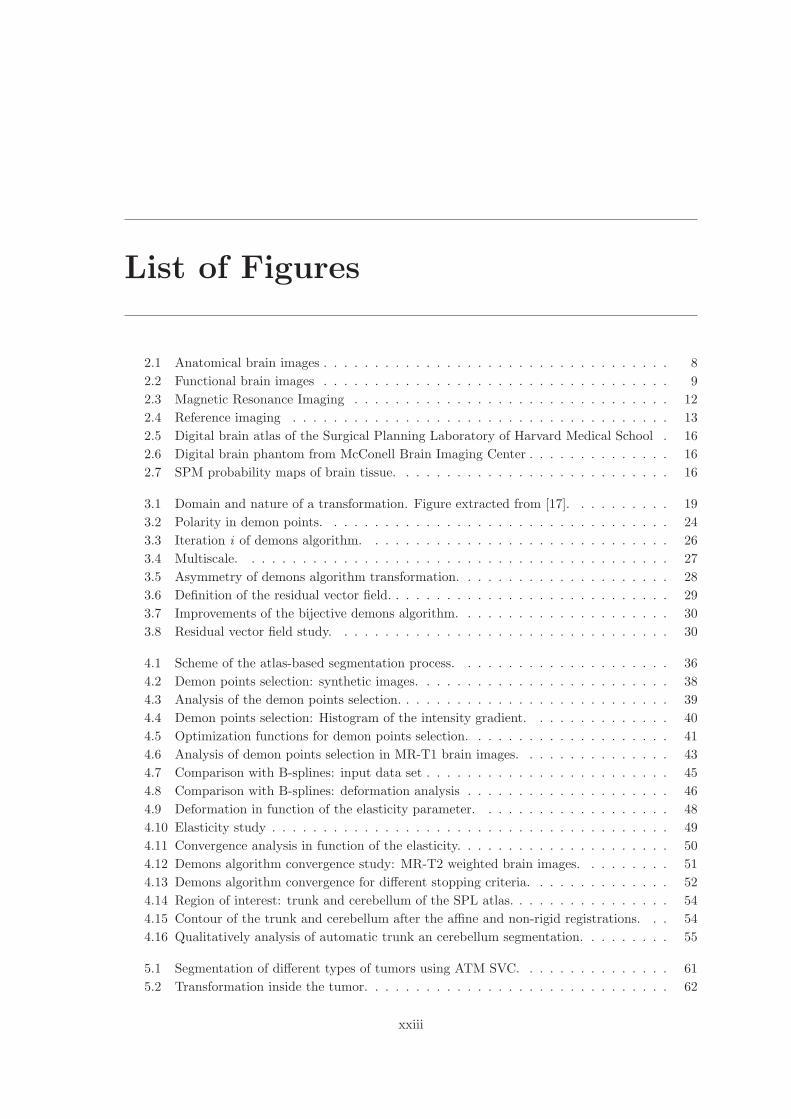
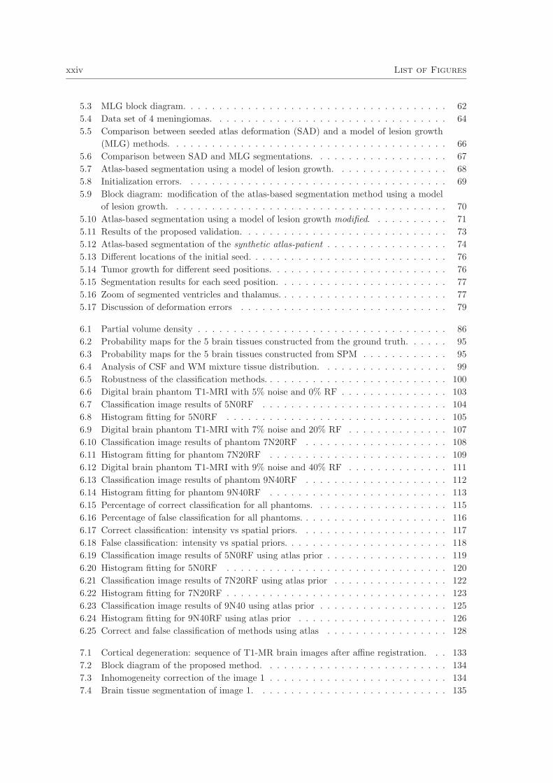


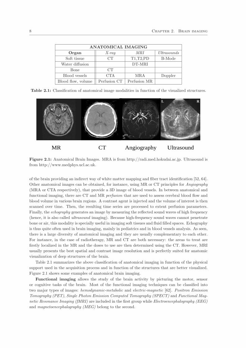
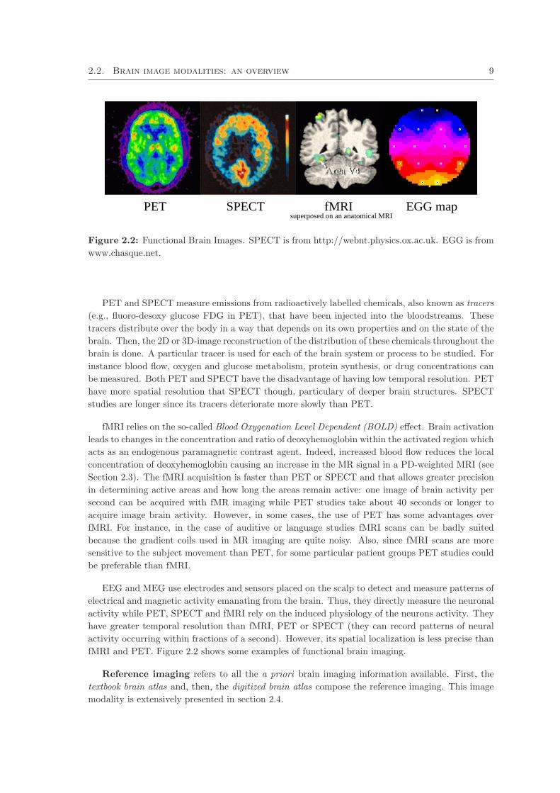
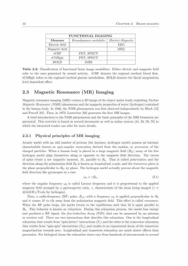
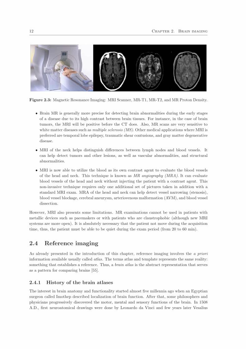
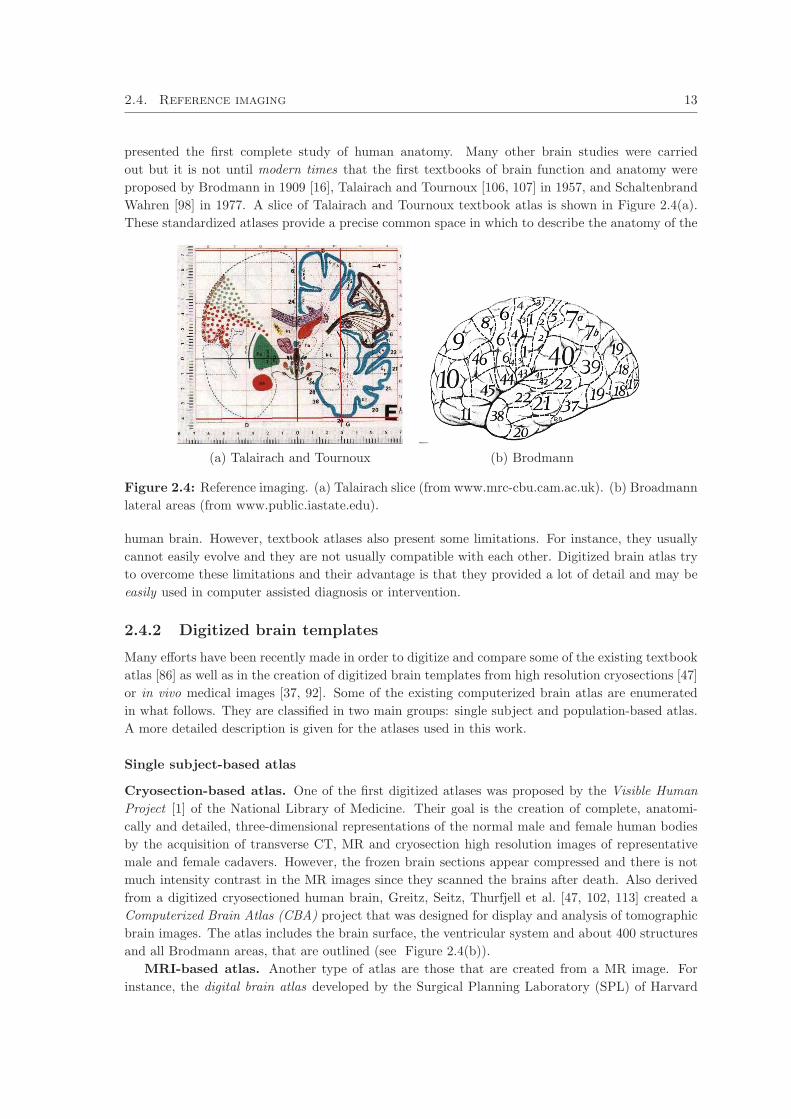
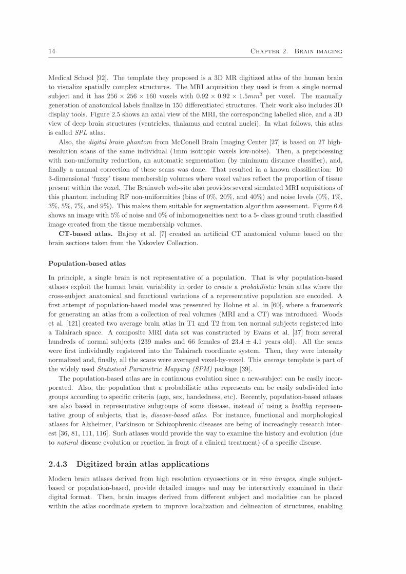
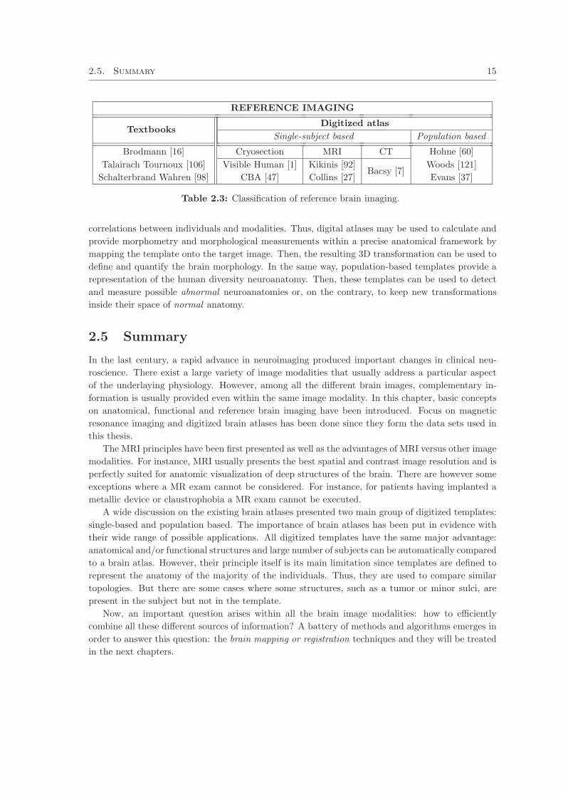
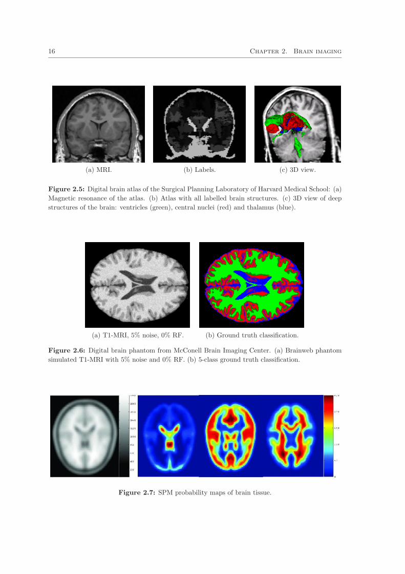

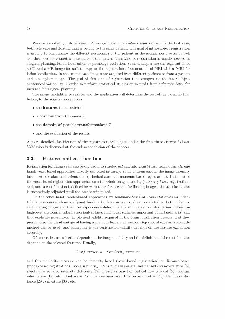
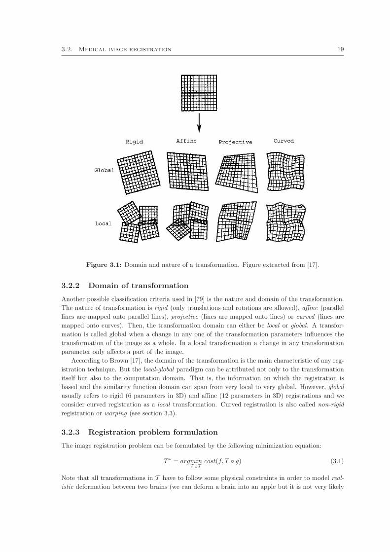
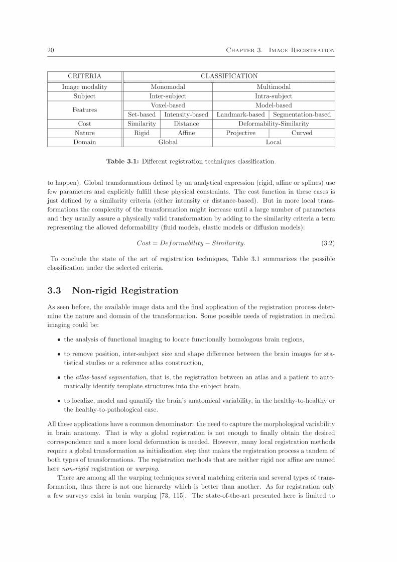
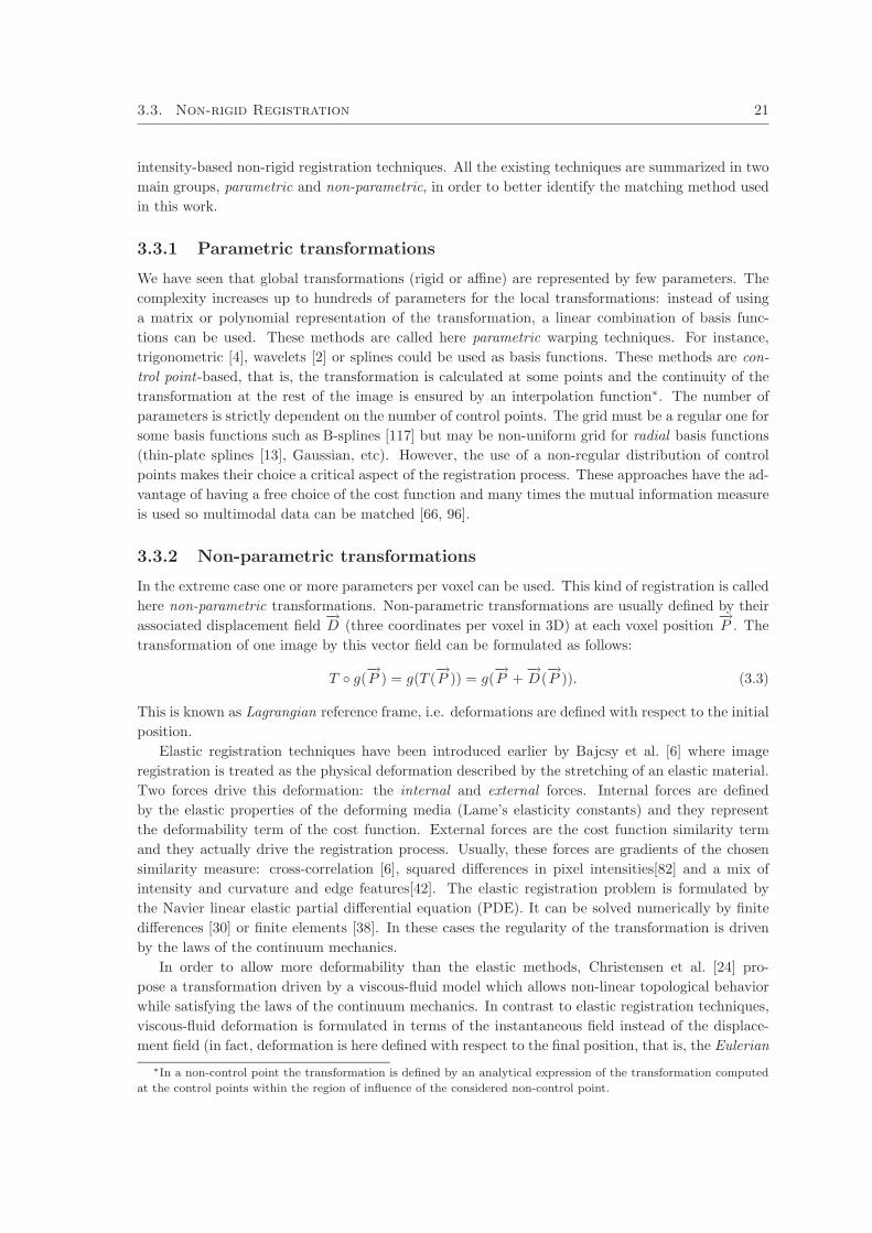
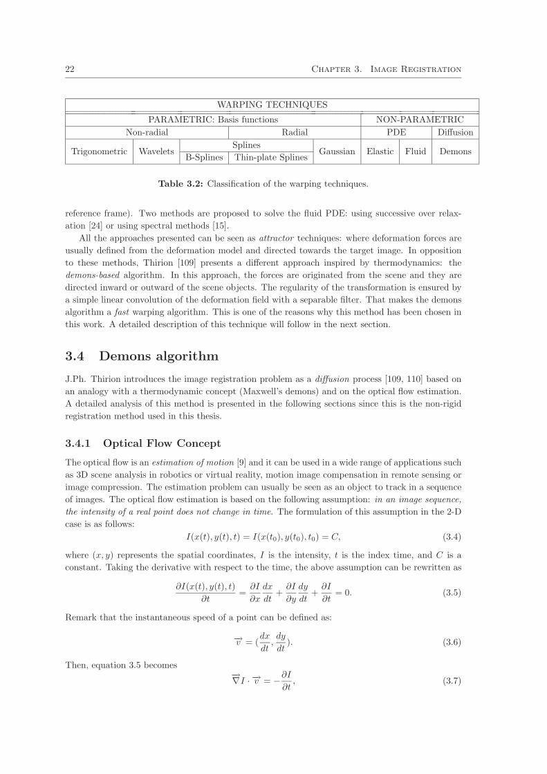
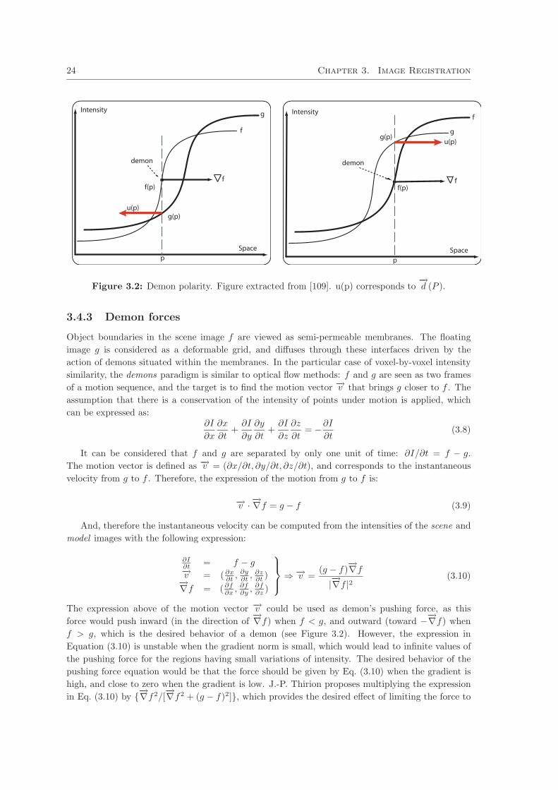
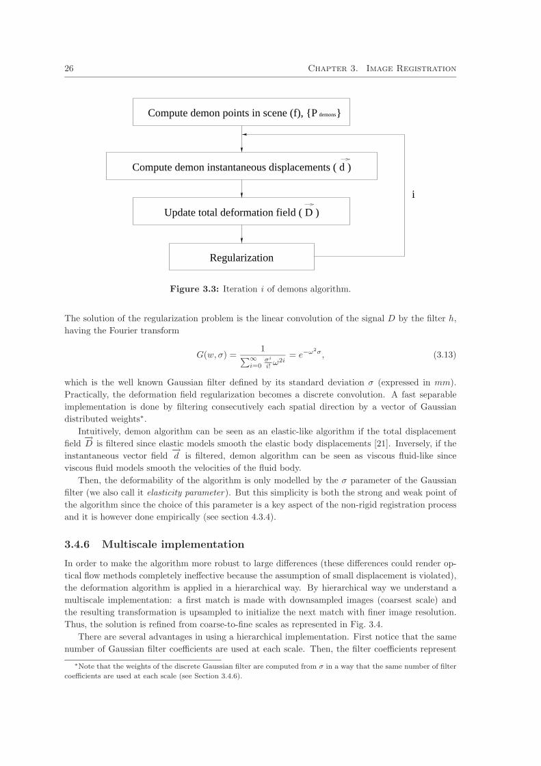
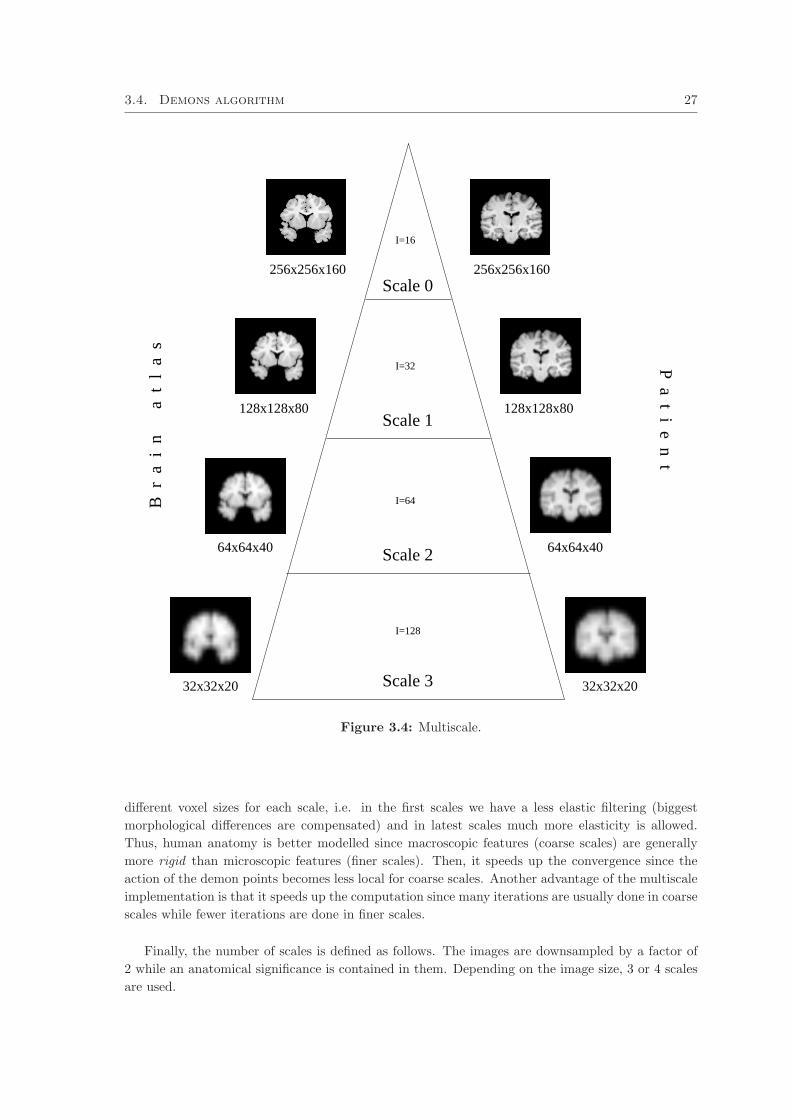
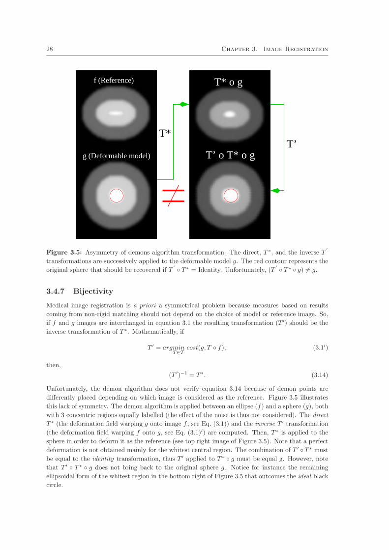
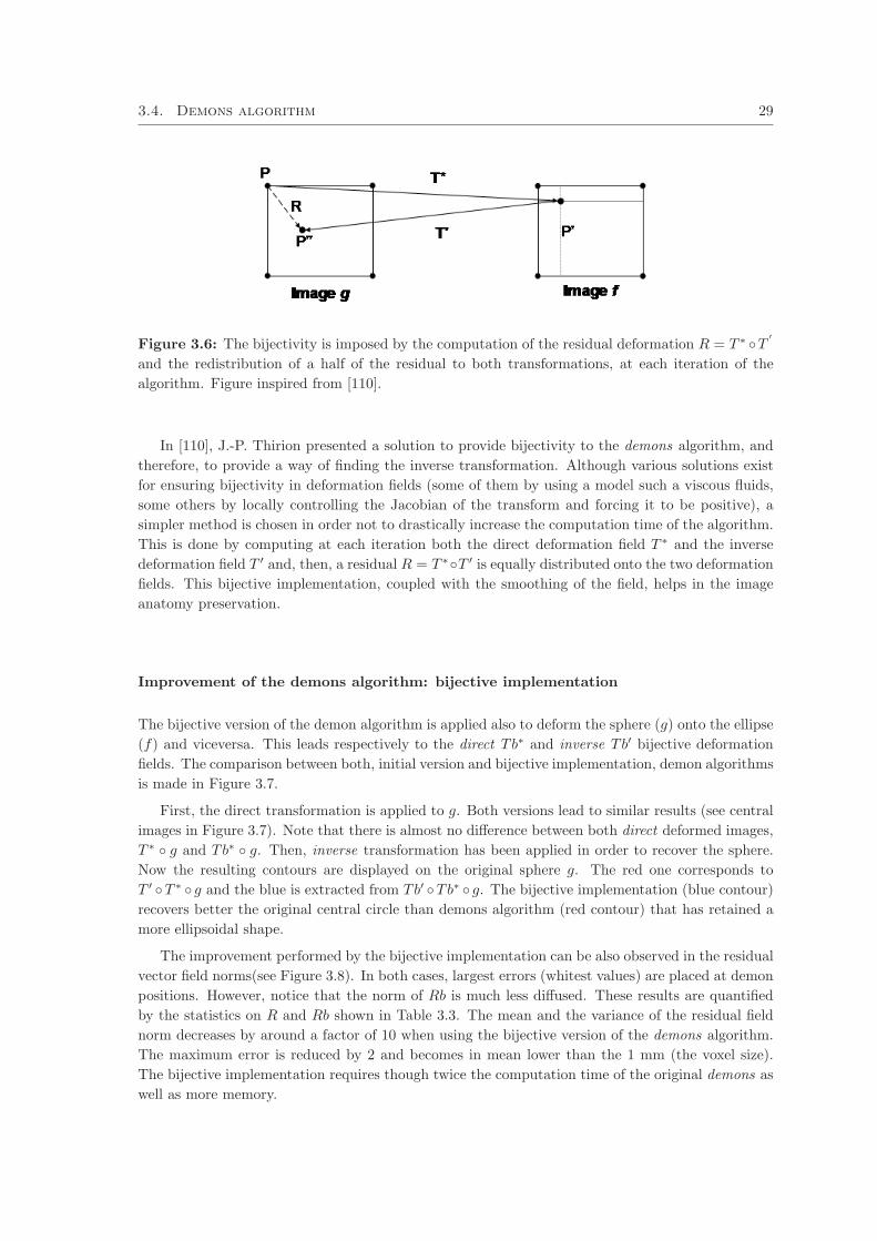
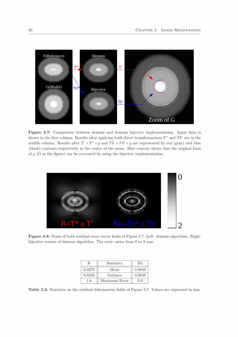
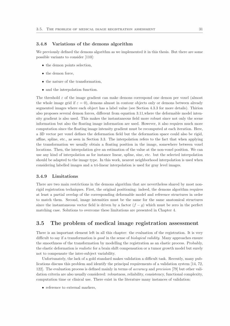

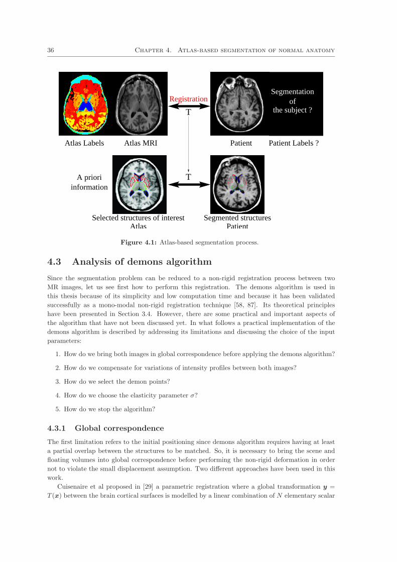
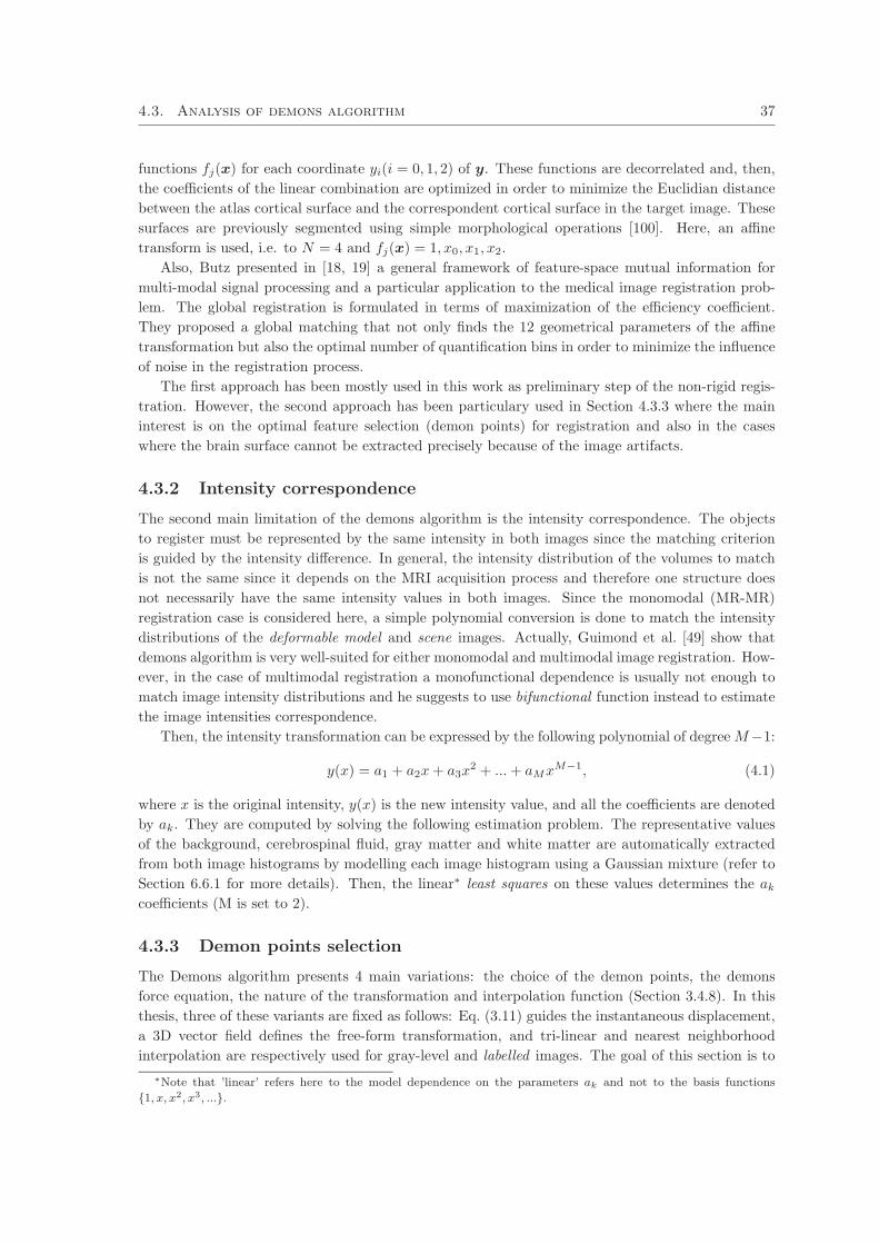
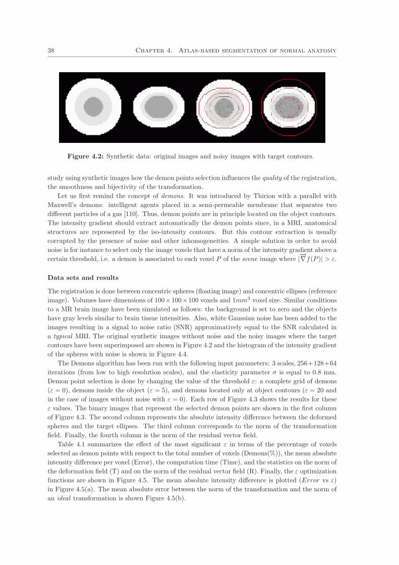
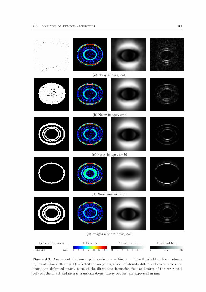
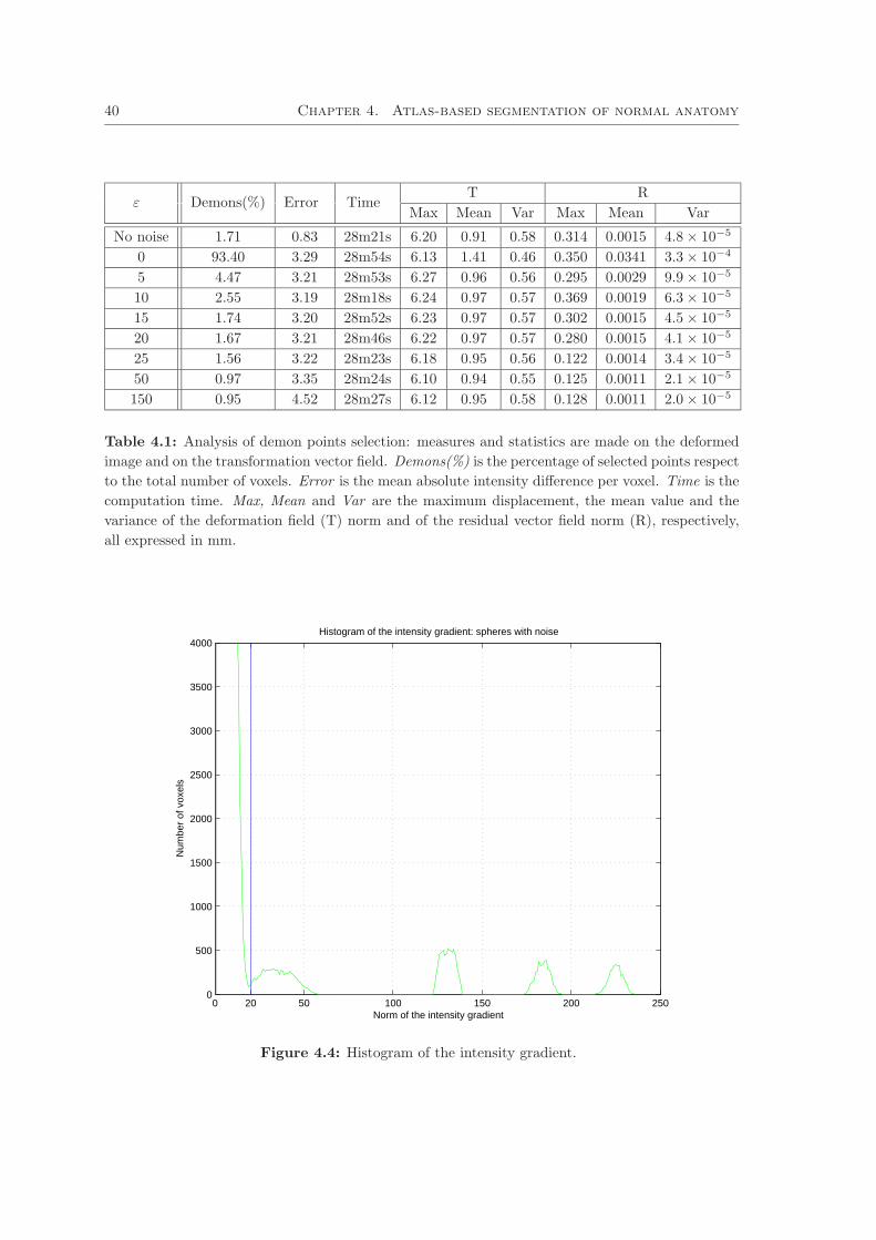
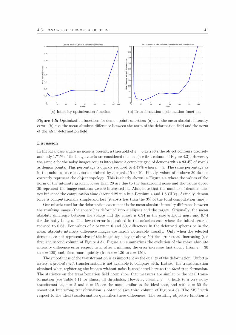
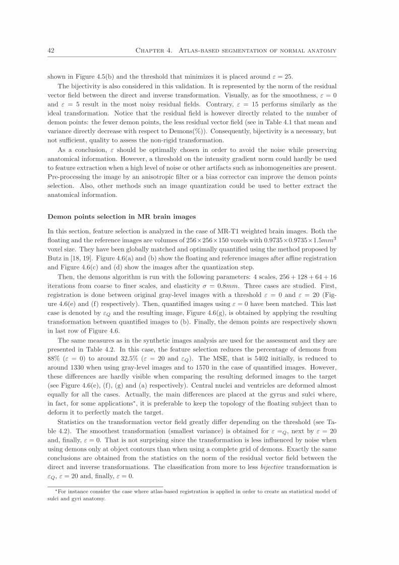
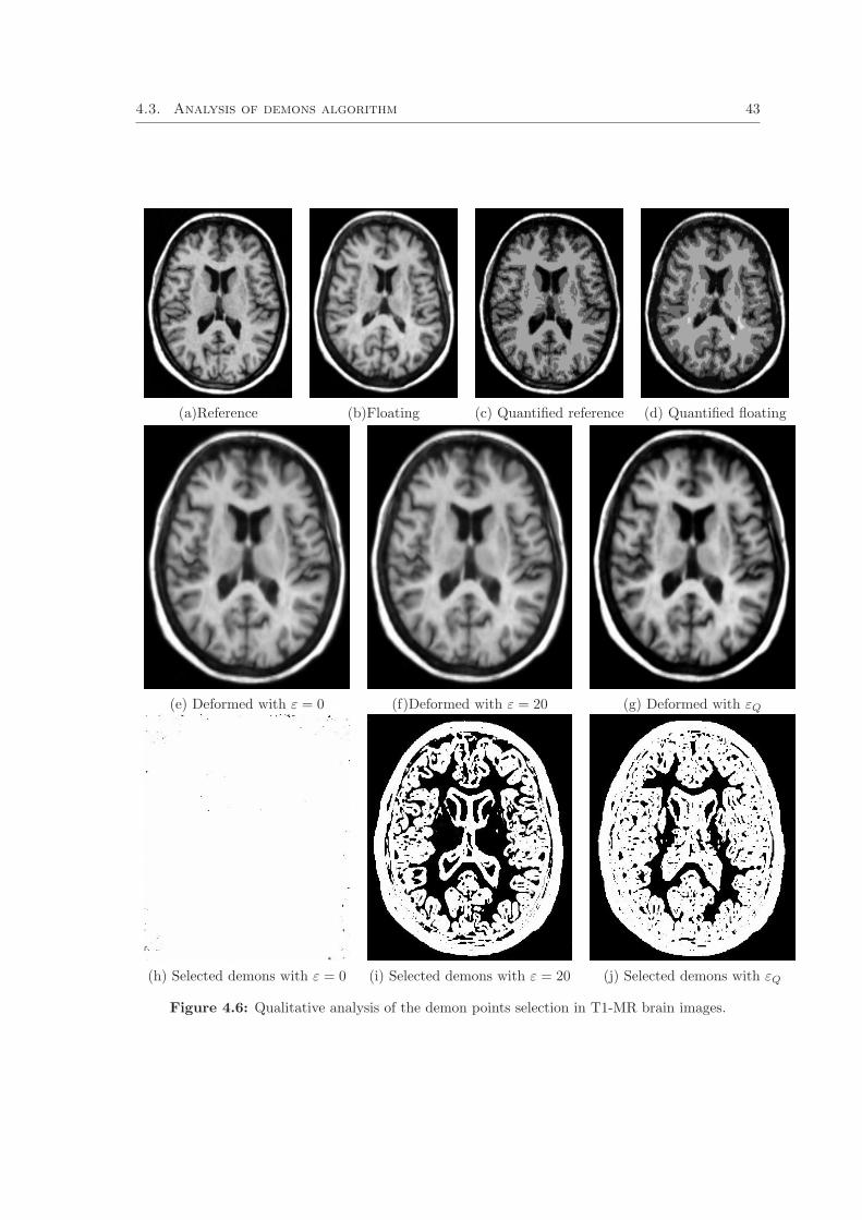
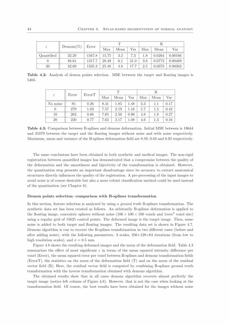
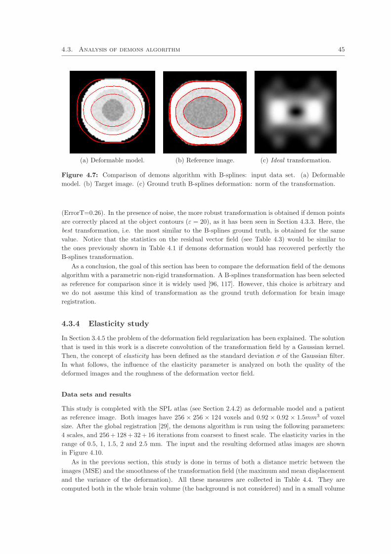
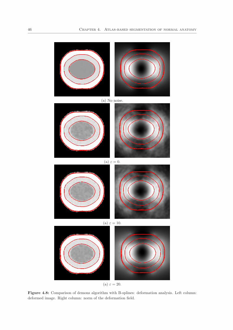
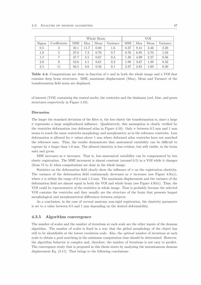
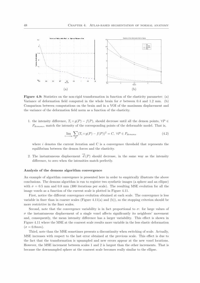
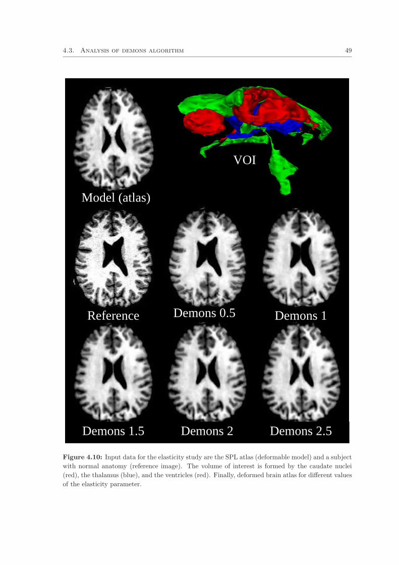
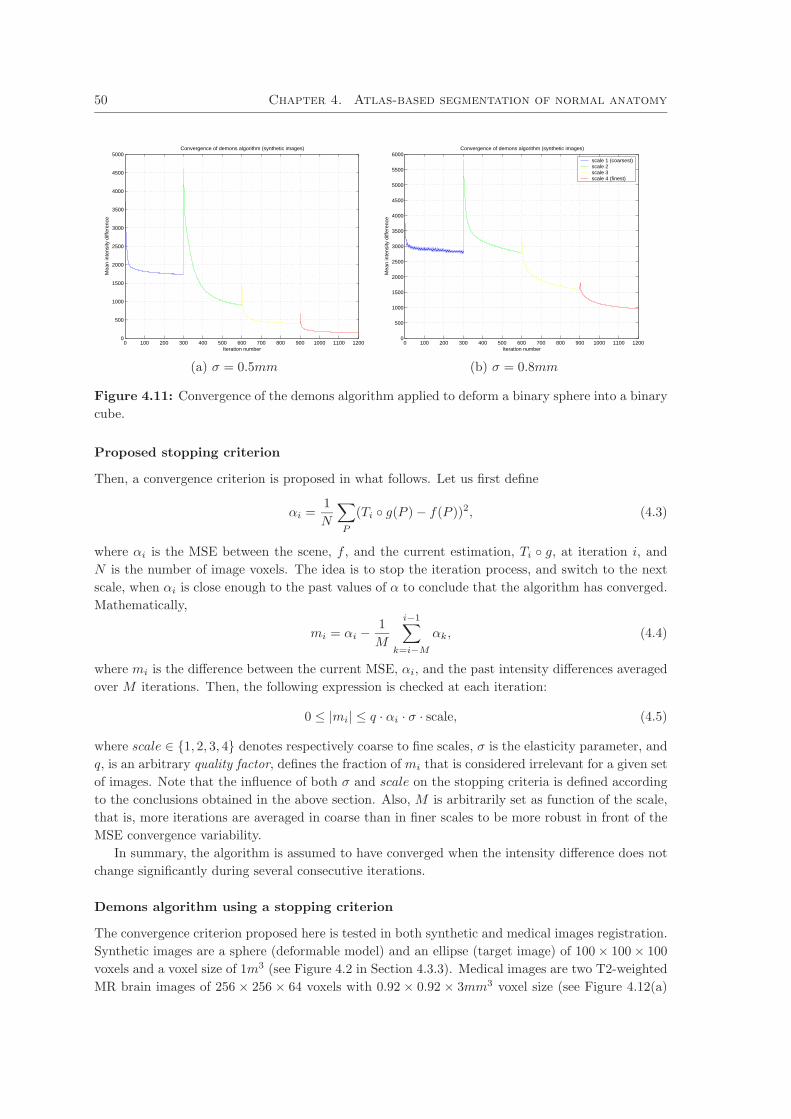
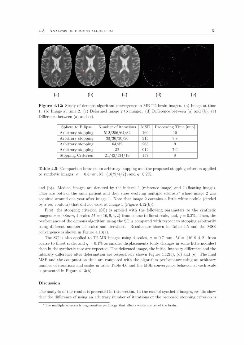
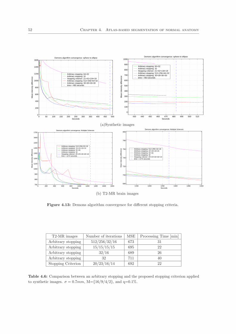
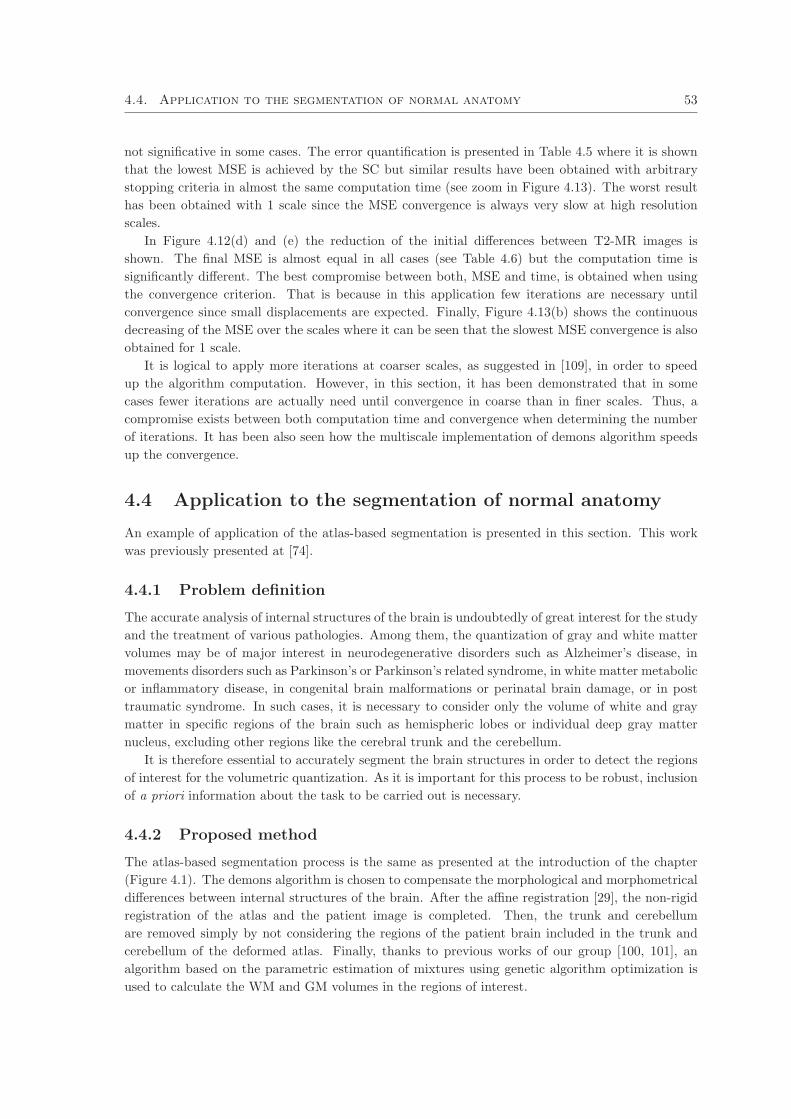
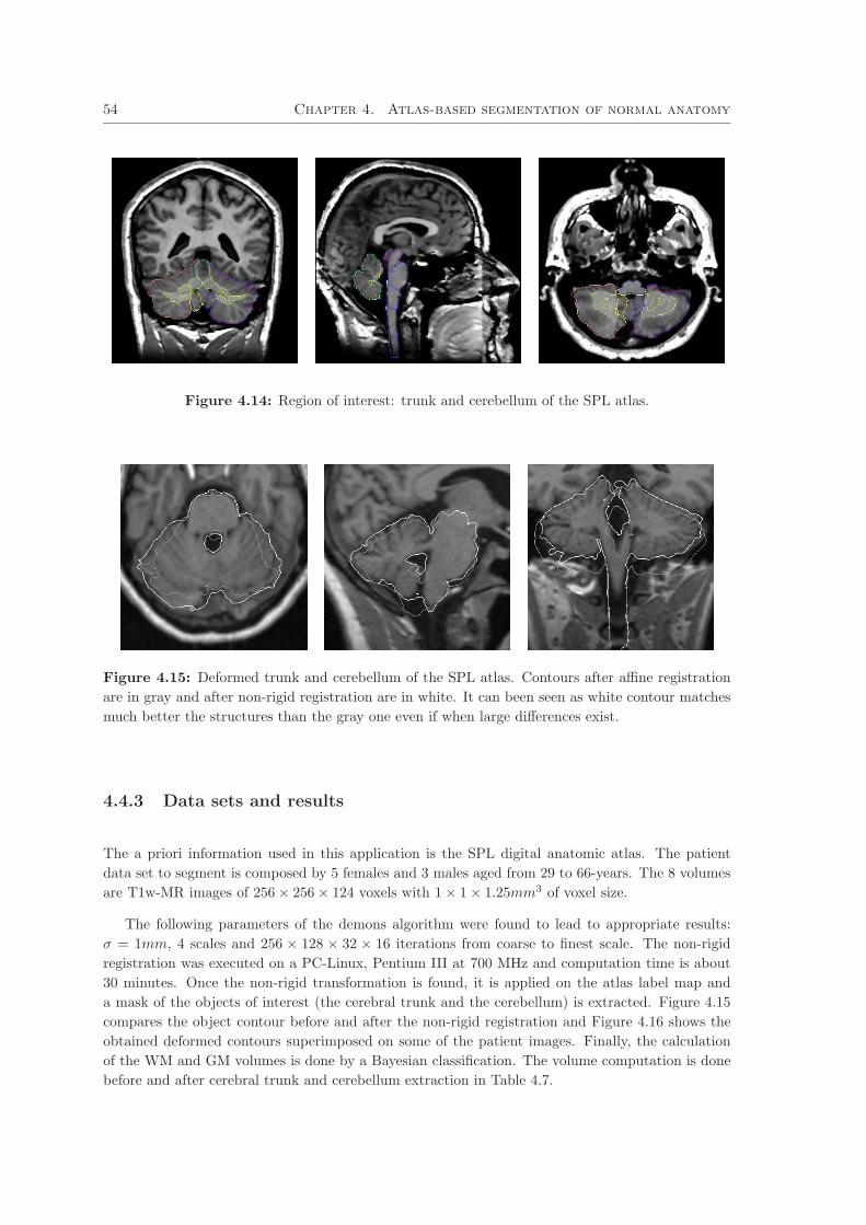
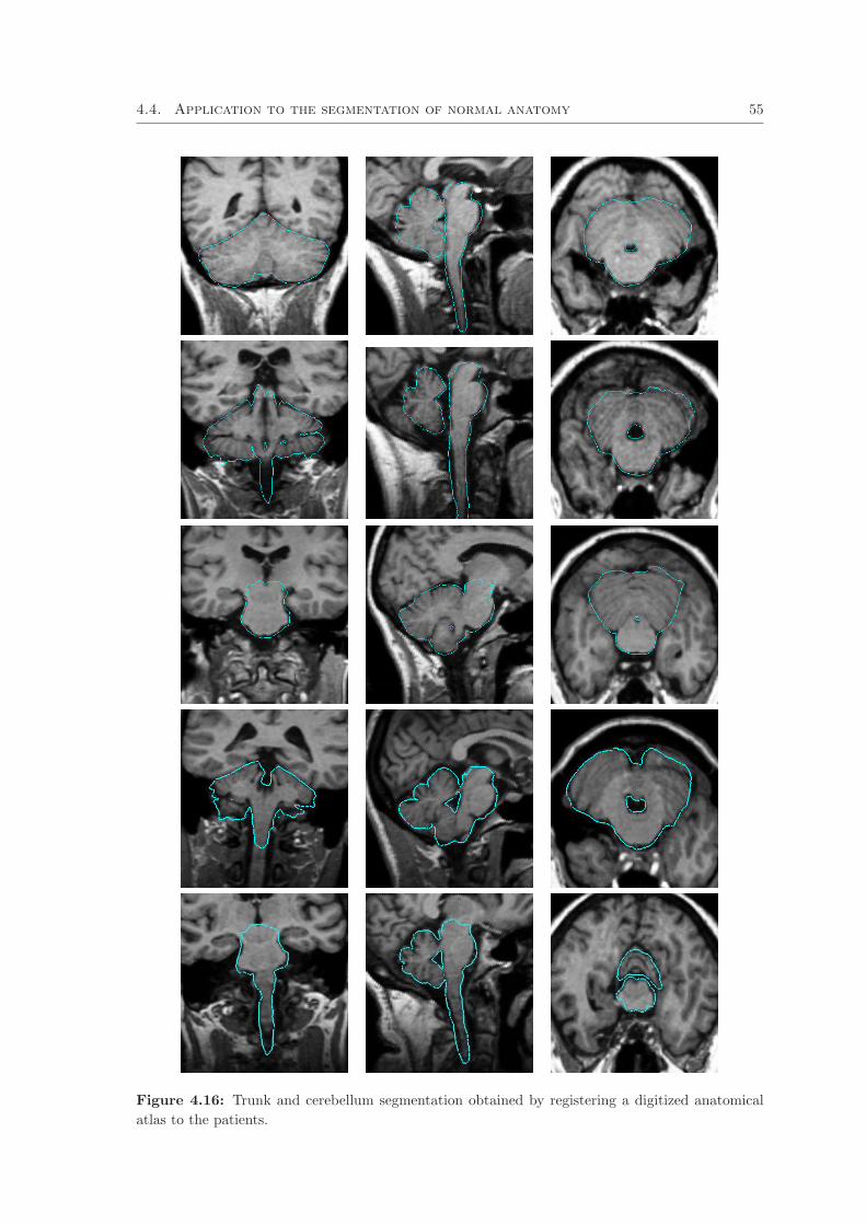
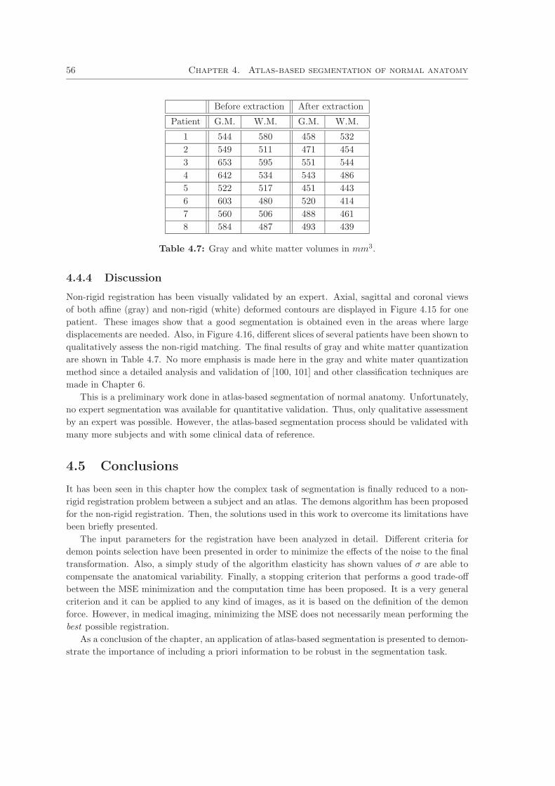
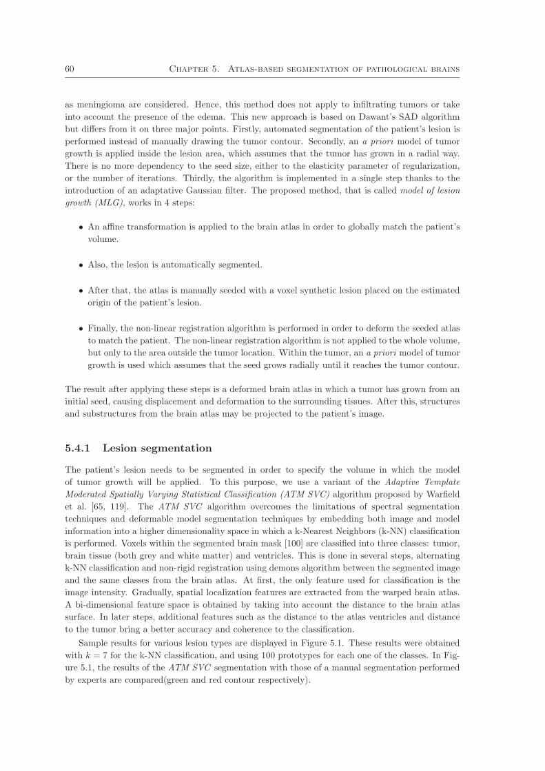
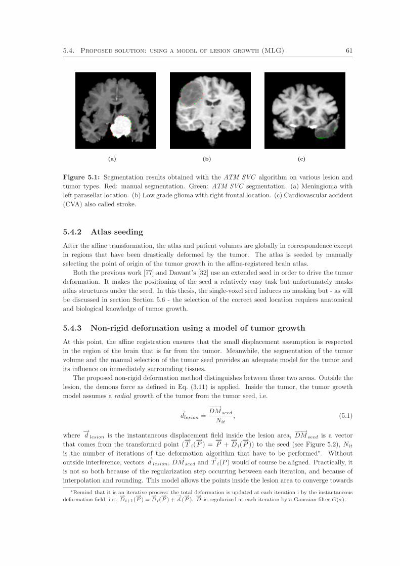
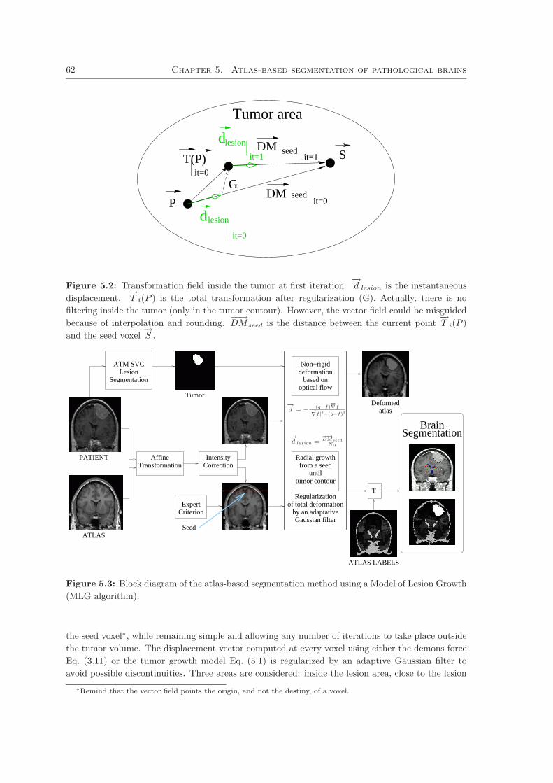
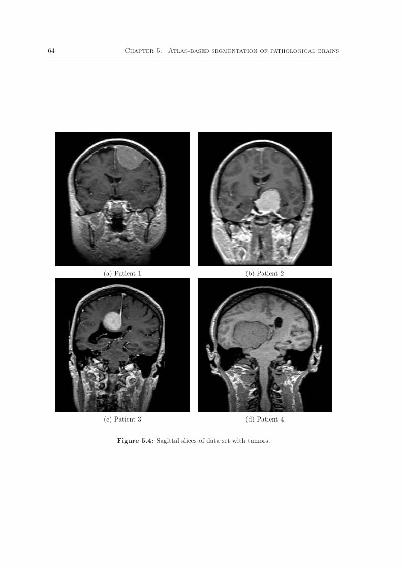
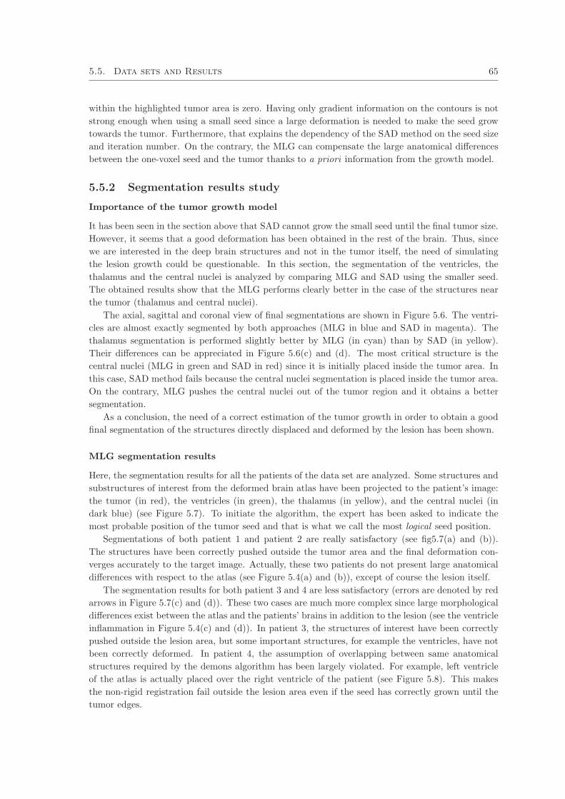
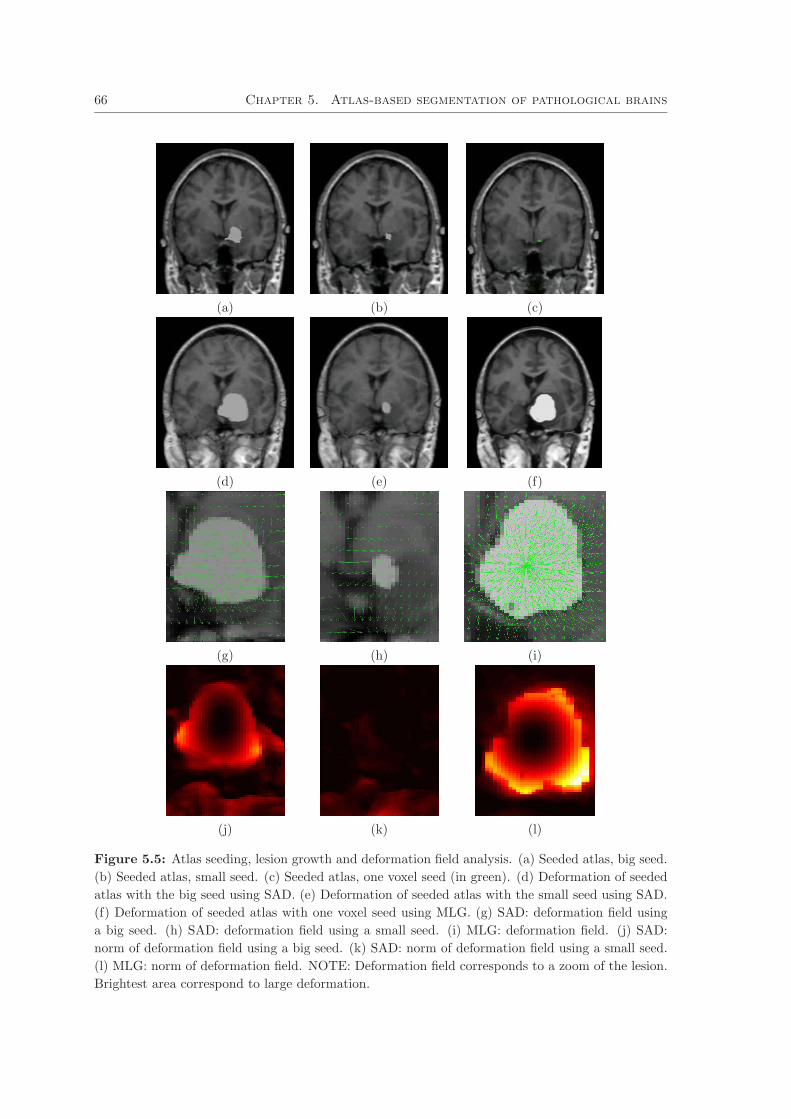
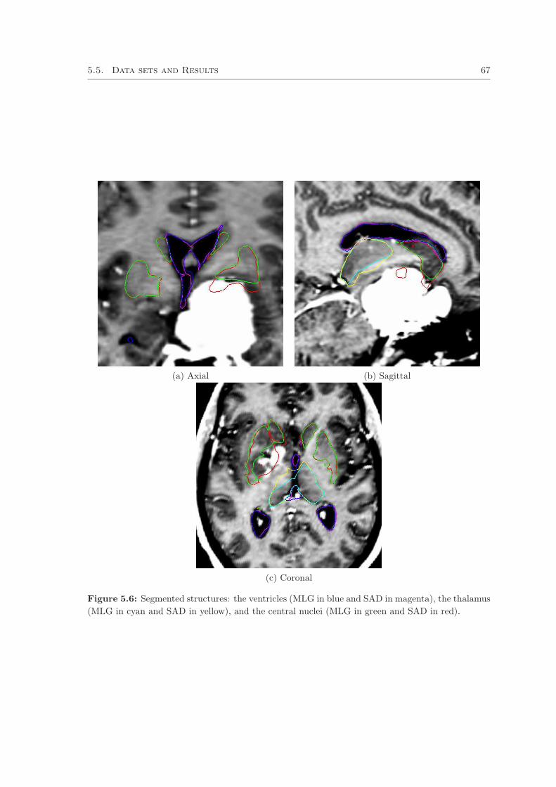
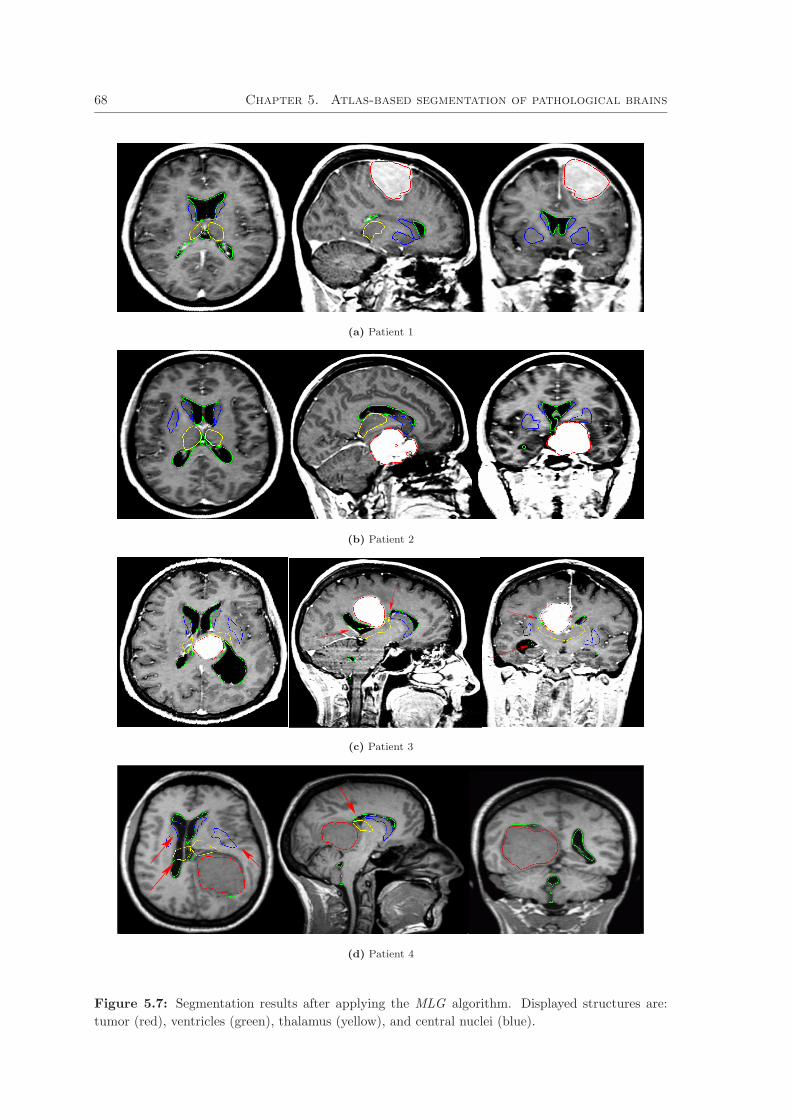
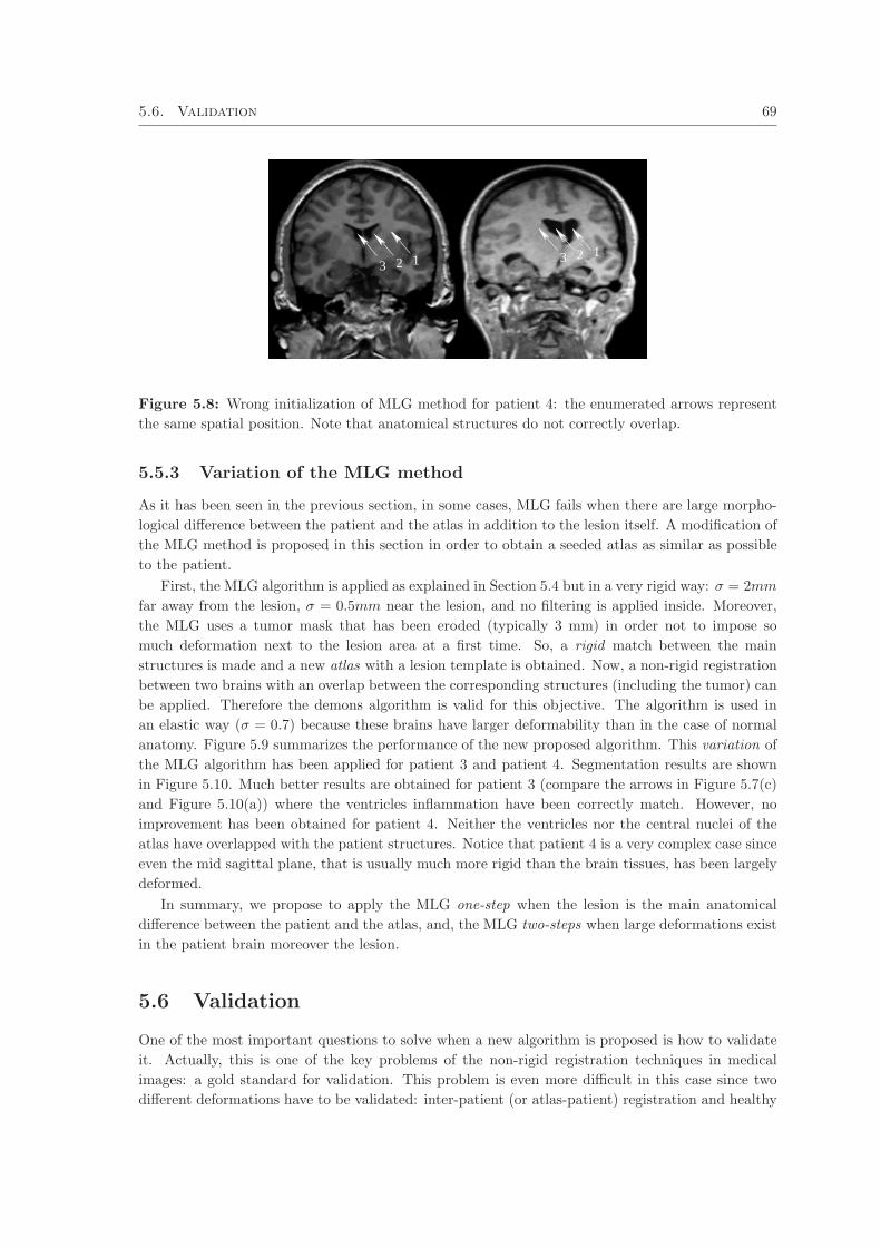
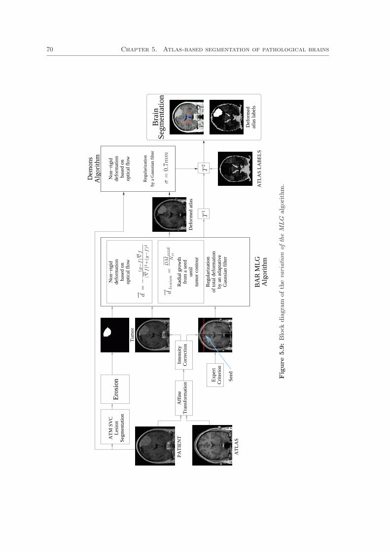
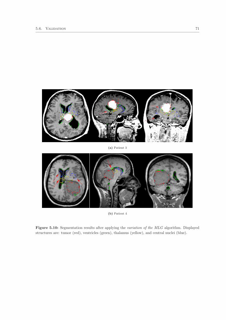
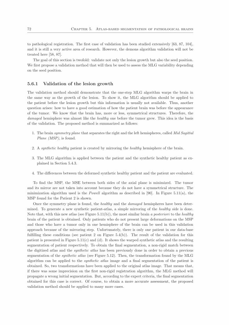
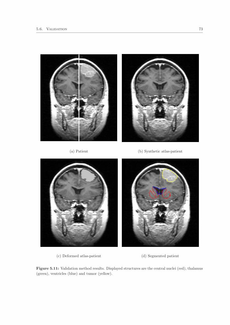
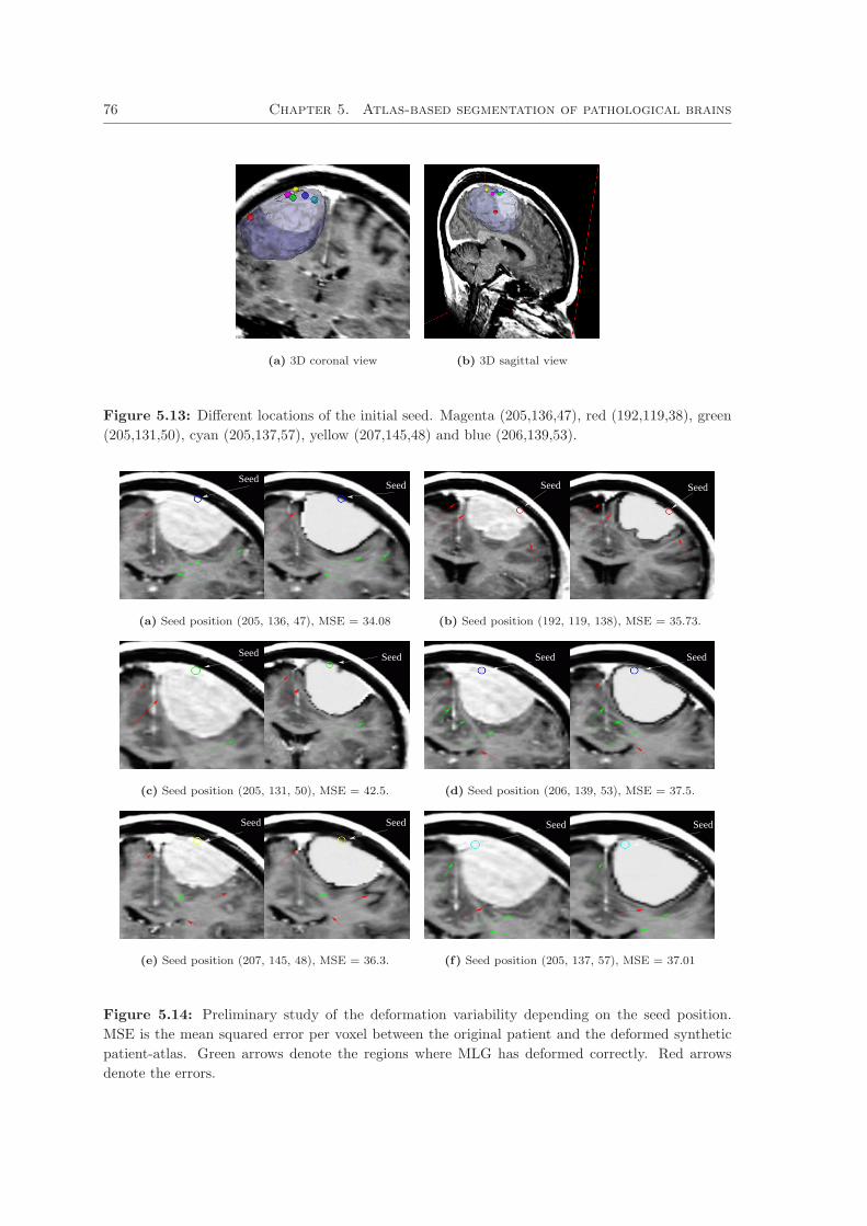
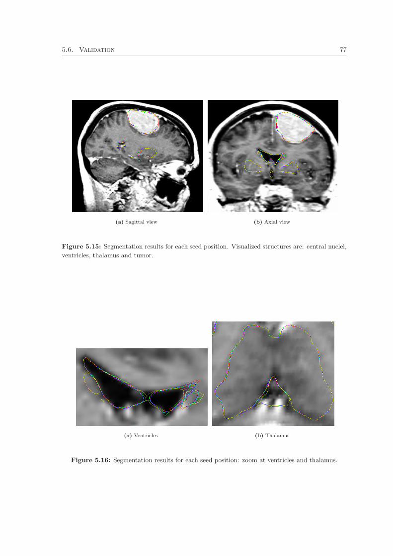
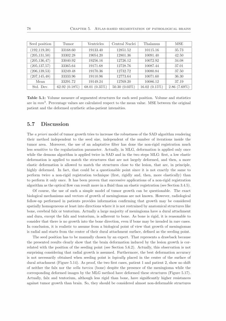
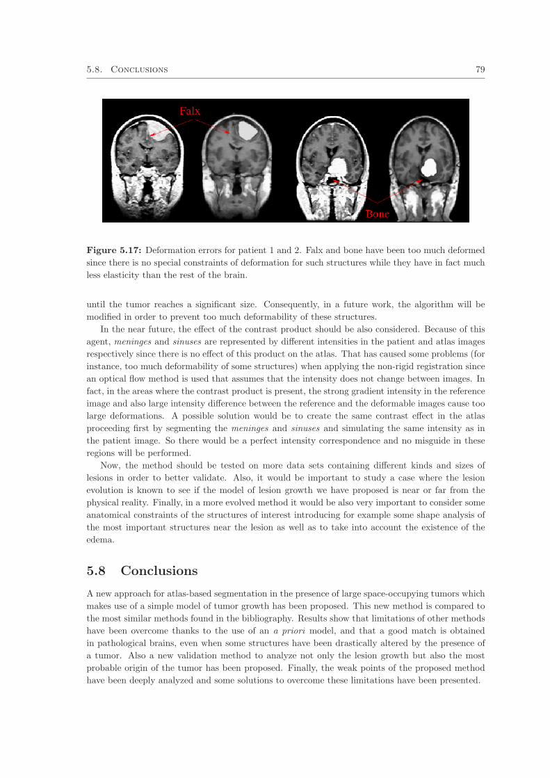


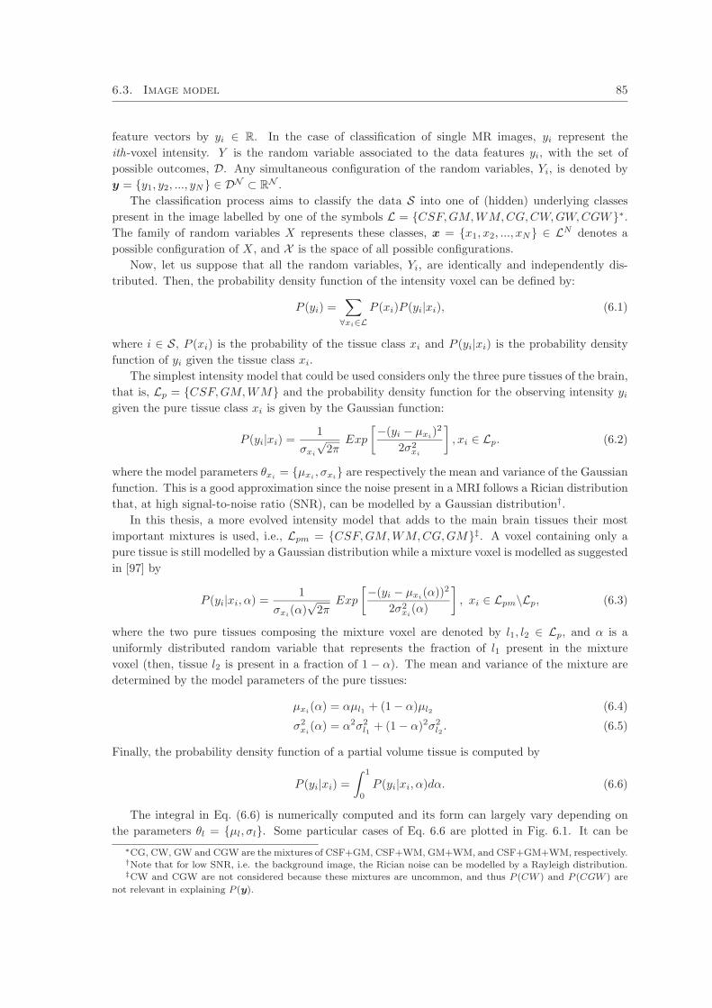
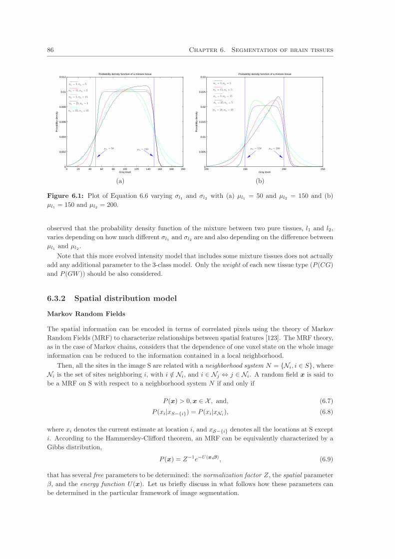
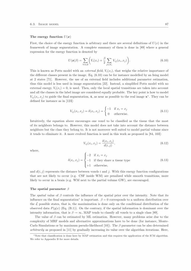


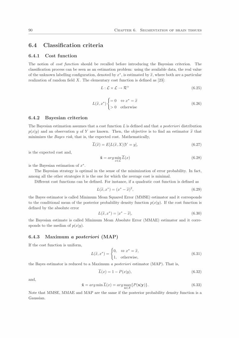
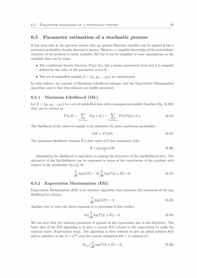
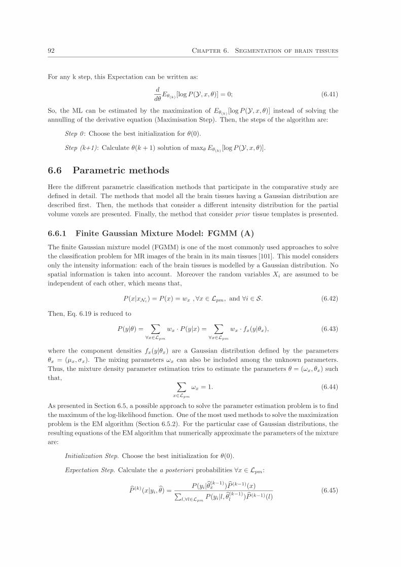
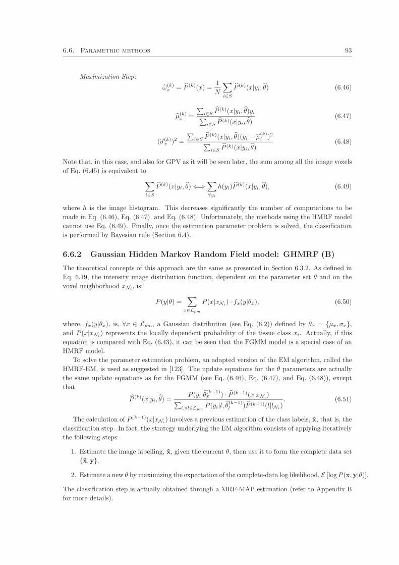
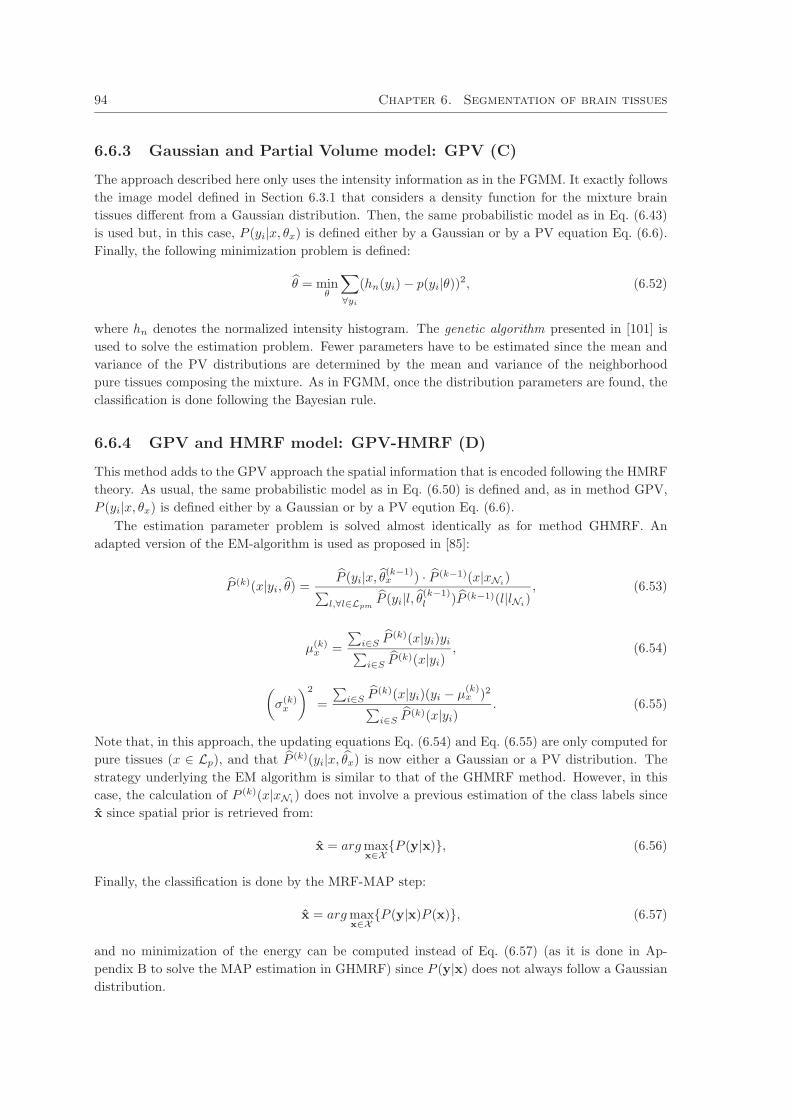
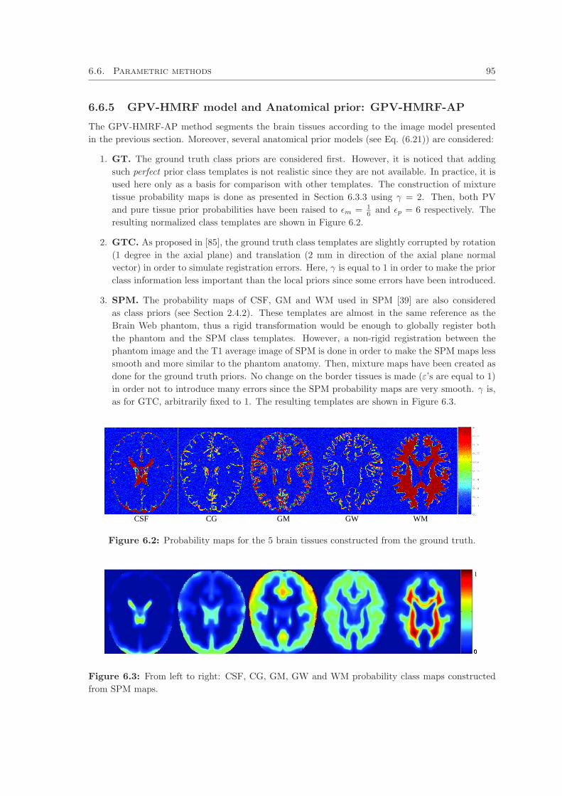
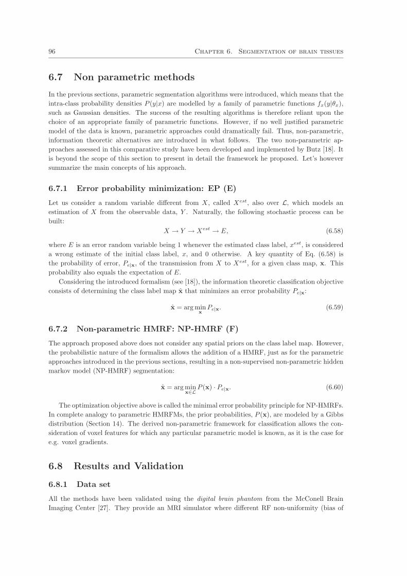
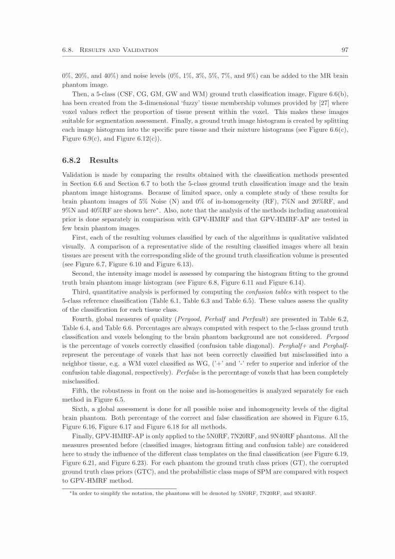
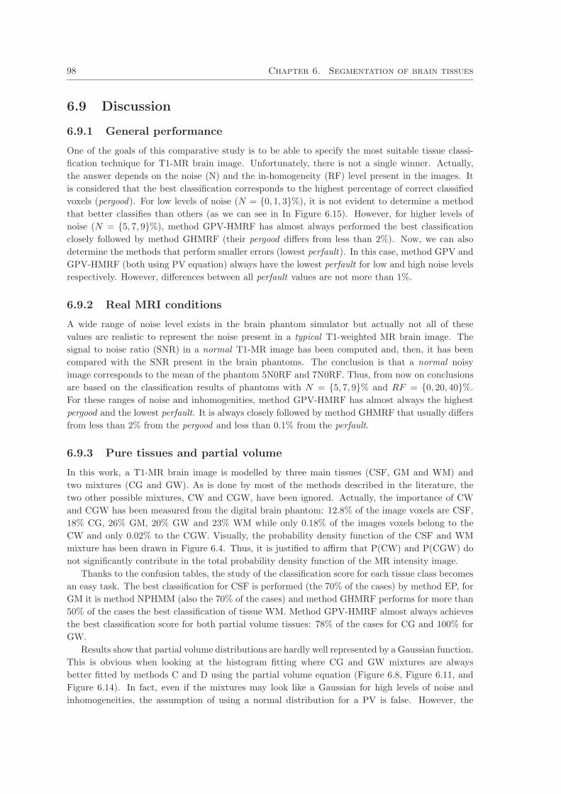
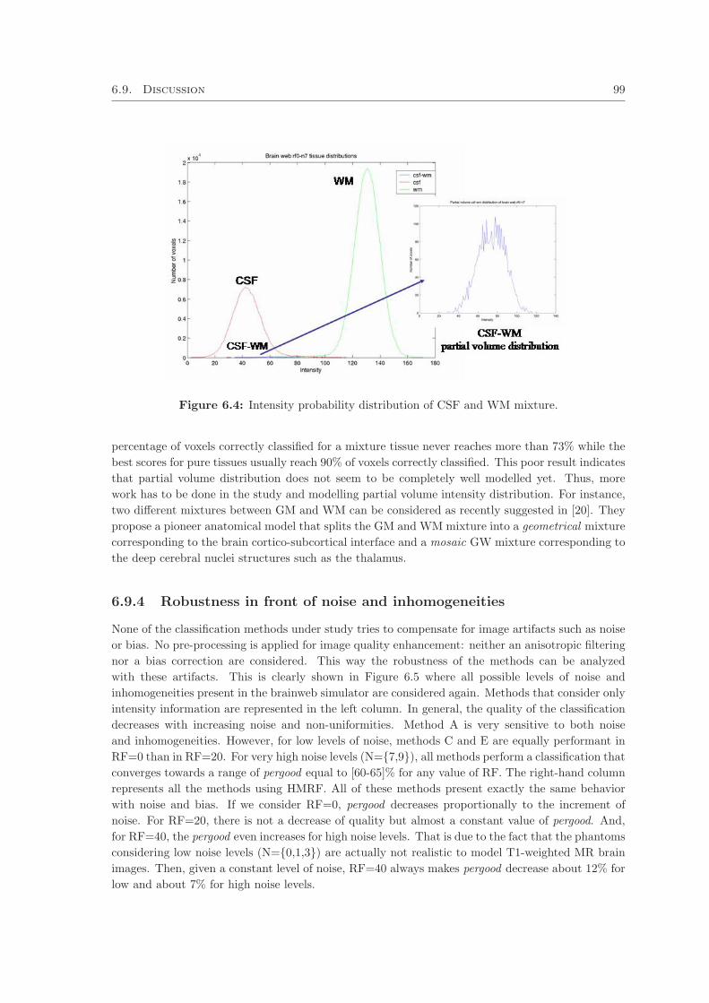
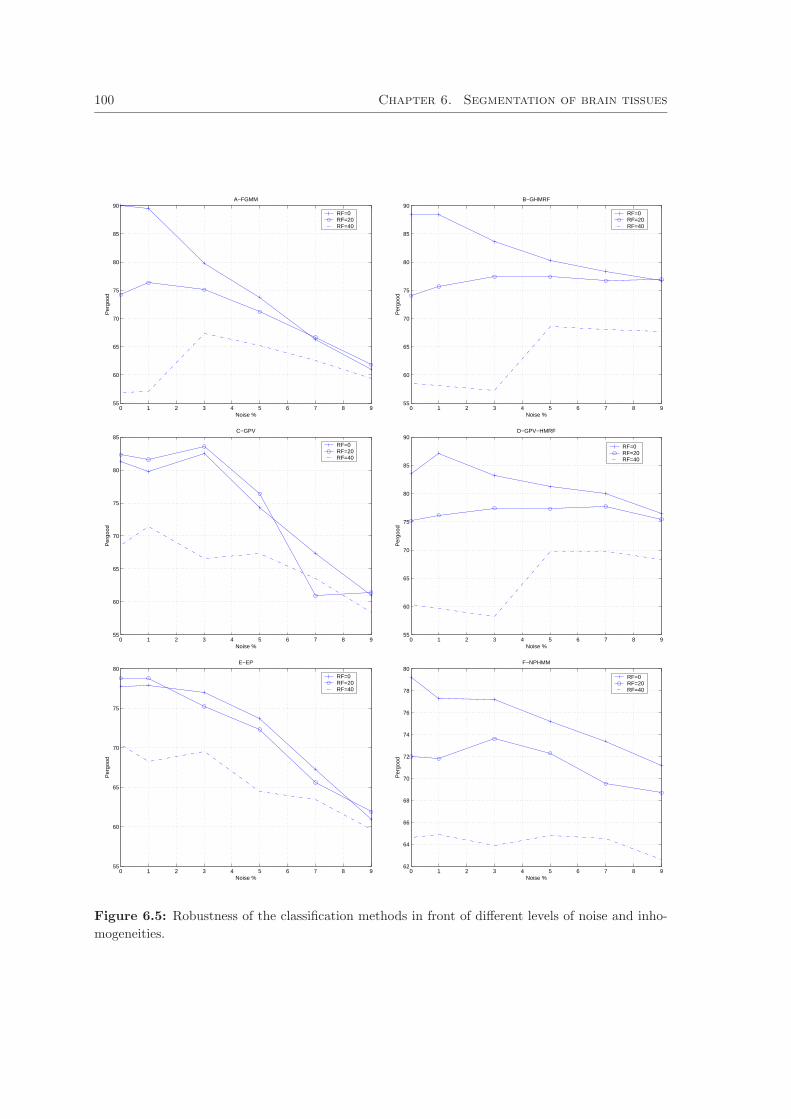
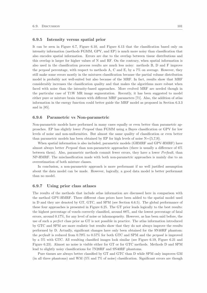
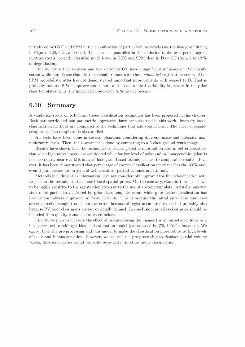
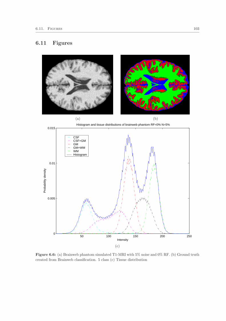
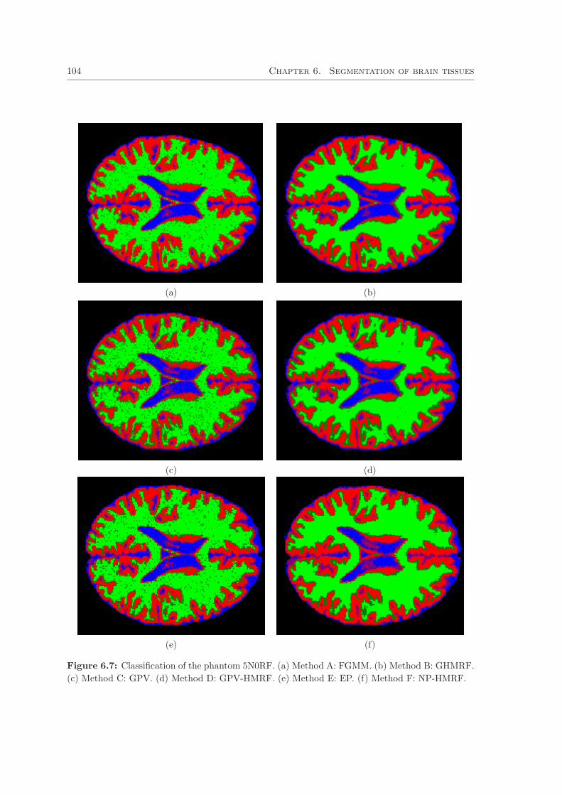
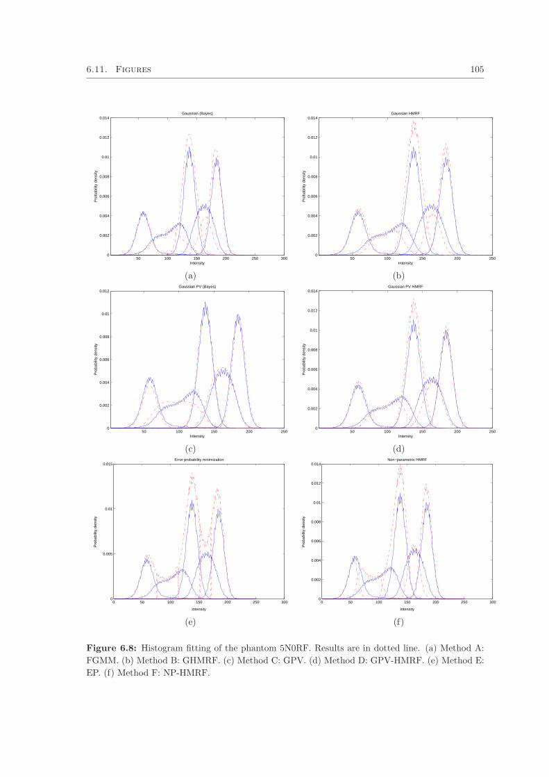
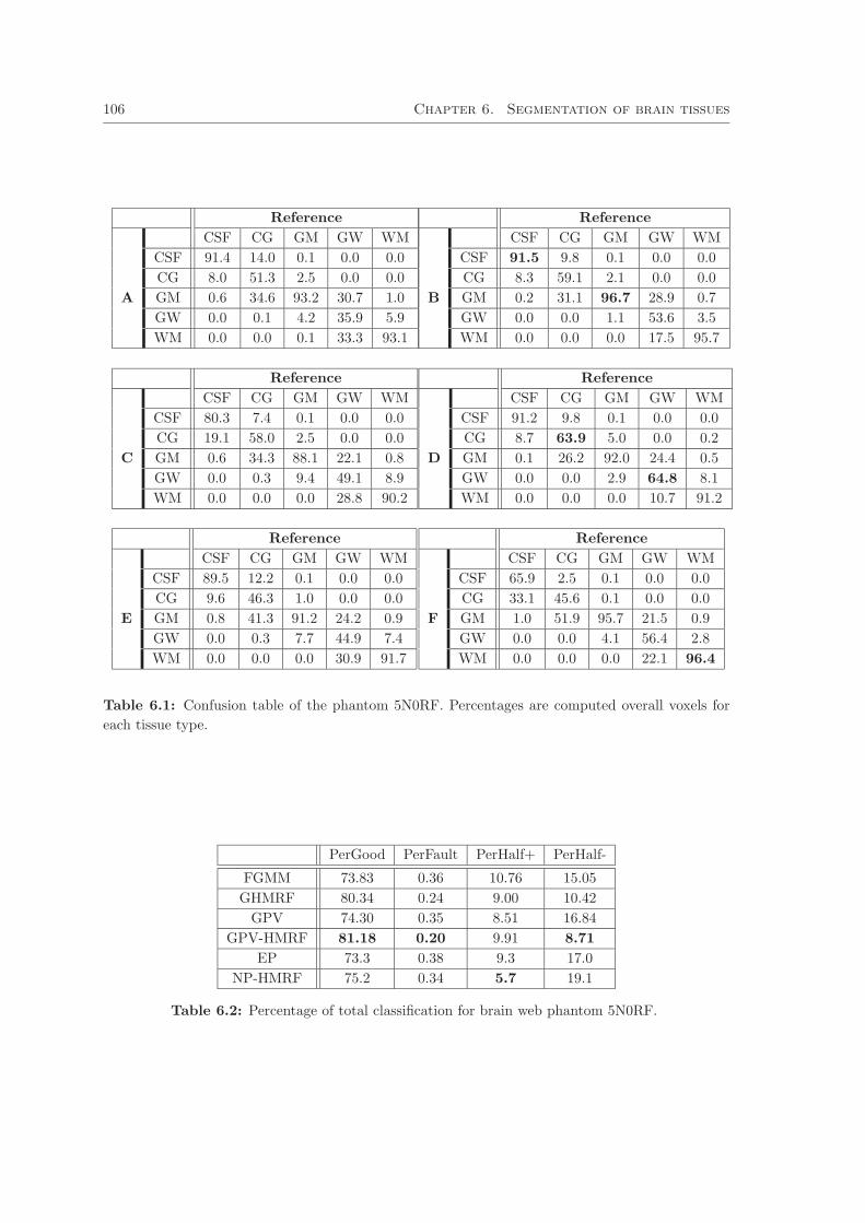
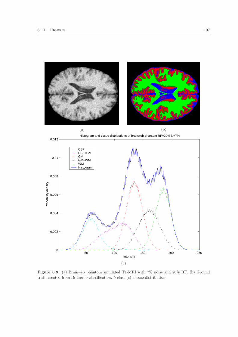
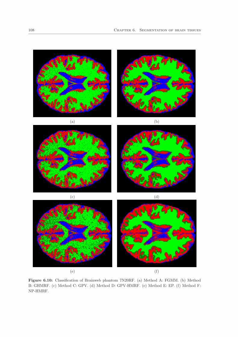
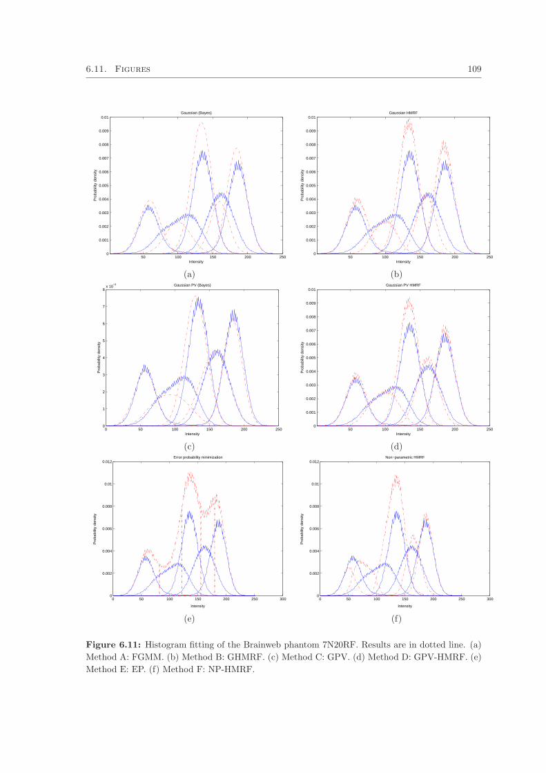
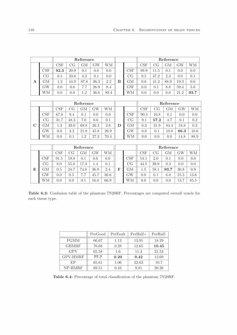
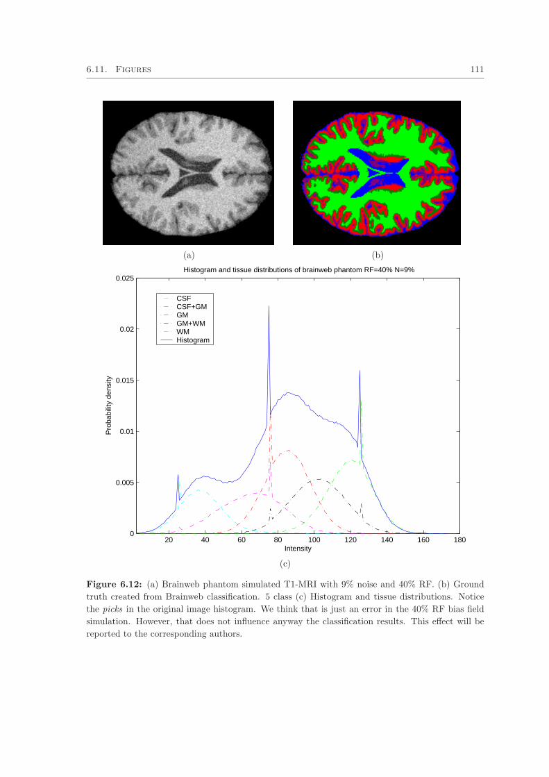
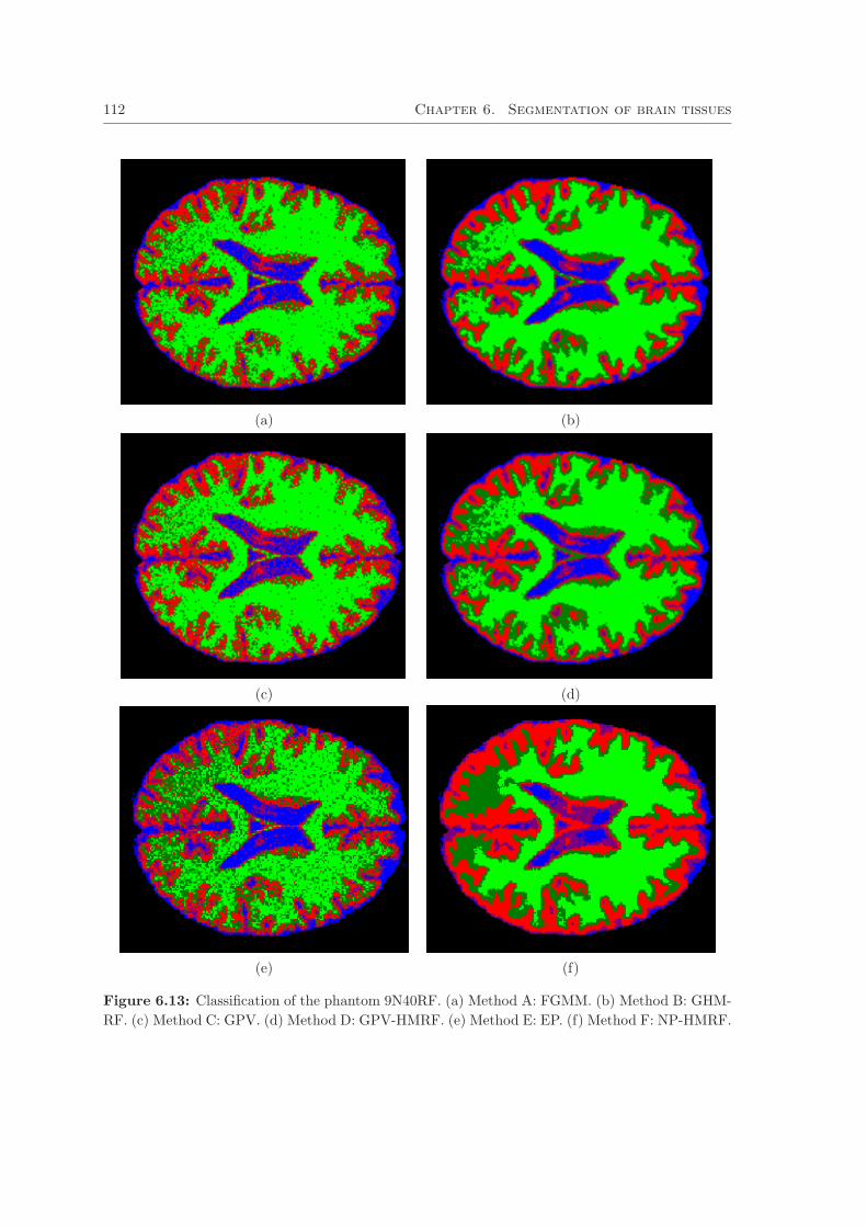
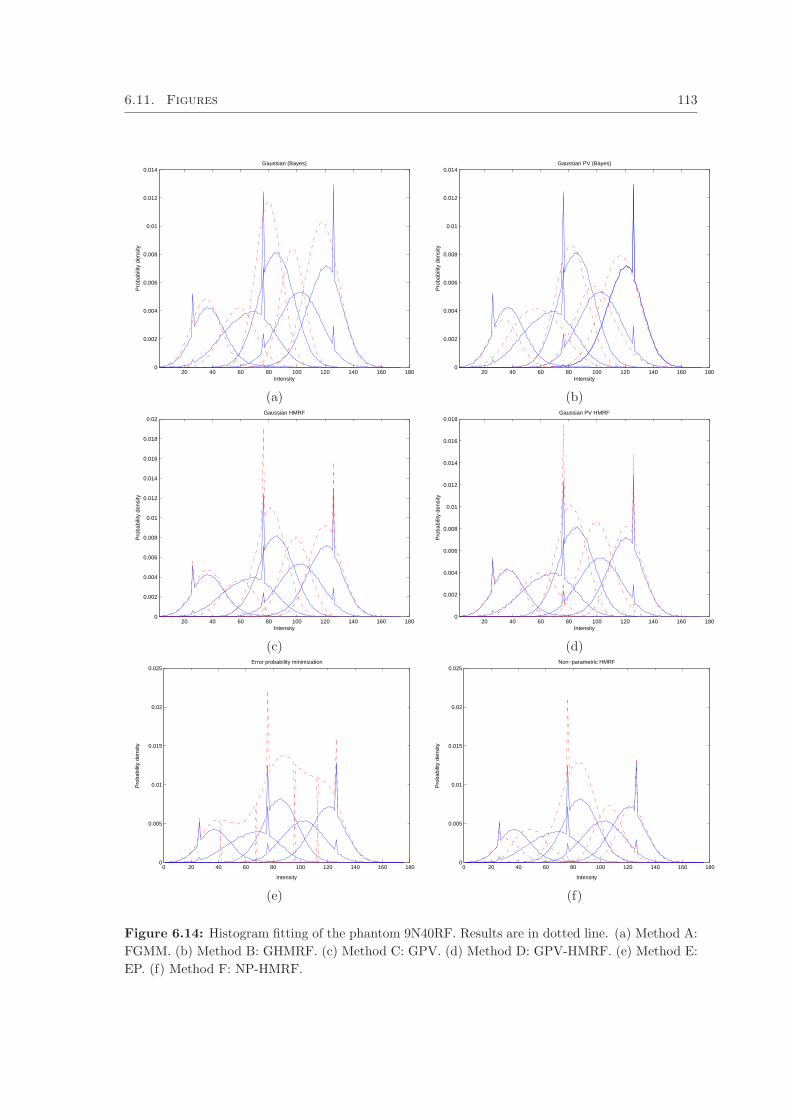
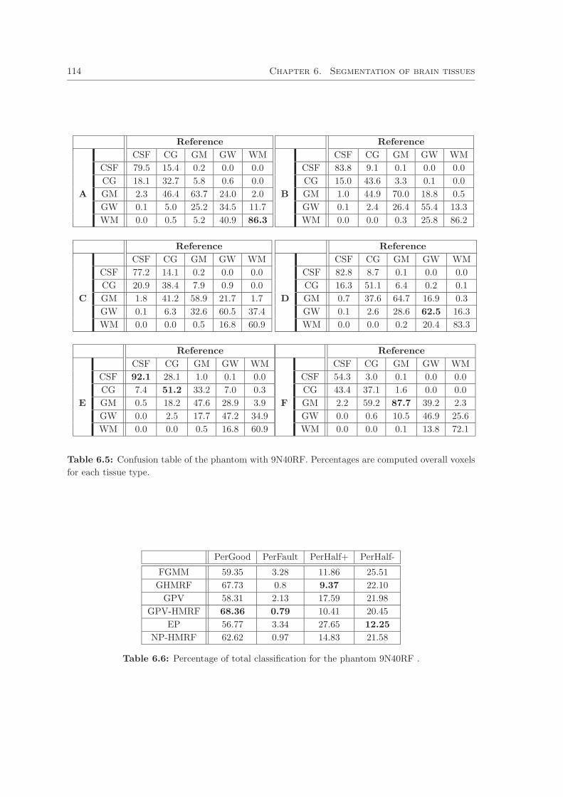
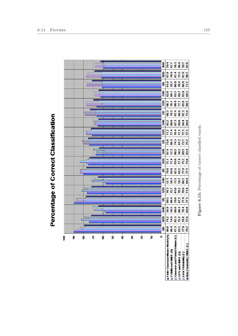
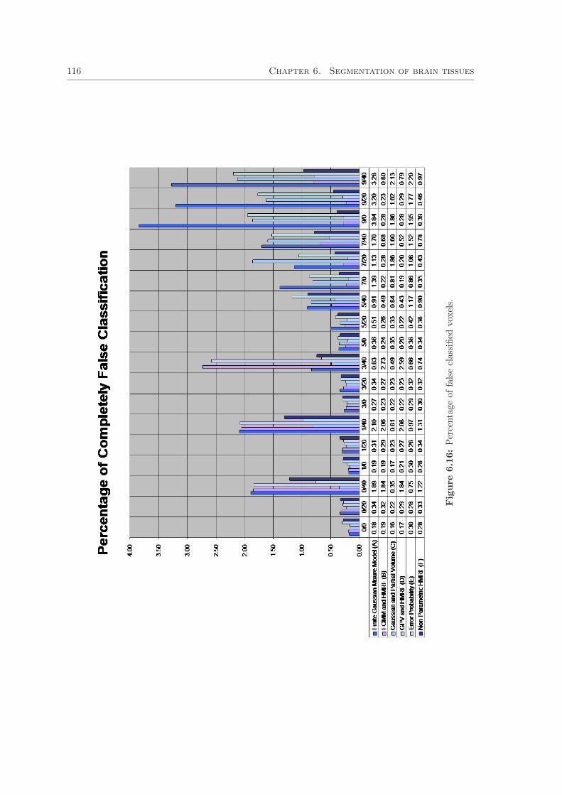

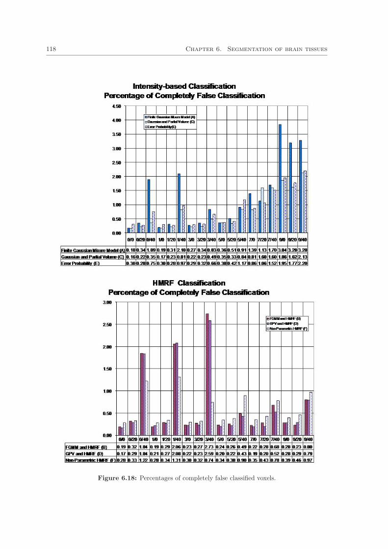
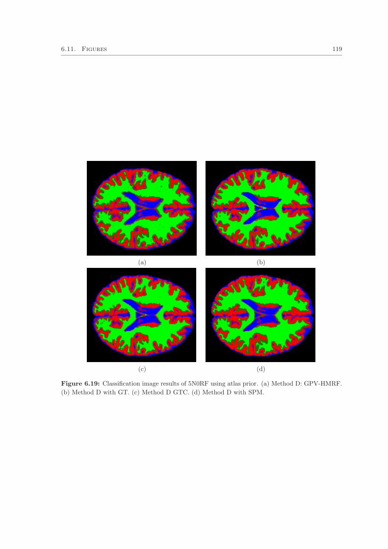
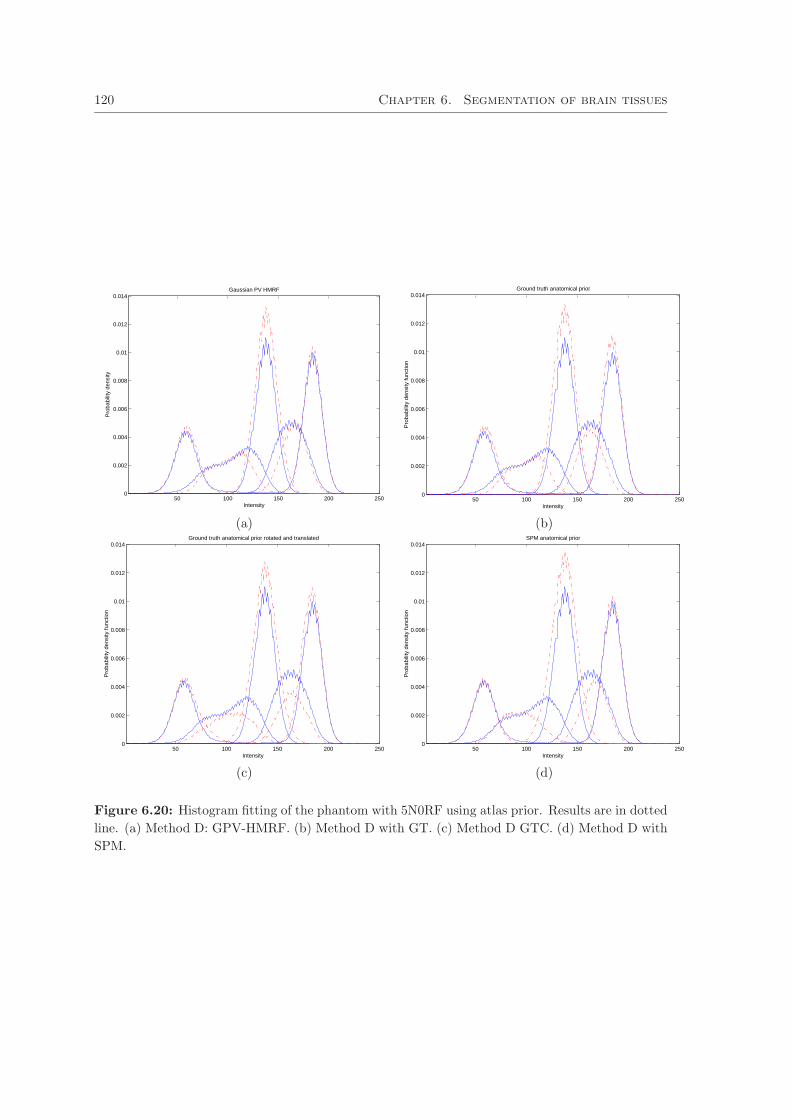

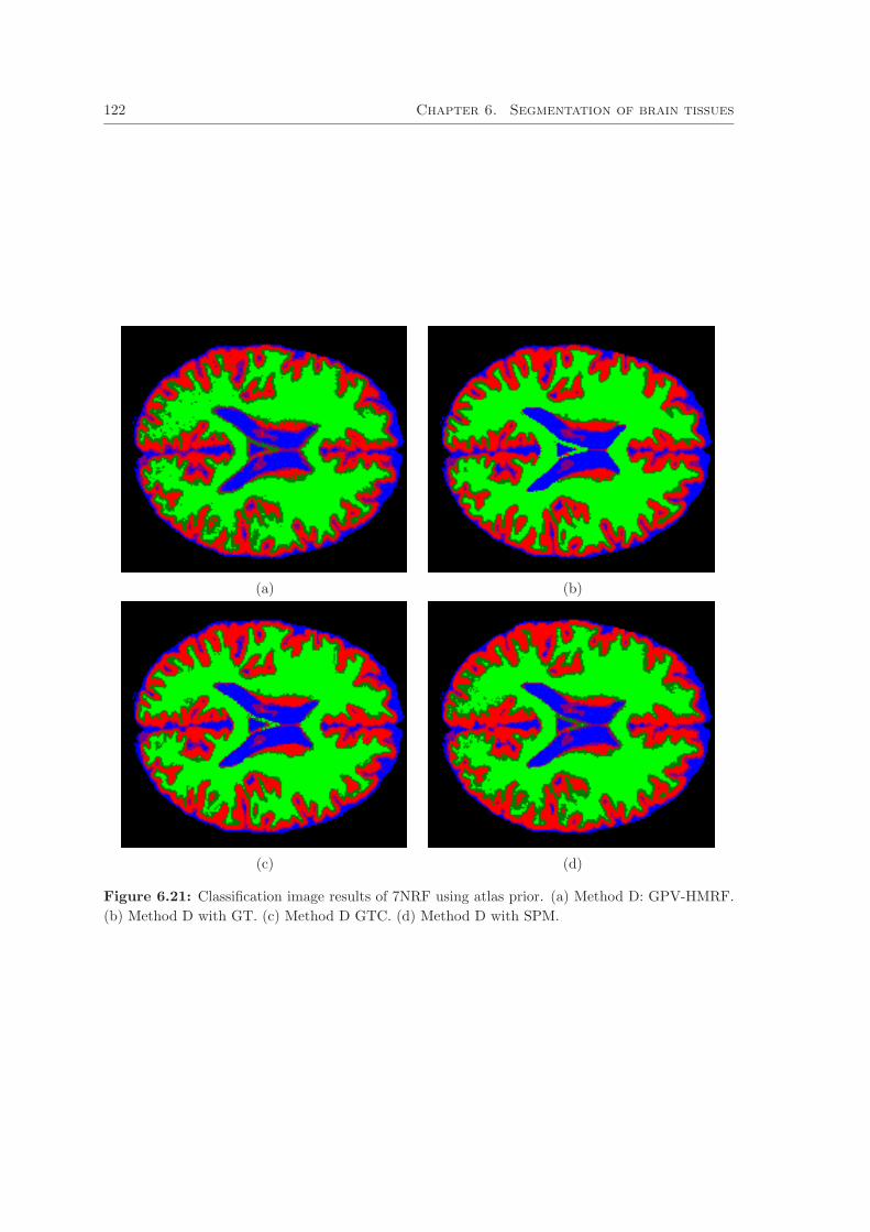
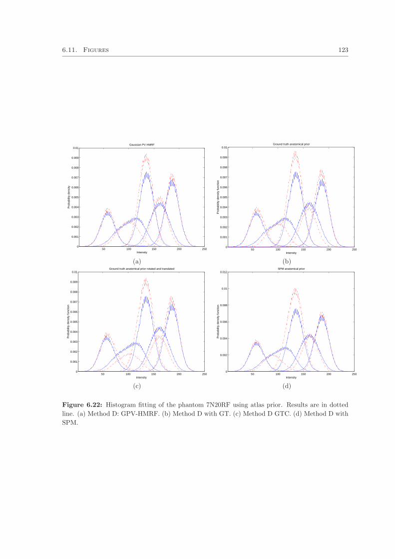
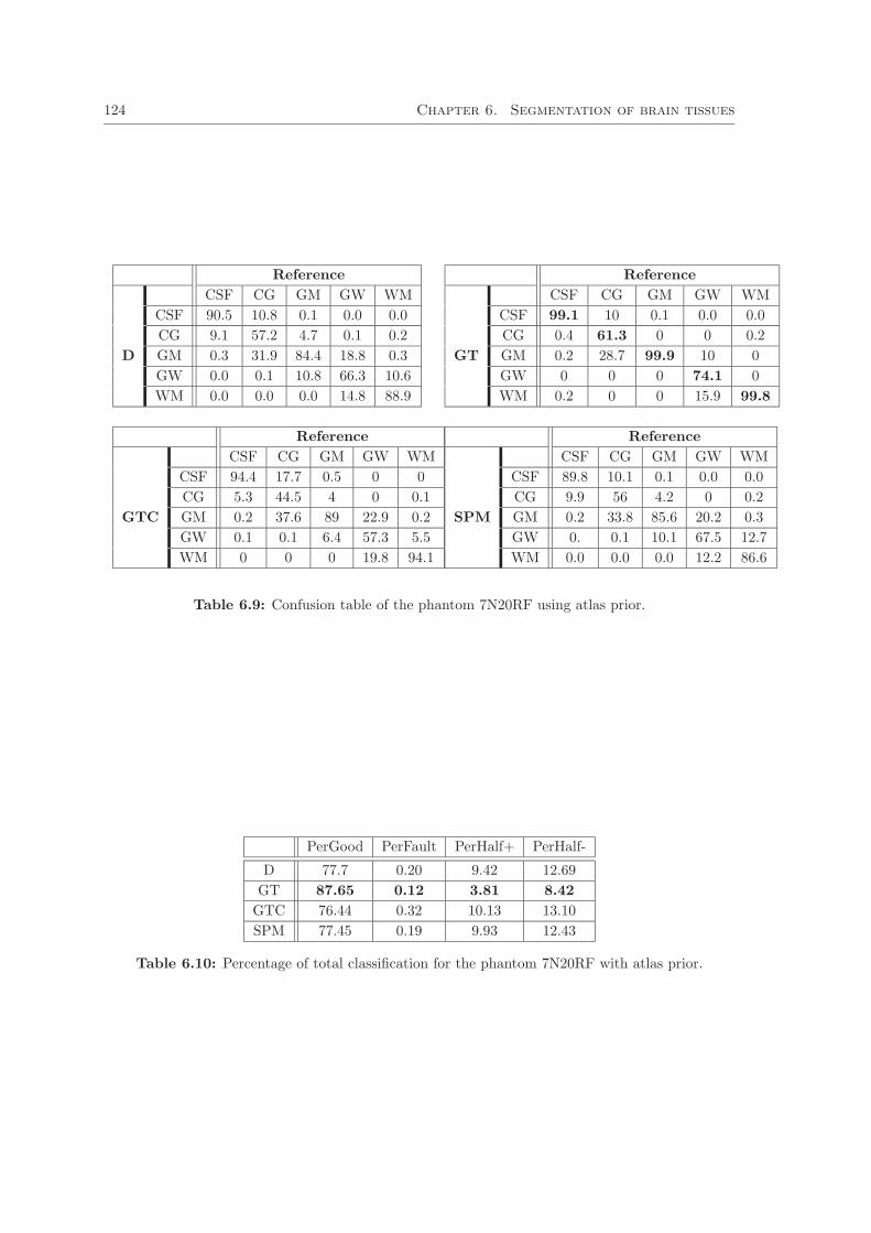
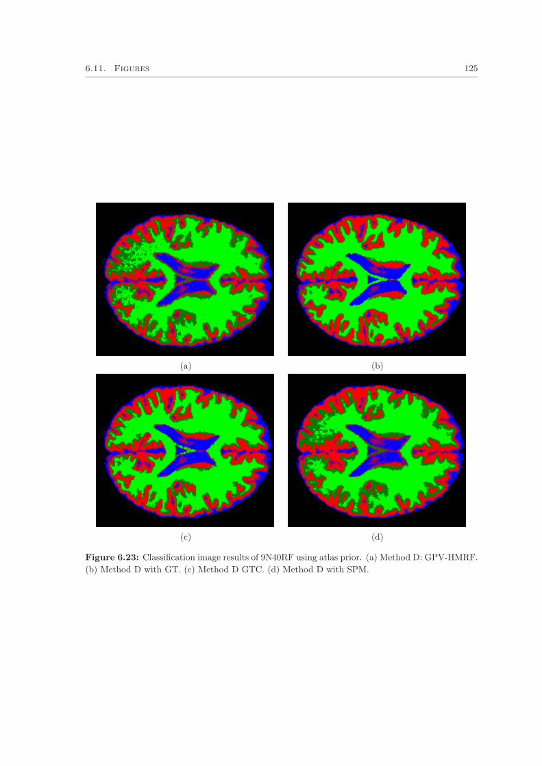
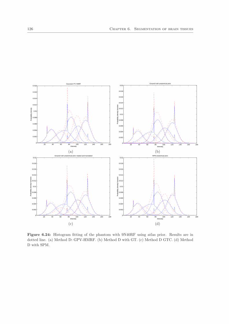
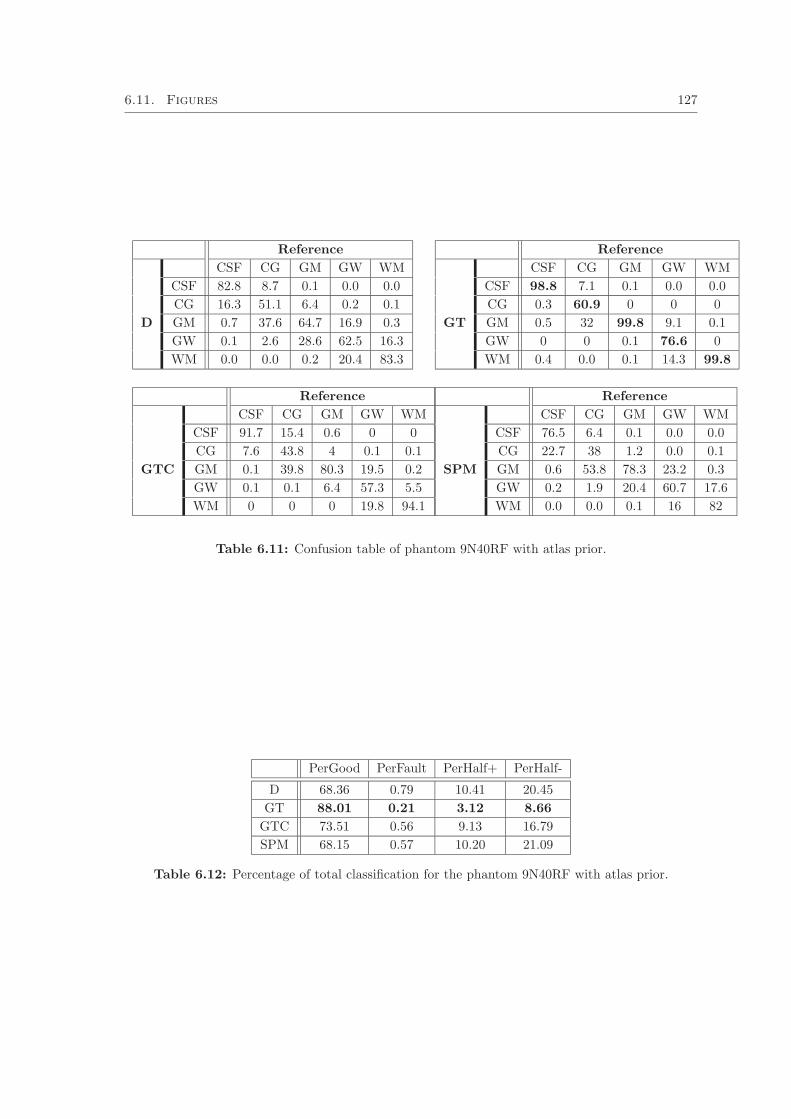
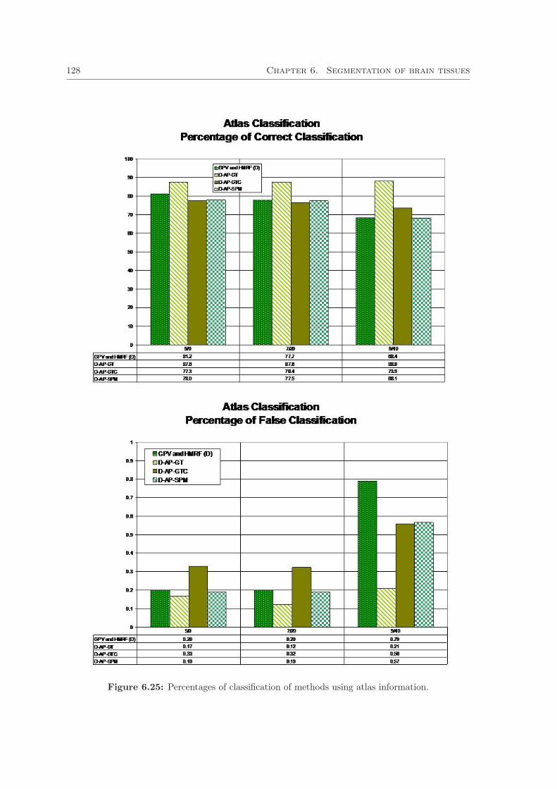


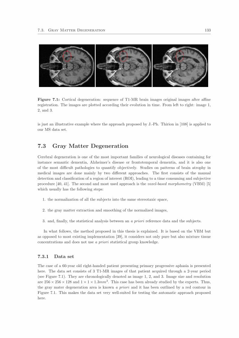
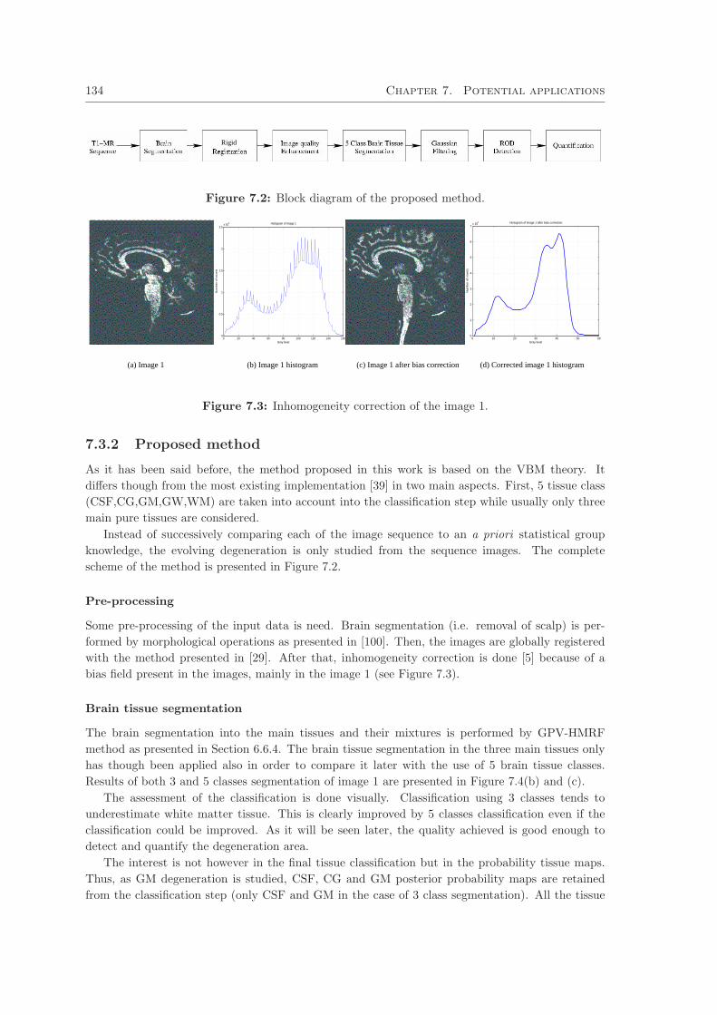
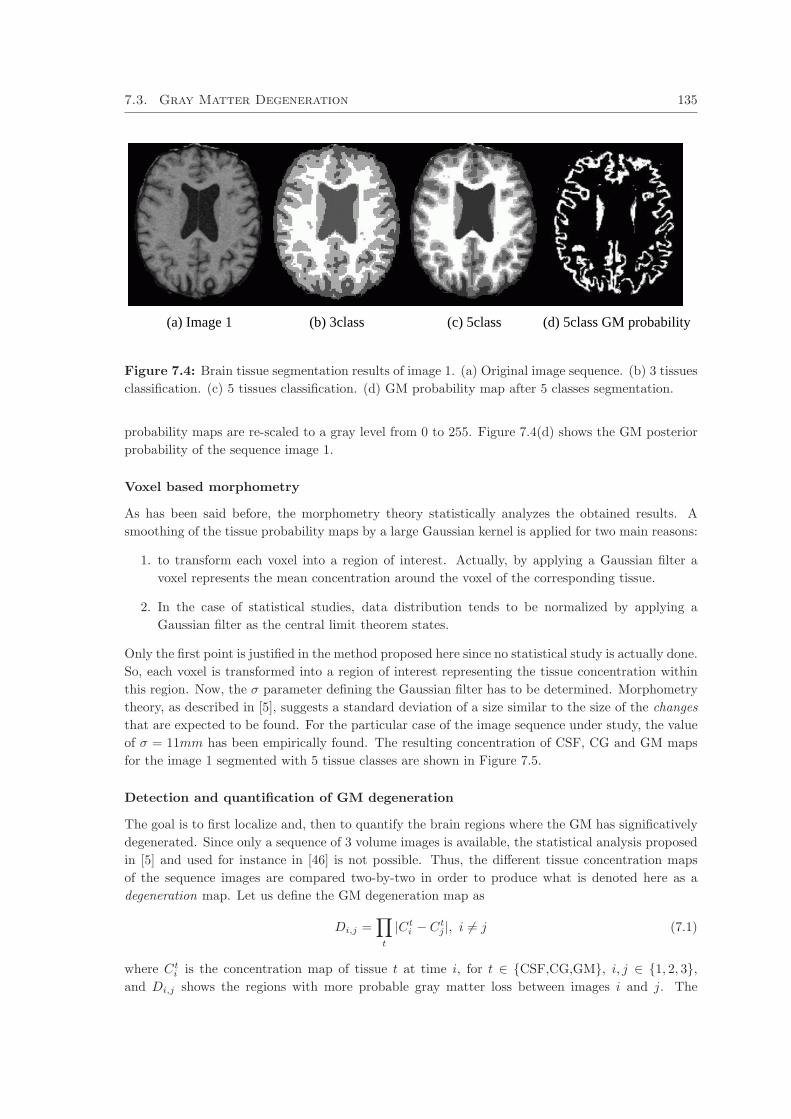
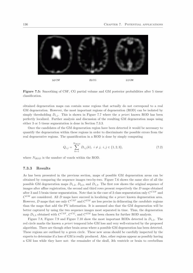
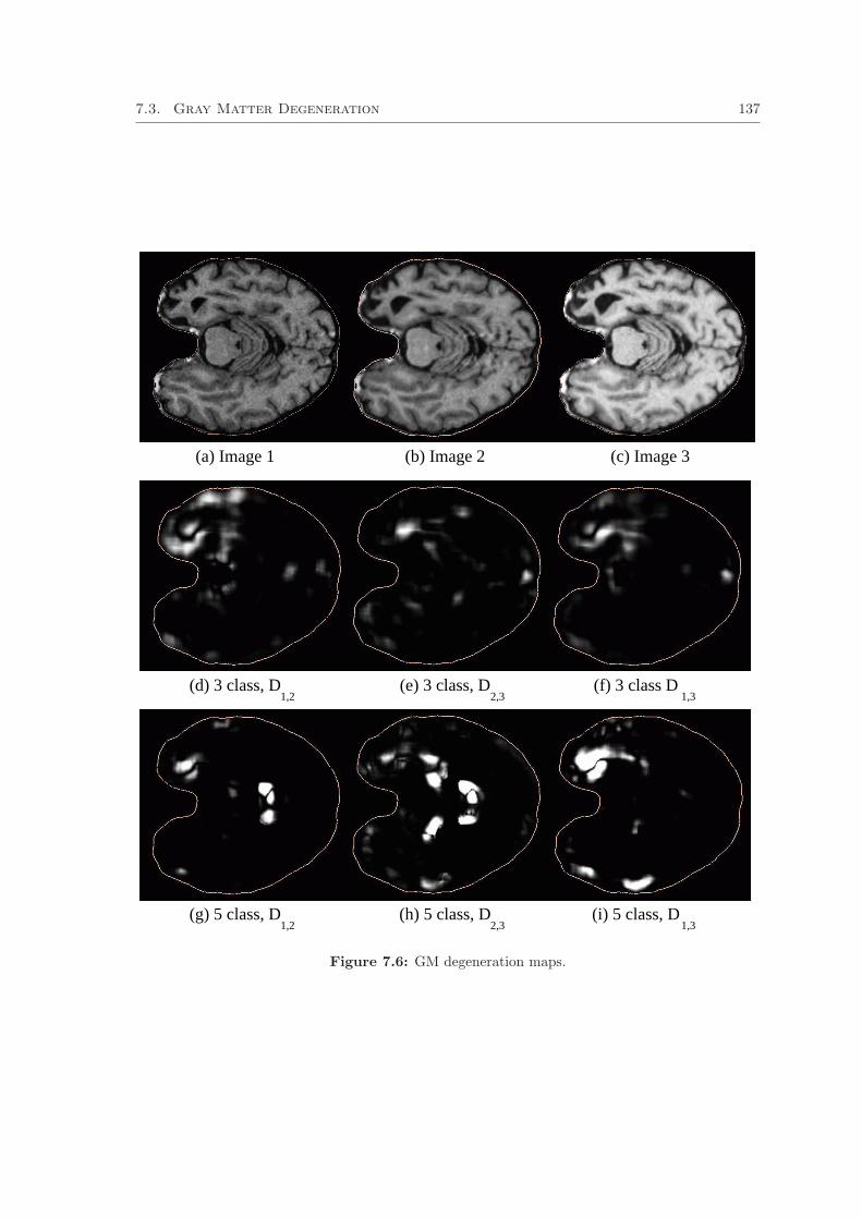
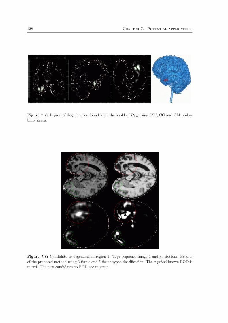
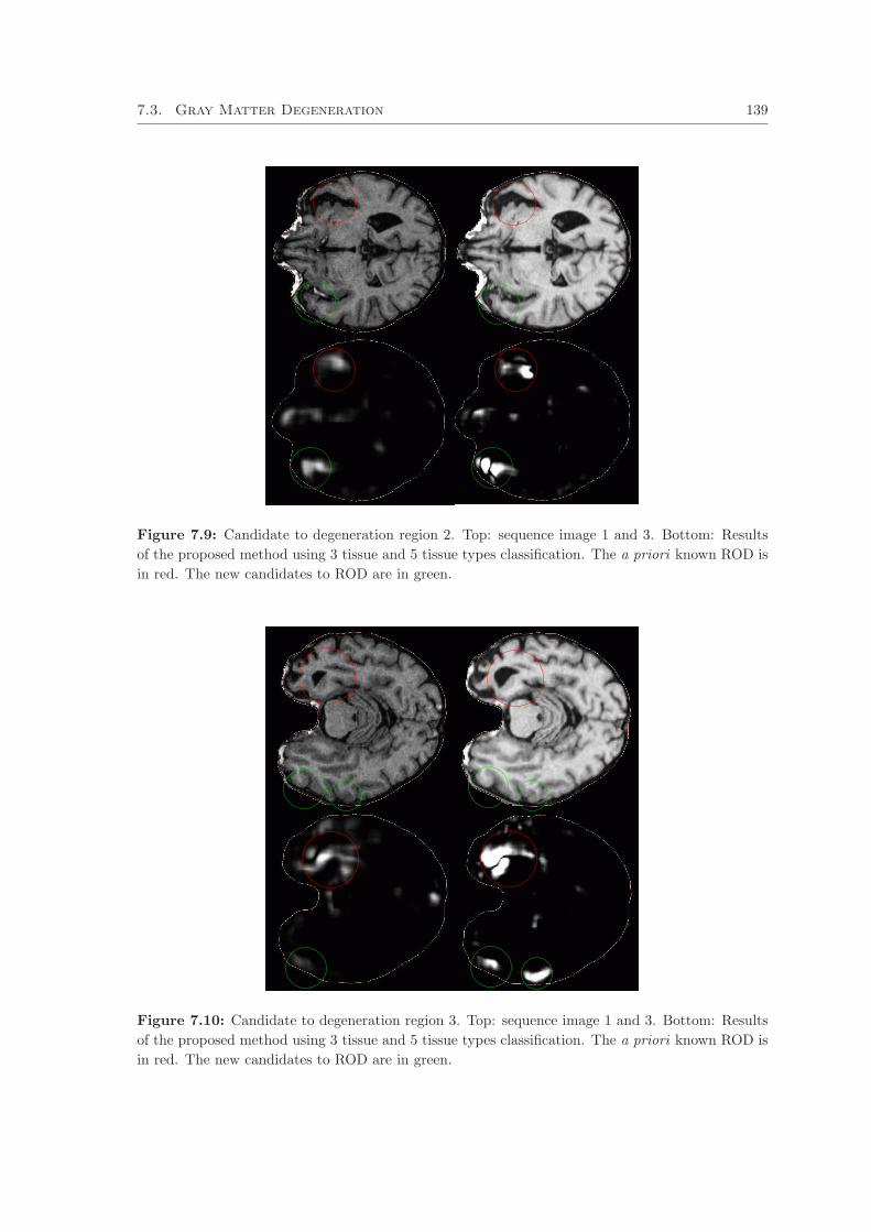
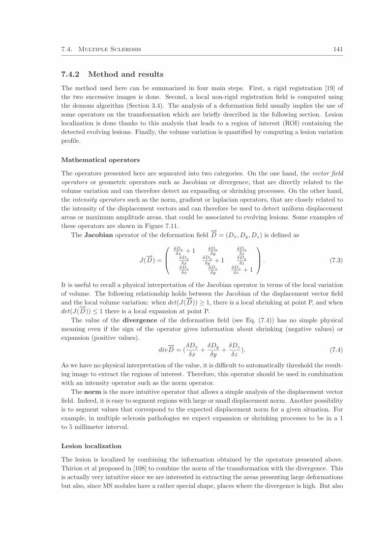
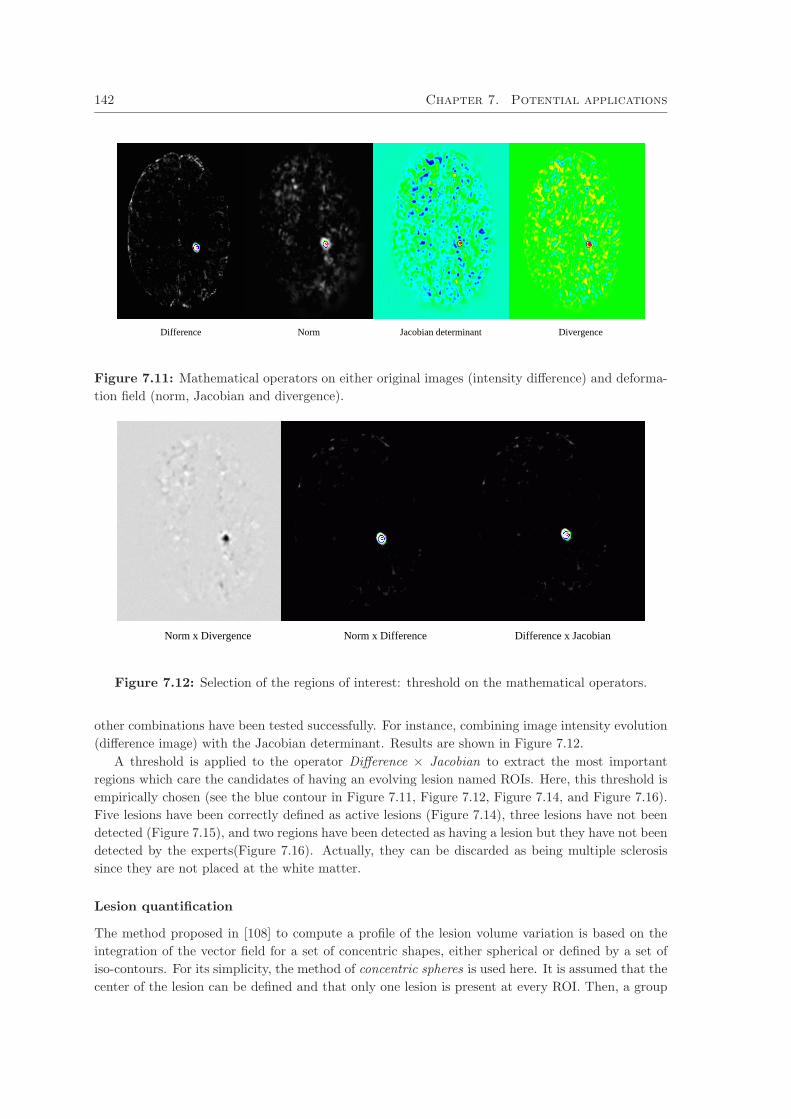
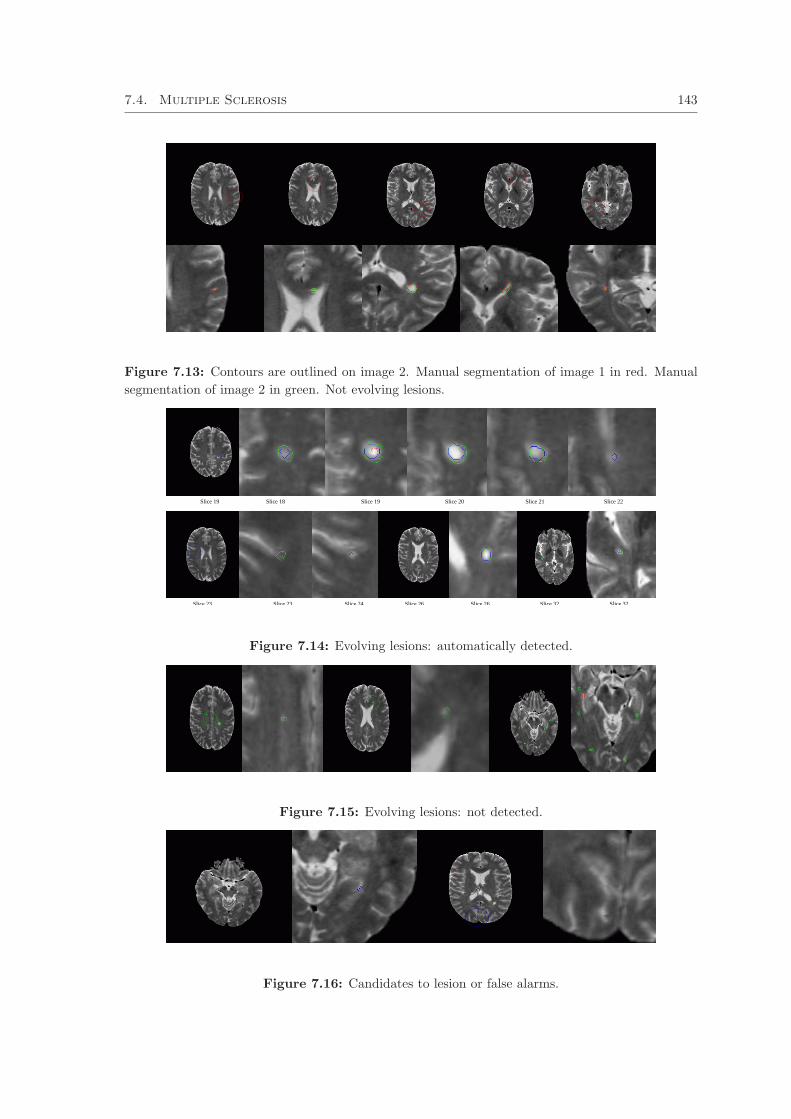
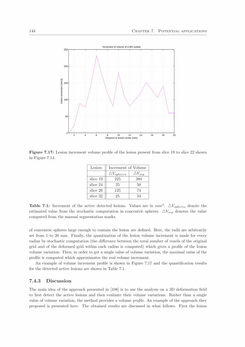


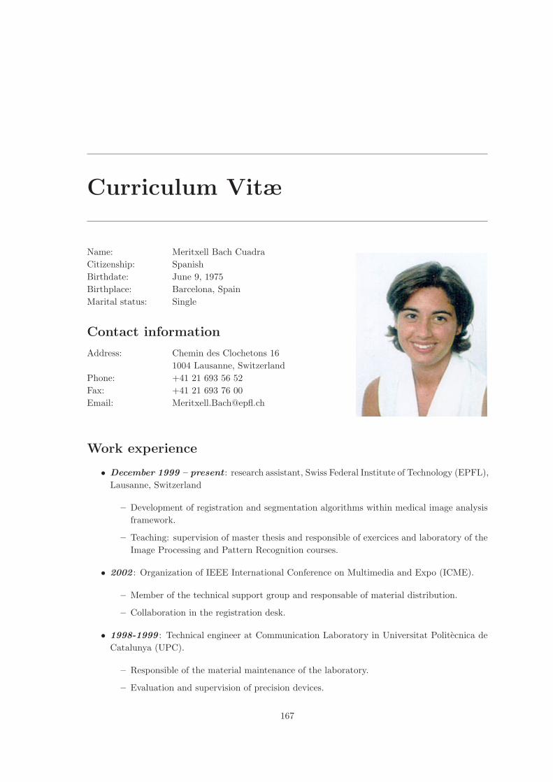


![" Atlas Renormalization for Improved Brain MR Image ... · Atlas Renormalization for Improved Brain MR Image Segmentation Across Scanner Platforms ... atlas registration [14]. ...](https://static.documents.pub/doc/80x56/5b64f1637f8b9af84b8ded07/-atlas-renormalization-for-improved-brain-mr-image-atlas-renormalization.jpg)


