146
FACHBEREICH MATHEMATIK UND NATURWISSENSCHAFTEN FACHGRUPPE P HYSIK B ERGISCHE UNIVERSITÄT WUPPERTAL November 2010 Prospects for t ¯ t resonance searches at ATLAS Tatjana Lenz
FACHBEREICH MATHEMATIK UND NATURWISSENSCHAFTENFACHGRUPPE PHYSIKBERGISCHE UNIVERSITÄT WUPPERTAL
November 2010
Prospects for tt resonancesearches at ATLAS
Tatjana Lenz

Diese Dissertation kann wie folgt zitiert werden: urn:nbn:de:hbz:468-20110414-094521-3 [http://nbn-resolving.de/urn/resolver.pl?urn=urn:nbn:de:hbz:468-20110414-094521-3]
Contents
1 Introduction 1
2 Theoretical Aspects of Top Quark Physics 32.1 Basic Concepts of the Standard Model . . . . . . . . . . . . . . . . . . . . . . . 32.2 Standard Model Top Quark Pair Production and Decay . . . . . . . . . . . . . 102.3 Top Quark Pair Production in the BSM Models . . . . . . . . . . . . . . . . . . 12
3 LHC and ATLAS Detector 193.1 The Large Hadron Collider . . . . . . . . . . . . . . . . . . . . . . . . . . . . . 193.2 The Atlas Detector . . . . . . . . . . . . . . . . . . . . . . . . . . . . . . . . . . 213.3 Forward Detectors . . . . . . . . . . . . . . . . . . . . . . . . . . . . . . . . . . 333.4 Data Acquisition System . . . . . . . . . . . . . . . . . . . . . . . . . . . . . . . 343.5 Performance of the LHC and the ATLAS Experiment . . . . . . . . . . . . . . 36
4 Event Simulation 394.1 Main Aspects of Monte Carlo Event Simulation . . . . . . . . . . . . . . . . . . 39
4.1.1 Parton Level Event Generators . . . . . . . . . . . . . . . . . . . . . . . 414.1.2 Multi-purpose Event Generators . . . . . . . . . . . . . . . . . . . . . . 42
4.2 Detector Simulation . . . . . . . . . . . . . . . . . . . . . . . . . . . . . . . . . . 434.2.1 Full Detector Simulation . . . . . . . . . . . . . . . . . . . . . . . . . . . 434.2.2 Fast Detector Simulation . . . . . . . . . . . . . . . . . . . . . . . . . . . 44
4.3 Signal and Background Event Modeling . . . . . . . . . . . . . . . . . . . . . . 454.3.1 Signal Event Simulation . . . . . . . . . . . . . . . . . . . . . . . . . . . 454.3.2 Background Event Simulation . . . . . . . . . . . . . . . . . . . . . . . 48
5 Event Reconstruction 535.1 Track Reconstruction in the Inner Detector . . . . . . . . . . . . . . . . . . . . 535.2 Primary Vertex Reconstruction . . . . . . . . . . . . . . . . . . . . . . . . . . . 555.3 Charged Lepton Identification . . . . . . . . . . . . . . . . . . . . . . . . . . . . 565.4 Jet Reconstruction . . . . . . . . . . . . . . . . . . . . . . . . . . . . . . . . . . . 595.5 Neutrino Reconstruction . . . . . . . . . . . . . . . . . . . . . . . . . . . . . . . 67
6 Topological Vertex Finder 716.1 Properties of b-Quark Jets . . . . . . . . . . . . . . . . . . . . . . . . . . . . . . 716.2 Association and Selection of Tracks and Jet Flavour Labelling . . . . . . . . . 746.3 b-Tagging Algorithms in ATLAS . . . . . . . . . . . . . . . . . . . . . . . . . . 776.4 Topological Vertex Finder . . . . . . . . . . . . . . . . . . . . . . . . . . . . . . 806.5 Secondary Vertex Reconstruction Performance . . . . . . . . . . . . . . . . . . 856.6 Application to b-Tagging . . . . . . . . . . . . . . . . . . . . . . . . . . . . . . . 88

4 Contents
6.7 Performance in Rejecting Light Quark Jets . . . . . . . . . . . . . . . . . . . . . 90
7 The tt Invariant Mass Distribution 937.1 Event Selection . . . . . . . . . . . . . . . . . . . . . . . . . . . . . . . . . . . . 937.2 Event Topology . . . . . . . . . . . . . . . . . . . . . . . . . . . . . . . . . . . . 997.3 Analysis Strategy . . . . . . . . . . . . . . . . . . . . . . . . . . . . . . . . . . . 1027.4 Selection Efficiency and Mass Resolution . . . . . . . . . . . . . . . . . . . . . 1057.5 Systematic Uncertainties . . . . . . . . . . . . . . . . . . . . . . . . . . . . . . . 1117.6 Resonance Width . . . . . . . . . . . . . . . . . . . . . . . . . . . . . . . . . . . 120
8 Heavy Resonance Searches at ATLAS 1238.1 Statistical Tools . . . . . . . . . . . . . . . . . . . . . . . . . . . . . . . . . . . . 1238.2 Sensitivity for Heavy Resonances . . . . . . . . . . . . . . . . . . . . . . . . . . 1258.3 Prospects for Heavy Resonance Searches . . . . . . . . . . . . . . . . . . . . . . 129
9 Summary and Conclusions 131

1 Introduction
What is the world made of? This is one of the fundamental questions scientists try to an-swer at the Large Hadron Collider (LHC) located at European Organization for NuclearResearch, near Geneva. The LHC is the world’s largest particle accelerator and collider. InDecember 2009 the LHC has started its operation and since then provides collisions for thefour main experiments. ATLAS is one of the general purpose experiments, it covers a broadrange of topics in high energy physics. This thesis has been performed within the ATLAScollaboration.
According to our current knowledge about the constituents of the matter, there are 12fundamental particles, 6 quarks and 6 leptons. While all ordinary matter is made of thelightest two quarks, the up and down quark, and the lightest charged lepton, the electron,the other particles can be produced in collisions of high-energy particles. The mass of par-ticles, although present in everyday’s life, is theoretically not fully understood. In the Stan-dard Model of high-energy particle physics the mass is generated through the mechanismof electroweak symmetry breaking induced by one Higgs field, producing one additionalparticle, the Higgs boson. Since no evidence for the Higgs boson has been found yet, al-ternative mechanisms of the mass generation are of interest. The top quark is the heaviestfundamental particle known so far and due to its large mass, it plays an important role inthese theories. Such models predict the existence of new heavy particles which couple totop quarks. This leads to an additional production mechanism of top quarks and should bevisible in the invariant mass distribution of the top quark pairs.
First searches for new heavy particles in top quark pairs events have been performedat the TEVATRON collider of the Fermi National Accelerator Laboratory. So far no evidencefor new particles was found. The higher centre-of-mass energy at the LHC allows to extendthese searches for the first time into the TeV-regime. In this thesis a method has been de-veloped, which is able to reconstruct top quarks in a broad range of transverse momenta,from top quarks at rest up to range of TeV. Based on the reconstructed invariant mass dis-tribution, a statistical analysis has been performed to estimate the sensitivity of the ATLASexperiment to detect new heavy particles in the early stage of the experiment.
Another aspect of this thesis is the implementation of a vertex reconstruction algorithmin the ATLAS software framework. Vertex reconstruction is an important tool in high en-ergy physics. It is essential for the identification of jets originating from bottom quarks, forlifetime measurements and flavour physics. Many interesting physics processes, for exam-ple top quark decays, contain bottom quarks in the final state, while background processescontain only up, down, strange or gluon jets. Thus, the identification of bottom jets canbe used to separate signal from the background. The relatively long lifetime of B hadrons(βγcτ = O(1) mm), produced during the hadronisation of bottom quarks, is unique andallows to distinguish bottom jets from other jets. In this thesis a sophisticated secondary

2 Chapter 1. Introduction
vertex reconstruction algorithm is presented, which exploits the structure of B hadron de-cays inside the jets. Its application to a bottom jet identification algorithm will be discussedand compared to the algorithms available in the ATLAS software.

2 Theoretical Aspects of Top QuarkPhysics
The Standard Model of elementary particle physics [1–10] provides a theoretical frameworkto describe the fundamental particles and their interactions. Since its formulation in the1960s and 1970s it has been tested by a large number of experiments up to energies ofO(100) GeV and so far no significant deviations from its predictions could be observed.Nevertheless the Standard Model is not a complete theory. It includes only the descriptionof three of the four fundamental forces in nature, the electromagnetism, the weak and thestrong force. The gravitation can not be explained within the framework of the StandardModel. Another open question is the origin of the particle masses. The so-called Higgsmechanism [11] provides the particle masses in the Standard Model, but it is not experi-mentally confirmed yet. There are several other theoretical models trying to answer thisquestion. One of the Standard Model particles, the top quark, often plays a special role insuch theories due to its high mass. They predict existence of new particles which couplepreferably to top quarks. To discover these particles is one of the exciting prospects at theLHC.
A brief phenomenological introduction into the basic concepts of the Standard Modelwill be given in the first section of this chapter followed by a detailed description of topquark pair production and decay mechanisms in the Standard Model. An overview of the-ories beyond the Standard Model (BSM) predicting resonant top quark pair production willbe given in the last section.
2.1 Basic Concepts of the Standard Model
All matter is build from quarks and leptons. The most well-known lepton is the electron.Quarks are constituents of protons and neutrons. Quarks and leptons are spin- 1
2 particles,so-called fermions, and obey Fermi-Dirac statistics as well as the Pauli exclusion principle.For each kind of particle there exists a corresponding antiparticle with identical proper-ties except for the reversal of their quantum numbers, which describes values of conservedquantities. Fermions are subdivided into three generations. Each generation is identical intheir attributes except their masses. The first generation of quarks and leptons: up (u) anddown (d) quarks, electron (e) and electron-neutrino (νe) build all known matter. The secondand third generations: charm (c) and strange (s) quarks, muon (µ) and muon-neutrino (νµ),top (t) and bottom (b) quarks, tau (τ) and tau-neutrino (ντ) can only be observed in high-energy interactions since they subsequently decay into first generation particles. Chargedleptons (e, µ, τ) carry one elementary charge, while the corresponding neutrinos are neu-tral. The quarks carry fractional electric charges, the up-type (u, c, t) quarks +2/3 and the

4 Chapter 2. Theoretical Aspects of Top Quark Physics
down-type (d, s, b) quarks -1/3 of the elementary charge. All but top quarks are bound incombinations of quarks and antiquarks, so-called hadrons, with integer charge. Hadronsbuild of three quarks are baryons, the quark-antiquark states are mesons. Without an addi-tional quantum number the Pauli principle would be violated for qqq-states. Thus, quarkscarry colour charge denoted as red, green and blue.
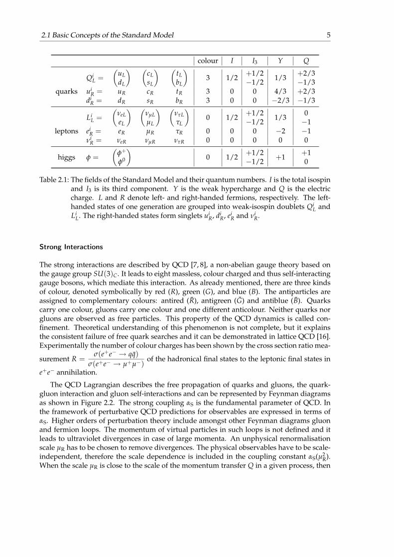
Fermions interact by four fundamental interactions: the electromagnetic force, the weakand the strong force and the gravitation. The gravitation can be neglected in high-energyphysics, because its strength is about 43 orders of magnitude weaker than the strong inter-action. The mediators of the interactions between fermions are gauge bosons. The gaugebosons have integer spin and obey Bose-Einstein statistics. Eight gauge bosons, so-calledgluons, belong to quantum chromodynamics (QCD) that describes strong interactions. Thequantum number of QCD is the already introduced colour charge. The mediators of theelectromagnetic and weak interactions are photons (γ) and Z- and W±-bosons. From a his-torical point of view, quantum electrodynamics (QED) was the first formulated gauge theoryto describe electromagnetic interactions mediated by photons. Later Glashow, Weinberg andSalam [1, 4–6, 12] have succeeded to combine the description of weak and electromagneticinteractions in one gauge theory and herewith to allow a proper description of the weak in-teraction. The electro-weak quantum numbers are weak isospin ~T and hypercharge Y. Theleft-handed fermions have the total weak-isospin T = 1/2 and form weak-isospin doublets.The right-handed fermions have T = 0 and form singlets. The electric charge is related to thethird component of the weak-isospin T3 and the weak hypercharge by Q = T3 + Y/2. Thecharged leptons interact electromagnetically and weakly, the neutral leptons interact onlyweakly. By contrast, the quarks interact via all three interactions: electromagnetic, weakand strong. All fundamental particles and some of their properties are shown in Figure 2.1.
QCD and the electro-weak theory are relativistic quantum field gauge theories, whichare combined into the Standard Model. The Standard Model is a gauge theory based on theset of fields, namely three generations of fermions, one Higgs field and the gauge fields ofSU(3)C × SU(2)L ×U(1)Y symmetry group as listed in Table 2.1. SU(3)C is the symmetrygroup of the strong interaction, SU(2)L of the weak interaction and U(1)Y of the electromag-netic interaction. The symmetry transformations can be performed both locally and glob-ally. Each gauge symmetry is connected to the conservation of a corresponding quantumnumber, as stated by the Noether theorem [13]. In a gauge theory, the Lagrangian, whichdescribes the dynamics of a physical system, is invariant under local gauge transforma-tions. Gauge fields guarantee this invariance and the excitatitions of these fields representthe particles transmitting the forces, the gauge bosons. To obtain massive gauge bosons,the introduction of a mass term into the Lagrangian is necessary. Such a term is not gaugeinvariant under local gauge transformations. A solution has been provided by Higgs [11],who introduced a new scalar field, named then Higgs field. The non-zero vacuum expecta-tion value of the Higgs field breaks spontaneously the electro-weak symmetry. This leads tothe emergence of the massive vector bosons, the W and Z bosons, and a massless photon.In the following, all three interactions as well as the Higgs mechanisms will be explained inmore details.
2.1 Basic Concepts of the Standard Model 5
colour I I3 Y Q
QiL =
(uLdL
) (cLsL
) (tLbL
)3 1/2
+1/2−1/2
1/3+2/3−1/3
quarks uiR = uR cR tR 3 0 0 4/3 +2/3
diR = dR sR bR 3 0 0 −2/3 −1/3
LiL =
(νeLeL
) (νµLµL
) (ντLτL
)0 1/2
+1/2−1/2
1/30−1
leptons eiR = eR µR τR 0 0 0 −2 −1
νiR = νeR νµR ντR 0 0 0 0 0
higgs φ =(
φ+
φ0
)0 1/2
+1/2−1/2
+1+10
Table 2.1: The fields of the Standard Model and their quantum numbers. I is the total isospinand I3 is its third component. Y is the weak hypercharge and Q is the electriccharge. L and R denote left- and right-handed fermions, respectively. The left-handed states of one generation are grouped into weak-isospin doublets Qi
L andLi
L. The right-handed states form singlets uiR, di
R, eiR and νi
R.
Strong Interactions
The strong interactions are described by QCD [7, 8], a non-abelian gauge theory based onthe gauge group SU(3)C. It leads to eight massless, colour charged and thus self-interactinggauge bosons, which mediate this interaction. As already mentioned, there are three kindsof colour, denoted symbolically by red (R), green (G), and blue (B). The antiparticles areassigned to complementary colours: antired (R), antigreen (G) and antiblue (B). Quarkscarry one colour, gluons carry one colour and one different anticolour. Neither quarks norgluons are observed as free particles. This property of the QCD dynamics is called con-finement. Theoretical understanding of this phenomenon is not complete, but it explainsthe consistent failure of free quark searches and it can be demonstrated in lattice QCD [16].Experimentally the number of colour charges has been shown by the cross section ratio mea-
surement R =σ(e+e− → qq)
σ(e+e− → µ+µ−)of the hadronical final states to the leptonic final states in
e+e− annihilation.
The QCD Lagrangian describes the free propagation of quarks and gluons, the quark-gluon interaction and gluon self-interactions and can be represented by Feynman diagramsas shown in Figure 2.2. The strong coupling αS is the fundamental parameter of QCD. Inthe framework of perturbative QCD predictions for observables are expressed in terms ofαS. Higher orders of perturbation theory include amongst other Feynman diagrams gluonand fermion loops. The momentum of virtual particles in such loops is not defined and itleads to ultraviolet divergences in case of large momenta. An unphysical renormalisationscale µR has to be chosen to remove divergences. The physical observables have to be scale-independent, therefore the scale dependence is included in the coupling constant αS(µ2
R).When the scale µR is close to the scale of the momentum transfer Q in a given process, then

6 Chapter 2. Theoretical Aspects of Top Quark Physics
GAUGE BOSONS
LEPTONSQUARKS
in the units
+2/3
in MeV
0 0 0 0
−1
−1
0
FERMIONS
−1/3
−1/3
−1/3
+2/3
+2/3
of the fundamentalelectric charge
0Charge Mass
105.7
1776.8
Symbol
Name
< 0.002
< 0.002
91187.6
Spin
+_ 1
1111
1/2
1/2
1/2
1/2
1/2
1/2
1/2 1/2
1/2 1/2
1/2 1/2
intrinsic angularmomentum
Colour
colourcharge
µmuon
νµ
τtau
up
du
c scharm strange
down
t btop bottom
ggluon
0
photon
γ W Z000
80398
0
3 3
3 3
33
0 0
0
0
0
0
neutrinomuon−
tau−neutrino
ντ
weak bosons
−1 0.511 0 < 0.002
e νeelectron−
neutrinoelecton
8 0
hhiggs
0 ?
101
4190
4.1−5.81.7−3.3
1270
173300
Figure 2.1: Fundamental particles of the Standard Model [14]. Top quark mass is taken fromReference [15].
q g
gq
q
g
g
g
g g
g g
Figure 2.2: Elements of Feynman diagrams in QCD: propagators for quarks and gluons,quark-gluon vertex, three and four gluon vertex.
αS(µ2R ≈ Q2) is indicative of the effective strength of the interaction in that process. The
scale dependence of the renormalised coupling constant is controlled by the renormalisa-tion group equations. In first order perturbation theory αS(Q2) has the form (corresponding
2.1 Basic Concepts of the Standard Model 7
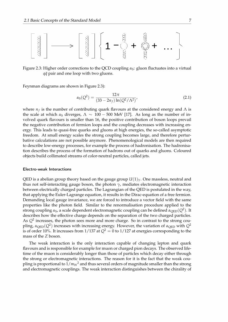
1 − ...+ +
Figure 2.3: Higher order corrections to the QCD coupling αS: gluon fluctuates into a virtualqq pair and one loop with two gluons.
Feynman diagrams are shown in Figure 2.3):
αS(Q2) =12π
(33− 2n f ) ln(Q2/Λ2), (2.1)
where n f is the number of contributing quark flavours at the considered energy and Λ isthe scale at which αS diverges, Λ ∼ 100 − 500 MeV [17]. As long as the number of in-volved quark flavours is smaller than 16, the positive contribution of boson loops prevailthe negative contribution of fermion loops and the coupling decreases with increasing en-ergy. This leads to quasi-free quarks and gluons at high energies, the so-called asymptoticfreedom. At small energy scales the strong coupling becomes large, and therefore pertur-bative calculations are not possible anymore. Phenomenological models are then requiredto describe low-energy processes, for example the process of hadronisation. The hadronisa-tion describes the process of the formation of hadrons out of quarks and gluons. Colouredobjects build collimated streams of color-neutral particles, called jets.
Electro-weak Interactions
QED is a abelian group theory based on the gauge group U(1)Y. One massless, neutral andthus not self-interacting gauge boson, the photon γ, mediates electromagnetic interactionbetween electrically charged particles. The Lagrangian of the QED is postulated in the way,that applying the Euler-Lagrange equation, it results in the Dirac-equation of a free fermion.Demanding local gauge invariance, we are forced to introduce a vector field with the sameproperties like the photon field. Similar to the renormalisation procedure applied to thestrong coupling αS, a scale dependent electromagnetic coupling can be defined αQED(Q2). Itdescribes how the effective charge depends on the separation of the two charged particles.As Q2 increases, the photon sees more and more charge. So in contrast to the strong cou-pling, αQED(Q2) increases with increasing energy. However, the variation of αQED with Q2
is of order 10%. It increases from 1/137 at Q2 = 0 to 1/127 at energies corresponding to themass of the Z boson.
The weak interaction is the only interaction capable of changing lepton and quarkflavours and is responsible for example for muon or charged pion decays. The observed life-time of the muon is considerably longer than those of particles which decay either throughthe strong or electromagnetic interactions. The reason for it is the fact that the weak cou-pling is proportional to 1/mW
2 and thus several orders of magnitude smaller than the strongand electromagnetic couplings. The weak interaction distinguishes between the chirality of
8 Chapter 2. Theoretical Aspects of Top Quark Physics
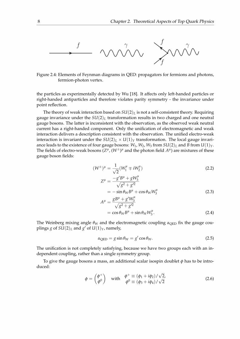
γ γff
f
Figure 2.4: Elements of Feynman diagrams in QED: propagators for fermions and photons,fermion-photon vertex.
the particles as experimentally detected by Wu [18]. It affects only left-handed particles orright-handed antiparticles and therefore violates parity symmetry - the invariance underpoint reflection.
The theory of weak interaction based on SU(2)L is not a self-consistent theory. Requiringgauge invariance under the SU(2)L transformation results in two charged and one neutralgauge bosons. The latter is inconsistent with the observation, as the observed weak neutralcurrent has a right-handed component. Only the unification of electromagnetic and weakinteraction delivers a description consistent with the observation. The unified electro-weakinteraction is invariant under the SU(2)L ×U(1)Y transformation. The local gauge invari-ance leads to the existence of four gauge bosons: W1, W2, W3 from SU(2)L and B from U(1)Y.The fields of electro-weak bosons (Zµ, (W±)µ and the photon field Aµ) are mixtures of thesegauge boson fields:
(W±)µ =1√2(Wµ
1 ∓ iWµ2 ) (2.2)
Zµ =−g′Bµ + gWµ
3√g2 + g′2
= − sin θW Bµ + cos θWWµ3 (2.3)
Aµ =gBµ + g′Wµ
3√g2 + g′2
= cos θW Bµ + sin θWWµ3 . (2.4)
The Weinberg mixing angle θW and the electromagnetic coupling αQED fix the gauge cou-plings g of SU(2)L and g′ of U(1)Y, namely,
αQED = g sin θW = g′ cos θW . (2.5)
The unification is not completely satisfying, because we have two groups each with an in-dependent coupling, rather than a single symmetry group.
To give the gauge bosons a mass, an additional scalar isospin doublet φ has to be intro-duced:
φ =(
φ+
φ0
)with
φ+ ≡ (φ1 + iφ2)/√
2,φ0 ≡ (φ3 + iφ4)/
√2
(2.6)
2.1 Basic Concepts of the Standard Model 9
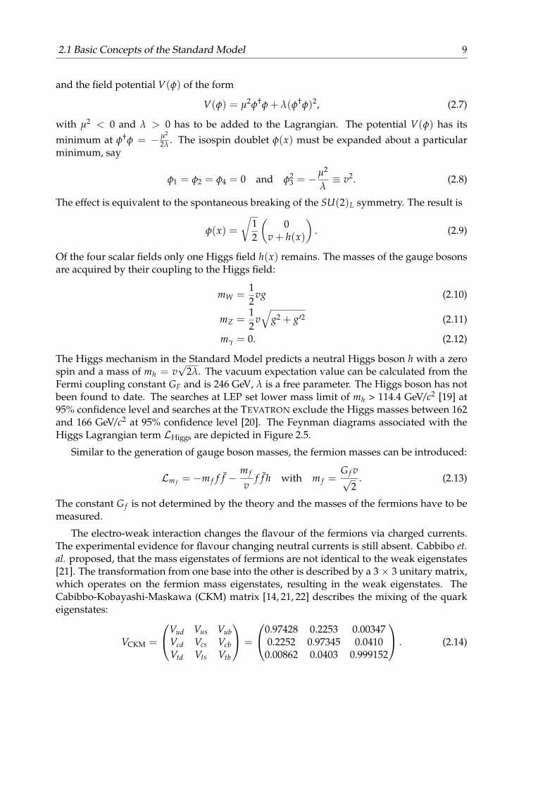
and the field potential V(φ) of the form
V(φ) = µ2φ†φ + λ(φ†φ)2, (2.7)
with µ2 < 0 and λ > 0 has to be added to the Lagrangian. The potential V(φ) has itsminimum at φ†φ = − µ2
2λ . The isospin doublet φ(x) must be expanded about a particularminimum, say
φ1 = φ2 = φ4 = 0 and φ23 = −µ2
λ≡ v2. (2.8)
The effect is equivalent to the spontaneous breaking of the SU(2)L symmetry. The result is
φ(x) =
√12
(0
v + h(x)
). (2.9)
Of the four scalar fields only one Higgs field h(x) remains. The masses of the gauge bosonsare acquired by their coupling to the Higgs field:
mW =12
vg (2.10)
mZ =12
v√
g2 + g′2 (2.11)
mγ = 0. (2.12)
The Higgs mechanism in the Standard Model predicts a neutral Higgs boson h with a zerospin and a mass of mh = v
√2λ. The vacuum expectation value can be calculated from the
Fermi coupling constant GF and is 246 GeV, λ is a free parameter. The Higgs boson has notbeen found to date. The searches at LEP set lower mass limit of mh > 114.4 GeV/c2 [19] at95% confidence level and searches at the TEVATRON exclude the Higgs masses between 162and 166 GeV/c2 at 95% confidence level [20]. The Feynman diagrams associated with theHiggs Lagrangian term LHiggs are depicted in Figure 2.5.
Similar to the generation of gauge boson masses, the fermion masses can be introduced:
Lm f = −m f f f −m f
vf f h with m f =
G f v√
2. (2.13)
The constant G f is not determined by the theory and the masses of the fermions have to bemeasured.
The electro-weak interaction changes the flavour of the fermions via charged currents.The experimental evidence for flavour changing neutral currents is still absent. Cabbibo et.al. proposed, that the mass eigenstates of fermions are not identical to the weak eigenstates[21]. The transformation from one base into the other is described by a 3 × 3 unitary matrix,which operates on the fermion mass eigenstates, resulting in the weak eigenstates. TheCabibbo-Kobayashi-Maskawa (CKM) matrix [14, 21, 22] describes the mixing of the quarkeigenstates:
VCKM =
Vud Vus VubVcd Vcs VcbVtd Vts Vtb
=
0.97428 0.2253 0.003470.2252 0.97345 0.04100.00862 0.0403 0.999152
. (2.14)
10 Chapter 2. Theoretical Aspects of Top Quark Physics
h hh
h
h
h
h
h
W,Z W,Zh
W,Z
h h
W,Z W,Z
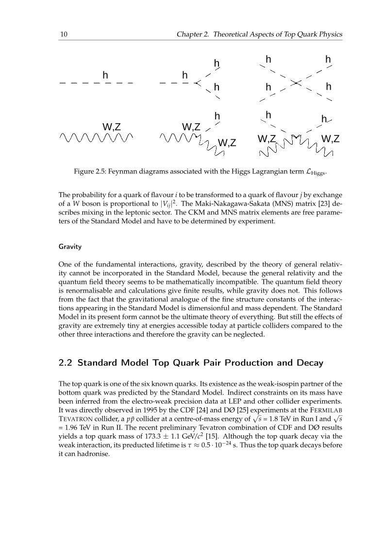
Figure 2.5: Feynman diagrams associated with the Higgs Lagrangian term LHiggs.
The probability for a quark of flavour i to be transformed to a quark of flavour j by exchangeof a W boson is proportional to |Vij|2. The Maki-Nakagawa-Sakata (MNS) matrix [23] de-scribes mixing in the leptonic sector. The CKM and MNS matrix elements are free parame-ters of the Standard Model and have to be determined by experiment.
Gravity
One of the fundamental interactions, gravity, described by the theory of general relativ-ity cannot be incorporated in the Standard Model, because the general relativity and thequantum field theory seems to be mathematically incompatible. The quantum field theoryis renormalisable and calculations give finite results, while gravity does not. This followsfrom the fact that the gravitational analogue of the fine structure constants of the interac-tions appearing in the Standard Model is dimensionful and mass dependent. The StandardModel in its present form cannot be the ultimate theory of everything. But still the effects ofgravity are extremely tiny at energies accessible today at particle colliders compared to theother three interactions and therefore the gravity can be neglected.
2.2 Standard Model Top Quark Pair Production and Decay
The top quark is one of the six known quarks. Its existence as the weak-isospin partner of thebottom quark was predicted by the Standard Model. Indirect constraints on its mass havebeen inferred from the electro-weak precision data at LEP and other collider experiments.It was directly observed in 1995 by the CDF [24] and DØ [25] experiments at the FERMILAB
TEVATRON collider, a pp collider at a centre-of-mass energy of√
s = 1.8 TeV in Run I and√
s= 1.96 TeV in Run II. The recent preliminary Tevatron combination of CDF and DØ resultsyields a top quark mass of 173.3 ± 1.1 GeV/c2 [15]. Although the top quark decay via theweak interaction, its preducted lifetime is τ ≈ 0.5 · 10−24 s. Thus the top quark decays beforeit can hadronise.

2.2 Standard Model Top Quark Pair Production and Decay 11
Top Quark Production
The dominating production mechanism for top quarks at hadron colliders is via the stronginteraction in pairs [26], while the single top quark production mediated by the electro-weak interaction has subleading character [27]. The underlying theoretical framework forthe calculation of the production cross sections at hadron colliders is the QCD-improvedparton model [28]. The colliding high-energy hadrons are considered as a composition ofthe quasi-free quarks and gluons, so-called partons. Each parton i carries a fraction xi ofthe hadron momentum pA. The parton distribution functions (PDFs) fi/A(xi, µ2) describesthe probability density to find a parton of a flavour i inside the hadron A carrying the mo-mentum fraction xi. The production cross section is calculated as a convolution of the PDFsfi/A(xi, µ2) and f j/B(xj, µ2) for the hadrons A and B and the parton-parton cross sectionσij(ij→ tt):
σ(AB→ tt) = ∑i,j=q,q,g
∫dxidxj fi/A(xi, µ2) f j/B(xj, µ2)σij(ij→ tt; s, µ2), (2.15)
where s is the square root of the centre-of-mass energy of colliding partons and µ denotesthe typical energy scale of the considered interaction. The partonic tt production cross sec-tion can be calculated in perturbative QCD. The Feynman diagrams of the leading ordersubprocesses are depicted in Figure 2.7, contributing in α2
S to the perturbation series. Figure2.6 shows exemplary the parton distribution functions for u, u, d, d, s quarks and gluonsinside the proton in the CTEQ6.6M [29] parametrisation evaluated at µ = 175 GeV. The en-ergy of partons has to be at least large enough to produce top quark pairs at rest s & 4m2
t .Together with the approximation xi ≈ xj, this leads to a typical parton momentum value xfor the tt production at the kinematic threshold x ≈ 2mt/
√s, where s is the centre-of-mass
energy of colliding protons. The typical value at the LHC with a centre-of-mass energy of10 TeV is x ≈ 0.03 and thus the dominant production mechanism at the LHC is gluon-gluonfusion with about 90% contribution. The tt production cross section at LHC is predictedto be 402+19
−26 pb at 10 TeV for mt = 172.5 GeV/c2 and CTEQ6.6 PDF parametrisation [26].The quoted uncertainties include the uncertainty due to the choice of the scale µ and theuncertainty associated with the PDF parametrisation.
Top Quark Decay
The top quark decays via the weak interaction in a W boson and a down-type quark. Thedecay rates are proportional to the CKM matrix elements |Vtq|2 with q = d, s, b quarks.Under assumption of the unitarity of the three generation CKM matrix, the matrix element|Vtb| is nearly 1, and thus the decay rate t→W+ b is nearly 100%. The mass of the top quarkis high enough to produce real W bosons and the decay width of the top quarks is extremelylarge [30]:
Γ(t→Wb) ≈ 1.42 GeV for mt = 175 GeV/c2, (2.16)
that implies a very short lifetime of ∼ 0.5 · 10−24 s. The characteristic formation time ofhadrons is τform ≈ 3 · 10−24 s. Therefore the top quark decays prior to hadronisation.
12 Chapter 2. Theoretical Aspects of Top Quark Physics
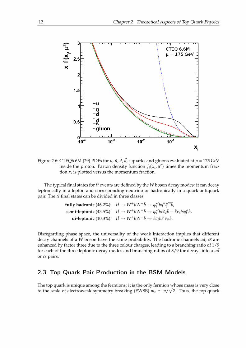
Figure 2.6: CTEQ6.6M [29] PDFs for u, u, d, d, s quarks and gluons evaluated at µ = 175 GeVinside the proton. Parton density function fi(xi, µ2) times the momentum frac-tion xi is plotted versus the momentum fraction.
The typical final states for tt events are defined by the W boson decay modes: it can decayleptonically in a lepton and corresponding neutrino or hadronically in a quark-antiquarkpair. The tt final states can be divided in three classes:
fully hadronic (46.2%): tt→W+bW−b→ qq′bq′′q′′′b,semi-leptonic (43.5%): tt→W+bW−b→ qq′b`ν`b + ¯ν`bqq′b,
di-leptonic (10.3%): tt→W+bW−b→ `ν`b`′ν`′ b.
Disregarding phase space, the universality of the weak interaction implies that differentdecay channels of a W boson have the same probability. The hadronic channels ud, cs areenhanced by factor three due to the three colour charges, leading to a branching ratio of 1/9for each of the three leptonic decay modes and branching ratios of 3/9 for decays into a udor cs pairs.
2.3 Top Quark Pair Production in the BSM Models
The top quark is unique among the fermions: it is the only fermion whose mass is very closeto the scale of electroweak symmetry breaking (EWSB) mt ' v/
√2. Thus, the top quark

2.3 Top Quark Pair Production in the BSM Models 13
q
q
g
t
t
g
g
g
t
t
g
g
g
g
t
t
t
t
t
t
Figure 2.7: tt production channels at leading order perturbation theory.
has been exploited in many scenarios of the fermion and boson mass generation beyond theStandard Model. For example it triggers the mechanism of EWSB in the supersymmetricmodels (SUSY) or it plays an important role in many alternative mechanisms of the massgeneration. These models predict the existence of new heavy particles, which couple to thetop quarks. This leads to an additional non-QCD production mechanism for the top quarkpairs. In the following, an overview of the models predicting neutral s-channel resonanceswill be given as well as experimental constraints on these models. The list of the modelsis not complete and exemplifies only possible theories. A generic neutral colour singletresonance will be discussed in more details.
In the Standard Model no bound states of top quark pairs are expected, since the lifetimeof the top quark is shorter than the typical timescale of the strong interaction. Therefore reso-nant production of tt pairs is only possible through the Higgs boson decay, when the Higgsboson mass is larger than twice the top quark mass. This production mechanism is veryunlikely and difficult to observe due to several reasons. Firstly, according to electro-weakprecision data from LEP a light Higgs boson with mass in the range 114 . mh . 186 GeV/c2
is preferred in the Standard Model [14]. Secondly the Higgs decay rate to W and Z bosons ismuch larger than the decay rate to the top quark pairs BR(h→tt )≈ 15% and the productioncross section via gluon-gluon fusion for a 400 GeV/c2 Higgs boson at 14 TeV centre-of-massenergy is only∼ 11 pb [31,32]. Additionally the width of the scalar Higgs bosons is relativelylarge, about 7% of the mass, that makes its detection more difficult.
The BSM models predicting heavy tt resonances can be classified according to the spin,colour and parity of the resonance. The spin of the new particle can be 0, 1 or 2. It can becolour-neutral or coloured, scalar or pseudoscalar, vector or axialvector particle. The param-eters related to each resonance are the mass, the width of the resonance and the couplingsto the Standard Model particles.
14 Chapter 2. Theoretical Aspects of Top Quark Physics
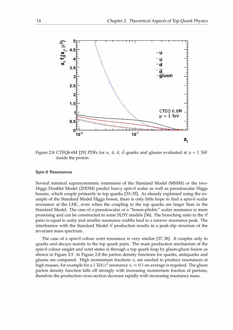
Figure 2.8: CTEQ6.6M [29] PDFs for u, u, d, d quarks and gluons evaluated at µ = 1 TeVinside the proton.
Spin-0 Resonances
Several minimal supersymmetric extensions of the Standard Model (MSSM) or the two-Higgs Doublet Model (2HDM) predict heavy spin-0 scalar as well as pseudoscalar Higgsbosons, which couple primarily to top quarks [33–35]. As already explained using the ex-ample of the Standard Model Higgs boson, there is only little hope to find a spin-0 scalarresonance at the LHC, even when the coupling to the top quarks are larger than in theStandard Model. The case of a pseudoscalar or a “boson-phobic” scalar resonance is morepromising and can be constructed in some SUSY models [36]. The branching ratio to the ttpairs is equal to unity and smaller resonance widths lead to a narrow resonance peak. Theinterference with the Standard Model tt production results in a peak-dip structure of theinvariant mass spectrum.
The case of a spin-0 colour octet resonance is very similar [37, 38]. It couples only toquarks and decays mainly to the top quark pairs. The main production mechanism of thespin-0 colour singlet and octet states is through a top quark loop by gluon-gluon fusion asshown in Figure 2.9. In Figure 2.8 the parton density functions for quarks, antiquarks andgluons are compared. High momentum fractions xi are needed to produce resonances athigh masses, for example for a 1 TeV/c2 resonance xi ≈ 0.1 on average is required. The gluonparton density function falls off strongly with increasing momentum fraction of partons,therefore the production cross section decrease rapidly with increasing resonance mass.

2.3 Top Quark Pair Production in the BSM Models 15
Spin-1 Resonances
Spin-1 colour singlet resonances will be produced via quark-antiquark annihilation asdrawn in Figure 2.9. It can be a excitation of a Standard Model gauge boson from some extradimensional model [39,40] or new gauge bosons which can arise in various electro-weak ex-tensions of the Standard Model [41–44]. Additional gauge symmetries can explain the massdifferences between the third family and the first two families as well as small quark CKMmixing matrix elements between the families. The family non-universal couplings generateflavour changing neutral currents, therefore these models are strongly constrained by theelectro-weak precision measurements at LEP.
Technicolor models [45] provide a dynamical approach to electro-weak and flavour sym-metry breaking. The new interactions are asymptotically free at very high energies andbecome strong and confining at lower energies. The masses of fermions and bosons aregenerated through dynamics of new interactions similar to the mass generation in QCD.Each Standard Model particle gets its corresponding techniparticle. Massive colour octetgauge bosons, colorons, mediate the interaction between fermions and technifermions andgenerate the fermion masses.
The Topcolor model [46] explains the large top quark mass through the formation of adynamical tt condensat, generated by a new strong force, which couples preferentially to thethird generation. The mediator of the new strong force is a neutral gauge boson, Z′, with anattractive interaction between tt and a repulsive interaction between bb to block the forma-tion of a bb condensate. Combination of these two theoretical models, the so-called “topcolorassisted technicolor” model [47] provides a dynamical mechanism for electro-weak symme-try breaking and explains the large top quark mass.
The Z′ boson decaying into top quark pairs produces a simple narrow peak in the in-variant mass spectrum. The width and the height of the peak depends on the strength ofthe couplings to the fermions. For massive colorons a coupling strength equal to the strongcoupling αS can be assumed for their coupling to quarks. Therefore the resonance peak willbe more pronounced than for a colour singlet Z′ boson.
Spin-2 Resonances
The interactions between gravitons and Standard Model particles are suppressed at TeV en-ergies, but there are some models with extra dimensions where the contributions from gravi-tons could be visible at the LHC. The Randall-Sundrum model [48, 49] postulates one extradimension that is compactified to a orbifold. Two branes exist on the orbifold, a “Plank”brane and a “TeV” brane where the Standard Model fields are confined. It predicts a limitednumber of Kaluza Klein modes but the couplings are enhanced by a large “warp” factor.The tt invariant mass spectrum is disturbed by a series of narrow width peaks.
A few benchmark models and corresponding parameters are listed in Table 2.2.

16 Chapter 2. Theoretical Aspects of Top Quark Physics
g
g
φ
t
t
q
q
Z′
t
t
Figure 2.9: Feynman diagrams for resonant tt production: spin-0 colour singlet or octet par-ticle φ and spin-1 Z′ boson resonance.
resonance spin colour mass, GeV/c2 σX × BR(X → tt), pb Γ/mX
SM Higgs 0 0 400 1.65 7%sequential Z′ 1 0 1000 1.6 2.7%topcolor Z′ 1 0 1000 6.6 3.3%graviton (k/MPl = 0.1) 2 0 1000 2.0 1.4%KK gluon 1 8 1000 27.8 15.3%
Table 2.2: Overview of some tt resonance benchmark models.
Experimental Constraints
New particles in the BSM theories are indirectly constrained by electro-weak data from LEPand directly by the searches at the TEVATRON. None of the searches at LEP or the TEVATRON
have led to an observation of a significant deviation from the Standard Model expectation.The results have been used to contrain the models. Di-lepton searches exclude sequentialZ′ boson with masses lower 1 TeV/c2 at 95% confidence level [50–52]. Di-jet searches leadto severe constraints on Z′ bosons, but constrain models involving coloured objects likeexcited quarks, axigluons, colorons stronger. The upper mass limit varies from 600 GeV/c2
to 1250 GeV/c2 depending on the model [53]. The tt searches have been primarily usedto constrain models, where the top quark acquires a special role. TEVATRON’s lower masslimit is around 820 GeV/c2 at 95% confidence level for a leptophobic Z′ boson in the Topcolormodel [54, 55]. Limits on couplings to fermions have been obtained for models predictingKaluza-Klein gluons, which do not couple to leptons and quarks of the third family arefavoured over light quarks [56–58].
Neutral Spin-1 Colour Singlet Z′ Boson
Additional U(1)′ gauge symmetries lead to the existence of neutral spin-1 colour singlet Z′
gauge bosons. The interaction of Z′ boson to the Standard Model fermions f can be writtenas [59]:
L =g
4 cos θWf γµ(CV − CAγ5) f Z′µ, (2.17)

2.3 Top Quark Pair Production in the BSM Models 17
where g = 0.626 is the SU(2)L gauge coupling, θW is the Weinberg angle and γµ, γ5 are thechiral operators. The axial CA and vector CV couplings to fermions can be expressed as:
CA = 2 cos θW(z fL − z fR)gZ′/g, (2.18)
CV = 2 cos θW(z fL + z fR)gZ′/g, (2.19)
with the U(1)Z′ gauge coupling gZ′ and the left and right handed fermion charges z fL andz fR . The couplings to fermions are free parameters and can be set for example the same as theStandard Model Z boson couplings. This so-called “sequential” Standard Model (SSM) isnot gauge invariant, but is often used for purpose of comparison and is representative for alarge range of models. The narrow width Z′ boson exclusion limits from pp and pp collisionsshow only a weak model dependence [60]. The Z′ boson production cross section dependson the fourth power of the model dependent couplings to fermions, but the properties of theparton density functions leads only to an effective logarithmic dependence on the couplingsas investigated in [61]. Thus, the SSM serves as a useful reference case.
At pp colliders only a direct production of Z′ boson via Drell-Yan process is allowed. Ingeneral the Drell-Yan production cross section is proportional to:
σ(qq→ Z′ → f f ) ∝s
(s−m2Z′)2 + sΓ2
Z′, (2.20)
where√
s is the partonic centre-of-mass energy of the process. In the limit of infinite centre-
of-mass energy the Drell-Yan production is preferred and the differential cross sectiondσZ′
dmZ′peaks at Z′ boson mass with the width of ΓZ′ . In the limit of infinite Z′ boson mass theshape will correspond to the f f continuum shape with the highest cross section at the f fmass threshold. At finite mZ′ and centre-of-mass energy, at the LHC 〈
√s〉 ∼ 600 GeV, we
have a mixture of both cases [62]. Figure 2.10 demonstrates how the tails to lower massesbecome more pronounced with increasing mZ′ .

18 Chapter 2. Theoretical Aspects of Top Quark Physics
]2 [GeV/cZ’m500 1000 1500 2000 2500 3000 3500
Eve
nt
Fra
ctio
n
-410
-310
-210
-110
no
rmal
ized
to
un
it a
rea
Figure 2.10: Z′ boson mass distributions for Z′ → tt in the mass range 500-3000 GeV/c2.
3 LHC and ATLAS Detector
The Large Hadron Collider (LHC) is a two-ring-superconducting hadron accelerator andcollider installed in a 26.7 km tunnel, that has been constructed between 1984 and 1989for the Large Electron Positron machine, LEP. It is designed to collide proton beams witha centre-of-mass energy of 14 TeV and a peak luminosity of 1034 cm−2s−1 as well as leadions with an energy of 2.8 TeV per nucleon and a peak luminosity of 1027 cm−2s−1. Thereare five main experiments acquiring LHC collision data. ATLAS [63] and CMS [64] are twogeneral purpose experiments aiming at the highest luminosity for proton operation. Thelow luminosity experiments are LHCb [65] for B-physics and TOTEM [66] for the detectionof protons from elastic scattering at small angles. ALICE [67] is a dedicated ion experimentfor the lead-lead ion operation. A brief summary of the accelerator and collider complex aswell as of the ATLAS detectors will be provided in this chapter. More detailed informationcan be found in the overviews about the LHC machine [68] and the ATLAS experiment [63].
3.1 The Large Hadron Collider
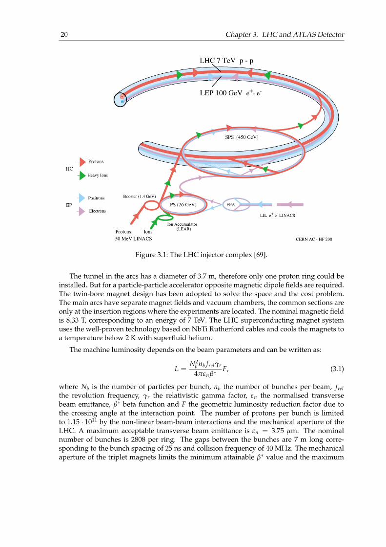
The injector chain Linac2 – Proton Synchrotron Booster (PSB) – Proton Synchrotron (PS) –Super Proton Synchrotron (SPS) supply the LHC rings with protons as illustrated in Figure3.1. The linear accelerator Linac2 with a length of 30 m (first run in 1978) provides pulsed1 Hz beams of up to 175 mA at 50 MeV, with pulse lengths varying between 20 and 150 µsdepending on the required number of protons. The beams are injected into the PSB, the firstand smallest circular proton accelerator. It was built in 1972 and contains four superimposedrings with a radius of 25 meters. The protons are accelerated up to 1.4 GeV and are fed tothe PS, a circular accelerator with a circumference of 628.3 m. It was built in the late 1950sand has been upgraded several times to improve the performance. The PS accelerates thebeams to 26 GeV and can produce bunch trains with the LHC bunch spacing of 25 ns, whichare then sent to SPS. It is a 6.9 km long circular accelerator and took its operation in 1976.It accelerates protons up to 450 GeV and injects protons in the LHC in a clockwise andanticlockwise direction. Finally the protons are accelerated to the nominal energy in theLHC rings, where they continue to circulate.
The LHC tunnel was designed for the electron-positron machine LEP. It has eight straightsections and eight arcs and lies between 45 m and 170 m below the surface on a plane in-clined at 1.4% sloping towards the Léman lake. The long straight sections were necessaryfor the LEP to reduce energy lost though the synchroton radiation. The LHC machine doesnot have the same synchrotron radiation problem like LEP, because protons are 104 timesheavier than electrons and the synchrotron radiation is proportional to 1/m4 of the particlemass m. Longer arcs and shorter straight sections would be ideal, but accepting the tunnel“as built” was the cost-effective solution.
20 Chapter 3. LHC and ATLAS Detector
Figure 3.1: The LHC injector complex [69].
The tunnel in the arcs has a diameter of 3.7 m, therefore only one proton ring could beinstalled. But for a particle-particle accelerator opposite magnetic dipole fields are required.The twin-bore magnet design has been adopted to solve the space and the cost problem.The main arcs have separate magnet fields and vacuum chambers, the common sections areonly at the insertion regions where the experiments are located. The nominal magnetic fieldis 8.33 T, corresponding to an energy of 7 TeV. The LHC superconducting magnet systemuses the well-proven technology based on NbTi Rutherford cables and cools the magnets toa temperature below 2 K with superfluid helium.
The machine luminosity depends on the beam parameters and can be written as:
L =N2
b nb frelγr
4πεnβ∗F, (3.1)
where Nb is the number of particles per bunch, nb the number of bunches per beam, frelthe revolution frequency, γr the relativistic gamma factor, εn the normalised transversebeam emittance, β∗ beta function and F the geometric luminosity reduction factor due tothe crossing angle at the interaction point. The number of protons per bunch is limitedto 1.15 · 1011 by the non-linear beam-beam interactions and the mechanical aperture of theLHC. A maximum acceptable transverse beam emittance is εn = 3.75 µm. The nominalnumber of bunches is 2808 per ring. The gaps between the bunches are 7 m long corre-sponding to the bunch spacing of 25 ns and collision frequency of 40 MHz. The mechanicalaperture of the triplet magnets limits the minimum attainable β∗ value and the maximum
3.2 The Atlas Detector 21
detector component required resolution η coveragemeasurement trigger
tracking σpT/pT = 0.05% pT ⊕ 1% ± 2.5 –
electromagneticσE/E = 10% /
√E ⊕ 0.7% ± 3.2 ± 2.5calorimetry
hadronic calorimetrybarrel and end-cap σE/E = 50% /
√E ⊕ 3% ± 3.2 ± 3.2
forward σE/E = 100% /√
E ⊕ 10% 3.1 < |η| < 4.9 3.1 < |η| < 4.9
muon spectrometer σpT /pT = 10% at pT = 1 TeV/c ± 2.7 ± 2.4
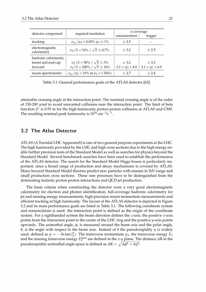
Table 3.1: General performance goals of the ATLAS detector [63].
attainable crossing angle at the interaction point. The nominal crossing angle is of the orderof 150-200 µrad to avoid unwanted collisions near the interaction point. The limit of betafunction β∗ is 0.55 m for the high-luminosity proton-proton collisions at ATLAS and CMS.The resulting nominal peak luminosity is 1034 cm−2s−1.
3.2 The Atlas Detector
ATLAS (A Toroidal LHC ApparatuS) is one of two general purpose experiments at the LHC.The high luminosity provided by the LHC and high cross sections due to the high energy en-able further precision tests of the Standard Model as well as searches for physics beyond theStandard Model. Several benchmark searches have been used to establish the performanceof the ATLAS detector. The search for the Standard Model Higgs boson is particularly im-portant, since a broad range of production and decay mechanisms is covered by ATLAS.Many beyond Standard Model theories predict new particles with masses in TeV-range andsmall production cross sections. These rare processes have to be distinguished from thedominating inelastic proton-proton interactions and QCD jet production.
The basis criteria when constructing the detector were a very good electromagneticcalorimetry for electron and photon identification, full-coverage hadronic calorimetry forjet and missing energy measurements, high-precision muon momentum measurements andefficient tracking at high luminosity. The layout of the ATLAS detector is depicted in Figure3.2 and its main performance goals are listed in Table 3.1. The following coordinate systemand nomenclature is used: the interaction point is defined as the origin of the coordinatesystem. For a righthanded system the beam direction defines the z-axis, the positive x-axispoints from the interaction point to the centre of the LHC ring and the positive y-axis pointsupwards. The azimuthal angle, φ, is measured around the beam axis and the polar angle,θ, is the angle with respect to the beam axis. Instead of θ the pseudorapidity η is widelyused, defined as η = − ln tan( θ
2 ). The transverse momentum pT, the transverse energy ETand the missing transverse energy Emiss
T are defined in the x-y plane. The distance ∆R in thepseudorapidity-azimuthal angle space is defined as ∆R =
√∆φ2 + ∆η2.

22 Chapter 3. LHC and ATLAS Detector
Figure 3.2: View of the ATLAS detector [70]. It measures 44m in length, has a diameter of25m and weighs about 7000 tons.
The detector is built forward-backward symmetric around the interaction point. Theinnermost part is a tracking detector. Measurements in the high-resolution semiconductorpixel and strips detectors are combined with the measurements in the straw-tube trackingdetector, that allows to distinguish particle types by the transition radiation. The trackingdetector is immersed in a 2 T solenoidal magnetic field. The high granularity liquid-argon(LAr) electromagnetic sampling calorimeters cover the pseudorapidity range |η| < 3.2. Thehadronic calorimeter in the range |η| < 1.7 is a scintillator-tile calorimeter, in the end-caps1.5 < |η| < 3.2 the LAr technology has been used. The LAr forward electromagnetic andhadronic calorimeters extend the pseudorapidity coverage to |η| = 4.9. The calorimeter issurrounded by the muon spectrometer consisting of three layers of high precision trackingchambers. One barrel and two end-caps of the large superconducting air-core toroid gener-ate the magnetic field in the spectrometer.
A short summary of most important properties of the ATLAS detector components willbe presented in the following sections.
Inner Detector
The inner detector is designed to measure tracks of charged particles above a given trans-verse momentum threshold (100 MeV/c in the initial measurements of minimum bias eventsand 500 GeV/c at high luminosities because of the increasing track multiplicity) and within

3.2 The Atlas Detector 23
the pseudorapidity range of |η| < 2.5. Precise measurements in the innermost pixel layer isone of the important requirements for a good b-jet identification and allows one to recon-struct secondary vertices a few millimetre distant from the interaction point. The detectoris contained within a cylindrical envelope of 3512 mm length and 1150 mm radius and iscomposed of three sub-elements. Figure 3.3 shows drawings of the sensors and structuresof the inner detector as well as the exact positions of the elements.
At innermost radii the pixel detector is placed containing of three silicon pixel layersin the barrel region and three silicon pixel discs in each of the end-caps. The layers arecomposed of 112 staves and the discs of 48 sectors, assembled on the supporting carbon-fibre structure. All staves and sectors are identical in the construction. 13 modules aremounted on each stave and 6 modules on each sector. The barrel modules are located in theway to have no gaps in the detector, this requires an overlap of the modules in z and φ. Thedisk modules are mounted on both sides of the disk, which are slightly twisted to achievethe complete coverage.
The barrel and disk modules are identical. The main components of a pixel module area silicon sensor, 16 electronic readout chips (FEs) 18x160 pixels each, a module controllerchip (MCC), and the interconnection foil (flex) as shown in Figure 3.4. The sensitive silicondetector area is connected via bump bonds with the front-end chips. The nominal pixel sizeis 50×400 µm2 (about 90% of pixels) and is defined by the read-out pitch of the front-endchips. The size of the remaining pixels is 50×600 µm2 in the regions between two front-end chips on a module to avoid dead space. The barrel pixels are assembled in the waythat 400 (600) µm are positioned along the z-axis and the disk pixels have 400 (600) µm inr, defined as
√x2 + y2. The detector typically provides three space points per track with a
resolution of about 10 µm in rφ and about 115 µm in z (or r in end-caps).
The pixel detector is surrounded by the SemiConductor Tracker (SCT), which consists offour concentric barrel layers in the radial range between 299 and 514 mm and nine disks inthe forward and backward region in the longitudinal range between 853.8 and 2720.2 mm.The SCT detector consists of 4088 modules, 2112 modules are installed in the barrel and 1976modules in the end-caps. The modules use 80 µm pitch micro-strip sensors, two each on thetop and bottom side rotated by± 20 mrad around the geometrical centre of the sensors. Theactive length of the barrel modules is 126.09 mm. In the inner end-caps the active length is59.1 mm, in the middle 115.61 mm (in the short-middle end-caps 52.48 mm) and in the outerend-caps 119.14 mm, see Figure 3.4. The dead space between sensors is 2.09 mm. The SCTprovides a space point resolution of about 17 µm in rφ and about 580 µm in z (or r in theend-caps).
The Transition Radiation Tracker (TRT) combines the concept of a straw tracker with thetransition radiation detection for the particle identification. It consists of 52 544 straws of144 cm in length in the barrel region and 319 488 straws of 37 cm in length arranged inwheels in both end-cap regions. Figure 3.5 presents the TRT barrel and end-caps structuresand modules. The straws have a diameter of 4 mm. The barrel consists of three cylindricalrings, each containing 32 modules. Each module contains axially positioned straws. Theend-caps consist of three wheels with radial positioned straws. All straws are embeddedin stacks of polypropylene/polyethylene fibres, which produce transition-radiation X-raysused for the particle identification. The straw anodes are 31 µm in diameter gold-plated
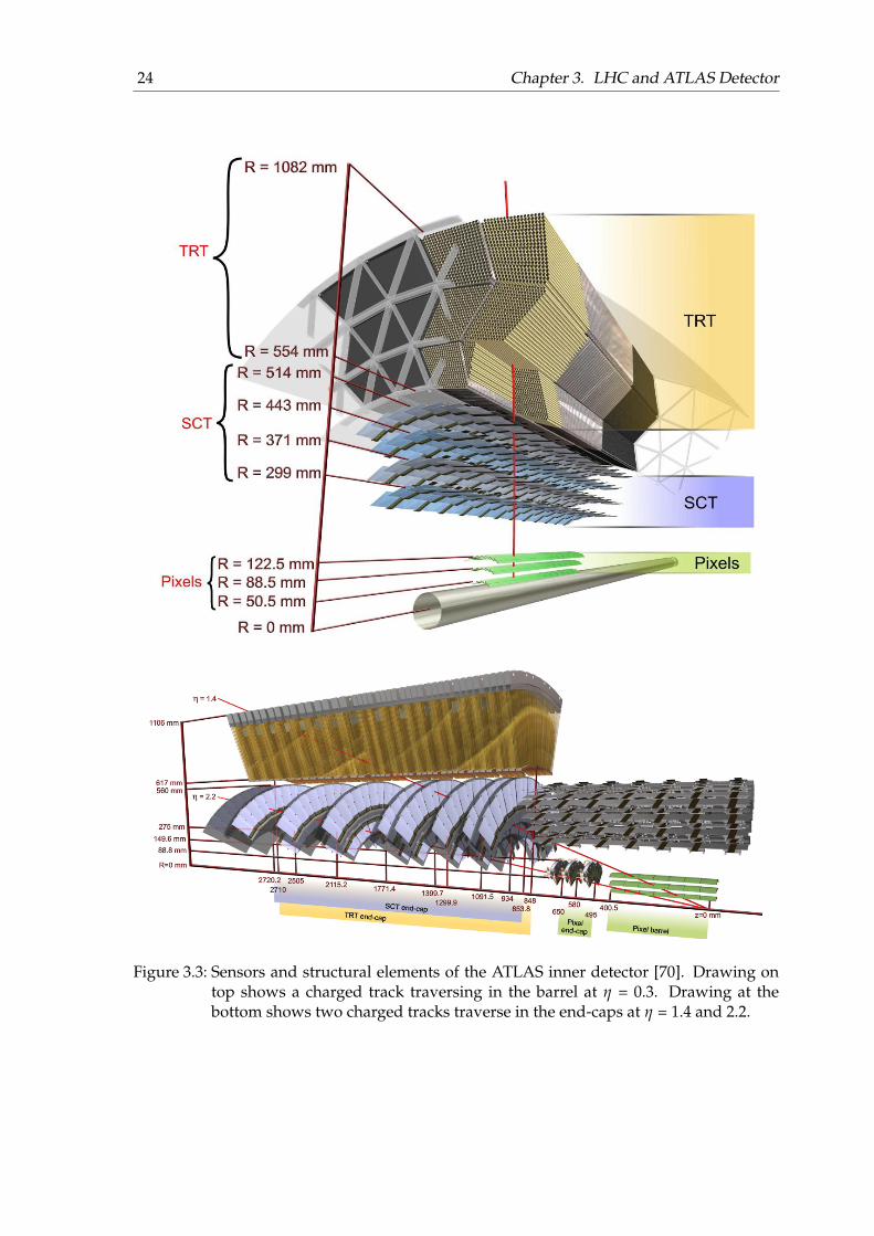
24 Chapter 3. LHC and ATLAS Detector
Figure 3.3: Sensors and structural elements of the ATLAS inner detector [70]. Drawing ontop shows a charged track traversing in the barrel at η = 0.3. Drawing at thebottom shows two charged tracks traverse in the end-caps at η = 1.4 and 2.2.

3.2 The Atlas Detector 25
(a) pixel barrel module (b) SCT end-cap modules
Figure 3.4: (a) Schematic view of a barrel pixel module and the SCT end-cap modules. (b)The upper photograph on the right shows the outer, middle and inner modules(from left to right). The lower schematic shows the components of the middlemodule [63].
Figure 3.5: (a) Photograph of one quarter of the barrel TRT. (b) The triangular design of thesupport structure and the shapes of the inner, middle and outer TRT modules canbe seen. Photograph of a TRT end-cap wheel (right) with 4 planes of straws [63].

26 Chapter 3. LHC and ATLAS Detector
Figure 3.6: Cut-away view of the calorimeter system [70].
tungsten wires. The ionisation gas is a xenon-base gas mixture (70% Xe, 23% CO2 and 3%O2). All charged tracks with pT > 500 MeV/c and |η| < 2 will traverse at least 36 straws,except in the barrel-end-caps transition region (0.8 < |η| < 1.0), where only 22 measurementsare possible. Typically seven to ten high threshold hits from transition radiation are expectedfor electrons above 2 GeV/c. The intrinsic straw rφ resolution is 130 µm, implying that eachwire position is constrained within ± 50 µm.
The high-radiation environment imposes stringent conditions on the inner-detector sen-sors, on-detector electronics, mechanical structure and services. To maintain an adequatenoise performance after radiation damage, the silicon sensors must be kept at low tempera-ture of approximately -15 °C. The TRT can be operated at room temperature.
Calorimeters
The ATLAS calorimeters consist of a number of sampling detectors with full φ-symmetryand coverage in η. The signal redout is separated from the particle absorption. Theschematic view of the components is shown in Figure 3.6 and its main parameters are listedin Table 3.2. The calorimeters closest to the beampipe are housed in cryostats. The barrelcryostat contains the electromagnetic calorimeter. The end-cap cryostats contain electromag-netic (EMEC) and hadronic (HEC) end-cap calorimeters and a forward hadronic calorime-
3.2 The Atlas Detector 27
barrel end-cap
electromagnetic calorimeter granularity ∆φ× ∆η versus η
presampler 0.025 × 0.1 |η| < 1.52 0.025 × 0.1 1.5 < |η| < 1.8
calorimeter 0.025/8 × 0.1 |η| < 1.40 0.050 × 0.1 1.375 < |η| < 1.4251st layer 0.025 × 0.025 1.40 < |η| < 1.475 0.025 × 0.1 1.425 < |η| < 1.5
0.025/8 × 0.1 1.5 < |η| < 1.80.025/6 × 0.1 1.8 < |η| < 2.00.025/4 × 0.1 2.0 < |η| < 2.40.025 × 0.1 2.4 < |η| < 2.50.1 × 0.1 2.5 < |η| < 3.2
calorimeter 0.025 × 0.025 |η| < 1.40 0.050 × 0.025 1.375 < |η| < 1.4252nd layer 0.075 × 0.025 1.40 < |η| < 1.475 0.025 × 0.025 1.425 < |η| < 2.5
0.1 × 0.1 2.5 < |η| < 3.2
calorimeter 0.050 × 0.025 |η| < 1.35 0.050 × 0.025 1.5 < |η| < 2.53rd layer
Number of readout channels
presampler 7808 1536 (both sides)calorimeter 101760 62208 (both sides)
LAr hadronic end-cap calorimeter granularity ∆φ× ∆η versus η
0.1 × 0.1 1.5 < |η| < 2.50.2 × 0.2 2.5 < |η| < 3.2
LAr hadronic forward calorimeter granularity ∆x× ∆y (cm) versus η
FCal1: 3.0 × 2.6 3.15 < |η| < 4.30FCal1: 3.10 < |η| < 3.15∼ four times finer 4.30 < |η| < 4.83FCal2: 3.3 × 4.2 3.24 < |η| < 4.50FCal2: 3.20 < |η| < 3.24∼four times finer 4.50 < |η| < 4.81FCal3: 5.4 × 4.7 3.32 < |η| < 4.60FCal3: 3.29 < |η| < 3.32∼ four times finer 4.60 < |η| < 4.75
Scintillator tile calorimeter granularity ∆φ× ∆η
1st, 2nd layer 0.1 × 0.1 0.1 × 0.1 (extended barrel)3rd layer 0.2 × 0.1 0.2 × 0.1 (extended barrel)
Number of readout channels
LAr end-cap 5632 (both sides)LAr forward 3524 (both sides)
scintillator tile 5760 4092 (both sides, extended barrel)
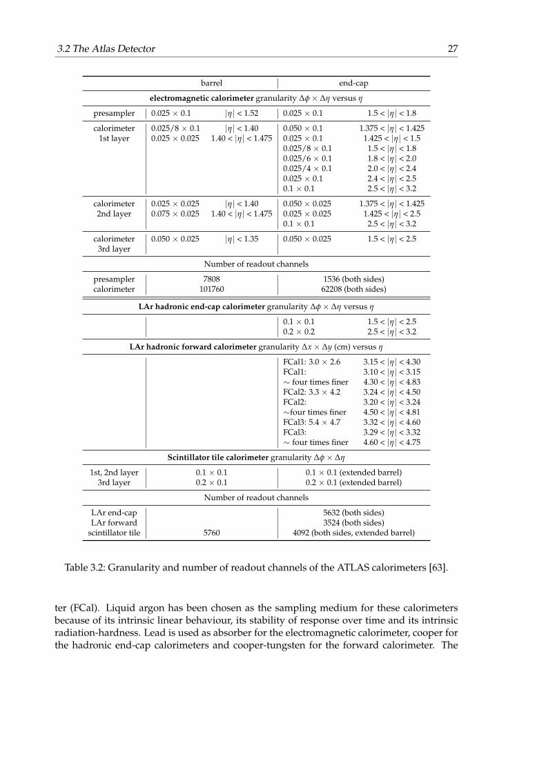
Table 3.2: Granularity and number of readout channels of the ATLAS calorimeters [63].
ter (FCal). Liquid argon has been chosen as the sampling medium for these calorimetersbecause of its intrinsic linear behaviour, its stability of response over time and its intrinsicradiation-hardness. Lead is used as absorber for the electromagnetic calorimeter, cooper forthe hadronic end-cap calorimeters and cooper-tungsten for the forward calorimeter. The
28 Chapter 3. LHC and ATLAS Detector
∆ϕ = 0.0245
∆η = 0.02537.5mm/8 = 4.69 mm ∆η = 0.0031
∆ϕ=0.0245x4 36.8mmx4 =147.3mm
Trigger Tower
TriggerTower∆ϕ = 0.0982
∆η = 0.1
16X0
4.3X0
2X015
00 m
m
470 m
m
η
ϕ
η = 0
Strip cells in Layer 1
Square cells in Layer 2
1.7X0
Cells in Layer 3 ∆ϕ×∆η = 0.0245×0.05
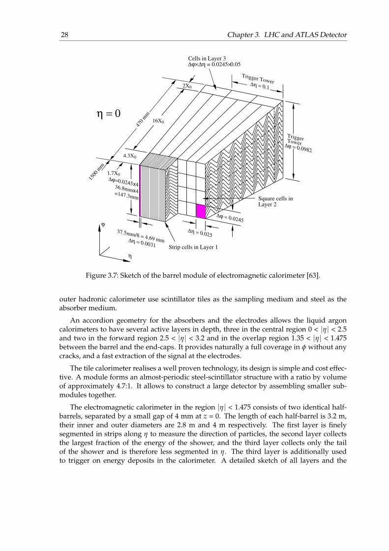
Figure 3.7: Sketch of the barrel module of electromagnetic calorimeter [63].
outer hadronic calorimeter use scintillator tiles as the sampling medium and steel as theabsorber medium.
An accordion geometry for the absorbers and the electrodes allows the liquid argoncalorimeters to have several active layers in depth, three in the central region 0 < |η| < 2.5and two in the forward region 2.5 < |η| < 3.2 and in the overlap region 1.35 < |η| < 1.475between the barrel and the end-caps. It provides naturally a full coverage in φ without anycracks, and a fast extraction of the signal at the electrodes.
The tile calorimeter realises a well proven technology, its design is simple and cost effec-tive. A module forms an almost-periodic steel-scintillator structure with a ratio by volumeof approximately 4.7:1. It allows to construct a large detector by assembling smaller sub-modules together.
The electromagnetic calorimeter in the region |η| < 1.475 consists of two identical half-barrels, separated by a small gap of 4 mm at z = 0. The length of each half-barrel is 3.2 m,their inner and outer diameters are 2.8 m and 4 m respectively. The first layer is finelysegmented in strips along η to measure the direction of particles, the second layer collectsthe largest fraction of the energy of the shower, and the third layer collects only the tailof the shower and is therefore less segmented in η. The third layer is additionally usedto trigger on energy deposits in the calorimeter. A detailed sketch of all layers and the

3.2 The Atlas Detector 29
granularity in η and φ is presented in Figure 3.7. To measure the energy lost by electronsand photons before reaching the calorimeter, a presampler detector is placed in front ofthe barrel. It is a thin liquid argon layer with 11 mm in depth. The electromagnetic end-cap calorimeters consist of two wheels covering the range 1.375 < |η| < 3.2. Each wheelis 63 cm thick, the external and internal radii are 2098 mm and 330 mm, respectively. Inthe overlap region between the barrel and the end-cap calorimeters, where the material infront of the calorimeter amounts to several interaction lengths, again a LAr presampler isinstalled, covering the range 1.5 < |η| < 1.8. The resolution of the electromagnetic calorimeteris expected to be σE/E = 10%/
√E⊕ 0.7%.
The hadronic tile calorimeter is located in the region, |η| < 1.7, behind the electromag-netic calorimeter. It is comprised of a central barrel, 5.8 m in length, and two extendedbarrels, 2.6 m in length and each having an inner radius of 2.28 m and an outer radius of4.25 m. The barrels are divided azimuthally into 64 modules and are segmented in depthin three layers. The hadronic end-cap calorimeter covers the range 1.5 < |η| < 3.2, overlap-ping with the tile and forward calorimeters to reduce the drop in material density in thetransition region. The hadronic end-cap calorimeter consists of two wheels per end-cap and32 identical modules per wheel. Each wheel is divided into two segments in depth, for atotal of four layers per end-cap. The wheels closest to the interaction point are built from25 mm parallel copper plates, while those further away use 50 mm copper plates. The cop-per plates are interleaved with 8.5 mm LAr gaps. The outer radius of the copper plates is2.03 m, while the inner radius is 0.475 m. Except in the overlap region with the forwardcalorimeter where this radius becomes 0.372 m. The forward calorimeter located in the re-gion 3.1 < |η| < 4.9 consists of three modules in each end-cap. The first module is made ofcooper and optimised for electromagnetic measurements. The other two layers are made oftungsten and measure predominantly the energy of hadronic interactions. The resolutionof the hadronic calorimeters is expected to be σE/E = 50% /
√E ⊕ 3% in the barrel and
end-caps and σE/E = 100%/√
E⊕ 10% in the forward calorimeter.
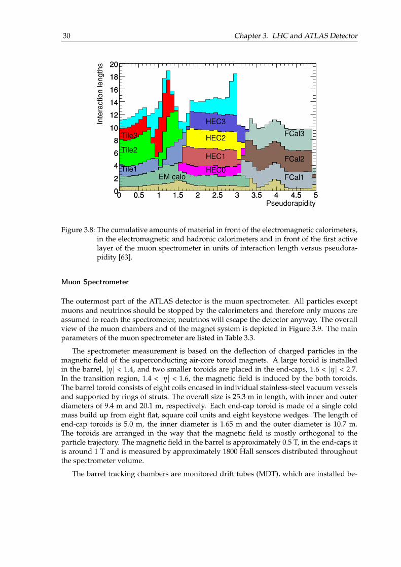
The total thickness of the electromagnetic calorimeter is more than 24 radiation lengthsin the barrel and above 26 radiation lengths in the end-caps. The total thickness of thehadronic calorimeter is approximately 9.7 interaction lengths in the barrel and 10 interactionlengths in the end-caps. The cumulative amounts of material in front of the electromagneticcalorimeters, in the electromagnetic and hadronic calorimeters and in front of the first activelayer of the muon spectrometer in units of interaction length is visible in Figure 3.8. Itprovides a good containment for electromagnetic and hadronic showers and limits punch-through of particles into the muon system.
On the inner face of the endcap calorimeter cryostats at z = ±3560 mm and perpendicu-lar to the beam direction the Minimum Bias Trigger Scintillators (MBTS) are mounted. Theywill be used to trigger on minimum collision activity for the initial running period at lumi-nosities below 1033 cm−2s−1. The MBTS detector consists of 32 scintillator paddles, 2 cmthick, organized into 2 disks, one on each side of the interaction point of ATLAS. The lightemitted by each scintillator segment is collected by wavelength-shifting optical fibers andguided to a photomultiplier tube. The signals are read out by the tile calorimeter electronics.
30 Chapter 3. LHC and ATLAS Detector
0 0.5 1 1.5 2 2.5 3 3.5 4 4.5 502468
101214161820
Pseudorapidity0 0.5 1 1.5 2 2.5 3 3.5 4 4.5 5
Inte
ract
ion
leng
ths
02468
101214161820
EM caloTile1
Tile2
Tile3
HEC0HEC1
HEC2
HEC3
FCal1
FCal2
FCal3
Figure 3.8: The cumulative amounts of material in front of the electromagnetic calorimeters,in the electromagnetic and hadronic calorimeters and in front of the first activelayer of the muon spectrometer in units of interaction length versus pseudora-pidity [63].
Muon Spectrometer
The outermost part of the ATLAS detector is the muon spectrometer. All particles exceptmuons and neutrinos should be stopped by the calorimeters and therefore only muons areassumed to reach the spectrometer, neutrinos will escape the detector anyway. The overallview of the muon chambers and of the magnet system is depicted in Figure 3.9. The mainparameters of the muon spectrometer are listed in Table 3.3.
The spectrometer measurement is based on the deflection of charged particles in themagnetic field of the superconducting air-core toroid magnets. A large toroid is installedin the barrel, |η| < 1.4, and two smaller toroids are placed in the end-caps, 1.6 < |η| < 2.7.In the transition region, 1.4 < |η| < 1.6, the magnetic field is induced by the both toroids.The barrel toroid consists of eight coils encased in individual stainless-steel vacuum vesselsand supported by rings of struts. The overall size is 25.3 m in length, with inner and outerdiameters of 9.4 m and 20.1 m, respectively. Each end-cap toroid is made of a single coldmass build up from eight flat, square coil units and eight keystone wedges. The length ofend-cap toroids is 5.0 m, the inner diameter is 1.65 m and the outer diameter is 10.7 m.The toroids are arranged in the way that the magnetic field is mostly orthogonal to theparticle trajectory. The magnetic field in the barrel is approximately 0.5 T, in the end-caps itis around 1 T and is measured by approximately 1800 Hall sensors distributed throughoutthe spectrometer volume.
The barrel tracking chambers are monitored drift tubes (MDT), which are installed be-

3.2 The Atlas Detector 31
Figure 3.9: Schematic view of the muon spectrometer [70].
tween and on the eight coils of the barrel magnet. They are arranged in three concentriccylindrical shells at radii of approximately 5 m, 7.5 m and 10 m from the beam axis. Due toa high particle flux in the transition region and in the end-caps the cathode strip chambers(CSC) have been installed in the innermost ring additionally to the three layers of MDTs. TheCSCs have a higher rate capability and time resolution than MDTs. The end-cap chambersare mounted in front and behind the end-cap toroids. They form large wheels, perpendic-ular to the z-axis and located at distances of |z| ∼ 7.4 m, 10.8 m, 14 m and 21.5 m from theinteraction point.
The MDTs are built of aluminum tubes of 30 mm diameter filled with argon-gas-mixtureat an absolute pressure of 3 bar and contain a 50 µm diameter tungsten-rhenium wire in thecentre. The typical single wire resolution is 80 µm, the resolution per chamber is 35 µm inthe bending plane. The CSCs are multi-wire proportional chambers filled with argon (30%) -carbonic acid (50%) - tetrafluormethane (20%) gas mixture with cathode planes segmentedinto strips in orthogonal directions. The diameter of one single wire made of tungsten-rhenium is 30 µm, its spatial resolution is about 60 µm. The resolution of a chamber is40 µm in the bending plane and about 5 mm in the transverse plane.
An essential design criterion of the muon system was the capability to trigger on muon
32 Chapter 3. LHC and ATLAS Detector
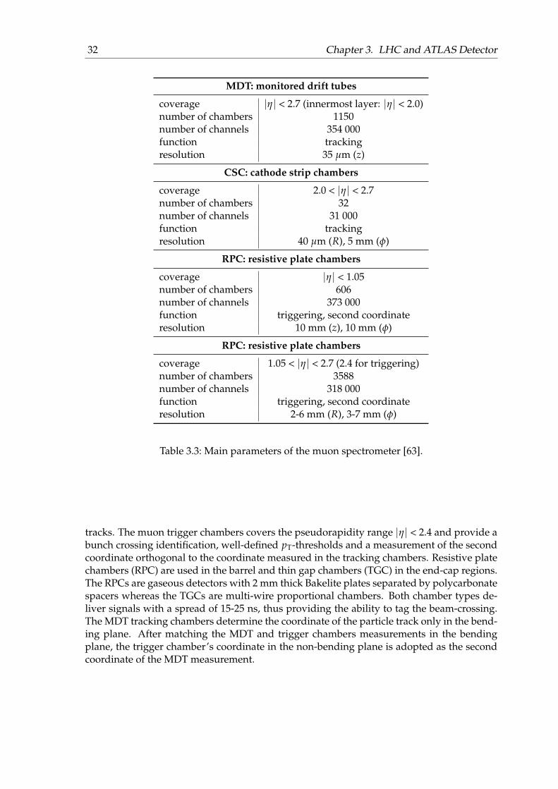
MDT: monitored drift tubes
coverage |η| < 2.7 (innermost layer: |η| < 2.0)number of chambers 1150number of channels 354 000function trackingresolution 35 µm (z)
CSC: cathode strip chambers
coverage 2.0 < |η| < 2.7number of chambers 32number of channels 31 000function trackingresolution 40 µm (R), 5 mm (φ)
RPC: resistive plate chambers
coverage |η| < 1.05number of chambers 606number of channels 373 000function triggering, second coordinateresolution 10 mm (z), 10 mm (φ)
RPC: resistive plate chambers
coverage 1.05 < |η| < 2.7 (2.4 for triggering)number of chambers 3588number of channels 318 000function triggering, second coordinateresolution 2-6 mm (R), 3-7 mm (φ)
Table 3.3: Main parameters of the muon spectrometer [63].
tracks. The muon trigger chambers covers the pseudorapidity range |η| < 2.4 and provide abunch crossing identification, well-defined pT-thresholds and a measurement of the secondcoordinate orthogonal to the coordinate measured in the tracking chambers. Resistive platechambers (RPC) are used in the barrel and thin gap chambers (TGC) in the end-cap regions.The RPCs are gaseous detectors with 2 mm thick Bakelite plates separated by polycarbonatespacers whereas the TGCs are multi-wire proportional chambers. Both chamber types de-liver signals with a spread of 15-25 ns, thus providing the ability to tag the beam-crossing.The MDT tracking chambers determine the coordinate of the particle track only in the bend-ing plane. After matching the MDT and trigger chambers measurements in the bendingplane, the trigger chamber’s coordinate in the non-bending plane is adopted as the secondcoordinate of the MDT measurement.
3.3 Forward Detectors 33
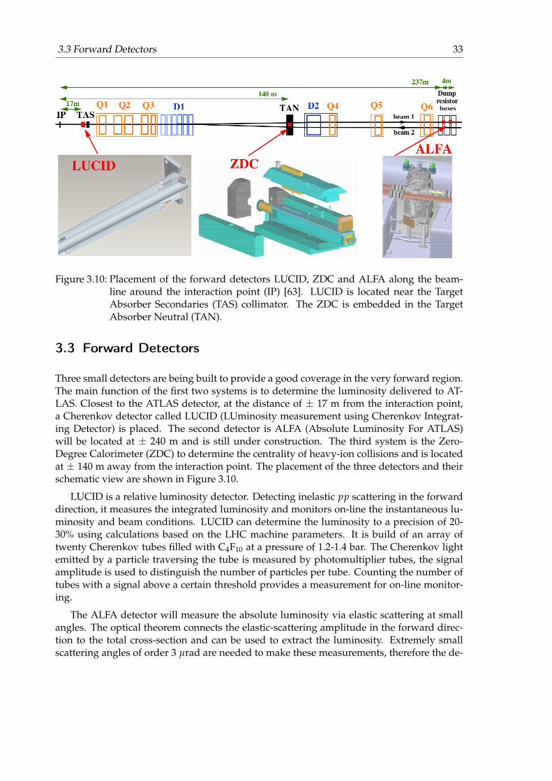
Figure 3.10: Placement of the forward detectors LUCID, ZDC and ALFA along the beam-line around the interaction point (IP) [63]. LUCID is located near the TargetAbsorber Secondaries (TAS) collimator. The ZDC is embedded in the TargetAbsorber Neutral (TAN).
3.3 Forward Detectors
Three small detectors are being built to provide a good coverage in the very forward region.The main function of the first two systems is to determine the luminosity delivered to AT-LAS. Closest to the ATLAS detector, at the distance of ± 17 m from the interaction point,a Cherenkov detector called LUCID (LUminosity measurement using Cherenkov Integrat-ing Detector) is placed. The second detector is ALFA (Absolute Luminosity For ATLAS)will be located at ± 240 m and is still under construction. The third system is the Zero-Degree Calorimeter (ZDC) to determine the centrality of heavy-ion collisions and is locatedat ± 140 m away from the interaction point. The placement of the three detectors and theirschematic view are shown in Figure 3.10.
LUCID is a relative luminosity detector. Detecting inelastic pp scattering in the forwarddirection, it measures the integrated luminosity and monitors on-line the instantaneous lu-minosity and beam conditions. LUCID can determine the luminosity to a precision of 20-30% using calculations based on the LHC machine parameters. It is build of an array oftwenty Cherenkov tubes filled with C4F10 at a pressure of 1.2-1.4 bar. The Cherenkov lightemitted by a particle traversing the tube is measured by photomultiplier tubes, the signalamplitude is used to distinguish the number of particles per tube. Counting the number oftubes with a signal above a certain threshold provides a measurement for on-line monitor-ing.
The ALFA detector will measure the absolute luminosity via elastic scattering at smallangles. The optical theorem connects the elastic-scattering amplitude in the forward direc-tion to the total cross-section and can be used to extract the luminosity. Extremely smallscattering angles of order 3 µrad are needed to make these measurements, therefore the de-
34 Chapter 3. LHC and ATLAS Detector
tectors have to be placed far away from the interaction point and as close as possible to thebeam. The Roman pots technique will be used to move the the scintillating-fibre tracker asclose as 1 mm to the beam. The goal is to measure the luminosity with an uncertainty ofbetter than 5%.
The primary purpose of ZDC is to detect forward neutrons in heavy-ion collisions andto measure the centrality of such collisions. During the start-up phase of the LHC it willenhance the acceptance of the ATLAS detector for diffractive processes and can also providean additional minimum-bias trigger for ATLAS.
3.4 Data Acquisition System
At the LHC the collision rate is 40 MHz for a bunch spacing of 25 ns. The LHC has startedits operation with a peak luminosity of 1029 cm−2s−1 and the luminosity will be increasedup to the design luminosity of 1034 cm−2s−1 step by step. The incoming interaction rate atthe design luminosity is about 1 GHz. On the one hand recording all data with such a highfrequency exceeds our technical possibilities and on the other hand we do not need to recordall physics processes with the same rate. Events with a lower production rate should berecorded more often than events with a higher production rate. The trigger system classifiesthe events by the specified properties and decides if a specific event will be written to massstorage or not.
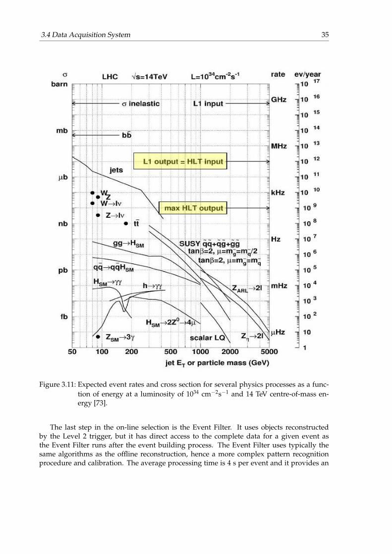
The ATLAS trigger system is based on three levels of event selection, which reduces theoutput event storage from 40 MHz rate to about 200 Hz rate. The first step is a hardwarebased Level 1 trigger [71]. The next two steps are software based Level 2 and Event Filtertriggers, collectively named as the High Level Trigger [72]. From Figure 3.11 we can see thereduction rates after each trigger level and production rates for different physics processes.The aim is to reduce the amount of low energy QCD processes and to achieve an efficientselection of rare processes.
The Level 1 trigger receives all collision data and has to take its decision within 2.5 µsto reduce the output rate to 75 kHz. The decision is based on the multiplicities and energythresholds for the following objects reconstructed by the Level 1 trigger algorithms: elec-tromagnetic clusters, taus, jets, missing transverse energy, scalar sum of transverse energyin the calorimeter, total transverse energy of observed jets and trajectories of muons mea-sured in the muon spectrometer. The total number of allowed Level 1 configurations is 256.Using a prescale factor N (where only 1 of N events is selected), each configuration can beweighted also depending on the current peak luminosity during the run.
The Level 2 trigger uses the regions-of-interest identified by the Level 1 trigger and anal-yses locally but using fine-grained data from the detector. Depending on the type of selectedobject the size of the region-of-interest is defined and the Level 1 object is re-reconstructedwith improved precision. The Level 2 trigger uses information from the inner detector,which is not available for the Level 1 trigger and combines information from different sub-detectors to provide additional purity of the selected events. The average processing time is40 ms, including the time for data transfers. The output rate is reduced to 2 kHz.
3.4 Data Acquisition System 35
Figure 3.11: Expected event rates and cross section for several physics processes as a func-tion of energy at a luminosity of 1034 cm−2s−1 and 14 TeV centre-of-mass en-ergy [73].
The last step in the on-line selection is the Event Filter. It uses objects reconstructedby the Level 2 trigger, but it has direct access to the complete data for a given event asthe Event Filter runs after the event building process. The Event Filter uses typically thesame algorithms as the offline reconstruction, hence a more complex pattern recognitionprocedure and calibration. The average processing time is 4 s per event and it provides an

36 Chapter 3. LHC and ATLAS Detector
additional rejection to 200 Hz.
The raw data events are written in one or more inclusive streams depending on the trig-ger decision. The initial streams are “egamma”, “jetTauEtmiss”, “muons”, and “minbias”.Each stream contains events that pass at least one of the trigger signatures. For example,events passing the electron or photon triggers will be written to the egamma stream. Thestreams have approximately the same proportion of events and the event duplication acrossstreams is less than 10%.
At the LHC start-up the strategy is to commission the trigger and the detector with well-measured Standard Model processes. Many triggers will operate in pass-through mode tovalidate the trigger selection and trigger reconstruction algorithms. With increasing lumi-nosity a higher thresholds and tighter selections will be applied to select the most interestingphysics processes.
3.5 Performance of the LHC and the ATLAS Experiment
In December 2009 the ATLAS detector has started to record data from collisions. The beamenergy and the corresponding dipole field is reduced to 3.5 TeV per beam to allow a safe op-eration. All main components of the detector are fully operational and all levels of the triggerand data aquisition system performed as expected. The approximate operational fraction ofATLAS detector components is listed in Table 3.4. The commissioning and calibration ofthe ATLAS detector was started during the cosmic ray data taking in 2008 and 2009. Per-formance close to design goals has been obtained for different detector components: innerdetector [74], LAr calorimeter [75] and muon spectrometer [76]. Currently collision dataat 7 TeV centre-of-mass energy is used to calibrate the detector as well for the first physicsstudies.
The instantaneous luminosity given by Equation 3.1 characterises the performance ofthe LHC machine. It is determined in real time approximately one per second using a num-ber of detectors and algorithms. The highest peak luminosity obtained to date is of order1032 cm−2s−1. The full history is displayed in Figure 3.13(a).
Integrating the instantaneous luminosity over time gives the integrated luminosity Lint,which corresponds to the amount of collected data. Figure 3.13(b) shows the delivered lu-minosity by the LHC machine and the recorded luminosity by the ATLAS experiment. Theuncertainty on the measured luminosity is 11% and has been obtained using an absolutecalibration via beam separation scans [77]. To calculate the number of events N of a certainphysics process, the total luminosity has to be multiplied with the probability of the processoccurring, the cross section σ:
N = σ · Lint (3.2)
The cross section σ given in cm 2 is preferably quoted in picobarn (pb), where 1 pb =10−36 cm2.

3.5 Performance of the LHC and the ATLAS Experiment 37
component num. of channels operational fraction
pixels 80 · 106 97.4%silicon strips 6.3 · 106 99.2%transition radiation tracker 350 · 103 98.0%LAr EM calorimeter 170 · 103 98.5%tile calorimeter 9800 97.3%hadronic endcap LAr calorimeter 5600 99.9%forward LAr calorimeter 3500 100%level 1 calo trigger 7160 99.9%level 1 muon RPC trigger 370 · 103 99.5%level 1 muon TGC trigger 320 · 103 100%muon drift tubes 350 · 103 99.7%cathode strip chambers 31 · 103 98.5%RPC barrel muon chambers 370 · 103 97.0%TGC endcap muon chambers 320 · 103 98.6%
Table 3.4: Operational fraction of ATLAS detector components (May, 2010).
Figure 3.12: (a) The delivered instantaneous luminosity measured online and taken at√
s =7 TeV. (b) The delivered and recorded by ATLAS total integrated luminosity at√
s = 7 TeV.

38 Chapter 3. LHC and ATLAS Detector
4 Event Simulation
The simulation of physics processes with the according detector response is an essential toolin high energy physics. During the preparation stage of a experiment it allows to predict sen-sitivity to various physics processes, to develop and to validate readout and reconstructionalgorithms. At the running stage of a experiment it is used to test predictions of theoret-ical models against the real detector response. The simulation is divided into three steps:generation of events and immediate decays, simulation of interactions in the detector anddigitalisation of energy deposited in the detector into voltages and currents for readout elec-tronics. The output format of the simulation is identical to the true detector output formatand can be run through the same trigger and reconstruction algorithms.
The first part of this chapter deals with simulation of physics processes. The main as-pects of the event generation techniques and the event generators used in this thesis will bediscussed. The second part summarise the simulation of detector response, the full detectorsimulation based on GEANT4 [78] and the fast detector simulation ATLFAST-II [79]. After-wards the simulated signal and background processes will the described in more details.
4.1 Main Aspects of Monte Carlo Event Simulation
The Monte Carlo event simulation enables the description of the final states resulting fromhigh-energy collisions. The state-of-the-art knowledge about quantum chromodynamicsis implemented using numerical Monte Carlo techniques. The aim is to produce eventsimitating Nature’s behaviour in a real experiment. The ability to isolate independent phasesof the overall collision, the concept of “factorisation”, makes possible to simulate complexfinal states with hundreds of particles.
In particular, factorisation allows to separate parts that describe the structure of the pro-ton and the final-state hadron formation from the hard interaction part. The time scale atthat the hard scattering takes place is so short, that the details of the parton distributionsand their interactions in proton or what will happen to it after the hard collision, are ir-relevant. Figure 4.1 illustrates the general structure of a hard proton-proton collision. Thehard interaction among the partons can be calculated perturbatively. The parton densityfunctions depend only on the energy scale of the hard scatterers and not on the nature ofthe probe and are determined by global fits to data from deep inelastic scattering, Drell-Yan and jet production. After the hard process, created partons emit themselves partons.The parton shower process, governed by perturbative QCD, continue until a low virtualityscale is reached (the region labelled with the dotted line in the figure). At this point thehadronisation process starts. The hadronisation is assumed to be independent of the initialhard process, therefore its parametrisation, tuned in some reference process, can be used in

40 Chapter 4. Event Simulation
Figure 4.1: General structure of a hard proton-proton collision [80].
other hard interactions. Nearby partons combine into colour-singlet clusters (the grey smallblobs in figure), which build hadrons. The remnants of colliding protons undergo similarshower and hadronisation processes. The evolution of the underlying event (the labelledlarge grey blob) depends on the hard event, because at least colour quantum numbers mustbe exchanged to guarantee overall neutralisation. In our picture, the initial partons emitfurther partons, which split into qq pairs shared with underlying event. Finally the decaysof unstable hadrons are handled. Multi-parton interactions, wherein more than one pair ofpartons from protons interact as well as pile-up from other proton-proton collisions in thesame bunch crossing are accounted for.
Additional partons in the final states can be handled in two ways: by the matrix elementor by the patron shower methods. In the matrix element method additional Feynman dia-grams are calculated, taking into account exact kinematics, interferences and helicity struc-ture. This approach is correct, but calculations becomes extensive with increasing numberof final states. The parton shower method allows to add an arbitrary number of branch-ings of one parton into two (or more) partons. It is possible by simplifying the kinematics,and the interference and helicity structure of the process. Both approaches have strong andweak points. The parton shower method yields good descriptions of relatively soft gluonemission, while at higher energy scale the matrix element method provides more reasonableresults. The ultimate goal is to combine the best aspects of the both methods.
There are multi-purpose Monte Carlo generators, which handle all phases of event sim-ulation, as well the specialised generators, which cover only single steps. The most accuratetheoretical predictions are often obtained by combining components of different simulationprograms - one program to produce a hard process, another to evolve the final states of the

4.1 Main Aspects of Monte Carlo Event Simulation 41
hard process through the parton shower, a third to hadronise the products of parton showerand so forth. Depending on the problem of interest, best suitable tools should be chosen.
In the following the used Monte Carlo programs and some simulation components willbe discussed in more details in context of their implementation in event generators.
4.1.1 Parton Level Event Generators
The parton level Monte Carlo event generators simulate final states consisting of leptons,bare quarks and gluons. The colliding partons can be considered as free at smallest scale intime and distance and the perturbative expansion provides reliable predictions. The code isoften based on the direct computation of the relevant Feynman diagrams, but also programsfor automatic generation of parton-level processes exist. At the tree level the limiting factorfor the automatic generation is the CPU power. The computation of higher order correctionsin particular of virtual emissions is technically more complex.
The parton-level computation has to be combined with the partonic evolution given bythe shower Monte Carlo programs in a consistent way. A final state with n partons canbe obtained from n− k partons generated by the matrix event generator plus k additionalpartons from the shower Monte Carlo simulations. This implies that the same final statecan be generated starting from different (n− k)-parton configurations. To avoid doublecounting the parton configuration generated by the parton shower should be matched tothe parton configuration generated by the matrix element generators.
ALPGEN
ALPGEN [81] allows exact computation of tree level matrix elements with a fixed number ofpartons in the final state for a large list of pre-defined Standard Model processes in hadroniccollisions. Emphasis has been placed on final states with a large parton multiplicity. Theb-quark and top quark masses are included, the c-quark mass is taken into account in somespecial cases and the top-quark and gauge-boson decays are implemented with helicity cor-relations. Full information on the colour and flavour structure of parton level events is pro-vided to enable the evolution of the partonic final states into fully hadronised final states. Astrategy [82, 83] has been developed to match the multiparton final states with the showerdevelopment. The phase space is separated in the matrix element and parton shower do-mains by definition of a cut value. The matrix elements are reweighted with Sudakov formfactors [84] and the parton showers are subjected to a veto procedure to cancel dependenceon the cut value to next-to-leading logarithmic accuracy.
MC@NLO
MC@NLO [85] is a method for matching next-to-leading order QCD calculations of hardprocesses and parton shower Monte Carlo simulations. The total rates are accurate to thenext-to-leading order, the distributions are recovered upon expansion in the strong cou-pling constant αS. The next-to-leading order calculations include virtual and real emissionof partons. The real emissions are also included in the parton shower simulation and this
42 Chapter 4. Event Simulation
should not be double-counted. The matching is based on the subtraction method widelyused for the next-to-leading order calculations. The result is a set of leading order and next-to-leading order parton configurations that are fed into a parton shower generator. In orderto reproduce the next-to-leading order corrections fully, some of the configurations havenegative weights. The MC@NLO formalism is general, but in the current version only theshowering and hadronisation code of HERWIG is supported.
4.1.2 Multi-purpose Event Generators
Multi-purpose event generators are able to simulate a wide variety of the initial and finalstates with the frequency as predicted by theory. The hard subprocess is often the onlyprocess dependent part and everything else is almost completely generic. Therefore suchgenerators have a modular structure and the parton level event generators can be interfacedto the shower and hadronisation modules. The multi-purpose simulation programs providean exclusive description of events. For example, a Z boson produced in the hard subprocesshas zero transverse momentum. Through the parton shower the transverse momentum canbe produced, since the final state particles from the hard subprocess must recoil againstthose produced by the shower. Thus, the general purpose generators are ideal to describethe full event necessary for a more realistic description of collision events.
PYTHIA
PYTHIA [86] is a general-purpose Monte Carlo program for hadronic event simulation inpp, e+e−and ep colliders. Around 300 different 2 → n (maximal 3) subprocesses are im-plemented. Not all contributing Feynman graphs are always included, but the more im-portant. Also various approximations in the matrix element calculations are used. To thepartonic processes the initial and final state parton shower are added. The final state showeris based on forward evolution in terms of decreasing time-like virtuality m2 = E2 − ~p2 withangular ordering imposed by veto. The framework is a leading-log approximation, but in-cludes energy-momentum conservation and other next-to-leading-log aspects. The initialstate radiation is based on the backwards evolution, starting at the hard scattering scale andmoving backwards in time. The Lund string model [87] is used to simulate the hadronisa-tion process. The assumption of linear confinement provides a starting point for the model.The energy stored in a colour dipole field between a charge and an anticharge increases lin-early with the separation between the charges. The string breaks by the production of newqq pairs and the quark and antiquark from two adjacent string breaks can combine to forma meson. The simulation of underlying event is approximated by a set of 2 → 2 scatteringstaking into account energy conservation and colour connections.
HERWIG
HERWIG [88, 89] is a general-purpose event generator for the simulation of lepton-lepton,lepton-hadron and hadron-hadron collisions. A large list of 2 → n processes for the Stan-dard Model and its supersymmetric extensions are implemented. The full spin correlations

4.2 Detector Simulation 43
are included for the most processes to take into account the correlations between the pro-duction and decay of the particles as well between all decays in an event in a correct way.An interface is provided to include further hard subprocesses. The initial and final state ra-diation is generated using a coherent branching algorithm. The full available phase space isrestricted to an angular-ordered region for correct treatment of the leading soft and collinearsingularities. In case of the final state radiation, at each branching, the angle between twoemitted partons is smaller than that of the previous branching. The initial-state branchingalgorithm is based on the backward evolution. Azimuthal correlations due to spin effectsare also taken into account. HERWIG is using the cluster hadronisation model based on thecolour pre-confinement property of the angular-ordered parton shower. After the partonshowering, all outgoing gluons are split into light quark-antiquark pairs. In the limit ofa large number of colours, all quarks and antiquarks can form colour-singlet clusters. Thehigh mass clusters split into low mass clusters using string-like mechanism. Cluster splittingcontinues till all hadrons are build. The underlying event model is based on the minimum-bias event generator [90] of the UA5 collaboration, but also an external package JIMMY [91]can be used.
4.2 Detector Simulation
Detector simulation allows to study the detector response for a wide range of physics pro-cesses and scenarios. Taking events generated with a Monte Carlo program as input, itprovides an output as expected to that of the real detector. The GEANT4 simulation toolkitcontains models for physics and infrastructure for particle transport through the detectormaterial. These models as well the description of detector components has to be validatedwith data. Combined test beam studies, cosmic ray data and collision data have been usedto validate and to improve the detector description. The ATLAS detector is divided in ap-proximately 4.8 million volumes to match the as-build detector as close as possible. Largecomputing resources are required to accurately model the detector geometry and physicsdescriptions. Therefore also fast simulations have been developed to allow a faster but stillprecise simulation of data.
4.2.1 Full Detector Simulation
The ATLAS detector geometry is build from databases containing the information describ-ing the physical construction and conditions data. The detector structure can be viewed interms of solids and basic shapes. Out of it logical volumes are build. Repeating structuresare combined in physical volumes and finally out of nested physical volumes total volumesare created. The most complex structure has the smallest detector - the inner detector with1.8 million volumes. The calorimeter consists of 1.6 million volumes and the muon systemcounts 1.4 million volumes. It is a challenging task to create such a dense geometry, to re-move volume overlaps and touching surfaces. A review of the status of the software andthe detector geometry can be found in Reference [79].
Despite a careful weighting and accounting of detector components, data-driven meth-ods are crucial to evaluate the material in the inner detector. Several complementary meth-
44 Chapter 4. Event Simulation
ods have been used to map out the detector with first 900 GeV and 7 TeV data taken lastand this year. Measurements of the track length in the outer SCT layers, the SCT-extensionefficiency and hit patterns, track residuals in different silicon layers, K0
S mass and so onhave been used to estimate the material budget of the inner detector. It has been foundthat the nominal Monte Carlo simulation describes accurately the material of the real detec-tor [92, 93].
Alignment of the inner detector is the next crucial point. After assembly of the detector,the position of the individual modules is known with much worse accuracy than their intrin-sic resolution. A track-based alignment has been applied to determine the absolute positionof modules. A position precision of ∼10 µm is required for physics measurements. Theestimated size of the misalignments in the pixel barrel is ∼17 µm and in the SCT ∼25 µm.The distributions in the TRT barrel agree perfectly with expectations, the distributions in theTRT end-caps require further improvements [94]. A good performance has been achievedso far and further improvements are expected with more collision data.
Test beam data are used to validate the calorimeter response for single pions and protonsand to determine parameter settings for the hadronic interaction model used by GEANT4[95]. The simulation compared to collision data at 7 TeV agrees within 5% [96]. The descrip-tion of the electromagnetic shower profiles has been tested with cosmic muon data. A goodagreement between data and Monte Carlo simulations has been found as well [75].
The simulation of the muon reconstruction in the muon spectrometer and in the innerdetector has been tested with the first collision data, too. The key properties like the iden-tification efficiencies, rates of secondary muons from pions, momentum resolution are welldescribed by the simulation [97].
To summarise, the detector description is in a good shape and comparisons with takendata confirm that the full detector simulation describes the real detector with the requiredprecision.
4.2.2 Fast Detector Simulation
Because of the complicated detector geometry and detailed physics description, it is impos-sible to provide the needed simulated statistics for many physics studies due to the limitedcomputer resources. Therefore several fast simulation programs have been developed. Themost time consuming part, approximately 80%, is the simulation of particles traversing thecalorimetry, especially of low energetic electromagnetic particles. These particles are re-moved from the simulation and replaced with pre-simulated showers. This simplificationis used by default for all processes that do not require a extremely accurate modeling of thecalorimeter response and agrees within 1-2% with the full calorimeter simulation.
The ATLFAST-II [79] detector simulation uses a full simulation of the inner detector andmuon system and a fast simulation of the calorimeter. ATLFAST-II is about factor 20-40faster than the full detector simulation. The single particle shower in the calorimeter isparametrised in the longitudinal and lateral energy profiles. Fine binning of the parametri-sation in energy and pseudo-rapidity as well in the longitudinal depth of the shower centreis provided. The electron and photon showers are approximated by the photon parametri-sation and all hadronic showers by the charged pion parametrisation. The ATLFAST-II sim-
4.3 Signal and Background Event Modeling 45
ulation differs at 5% level from the full simulation, especially in properties sensitive to theshape of hadronic showers and in the electron identification efficiency.
4.3 Signal and Background Event Modeling
To evaluate ATLAS potential to discover tt resonances, the signal and most relevant back-ground samples have been generated at the centre-of-mass energy of 10 TeV. A generic nar-row width Z′ boson sample generated with PYTHIA is representative for the electroweak Z′
bosons in a large range of models. The Z′ boson masses have been chosen in the region 500 -3000 GeV/c2 to have an overlap with the current searches at the TEVATRON on the one handand to extend the mass reach into TeV regime on the other hand. The main irreducible back-ground is the Standard Model tt production. The predicted cross section involving at leastone lepton from the W boson decay is 216 pb and 186 pb for fully hadronic decays. Othersources of irreducible backgrounds are W boson plus jets production and the single top pro-duction. The QCD multi-jet and Z boson plus jets event contribute to background, too. Thesignal process has been generated using the full and ATLFAST-II detector simulation, allbackground samples are processed with the full detector simulation. The detector geometryand material description corresponds to a perfectly aligned detector. The consistency be-tween the full and fast simulation has been checked on a sample with smaller statistics. Inthe following, a detailed description of used Monte Carlo signal and background sampleswill be given.
4.3.1 Signal Event Simulation
PYTHIA 6.418 generator with the CTEQ6.6 leading order PDF set has been used to producea neutral spin-1 colour singlet Z′ boson. The axial CA and vector CV couplings to fermionsfor each generation of leptons and quarks and the mass of the Z′ boson are the only freeparameters of the PYTHIA Z′ boson model. The couplings have been defined in Section2.3. Two scenarios have been simulated: Z′ boson with the Standard Model Z-boson-likecouplings (sequential Standard Model, SSM) and Z′ boson with the non-Standard Modelcouplings (nSM). In both cases the couplings are equal for all three fermion generations.The vector and axial couplings to quarks and leptons are listed in Table 4.1. The width ofthe Z′ boson is given by its couplings and increases to a good approximation linearly withthe mass. The width of the Z′ boson with Standard Model couplings is about 3.2% of theZ′ boson mass and the non Standard Model couplings lead to the smaller width of about1.23%. The Z′ boson cross section σ and its width Γ are tabulated as a function of Z′ bosonmass for SSM, nSM and Topcolor models in Table 4.2.
Figure 4.2 compares the invariant mass mtt, rapidity y and pT distributions of the top andantitop quarks for the SSM and nSM scenarios at generator level. The shape of the invariantmass distributions differs significantly, but in both cases the width is still smaller than theexpected detector resolution. Nevertheless the effect of the width on the analysis after detec-tor simulation will be investigated in Section 7.6. The rapidity and pT distributions are moresimilar for both scenarios. It means, that the model dependent couplings have only a small
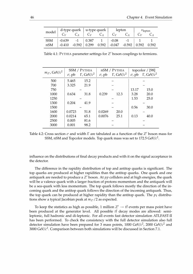
46 Chapter 4. Event Simulation
modeld-type quark u-type quark lepton νleptonCV CA CV CA CV CA CV CA
SSM -0.639 -1 0.387 1 -0.08 -1 1 1nSM -0.410 -0.592 0.299 0.592 -0.047 -0.592 0.592 0.592
Table 4.1: PYTHIA parameter settings for Z′ boson couplings to fermions.
mZ′ , GeV/c2 SSM / PYTHIA nSM / PYTHIA topcolor / [98]σ, pb Γ, GeV/c2 σ, pb Γ, GeV/c2 σ, pb Γ, GeV/c2
500 5.465 15.2 – –700 3.325 21.9 – –750 – – 13.17 15.01000 0.634 31.8 0.239 12.3 3.28 20.01250 – – 1.53 25.01300 0.204 41.9 – –1500 – – 0.56 30.01600 0.0723 51.8 0.0269 20.0 –2000 0.0214 65.1 0.0076 25.1 0.13 40.02500 0.005 81.6 – –3000 0.001 98.2 – –
Table 4.2: Cross section σ and width Γ are tabulated as a function of the Z′ boson mass forSSM, nSM and Topcolor models. Top quark mass was set to 172.5 GeV/c2.
influence on the distributions of final decay products and with it on the signal acceptance inthe detector.
The difference in the rapidity distribution of top and antitop quarks is significant. Thetop quarks are produced at higher rapidities than the antitop quarks. One quark and oneantiquark are needed to produce a Z′ boson. At pp colliders and at high energies, the quarkwill be a valence quark with a larger fraction of protons momentum and the antiquark willbe a sea-quark with less momentum. The top quark follows mostly the direction of the in-coming quark and the antitop quark follows the direction of the incoming antiquark. Thus,the top quark can be produced at higher rapidity than the antitop quark. The pT distribu-tions show a typical Jacobian peak at mZ′/2 as expected.
To keep the statistics as high as possible, 1 million Z′ → tt events per mass point havebeen produced at the generator level. All possible tt decay modes are allowed: semi-leptonic, full hadronic and di-leptonic. For all events fast detector simulation ATLFAST-IIhas been performed. To check the consistency with the full detector simulation also fulldetector simulation have been prepared for 3 mass points, 1000 GeV/c2, 2000 GeV/c2 and3000 GeV/c2. Comparison between both simulations will be discussed in Section 7.1.

4.3 Signal and Background Event Modeling 47
Figure 4.2: The invariant mass mZ′ , rapidity y and pT distributions of top and antitop quarksfor SSM and nSSM modelsand Z′ boson mass of 1000 GeV/c2.
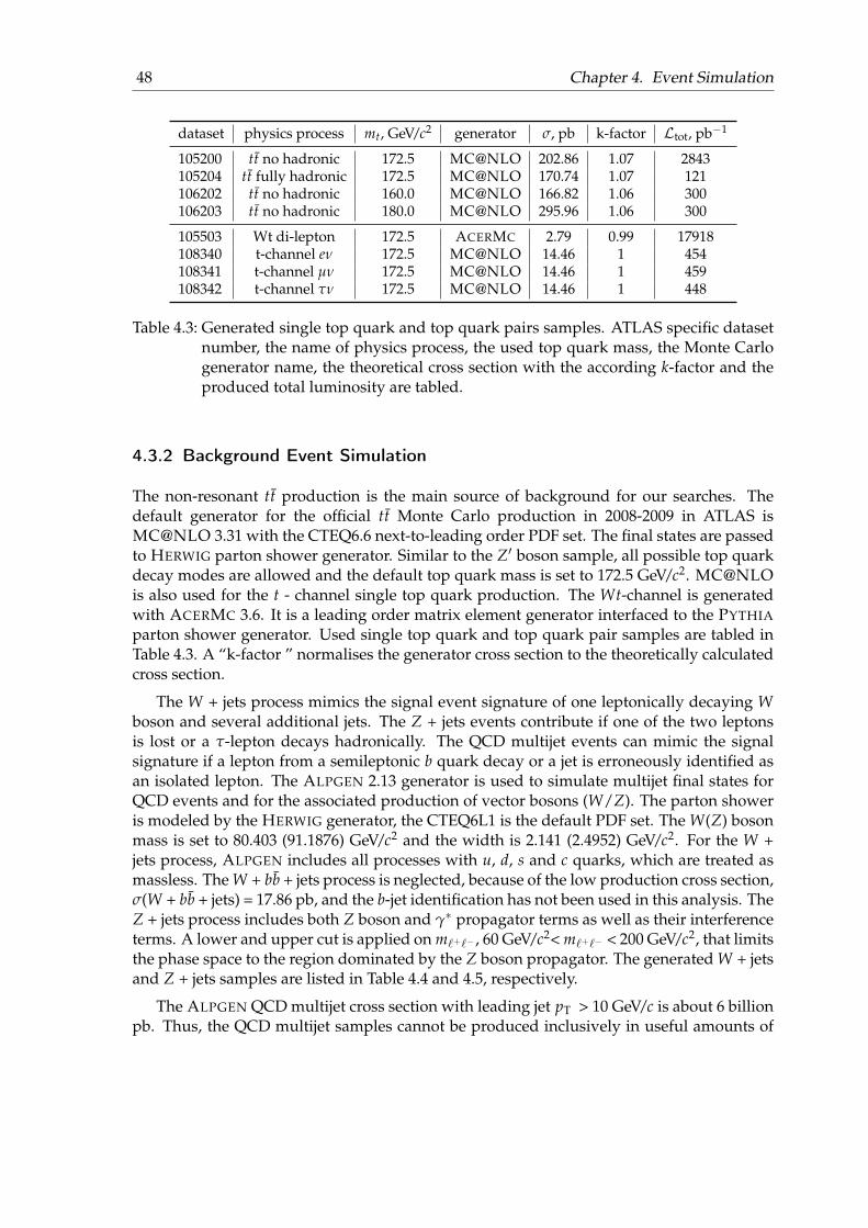
48 Chapter 4. Event Simulation
dataset physics process mt, GeV/c2 generator σ, pb k-factor Ltot, pb−1
105200 tt no hadronic 172.5 MC@NLO 202.86 1.07 2843105204 tt fully hadronic 172.5 MC@NLO 170.74 1.07 121106202 tt no hadronic 160.0 MC@NLO 166.82 1.06 300106203 tt no hadronic 180.0 MC@NLO 295.96 1.06 300
105503 Wt di-lepton 172.5 ACERMC 2.79 0.99 17918108340 t-channel eν 172.5 MC@NLO 14.46 1 454108341 t-channel µν 172.5 MC@NLO 14.46 1 459108342 t-channel τν 172.5 MC@NLO 14.46 1 448
Table 4.3: Generated single top quark and top quark pairs samples. ATLAS specific datasetnumber, the name of physics process, the used top quark mass, the Monte Carlogenerator name, the theoretical cross section with the according k-factor and theproduced total luminosity are tabled.
4.3.2 Background Event Simulation
The non-resonant tt production is the main source of background for our searches. Thedefault generator for the official tt Monte Carlo production in 2008-2009 in ATLAS isMC@NLO 3.31 with the CTEQ6.6 next-to-leading order PDF set. The final states are passedto HERWIG parton shower generator. Similar to the Z′ boson sample, all possible top quarkdecay modes are allowed and the default top quark mass is set to 172.5 GeV/c2. MC@NLOis also used for the t - channel single top quark production. The Wt-channel is generatedwith ACERMC 3.6. It is a leading order matrix element generator interfaced to the PYTHIA
parton shower generator. Used single top quark and top quark pair samples are tabled inTable 4.3. A “k-factor ” normalises the generator cross section to the theoretically calculatedcross section.
The W + jets process mimics the signal event signature of one leptonically decaying Wboson and several additional jets. The Z + jets events contribute if one of the two leptonsis lost or a τ-lepton decays hadronically. The QCD multijet events can mimic the signalsignature if a lepton from a semileptonic b quark decay or a jet is erroneously identified asan isolated lepton. The ALPGEN 2.13 generator is used to simulate multijet final states forQCD events and for the associated production of vector bosons (W/Z). The parton showeris modeled by the HERWIG generator, the CTEQ6L1 is the default PDF set. The W(Z) bosonmass is set to 80.403 (91.1876) GeV/c2 and the width is 2.141 (2.4952) GeV/c2. For the W +jets process, ALPGEN includes all processes with u, d, s and c quarks, which are treated asmassless. The W + bb + jets process is neglected, because of the low production cross section,σ(W + bb + jets) = 17.86 pb, and the b-jet identification has not been used in this analysis. TheZ + jets process includes both Z boson and γ∗ propagator terms as well as their interferenceterms. A lower and upper cut is applied on m`+`− , 60 GeV/c2< m`+`− < 200 GeV/c2, that limitsthe phase space to the region dominated by the Z boson propagator. The generated W + jetsand Z + jets samples are listed in Table 4.4 and 4.5, respectively.
The ALPGEN QCD multijet cross section with leading jet pT > 10 GeV/c is about 6 billionpb. Thus, the QCD multijet samples cannot be produced inclusively in useful amounts of
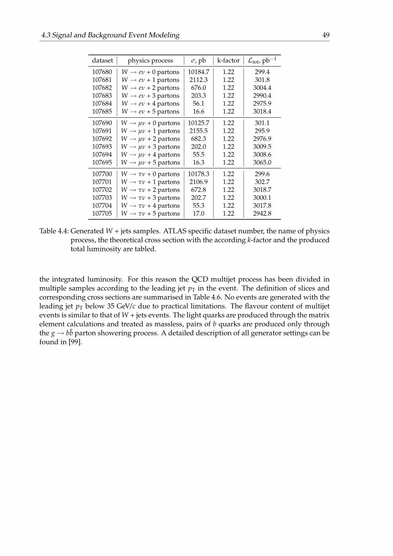
4.3 Signal and Background Event Modeling 49
dataset physics process σ, pb k-factor Ltot, pb−1
107680 W → eν + 0 partons 10184.7 1.22 299.4107681 W → eν + 1 partons 2112.3 1.22 301.8107682 W → eν + 2 partons 676.0 1.22 3004.4107683 W → eν + 3 partons 203.3 1.22 2990.4107684 W → eν + 4 partons 56.1 1.22 2975.9107685 W → eν + 5 partons 16.6 1.22 3018.4
107690 W → µν + 0 partons 10125.7 1.22 301.1107691 W → µν + 1 partons 2155.5 1.22 295.9107692 W → µν + 2 partons 682.3 1.22 2976.9107693 W → µν + 3 partons 202.0 1.22 3009.5107694 W → µν + 4 partons 55.5 1.22 3008.6107695 W → µν + 5 partons 16.3 1.22 3065.0
107700 W → τν + 0 partons 10178.3 1.22 299.6107701 W → τν + 1 partons 2106.9 1.22 302.7107702 W → τν + 2 partons 672.8 1.22 3018.7107703 W → τν + 3 partons 202.7 1.22 3000.1107704 W → τν + 4 partons 55.3 1.22 3017.8107705 W → τν + 5 partons 17.0 1.22 2942.8
Table 4.4: Generated W + jets samples. ATLAS specific dataset number, the name of physicsprocess, the theoretical cross section with the according k-factor and the producedtotal luminosity are tabled.
the integrated luminosity. For this reason the QCD multijet process has been divided inmultiple samples according to the leading jet pT in the event. The definition of slices andcorresponding cross sections are summarised in Table 4.6. No events are generated with theleading jet pT below 35 GeV/c due to practical limitations. The flavour content of multijetevents is similar to that of W + jets events. The light quarks are produced through the matrixelement calculations and treated as massless, pairs of b quarks are produced only throughthe g→ bb parton showering process. A detailed description of all generator settings can befound in [99].
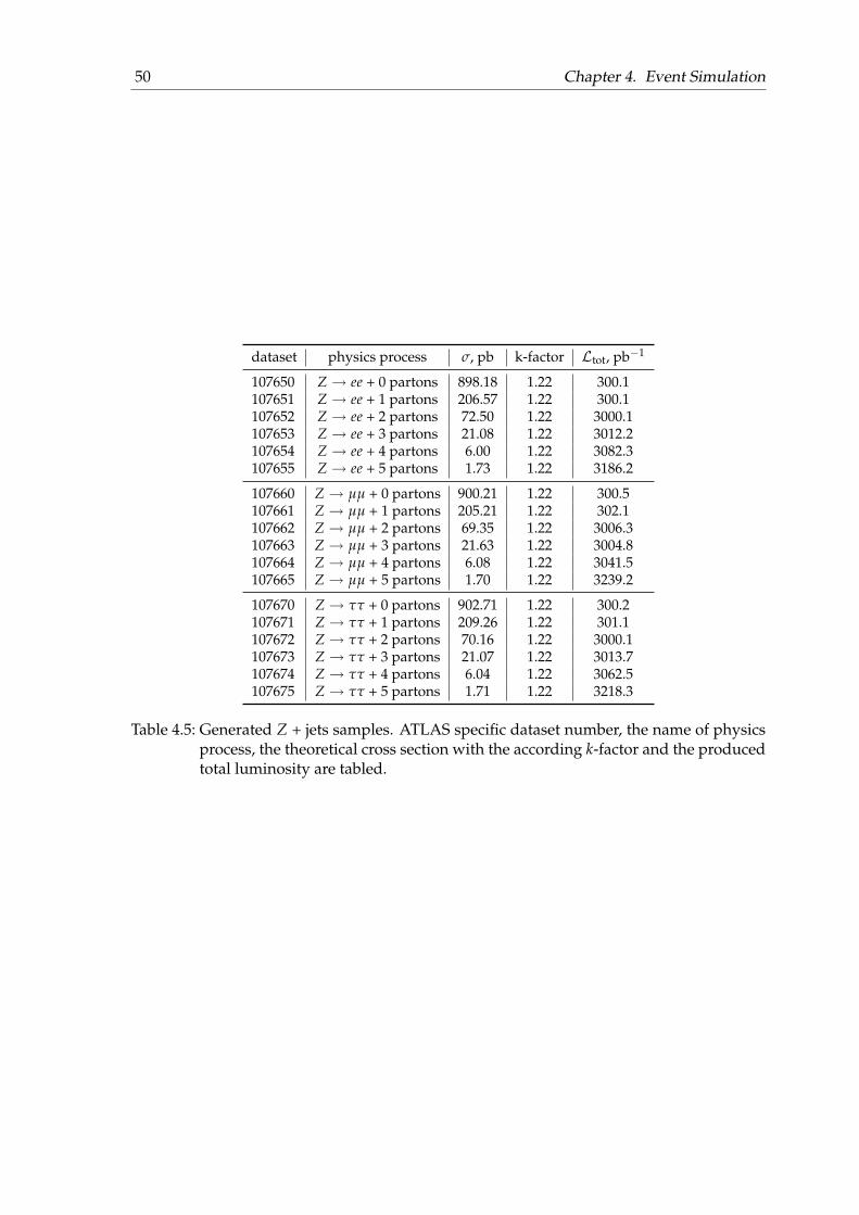
50 Chapter 4. Event Simulation
dataset physics process σ, pb k-factor Ltot, pb−1
107650 Z → ee + 0 partons 898.18 1.22 300.1107651 Z → ee + 1 partons 206.57 1.22 300.1107652 Z → ee + 2 partons 72.50 1.22 3000.1107653 Z → ee + 3 partons 21.08 1.22 3012.2107654 Z → ee + 4 partons 6.00 1.22 3082.3107655 Z → ee + 5 partons 1.73 1.22 3186.2
107660 Z → µµ + 0 partons 900.21 1.22 300.5107661 Z → µµ + 1 partons 205.21 1.22 302.1107662 Z → µµ + 2 partons 69.35 1.22 3006.3107663 Z → µµ + 3 partons 21.63 1.22 3004.8107664 Z → µµ + 4 partons 6.08 1.22 3041.5107665 Z → µµ + 5 partons 1.70 1.22 3239.2
107670 Z → ττ + 0 partons 902.71 1.22 300.2107671 Z → ττ + 1 partons 209.26 1.22 301.1107672 Z → ττ + 2 partons 70.16 1.22 3000.1107673 Z → ττ + 3 partons 21.07 1.22 3013.7107674 Z → ττ + 4 partons 6.04 1.22 3062.5107675 Z → ττ + 5 partons 1.71 1.22 3218.3
Table 4.5: Generated Z + jets samples. ATLAS specific dataset number, the name of physicsprocess, the theoretical cross section with the according k-factor and the producedtotal luminosity are tabled.
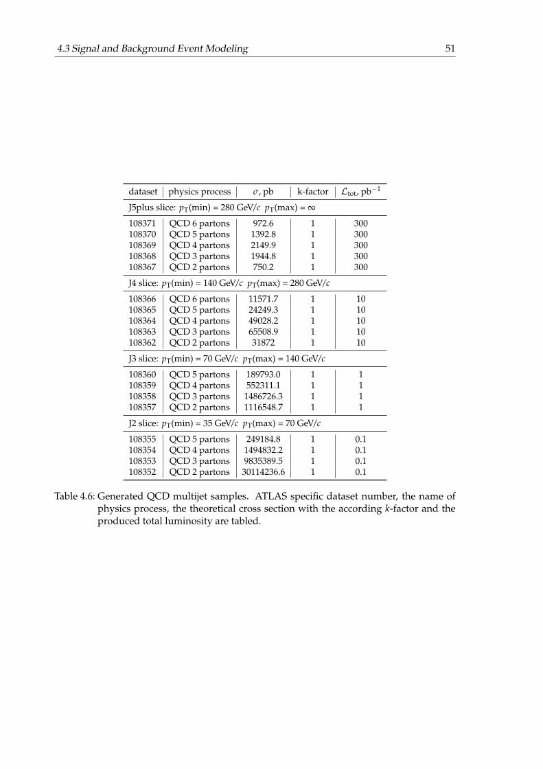
4.3 Signal and Background Event Modeling 51
dataset physics process σ, pb k-factor Ltot, pb−1
J5plus slice: pT(min) = 280 GeV/c pT(max) = ∞
108371 QCD 6 partons 972.6 1 300108370 QCD 5 partons 1392.8 1 300108369 QCD 4 partons 2149.9 1 300108368 QCD 3 partons 1944.8 1 300108367 QCD 2 partons 750.2 1 300
J4 slice: pT(min) = 140 GeV/c pT(max) = 280 GeV/c
108366 QCD 6 partons 11571.7 1 10108365 QCD 5 partons 24249.3 1 10108364 QCD 4 partons 49028.2 1 10108363 QCD 3 partons 65508.9 1 10108362 QCD 2 partons 31872 1 10
J3 slice: pT(min) = 70 GeV/c pT(max) = 140 GeV/c
108360 QCD 5 partons 189793.0 1 1108359 QCD 4 partons 552311.1 1 1108358 QCD 3 partons 1486726.3 1 1108357 QCD 2 partons 1116548.7 1 1
J2 slice: pT(min) = 35 GeV/c pT(max) = 70 GeV/c
108355 QCD 5 partons 249184.8 1 0.1108354 QCD 4 partons 1494832.2 1 0.1108353 QCD 3 partons 9835389.5 1 0.1108352 QCD 2 partons 30114236.6 1 0.1
Table 4.6: Generated QCD multijet samples. ATLAS specific dataset number, the name ofphysics process, the theoretical cross section with the according k-factor and theproduced total luminosity are tabled.

52 Chapter 4. Event Simulation

5 Event Reconstruction
Particles produced in proton-proton collisions go through the detector material and leavesignals in form of electrical charges, which are collected, digitalised and read out by thedetector electronics. Event reconstruction starts with electronic signals in the detector andbuilds physics objects out of it. The aim is to identify the type of objects and to measure theirmomentum and energy with the best possible precision. This chapter describes the signa-ture of different object types in the detector, the algorithms to identify and to reconstructindividual signatures and the corresponding performance. The reconstruction of electons,muons, jets, neutrinos and particle tracks will be discussed, because these objects have beenused for this analysis.
5.1 Track Reconstruction in the Inner Detector
At the design luminosity of 1034 cm−2s−1 about 1000 charged particles will go through theATLAS detector every 25 ns. Such a dense track environment requires high-precision mea-surements as well as a powerful track reconstruction to meet the momentum and vertex res-olution requirements of physics processes. As already discussed in Chapter 3.2, the ATLASinner detector consists of three sub-detectors: the pixel detector, the semiconductor trackerand the transition radiation tracker. The pixel detector delivers directly three-dimensionalmeasurements, measurements in the SCT are transformed into three-dimensional spacepoints combining the information from the opposite sites of a module. The transition ra-diation tracker provides only two-dimensional measurements, but allows an additional dis-crimination between electrons and pions utilising transition radiation in foils and fibres.
Reconstruction of tracks starts with a pattern recognition procedure, which associates de-tector measurements to track candidates. Global methods like histogramming and HOUGH-transform [100] are used to identify all tracks simultaneously. The measurement positionsare transformed from measurement space (measurement coordinates) into track parameterspace (parameters to describe trajectory of a particle). Each measurement corresponds to onecurve. The point where all curves belonging to one track cross corresponds to the param-eter of that track. To find these points, the transformed measurements are histogramised.For example for straight-line tracks the angle between the track and one of the axes is his-togramised. Measurements which belong to one track will peak in the histogram. The pat-tern recognition procedure starts with measurements in the three pixel layer and the firstSCT layer to search for tracks originating from the interaction region. Found seeds are thenextended through the SCT to form track candidates.
After the pattern recognition procedure, many tracks not belonging to any particle, theso-called “ghost” tracks, will be produced. Such tracks will be identified in the track fitting
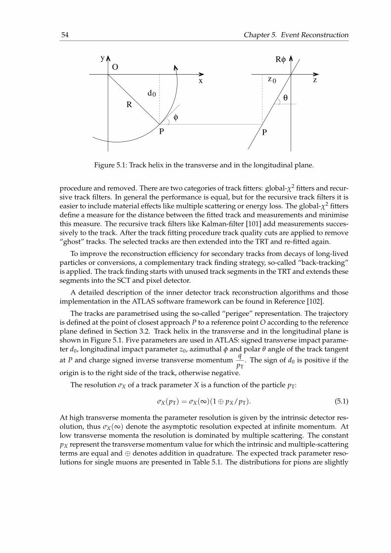
54 Chapter 5. Event Reconstruction
d0
φ
θ
O
P P
z 0
Rφ
z
y
x
R
Figure 5.1: Track helix in the transverse and in the longitudinal plane.
procedure and removed. There are two categories of track fitters: global-χ2 fitters and recur-sive track filters. In general the performance is equal, but for the recursive track filters it iseasier to include material effects like multiple scattering or energy loss. The global-χ2 fittersdefine a measure for the distance between the fitted track and measurements and minimisethis measure. The recursive track filters like Kalman-filter [101] add measurements succes-sively to the track. After the track fitting procedure track quality cuts are applied to remove“ghost” tracks. The selected tracks are then extended into the TRT and re-fitted again.
To improve the reconstruction efficiency for secondary tracks from decays of long-livedparticles or conversions, a complementary track finding strategy, so-called “back-tracking”is applied. The track finding starts with unused track segments in the TRT and extends thesesegments into the SCT and pixel detector.
A detailed description of the inner detector track reconstruction algorithms and thoseimplementation in the ATLAS software framework can be found in Reference [102].
The tracks are parametrised using the so-called “perigee” representation. The trajectoryis defined at the point of closest approach P to a reference point O according to the referenceplane defined in Section 3.2. Track helix in the transverse and in the longitudinal plane isshown in Figure 5.1. Five parameters are used in ATLAS: signed transverse impact parame-ter d0, longitudinal impact parameter z0, azimuthal φ and polar θ angle of the track tangent
at P and charge signed inverse transverse momentumqpT
. The sign of d0 is positive if the
origin is to the right side of the track, otherwise negative.
The resolution σX of a track parameter X is a function of the particle pT:
σX(pT) = σX(∞)(1⊕ pX/pT). (5.1)
At high transverse momenta the parameter resolution is given by the intrinsic detector res-olution, thus σX(∞) denote the asymptotic resolution expected at infinite momentum. Atlow transverse momenta the resolution is dominated by multiple scattering. The constantpX represent the transverse momentum value for which the intrinsic and multiple-scatteringterms are equal and ⊕ denotes addition in quadrature. The expected track parameter reso-lutions for single muons are presented in Table 5.1. The distributions for pions are slightly
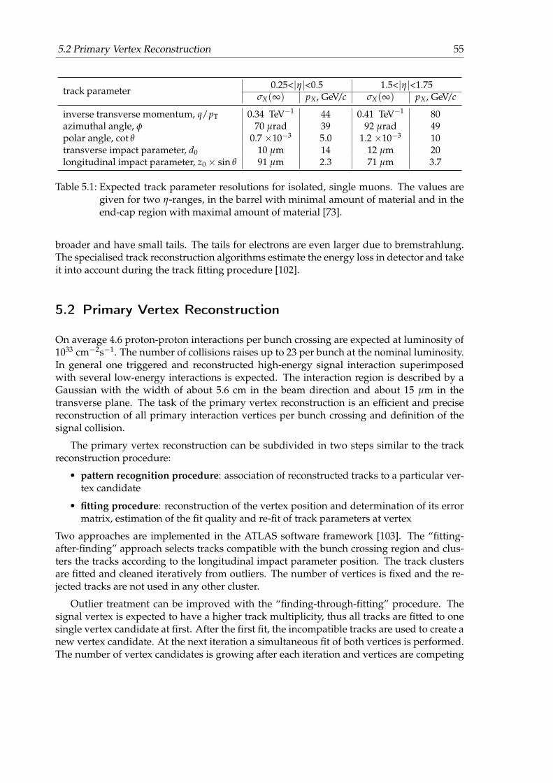
5.2 Primary Vertex Reconstruction 55
0.25<|η|<0.5 1.5<|η|<1.75track parameter
σX(∞) pX, GeV/c σX(∞) pX, GeV/c
inverse transverse momentum, q/pT 0.34 TeV−1 44 0.41 TeV−1 80azimuthal angle, φ 70 µrad 39 92 µrad 49polar angle, cot θ 0.7 ×10⁻³ 5.0 1.2 ×10⁻³ 10transverse impact parameter, d0 10 µm 14 12 µm 20longitudinal impact parameter, z0 × sin θ 91 µm 2.3 71 µm 3.7
Table 5.1: Expected track parameter resolutions for isolated, single muons. The values aregiven for two η-ranges, in the barrel with minimal amount of material and in theend-cap region with maximal amount of material [73].
broader and have small tails. The tails for electrons are even larger due to bremstrahlung.The specialised track reconstruction algorithms estimate the energy loss in detector and takeit into account during the track fitting procedure [102].
5.2 Primary Vertex Reconstruction
On average 4.6 proton-proton interactions per bunch crossing are expected at luminosity of1033 cm−2s−1. The number of collisions raises up to 23 per bunch at the nominal luminosity.In general one triggered and reconstructed high-energy signal interaction superimposedwith several low-energy interactions is expected. The interaction region is described by aGaussian with the width of about 5.6 cm in the beam direction and about 15 µm in thetransverse plane. The task of the primary vertex reconstruction is an efficient and precisereconstruction of all primary interaction vertices per bunch crossing and definition of thesignal collision.
The primary vertex reconstruction can be subdivided in two steps similar to the trackreconstruction procedure:
• pattern recognition procedure: association of reconstructed tracks to a particular ver-tex candidate
• fitting procedure: reconstruction of the vertex position and determination of its errormatrix, estimation of the fit quality and re-fit of track parameters at vertex
Two approaches are implemented in the ATLAS software framework [103]. The “fitting-after-finding” approach selects tracks compatible with the bunch crossing region and clus-ters the tracks according to the longitudinal impact parameter position. The track clustersare fitted and cleaned iteratively from outliers. The number of vertices is fixed and the re-jected tracks are not used in any other cluster.
Outlier treatment can be improved with the “finding-through-fitting” procedure. Thesignal vertex is expected to have a higher track multiplicity, thus all tracks are fitted to onesingle vertex candidate at first. After the first fit, the incompatible tracks are used to create anew vertex candidate. At the next iteration a simultaneous fit of both vertices is performed.The number of vertex candidates is growing after each iteration and vertices are competing

56 Chapter 5. Event Reconstruction
with each other to obtain more tracks. The vertex with the largest sum of squared transversemomenta of all associated tracks ∑ p2
T is defined as the signal vertex.
The performance of the primary vertex reconstruction is physics process dependent. Thereconstruction efficiency for tt events is 100% and the selection efficiency of the signal vertexis around 99%. The position resolution in the transverse plane to the beam axis is 11 µm andalong the beam axis 40 µm [73].
5.3 Charged Lepton Identification
As the expected Z′ boson production cross section is small, an excellent lepton identificationespecially at high transverse momenta is crucial. In the next two sections the electron andmuon reconstruction and identification relevant for this analysis will be described.
Reconstruction and Identification of Electrons
Electrons are charged particles which leave tracks in the inner detector and induce showerin the electromagnetic calorimeter. Electrons going through matter primarily emit photonsin the bremstrahlung process. Photons convert into an electron-positron pair, the producedelectrons and positrons emit photons again. The pair production and the bremstrahlungcontinue in turn, until produced particles are absorbed by atoms. Therefore, the electro-magnetic showers induced by electrons and photons are very similar. Photons are neutralparticles and do not produce tracks as long as they do not convert in the material of the innerdetector. To distinguish between electrons and photons we require a track not associated toa photon conversion.
Reconstruction of electrons starts from clusters reconstructed in the electromagneticcalorimeter. Electron identification variables are build from track properties and measure-ments in the calorimeters. An electromagnetic tower seed with transverse energy above∼ 3 GeV and a matching track which do not belong to a photon conversion in the materialof the inner detector are required for an electron candidate. A track extrapolated to the elec-tromagnetic calorimeter must match the cluster in the middle layer in a ∆η × ∆φ windowof 0.05 × 0.10. The ratio of energy of the cluster to the momentum of the track is requiredto be lower than 10. The selection efficiency of true isolated electrons with ET> 20 GeV and|η| < 2.5 is about 93%. The inefficiency is caused mainly by the large amount of material inthe inner detector.
The signal in the electromagnetic calorimeter induced by electrons has to be distin-guished from the shower induced by hadrons like pions or protons. Due to the design ofthe ATLAS detector, hadrons go first through the electromagnetic calorimeter and deposita small amount of their energy in the electromagnetic calorimeter. In general the width ofan electron shower is narrower than for hadrons. Electrons leave a core with a high activitysurrounded by a small area with low activity in the calorimeter. Additionally hadron show-ers are often produced by several particles which belong to one jet and thus their shower isbroader. It is more difficult to discriminate between single pions decaying into two photonsand isolated electons. The granularity of the electromagnetic calorimeter is high enough to

5.3 Charged Lepton Identification 57
resolve both photons. Counting the number of energy maxima found in the electromag-netic shower allows to identify single electrons. As the main part of the energy deposit ofhadrons is in the hadronic calorimeter, a good discriminant is the ratio of the energy storedin the hadronic calorimeter to the energy stored in the electromagnetic calorimeter, the so-called hadronic leakage. Also the ratio of energy deposit in electromagnetic calorimeter tothe track momentum for charged hadrons is much lower than for electrons.
To identify true high-pT electrons, three sets of selection criteria, loose, medium andtight, have been defined, depending on the electron identification efficiency and the cor-responding background rejection rate. This provides some flexibility in the choice of anoptimal electron selection depending on the process we are interested in. The standard elec-tron identification is based on cuts, optimised in up to seven bins in η and up to six bins inpT. Briefly summarised, the selection criteria are:
• loose electron selection criteria
– detector acceptance within |η| < 2.47– hadronic leakage– ratio in η of cell energies in 3×7 versus 7×7 cells from the middle layer of elec-
tromagnetic calorimeter– ratio in φ of cell energies in 3×3 versus 3×7 cells from the middle layer of elec-
tromagnetic calorimeter– lateral width of shower
• medium electron selection criteria
– includes loose cuts– difference between the second largest energy deposit in a window ∆η × ∆φ =
0.125× 0.2 around the cell with the highest ET and the minimal energy betweenthe first and the second maxima
– second largest energy deposit normalised to the cluster energy– total shower width– shower width over three strips in the first layer of elecromagnetic calorimeter
around the one with the maximal energy deposit– fraction of energy deposited outside the shower core of three central strips but
within seven strips– track quality cuts: at least one pixel hit, at least nine pixel and SCT hits and trans-
verse impact parameter < 1 mm
• tight electron selection criteria
– includes medium cuts– at least one hit in the first pixel layer– total number of hits in the TRT– ratio of high-threshold hits in the TRT to the total number of hits in the TRT– ∆η < 0.005 and ∆φ < 0.02 between the cluster and the matched track– ratio of the cluster energy to the track momentum– two different cuts optimised for the isolated and non-isolated electrons in jets: in
case of isolated electrons additional cut on the ratio of transverse energy in a cone

58 Chapter 5. Event Reconstruction
Figure 5.2: Electron identification efficiency as a function of ET (left) and η (right) for elec-trons from Z′ → e+e− events [73].
∆R < 0.2 to the total cluster transverse energy is applied. In case of non-isolatedelectrons tighter TRT cuts are required
The medium and loose electron reconstruction efficiency for Z′→ e+e− process in ET andη bins is presented in Figure 5.2. The loose electron selection provides the best efficiency, buta low jet rejection rate. For example the loose reconstruction efficiency in Z→ e+e− processis about 88% and the jet rejection rate 1/εjet is ∼ 570 [73]. The medium selection improvesthe background rejection by a factor of 3-4 and leads to a moderate efficiency loss of ∼ 10%.For a tight selection the electron identification efficiency drops down to 61 - 65%, but the jetrejection rate is of order 105. For this analysis electrons with medium quality cuts will beused. This provides a good selection efficiency and a reasonable jet rejection rate.
Reconstruction and Identification of Muons
The primary system to detect muons is the muon spectrometer. It has been designed toidentify muons with pT above 3 GeV/c and covers the pseudorapidity range |η| < 2.7. Themuon spectrometer provides a precise measurement of muon momentum up to 1 TeV/c. Atlow momentum, the resolution is mainly limited by the energy loss in the material in frontof spectrometer. In the intermediate range the multiple scattering in the spectrometer playsa decisive role. At very high transverse momenta above 300 GeV/c, prevails the single hitresolution.
Other parts of the ATLAS detector have an impact on the muon reconstruction, too. Thecalorimeter absorbs hadrons, electrons and photons, thus the rate of particles except muonsis reduced significantly before entering the spectrometer. The characteristic minimum ion-ising signature of muons in the calorimeter can be aid in the muon identification. Directmeasurement of the muon energy lost in the calorimeter improves the energy resolution.The inner detector provides an independent and very precise momentum measurement formuons as well a confirmation of the spectrometer measurement, but in a reduced |η| < 2.5range.

5.4 Jet Reconstruction 59
η-3 -2 -1 0 1 2 3
effic
ienc
y
0
0.5
1
foundgood
ATLAS directtt
Staco
(GeV/c)T
p0 50 100 150 200
res
olut
ion
Tp
0
0.01
0.02
0.03
0.04
0.05
0.06ATLAS
directttStaco
Figure 5.3: Combined muon reconstruction efficiency in tt events for “Staco” algorithm andmuon momentum resolution as function of η [73]. For “good”muons a gooddistance match (χ2 < 4.5) between reconstructed and truth track is required.
The muon momentum resolution is improved by a combination of measurements inthe inner detector and in the spectrometer for muons with transverse momenta between30 GeV/c and 200 GeV/c. At transverse momenta below 30 GeV/c the resolution achieved inthe inner detector is better than in the spectrometer. At very high momenta above 200 GeV/c,the spectrometer has better performance due to the longer lever arm.
As shown in Figure 5.3, the muon reconstruction efficiency is close to 100% except inregions where the detector coverage is poor, that is for |η| around 0.0 and 1.2. On averagethe reconstruction efficiency in tt events is 94.3% and for high pT muons from the Z′ bosondecay is 91.0%. The transverse momentum resolution σpT /pT is around 3-4% for muon pTbelow 200 GeV/c and increases up to 10% at 1 TeV/c. Mis-reconstruction and charge misiden-tification rates are around 0.01%.
5.4 Jet Reconstruction
Jet algorithms define the jets. They provide a set of rules that indicate how close two parti-cles must be to belong to one jet and how the momentum of the combination is calculated. Ajet algorithm should fulfill several requirements, which become apparent in different appli-cation of jets in the experiments and in theory. The jet definition should be mostly indepen-dent of the non-perturbative effects like hadronisation and underlying event. The measuredobservables should be comparable to the theoretical calculations. Addition of an infinitesoft parton (infrared safety, illustrated in Figure 5.5(a)) or a parton radiated by an infinitesmall angle (collinear safety, illustrated in Figure 5.5(b)) should not change properties andnumber of resulting jets and they should be independent of the detector details.
At the LHC a new energy regime will be explored, heavy particles like W and Z bosonsor top quarks will be produced relatively often at high transverse momenta. Their hadronicdecay products may form single jets with a complex substructure. To study such substruc-tures, we need a suitable jet finder. In the ATLAS reconstruction framework the same jetfinder can be run on miscellaneous objects like calorimeter signal towers, topological cell

60 Chapter 5. Event Reconstruction
(a) infrared safety
(b) collinear safety
Figure 5.4: (a) Illustration of infrared sensitivity: the arrows represent seed particles, a softradiated parton causes a merging of the seeds in one jet. (b) Illustration of thecollinear sensitivity: the splitting into two particles changes the number of jets orjet properties.
clusters in the calorimeters, reconstructed tracks, generator particles and partons. A well-maintained open-source software package FastJet [104] is used for all jet finder implemen-tations, except for the ATLAS Cone algorithm.
A common feature of all jet finder implementations in ATLAS is the full four-momentumrecombination scheme. This scheme conserves energy and momentum and provides ameaningful single-jet mass. The algorithms can be divided in two broad categories. Thefirst category is based on the energy flow into a geometric cone (cone algorithms) and thesecond one on the recombination of the closest pairs of the particles (cluster algorithms).
ATLAS Cone Algorithm
There is a wide range of “cone algorithms” based on the maximisation of the energy in ageometric cone. The key parameter of the cone algorithms is the radius of the cone in the(η − φ)-plane, Rcone. The ATLAS cone algorithm uses seeds in order to initiate the first conecandidates. The seed is a calorimeter tower or cluster, parton or particle with ET or pT abovethe seed threshold. All objects with a distance R smaller than the fixed cone size Rcone will becombined with the seed. The direction of the seed is updated from the four-momenta of theconstituents inside the initial cone and a new cone is centred around it. The recombinationcontinues until a seed with a stable direction is found. This procedure is repeated for all

5.4 Jet Reconstruction 61
founded seeds. The seeds can share the constituents, the ambiguities are solved in the lastso-called “split and merge” step. The jets which share constituents with 50% of ET or pT ofthe lowest energy jet will be merged.
The seeded cone algorithms are not infrared safe. An additional soft particle, actingas a new seed, can cause the iterative process to find a new stable cone. This can lead inthe split-merge step to the modification of the final jets. The ATLAS cone algorithm is stillused in many physics analysis for more or less historical reasons. The ATLAS performancegroup responsible for the jet and missing transverse energy calibration has established nowthe Anti-kT jet algorithm, which belongs to the second category of the jet reconstructionalgorithms.
Cluster Algorithms
The cluster algorithms are based on the pair-wise clustering of initial constituents. The keyparameters are a distance measure between the objects and some condition upon whichclustering should not be carried out. The distance measures dij between two objects i and jand diB between the object i and the beam, are defined as:
dij = min(
p2mTi , p2m
Tj
) (∆R)2ij
R2 , (5.2)
diB = p2mTi , (5.3)
where (∆R)2ij is the distance between two objects in the (η − φ)-plane. The d values are com-
puted for all possible combinations. If dij is the smallest value, objects i and j are combinedusing four-momentum combination and the remaining combinations are recalculated. If thesmallest value is diB, this object is considered as a jet and is removed from the initial objects.The variable R defines the resolution at which jets are resolved from each other comparedto the beam.
There are three different cluster algorithms, depending on the value of variable m:
• kT algorithm [105, 106] with m = 1,
• Anti-kT algorithm [107] with m = −1,
• Cambridge/Aachen algorithm [108, 109] with m = 0.
If m = 1, the objects with low relative pT are merged first and the final merge is thehardest one. In some sense this procedure is inverse to the splitting within a parton showerand provides a tool to analyse the substructure of jets. Not merged soft partons will berejected by a final pT cut and associated with the beam.
If m = −1, the soft objects will tend to cluster with the hard ones, long before theycluster among themselves. The hard objects will accumulate all soft ones within a cone ofradius R, if no hard neighbours are within 2R. The result will be a perfectly conical jet.Two comparably hard objects within R < ∆R < 2R will share the energy between themdepending on the relative pT and the distance. The hard objects within ∆R < R will bemerged in one single jet.

62 Chapter 5. Event Reconstruction
For m = 0 the pT of the objects is irrelevant and the clustering will be carry out accordingto the angular distance R between two objects, starting with the closest one. This algorithmcan improve the single-jet mass resolution, removing small and peripheral subjets.
All three cluster algorithms are infrared and collinear safe. The Anti-kT algorithm ismost preferred one at ATLAS. Studies in Reference [110] demonstrate that the Anti-kT jetsare less affected by underlying event and pileup effects and show best performance for alljet flavours, fragmentation and showering models in terms of reconstruction efficiency. Thejet area is the most stable and should be the easiest to calibrate.
Calorimeter Jets
The jets are reconstructed with the jet algorithms described above using calorimeter signals.The ATLAS calorimeter is a complex system with about 200 000 cells. The cells are combinedinto a larger signal objects, which are the input for the jet finder. There are two concepts forthe combination: signal towers and topological cell cluster.
• signal towers: The calorimeter cells are projected onto a grid in the (η, φ)-plane asillustrated in Figure 5.6(a). The towers have a fixed size of ∆η × ∆φ = 0.1× 0.1. Thewhole acceptance region is divided uniform in 6 400 towers in total. The signal cellscontribute their total raw signal as measured in the calorimeter to the tower signal,weighted by the overlap fraction of the cell area with the towers. The energy scale ofthe raw signal is called electromagnetic (EM) energy scale. No further corrections orcalibrations are applied at this stage.
• topological cell cluster: The signal cells are clustered to three-dimensional “energyblobs”, representing the particle showering in the calorimeter. The clustering startswith the seed cells, whose signal significance defined as the cell energy Ecell dividedby the cell noise σnoise, Γ = Ecell/σnoise, is above a certain threshold, |Γ| > 4. All directneighbours are collected first. Neighbours of neighbours are added to the cluster iftheir signal is above a secondary threshold, |Γ| > 2. Finally, the ring of guard cellswith the significance |Γ| > 0 are added. Afterwards the initial clusters are analysedfor the local signal maxima and splitted if any are found. An example of reconstructedclusters is illustrated in Figure 5.6(b).
In the pseudorapidity range 1.5 . |η| . 2.5 single particles can be resolved by theclustering algorithm. In the central region |η| . 1.5 the cell size is a bit larger and theshower of single particles may overlap. On average 1.6 particles are reconstructed in onecluster. In the forward region |η| & 2.5 the linear distance between the particles is smallerand the calorimeter cells are larger. Either leads to a worse resolution.
Similar to the tower signals, the topological cell clusters are build from the cell signalsat the EM scale. Additionally the energy can be calibrated to a local hadronic energy scale.The clusters are classified as electromagnetic, hadronic and noise. The energy of hadronicclusters is corrected according to their location and the signal shape. The energy lost in thedead material is corrected for all clusters. The correction functions are based on the singleparticle simulations.

5.4 Jet Reconstruction 63
(a) signal towers (b) signal clusters
Figure 5.5: (a) Building of signal towers, cells contribute with their total signal weighted bythe overlap fraction wcell. (b) Building of signal clusters, cells contribute onlywhen their signal significance is above a certain threshold. Thus clusters havenoise suppression build in.
Jet Reconstruction Flow
The jet reconstruction flow is sketched in Figure 5.6. It starts from calorimeter towersor topological clusters measured at the EM scale. The charge output for hadrons in thecalorimeter is smaller than for electrons and has to be corrected to the hadronic energy scale.The way how to calibrate hadronic signals will be discussed a bit later. The tower signalsare only on the EM scale. The topological clusters are either on this scale or are calibratedon a local hadronic energy scale. Signal fluctuations from noise can lead to a negative towersignal. Combination of negative signal towers with nearby positive signal towers cancelsmost of the fluctuations. Only negative signal towers without nearby positive towers aredropped. The topological clusters have noise suppression build in.
Towers or clusters are input to the jet finding algorithms. The output are calorimeterjets on the electromagnetic energy scale or already fully calibrated calorimeter jets on thehadronic energy scale. On the non-calibrated calorimeter jets cell weighting technique is ap-plied [111]. The signal in each calorimeter cell i is weighted depending on the cell locationand the cell signal density ρi = Ei/Vi, where Ei is the energy in the cell on the electro-magnetic scale and Vi is its volume. For the high signal densities more likely generated byelectrons the weighting factor is around 1. It raises up to 1.5, the typical electron/pion signalratio for the ATLAS calorimeter for decreasing cell signal densities more likely generated byhadrons. The weighting functions are determined using the cone Rcone= 0.7 jets in fully sim-ulated QCD di-jet events by fitting the reconstructed calorimeter tower jet energies to thematched Monte Carlo truth particle jet energies.
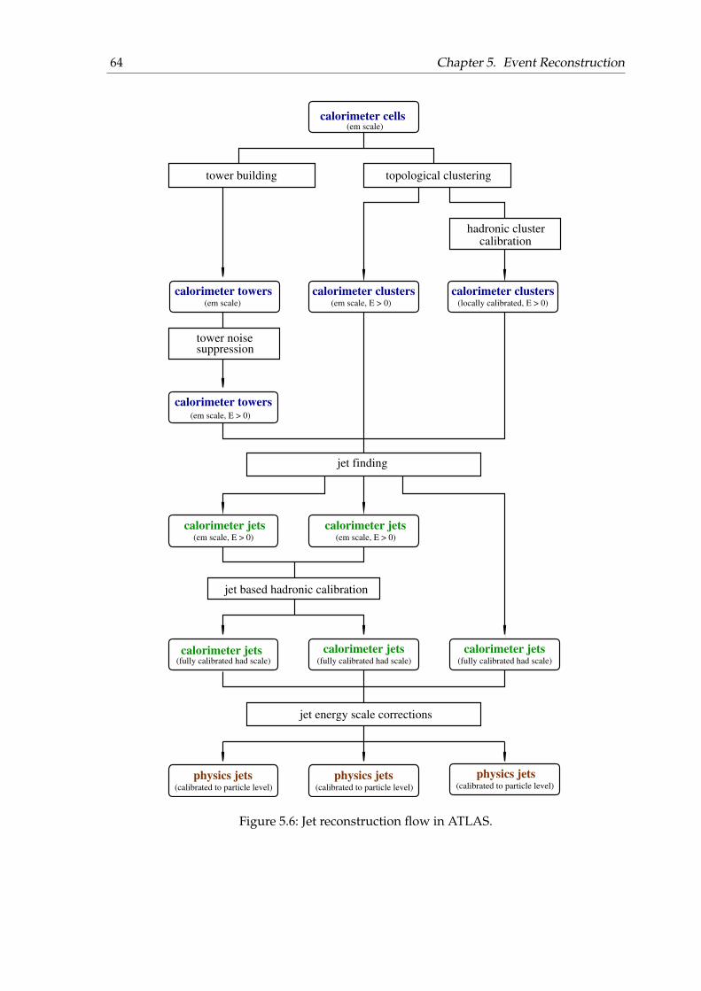
64 Chapter 5. Event Reconstruction
(em scale)calorimeter cells
tower building topological clustering
hadronic clustercalibration
(locally calibrated, E > 0)
calorimeter clusterscalorimeter clusters(em scale, E > 0)
calorimeter towers(em scale)
suppressiontower noise
calorimeter towers(em scale, E > 0)
jet finding
jet based hadronic calibration
calorimeter jets calorimeter jets(em scale, E > 0)(em scale, E > 0)
jet energy scale corrections
(calibrated to particle level) (calibrated to particle level) (calibrated to particle level)physics jets physics jets physics jets
calorimeter jets(fully calibrated had scale)
calorimeter jets(fully calibrated had scale)
calorimeter jets(fully calibrated had scale)
Figure 5.6: Jet reconstruction flow in ATLAS.
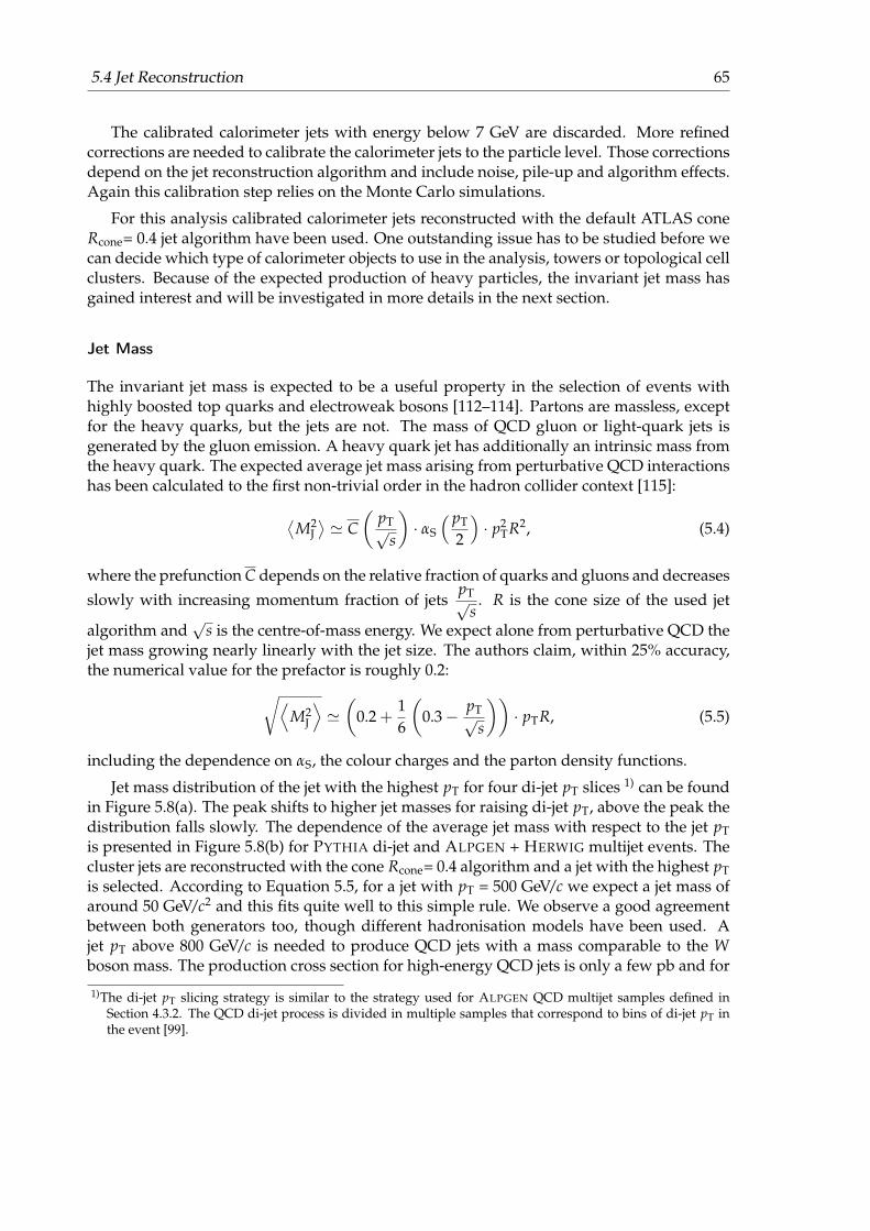
5.4 Jet Reconstruction 65
The calibrated calorimeter jets with energy below 7 GeV are discarded. More refinedcorrections are needed to calibrate the calorimeter jets to the particle level. Those correctionsdepend on the jet reconstruction algorithm and include noise, pile-up and algorithm effects.Again this calibration step relies on the Monte Carlo simulations.
For this analysis calibrated calorimeter jets reconstructed with the default ATLAS coneRcone= 0.4 jet algorithm have been used. One outstanding issue has to be studied before wecan decide which type of calorimeter objects to use in the analysis, towers or topological cellclusters. Because of the expected production of heavy particles, the invariant jet mass hasgained interest and will be investigated in more details in the next section.
Jet Mass
The invariant jet mass is expected to be a useful property in the selection of events withhighly boosted top quarks and electroweak bosons [112–114]. Partons are massless, exceptfor the heavy quarks, but the jets are not. The mass of QCD gluon or light-quark jets isgenerated by the gluon emission. A heavy quark jet has additionally an intrinsic mass fromthe heavy quark. The expected average jet mass arising from perturbative QCD interactionshas been calculated to the first non-trivial order in the hadron collider context [115]:
⟨M2
J⟩' C
(pT√
s
)· αS
( pT
2
)· p2
TR2, (5.4)
where the prefunction C depends on the relative fraction of quarks and gluons and decreases
slowly with increasing momentum fraction of jetspT√
s. R is the cone size of the used jet
algorithm and√
s is the centre-of-mass energy. We expect alone from perturbative QCD thejet mass growing nearly linearly with the jet size. The authors claim, within 25% accuracy,the numerical value for the prefactor is roughly 0.2:√⟨
M2J
⟩'(
0.2 +16
(0.3− pT√
s
))· pTR, (5.5)
including the dependence on αS, the colour charges and the parton density functions.
Jet mass distribution of the jet with the highest pT for four di-jet pT slices 1) can be foundin Figure 5.8(a). The peak shifts to higher jet masses for raising di-jet pT, above the peak thedistribution falls slowly. The dependence of the average jet mass with respect to the jet pTis presented in Figure 5.8(b) for PYTHIA di-jet and ALPGEN + HERWIG multijet events. Thecluster jets are reconstructed with the cone Rcone= 0.4 algorithm and a jet with the highest pTis selected. According to Equation 5.5, for a jet with pT = 500 GeV/c we expect a jet mass ofaround 50 GeV/c2 and this fits quite well to this simple rule. We observe a good agreementbetween both generators too, though different hadronisation models have been used. Ajet pT above 800 GeV/c is needed to produce QCD jets with a mass comparable to the Wboson mass. The production cross section for high-energy QCD jets is only a few pb and for
1)The di-jet pT slicing strategy is similar to the strategy used for ALPGEN QCD multijet samples defined inSection 4.3.2. The QCD di-jet process is divided in multiple samples that correspond to bins of di-jet pT inthe event [99].

66 Chapter 5. Event Reconstruction
(a) jet mass distributions (b) average jet mass
(c) jet mass ratio
Figure 5.7: (a) PYTHIA QCD jet mass distributions of the highest pT jet for several jet pTslices. (b) Average jet mass distribution of highest pT jet in QCD events generatedwith PYTHIA and ALPGEN. (c) Ratio of the reconstructed jet mass for tower andcluster jets to truth jet mass at generator level as a function of jet pT in Z′ → ttevents. Reconstructed jets are matched to truth jets requiring ∆R < 0.2
the first resonance searches in the semi-leptonic channel neglectable, but we should keep inmind that the QCD jets are not massless.
From the experimental point of view, the jet mass reconstruction is a challenging task.To get a perfect jet mass resolution, all hadrons in jet have to be reconstructed as preciselyas possible. Due to the showering and resulting overlap of signals in the calorimeter, thejet mass will be smeared. In the pseudorapidity range 1.5 . |η| . 2.5 single particles canbe resolved, but in the central and in the forward region the calorimeter cells are too large

5.5 Neutrino Reconstruction 67
to resolve single particles. Low-energy particles with pT < 500 MeV/c will be bend by themagnetic field in the inner detector and get lost for the jet reconstruction. Dead materialin the detector will absorb the low-energy photons. The reconstructed jet mass agrees withthe true jet mass within 10% as presented in Figure 5.8(c). At jet transverse momenta below100 GeV/c, the jet mass is underestimated, at higher pT overestimated. The ratio mreco jet
mtruth jetis
closer to 1 for tower jets, because tower truth jets have been used to calibrate the jet energyscale. Thus, for this analysis the tower jets will be used.
5.5 Neutrino Reconstruction
The interaction probability for neutrinos with the material of the detector is close to zero.Therefore they can be reconstructed only indirectly from the total energy balance of theevent. The longitudinal component of the energy in hadron-hadron collisions is unknown,since the colliding partons carry only a fraction of the energy of the hadrons. But the initialtransverse component is zero and the transverse energy balance can be used to reconstructat least the transverse energy of neutrino, so-called ~Emiss
T .
A precise measurement of the missing transverse energy is essential for the QCD mul-tijet background suppression. The main challenge is to minimise the impact of the limiteddetector coverage, finite detector resolution, presence of dead regions and noise in the de-tector that can produce fake ~Emiss
T . The transverse missing energy is primarily reconstructedfrom the energy deposits in the calorimeter and reconstructed muon tracks. The calorimeterextends to a large pseudorapidity range and detects particles even in the very forward re-gion. There are several inactive transition regions between different parts of the calorimeter,which have to be taken into account. Also dead and noisy readout channels contribute tofake ~Emiss
T .
Two algorithms are available to reconstruct missing transverse energy. One uses thecalorimeter cells as input and the other uses the reconstructed objects. The object-based ~Emiss
Treconstruction is used for analyses that are sensitive to low-pT deposits coming from pions,soft jets, the underlying event and from pile-up. A detailed description for the object-basedalgorithm can be found in [73], for this analysis only the cell-based method is used. Thecell-based missing energy reconstruction starts with cells that survive the noise suppressionprocedure and sums up the transverse energy deposits in the calorimeter, corrected by theenergy lost in the cryostat and energy of measured muons.
The calorimeter cells are calibrated depending on the nature of the shower - electromag-netic or hadronic one. Muons reconstructed in the muon spectrometer and with a matchedtrack in the inner detector are considered. But only the energy measurement in the spectrom-eter is taken, hence the energy lost in the calorimeter is already included. The energy of jets iscorrected by the energy lost in the cryostat between electromagnetic and hadronic calorime-
ter. Already at this point a good linearity|~Emiss
T |(true)− |~EmissT |(reco)
|~EmissT |(true)
and a good energy
resolution is achieved. Finally the calorimeter cells are associated with the reconstructedand identified high-pT objects, in a chosen order: electrons, photons, muons, hadronicallydecaying τ-leptons, b-jets and light jets. Refined calibration of the objects is used to improve

68 Chapter 5. Event Reconstruction
(GeV)missT
True E0 50 100 150 200 250 300
Line
arity
of r
espo
nse
-0.3
-0.2
-0.1
0
0.1
0.2
0.3
refined calibrationmissTE
calibration at EM scalemissTE
global calibrationmissTE
(a) linearity
(GeV)T EΣ0 200 400 600 800 1000 1200 1400 16001800 2000
Res
olut
ion
(GeV
)
0
5
10
15
20
25
30
35
40QCD Jets
SUSY
tt
ττ→A
(b) resolution
Figure 5.8: (a) Linearity of reconstructed missing transverse energy for different physics pro-cesses as a function of true missing transverse energy at different calibrationstages. (b) Missing transverse energy resolution as a function of the total trans-
verse energy. The curve corresponds to σ = 0.57√
∑ ET fit [73].
the global calibration of calorimeter cells. For calorimeter cells not associated with any re-constructed high-pT objects only the global calibration can be used. The linearity of responsefor reconstructed ~Emiss
T at different calibration stages as well as the EmissT = |~Emiss
T | resolutionis presented in Figure 5.8. Refined Emiss
T calibration shows the best results compared to thecalibration at the earlier stages. For Emiss
T above 40 GeV, the linearity is within 2%, at lowermissing transverse energies the measurement is biased due to the finite resolution. The Emiss
T
resolution behaves close to σ = 0.57√
∑ ET. Only at very low EmissT values, where the con-
tribution of noise is more important, and at very high EmissT values, where the constant term
in the resolution dominates, we observe a stronger deviation from the√
∑ ET behaviour.
Reconstruction of the longitudinal component of the neutrino momentum pz,ν is onlypossible when some additional information is taken into account. In our case the neutrinois coming from the W boson decay. Thus, assuming the W boson is produced on-shell, wecan use its pole mass mW= 80.4 GeV/c2 as constraint to obtain an equation for the missinglongitudinal component of the neutrino momentum. The sum of the four-vectors of thelepton p` and the neutrino pν is equal to the four-vector of the W boson pW :
pW = p` + pν. (5.6)
After squaring the equation, rearranging its terms and neglecting the invariant masses ofthe lepton and the neutrino, a quadratic equation in pz,ν is obtained:
p2z,ν − 2 · µpz,`
E2` − p2
z,`· pz,ν +
E2` p2
T,ν − µ2
E2` − p2
z,`= 0, (5.7)
with µ =12
m2W + pT,`pT,ν cos ∆φ, (5.8)

5.5 Neutrino Reconstruction 69
where the azimuthal angle difference between the missing transverse energy and the leptonis given by ∆φ. E` is the energy and pz,` is the longitudinal component of the lepton mo-mentum and pT,ν is the transverse component of the neutrino momentum. Equation 5.7 issolved by
p±z,ν =µpz,`
pT,`±
√√√√µ2 p2z,`
p4T,`−
E2` p2
T,ν − µ2
p2T,`
. (5.9)
If the radicand is positive, we retrieve two real solutions. The solution with the smallerabsolute value is taken, because in about 70% of tt events the smaller solution leads to valuesclose to the true values. But if the reconstructed transverse mass of the W boson mT,W
m2T,W = E2
T,W − ~pT,W = 2pT,`pT,ν(1− cos ∆φ) (5.10)
exceeds the pole mass and the radicand becomes negative, the solutions become complex.The width of the W boson is too narrow to explain the large values of mT,W and the mainreason is the imperfect reconstruction of the missing transverse energy. An approach hasbeen developed in [116] to handle complex solutions. The idea is to modify the Emiss
x andEmiss
y components, so that the resulting solution for the longitudinal component becomesreal. It has been shown that the modified values for the transverse missing energy are closerto the true values and improve the missing energy reconstruction.

70 Chapter 5. Event Reconstruction
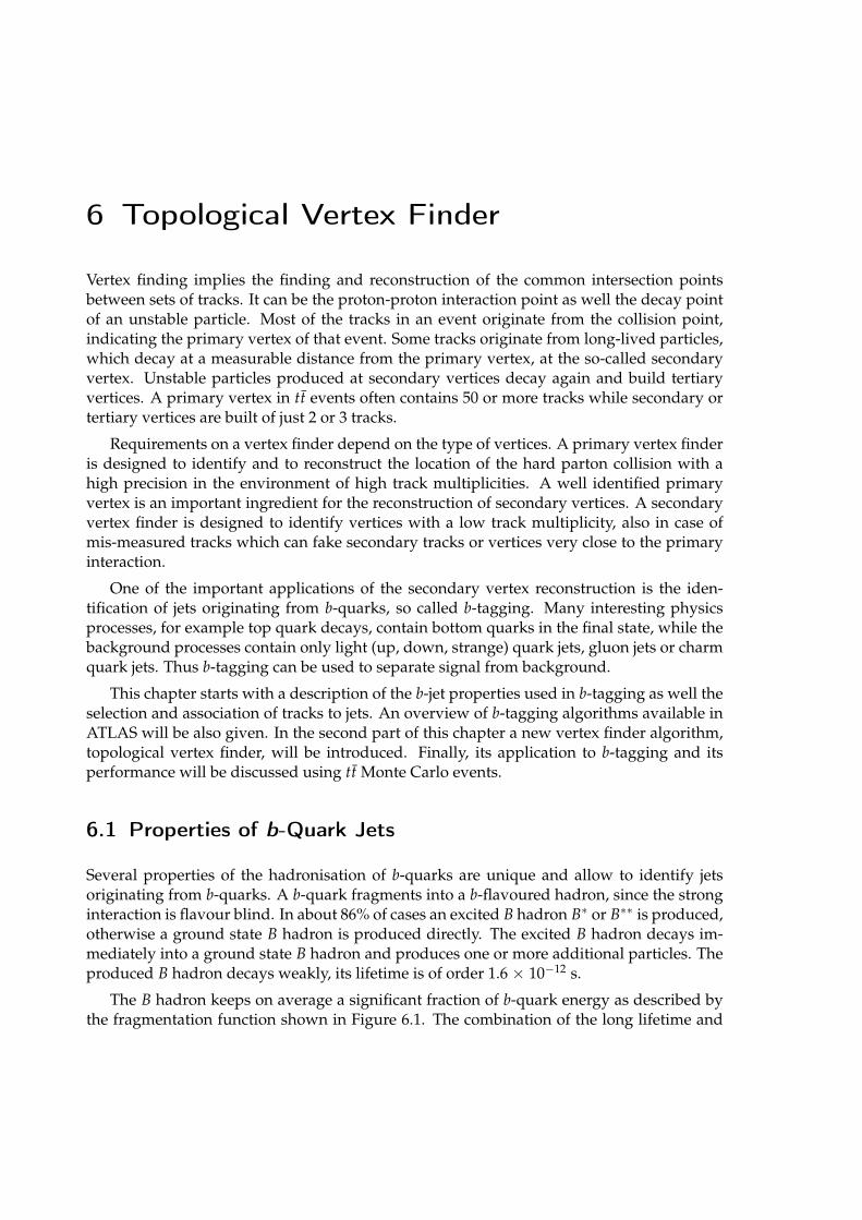
6 Topological Vertex Finder
Vertex finding implies the finding and reconstruction of the common intersection pointsbetween sets of tracks. It can be the proton-proton interaction point as well the decay pointof an unstable particle. Most of the tracks in an event originate from the collision point,indicating the primary vertex of that event. Some tracks originate from long-lived particles,which decay at a measurable distance from the primary vertex, at the so-called secondaryvertex. Unstable particles produced at secondary vertices decay again and build tertiaryvertices. A primary vertex in tt events often contains 50 or more tracks while secondary ortertiary vertices are built of just 2 or 3 tracks.
Requirements on a vertex finder depend on the type of vertices. A primary vertex finderis designed to identify and to reconstruct the location of the hard parton collision with ahigh precision in the environment of high track multiplicities. A well identified primaryvertex is an important ingredient for the reconstruction of secondary vertices. A secondaryvertex finder is designed to identify vertices with a low track multiplicity, also in case ofmis-measured tracks which can fake secondary tracks or vertices very close to the primaryinteraction.
One of the important applications of the secondary vertex reconstruction is the iden-tification of jets originating from b-quarks, so called b-tagging. Many interesting physicsprocesses, for example top quark decays, contain bottom quarks in the final state, while thebackground processes contain only light (up, down, strange) quark jets, gluon jets or charmquark jets. Thus b-tagging can be used to separate signal from background.
This chapter starts with a description of the b-jet properties used in b-tagging as well theselection and association of tracks to jets. An overview of b-tagging algorithms available inATLAS will be also given. In the second part of this chapter a new vertex finder algorithm,topological vertex finder, will be introduced. Finally, its application to b-tagging and itsperformance will be discussed using tt Monte Carlo events.
6.1 Properties of b-Quark Jets
Several properties of the hadronisation of b-quarks are unique and allow to identify jetsoriginating from b-quarks. A b-quark fragments into a b-flavoured hadron, since the stronginteraction is flavour blind. In about 86% of cases an excited B hadron B∗ or B∗∗ is produced,otherwise a ground state B hadron is produced directly. The excited B hadron decays im-mediately into a ground state B hadron and produces one or more additional particles. Theproduced B hadron decays weakly, its lifetime is of order 1.6 × 10⁻¹² s.
The B hadron keeps on average a significant fraction of b-quark energy as described bythe fragmentation function shown in Figure 6.1. The combination of the long lifetime and
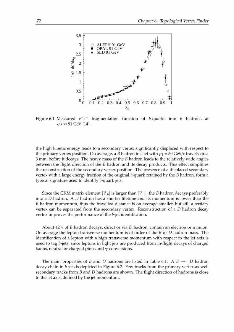
72 Chapter 6. Topological Vertex Finder
0
0.5
1
1.5
2
2.5
3
3.5
0 0.1 0.2 0.3 0.4 0.5 0.6 0.7 0.8 0.9 1xB
1/σ
dσ/
dxB
ALEPH 91 GeVOPAL 91 GeVSLD 91 GeV
Figure 6.1: Measured e+e− fragmentation function of b-quarks into B hadrons at√s ≈ 91 GeV [14].
the high kinetic energy leads to a secondary vertex significantly displaced with respect tothe primary vertex position. On average, a B hadron in a jet with pT = 50 GeV/c travels circa3 mm, before it decays. The heavy mass of the B hadron leads to the relatively wide anglesbetween the flight direction of the B hadron and its decay products. This effect simplifiesthe reconstruction of the secondary vertex position. The presence of a displaced secondaryvertex with a large energy fraction of the original b-quark retained by the B hadron, form atypical signature used to identify b-quark jets.
Since the CKM matrix element |Vcb| is larger than |Vub|, the B hadron decays preferablyinto a D hadron. A D hadron has a shorter lifetime and its momentum is lower than theB hadron momentum, thus the travelled distance is on average smaller, but still a tertiaryvertex can be separated from the secondary vertex. Reconstruction of a D hadron decayvertex improves the performance of the b-jet identification.
About 42% of B hadron decays, direct or via D hadron, contain an electron or a muon.On average the lepton transverse momentum is of order of the B or D hadron mass. Theidentification of a lepton with a high transverse momentum with respect to the jet axis isused to tag b-jets, since leptons in light jets are produced from in-flight decays of chargedkaons, neutral or charged pions and γ-conversions.
The main properties of B and D hadrons are listed in Table 6.1. A B → D hadrondecay chain in b-jets is depicted in Figure 6.2. Few tracks from the primary vertex as wellsecondary tracks from B and D hadrons are shown. The flight direction of hadrons is closeto the jet axis, defined by the jet momentum.
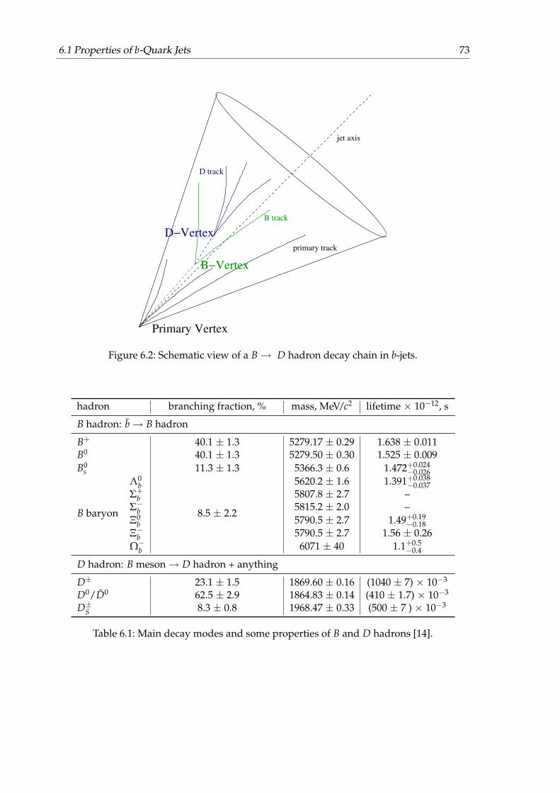
6.1 Properties of b-Quark Jets 73
B−Vertex
Primary Vertex
D−Vertex
primary track
B track
D track
jet axis
Figure 6.2: Schematic view of a B→ D hadron decay chain in b-jets.
hadron branching fraction, % mass, MeV/c2 lifetime × 10−12, s
B hadron: b→ B hadron
B+ 40.1 ± 1.3 5279.17 ± 0.29 1.638 ± 0.011B0 40.1 ± 1.3 5279.50 ± 0.30 1.525 ± 0.009B0
s 11.3 ± 1.3 5366.3 ± 0.6 1.472+0.024−0.026
B baryon
Λ0b
8.5 ± 2.2
5620.2 ± 1.6 1.391+0.038−0.037
Σ+b 5807.8 ± 2.7 –
Σ−b 5815.2 ± 2.0 –Ξ0
b 5790.5 ± 2.7 1.49+0.19−0.18
Ξ−b 5790.5 ± 2.7 1.56 ± 0.26Ω−b 6071 ± 40 1.1+0.5
−0.4
D hadron: B meson→ D hadron + anything
D± 23.1 ± 1.5 1869.60 ± 0.16 (1040 ± 7) × 10−3
D0/D0 62.5 ± 2.9 1864.83 ± 0.14 (410 ± 1.7) × 10−3
D±S 8.3 ± 0.8 1968.47 ± 0.33 (500 ± 7 ) × 10−3
Table 6.1: Main decay modes and some properties of B and D hadrons [14].
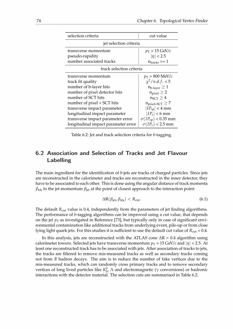
74 Chapter 6. Topological Vertex Finder
selection criteria cut value
jet selection criteria
transverse momentum pT > 15 GeV/cpseudo-rapidity |η| < 2.5number associated tracks ntracks >= 1
track selection criteria
transverse momentum pT > 800 MeV/ctrack fit quality χ2/n.d. f . < 5number of b-layer hits nb-layer ≥ 1number of pixel detector hits npixel ≥ 2number of SCT hits nSCT ≥ 4number of pixel + SCT hits npixel+SCT ≥ 7transverse impact parameter |IPrφ| < 4 mmlongitudinal impact parameter |IPz| < 6 mmtransverse impact parameter error σ(IPrφ) < 0.35 mmlongitudinal impact parameter error σ(IPz) < 2.5 mm
Table 6.2: Jet and track selection criteria for b-tagging.
6.2 Association and Selection of Tracks and Jet FlavourLabelling
The main ingredient for the identification of b-jets are tracks of charged particles. Since jetsare reconstructed in the calorimeter and tracks are reconstructed in the inner detector, theyhave to be associated to each other. This is done using the angular distance of track momenta~ptrk to the jet momentum ~pjet at the point of closest approach to the interaction point:
∆R(~pjet,~ptrk) < Rcut. (6.1)
The default Rcut value is 0.4, independently from the parameters of jet finding algorithms.The performance of b-tagging algorithms can be improved using a cut value, that dependson the jet pT as investigated in Reference [73], but typically only in case of significant envi-ronmental contamination like additional tracks from underlying event, pile-up or from closelying light quark jets. For this studies it is sufficient to use the default cut value of Rcut = 0.4.
In this analysis, jets are reconstructed with the ATLAS cone ∆R = 0.4 algorithm usingcalorimeter towers. Selected jets have transverse momentum pT > 15 GeV/c and |η| < 2.5. Atleast one reconstructed track has to be associated with jets. After association of tracks to jets,the tracks are filtered to remove mis-measured tracks as well as secondary tracks comingnot from B hadron decays. The aim is to reduce the number of fake vertices due to themis-measured tracks, which can randomly cross primary tracks and to remove secondaryvertices of long lived particles like K0
S, Λ and electromagnetic (γ conversions) or hadronicinteractions with the detector material. The selection cuts are summarised in Table 6.2.

6.2 Association and Selection of Tracks and Jet Flavour Labelling 75
(a) track transverse momentum
(b) track transverse impact parameter (c) track longitudinal impact parameter
Figure 6.3: Transverse momentum distributions of tracks associated to light and b-jets (a).Transverse (b) and longitudinal (c) impact parameter distributions of tracks asso-ciated to b-jets. Tracks are subdivided into categories according to their physicalorigin.
To reduce the number of tracks from long lived particles or from material interactionsin the detector, at least one hit in the first layer of the pixel detector is required. The mea-surement in the first layer is also crucial for the resolution of the vertex position. To fitrequirements on track quality, a minimum number of hits in the pixel and SCT detectors arerequired. Track fit quality divided by the number of degrees of freedom should be χ2/n.d. f .< 5. As already mentioned in the previous section B hadrons keep about 70% of the originalb-quark energy. In b-jets the transverse momentum of B hadron decay products is on aver-age higher than for tracks originating from the b-quark fragmentation as shown in Figure
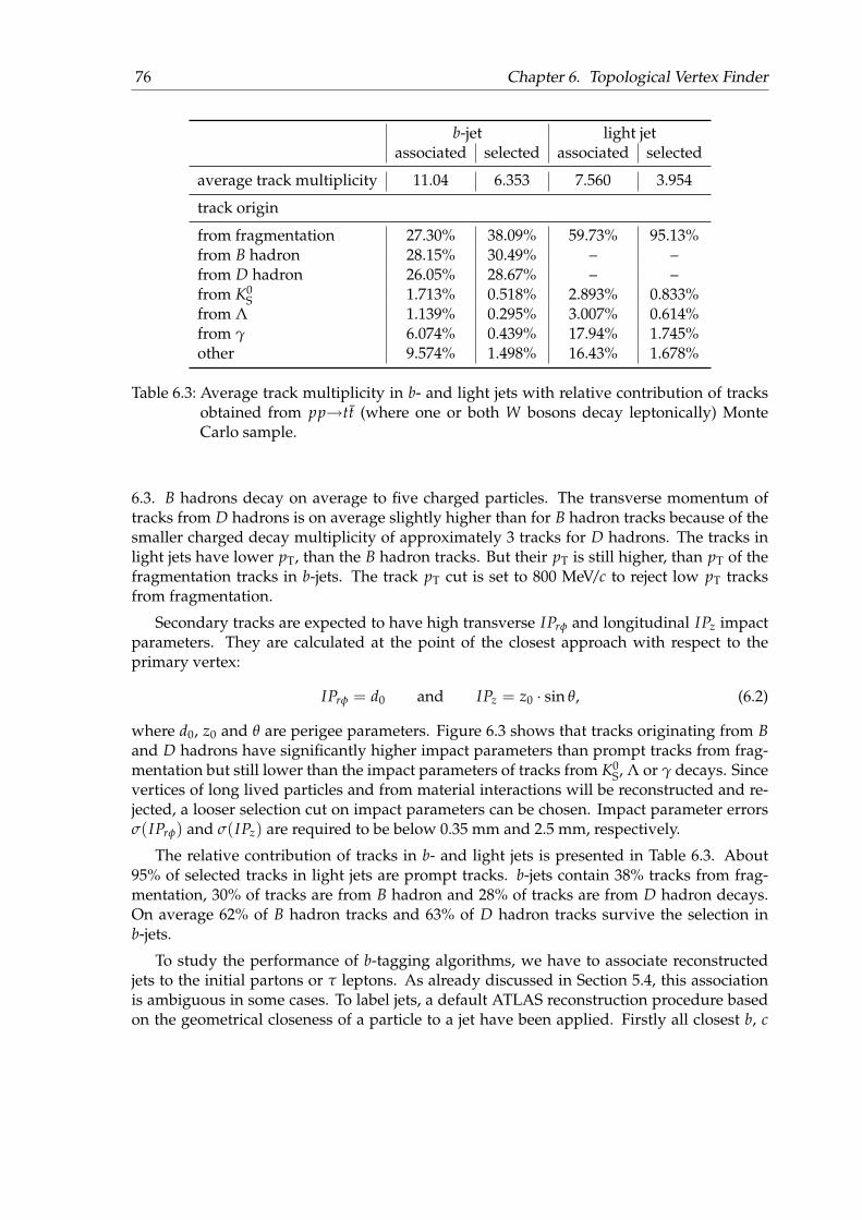
76 Chapter 6. Topological Vertex Finder
b-jet light jetassociated selected associated selected
average track multiplicity 11.04 6.353 7.560 3.954
track origin
from fragmentation 27.30% 38.09% 59.73% 95.13%from B hadron 28.15% 30.49% – –from D hadron 26.05% 28.67% – –from K0
S 1.713% 0.518% 2.893% 0.833%from Λ 1.139% 0.295% 3.007% 0.614%from γ 6.074% 0.439% 17.94% 1.745%other 9.574% 1.498% 16.43% 1.678%
Table 6.3: Average track multiplicity in b- and light jets with relative contribution of tracksobtained from pp→tt (where one or both W bosons decay leptonically) MonteCarlo sample.
6.3. B hadrons decay on average to five charged particles. The transverse momentum oftracks from D hadrons is on average slightly higher than for B hadron tracks because of thesmaller charged decay multiplicity of approximately 3 tracks for D hadrons. The tracks inlight jets have lower pT, than the B hadron tracks. But their pT is still higher, than pT of thefragmentation tracks in b-jets. The track pT cut is set to 800 MeV/c to reject low pT tracksfrom fragmentation.
Secondary tracks are expected to have high transverse IPrφ and longitudinal IPz impactparameters. They are calculated at the point of the closest approach with respect to theprimary vertex:
IPrφ = d0 and IPz = z0 · sin θ, (6.2)
where d0, z0 and θ are perigee parameters. Figure 6.3 shows that tracks originating from Band D hadrons have significantly higher impact parameters than prompt tracks from frag-mentation but still lower than the impact parameters of tracks from K0
S, Λ or γ decays. Sincevertices of long lived particles and from material interactions will be reconstructed and re-jected, a looser selection cut on impact parameters can be chosen. Impact parameter errorsσ(IPrφ) and σ(IPz) are required to be below 0.35 mm and 2.5 mm, respectively.
The relative contribution of tracks in b- and light jets is presented in Table 6.3. About95% of selected tracks in light jets are prompt tracks. b-jets contain 38% tracks from frag-mentation, 30% of tracks are from B hadron and 28% of tracks are from D hadron decays.On average 62% of B hadron tracks and 63% of D hadron tracks survive the selection inb-jets.
To study the performance of b-tagging algorithms, we have to associate reconstructedjets to the initial partons or τ leptons. As already discussed in Section 5.4, this associationis ambiguous in some cases. To label jets, a default ATLAS reconstruction procedure basedon the geometrical closeness of a particle to a jet have been applied. Firstly all closest b, c
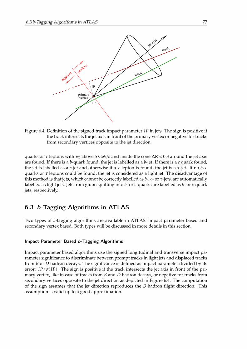
6.3 b-Tagging Algorithms in ATLAS 77
IP
IP
primaryvertex
jet ax
is
track
trackpositiv
e
negat
ive
Figure 6.4: Definition of the signed track impact parameter IP in jets. The sign is positive ifthe track intersects the jet axis in front of the primary vertex or negative for tracksfrom secondary vertices opposite to the jet direction.
quarks or τ leptons with pT above 5 GeV/c and inside the cone ∆R < 0.3 around the jet axisare found. If there is a b-quark found, the jet is labelled as a b-jet. If there is a c quark found,the jet is labelled as a c-jet and otherwise if a τ lepton is found, the jet is a τ-jet. If no b, cquarks or τ leptons could be found, the jet is considered as a light jet. The disadvantage ofthis method is that jets, which cannot be correctly labelled as b-, c- or τ-jets, are automaticallylabelled as light jets. Jets from gluon splitting into b- or c-quarks are labelled as b- or c-quarkjets, respectively.
6.3 b-Tagging Algorithms in ATLAS
Two types of b-tagging algorithms are available in ATLAS: impact parameter based andsecondary vertex based. Both types will be discussed in more details in this section.
Impact Parameter Based b-Tagging Algorithms
Impact parameter based algorithms use the signed longitudinal and transverse impact pa-rameter significance to discriminate between prompt tracks in light jets and displaced tracksfrom B or D hadron decays. The significance is defined as impact parameter divided by itserror: IP/σ(IP). The sign is positive if the track intersects the jet axis in front of the pri-mary vertex, like in case of tracks from B and D hadron decays, or negative for tracks fromsecondary vertices opposite to the jet direction as depicted in Figure 6.4. The computationof the sign assumes that the jet direction reproduces the B hadron flight direction. Thisassumption is valid up to a good approximation.
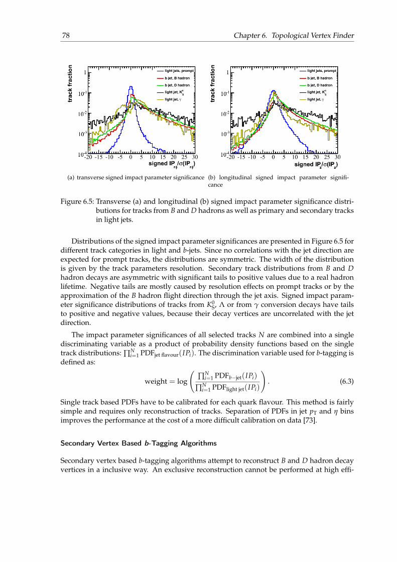
78 Chapter 6. Topological Vertex Finder
(a) transverse signed impact parameter significance (b) longitudinal signed impact parameter signifi-cance
Figure 6.5: Transverse (a) and longitudinal (b) signed impact parameter significance distri-butions for tracks from B and D hadrons as well as primary and secondary tracksin light jets.
Distributions of the signed impact parameter significances are presented in Figure 6.5 fordifferent track categories in light and b-jets. Since no correlations with the jet direction areexpected for prompt tracks, the distributions are symmetric. The width of the distributionis given by the track parameters resolution. Secondary track distributions from B and Dhadron decays are asymmetric with significant tails to positive values due to a real hadronlifetime. Negative tails are mostly caused by resolution effects on prompt tracks or by theapproximation of the B hadron flight direction through the jet axis. Signed impact param-eter significance distributions of tracks from K0
S, Λ or from γ conversion decays have tailsto positive and negative values, because their decay vertices are uncorrelated with the jetdirection.
The impact parameter significances of all selected tracks N are combined into a singlediscriminating variable as a product of probability density functions based on the singletrack distributions: ∏N
i=1 PDFjet flavour(IPi). The discrimination variable used for b-tagging isdefined as:
weight = log
(∏N
i=1 PDFb−jet(IPi)
∏Ni=1 PDFlight jet(IPi)
). (6.3)
Single track based PDFs have to be calibrated for each quark flavour. This method is fairlysimple and requires only reconstruction of tracks. Separation of PDFs in jet pT and η binsimproves the performance at the cost of a more difficult calibration on data [73].
Secondary Vertex Based b-Tagging Algorithms
Secondary vertex based b-tagging algorithms attempt to reconstruct B and D hadron decayvertices in a inclusive way. An exclusive reconstruction cannot be performed at high effi-

6.3 b-Tagging Algorithms in ATLAS 79
ciency due to a huge number of different decay modes, missing tracks of neutral particlesand limited detector resolution.
Even the inclusive secondary vertex reconstruction is a challenging task: the averagenumber of reconstructed and selected secondary tracks from B/D hadrons is below 2, asevaluated in Table 6.3. Decays of hadrons close to the primary vertex are difficult to sepa-rate from the primary interaction and they cannot be considered for the secondary vertexreconstruction. The probability to distinguish between B and D hadron vertices dependsstrongly on the distance between the vertices and on the track parameters resolution. Espe-cially at low track momenta, the resolution is not sufficient to separate both vertices.
The VKalVrt [117] reconstruction package implemented in the ATLAS software frame-work attempts to reconstruct a single secondary vertex. It starts with the selected tracksassociated to a jet and forms a “two-track” vertex from all possible combinations of twotracks, which satisfy following selection criteria:
• the impact parameter significance of each track is larger than 2 and the sum of thesetwo significances is larger than 6
• the probability of the vertex fit, based on χ2 of the fit, is > 3.5%
• “two-track” vertices~r2tr are required to be produced in the b-jet direction, ~pjet, by re-quiring the scalar product (~r2tr −~rprimary) · ~pjet to be positive, where~rprimary is the po-sition of the primary vertex
• “two-track” vertices compatible with K0S Λ, γ decays or with material interactions are
rejected
All tracks from the accepted two-track vertices are used to fit a single secondary vertex. Ifthe resulting vertex has a χ2 above χ2
max, the track with the highest contribution is removedand the vertex fit is redone. This procedure is repeated until a χ2 < χ2
max is obtained.
Properties of the reconstructed secondary vertex are used in the b-tagging algorithmBTagVrtSec [118] to separate light and b-jets. The presence of a reconstructed vertex in thejet itself is the first variable, because the probability to find a secondary vertex in b-jets issignificantly higher for b-jets than for light jets. The mass of the reconstructed vertex M,the ratio of the energy of charged particle tracks at vertex to the total energy of all chargedparticles R and the number of accepted “two-track” vertices N are also used. The distancebetween primary and secondary vertices is only used if the tagger is not combined with aimpact parameter based tagger. These variables are transformed to facilitate the calibrationof the b-tagging algorithm on data and to reduce the necessary amount of data:
• transformed invariant mass: M′ = MM+1
• transformed energy ratio: R′ = R0.7
• transformed number of accepted “two-track” secondary vertices: N′ = log N
The probability density function is defined as:
PDF = (1− ε) · δ(M′, R′, N′) + ε ·ASH(M′, R′, N′), (6.4)
where ε is the secondary vertex reconstruction efficiency and δ(M′, R′, N′) is a δ-functionto account for a less than 100% efficient reconstruction. A continuous probability density
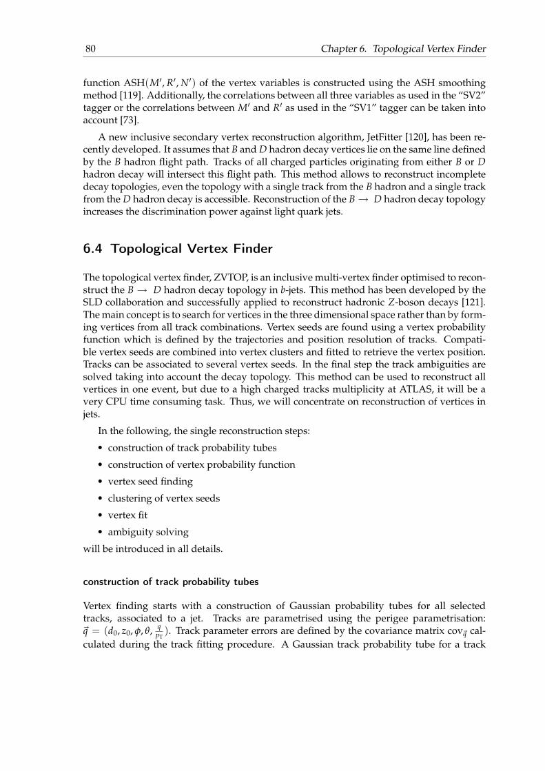
80 Chapter 6. Topological Vertex Finder
function ASH(M′, R′, N′) of the vertex variables is constructed using the ASH smoothingmethod [119]. Additionally, the correlations between all three variables as used in the “SV2”tagger or the correlations between M′ and R′ as used in the “SV1” tagger can be taken intoaccount [73].
A new inclusive secondary vertex reconstruction algorithm, JetFitter [120], has been re-cently developed. It assumes that B and D hadron decay vertices lie on the same line definedby the B hadron flight path. Tracks of all charged particles originating from either B or Dhadron decay will intersect this flight path. This method allows to reconstruct incompletedecay topologies, even the topology with a single track from the B hadron and a single trackfrom the D hadron decay is accessible. Reconstruction of the B→ D hadron decay topologyincreases the discrimination power against light quark jets.
6.4 Topological Vertex Finder
The topological vertex finder, ZVTOP, is an inclusive multi-vertex finder optimised to recon-struct the B → D hadron decay topology in b-jets. This method has been developed by theSLD collaboration and successfully applied to reconstruct hadronic Z-boson decays [121].The main concept is to search for vertices in the three dimensional space rather than by form-ing vertices from all track combinations. Vertex seeds are found using a vertex probabilityfunction which is defined by the trajectories and position resolution of tracks. Compati-ble vertex seeds are combined into vertex clusters and fitted to retrieve the vertex position.Tracks can be associated to several vertex seeds. In the final step the track ambiguities aresolved taking into account the decay topology. This method can be used to reconstruct allvertices in one event, but due to a high charged tracks multiplicity at ATLAS, it will be avery CPU time consuming task. Thus, we will concentrate on reconstruction of vertices injets.
In the following, the single reconstruction steps:
• construction of track probability tubes
• construction of vertex probability function
• vertex seed finding
• clustering of vertex seeds
• vertex fit
• ambiguity solving
will be introduced in all details.
construction of track probability tubes
Vertex finding starts with a construction of Gaussian probability tubes for all selectedtracks, associated to a jet. Tracks are parametrised using the perigee parametrisation:~q = (d0, z0, φ, θ, q
pT). Track parameter errors are defined by the covariance matrix cov~q cal-
culated during the track fitting procedure. A Gaussian track probability tube for a track
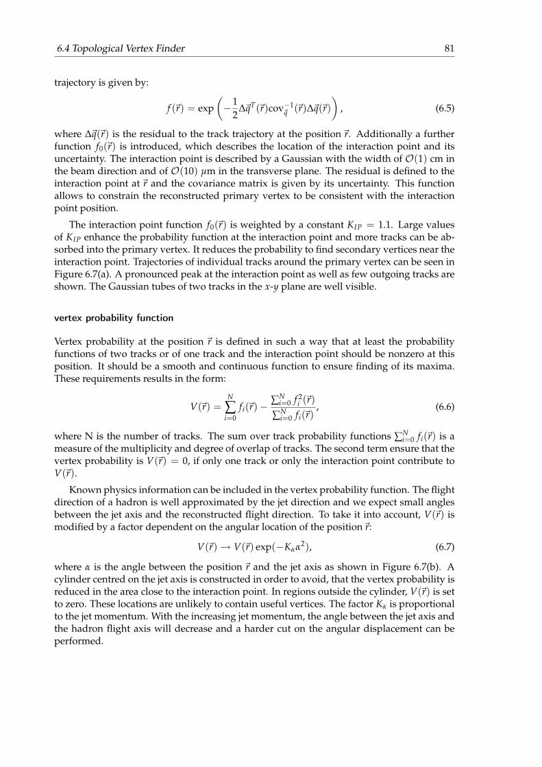
6.4 Topological Vertex Finder 81
trajectory is given by:
f (~r) = exp(−1
2∆~qT(~r)cov−1
~q (~r)∆~q(~r))
, (6.5)
where ∆~q(~r) is the residual to the track trajectory at the position~r. Additionally a furtherfunction f0(~r) is introduced, which describes the location of the interaction point and itsuncertainty. The interaction point is described by a Gaussian with the width of O(1) cm inthe beam direction and of O(10) µm in the transverse plane. The residual is defined to theinteraction point at ~r and the covariance matrix is given by its uncertainty. This functionallows to constrain the reconstructed primary vertex to be consistent with the interactionpoint position.
The interaction point function f0(~r) is weighted by a constant KIP = 1.1. Large valuesof KIP enhance the probability function at the interaction point and more tracks can be ab-sorbed into the primary vertex. It reduces the probability to find secondary vertices near theinteraction point. Trajectories of individual tracks around the primary vertex can be seen inFigure 6.7(a). A pronounced peak at the interaction point as well as few outgoing tracks areshown. The Gaussian tubes of two tracks in the x-y plane are well visible.
vertex probability function
Vertex probability at the position ~r is defined in such a way that at least the probabilityfunctions of two tracks or of one track and the interaction point should be nonzero at thisposition. It should be a smooth and continuous function to ensure finding of its maxima.These requirements results in the form:
V(~r) =N
∑i=0
fi(~r)−∑N
i=0 f 2i (~r)
∑Ni=0 fi(~r)
, (6.6)
where N is the number of tracks. The sum over track probability functions ∑Ni=0 fi(~r) is a
measure of the multiplicity and degree of overlap of tracks. The second term ensure that thevertex probability is V(~r) = 0, if only one track or only the interaction point contribute toV(~r).
Known physics information can be included in the vertex probability function. The flightdirection of a hadron is well approximated by the jet direction and we expect small anglesbetween the jet axis and the reconstructed flight direction. To take it into account, V(~r) ismodified by a factor dependent on the angular location of the position~r:
V(~r)→ V(~r) exp(−Kαα2), (6.7)
where α is the angle between the position ~r and the jet axis as shown in Figure 6.7(b). Acylinder centred on the jet axis is constructed in order to avoid, that the vertex probability isreduced in the area close to the interaction point. In regions outside the cylinder, V(~r) is setto zero. These locations are unlikely to contain useful vertices. The factor Kα is proportionalto the jet momentum. With the increasing jet momentum, the angle between the jet axis andthe hadron flight axis will decrease and a harder cut on the angular displacement can beperformed.
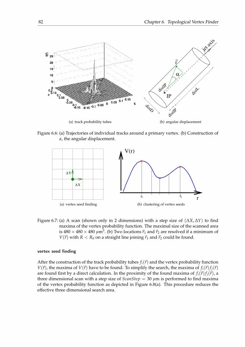
82 Chapter 6. Topological Vertex Finder
(a) track probability tubes
jet a
xis
distIP
dist
L
distD
IP
α
distIP
r
(b) angular displacement
Figure 6.6: (a) Trajectories of individual tracks around a primary vertex. (b) Construction ofα, the angular displacement.
∆X
Y∆
(a) vertex seed finding
rr r21
V(r)
(b) clustering of vertex seeds
Figure 6.7: (a) A scan (shown only in 2 dimensions) with a step size of (∆X, ∆Y) to findmaxima of the vertex probability function. The maximal size of the scanned areais 480× 480× 480 µm3. (b) Two locations~r1 and~r2 are resolved if a minimum ofV(~r) with R < R0 on a straight line joining~r1 and~r2 could be found.
vertex seed finding
After the construction of the track probability tubes fi(~r) and the vertex probability functionV(~r), the maxima of V(~r) have to be found. To simplify the search, the maxima of fi(~r) f j(~r)are found first by a direct calculation. In the proximity of the found maxima of fi(~r) f j(~r), athree dimensional scan with a step size of ScanStep = 30 µm is performed to find maximaof the vertex probability function as depicted in Figure 6.8(a). This procedure reduces theeffective three dimensional search area.

6.4 Topological Vertex Finder 83
clustering of vertex seeds
Found vertex seeds have to be clustered together to form vertex candidates. Two vertexseeds are resolved, if a minimum of V(~r) could be found between these two locations asshown in Figure 6.8(b). The absolute value of the minimum should depend on the valueof the vertex probability function of both seeds and this leads to the following resolutioncriterion. Two locations~r1 and~r2 are resolved if:
minV(~r) :~r ∈~r1 + α(~r2 −~r1), 0 ≤ α ≤ 1minV(~r1), V(~r2)
< R0, (6.8)
where the numerator is the minimum of V(~r) on a straight line joining ~r1 and ~r2 and thedenominator is the lower of the two vertex probabilities. V(~r) is determined for a finitenumber of points Nstep = 16 on this line. The number of steps can be smaller, if the step sizeis below a certain minimal length, min Lstep = 15µm. The number of found vertices dependson the cut value R0, the default value is set to R0 = 0.6.
vertex fit
The clustered vertex candidates are fitted in order to calculate vertex positions and theirerrors. Used vertex fitter is based on the Billoir vertex fitting technique [122]. Vertex clusterswith the two dimensional distance significance dist2D/σ(dist2D) below signi f 2D = 2 arecompatible with the interaction point position. This cluster is labeled as “primary” andfitted using the interaction point constraint. Tracks with a large contribution to the χ2 of thevertex fit are iteratively removed. The fitting and track removal procedure continue, till atleast two tracks remain. If χ2 of the vertex candidate is still above a threshold χ2
max = 7, thisvertex candidate will be dropped. The vertex candidate is rejected if the number of tracksis less than two, except for the primary vertex, which can have only one associated trackbecause of the interaction point constraint.
Vertex candidates with two associated tracks may be produced through hadronic inter-actions in the inner detector, K0
S and Λ decays or γ conversions. If tracks have oppositecharges, the invariant mass at vertex is calculated using (p,π), (π,π) and (e,e) mass hypothe-ses for the tracks. The invariant mass distributions m(π, π) and m(p, π) are presented inFigure 6.9(a) and 6.9(b), respectively. Sharp peaks at mK0
S≈ 500 MeV/c2 and at mΛ ≈
1116 MeV/c2 are visible in particular for light jets. The fraction of Λ baryons in b-jets isnegligible.
A neutral particle is reconstructed out of both charged tracks and its signed three di-mensional impact parameter significance is calculated with respect to the primary vertex.The distributions of the signed impact parameter significances are shown in 6.9(d). K0
S andΛ particle candidates in light jets are expected to be produced at primary vertex, thus theywill have small impact parameters significances, signi f Neutral < 2. All two track verticeswithin the K0
S or Λ particle mass window and compatible with the primary vertex as well asvertices within the γ mass window are rejected.
In Figure 6.9(c) secondary vertices produced through material interactions in the detectorare clearly visible around 50 mm at the position of the first layer. A small peak can be seen

84 Chapter 6. Topological Vertex Finder
Figure 6.8: Reconstructed “two-track” vertices from K0S (a), Λ (b) decays and material inter-
actions (c) in light and b-jets. The proton mass is assigned to the track with thelargest momentum. (d) Signed impact parameter significance of K0
S candidatesselected in the K0
S mass window.
around 30 mm, at the position of the beam pipe. Such vertices are rejected, if the distancedifference to the beam pipe walls is ∆RBP < 1 mm or to the layers of the inner detector∆RBlay < 3.5 mm.
ambiguity solving
In general each track can be associated with more than one vertex candidate. It enhancesthe vertex finding efficiency, but these ambiguities will be resolved in the last step. Thefollowing procedure, presented in Figure 6.9, is applied to solve the ambiguities. All se-lected vertex candidates are sorted according to their three dimensional distance from theinteraction point. The tracks associated to the furtherst vertex are fixed in that vertex andremoved from any others. Vertices with removed tracks are refitted and the distance to the

6.5 Secondary Vertex Reconstruction Performance 85
track 1track 2
track 3track 4
track 5
vertex 1
vertex 2
vertex 3
vertex 4
vertex 5
vertex 6
(a) step 1
track 1track 2
track 3track 4
track 5
vertex 1
vertex 4
vertex 5
vertex 6
(b) step 2
track 1track 2
track 3track 4
track 5
vertex 1
vertex 4
vertex 6
(c) step 3
Figure 6.9: Ambiguity solving procedure: (a) association of tracks 1 and 2 to vertex 1, re-moval of these tracks from vertex 2 and 3, vertices 2 and 3 are rejected; (b) associ-ation of tracks 3 and 4 to the vertex 4, removal from vertex 5; vertex 5 is rejected;(c) final association.
interaction point is recalculated again. The remaining vertices are considered in order ofdecreasing distances and the procedure is repeated again till all ambiguities are solved.
This procedure allows to associate compatible tracks with the D hadron vertex at first, inthe second step with the B hadron vertex and in the final step with the primary vertex. If theopening angle between decaying particles is very small, the tracks of decay products can beassociated to the decay vertex as well to the production vertex of the decaying particle. The“outside-inside” ambiguity solving procedure provides an optimal solution in such cases.
All discussed tunable parameter of topological vertex finder and corresponding defaultvalues optimised to reconstruct secondary vertices in tt events are listed in Table 6.4.
6.5 Secondary Vertex Reconstruction Performance
The performance of the topological vertex finder will be discussed in this section. The mainpoint of interest is the secondary vertex reconstruction efficiency and purity in light and b-jets. The performance of ZVTOP vertex finder will be compared with the performance of theinclusive secondary vertex finder VKalVrt using jets reconstructed in tt Monte Carlo events.
Reconstructed vertices are labeled as secondary vertices, if their three dimensional flightlength significance dist3D/σ(dist3D) is above 3.5. Secondary vertex reconstruction efficiency
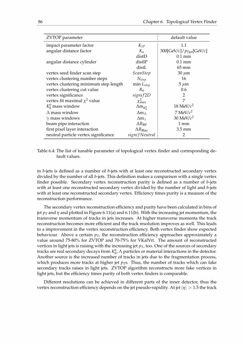
86 Chapter 6. Topological Vertex Finder
ZVTOP parameter default value
impact parameter factor KIP 1.1angular distance factor Kα 300[GeV/c]/pTjet[GeV/c]
angular distance cylinderdistD 0.1 mmdistIP 0.1 mmdistL 65 mm
vertex seed finder scan step ScanStep 30 µmvertex clustering number steps Nstep 16vertex clustering minimum step length min Lstep 5 µmvertex clustering cut value R0 0.6vertex significance signi f 2D 2vertex fit maximal χ2 value χ2
max 7K0
S mass window ∆mK0S
18 MeV/c2
Λ mass window ∆mΛ 7 MeV/c2
γ mass windows ∆mγ 30 MeV/c2
beam pipe interaction ∆RBP 1 mmfirst pixel layer interaction ∆RBlay 3.5 mmneutral particle vertex significance signi f Neutral 2
Table 6.4: The list of tunable parameter of topological vertex finder and corresponding de-fault values.
in b-jets is defined as a number of b-jets with at least one reconstructed secondary vertexdivided by the number of all b-jets. This definition makes a comparison with a single vertexfinder possible. Secondary vertex reconstruction purity is defined as a number of b-jetswith at least one reconstructed secondary vertex divided by the number of light and b-jetswith at least one reconstructed secondary vertex. Efficiency times purity is a measure of thereconstruction performance.
The secondary vertex reconstruction efficiency and purity have been calculated in bins ofjet pT and η and plotted in Figure 6.11(a) and 6.11(b). With the increasing jet momentum, thetransverse momentum of tracks in jets increases. At higher transverse momenta the trackreconstruction becomes more efficient and the track resolution improves as well. This leadsto a improvement in the vertex reconstruction efficiency. Both vertex finder show expectedbehaviour. Above a certain pT, the reconstruction efficiency approaches approximately avalue around 75-80% for ZVTOP and 70-75% for VKalVrt. The amount of reconstructedvertices in light jets is raising with the increasing jet pT, too. One of the sources of secondarytracks are real secondary decays from K0
S, Λ particles or material interactions in the detector.Another source is the increased number of tracks in jets due to the fragmentation process,which produces more tracks at higher jet pTs. Thus, the number of tracks which can fakesecondary tracks raises in light jets. ZVTOP algorithm reconstructs more fake vertices inlight jets, but the efficiency times purity of both vertex finders is comparable.
Different resolutions can be achieved in different parts of the inner detector, thus thevertex reconstruction efficiency depends on the jet pseudo-rapidity. At jet |η| > 1.5 the track

6.5 Secondary Vertex Reconstruction Performance 87
(a) reconstruction performance versus jet pT
(b) reconstruction performance versus jet η
Figure 6.10: Secondary vertex reconstruction performance versus jet pT (a) and η (b).

88 Chapter 6. Topological Vertex Finder
resolutions get worse and the track reconstruction efficiency drops. The consequence is adecrease in the vertex reconstruction efficiency and an increase of fake vertices.
6.6 Application to b-Tagging
The number of reconstructed secondary vertices and their properties are used to tag b-quarkjets. The b-tagging algorithm is based on a likelihood function build of the following vari-ables:
• number of secondary vertices
• total number of tracks at these vertices
• invariant mass of all charged particle tracks associated to the secondary vertices witha correction for neutral particles
• the sum over the energies of charged particles at vertex divided by the sum of theenergies of all charged particles associated to the jet
• three dimensional flight length significance of the furthest displaced vertex
All variables will be introduced and discussed below. Distributions of these variables arepresented in Figure 6.11 for b-quark and light quark jets in tt events. They are compared tothe distributions retrieved with the VKalVrt reconstruction algorithm as well.
Both secondary vertex finder require secondary vertices with the flight length signifi-cance above 3.5. ZVTOP has a higher secondary vertex reconstruction efficiency of ∼ 70%but also a higher fake rate of ∼ 4% in light jets compared to VKalVrt algorithm (∼ 67% and∼ 2%, respectively).
Secondary vertices in light quark jets contain mostly only two associated tracks. Theaverage number of tracks at secondary vertices in b-quark jets is 3.42 and 3.14 for ZVTOPand VKalVrt, respectively. ZVTOP associates 8% more tracks to secondary vertices in b-quark jets and around 5% more tracks in light quark jets. In Table 6.3 it has been shown thaton average 3.76 tracks from B and D hadrons are expected in the b-quark jets. This numberagrees quite well with the number of tracks associated to the secondary vertices.
The invariant mass at vertex is calculated assuming that each track has the mass of a pion.For the topological vertex finder the mass is partially corrected for the presence of neutralparticles at the B/D hadron decay vertex. If all decay products of hadrons could be detectedand reconstucted, the sum of all momenta at decay vertex ~pvertex would point into the B-flight direction. This property can be used to correct for the missing transverse component ofthe momentum pT,vertex with respect to the flight direction, since the longitudinal componentis not accessible [123]:
mB,corrected =√
m2charged + p2
T,vertex + |pT,vertex|. (6.9)
The invariant mass calculated using only charged track particles distributions is comparablefor both vertex finder apart from the very low and very high mass tails. The K0
S and Λinvariant mass peaks are still visible and can be removed increasing the mass window cut.

6.6 Application to b-Tagging 89
Figure 6.11: Distributions of variables used to tag b-jets: number of reconstucted vertices,number of tracks associated to a vertex, corrected invariant mass at vertex, flightlength significance and energy fraction at vertex for light and b-jets. They arecompared to distributions retrieved with the VKalVrt reconstruction algorithm.The invariant mass without a correction for the neutral tracks is shown for abetter comparison between both vertex finder.

90 Chapter 6. Topological Vertex Finder
The corrected invariant mass distribution is shifted to higher mass values and shows a goodseparation between b- and light quark jets.
ZVTOP reconstructs more secondary vertices with a lower flight length significance, butthe shapes are still well comparable for both vertex finder. The energy fraction at vertexis lower for VKalVrt, because VKalVrt associates on average less charged track particles tovertex than ZVTOP.
As already mentioned, a likelihood function is build out of these variables. The likeli-hood function is defined as a product of the single probability density functions:
Ljet flavour =5
∏i=1
PDFjet flavour(variablei), (6.10)
and the discrimination variable used for b-tagging is logarithm of the ratio of PDFs:
weight = log(
Lb−jet
Llight jet
). (6.11)
Additionally a multilayer perceptron (MLP) neural network (NN) [124] implemented inTMVA [125] have been used. The input layer contains as many neurons as input variablesand one additional neuron, the so-called “bias node”. The output layer contains only asingle neuron for the signal weight used as a discrimination variable for b-tagging. Onlyone hidden layer has been used. All neuron inputs to a layer are linear combinations of theneuron output of the previous layer. The transfer from input to output is performed viaa sigmoid activation function. A detailed information on the NN implementation can befound in Reference [125].
6.7 Performance in Rejecting Light Quark Jets
The performance of the topological vertex finder developed in this thesis will be analysedand compared to the performance of another inclusive secondary vertex based algorithmavailable in ATLAS, BtagSecVtx. Before starting the discussion about the performance ofb-tagging algorithms, two definitions will be introduced: tagging efficiency and rejection.The efficiency to tag a jet of flavour q as b-quark jet, εq is defined as:
εq =number of jets of real flavour q tagged as b
number of jets of real flavour q. (6.12)
εb is called b-tagging efficiency and εuds is mis-tagging rate. The inverse of the mis-taggingrate ruds = 1/εuds is called light quark jet rejection.
The b-tagging efficiency versus the light quark jet rejection rate is ploted in Figure 6.12and the rejection rates for the fixed b-tagging efficiencies of 50%, 60% and 70% are listedin Table 6.5 for different tagging algorithms. The maximum achievable b-tagging efficiencyof secondary vertex based algorithms is limited by the efficiency to reconstruct a displacedvertex.
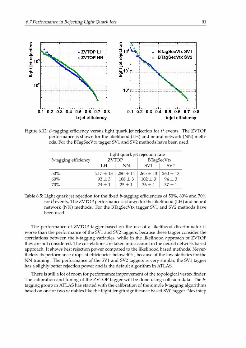
6.7 Performance in Rejecting Light Quark Jets 91
Figure 6.12: B-tagging efficiency versus light quark jet rejection for tt events. The ZVTOPperformance is shown for the likelihood (LH) and neural network (NN) meth-ods. For the BTagSecVtx tagger SV1 and SV2 methods have been used.
b-tagging efficiencylight quark jet rejection rate
ZVTOP BTagSecVtxLH NN SV1 SV2
50% 217 ± 13 280 ± 14 265 ± 13 260 ± 1360% 92 ± 3 108 ± 3 102 ± 3 94 ± 370% 24 ± 1 25 ± 1 36 ± 1 37 ± 1
Table 6.5: Light quark jet rejection for the fixed b-tagging efficiencies of 50%, 60% and 70%for tt events. The ZVTOP performance is shown for the likelihood (LH) and neuralnetwork (NN) methods. For the BTagSecVtx tagger SV1 and SV2 methods havebeen used.
The performance of ZVTOP tagger based on the use of a likelihood discriminator isworse than the performance of the SV1 and SV2 taggers, because these tagger consider thecorrelations between the b-tagging variables, while in the likelihood approach of ZVTOPthey are not considered. The correlations are taken into account in the neural network basedapproach. It shows best rejection power compared to the likelihood based methods. Never-theless its performance drops at efficiencies below 40%, because of the low statistics for theNN training. The performance of the SV1 and SV2 taggers is very similar, the SV1 taggerhas a slighly better rejection power and is the default algorithm in ATLAS.
There is still a lot of room for performance improvement of the topological vertex finder.The calibration and tuning of the ZVTOP tagger will be done using collision data. The b-tagging group in ATLAS has started with the calibration of the simple b-tagging algorithmsbased on one or two variables like the flight length significance based SV0 tagger. Next step

92 Chapter 6. Topological Vertex Finder
will be more complex but also more powerful tagger: BTagSecVtx, JetFitter, ZVTOP or alsoimpact parameter based tagger.
7 The tt Invariant Mass Distribution
This analysis is based on a model independent search of a narrow width resonance in thesemi-leptonic decay channel of the top quark pairs. First direct searches for resonant tt pro-duction have been done at the TEVATRON. So far no significant deviation from the StandardModel predictions could be observed. A higher centre-of-mass energy at the LHC allows toextend these searches for the first time into the TeV-regime.
The production cross-section of the new heavy particles is very low compared to theStandard Model tt pair production. We will focus on the efficient selection and identifica-tion of signal events in the whole accessible mtt-range. The topology of events produced atthe tt mass threshold differs strongly from the event topology at a few TeV. A new recon-struction scheme has been developed to deal with the different topologies. In this chapterwe start with the discussion of the semi-leptonic event selection and identification of theevent topology at different resonance masses. Based on it, an analysis strategy will be de-veloped and the performance of the reconstruction algorithm will be discussed. Finally theexpected systematical uncertainties will be given.
7.1 Event Selection
The tt final state is quite complex. The top quarks decay to nearly 100% in a W boson and abottom quark. The W boson decays into a lepton and neutrino pair or in a quark anti-quarkpair. Requiring semi-leptonic tt decays, we expect exactly one lepton, missing transverse en-ergy due to the escaping neutrino and jets. The decay products should have high transversemomenta, because the mass of the resonance particles is of the order of several top quarkmasses. We consider only reconstructed electrons and muons. The tau leptons decaying lep-tonically are difficult to distinguish from the direct electron or muon decays and thereforecontribute to the signal. The hadronical tau decays may be misidentified as electrons, sincethe tau jets are also narrow and have low track multiplicities.
To select the reconstructed objects - jets, lepton and ~EmissT , following criteria have been
applied. We are using the inclusive isolated electron and muon triggers with 15 GeV thresh-olds. The trigger efficiency well above the threshold is nearly 100% for electrons and about95% for muons in tt events [73]. Selected events must have at least one lepton with trans-verse momentum larger than 25 GeV/c. Depending on the flavour of the selected lepton, thecorresponding trigger has to fire.
Electrons of “medium” quality1) within the volume of the inner detector |η| < 2.47are selected. In the transition region between barrel and end-caps of the electromagneticcalorimeter 1.37 ≤ |η| ≤ 1.52 the reconstruction efficiency and the jet rejection rate are very
1)defined in Section 5.3
94 Chapter 7. The tt Invariant Mass Distribution
low. Therefore electrons reconstructed in the so-called “crack” region of the calorimeter arerejected. Electrons are required to be isolated - the transverse energy in a cone of opening0.2 around the electromagnetic cluster’s centroid minus the cluster energy ET has to be be-low 4 GeV+ 0.023·ET [126]. The constant of 4 GeV accounts for the noise and the energydependent term accounts for the increased bremsstrahlung with a higher electron energy.
Muons have to be reconstructed in the tracker and the muon-spectrometer within |η| <2.5. To reject non-isolated muons, for example from B hadrons, track and calorimeter basedisolation criteria have been applied. The relative transverse energy in a cone of 0.2 arounda muon, ETcone 0.2/pT
muon, has to be below 0.1. The sum of transverse momenta of tracksreconstructed around the muon within ∆R< 0.3 has to be less than 4 GeV/c. Muons closeto jets with ∆R(muon,jet) < 0.3 are rejected. Muons from prompt W boson decays may giverise to jets of small pT very close to the muons. Therefore only jets with pT larger 20 GeV/cand pT
jet > 12 pT
muon are taken into account for this isolation requirement. It additionallyimproves the performance of track based and calorimeter based isolation cuts [126].
Jets are reconstructed with the standard ATLAS cone ∆R = 0.4 algorithm using calorime-ter towers. Selected events must have at least three jets with pT > 40 GeV/c and be inside|η| < 2.5. In semi-leptonic tt decays we could expect at least four jets, but with the increas-ing transverse momentum of the top quarks the partons may merge in one jet, therefore werequire less jets. The event topology will be discussed in more details in the next section.Any reconstructed electron is also reconstructed as a jet by the ATLAS software. To removeelectron-jets, jets within ∆R < 0.2 of a selected electron are removed.
A neutrino from a W boson decay is expected to carry similar transverse momentum asthe charged lepton. Therefore we require the missing transverse energy to be larger than25 GeV. The correlation between missing transverse energy and the transverse W bosonmass mT,W = mT(lep, rawEmiss
T ) are presented in Figure 7.1 for different signal and back-ground sources. The “raw” Emiss
T denotes the measured missing transverse energy with-out modifications as described in Section 5.5. Events with fake leptons like QCD multijetevents or tt fully hadronic events have lower transverse energies and lower transverse Wboson masses in comparison to the semi-leptonic and di-leptonic tt events. Thus, addition-ally a combined Emiss
T and a transverse W boson mass cut is applied, EmissT > 50 GeV and
mT,W > 40 GeV/c2. All selection cuts are summarised in Table 7.1.
At present, ATLFAST-II does not contain a simulation of the High Level trigger. Thus,the selection efficiency for signal samples simulated with ATLFAST-II has to be corrected forthe trigger efficiency. Three full simulated samples, with mZ′ = 1000 GeV/c2, 2000 GeV/c2 and3000 GeV/c2, have been used to estimate the trigger efficiency after selection cuts. Figure 7.2shows the fraction of events that have passed the selection cuts and are also required to passthe lepton trigger cuts as a function of lepton pT for the electron and muon channel sepa-rately. The efficiency is roughly flat in pT and nearly 98% for electrons and 82% for muons.The detector acceptance is well modelled in the fast simulation. Kinematic distributions ofthe leptons or jets like pT, η and missing transverse energy are in good agreement within5% with the full detector simulation as shown in Figure 7.3. Only the jet mass distributionshows larger deviations of order 20%, especially at low values, due to a simplified simula-tion of calorimeter signals. But this variable is not used in the event selection. Therefore, theATLFAST-II events need only to be scaled by these factors to correct for the overall efficiency.
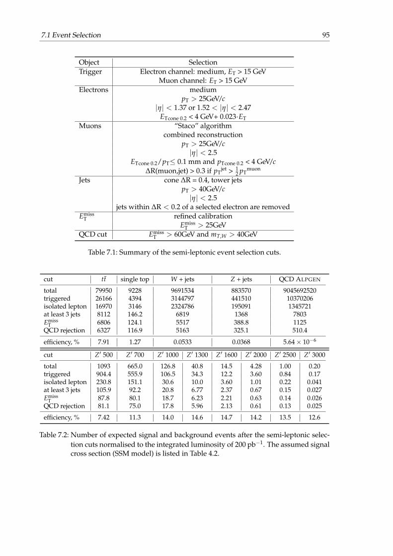
7.1 Event Selection 95
Object SelectionTrigger Electron channel: medium, ET > 15 GeV
Muon channel: ET > 15 GeVElectrons medium
pT > 25GeV/c|η| < 1.37 or 1.52 < |η| < 2.47
ETcone 0.2 < 4 GeV+ 0.023·ETMuons “Staco” algorithm
combined reconstructionpT > 25GeV/c|η| < 2.5
ETcone 0.2/pT≤ 0.1 mm and pTcone 0.2 < 4 GeV/c∆R(muon,jet) > 0.3 if pT
jet > 12 pT
muon
Jets cone ∆R = 0.4, tower jetspT > 40GeV/c|η| < 2.5
jets within ∆R < 0.2 of a selected electron are removedEmiss
T refined calibrationEmiss
T > 25GeVQCD cut Emiss
T > 60GeV and mT,W > 40GeV
Table 7.1: Summary of the semi-leptonic event selection cuts.
cut tt single top W + jets Z + jets QCD ALPGEN
total 79950 9228 9691534 883570 9045692520triggered 26166 4394 3144797 441510 10370206isolated lepton 16970 3146 2324786 195091 1345721at least 3 jets 8112 146.2 6819 1368 7803Emiss
T 6806 124.1 5517 388.8 1125QCD rejection 6327 116.9 5163 325.1 510.4
efficiency, % 7.91 1.27 0.0533 0.0368 5.64× 10⁻⁶
cut Z′ 500 Z′ 700 Z′ 1000 Z′ 1300 Z′ 1600 Z′ 2000 Z′ 2500 Z′ 3000
total 1093 665.0 126.8 40.8 14.5 4.28 1.00 0.20triggered 904.4 555.9 106.5 34.3 12.2 3.60 0.84 0.17isolated lepton 230.8 151.1 30.6 10.0 3.60 1.01 0.22 0.041at least 3 jets 105.9 92.2 20.8 6.77 2.37 0.67 0.15 0.027Emiss
T 87.8 80.1 18.7 6.23 2.21 0.63 0.14 0.026QCD rejection 81.1 75.0 17.8 5.96 2.13 0.61 0.13 0.025
efficiency, % 7.42 11.3 14.0 14.6 14.7 14.2 13.5 12.6
Table 7.2: Number of expected signal and background events after the semi-leptonic selec-tion cuts normalised to the integrated luminosity of 200 pb−1. The assumed signalcross section (SSM model) is listed in Table 4.2.

96 Chapter 7. The tt Invariant Mass Distribution
2
[GeV]TEraw
0 50 100
]2
) [G
eV
/cT
E(l
ep
,ra
w
Tm
0
50
100
150
= 10 TeVs
[GeV]TEraw
0 50 100
]2
) [G
eV
/cT
E(l
ep
,ra
w
Tm
0
50
100
1502m = 500 GeV/c
Z’
[GeV]TEraw
0 50 100
]2
) [G
eV
/cT
E(l
ep
,ra
w
Tm
0
50
100
150
= 10 TeVs
[GeV]TEraw
0 50 100
]2
) [G
eV
/cT
E(l
ep
,ra
w
Tm
0
50
100
150tt no had
[GeV]TEraw
0 50 100
]2
) [G
eV
/cT
E(l
ep
,ra
w
Tm
0
50
100
150
= 10 TeVs
[GeV]TEraw
0 50 100
]2
) [G
eV
/cT
E(l
ep
,ra
w
Tm
0
50
100
150tt full had
[GeV]TEraw
0 50 100
]2
) [G
eV
/cT
E(l
ep
,ra
w
Tm
0
50
100
150
= 10 TeVs
[GeV]TEraw
0 50 100
]2
) [G
eV
/cT
E(l
ep
,ra
w
Tm
0
50
100
150multijet
Figure 7.1: Missing transverse energy versus transverse W boson mass mT,W =mT(lep, rawEmiss
T ) for events with the high-pT leptons like in the semi-leptonicand di-leptonic tt events or fake leptons in the QCD multijet and in the tt fullyhadronic events. The Z′ boson sample contains all possible tt decay modes, alsofake leptons from the fully hadronic tt decays.
The number of expected events for signal and the main sources of background afterthe semi-leptonic selection cuts are listed in Table 7.2. They are given for the whole mtt-range and for an expected luminosity of 200 pb−1. The fraction of expected signal andbackground events under the Z′ boson mass peak, relevant for the sensitivity of the signalwill be discussed in Section 7.4. Now, we will discuss the overall selection efficiency for thesignal and background.
The signal selection efficiency is raising with increasing Z′ boson mass up to 14.7%. ForZ′ boson mass of 500 GeV/c2, the efficiency is comparable to the selection efficiency of ttbackground as expected. In the most interesting mass range between 1000 and 2000 GeV/c2
the signal selection efficiency is nearly constant and at its highest value for the chosen cuts.At Z′ boson masses larger than 2000 GeV/c2 the lepton isolation criterion leads to a decrease

7.1 Event Selection 97
Figure 7.2: Lepton trigger efficiency versus lepton pT for signal events after semi-leptonicselection cuts.
in the efficiency.
tt events have the highest contribution to the background, followed by W + jets events.About 7.9 % of all tt events are selected. The probability to select a W + jets event is of order0.05 %, but the production cross section is two magnitudes higher than for the tt events. TheQCD background is reduced by a factor 10−6. Z + jets events can pass the selection if oneof the leptons is not reconstructed and not selected. The selection probability is 0.037 %, butthe production cross section is a factor 10 lower compared to W + jets. The single top quarkbackground is the smallest one because of the small production rate and a low selectionefficiency. Additional jets are required to mimic the second top quark, therefore the selectionefficiency is lower than for the tt events.
To check the purity of the selected signal events, they have been categorised as di-leptonic, semi-leptonic and fully hadronic events using the Monte Carlo truth informa-tion. Tau leptons are counted as leptons only if taus decay leptonically, otherwise they arecounted as jets. The categories are:
• di-leptonic signature
ee, µµ + jets and eτ, µτ, ττ + jets with τ→ leptons (branching ratio ∼ 6.5%)
• semi-leptonic signature
I. e, µ + jets and τ + jets with τ→ leptons (branching ratio ∼ 34.6%)
II. eτ, µτ + jets with τ → hadrons and ττ + jets with one τ → leptons and one τ→ hadrons (branching ratio ∼ 3.5%)
• fully hadronic signature
jets and τ, ττ + jets with τ→ hadrons (branching ratio ∼ 55.3%)
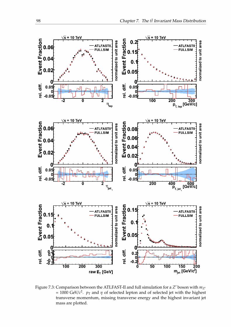
98 Chapter 7. The tt Invariant Mass Distribution
Figure 7.3: Comparison between the ATLFAST-II and full simulation for a Z′ boson with mZ′
= 1000 GeV/c2. pT and η of selected lepton and of selected jet with the highesttransverse momentum, missing transverse energy and the highest invariant jetmass are plotted.
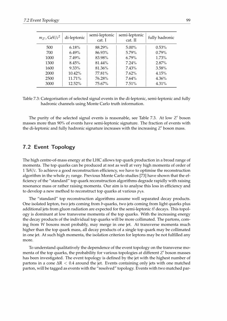
7.2 Event Topology 99
mZ′ , GeV/c2 di-leptonicsemi-leptonic semi-leptonic
fully hadroniccat. I cat. II
500 6.18% 88.29% 5.00% 0.53%700 6.49% 86.93% 5.79% 0.79%
1000 7.49% 83.98% 6.79% 1.73%1300 8.45% 81.44% 7.24% 2.87%1600 9.33% 81.36% 7.43% 3.58%2000 10.42% 77.81% 7.62% 4.15%2500 11.71% 76.28% 7.64% 4.36%3000 12.52% 75.67% 7.51% 4.31%
Table 7.3: Categorisation of selected signal events in the di-leptonic, semi-leptonic and fullyhadronic channels using Monte Carlo truth information.
The purity of the selected signal events is reasonable, see Table 7.3. At low Z′ bosonmasses more than 90% of events have semi-leptonic signature. The fraction of events withthe di-leptonic and fully hadronic signature increases with the increasing Z′ boson mass.
7.2 Event Topology
The high centre-of-mass energy at the LHC allows top quark production in a broad range ofmomenta. The top quarks can be produced at rest as well at very high momenta of order of1 TeV/c. To achieve a good reconstruction efficiency, we have to optimise the reconstructionalgorithm in the whole pT range. Previous Monte Carlo studies [73] have shown that the ef-ficiency of the “standard” top quark reconstruction algorithms degrade rapidly with raisingresonance mass or rather raising momenta. Our aim is to analyse this loss in efficiency andto develop a new method to reconstruct top quarks at various pTs.
The “standard” top reconstruction algorithms assume well separated decay products.One isolated lepton, two jets coming from b-quarks, two jets coming from light quarks plusadditional jets from gluon radiation are expected for the semi-leptonic tt decays. This topol-ogy is dominant at low transverse momenta of the top quarks. With the increasing energythe decay products of the individual top quarks will be more collimated. The partons, com-ing from W bosons most probably, may merge in one jet. At transverse momenta muchhigher than the top quark mass, all decay products of a single top quark may be collimatedin one jet. At such high momenta, the isolation criterion for leptons may be not fulfilled anymore.
To understand qualitatively the dependence of the event topology on the transverse mo-menta of the top quarks, the probability for various topologies at different Z′ boson masseshas been investigated. The event topology is defined by the jet with the highest number ofpartons in a cone ∆R < 0.4 around the jet. Events containing only jets with one matchedparton, will be tagged as events with the “resolved” topology. Events with two matched par-
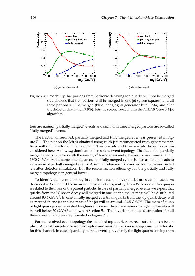
100 Chapter 7. The tt Invariant Mass Distribution
(a) generator level (b) detector level
Figure 7.4: Probability that partons from hadronic decaying top quarks will not be merged(red circles), that two partons will be merged in one jet (green squares) and allthree partons will be merged (blue triangles) at generator level 7.5(a) and afterthe detector simulation 7.5(b). Jets are reconstructed with the ATLAS Cone 0.4 jetalgorithm.
tons are named “partially merged” events and such with three merged partons are so-called“fully merged” events.
The fraction of resolved, partially merged and fully merged events is presented in Fig-ure 7.4. The plot on the left is obtained using truth jets reconstructed from generator par-ticles without detector simulation. Only tt → e + jets and tt → µ + jets decay modes areconsidered here. At low mtt dominates the resolved event topology. The fraction of partiallymerged events increases with the raising Z′ boson mass and achieves its maximum at about1600 GeV/c2. At the same time the amount of fully merged events is increasing and leads toa decrease of partially merged events. A similar behaviour is observed for the reconstructedjets after detector simulation. But the reconstruction efficiency for the partially and fullymerged topology is in general lower.
To identify the event topology in collision data, the invariant jet mass can be used. Asdiscussed in Section 5.4 the invariant mass of jets originating from W bosons or top quarksis related to the mass of the parent particle. In case of partially merged events we expect thatquarks from the W boson decay will merged in one jet and the jet mass will be distributedaround 80.4 GeV/c2. In case of fully merged events, all quarks from the top quark decay willbe merged in one jet and the mass of the jet will be around 172.5 GeV/c2. The mass of gluonor light quark jets is generated by gluon emission. Thus, the masses of single parton jets willbe well below 50 GeV/c2 as shown in Section 5.4. The invariant jet mass distributions for allthree event topologies are presented in Figure 7.5.
For the resolved event topology the standard top quark pairs reconstruction can be ap-plied. At least four jets, one isolated lepton and missing transverse energy are characteristicfor this channel. In case of partially merged events prevalently the light quarks coming from
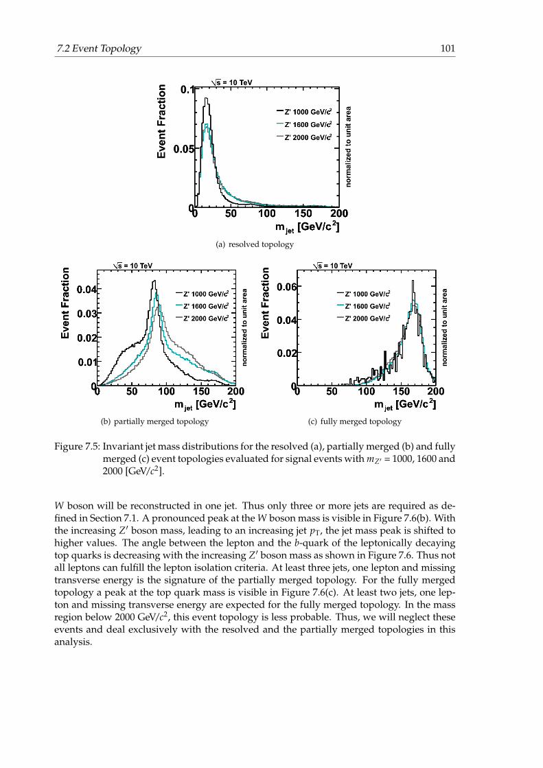
7.2 Event Topology 101
(a) resolved topology
(b) partially merged topology (c) fully merged topology
Figure 7.5: Invariant jet mass distributions for the resolved (a), partially merged (b) and fullymerged (c) event topologies evaluated for signal events with mZ′ = 1000, 1600 and2000 [GeV/c2].
W boson will be reconstructed in one jet. Thus only three or more jets are required as de-fined in Section 7.1. A pronounced peak at the W boson mass is visible in Figure 7.6(b). Withthe increasing Z′ boson mass, leading to an increasing jet pT, the jet mass peak is shifted tohigher values. The angle between the lepton and the b-quark of the leptonically decayingtop quarks is decreasing with the increasing Z′ boson mass as shown in Figure 7.6. Thus notall leptons can fulfill the lepton isolation criteria. At least three jets, one lepton and missingtransverse energy is the signature of the partially merged topology. For the fully mergedtopology a peak at the top quark mass is visible in Figure 7.6(c). At least two jets, one lep-ton and missing transverse energy are expected for the fully merged topology. In the massregion below 2000 GeV/c2, this event topology is less probable. Thus, we will neglect theseevents and deal exclusively with the resolved and the partially merged topologies in thisanalysis.

102 Chapter 7. The tt Invariant Mass Distribution
(a) resolved topology
(b) partially merged topology (c) fully merged topology
Figure 7.6: The angle between the true lepton and the b-quark ∆R(mc_lep,bquark) for theresolved (a), partially merged (b) and fully merged (c) event topologies evaluatedfor signal events with mZ′ = 1000, 1600 and 2000 [GeV/c2].
7.3 Analysis Strategy
This reconstruction approach is designed for the tt resonance searches in the early stage ofthe experiment. The strategy is to keep the signal efficiency as high as possible and to useas less observables as possible. The goal is to reduce the systematic uncertainty and to testa wide range of mtt also increasing the sensitivity in a mass range which is currently testedby DØ and CDF.
No attempt is made to fully reconstruct the individual top quarks to calculate mtt. Theinvariant mass is reconstructed by summing up the four momenta of the selected jets, thelepton and the reconstructed neutrino. The number of required jets depends on the eventtopology, which is defined using the highest invariant jet mass in the event. The events are

7.3 Analysis Strategy 103
(a) number jets (b) highest jet mass
Figure 7.7: Number of reconstructed jets (a) and the highest invariant jet mass in the 3 jet bin(b) after selection cuts for the main background processes and a signal processwith mZ′=1000 GeV/c2.
separated into sub-samples with different jet multiplicities and jet masses. That allows toprepare a topology-dependent reconstruction of signal events. The composition and the sizeof background varies for different sub-samples. The events can be separated in a very signalpure and in a background enriched sub-samples to optimise the sensitivity for the signal ina wide mtt range.
The selected events are classified in the following way:
• 4 jets sub-sample
events containing four jets are suppose to be fully resolved events. The four jets,the lepton and reconstructed neutrino are used to compute the tt invariant mass.
• 5 or more jets sub-sample
events containing more than four jets are supposed to be fully resolved eventswith additional jets from gluon radiation. The four jets with highest transversemomenta, the lepton and reconstructed neutrino are used to compute the tt in-variant mass.
• 3 jets low and high jet mass sub-samples
events containing three jets are supposed to have merged jets. These events aresplit into two sub-samples according to the highest jet mass mjet found in theevent. The cut value is chosen in the way to separate events in a backgrounddominated and a signal dominated regions. The first sub-sample consist of threejet events with mjet below 65 GeV/c2, three jet events with mjet above 65 GeV/c2
forming the second sub-sample. The three jets, the lepton and reconstructed neu-trino are used to compute the tt invariant mass.
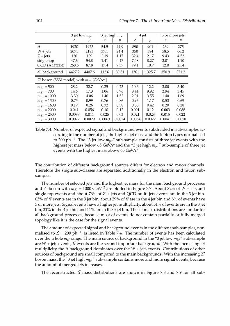
104 Chapter 7. The tt Invariant Mass Distribution
3 jet low mjet 3 jet high mjet 4 jet 5 or more jetse µ e µ e µ e µ
tt 1920 1973 54.5 44.9 890 901 269 275W + jets 2071 2183 37.1 24.4 350 384 58.5 66.2Z + jets 120 109 2.19 1.17 32.4 21.7 9.43 4.52single top 47.6 54.8 1.41 0.47 7.48 8.27 2.01 1.10QCD (ALPGEN) 268.6 87.8 17.4 9.37 79.1 10.7 12.0 25.4
all background 4427.2 4407.6 112.6 80.31 1361 1325.7 350.9 371.2
Z′ boson (SSM model) with mZ′ [GeV/c2]
mZ′ = 500 28.2 32.7 0.25 0.23 10.6 12.2 3.00 3.40mZ′ = 700 14.6 17.3 1.06 0.96 8.44 9.92 2.94 3.45mZ′ = 1000 3.30 4.06 1.46 1.52 2.91 3.55 1.40 1.69mZ′ = 1300 0.75 0.99 0.76 0.86 0.93 1.17 0.53 0.69mZ′ = 1600 0.19 0.26 0.32 0.38 0.33 0.42 0.20 0.28mZ′ = 2000 0.041 0.056 0.10 0.12 0.091 0.12 0.063 0.088mZ′ = 2500 0.0083 0.011 0.025 0.03 0.021 0.028 0.015 0.022mZ′ = 3000 0.0022 0.0029 0.0063 0.0074 0.0054 0.0072 0.0041 0.0058
Table 7.4: Number of expected signal and background events subdivided in sub-samples ac-cording to the number of jets, the highest jet mass and the lepton types normalisedto 200 pb−1. The “3 jet low mjet” sub-sample consists of three jet events with thehighest jet mass below 65 GeV/c2and the “3 jet high mjet” sub-sample of three jetevents with the highest mass above 65 GeV/c2.
The contribution of different background sources differs for electron and muon channels.Therefore the single sub-classes are separated additionally in the electron and muon sub-samples.
The number of selected jets and the highest jet mass for the main background processesand Z′ boson with mZ′ = 1000 GeV/c2 are plotted in Figure 7.7. About 82% of W + jets andsingle top events and about 76% of Z + jets and QCD multi-jets events are in the 3 jet bin.63% of tt events are in the 3 jet bin, about 29% of tt are in the 4 jet bin and 8% of events have5 or more jets. Signal events have a higher jet multiplicity, about 51% of events are in the 3 jetbin, 31% in the 4 jet bin and 11% are in the 5 jet bin. The jet mass distributions are similar forall background processes, because most of events do not contain partially or fully mergedtopology like it is the case for the signal events.
The amount of expected signal and background events in the different sub-samples, nor-malised to L = 200 pb−1, is listed in Table 7.4. The number of events has been calculatedover the whole mtt range. The main source of background in the “3 jet low mjet” sub-sampleare W + jets events, tt events are the second important background. With the increasing jetmultiplicity the tt background dominates over the W + jets events. Contributions of othersources of background are small compared to the main backgrounds. With the increasing Z′
boson mass, the “3 jet high mjet” sub-sample contains more and more signal events, becausethe amount of merged jets increases.
The reconstructed tt mass distributions are shown in Figure 7.8 and 7.9 for all sub-

7.4 Selection Efficiency and Mass Resolution 105
(a) electron + 3 jets, low mjet (b) muon + 3 jets, low mjet
(c) electron + 3 jets, high mjet (d) muon + 3 jets, high mjet
Figure 7.8: The tt invariant mass distributions in 3 jet channel for electron + 3 jets, low mjet(a), muon + 3 jets, low mjet (b), electron + 3 jets, high mjet (c) and muon + 3 jets,high mjet (d) sub-samples. The Z′ boson cross section (SSM model) has beenmultiplied by a factor of 50.
samples. The signal events are scaled by a factor of 50 for a better visibility. Not only theamount of events, but also the mtt shape differs for individual sub-samples for the signaland as well as for the background.
7.4 Selection Efficiency and Mass Resolution
In this section we will give an estimate for the sensitivity of this analysis for tt resonancesin different sub-samples. We will focus on two aspects: the event selection efficiency in amass window around the reconstructed resonance peak and the mass resolution. The ratio
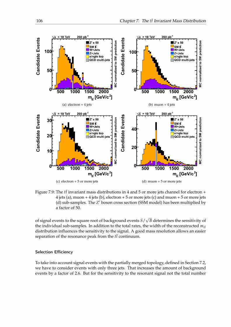
106 Chapter 7. The tt Invariant Mass Distribution
(a) electron + 4 jets (b) muon + 4 jets
(c) electron + 5 or more jets (d) muon + 5 or more jets
Figure 7.9: The tt invariant mass distributions in 4 and 5 or more jets channel for electron +4 jets (a), muon + 4 jets (b), electron + 5 or more jets (c) and muon + 5 or more jets(d) sub-samples. The Z′ boson cross section (SSM model) has been multiplied bya factor of 50.
of signal events to the square root of background events S/√
B determines the sensitivity ofthe individual sub-samples. In addition to the total rates, the width of the reconstructed mttdistribution influences the sensitivity to the signal. A good mass resolution allows an easierseparation of the resonance peak from the tt continuum.
Selection Efficiency
To take into account signal events with the partially merged topology, defined in Section 7.2,we have to consider events with only three jets. That increases the amount of backgroundevents by a factor of 2.6. But for the sensitivity to the resonant signal not the total number
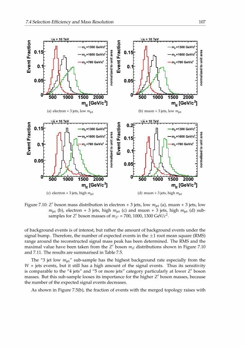
7.4 Selection Efficiency and Mass Resolution 107
(a) electron + 3 jets, low mjet (b) muon + 3 jets, low mjet
(c) electron + 3 jets, high mjet (d) muon + 3 jets, high mjet
Figure 7.10: Z′ boson mass distribution in electron + 3 jets, low mjet (a), muon + 3 jets, lowmjet (b), electron + 3 jets, high mjet (c) and muon + 3 jets, high mjet (d) sub-samples for Z′ boson masses of mZ′ = 700, 1000, 1300 GeV/c2.
of background events is of interest, but rather the amount of background events under thesignal bump. Therefore, the number of expected events in the ±1 root mean square (RMS)range around the reconstructed signal mass peak has been determined. The RMS and themaximal value have been taken from the Z′ boson mtt distributions shown in Figure 7.10and 7.11. The results are summarised in Table 7.5.
The “3 jet low mjet” sub-sample has the highest background rate especially from theW + jets events, but it still has a high amount of the signal events. Thus its sensitivityis comparable to the “4 jets” and “5 or more jets” category particularly at lower Z′ bosonmasses. But this sub-sample looses its importance for the higher Z′ boson masses, becausethe number of the expected signal events decreases.
As shown in Figure 7.5(b), the fraction of events with the merged topology raises with

108 Chapter 7. The tt Invariant Mass Distribution
(a) electron + 4 jets (b) muon + 4 jets
(c) electron + 5 or more jets (d) muon + 5 or more jets
Figure 7.11: Z′ boson mass distribution in electron + 4 jets (a), muon + 4 jets (b), electron + 5or more jets (c) and muon + 5 or more jets (d) sub-samples for Z′ boson massesof mZ′ = 700, 1000, 1300 GeV/c2.
the increasing Z′ boson mass. More and more signal events populate the “3 jet high mjet”category. Due to a low background rate in this category, it has the best S/
√B ratio especially
at high Z′ boson masses.
The S/√
B ratio of the “4 jet” and “5 or more jets” sub-samples is of the same size. Themuon channel is slightly more sensitive for all event topologies, because a higher signal se-lection efficiency prevails a partly higher background selection efficiency. Finally the combi-nation of all sub-samples provides the sensitivity in a broad mass range from twice the topquark mass into the TeV-regime.
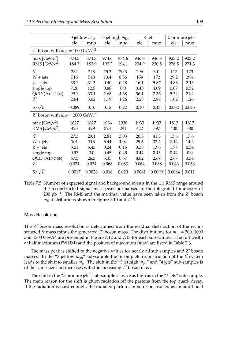
7.4 Selection Efficiency and Mass Resolution 109
3 jet low mjet 3 jet high mjet 4 jet 5 or more jetsele muo ele muo ele muo ele muo
Z′ boson with mZ′ = 1000 GeV/c2
max [GeV/c2] 874.3 874.3 974.6 974.6 946.3 946.3 923.2 923.2RMS [GeV/c2] 184.3 183.9 193.2 194.1 234.9 230.5 276.5 271.3
tt 232 243 25.2 20.3 296 301 117 123W + jets 516 548 13.4 8.36 159 172 29.2 29.4Z + jets 33.1 31.3 0.40 0.48 16.1 9.87 4.83 2.15single top 7.26 12.8 0.88 0.0 3.45 4.09 0.07 0.52QCD (ALPGEN) 99.1 33.4 2.68 4.68 36.1 7.36 5.34 21.4Z′ 2.64 3.02 1.19 1.26 2.28 2.84 1.02 1.26
S/√
B 0.089 0.10 0.18 0.22 0.10 0.13 0.082 0.095
Z′ boson with mZ′ = 2000 GeV/c2
max [GeV/c2] 1627 1627 1936 1936 1933 1933 1813 1813RMS [GeV/c2] 423 429 328 291 422 397 400 380
tt 27.3 29.1 2.81 3.03 20.3 41.3 13.6 17.6W + jets 101 115 5.44 4.04 29.6 32.4 7.44 14.4Z + jets 8.01 6.43 0.24 0.16 3.38 1.96 1.77 0.54single top 0.97 0.0 0.45 0.45 0.44 0.45 0.44 0.0QCD (ALPGEN) 67.5 26.3 5.35 0.67 8.02 2.67 2.67 3.34Z′ 0.024 0.034 0.068 0.083 0.064 0.088 0.043 0.063
S/√
B 0.0017 0.0026 0.018 0.029 0.0081 0.0099 0.0084 0.011
Table 7.5: Number of expected signal and background events in the ±1 RMS range aroundthe reconstructed signal mass peak normalised to the integrated luminosity of200 pb−1. The RMS and the maximal value have been taken from the Z′ bosonmtt distributions shown in Figure 7.10 and 7.11.
Mass Resolution
The Z′ boson mass resolution is determined from the residual distribution of the recon-structed tt mass minus the generated Z′ boson mass. The distributions for mZ′ = 700, 1000and 1300 GeV/c2 are presented in Figure 7.12 and 7.13 for each sub-sample. The full widthat half maximum (FWHM) and the position of maximum (max) are listed in Table 7.6.
The mass peak is shifted to the negative values for nearly all sub-samples and Z′ bosonmasses. In the “3 jet low mjet” sub-sample the incomplete reconstruction of the tt systemleads to the shift to smaller mtt. The shift in the “3 jet high mjet” and “4 jets” sub-samples isof the same size and increases with the increasing Z′ boson mass.
The shift in the “5 or more jets” sub-sample is twice as high as in the “4 jets” sub-sample.The main reason for the shift is gluon radiation off the partons from the top quark decay.If the radiation is hard enough, the radiated parton can be reconstructed as an additional
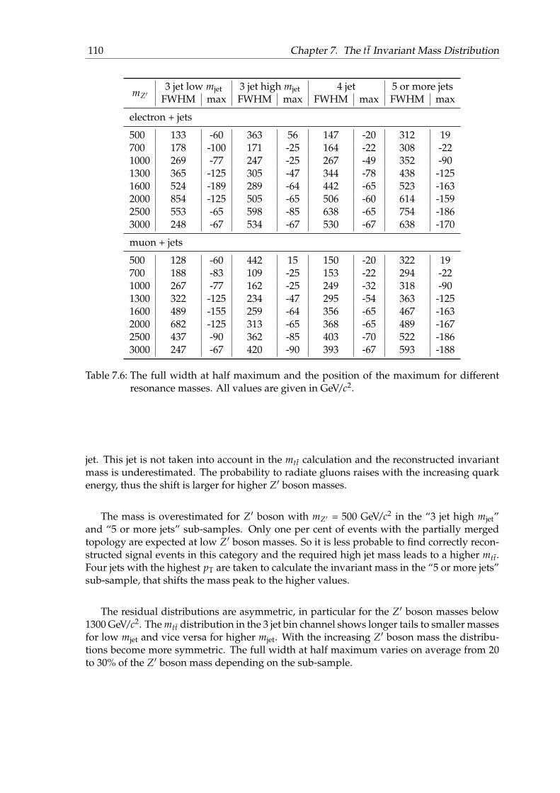
110 Chapter 7. The tt Invariant Mass Distribution
mZ′3 jet low mjet 3 jet high mjet 4 jet 5 or more jets
FWHM max FWHM max FWHM max FWHM max
electron + jets
500 133 -60 363 56 147 -20 312 19700 178 -100 171 -25 164 -22 308 -221000 269 -77 247 -25 267 -49 352 -901300 365 -125 305 -47 344 -78 438 -1251600 524 -189 289 -64 442 -65 523 -1632000 854 -125 505 -65 506 -60 614 -1592500 553 -65 598 -85 638 -65 754 -1863000 248 -67 534 -67 530 -67 638 -170
muon + jets
500 128 -60 442 15 150 -20 322 19700 188 -83 109 -25 153 -22 294 -221000 267 -77 162 -25 249 -32 318 -901300 322 -125 234 -47 295 -54 363 -1251600 489 -155 259 -64 356 -65 467 -1632000 682 -125 313 -65 368 -65 489 -1672500 437 -90 362 -85 403 -70 522 -1863000 247 -67 420 -90 393 -67 593 -188
Table 7.6: The full width at half maximum and the position of the maximum for differentresonance masses. All values are given in GeV/c2.
jet. This jet is not taken into account in the mtt calculation and the reconstructed invariantmass is underestimated. The probability to radiate gluons raises with the increasing quarkenergy, thus the shift is larger for higher Z′ boson masses.
The mass is overestimated for Z′ boson with mZ′ = 500 GeV/c2 in the “3 jet high mjet”and “5 or more jets” sub-samples. Only one per cent of events with the partially mergedtopology are expected at low Z′ boson masses. So it is less probable to find correctly recon-structed signal events in this category and the required high jet mass leads to a higher mtt.Four jets with the highest pT are taken to calculate the invariant mass in the “5 or more jets”sub-sample, that shifts the mass peak to the higher values.
The residual distributions are asymmetric, in particular for the Z′ boson masses below1300 GeV/c2. The mtt distribution in the 3 jet bin channel shows longer tails to smaller massesfor low mjet and vice versa for higher mjet. With the increasing Z′ boson mass the distribu-tions become more symmetric. The full width at half maximum varies on average from 20to 30% of the Z′ boson mass depending on the sub-sample.
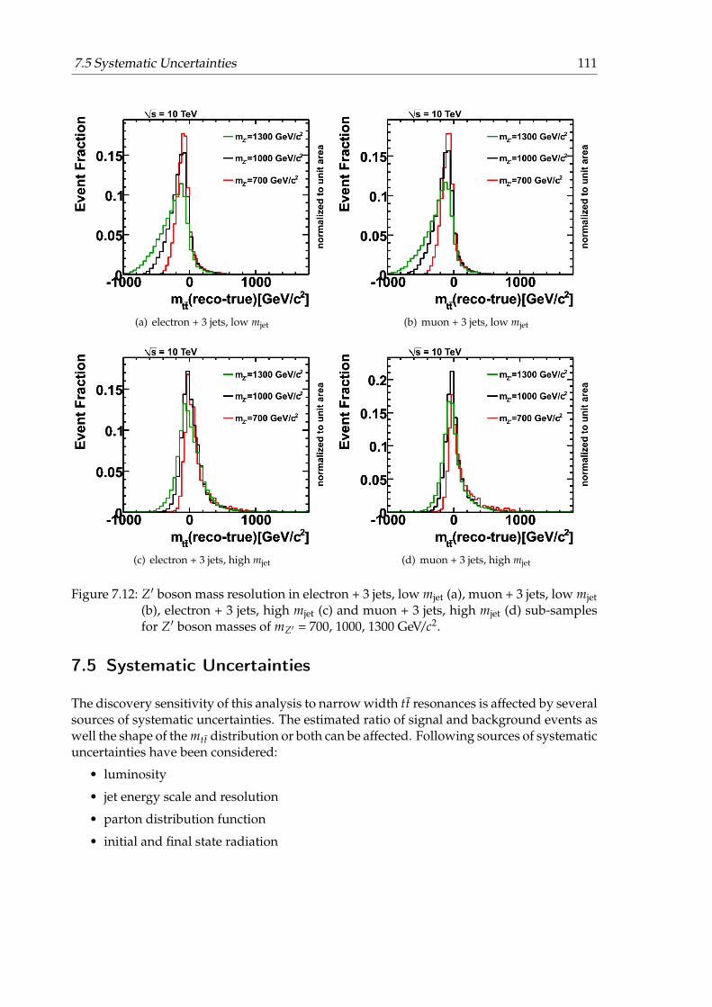
7.5 Systematic Uncertainties 111
(a) electron + 3 jets, low mjet (b) muon + 3 jets, low mjet
(c) electron + 3 jets, high mjet (d) muon + 3 jets, high mjet
Figure 7.12: Z′ boson mass resolution in electron + 3 jets, low mjet (a), muon + 3 jets, low mjet(b), electron + 3 jets, high mjet (c) and muon + 3 jets, high mjet (d) sub-samplesfor Z′ boson masses of mZ′ = 700, 1000, 1300 GeV/c2.
7.5 Systematic Uncertainties
The discovery sensitivity of this analysis to narrow width tt resonances is affected by severalsources of systematic uncertainties. The estimated ratio of signal and background events aswell the shape of the mtt distribution or both can be affected. Following sources of systematicuncertainties have been considered:
• luminosity
• jet energy scale and resolution
• parton distribution function
• initial and final state radiation
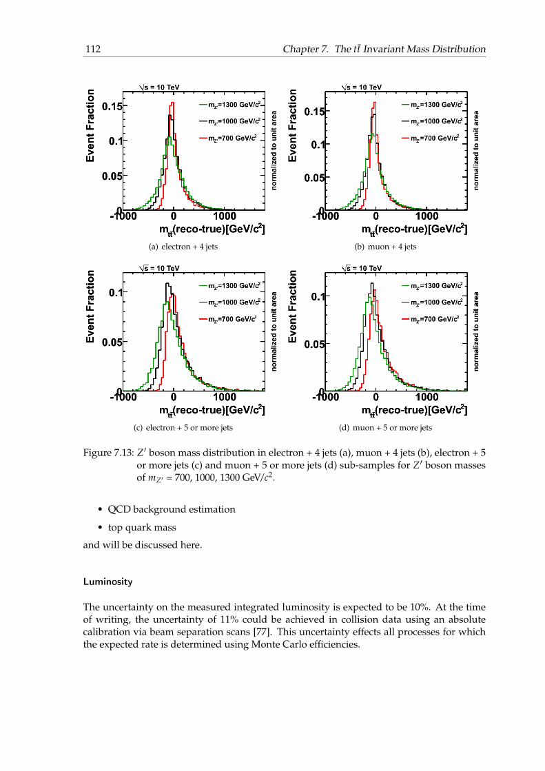
112 Chapter 7. The tt Invariant Mass Distribution
(a) electron + 4 jets (b) muon + 4 jets
(c) electron + 5 or more jets (d) muon + 5 or more jets
Figure 7.13: Z′ boson mass distribution in electron + 4 jets (a), muon + 4 jets (b), electron + 5or more jets (c) and muon + 5 or more jets (d) sub-samples for Z′ boson massesof mZ′ = 700, 1000, 1300 GeV/c2.
• QCD background estimation
• top quark mass
and will be discussed here.
Luminosity
The uncertainty on the measured integrated luminosity is expected to be 10%. At the timeof writing, the uncertainty of 11% could be achieved in collision data using an absolutecalibration via beam separation scans [77]. This uncertainty effects all processes for whichthe expected rate is determined using Monte Carlo efficiencies.
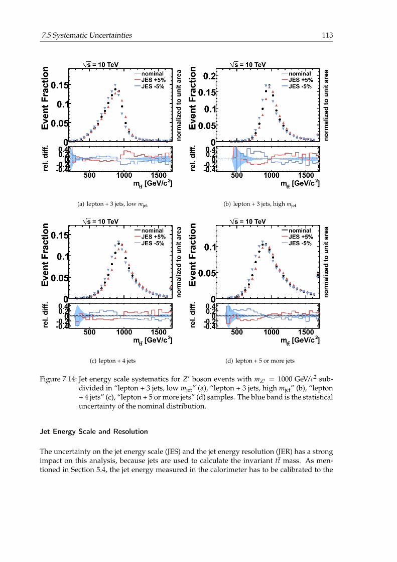
7.5 Systematic Uncertainties 113
(a) lepton + 3 jets, low mjet (b) lepton + 3 jets, high mjet
(c) lepton + 4 jets (d) lepton + 5 or more jets
Figure 7.14: Jet energy scale systematics for Z′ boson events with mZ′ = 1000 GeV/c2 sub-divided in “lepton + 3 jets, low mjet” (a), “lepton + 3 jets, high mjet” (b), “lepton+ 4 jets” (c), “lepton + 5 or more jets” (d) samples. The blue band is the statisticaluncertainty of the nominal distribution.
Jet Energy Scale and Resolution
The uncertainty on the jet energy scale (JES) and the jet energy resolution (JER) has a strongimpact on this analysis, because jets are used to calculate the invariant tt mass. As men-tioned in Section 5.4, the jet energy measured in the calorimeter has to be calibrated to the

114 Chapter 7. The tt Invariant Mass Distribution
(a) lepton + 3 jets, low mjet (b) lepton + 3 jets, high mjet
(c) lepton + 4 jets (d) lepton + 5 or more jets
Figure 7.15: Jet energy scale systematics for tt events sub-divided in “lepton + 3 jets, lowmjet” (a), “lepton + 3 jets, high mjet” (b), “lepton + 4 jets” (c), “lepton + 5 or morejets” (d) samples. The blue band is the statistical uncertainty of the nominaldistribution.
hadronic energy scale using a detailed simulation of hadronic showers in the detector. Thiscalibration can systematically shift the jet energy to higher or lower values. Additionallythe jet energy resolution could be underestimated in the Monte Carlo simulations comparedto the measured resolution in collision data. Both affect the sensitivity to the signal. To es-timate the impact of these uncertainties on the analysis, the energy of all selected jets have

7.5 Systematic Uncertainties 115
(a) lepton + 3 jets, low mjet (b) lepton + 3 jets, high mjet
(c) lepton + 4 jets (d) lepton + 5 or more jets
Figure 7.16: Jet energy resolution systematics for Z′ boson events with mZ′ = 1000 GeV/c2
sub-divided in “lepton + 3 jets, low mjet” (a), “lepton + 3 jets, high mjet” (b),“lepton + 4 jets” (c), “lepton + 5 or more jets” (d) samples. The blue band is thestatistical uncertainty of the nominal distribution.
been scaled up and down by 5% and have been smeared by a Gaussian function with thewidth of 25%√
Ejet+ 5%. For each jet a random number is generated from this Gaussian function
and the jet energy is scaled by this number. Missing transverse energy is calculated from thetotal energy balance of the event. Thus, the difference between the unscaled and scaled jetenergy is vectorially added to Emiss
T .

116 Chapter 7. The tt Invariant Mass Distribution
The influence of the jet energy scale variation on the reconstructed mtt shape for the sig-nal events can be seen in Figure 7.14 and for the tt background events in Figure 7.15. Theelectron and muon channels are combined in the plots, because this systematic uncertaintyaffects the mtt shapes of both channels in the same way. The shift of the jet energy scale leadsto the shift of the Z′ boson mass peak, the relative difference of the nominal and shifted dis-tributions is of order 20-25%. The background shapes are not affected, the relative differenceof the nominal and shifted distributions is of the same order as the statistical uncertainty.
Figure 7.16 presents the jet energy resolution uncertainty for the signal events. An ad-ditional smearing of the jet energy has a small effect on the mtt distributions. The maximalrelative difference between the nominal and smeared distributions is about 10%.
Not only the shapes, but also the number of expected signal and background events areaffected. The relative uncertainty on the number of events is listed in Table 7.7. The negativeshift of JES leads to an overall loss of events or to a migration of events to the lower jet binsand for the positive shift vice versa. The jet energy smearing leads to an increase of thebackground and a decrease of signal events in the 3 jet bin.
Parton Distribution Function
The systematic uncertainty due to the choice of the parametrisation of the parton distribu-tion functions (PDF) used for the signal event simulation is examined by a re-weightingscheme. It uses Monte Carlo truth information about the hard partons that participated inthe hard process. The probability of an event with a particular kinematic characteristic tobe produced is evaluated and re-weighted according to the new values of the PDFs. TheCTEQ6LL [29] is default PDF set used to simulate signal events and the MRST2001LO [127]as an alternative PDF set.
Reconstructed mtt distribution for signal events is shown in Figure 7.17. The shapes ofdistributions in the peak region are not affected at all. The relative change in the number ofexpected signal events can be found in Table 7.7 and is around 3%.
Initial and Final State Radiation
To estimate the uncertainty due to the modeling of initial (ISR) and final (FSR) state radiationfor signal events, two samples have been produced for which the simulation is altered toproduce either less or more gluon radiation compared to the nominal settings. The ΛQCDvalue in the strong coupling αS controlling the parton shower has been varied to enhancethe initial state radiation and at the same tome to suppress the final state radiation and viceversa.
Figure 7.18 presents the mtt shapes of the nominal and altered distributions. The relativechange is of order of 5-10%, in the tails prevails the statistical uncertainty. The suppressedfinal state radiation results in a higher energy jets, which can more easily pass the selectioncuts and the number of selected events raises in the higher jet bins as shown in Table 7.7.
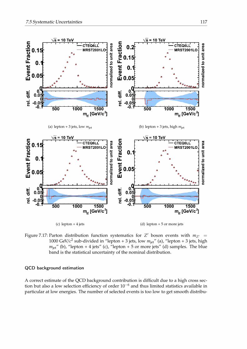
7.5 Systematic Uncertainties 117
(a) lepton + 3 jets, low mjet (b) lepton + 3 jets, high mjet
(c) lepton + 4 jets (d) lepton + 5 or more jets
Figure 7.17: Parton distribution function systematics for Z′ boson events with mZ′ =1000 GeV/c2 sub-divided in “lepton + 3 jets, low mjet” (a), “lepton + 3 jets, highmjet” (b), “lepton + 4 jets” (c), “lepton + 5 or more jets” (d) samples. The blueband is the statistical uncertainty of the nominal distribution.
QCD background estimation
A correct estimate of the QCD background contribution is difficult due to a high cross sec-tion but also a low selection efficiency of order 10−6 and thus limited statistics available inparticular at low energies. The number of selected events is too low to get smooth distribu-
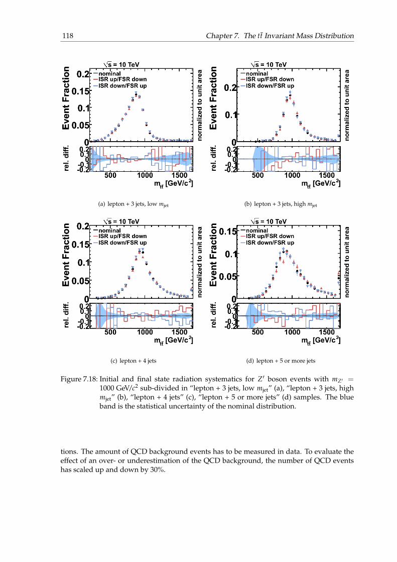
118 Chapter 7. The tt Invariant Mass Distribution
(a) lepton + 3 jets, low mjet (b) lepton + 3 jets, high mjet
(c) lepton + 4 jets (d) lepton + 5 or more jets
Figure 7.18: Initial and final state radiation systematics for Z′ boson events with mZ′ =1000 GeV/c2 sub-divided in “lepton + 3 jets, low mjet” (a), “lepton + 3 jets, highmjet” (b), “lepton + 4 jets” (c), “lepton + 5 or more jets” (d) samples. The blueband is the statistical uncertainty of the nominal distribution.
tions. The amount of QCD background events has to be measured in data. To evaluate theeffect of an over- or underestimation of the QCD background, the number of QCD eventshas scaled up and down by 30%.

7.5 Systematic Uncertainties 119
Figure 7.19: The reconstructed tt mass distribution for tt sample with different top quarkmasses. The events are sub-divided in “lepton + 3 jets, low mjet” (a), “lepton + 3jets, high mjet” (b), “lepton + 4 jets” (c), “lepton + 5 or more jets” (d) samples. Theblue band is the statistical uncertainty of the mtop = 172.5 GeV/c2 distribution.
Top Quark Mass
The mass of the top quark influences the kinematic properties of its decay products. Thus, itcan affect the shape of the mtt distribution. Figure 7.19 demonstrates that the changes due tothe top quark mass uncertainty are negligible. The uncertainty on the top quark mass willhave also a small effect on the mtt distribution of the signal events, because the resonancemass is much larger than 2·mtop.
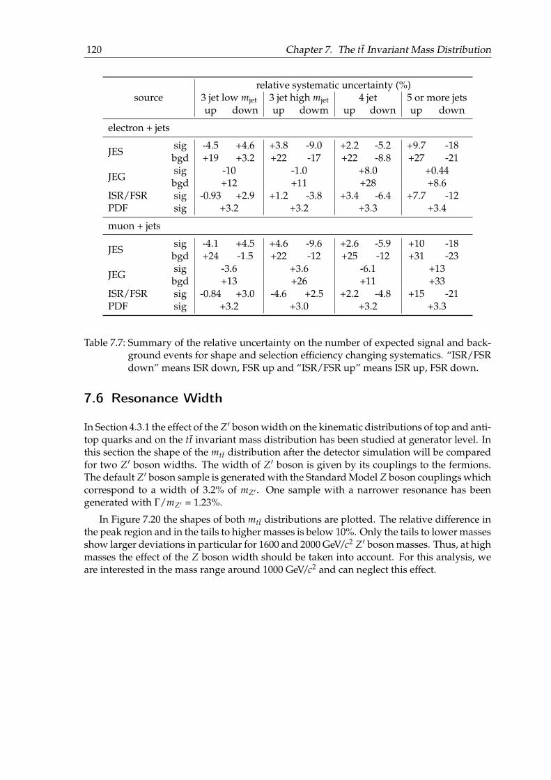
120 Chapter 7. The tt Invariant Mass Distribution
relative systematic uncertainty (%)source 3 jet low mjet 3 jet high mjet 4 jet 5 or more jets
up down up dowm up down up down
electron + jets
JESsig -4.5 +4.6 +3.8 -9.0 +2.2 -5.2 +9.7 -18bgd +19 +3.2 +22 -17 +22 -8.8 +27 -21
JEGsig -10 -1.0 +8.0 +0.44bgd +12 +11 +28 +8.6
ISR/FSR sig -0.93 +2.9 +1.2 -3.8 +3.4 -6.4 +7.7 -12PDF sig +3.2 +3.2 +3.3 +3.4
muon + jets
JESsig -4.1 +4.5 +4.6 -9.6 +2.6 -5.9 +10 -18bgd +24 -1.5 +22 -12 +25 -12 +31 -23
JEGsig -3.6 +3.6 -6.1 +13bgd +13 +26 +11 +33
ISR/FSR sig -0.84 +3.0 -4.6 +2.5 +2.2 -4.8 +15 -21PDF sig +3.2 +3.0 +3.2 +3.3
Table 7.7: Summary of the relative uncertainty on the number of expected signal and back-ground events for shape and selection efficiency changing systematics. “ISR/FSRdown” means ISR down, FSR up and “ISR/FSR up” means ISR up, FSR down.
7.6 Resonance Width
In Section 4.3.1 the effect of the Z′ boson width on the kinematic distributions of top and anti-top quarks and on the tt invariant mass distribution has been studied at generator level. Inthis section the shape of the mtt distribution after the detector simulation will be comparedfor two Z′ boson widths. The width of Z′ boson is given by its couplings to the fermions.The default Z′ boson sample is generated with the Standard Model Z boson couplings whichcorrespond to a width of 3.2% of mZ′ . One sample with a narrower resonance has beengenerated with Γ/mZ′ = 1.23%.
In Figure 7.20 the shapes of both mtt distributions are plotted. The relative difference inthe peak region and in the tails to higher masses is below 10%. Only the tails to lower massesshow larger deviations in particular for 1600 and 2000 GeV/c2 Z′ boson masses. Thus, at highmasses the effect of the Z boson width should be taken into account. For this analysis, weare interested in the mass range around 1000 GeV/c2 and can neglect this effect.
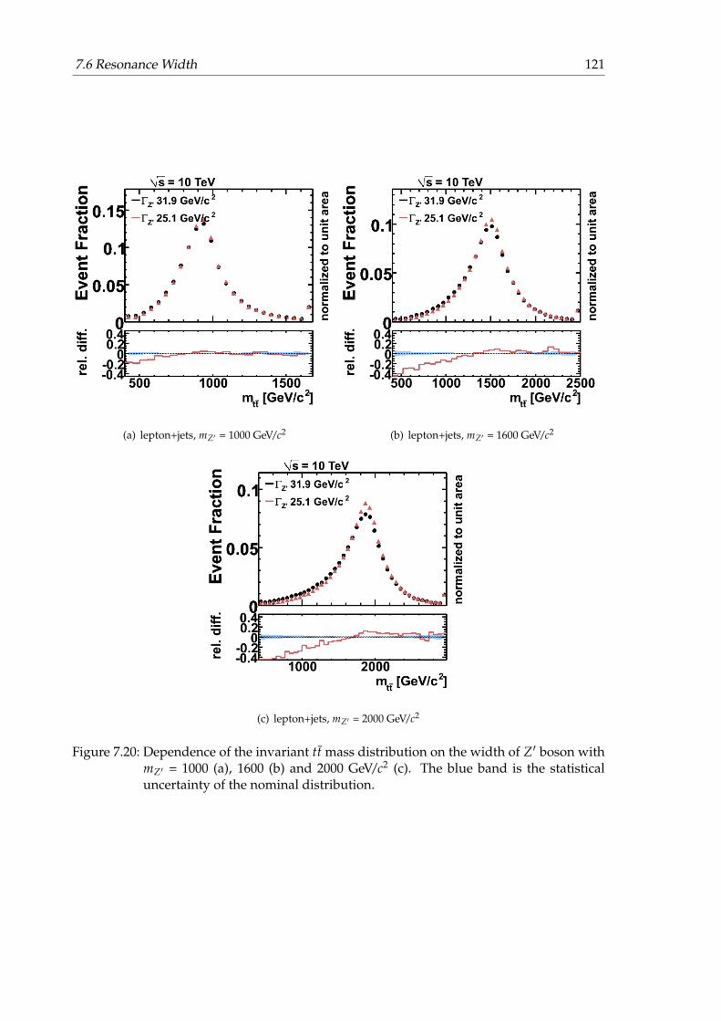
7.6 Resonance Width 121
(a) lepton+jets, mZ′ = 1000 GeV/c2 (b) lepton+jets, mZ′ = 1600 GeV/c2
(c) lepton+jets, mZ′ = 2000 GeV/c2
Figure 7.20: Dependence of the invariant tt mass distribution on the width of Z′ boson withmZ′ = 1000 (a), 1600 (b) and 2000 GeV/c2 (c). The blue band is the statisticaluncertainty of the nominal distribution.

122 Chapter 7. The tt Invariant Mass Distribution

8 Heavy Resonance Searches at ATLAS
In the previous chapter the reconstruction method of heavy top quark resonances has beendiscussed and its performance in terms of signal selection efficiency and mass resolutionas well systematic uncertainties has been investigated. In this chapter a Bayesian approachwill be presented, which has been used to extract the Z′ boson cross section from the recon-structed tt invariant mass spectrum. If no significant excess of signal events in data can befound, a upper limit on the signal cross section times branching ratio σZ′ × BR(Z′ → tt) canbe set. Combination of theoretical predictions of BSM models with the experimental limitsallows to constrain these models. In the following the main ideas of the Bayesian methodwill be introduced in the context of the cross section measurement using binned signal andbackground distributions [128, 129]. Detailed information concerning Bayesian techniquescan be found in [130]. In the second part of this chapter the sensitivity of the ATLAS ex-periment for the tt resonance searches will be investigated. This study has been performedassuming an integrated luminosity of 200 pb−1 and including expected systematic uncer-tainties. An estimate of the ATLAS sensitivity at 7 TeV centre-of-mass energy will be given.
8.1 Statistical Tools
In high energy physics we are often interested in making statistical inferences about a cer-tain theoretical model using a given sample of data. The aim is to determine parametersof the model or to exclude the model. To quantify the random aspects of experiments, twomain approaches can be used, frequentist or Bayesian. Frequentist interpret the probabilityas the frequency of the outcome of a repeatable experiment. In Bayesian statistics, the inter-pretation of the probability is more general and includes degree of belief. The probabilitydensity function for a hypothesis or for a parameter expresses the state of knowledge aboutits true value. The prior degree of belief is then updated by data from the experiment.
Suppose the outcome of the experiment is given by a vector of data ~D, whose probabilitydensity function (p.d.f.) depends on an unknown parameter σ, the signal cross section whichwe would like to determine. For a given bin, the probability to observe a count D, if themean count is d, is given by the Poisson distribution:
p(D|d) =e−ddD
D!. (8.1)
The mean count d is a sum of the predicted contributions from signal and background.The signal yield is the product of the signal cross section σ and the effective luminosity a,defined as the signal acceptance times the integrated luminosity. The background yield b isthe sum over all background sources. The probability to observe a count in a given bin i is

124 Chapter 8. Heavy Resonance Searches at ATLAS
(a) posterior p.d.f. (b) pseudo-experiments
Figure 8.1: (a) An example of the posterior probability density function is shown. The upperlimit on the signal cross section is calculated at 95% confidence level. (b) A dis-tribution of the upper limits for 10000 pseudo-datasets is shown. The expectedcross section is defined as a median of the distribution.
independent of the counts in the other bins, therefore the probability for the distribution ofcounts is the product of all single-bin counts, 1 . . . N:
L(~D|d) ≡ L(~D|σ, a, b) =N
∏i=1
p(Di|σ, ai, bi). (8.2)
To combine several independent channels for example the e + jets and µ + jets channel, thesingle channel probabilities are replaced by the product of the channel probabilities.
Using Bayes’ theorem, the posterior probability density function p(σ|~D) for the parame-ter σ is obtained, which gives the degree of belief for σ to take on values given the observeddata ~D:
p(σ|~D) =1N
∫∫L(~D|σ, a, b)π(σ, a, b) da db, (8.3)
where π(σ, a, b) is the prior knowledge of effective luminosity a and background yields b.The overall normalisation N is calculated from the requirement
∫ σmax0 p(σ|~D)dσ = 1. The
upper bound σmax is defined at the value of the posterior sufficiently close to zero. The lowerbound is given by the assumption that the signal cross section is non-negative. The priorknowledge π(σ, a, b) is independent of the signal cross section:
π(σ, a, b) = π(a, b)π(σ). (8.4)
There is no recipe how to construct the prior p.d.f. for the signal cross section. We assume aflat prior in σ:
π(σ) =
1
σmax0 ≤ σ ≤ σmax
0 otherwise. (8.5)

8.2 Sensitivity for Heavy Resonances 125
The prior p.d.f. π(a, b) encodes our knowledge of the effective signal luminosity and back-ground yields. The parameters a and b are the so-called nuisance parameters. To take sys-tematical uncertainties into account, we assume a multivariate Gaussian p.d.f. centred aboutthe nominal value plus/minus one standard deviation. The standard deviation is given bythe acceptance uncertainty and the shapes of the distributions. The one-sided systematicuncertainties, like jet energy resolution, are symmetrised around the nominal value. In eachbin the shift with respect to the nominal yield is sampled from this Gaussian p.d.f.. The newyield is the sum over the shifted yields for each systematic uncertainty plus the nominalyield.
A Bayesian upper limit σup at a confidence level CL can be obtained by requiring:∫ σup
0p(σ|~D) = CL. (8.6)
The integral is solved numerically using Monte Carlo importance sampling. An example ofthe posterior probability density function is shown in Figure 8.2(a).
To estimate the sensitivity, pseudo-data from the input data distributions has been gen-erated. A count in each bin is sampled from a Poison distribution with mean the same asthe nominal distribution and within one standard deviation. For each pseudo-experimentan expected upper limit on the signal cross section is calculated. Figure 8.2(b) is an exampleof such a distribution. The median defined as the 50% quantile of the upper limit distribu-tion is taken as a final result. The one standard deviation uncertainty on the cross section isdefined by 16% and 84% quantiles.
8.2 Sensitivity for Heavy Resonances
To determine the sensitivity of this analysis to discover narrow width tt resonances, thestatistical analysis has been performed on the mtt distributions reconstructed as describedin the previous chapter. Using sub-samples as defined in Section 7.3, an upper limit on thesignal cross-section at 95% confidence level is extracted assuming that no signal is expected.
The input for the limit calculation is the mtt distributions for the signal and for the mainsources of background: tt, W + Jets, Z + Jets, QCD and single top quark. The samples aresubdivided in the following channels:
• electron + 3 jets, the jet mass of the jet with the highest jet mass is below 65 GeV/c2
• muon + 3 jets, the jet mass of the jet with the highest jet mass is below 65 GeV/c2
• electron + 3 jets, the jet mass of the jet with the highest jet mass is above 65 GeV/c2
• muon + 3 jets, the jet mass of the jet with the highest jet mass is above 65 GeV/c2
• electron + 4 jets
• muon + 4 jets
• electron + 5 or more jets
• muon + 5 or more jets
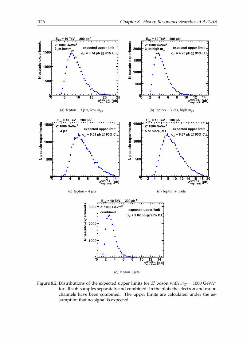
126 Chapter 8. Heavy Resonance Searches at ATLAS
(a) lepton + 3 jets, low mjet (b) lepton + 3 jets, high mjet
(c) lepton + 4 jets (d) lepton + 5 jets
(e) lepton + jets
Figure 8.2: Distributions of the expected upper limits for Z′ boson with mZ′ = 1000 GeV/c2
for all sub-samples separately and combined. In the plots the electron and muonchannels have been combined. The upper limits are calculated under the as-sumption that no signal is expected.

8.2 Sensitivity for Heavy Resonances 127
Figure 8.3: Expected upper limits at 95% CL as a function of the Z′ boson mass. Only statis-tical uncertainties have been taken into account.
The invariant mass distributions have been shown in Figure 7.8, 7.9, 7.10 and 7.11 for thebackground processes as well as for the signal with mZ′ =500, 700, 1000 and 1300 GeV/c2.
Figure 8.2 present distributions of upper limits at 95% CL for a Z′ resonance at mZ′ =1000 GeV/c2 for all sub-samples separately and combined. As expected, the “3 jet high mjet”sub-sample is most sensitive to signal. The second-best performance shows the “4 jet” sub-sample, followed by the “3 jet low mjet” and “5 or more jets” sub-sample with a similarperformance. These results are in good agreement with the performance estimate done inSection 7.4. A combination of all sub-samples provides the final result. The expected upperlimit is defined as a median of this distribution. It means, that in 50% of cases the measuredcross-section will be below the given value.
The expected upper limit on the signal cross-section taking only statistical uncertainty asa function of the resonance mass can be found in Figure 8.3. It shows upper limits for thesingle sub-samples as well as for the combination of sub-samples. The calculation is pre-pared only for resonance masses below 2000 GeV/c2, because it is the most interesting massrange at low integrated luminosity. The “3 jet low mjet” sub-sample looses on sensitivitywith the increasing Z′ boson mass. In contrast, the “3 jet high mjet” sub-sample is insensi-tive around tt mass threshold, but it has the lowest upper limit on the cross section above1000 GeV/c2. The sensitivity of “4 jet” and “5 or more jets” sub-samples is similar at massesabove 1300 GeV/c2, at lower masses we expect less signal events with additional jets.

128 Chapter 8. Heavy Resonance Searches at ATLAS
Figure 8.4: The 95% CL exclusion limits on the cross section, taking into account the mainsources of systematic uncertainty.
To estimate the effect of systematic biases and uncertainties on the sensitivity to the sig-nal, the statistical analysis is repeated including several effects, that are expected to leadto significant systematic uncertainties. The following systematic uncertainties have beenconsidered:
• an uncertainty on the jet energy scale of 10%
• the jet energy resolution is degraded by smearing the jet ET with an additional 25%√E
+5%
• 10% error on the luminosity
• 30% uncertainty on the amount of the QCD background
• PDF uncertainty
• initial and final state radiation
• top quark mass
These systematics have the largest impact on the sensitivity as discussed in Section 7.5. Theupper limits on the signal production cross-section are presented in Figure 8.4 and sum-marised in Table 8.1. The limits could be set to 3.62+1.6
−1.1 pb (mZ′ = 1000 GeV/c2), 2.16+0.9−0.7 pb
(mZ′ = 1300 GeV/c2) and 1.01+0.5−0.3 pb (mZ′ = 2000 GeV/c2) assuming
√s = 10 TeV collisions
and 200 pb−1 of integrated luminosity. At Z′ boson masses below 1000 GeV/c2, the sys-tematic uncertainties reduces significantly the sensitivity to the signal. At Z′ boson masses
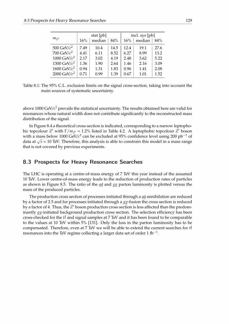
8.3 Prospects for Heavy Resonance Searches 129
mZ′stat [pb] incl. sys [pb]
16% median 84% 16% median 84%
500 GeV/c2 7.49 10.4 14.5 12.4 19.1 27.6700 GeV/c2 4.41 6.11 8.52 6.27 8.99 13.21000 GeV/c2 2.17 3.02 4.19 2.48 3.62 5.221300 GeV/c2 1.36 1.90 2.64 1.46 2.16 3.091600 GeV/c2 0.94 1.31 1.83 0.96 1.41 2.082000 GeV/c2 0.71 0.99 1.39 0.67 1.01 1.52
Table 8.1: The 95% C.L. exclusion limits on the signal cross-section, taking into account themain sources of systematic uncertainty.
above 1000 GeV/c2 prevails the statistical uncertainty. The results obtained here are valid forresonances whose natural width does not contribute significantly to the reconstructed massdistribution of the signal.
In Figure 8.4 a theoretical cross-section is indicated, corresponding to a narrow leptopho-bic topcolour Z′ with Γ/mZ′ = 1.2% listed in Table 4.2. A leptophobic topcolour Z′ bosonwith a mass below 1000 GeV/c2 can be excluded at 95% confidence level using 200 pb−1 ofdata at
√s = 10 TeV. Therefore, this analysis is able to constrain this model in a mass range
that is not covered by previous experiments.
8.3 Prospects for Heavy Resonance Searches
The LHC is operating at a centre-of-mass energy of 7 TeV this year instead of the assumed10 TeV. Lower centre-of-mass energy leads to the reduction of production rates of particlesas shown in Figure 8.5. The ratio of the qq and gg parton luminosity is plotted versus themass of the produced particles.
The production cross section of processes initiated through a qq annihilation are reducedby a factor of 2.5 and for processes initiated through a gg-fusion the cross section is reducedby a factor of 4. Thus, the Z′ boson production cross section is less affected than the predom-inantly gg-initiated background production cross section. The selection efficiency has beencross-checked for the tt and signal samples at 7 TeV and it has been found to be comparableto the values at 10 TeV within 5% [131]. Only the loss in the parton luminosity has to becompensated. Therefore, even at 7 TeV we will be able to extend the current searches for ttresonances into the TeV regime collecting a larger data set of order 1 fb−1.

130 Chapter 8. Heavy Resonance Searches at ATLAS
Figure 8.5: Parton luminosity ratio 7 TeV/10 TeV centre-of-mass at the LHC as a function ofthe mass of produced particles [132].

9 Summary and Conclusions
In this thesis a new inclusive topological multi-vertex finder, ZVTOP, was implementedin the ATLAS software framework. ZVTOP is used for the identification of B to D hadroncascades in b-jets. The main concept is to search for vertices in the three dimensional space incontrast to former algorithms which form vertices from all track combinations. Vertices arefound using a vertex probability function which is defined by the trajectories and positionresolution of the tracks. Reconstructed vertices are used as input for the b-jet identification.One method is based on a likelihood ratio approach and the second one on an artificialneural network. Using a neural network approach results in the light quark jet rejection ratefor tt events of 108 (208) with a b-tagging efficiency of 60% (50%). This means only one every108(280) light-quark jets is mis-identified as a b-jet. The relative improvement compared tothe standard algorithm is ∼ 8%. Future improvements are expected using collision datacollected by the experiment, especially in calibrating and tuning the ZVTOP tagger.
The main part of the thesis concentrates on the search for heavy narrow width resonancesin the tt invariant mass spectrum. A new reconstruction scheme has been developed forthe efficient selection and reconstruction of tt final states at various resonance masses. Thetopology of events produced at the tt mass threshold differs significantly from the eventtopology at mtt ∼ 1-2 TeV/c2. With increasing mass, the decay products of the individualtop quarks will become more collimated. The partons from W bosons or even from topquarks may be reconstructed into one jet. Such jets have a high invariant mass comparableto the mass of intrinsic quarks or bosons. The invariant jet mass is used to identify theevent topology and the topology dependent reconstruction of the mtt distribution can beperformed.
The sensitivity of the ATLAS experiment for a discovery of a narrow uncoloured tt res-onance using the presented method is encouraging: a 95% CL exclusion on the produc-tion cross-section including systematical uncertainties could be set to 3.62+1.6
−1.1 pb (mZ′ =1000 GeV/c2), 2.16+0.9
−0.7 pb (mZ′ = 1300 GeV/c2) and 1.01+0.5−0.3 pb (mZ′ = 2000 GeV/c2) as-
suming√
s = 10 TeV collisions and 200 pb−1 of integrated luminosity. So a leptophobictopcolour Z′ boson with a mass below 1000 GeV/c2 can be excluded at 95% confidence level.Therefore, this analysis is able to constrain this model in a mass range that is not covered bythe previous experiments.
Two other approaches have been developed at ATLAS to reconstruct heavy tt reso-nances [131]. The first approach performs a full reconstruction of the top and anti-topquarks. Observables like the mass of the reconstructed top quark candidates, in combi-nation with b-tagging, allow for a tight control of the reducible backgrounds. The secondapproach is designed to reconstruct highly boosted top quarks. This algorithm reconstructsthe full top quark decay as a single jet. The sensitivity of all three reconstruction methods iscomparable in the mass range around 1000 GeV/c2. At lower masses, the full reconstruction

132 Chapter 9. Summary and Conclusions
approach achieves better results due to a better background suppression. At higher masses,the mono-jet reconstruction approach is more sensitive, because the fraction of events withthe fully merged topology increases with the increasing resonance mass.
The CMS experiment at the LHC has prepared an analysis for a search for narrow widthresonances at
√s = 10 TeV and an assumed integrated luminosity of 200 pb−1 in the muon
channel only [133]. They claim an expected cross section exclusion limit at 95% CL of7.5+4.4−2.7 pb for a 1000 GeV/c2 heavy resonance and a limit of 2.9+0.5
−0.4 pb for a 2000 GeV/c2
heavy resonance. This analysis is more sensitive, because - among other differences - bothlepton channels are used.

List of Figures
2.1 Fundamental particles of the Standard Model . . . . . . . . . . . . . . . . . . . 62.2 Elements of Feynman diagrams in QCD . . . . . . . . . . . . . . . . . . . . . . 62.3 Higher order corrections to the QCD coupling αS . . . . . . . . . . . . . . . . . 72.4 Elements of Feynman diagrams in QED . . . . . . . . . . . . . . . . . . . . . . 82.5 Feynman diagrams associated with the Higgs Lagrangian term LHiggs . . . . 102.6 PDFs for u, u, d, d, s quarks and gluons inside the proton at µ = mt . . . . . . . 122.7 tt production channels at leading order perturbation theory . . . . . . . . . . 132.8 PDFs for u, u, d, d quarks and gluons inside the proton at µ = 1 TeV . . . . . . 142.9 Feynman diagrams for resonant tt production . . . . . . . . . . . . . . . . . . 162.10 Z′ boson mass distributions in the mass range 500-3000 GeV/c2 . . . . . . . . . 18
3.1 The LHC injector complex . . . . . . . . . . . . . . . . . . . . . . . . . . . . . . 203.2 View of the ATLAS detector . . . . . . . . . . . . . . . . . . . . . . . . . . . . . 223.3 Views of the ATLAS inner detector . . . . . . . . . . . . . . . . . . . . . . . . . 243.4 Pixel and SCT modules . . . . . . . . . . . . . . . . . . . . . . . . . . . . . . . . 253.5 TRT barrel and endcaps structures and modules . . . . . . . . . . . . . . . . . 253.6 Cut-away view of the calorimeter system . . . . . . . . . . . . . . . . . . . . . 263.7 Sketch of the barrel module of electromagnetic calorimeter . . . . . . . . . . . 283.8 The cumulative amounts of material in front of and in the calorimeter . . . . 303.9 Schematic view of the muon spectrometer . . . . . . . . . . . . . . . . . . . . . 313.10 Placement of the forward detectors LUCID, ZDC and ALFA . . . . . . . . . . 333.11 Expected event rates at luminosity of 1034 cm−2s−1 and
√s = 14 TeV . . . . . 35
3.12 The instantaneous and total luminosity at√
s = 7 TeV . . . . . . . . . . . . . . 37
4.1 General structure of a hard proton-proton collision . . . . . . . . . . . . . . . . 404.2 Z′ boson invariant mass distribution, rapidity y and pT distributions of top
and antitop quarks . . . . . . . . . . . . . . . . . . . . . . . . . . . . . . . . . . 47
5.1 Track helix in the transverse and in the longitudinal plane. . . . . . . . . . . . 545.2 Electron identification efficiency as a function of ET and η . . . . . . . . . . . . 585.3 Combined muon reconstruction efficiency and resolution . . . . . . . . . . . . 595.4 Illustration of infrared and collinear sensitivity . . . . . . . . . . . . . . . . . . 605.5 Illustration of signal towers and topological cell clusters . . . . . . . . . . . . 635.6 Jet reconstruction flow in ATLAS . . . . . . . . . . . . . . . . . . . . . . . . . . 645.7 Jet mass distributions at hadron colliders . . . . . . . . . . . . . . . . . . . . . 665.8 Performance of missing transverse energy reconstruction . . . . . . . . . . . . 68
6.1 Measured e+e− fragmentation function of b-quarks into B hadrons at√s ∼ 91 GeV . . . . . . . . . . . . . . . . . . . . . . . . . . . . . . . . . . . . . . 72
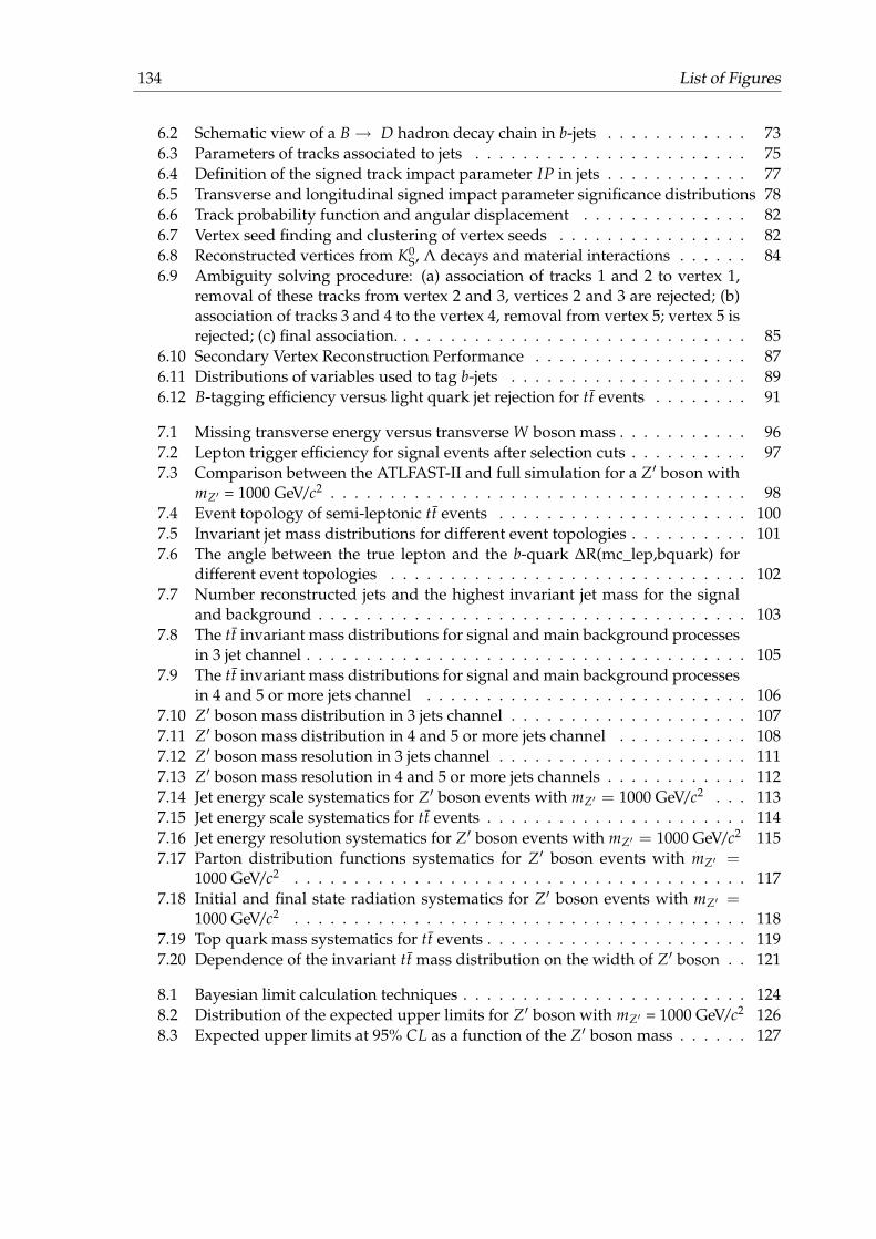
134 List of Figures
6.2 Schematic view of a B→ D hadron decay chain in b-jets . . . . . . . . . . . . 736.3 Parameters of tracks associated to jets . . . . . . . . . . . . . . . . . . . . . . . 756.4 Definition of the signed track impact parameter IP in jets . . . . . . . . . . . . 776.5 Transverse and longitudinal signed impact parameter significance distributions 786.6 Track probability function and angular displacement . . . . . . . . . . . . . . 826.7 Vertex seed finding and clustering of vertex seeds . . . . . . . . . . . . . . . . 826.8 Reconstructed vertices from K0
S, Λ decays and material interactions . . . . . . 846.9 Ambiguity solving procedure: (a) association of tracks 1 and 2 to vertex 1,
removal of these tracks from vertex 2 and 3, vertices 2 and 3 are rejected; (b)association of tracks 3 and 4 to the vertex 4, removal from vertex 5; vertex 5 isrejected; (c) final association. . . . . . . . . . . . . . . . . . . . . . . . . . . . . . 85
6.10 Secondary Vertex Reconstruction Performance . . . . . . . . . . . . . . . . . . 876.11 Distributions of variables used to tag b-jets . . . . . . . . . . . . . . . . . . . . 896.12 B-tagging efficiency versus light quark jet rejection for tt events . . . . . . . . 91
7.1 Missing transverse energy versus transverse W boson mass . . . . . . . . . . . 967.2 Lepton trigger efficiency for signal events after selection cuts . . . . . . . . . . 977.3 Comparison between the ATLFAST-II and full simulation for a Z′ boson with
mZ′ = 1000 GeV/c2 . . . . . . . . . . . . . . . . . . . . . . . . . . . . . . . . . . . 987.4 Event topology of semi-leptonic tt events . . . . . . . . . . . . . . . . . . . . . 1007.5 Invariant jet mass distributions for different event topologies . . . . . . . . . . 1017.6 The angle between the true lepton and the b-quark ∆R(mc_lep,bquark) for
different event topologies . . . . . . . . . . . . . . . . . . . . . . . . . . . . . . 1027.7 Number reconstructed jets and the highest invariant jet mass for the signal
and background . . . . . . . . . . . . . . . . . . . . . . . . . . . . . . . . . . . . 1037.8 The tt invariant mass distributions for signal and main background processes
in 3 jet channel . . . . . . . . . . . . . . . . . . . . . . . . . . . . . . . . . . . . . 1057.9 The tt invariant mass distributions for signal and main background processes
in 4 and 5 or more jets channel . . . . . . . . . . . . . . . . . . . . . . . . . . . 1067.10 Z′ boson mass distribution in 3 jets channel . . . . . . . . . . . . . . . . . . . . 1077.11 Z′ boson mass distribution in 4 and 5 or more jets channel . . . . . . . . . . . 1087.12 Z′ boson mass resolution in 3 jets channel . . . . . . . . . . . . . . . . . . . . . 1117.13 Z′ boson mass resolution in 4 and 5 or more jets channels . . . . . . . . . . . . 1127.14 Jet energy scale systematics for Z′ boson events with mZ′ = 1000 GeV/c2 . . . 1137.15 Jet energy scale systematics for tt events . . . . . . . . . . . . . . . . . . . . . . 1147.16 Jet energy resolution systematics for Z′ boson events with mZ′ = 1000 GeV/c2 1157.17 Parton distribution functions systematics for Z′ boson events with mZ′ =
1000 GeV/c2 . . . . . . . . . . . . . . . . . . . . . . . . . . . . . . . . . . . . . . 1177.18 Initial and final state radiation systematics for Z′ boson events with mZ′ =
1000 GeV/c2 . . . . . . . . . . . . . . . . . . . . . . . . . . . . . . . . . . . . . . 1187.19 Top quark mass systematics for tt events . . . . . . . . . . . . . . . . . . . . . . 1197.20 Dependence of the invariant tt mass distribution on the width of Z′ boson . . 121
8.1 Bayesian limit calculation techniques . . . . . . . . . . . . . . . . . . . . . . . . 1248.2 Distribution of the expected upper limits for Z′ boson with mZ′ = 1000 GeV/c2 1268.3 Expected upper limits at 95% CL as a function of the Z′ boson mass . . . . . . 127

List of Figures 135
8.4 The 95% CL exclusion limits on the cross section, taking into account the mainsources of systematic uncertainty . . . . . . . . . . . . . . . . . . . . . . . . . . 128
8.5 Parton luminosity ratio 7 TeV/10 TeV at the LHC . . . . . . . . . . . . . . . . . 130
List of Tables
2.1 The fields of the Standard Model and their quantum numbers . . . . . . . . . 52.2 Overview of some tt resonance benchmark models . . . . . . . . . . . . . . . . 16
3.1 General performance goals of the ATLAS detector . . . . . . . . . . . . . . . . 213.2 Granularity and number of readout channels of the ATLAS calorimeters . . . 273.3 Main parameters of the muon spectrometer . . . . . . . . . . . . . . . . . . . . 323.4 Operational fraction of ATLAS detector components . . . . . . . . . . . . . . . 37
4.1 PYTHIA parameter settings for Z′ boson couplings to fermions . . . . . . . . . 464.2 Cross section σ and width Γ as a function of the Z′ boson mass . . . . . . . . . 464.3 Generated single top quark and top quark pairs samples . . . . . . . . . . . . 484.4 Generated W + jets samples . . . . . . . . . . . . . . . . . . . . . . . . . . . . . 494.5 Generated Z + jets samples . . . . . . . . . . . . . . . . . . . . . . . . . . . . . 504.6 Generated QCD multijet samples . . . . . . . . . . . . . . . . . . . . . . . . . . 51
5.1 Expected track parameter resolutions for isolated, single muons . . . . . . . . 55
6.1 Main decay modes and some properties of B and D hadrons . . . . . . . . . . 736.2 Jet and track selection criteria for b-tagging . . . . . . . . . . . . . . . . . . . . 746.3 Average track multiplicity in b- and light jets with relative contribution of tracks 766.4 The list of tunable parameter of topological vertex finder . . . . . . . . . . . . 866.5 Light quark jet rejection for the fixed b-tagging efficiencies of 50%, 60% and
70% for tt events . . . . . . . . . . . . . . . . . . . . . . . . . . . . . . . . . . . . 91
7.1 Summary of the semi-leptonic event selection cuts . . . . . . . . . . . . . . . . 957.2 Number of expected signal and background events after the semi-leptonic
selection cuts over the whole mtt range . . . . . . . . . . . . . . . . . . . . . . . 957.3 Categorisation of selected signal events in the di-leptonic, semi-leptonic and
fully hadronic channels . . . . . . . . . . . . . . . . . . . . . . . . . . . . . . . . 997.4 Signal and background contribution in different event sub-samples . . . . . . 1047.5 Number of expected signal and background events in the ±1 RMS range
around the signal peak . . . . . . . . . . . . . . . . . . . . . . . . . . . . . . . . 1097.6 Z′ Mass Resolution . . . . . . . . . . . . . . . . . . . . . . . . . . . . . . . . . . 1107.7 Summary of the relative uncertainty on the overall normalisation . . . . . . . 120
8.1 The 95% C.L. exclusion limits on the signal cross-section . . . . . . . . . . . . 129

Bibliography
[1] S. Glashow, Nucl. Phys. 22 , 579 (1961).
[2] S. Weinberg, Phys. Rev. Lett. 19 , 1264 (1967).
[3] A. Salam, In: Elementary Particle Theory (8th Nobel Symposium, Almqvist and Wiksell,Stockholm, 1968), p. 367ff.
[4] A. Salam and J. Ward, Phys. Lett. 13 , 168 (1964).
[5] S. Glashow, J. Iliopoulos, and L. Maiani, Phys. Rev. D 2 , 1285 (1970).
[6] H. Georgi and S. L. Glashow, Phys. Rev. Lett. 28 , 1494 (1972).
[7] H. D. Politzer, Phys. Rept. 14 , 129 (1974).
[8] D. J. Gross and F. Wilczek, Phys. Rev. D 8 , 3633 (1973).
[9] G. ’t Hooft, Nucl. Phys. B 35 , 167 (1971).
[10] G. ’t Hooft and M. Veltman, Nucl. Phys. B 44 , 189 (1972).
[11] P. W. Higgs, Phys. Rev. 145 , 1156 (1966).
[12] J. Goldstone, A. Salam, and S. Weinberg, Phys. Rev. 127 , 965 (1962).
[13] E. Noether, Nachr. v. d. Ges. d. Wiss. zu Goettingen, Math-phys. Klasse, pp. 235-257,1918.
[14] Particle Data Group, K. Nakamura et al., J. Phys. G 37 , 075021 (2010).
[15] TEVATRON Electroweak Working Group, (2010), arXiv:1007.3178.
[16] T. Degrand and C. DeTar, Lattice Methods for Quantum Chromodynamics (World Scien-tific, 2006).
[17] F. Halzen and A. D. Martin, Quarks and Leptons: An Introductory Course in ModernParticle Physics. (John Wiley and Sons Inc., 1984).
[18] C. Wu, E. Ambler, R. Hayward, D. Hoppes, and R. Hudson, Phys. Rev. 105 , 1413(1957).
[19] G. Abbiendi et al., Phys. Lett. B 565 , 61 (2003).
[20] T. Aaltonen et al., Phys. Rev. Lett. 104 , 061802 (2010).
[21] N. Cabibbo, Phys. Rev. Lett. 10 , 531 (1963).
[22] M. Kobayashi and T. Maskawa, Prog. Theor. Phys. 49 , 652 (1973).
[23] Z. Maki, M. Nakagawa, and S. Sakata, Prog. Theor. Phys. 28 , 870 (1962).
[24] F. Abe et al., Phys. Rev. Lett. 74 , 2626 (1995).
[25] S. Abachi et al., Phys. Rev. Lett. 74 , 2422 (1995).

138 Bibliography
[26] S. Moch and P. Uwer, Nucl. Phys. Proc. Suppl. 183 (2008), arXiv:0807.2794.
[27] Z. Sullivan, Phys. Rev. D 70 , 114012 (2004), hep-ph/0408049.
[28] W. K. Tung, p. 1369 (1987), FERMILAB-CONF-87-122-T.
[29] J. Pumplin et al., JHEP 07 , 012 (2002), hep-ph/0201195.
[30] M. Beneke et al., (2000), hep-ph/0003033.
[31] S. Catani, D. de Florian, M. Grazzini, and P. Nason, JHEP 07 , 028 (2003), hep-ph/0306211.
[32] N. Andari et al., (2010), ATL-PHYS-INT-2010-030.
[33] K. Gaemers and F. Hoogeveen, Phys. Lett. B 146 , 347 (1984).
[34] D. Dicus, A. Stange, and S. Willenbrock, Phys. Lett. B 333 , 126 (1994), hep-ph/9404359.
[35] W. Bernreuther, M. Flesch, and P. Haberl, Phys. Rev. D 58 , 114031 (1998), hep-ph/9709284.
[36] A. Djouadi, Phys. Rept. 459 , 1 (2008), hep-ph/0503173.
[37] A. Manohar and M. Wise, Phys. Rev. D 74 , 035009 (2006), hep-ph/0606172.
[38] M. Gresham and M. Wise, Phys. Rev. D 76 , 075003 (2007), arXiv:0706.0909.
[39] I. Antoniadis, Phys. Lett. B 246 , 377 (1990).
[40] T. Rizzo and J. Wells, Phys. Rev. D 61 , 0160072 (1999).
[41] A. Leike, Phys. Rept. 317 , 143 (1999), hep-ph/9805494.
[42] J. Hewett and T. Rizzo, Phys. Rept. 183 , 193 (1989).
[43] M. Cvetic and S. Godfrey, (1995), hep-ph/9504216.
[44] T. Rizzo, (1996), hep-ph/9612440.
[45] E. Eichten and K. Lane, Phys. Lett. B 90 , 125 (1980).
[46] C. T. Hill and S. J. Parke, Phys. Rev. D 49 , 4454 (1994), hep-ph/9312324.
[47] C. T. Hill, Phys. Lett. B 345 , 483 (1995), hep-ph/9411426.
[48] L. Randall and R. Sundrum, Phys. Rev. Lett. 83 , 3370 (1999).
[49] H. Davoudiasl, J. L. Hewett, and T. G. Rizzo, Phys. Rev. Lett. 84 , 2080 (2000).
[50] CDF, T. Aaltonen et al., Phys. Rev. Lett. 102 , 091805 (2009), arXiv:0811.0053.
[51] CDF, T. Aaltonen et al., Phys. Rev. Lett. 102 , 031801 (2009), arXiv:0810.2059.
[52] V. Abazov et al., (2009), DØ note 5923-conf.
[53] CDF, T. Aaltonen et al., Phys. Rev. D 79 , 112002 (2009), arXiv:0812.4036.
[54] DØ, V. M. Abazov et al., Phys. Lett. B 668 , 98 (2008), arXiv:0804.3664.
[55] DØ, V. M. Abazov et al., (2009), DØ note 5882-CONF.
[56] CDF, T. Aaltonen et al., Phys. Rev. D 77 , 051102 (2008), arXiv:0710.5335.
[57] V. Abazov et al., (2009), DØ note 5882-conf.
[58] CDF, T. Aaltonen et al., (2008), CDF note 9164.

Bibliography 139
[59] CDF, C. Ciobanu et al., FERMILAB-FN-0773-E.
[60] S. Godfrey, Phys. Rev. D 51 , 1402 (1995).
[61] A. Leike, Phys. Lett. B 402 , 374 (1997).
[62] A. Scharf, private communication.
[63] ATLAS, G. Aad et al., JINST 3 S08003 (2008).
[64] CMS, S. Chatrchyan et al., JINST 3 S08004 (2008).
[65] LHCb, A. A. Jr et al., JINST 3 S08005 (2008).
[66] TOTEM, G. Antchev et al., Nucl. Inst. Meth. Phys. Res. 617 , 62 (2010).
[67] ALICE, K. Aamondt et al., JINST 3 S08002 (2008).
[68] L. Evans and P. Bryant, JINST 3 S08001 (2008).
[69] J.-L. Caron, The LHC Injection Complex, AC Collection, 1993.
[70] J. Pequenao, Computer Generated Images of the ATLAS Detectors, 2008.
[71] ATLAS, G. Aad et al., (1998), CERN-LHCC-98-14.
[72] ATLAS, G. Aad et al., (2003), CERN/LHCC/03-022.
[73] ATLAS, G. Aad et al., (2009), arXiv:0901.0512v4.
[74] ATLAS, G. Aad et al., (2010), arXiv:1004.5293.
[75] ATLAS, G. Aad et al., (2009), arXiv:0912.2642.
[76] ATLAS, G. Aad et al., (2010), arXiv:1006.4384.
[77] ATLAS, G. Aad et al., (2010), ATLAS-CONF-2010-060.
[78] A. Agostinelli et al., Nucl. Inst. Meth. Phys. Res. 506 , 250 (2003).
[79] ATLAS, G. Aad et al., (05/2010), arXiv:1005.4568, Submitted to Eur. Phys. J. C.
[80] M. Mangano and S. T.J., Annu. Rev. Nucl. Part. Sci. 55 , 555 (2005).
[81] M. Mangano et al., JHEP 07 , 001 (2003), hep-ph/0206293.
[82] F. Krauss, R. Kuhn, and G. Soff, J. Phys. G. 26(1) , L11 (2000), hep-ph/9904274.
[83] S. Catani, F. Krauss, B. R. Webber, and R. Kuhn, JHEP 11 , 063 (2001), hep-ph/0109231.
[84] V. Sudakov, Sov. Phys. JETP 3 , 65 (1956).
[85] S. Frixione, P. Nason, and B. Webber, JHEP 08 , 007 (2003), hep-ph/0305252.
[86] T. Sjöstrand, S. Mrenna, and P. Skands, JHEP 05 , 026 (2006), hep-ph/0603175.
[87] B. Andersson, G. Gustafson, G. Ingelman, and T. Sjöstrand, Phys. Rept. 97 , 31 (1983).
[88] G. Corcella et al., JHEP 01 , 010 (2001), hep-ph/0011363.
[89] G. Corcella et al., (2005), hep-ph/0210213, CERN-TH/2002-270.
[90] UA5, G. Alner et al., Nucl. Phys. B 291 , 445 (1987).
[91] J. Butterworth, J. R. Forshaw, and M. Seymour, Z. Phys. C72 , 637 (1996), hep-ph/9601371.
[92] ATLAS, G. Aad et al., (2010), ATLAS-CONF-2010-058.
140 Bibliography
[93] ATLAS, G. Aad et al., (2010), ATLAS-CONF-2010-019.
[94] ATLAS, G. Aad et al., (2010), ATLAS-CONF-2010-067.
[95] H. Hakobyan, M. Simonyan, T. Carli, and A. M. Henriques-Correia, (2006), ATL-TILECAL-PUB-2007-008.
[96] ATLAS, G. Aad et al., (2010), ATLAS-CONF-2010-052.
[97] ATLAS, G. Aad et al., (2010), ATLAS-CONF-2010-064.
[98] R. M. Harris, C. T. Hill, and S. J. Parke, (1999), hep-ph/9911288.
[99] A. Shibata et al., (2009), ATL-COM-PHYS-2009-334.
[100] P. Hough, Proc. Int. Conf. High Energy Accelerators and Instrumentation (1959).
[101] R. Kalman, Transaction of the ASME, Journal of Basic Engineering , 35 (1960).
[102] T. Cornelissen et al., (2007), ATL-SOFT-PUB-2007-007.
[103] G. Piacquadio, K. Prokofiev, and A. Wildauer, J. Phys. : Conf. Ser. 119 , 032033 (2008).
[104] M. Cacciari, G. Salam, and G. Soyez, http://www.lpthe.jussieu.fr/~salam/fastjet.
[105] S. Catani, Y. L. Dokshitzer, M. H. Seymour, and B. R. Webber, Nucl. Phys. B406 , 187(1993).
[106] S. D. Ellis and D. E. Soper, Phys. Rev. D 48 , 3160 (1993).
[107] M. Cacciari, G. P. Salam, and G. Soyez, JHEP 04 , 063 (2008), arXiv:0802.1189.
[108] Y. L. Dokshitzer, G. D. Leder, S. Moretti, and B. R. Webber, JHEP 08 , 001 (1997),hep-ph/9707323.
[109] M. Wobisch and T. Wengler, (1998), hep-ph/9907280.
[110] L. Asquith et al., (2009), ATL-COM-PHYS-2009-630.
[111] I. Abt et al., Nucl. Inst. Meth. A 386 , 348 (1997).
[112] U. Baur and L. H. Orr, Phys. Rev. D 76 , 094012 (2007), arXiv:0707.2066.
[113] J. Thaler and L.-T. Wang, JHEP 07 , 092 (2008), arXiv:0806.0023.
[114] L. G. Almeida et al., Phys. Rev. D 79 , 074017 (2009), arXiv:0807.0234.
[115] S. Ellis, J. Huston, K. Hatakeyama, P. Loch, and M. Tonnesmann, Prog. Part. Nucl.Phys. 60 , 484 (2008), arXiv:0712.2447.
[116] T. Chwalek, Messung der W-Boson-Helizitätsanteile in Top-Quark-Zerfällen mit dem CDFII Experiment und Studien zu einer frühen Messung des ttbar-Wirkungsquerschnitts mit demCMS Experiment, PhD thesis, 2010.
[117] V. Kostyukhin, (2003), ATL-PHYS-2003-031.
[118] V. Kostyukhin, (2003), ATL-PHYS-2003-033.
[119] D. Scott, Multivariate density estimation theory, practice, and visualization (NY Wiley, NewYork, 1992).
[120] G. Piacquadio and K. Jakobs, Identification of b-jets and investigation of the discoverypotential of a Higgs boson in the WH → lνbb channel with the ATLAS experiment, PhDthesis, Freiburg U., Freiburg, 2010.

Bibliography 141
[121] D. J. Jackson, Nucl. Inst. Meth. A 388 , 247 (1997).
[122] P. Billoir and S.Qian, Nucl. Inst. Meth. A 311 , 139 (1992).
[123] SLD, K. Abe et al., (1999), hep-ex/9907051.
[124] F. Rosenblatt, Psychological Rev. 65 , 386 (1958).
[125] A. Hoecker et al., ArXiv Physics e-prints (2007), arXiv:physics/0703039.
[126] B. Abbott et al., (2009), ATL-COM-PHYS-2009-633.
[127] A. D. Martin, R. G. Roberts, W. J. Stirling, and R. S. Thorne, Phys. Lett. B 531 , 216(2002), hep-ph/0201127.
[128] S. Jain, H. B. Prosper, and R. Schwienhorst, Statistical Methods Implemented in thePackage ’top_statistics’, DØ Note 5817, December 8, 2008.
[129] DØ, I. Bertram et al., FERMILAB-TM-2104.
[130] R. Barlow, A Guide to the Use of Statistical Methods in the Physical SciencesThe Manch-ester physics series (Wiley, 1989).
[131] ATLAS, G. Aad et al., (2010), ATL-PHYS-PUB-2010-008.
[132] W. Stirling, private communication.
[133] CMS, S. Chatrchyan et al., (2009), CMS-PAS-TOP-09-009.

A Acknowledgement
I would like to thank all people who supported me during the four years of my PhD thesis.First and foremost, I would like to thank Peter Mättig for the opportunity to work on thisresearch topic and for his constant support and encouragement. Furthermore, I would liketo acknowledge Richard Hawkings for his kind agreement to be the second referee of mythesis. Then I would like to thank my supervisor Thorsten Kuhl for all mostly fruitful, butsometimes falling on my or his deaf ears discussions. In spite of everything it was a pleasureto work with him.
I would like to thank Wolfgang Wagner and his team Dominic Hirschbühl, Philipp Sturmand Georg Sartisohn for their active support and especially for the nice analysis framework,the spider accompanies me every day in the last two years. I have learned a lot from you,many thanks for that. I would like to express my gratitude to Klaus Hamacher for his ad-vises in all topics even if he dislikes searches and prefers measurements. The 24/7 supportof our computing team makes the execution of my analysis much easier, many thanks toTorsten Harenberg and Joachim Schultes.
I always enjoyed the work and the time after work in Wuppertal or at CERN thanks tomy companions, Marisa Sandhoff, Thorsten Boek, Markus Mechtel, Yvonne Peters, Sebas-tian Fleischmann, Tobias Henss and Thorsten Schliephake. They had always a sympatheticear for me and help me with a good advise or just a cup of coffee or Gummibärchen. Manythanks to Marcello Barisonzi for his heroic action in printing my thesis at CERN.
Jens Dopke and Kathrin Becker were always my faithful companions and flatmates atCERN. Thanks for cooking, keeping me from work and extreme sightseeting. Not to forgetmy second hobby and my dear climbing Spartans. Last but not least I owe my family andmy husband a debt of gratitude for their patience and their long-term support.


