1 1 2 3 Explicit Prediction of Hail in a Long-lasting Multi-cellular Convective System in Eastern 4 China Using Multi-moment Microphysics Schemes 5 6 Liping Luo 1,2 , Ming Xue 1,2 , Kefeng Zhu 1 and Bowen Zhou 1 7 8 1 Key Laboratory of Mesoscale Severe Weather/Ministry of Education and School of 9 Atmospheric Sciences, Nanjing University, Nanjing, 210023, China 10 2 Center for Analysis and Prediction of Storms and School of Meteorology, 11 University of Oklahoma, Norman Oklahoma, USA 73072 12 13 14 15 16 17 Submitted to Journal of Atmospheric Sciences 18 October 2017 19 Revised February 2018 20 21 22 Corresponding author address 23 24 Ming Xue 25 Key Laboratory of Mesoscale Severe Weather/Ministry of Education 26 School of Atmospheric Sciences, Nanjing University, Nanjing, China, 210023, and 27 Center for Analysis and Prediction of Storms, 28 University of Oklahoma 29 Email: [email protected]30
Transcript
1
1 2
3 Explicit Prediction of Hail in a Long-lasting Multi-cellular Convective System in Eastern 4
China Using Multi-moment Microphysics Schemes 5
6
Liping Luo1,2, Ming Xue1,2, Kefeng Zhu1 and Bowen Zhou1 7
8 1 Key Laboratory of Mesoscale Severe Weather/Ministry of Education and School of 9 Atmospheric Sciences, Nanjing University, Nanjing, 210023, China 10
2 Center for Analysis and Prediction of Storms and School of Meteorology, 11 University of Oklahoma, Norman Oklahoma, USA 73072 12
13 14 15 16 17
Submitted to Journal of Atmospheric Sciences 18 October 2017 19
Revised February 2018 20 21 22
Corresponding author address 23
24 Ming Xue 25
Key Laboratory of Mesoscale Severe Weather/Ministry of Education 26 School of Atmospheric Sciences, Nanjing University, Nanjing, China, 210023, and 27
Center for Analysis and Prediction of Storms, 28 University of Oklahoma 29 Email: [email protected]
2
Abstract 31
During the afternoon of April 28, 2015, a multi-cellular convective system swept southward 32
through much of Jiangsu Province, China over about seven hours, producing egg-sized hailstones 33
on the ground. The hailstorm event is simulated using the Advanced Regional Prediction System 34
(ARPS) at 1-km grid spacing. Different microphysics schemes are used predicting one, two, and 35
three moments of the hydrometeor particle size distributions (PSDs). Simulated reflectivity and 36
maximum estimated size of hail (MESH) derived from the simulations are verified against 37
reflectivity observed by operational S-band Doppler radars and radar-derived MESH, respectively. 38
Comparisons suggest that the general evolution of the hailstorm is better predicted by the three-39
moment scheme, and neighborhood-based MESH evaluation further confirms the advantage of 40
three-moment scheme in hail size prediction. 41
Surface accumulated hail mass, number and hail distribution characteristics within simulated 42
storms are examined across sensitivity experiments. Results suggest that multi-moment schemes 43
produce more realistic hail distribution characteristics, with the three-moment scheme performing 44
the best. Size-sorting is found to play a significant role in determining hail distribution within the 45
storms. Detailed microphysical budget analyses are conducted for each experiment, and results 46
indicate that the differences in hail growth processes among the experiments can be mainly ascribed 47
to the different treatments of the shape parameter within different microphysics schemes. Both the 48
differences in size sorting and hail growth processes contribute to the simulated hail distribution 49
differences within storms and at the surface. 50
3
1. Introduction 51
Hailstorms are among the costliest natural disasters in China and many other countries; 52
hailstorms can cause severe injuries and extensive property damage. According to the Yearbooks of 53
Meteorological Disasters in China (e.g., 2013, 2014 and 2015), hail damages amount to billions of 54
U.S. dollars annually in China. Improving the prediction of hail, including the size and number of 55
hailstones, and the spatial and temporal coverage of hailfall, can help mitigate the impacts of 56
hailstorms through improved warnings. However, the prediction of hailstorms using operational 57
numerical weather prediction (NWP) models remains a challenge. The explicit prediction of hail at 58
the surface, including the spatial and temporal coverage of hailfall and the hail size distributions, is 59
even more challenging because of the complex microphysical as well as dynamic and 60
thermodynamic processes involved in hail production (Snook et al. 2016, Labriola et al. 2017). 61
Our general ability to forecast hail in operational and research settings is still limited (Moore 62
and Pino 1990; Brimelow et al. 2002; Guo and Huang 2002; Milbrandt and Yau 2006a, 2006b, 63
hereafter MY06a, MY06b; Brimelow and Reuter 2009; Luo et al. 2017, hereafter L17; Labriola et 64
al. 2017). Existing hail forecast methods include the following four types: i) hail diagnostics based 65
on observed soundings, ii) methods using a simple cloud model combined with a hail growth model 66
(e.g., HAILCAST) (Brimelow et al. 2002), iii) statistical and machine learning (ML) hail forecast 67
methods (e.g., random forests, gradient boosting trees, and linear regression), and iv) predictions 68
using convective-scale NWP models with sophisticated microphysics schemes. 69
For sounding-based hail diagnostic methods, the most important limitation is the lack of 70
4
timely soundings. HAILCAST addresses this issue by feeding prognostic model soundings into a 71
time-dependent hail growth model (Brimelow et al. 2002; Adams-Selin and Ziegler 2016). Gagne et 72
al. (2014) statistically validated the hail size and probability forecast skills of ML techniques and 73
HAILCAST, based on 12 hail days from May to June 2014 over the United States, and found that 74
the ML techniques produced smaller size errors compared to HAILCAST, and that both approaches, 75
especially HAILCAST, tended to overpredict the maximum hail size. ML methods also showed 76
temporal and spatial offsets with observed hailstorms (Gagne et al. 2014). 77
Since sophisticated, multi-moment microphysics parameterization (hereafter MP) schemes 78
in storm-scale NWP models are capable of predicting hydrometeor size distributions within realistic 79
environments, efforts to simulate and predict real hailstorms have been attempted using NWP 80
models in recent years (e.g., MY06a, b; Noppel et al. 2010; Snook et al. 2016; L17). For example, 81
MY06a conducted simulations of a supercell hailstorm that occurred in Canada, using the three-82
moment Milbrandt and Yau (hereafter MY) scheme in a mesoscale NWP model. Comparisons with 83
radar observations indicated that the typical supercell structures such as the hook echo, 84
mesocyclone, and suspended overhang region were well reproduced, although the simulated 85
maximum hail size on the ground was underpredicted. Snook et al. (2016) is a more recent example, 86
which evaluated short-term ensemble forecasting of hail for a supercell storm over central 87
Oklahoma using a two-moment MP scheme. They noted that hail prediction might be improved by 88
using more advanced MP schemes, especially via better explicit prediction of the properties of 89
rimed ice. 90
5
In the bulk MP schemes typically used in NWP models, the PSD of each hydrometeor 91
category is assumed to have a Marshall-Palmer or Gamma distribution, and normally one, two, or 92
three moments of the distribution are predicted for each hydrometeor category. One-moment 93
schemes typically predict only the mixing ratios (Q) of various hydrometeors (e.g., Lin et al. 1983; 94
Kessler 1995). Two-moment schemes predict the mixing ratios (Q) and total number concentrations 95
(Nt) of all or some of the hydrometeors (e.g., Ferrier 1994; Walko et al. 1995; Meyers et al. 1997; 96
Thompson et al. 2004; Milbrandt and Yau 2005a, hereafter MY05a; Morrison et al. 2005; Morrison 97
and Gettelman 2008; Thompson et al. 2008). To make the Gamma distribution (involving three free 98
parameters) fully prognostic, Milbrandt and Yau (2005b) (hereafter MY05b) proposed a three-99
moment scheme by adding a predictive equation for radar reflectivity factor (Z) of the hydrometeors 100
[related to the sixth moment] to their two-moment scheme. 101
However, many studies have noted that different bulk MP schemes often produce large 102
differences in various aspects of the simulated storms, including the storm structure, surface 103
accumulated precipitation, and cold pool (e.g., Gilmore et al. 2004; MY06b; Seifert et al. 2006; 104
Morrison et al. 2009; Dawson et al. 2010; Jung et al. 2010; Van Weverberg et al. 2012; Loftus and 105
Cotton 2014b; L17). Most of the prior studies have used idealized frameworks, in which the storm 106
environment is horizontally homogeneous, with MY06b, Snook et al. (2016), and L17 being the 107
exceptions. MY06b performed sensitivity experiments of a supercell hailstorm in Canada using 108
different MP schemes. They noted dramatic improvements in the storm structure and the predicted 109
precipitation when switching from a one-moment to a two-moment scheme. More recently, L17 110
6
investigated hail forecast skill using various MP schemes for a pulse-type hailstorm in eastern 111
China. They compared simulated total precipitation and maximum estimated size of hail (MESH) 112
(Witt et al. 1998) swaths against observations and found that the three-moment MY scheme 113
produced the best forecast. 114
Hail damage is not simply a function of maximum hail size; cumulative hail mass and 115
number concentration are also important factors (Changnon 1999; Gilmore et al. 2004). Therefore, 116
hail size distribution, cumulative mass, and number concentration predicted by various MP schemes 117
are also worth evaluating in addition to MESH. Moreover, to more robustly evaluate and document 118
the performances and behaviors of different MP schemes, and at the same time to achieve a better 119
understanding of hail production and growth processes, more studies using real data for diverse 120
types of hailstorms that may occur in different storm environments are still needed. Among the 121
existing real case studies that attempt explicit hail prediction to different degrees, MY06b and 122
Snook et al. (2016) dealt with supercell storms while L17 dealt with a pulse-type storm. To our 123
knowledge, there has not been a real-case study that focuses on the multi-cellular type of hailstorm 124
that may organize into mesoscale convective systems (MCSs). 125
In this study, explicit hail prediction of a long-lasting multi-cellular hailstorm event that 126
occurred on April 28, 2015 in eastern China is investigated. On that day, the multi-cellular 127
hailstorms swept southward through most of Jiangsu Province, China over about seven hours, 128
producing egg-sized hailstones with diameters of around 20-50 mm on the ground. As in L17, this 129
study employs the ARPS model (Xue et al. 2000, 2001, 2003). Simulation experiments are run at a 130
7
1 km horizontal grid spacing (instead of 3 km in L17) using one, two, and three-moment MY MP 131
schemes. The goals of this study are two-fold. First, the explicit hail forecast skill with different MP 132
schemes, in terms of surface hailstone size distribution, cumulative hail mass, and number 133
concentration, are evaluated. Secondly, combined with diagnostic analyses on microphysical terms, 134
the reasons for the hail forecast differences between various MP schemes are explored. Surface 135
accumulated precipitation, MESH, cumulative hail mass and number concentration are examined 136
and objective MESH evaluation is performed using the fractions skill score (FSS) “neighborhood” 137
technique (Ebert 2009). 138
The rest of this paper is organized as follows. In section 2, an overview of the 28 April 2015 139
multi-cellular hailstorm event is given. The ARPS model setup and hail forecast evaluation metrics 140
are described in sections 3 and 4, respectively. Section 5 compares the explicit hail predictions 141
using different MP schemes, and investigates the causes of such differences. Finally, a summary 142
and conclusions are presented in section 6. 143
2. Case overview 144
Hailstorms and other forms of severe weather events in the northeastern Asian Pacific 145
coastal regions including eastern and northeastern China are often associated with upper 146
troposphere cut-off lows (COLs) (Tao et al. 1980; Nieto et al. 2005, 2008; Zhang et al. 2008). Most 147
COLs occur over the northeastern part of China and often move southeastward to the coastal region 148
of Eastern China (Hu et al. 2010). The COLs can persist for several days and produce high 149
convective instability. The hailstorm studied here occurred during this type of synoptic situation, 150
8
where an upper-level COL swept from north to south across Jiangsu Province in eastern China, 151
producing severe hail. According to the Severe Weather Reports of the Chinese Meteorological 152
Administration (Fig. 1), parts of Shandong Province, north of Jiangsu, were first hit by intense small 153
size hailstones (<10 mm) in the morning (around 0900 LST). In the afternoon, multi-cellular 154
hailstorms formed along the west border of Jiangsu Province and produced a large number of egg-155
sized hailstones on the ground with the maximum observed size being ~10 cm in Yizheng City, 156
Jiangsu Province. The hailfall from these storms extended through the western part of Jiangsu 157
Province from north to south, and hail fall was continuous for as long as seven hours from around 158
0700 through 1400 UTC. In addition, intense lighting and damaging surface winds (~ 23 m s-1) 159
were also reported. 160
The multi-cellular hailstorms were observed by multiple operational S-band Doppler radars, 161
including those at Jinan, Xuzhou, Bengbu, Yancheng, Nanjing, and Nantong (see Fig. 1). Figure 2 162
presents the composite (column maximum) reflectivity from these radars. The lifespan of this long-163
lasting multi-cellular hailstorm system can be characterized by two episodes. In the first episode, a 164
series of multi-cellular hailstorms was initiated and the storms intensified along the northwest 165
border of Jiangsu Province. The storms organized into a northwest-southeast line and moved 166
southeastward (Figs. 2a, b). In the second episode, from 1100 UTC onwards, as the hailstorms 167
moved southeastward the line gradually evolved into a bow-shaped echo, with the middle portion of 168
the line bulging eastward (Figs. 2c-f). By 1400 UTC, the apex of the bow had almost reached the 169
southeast corner of Jiangsu, while the southern portion of the bow was oriented from east to west 170
9
near the southern border of Jiangsu, with its western tail extending well into Anhui Province (Fig. 171
2f). The system started to weaken 1400 UTC. At all times shown, observed reflectivity exceeds 60 172
dBZ within some of the storm cells (Fig. 2). 173
The synoptic patterns associated with this event are shown in Fig. 3. At 0600 UTC (1400 174
LST) 28 April, the northeastern coastal regions of China were beneath a deep, positively-tilted, 175
semi-permanent upper-level East Asian trough (EAT). The East-Asia upper-tropospheric jet stream 176
(EAJS) was located at the southern periphery of the trough (Fig. 3a). The jet core over land was 177
located at ~30oN and 120oE, with a maximum wind exceeding 50 m s-1 (Fig. 3a). Jiangsu Province 178
(solid red line in Fig. 3a) was located ahead of the EAT and underneath the front-left (more so at 179
earlier times) exit region of the EAJS, where favorable positive vorticity advection from the EAT 180
and the upper-level divergence near the front-left EAJS exist region acted together to destabilize the 181
atmosphere. Moreover, as seen in Figs. 3b-d, from middle to low altitude, two COLs (denoted ‘C’) 182
were embedded within the EAT, with one over the eastern coast of China and the other over the 183
East China Sea. 184
Strong cold advection is found southeast of the western COL at the 500 hPa (Fig. 3b) 185
directly over Jiangsu Province. At the 850 hPa (Fig. 3b) and at the surface (Fig. 3d), a prominent 186
convergence line is present between the two cyclonic circulations; this convergence line is also the 187
convergence boundary between the warm (temperature > 28oC) unstable (CAPE reaching 1500 J kg-188
1) air mass from the southwest that is partly associated with the southern part of the western 189
cyclonic circulation, and the much colder air (< 16 oC) with no CAPE from the northeast that is part 190
10
of the eastern cyclone. The two low-level cyclones are responsible for setting up a strong 191
convergence zone and moderately high CAPE in the air south of the convergence line. The 192
convergence forcing, coupled with the destabilizing upper-level circulations, creats an environment 193
favorable for intense deep convection. 194
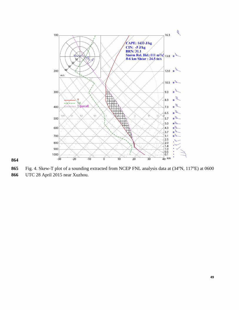
Because of the lack of observed soundings near the time of hailstorm initiation, a sounding 195
is extracted at 0600 UTC from the NCEP GFS 1o×1o Final Analysis (FNL) at (34oN, 117oE), which 196
is about 30 km southwest of Xuzhou (see Fig. 1). The hailstorm firstly initiates near Xuzhou 197
approximately one hour later at around 0700 UTC. The sounding (Fig. 4) has a CAPE of 1433 J kg-1 198
and a convective inhibition of -5 J kg-1. The situation is characterized by strong vertical wind shear, 199
with southeasterly winds below 850 hPa, and southwesterly to northwesterly winds within the 200
layers above. The bulk Richardson number is 31.1 and the 0-6 km vertical wind shear is ~24.5 m s-1; 201
these values are generally considered conducive for long-lasting severe convection (Weisman and 202
Klemp 1984). A capping inversion is present between 850 and 800 hPa; this inversion is sufficiently 203
weak that it can be overcome by strong low-level convergence while convection is generally 204
suppressed elsewhere, a situation favoring concentrated, intense deep convection. Above the 205
inversion, the air mass is dry and cold, which may be a result of the previously mentioned cold 206
advection. Many previous studies (e.g., Costa et al. 2001; L17) have noted that a dry mid-level layer 207
over a warm moist layer near the surface is favorable for larger hailstones reaching the surface due 208
to reduced melting of hail under such conditions. We note that there are uncertainties involved with 209
extracting a sounding from the FNL analysis dataset, however this sounding represents the best 210
11
available source of information about local environmental conditions. Overall, the sounding 211
indicates a conducive environment for deep convection, and a high likelihood for the production of 212
large hailstones. 213
3. Experiment setup 214
The Jiangsu hailstorm is simulated using the ARPS model (Xue et al. 2000, 2001, 2003). 215
ARPS is a three-dimensional, non-hydrostatic compressible model using generalized terrain-216
following coordinates and was designed for regional to storm-scale atmospheric modeling and 217
prediction. All simulations are initialized at 0000 UTC on 28 April 2015 and are run for 16 hours. 218
The initial condition and boundary conditions at six-hour intervals are obtained from the NCEP 219
Final Analysis data at 1o×1o resolution. 220
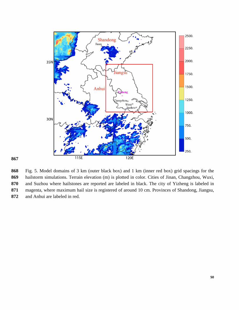
Two one-way nested grids at horizontal grid spacings of 3 and 1 km are used (Fig. 5). The 3-221
km domain covers an area of 1200×1200 km2 and is centered at (32.5oN, 118.5oE). The 1-km 222
domain is 460×460 km2 in size and covers almost all of Jiangsu Province. Both domains have 53 223
vertical levels, which are stretched using a hyperbolic tangent function as described in Xue et al. 224
(1995), with vertical grid spacing varying from 50 m at the surface to nearly 1000 m at the model 225
top; the average vertical grid spacing is 500 m. The upper and lower boundaries are set as rigid 226
walls and a two-layer soil model is applied to facilitate the calculations of surface fluxes based on 227
the predicted surface temperature and soil moisture content. Sub-grid scale turbulent mixing is 228
parameterized using a 1.5-order turbulence kinetic energy (TKE) scheme and radiative processes 229
are parameterized via the NASA Goddard Space Flight Center long- and short-wave radiation 230
12
schemes. Fourth-order advection is used in both horizontal and vertical directions, and fourth-order 231
computational mixing is applied to suppress numerical noise. More details on the ARPS physics 232
schemes and their settings can be found in Xue et al. (2001, 2003), together with the references for 233
the parameterization schemes. 234
As noted by previous studies (e.g., Loftus et al. 2014a; Snook et al. 2016; L17), hail forecast 235
errors are closely tied to uncertainties within MP schemes. Herein, simulations are conducted using 236
the MY one-, two-, and three-moment schemes (MY05a, b). Morrison and Milbrandt (2010) 237
showed that even two very similar 2-moment MP schemes could produce distinct differences in 238
simulated storms due to differences in details of the schemes. For this reason, we choose to limit 239
ourselves to the comparison of MY schemes having the same treatment of microphysical processes 240
but predicting different numeber of moments or diagnosing one of the DSD parameters. This way, 241
focus is placed on the effects of the number of predicted moments on hail forecast. In the MY 242
schemes, six distinct hydrometeor categories, i.e., cloud water, cloud ice, rain, snow, graupel, and 243
hail, are included. The PSD of each hydrometeor is represented by a gamma distribution function, 244
( ) exp( )xx 0x xN D N D Dα λ= − (1) 245
where ( )xN D is the total number concentration per unit volume of diameter D for hydrometer 246
category x. xα is the shape parameter, giving a measure of the spectral width. 0xN and xλ are the 247
intercept and slope parameters, respectively. 248
The three-moment scheme is used as the control experiment, and three other experiments are 249
performed using the one- and two-moment MY schemes. Table 1 summarizes the key parameters of 250
13
all experiments. Two of the simulations called FixA and DiagA use variants of the MY two-251
moment schemes with different treatment of the shape parameter. FixA sets the shape parameter to 252
a default constant value of 0 for all hydrometeor categories, while in DiagA the shape parameters of 253
hail and other hydrometeors are diagnosed from the mean-mass diameter of the corresponding 254
categories based on the Eqs. (12) and (13) of MY05a. The one-moment MY scheme is also tested 255
with intercept and shape parameters set to their default constant values. The above configurations 256
are similar to those of L17, except for the inclusion of the 1 km nested grid. Because 1-km grid is 257
expected to simulate the hailstorm better, we focus on results of 1-km grid in this paper. We also 258
examined the forecasts from the 3-km grid; the dominant cells simulated on the two grids are found 259
to be generally similar, although some differences exist in storm intensity at small scales. 260
4. Evaluation metrics for hail prediction 261
Three metrics for explicit hail prediction are used to evaluate hail forecast skill for the 262
various MP schemes within the sensitivity experiments. They are: maximum estimated hail size 263
(MESH) (Witt et al. 1998), maximum hail size (Dmax) (MY06a), and surface accumulated hail 264
number concentration (SAHNC). In addition, an objective neighborhood-based evaluation 265
technique, the fractions skill score, is used to verify the simulated MESH against the radar-derived 266
counterpart. L17 examined the accumulated surface precipitation and MESH fields based on the 267
simulations of a pulse-hailstorm, but not the Dmax and SAHNC. MESH and Dmax were also 268
examined in Snook et al. (2016) for a supercell storm case. 269
14
a. Maximum estimated hail size (MESH) 270
As described in L17, the MESH algorithm uses a weighted integration of radar reflectivity 271
exceeding 40 dBZ above the melting level to obtain an estimate of the maximum size of hail 272
occurring at the surface. Following L17, reflectivity datasets from multiple radars are interpolated to 273
the model grid to derive MESH. Since the MESH algorithm was only configured for hail sizes 274
larger than 19 mm (Witt et al. 1998), and Cintineo et al. (2012) and L17 only evaluated MESH 275
down to the size of 21 and 19 mm respectively, MESH values below 20 mm are excluded in this 276
study. More details about the MESH algorithm can be found in L17. 277
We note that since the MESH algorithm relies entirely upon the weighted integration of 278
radar reflectivity exceeding 40dBZ above the 0oC level to estimate hail size at the surface, there 279
may exist some biases within the derived MESH swath (e.g., Cintineo et al. 2012; Ortega et al. 280
2009). Because no other high quality/high-resolution observation of hail size is available, herein we 281
choose to use the high-resolution radar-derived MESH for verification of the hail simulations. 282
b. Maximum hail size (Dmax) 283
The maximum hail size (Dmax) (MY06a) is defined as the largest hail size for which the total 284
number concentration of hail particles greater than a diameter is equal to pre-specified total number 285
concentration, NTHRE. For example, if Dmax is 40 mm, the total number concentration of hailstones 286
larger than 40 mm is NTHRE. The Dmax parameter serves to identify the instantaneous presence of 287
large hail within the storm. Following MY06a, a threshold value of NTHRE = 10-4 m-3 is adopted here. 288
15
c. Surface accumulated hail number concentration (SAHNC) 289
Given that the accumulated hail number is also important for hail prediction, SAHNC is 290
proposed as a new parameter to estimate the surface accumulated number concentration of hail 291
larger than a particular size. The SAHNC parameter is not only useful for identifying the surface 292
accumulated hail size distribution, but also helpful in understanding storm evolution. SAHNC is 293
defined as an integration of the flux of large hail ( )hR D at 60-second intervals during hailfall from 294
T0 to T1, 295
* *( ) ( )Dh hDN D N D dD
∞= ∫ (2) 296
( ) h hb fh hV D a D eγ −= × × (3) 297
( ) ( ) ( )h h hR D N D V D= × (4) 298
1
0
( ) ( )T
hTSHNAC D R D dt= ∫ (5) 299
where ( )DhN D is the total number concentration of hail larger than diameter D, and the size 300
distribution of hail is described by gamma distribution function as equation (1). Terminal fall 301
velocity at the surface for a hailstone with diameter D is given by Eq. (3), where 1
20( )ργ ρ= is 302
the density correction factor with 0ρ and ρ being the surface air and air density; ha , hb , and hf are 303
set to be 206.89, 0.6384, and 0.0, respectively following Ferrier (1994). 304
d. Neighborhood-based hail forecast evaluation 305
As reviewed in Casati et al. (2010), evaluation of forecasts from high-resolution models has 306
been a subject of active research in recent years, and various evaluation metrics have been 307
16
developed. Objective evaluation of hail forecasts is still very challenging, partly due to the lack of 308
high-quality, high-resolution hail observations (Snook et al. 2016). In this study, the fractions skill 309
score (FSS) neighborhood technique (Roberts and Lean 2008), is applied to MESH fields derived 310
from multiple radar observations and the simulations to examine hail size forecast skill using 311
different MP schemes. Distinct from traditional point-by-point evaluation techniques, FSS 312
compares fractional coverage of forecasts against that of observations within a neighborhood 313
centered at each grid point. By varying the neighborhood size and the MESH threshold, scale-314
dependent forecast skill can be assessed. Following Roberts and Lean (2008), FSS is defined as 315
2 2
( ) O( )1 1
11 N N
F i is si i
FBSFSSP P
N = =
= − + ∑ ∑
(6) 316
where FBS is the fractional Brier score, given as 317
( )2
( ) o( )1
1 N
F i is si
FBS P PN =
= −∑ (7) 318
In Eqs. (6) and (7), N is the total number of grid boxes in the predefined neighborhood 319
(within a given radius); PF(i) and PO(i) are the fractional areas at the ith neighborhood of forecast and 320
observation, respectively. They are analogous to the probability that a given neighborhood contains 321
values larger than the pre-specific threshold. Therefore, FSS compares fractional coverage over a 322
neighborhood of given size, rather than values at each grid box, and FSS values range from 0 to 1. 323
A score of 1 signifies a forecast perfectly matching the observation within a specific neighborhood 324
for a given intensity threshold, while 0 signifies a complete mismatch. A forecast is considered to 325
17
be skillful when the FSS value exceeds FSSuseful, which is defined as (Roberts and Lean 2008), 326
0.52obs
usefulfFSS = + (8) 327
where obsf is an average of observed fraction within the entire domain. By calculating FSS at a 328
variety of spatial scales (neighborhood sizes) and MESH thresholds, one can determine how the 329
forecast skill varies with spatial scale and at which scale a forecast has useful skill for a given 330
MESH threshold. 331
5. Results 332
In this section, results of the simulations are presented. First, to validate the simulations of 333
the multi-cell hailstorm system, simulated composite (column-maximum) radar reflectivity is 334
compared with corresponding radar observations. Explicit hail forecast skills using various MP 335
schemes are then evaluated, in terms of MESH, surface accumulated solid water mass, and SAHNC. 336
Neighborhood-based FSSs for simulated MESH are calculated against radar-derived MESH. The 337
differences in hail distribution characteristics within storms simulated using different MP schemes 338
are also investigated. To understand the reasons behind the differences among various MP schemes 339
for hail prediction, microphysical budget analyses are performed. 340
a. Simulated storm evolution 341
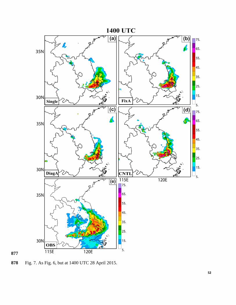
As discussed in section 2, the lifespan of this multi-cellular hailstorm can be characterized 342
by two episodes between 0700 and 1400 UTC on April 28, 2015. Figures 6 and 7 show simulated 343
composite reflectivity fields from the experiments and radar observations from one time during each 344
episode, at 0900 and 1400 UTC, respectively. Comparisons with the radar observations (Figs. 6e, 7e) 345
18
indicate that the time and location of the hailstorm’s initiation along the northwest border of Jiangsu 346
Province, as well the later organization into a large bow-shaped echo are well reproduced in the 347
simulations (Figs. 6a-d, 7a-d). The direction of movement of the simulated storms is also in general 348
agreement with observations. 349
Although the storms’ evolution and motion are generally reproduced quite well in the 350
simulations, there exist significant storm intensity differences among the experiments using various 351
MP schemes. Experiment Single under-predicts the reflectivity magnitude, having few instances of 352
reflectivity exceeding 60 dBZ, and the stratiform precipitation region (<35 dBZ) in Single is larger 353
compared to simulations using multi-moment schemes (Figs. 6a, 7a). This result differs from those 354
of some previous studies (e.g., Morrison et al. 2009, Bryan and Morrison 2012, Baba and Takahashi 355
2014); their studies noted that the stratiform precipitation region in idealized two-dimensional 356
squall line simulations was smaller using a one-moment than a two-moment scheme and they 357
attributed it to decreased rain evaporation rates in the 2-moment schemes in the trailing stratiform 358
region. In our hailstorm case, it is believed that for the multi-moment scheme, the size-sorting 359
mechanism may allow larger sized hailstones to fall rapidly towards the ground, giving less time for 360
hail mass advection downwind of the updraft and hence the smaller stratiform precipitation region. 361
This may be one of the reasons at least. 362
The reflectivity magnitudes from the multi-moment schemes are more or less over-predicted 363
when compared with radar observations (Figs. 6b-e, 7b-e). Thus, storm intensities produced by the 364
multi-moment schemes are not too different based on radar reflectivity, while the hail prediction 365
19
skill of each scheme exhibits significant discrepancies (see Figs. 8-12). Moreover, in all cases, the 366
westward extension of the reflectivity towards Anhui Province is under-predicted, and the simulated 367
system exhibits slower southward movement (possibly due to uncertainties in the initial condition), 368
resulting in the entire system being displaced almost 80 km northward compared to the observations 369
by 1400 UTC. 370
b. Hailstone forecast and evaluation 371
As the main goal of this study is to evaluate the hail forecast skills of various MP schemes, 372
predicted hail size distribution features, including hailstone size, mass, and number concentration 373
will be examined in this section. 374
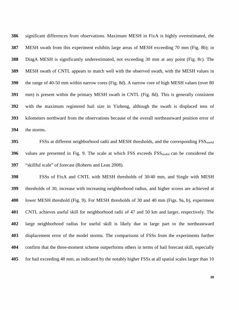
1) Radar-based hail forecast evaluation using MESH 375
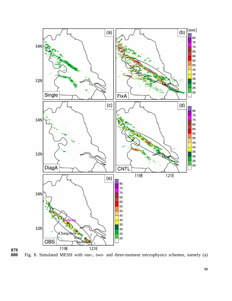
Swaths of MESH derived from the forecasts and from radar observations between 0600 and 376
1600 UTC at 5-minute intervals are presented in Fig. 8. There is one primary, nearly continuous 377
MESH swath in the radar observations (Fig. 8e), with MESH values exceeding 40 mm in many 378
locations. Along the radar-indicated MESH swath, egg-sized hailstones (with diameters of 20-50 379
mm) were reported in several cities, including Yizheng, Changzhou, Wuxi, and Suzhou. Among 380
them, maximum MESH values exceed 80 mm over Yizheng, which coincides with the location of 381
largest hail reported during this storm-a report from Yizheng of hail over 100 mm in diameter. 382
Compared with radar-derived MESH, the MESH swath derived from experiment Single exhibits 383
smaller maximum hail sizes, with several scattered cores of MESH values of no more than 35 mm 384
predicted (Fig. 8a). In FixA and DiagA, which use two-moment schemes, MESH swaths exhibit 385
20
significant differences from observations. Maximum MESH in FixA is highly overestimated, the 386
MESH swath from this experiment exhibits large areas of MESH exceeding 70 mm (Fig. 8b); in 387
DiagA MESH is significantly underestimated, not exceeding 30 mm at any point (Fig. 8c). The 388
MESH swath of CNTL appears to match well with the observed swath, with the MESH values in 389
the range of 40-50 mm within narrow cores (Fig. 8d). A narrow core of high MESH values (over 80 390
mm) is present within the primary MESH swath in CNTL (Fig. 8d). This is generally consistent 391
with the maximum registered hail size in Yizheng, although the swath is displaced tens of 392
kilometers northward from the observations because of the overall northeastward position error of 393
the storms. 394
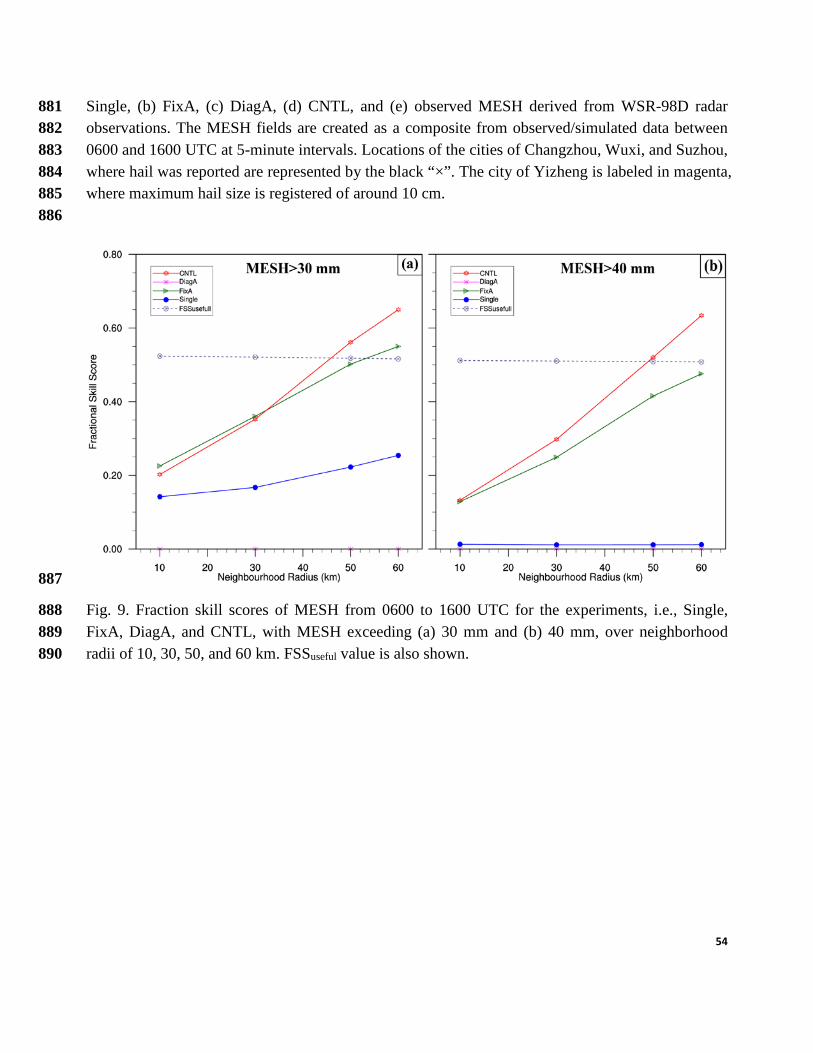
FSSs at different neighborhood radii and MESH thresholds, and the corresponding FSSuseful 395
values are presented in Fig. 9. The scale at which FSS exceeds FSSuseful can be considered the 396
“skillful scale” of forecast (Roberts and Lean 2008). 397
FSSs of FixA and CNTL with MESH thresholds of 30/40 mm, and Single with MESH 398
thresholds of 30, increase with increasing neighborhood radius, and higher scores are achieved at 399
lower MESH threshold (Fig. 9). For MESH thresholds of 30 and 40 mm (Figs. 9a, b), experiment 400
CNTL achieves useful skill for neighborhood radii of 47 and 50 km and larger, respectively. The 401
large neighborhood radius for useful skill is likely due in large part to the northeastward 402
displacement error of the model storms. The comparisons of FSSs from the experiments further 403
confirm that the three-moment scheme outperforms others in terms of hail forecast skill, especially 404
for hail exceeding 40 mm, as indicated by the notably higher FSSs at all spatial scales larger than 10 405
21
km (Fig. 9b). Experiment Single has no skill at any spatial scale for hailstones larger than 40 mm, as 406
indicated by the zero FSSs at all neighborhood radii (Fig. 9b). Similarly, DiagA shows no skill for 407
predicting hailstones larger than 30 mm (Fig. 9a). 408
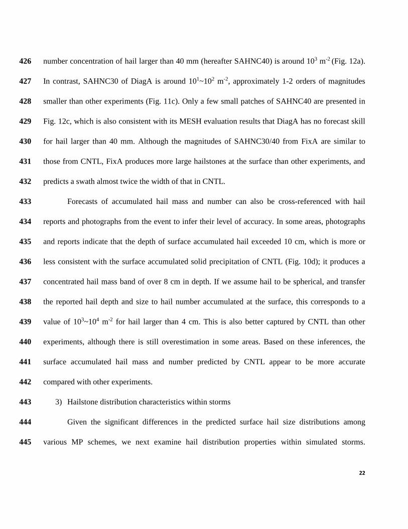
2) Surface accumulated hail mass and number concentration 409
Since there are no in-situ hail-count observations, the simulated hail mass and number 410
concentration fields are compared among the experiments in light of the registered hail reports. 411
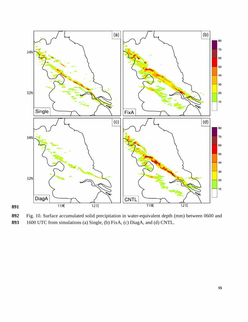
Surface accumulated hail mass fields from the experiments, calculated between 0600 and 1600 412
UTC throughout almost entire lifespan of the hailstorm are shown in Fig. 10. The corresponding 413
SAHNC, derived from the model output within the same period at 60-second intervals for hail 414
diameter thresholds of 30 and 40 mm, are shown in Figs. 11 and 12. 415
The storms in Single produce a northwest-southeast-oriented swath of hail mass, with peak 416
values of around 80 mm, mainly concentrated within a narrow band approximately 10 km in width 417
(Fig. 10a). In DiagA, the accumulated hail mass amounts are the smallest among all experiments, 418
with peak values below 40 mm (Fig. 10c). The width of the primary hail mass swath in FixA is the 419
widest (around 20 km) among the experiments. Peak values in FixA and CNTL are similar (~80 420
mm), and the hail mass predicted by CNTL appears to be more concentrated along a relatively 421
straight path (Fig. 10d). 422
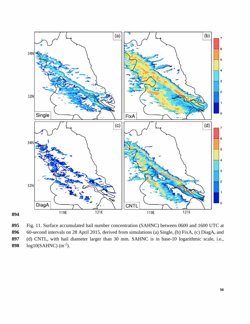
Distributions of SAHNC from the experiments generally coincide with their hail mass 423
distributions. For example, SAHNC of Single with hail size larger than 30 mm (hereafter 424
SAHNC30) within the primary narrow hail mass band is around 104~105 m-2 (Fig. 11a), and the 425
22
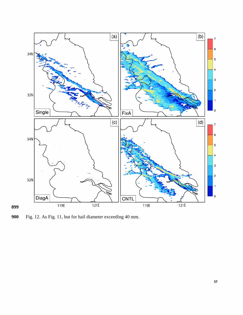
number concentration of hail larger than 40 mm (hereafter SAHNC40) is around 103 m-2 (Fig. 12a). 426
In contrast, SAHNC30 of DiagA is around 101~102 m-2, approximately 1-2 orders of magnitudes 427
smaller than other experiments (Fig. 11c). Only a few small patches of SAHNC40 are presented in 428
Fig. 12c, which is also consistent with its MESH evaluation results that DiagA has no forecast skill 429
for hail larger than 40 mm. Although the magnitudes of SAHNC30/40 from FixA are similar to 430
those from CNTL, FixA produces more large hailstones at the surface than other experiments, and 431
predicts a swath almost twice the width of that in CNTL. 432
Forecasts of accumulated hail mass and number can also be cross-referenced with hail 433
reports and photographs from the event to infer their level of accuracy. In some areas, photographs 434
and reports indicate that the depth of surface accumulated hail exceeded 10 cm, which is more or 435
less consistent with the surface accumulated solid precipitation of CNTL (Fig. 10d); it produces a 436
concentrated hail mass band of over 8 cm in depth. If we assume hail to be spherical, and transfer 437
the reported hail depth and size to hail number accumulated at the surface, this corresponds to a 438
value of 103~104 m-2 for hail larger than 4 cm. This is also better captured by CNTL than other 439
experiments, although there is still overestimation in some areas. Based on these inferences, the 440
surface accumulated hail mass and number predicted by CNTL appear to be more accurate 441
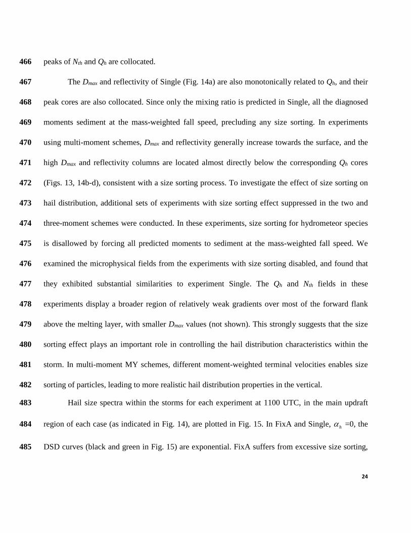
compared with other experiments. 442
3) Hailstone distribution characteristics within storms 443
Given the significant differences in the predicted surface hail size distributions among 444
various MP schemes, we next examine hail distribution properties within simulated storms. 445
23
Microphysical fields, including the hail mass content (Qh), total hail number concentration (Nth), 446
maximum hail size (Dmax), and reflectivity (Z) are examined at 1100 UTC, when the cells are 447
vigorous and well-developed (see Figs. 13 and 14). Vertical cross sections are taken from west to 448
east, passing through the primary hail mass core of the simulated cells; the rough location is 449
indicated by the thick black line in Fig. 2c. Hail size spectra at some typical points in sensitivity 450
experiments are also examined (Fig. 15). 451
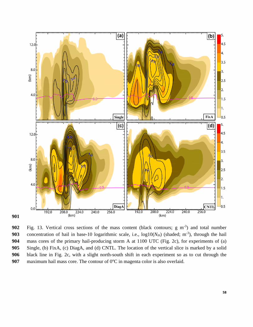
The hail distribution characteristics within the storms from various experiments exhibit large 452
differences (Fig. 13). For example, FixA and DiagA produce copious hail mass aloft, with a peak 453
Qh of 13 g m-3 (Fig. 13b, x ~200-216 km, z ~7-9 km; Fig. 13c, x ~212-217 km, z ~8-10 km), while 454
the peak Qh in CNTL and Single is only about 7 g m-3 (Figs. 13a, d, x ~198-202 km, z ~4-6 km). Nth 455
fields from the two-moment simulations are generally similar to CNTL, all have larger Nth values 456
(>103 m-3) in the storm anvil region above the freezing level. The magnitudes of the peak Nth in 457
FixA are one to two orders higher than the peak Nth values in CNTL, especially in the rear part of 458
the cell (Fig. 13b, x ~165-204 km, z ~2-7 km; Fig. 13c, x ~201-208 km, z ~4-6 km). Similar 459
conclusions about the over-prediction of Qh and Nth for two-moment schemes had also been made in 460
Loftus and Cotton (2014b) and MY06b in their hailstorm simulations. The over-prediction of the 461
moments for the two-moment scheme with a fixed shape parameter could be ascribed to the 462
excessive size sorting and inability to narrow the particle size spectrum with time (Milbrandt and 463
McTaggart-Cowan 2010). Nth diagnosed by Single is considerably different from the other runs; the 464
peak in Nth is much smaller (<102.5 m-3). Since Nth in Single is a monotonic function of Qh, the 465
24
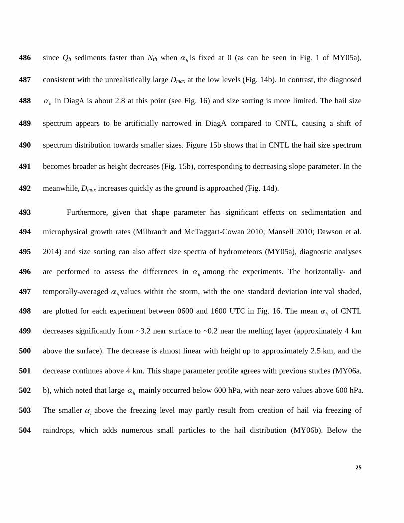
peaks of Nth and Qh are collocated. 466
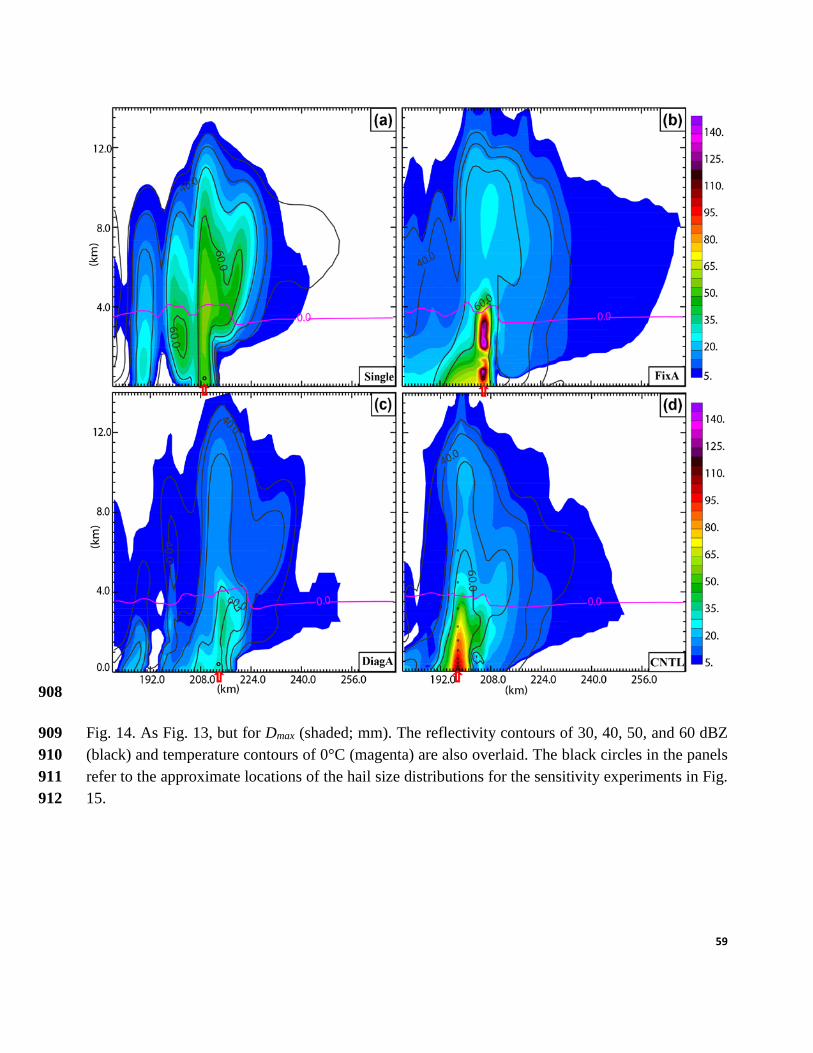
The Dmax and reflectivity of Single (Fig. 14a) are also monotonically related to Qh, and their 467
peak cores are also collocated. Since only the mixing ratio is predicted in Single, all the diagnosed 468
moments sediment at the mass-weighted fall speed, precluding any size sorting. In experiments 469
using multi-moment schemes, Dmax and reflectivity generally increase towards the surface, and the 470
high Dmax and reflectivity columns are located almost directly below the corresponding Qh cores 471
(Figs. 13, 14b-d), consistent with a size sorting process. To investigate the effect of size sorting on 472
hail distribution, additional sets of experiments with size sorting effect suppressed in the two and 473
three-moment schemes were conducted. In these experiments, size sorting for hydrometeor species 474
is disallowed by forcing all predicted moments to sediment at the mass-weighted fall speed. We 475
examined the microphysical fields from the experiments with size sorting disabled, and found that 476
they exhibited substantial similarities to experiment Single. The Qh and Nth fields in these 477
experiments display a broader region of relatively weak gradients over most of the forward flank 478
above the melting layer, with smaller Dmax values (not shown). This strongly suggests that the size 479
sorting effect plays an important role in controlling the hail distribution characteristics within the 480
storm. In multi-moment MY schemes, different moment-weighted terminal velocities enables size 481
sorting of particles, leading to more realistic hail distribution properties in the vertical. 482
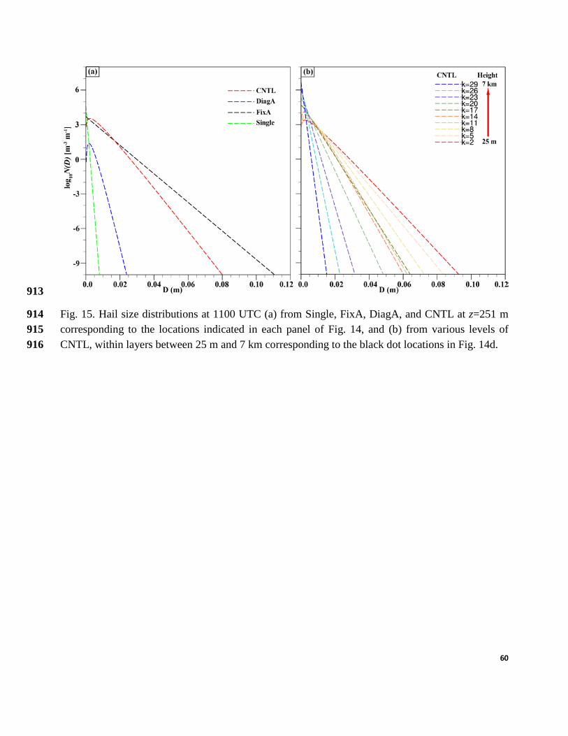
Hail size spectra within the storms for each experiment at 1100 UTC, in the main updraft 483
region of each case (as indicated in Fig. 14), are plotted in Fig. 15. In FixA and Single, hα =0, the 484
DSD curves (black and green in Fig. 15) are exponential. FixA suffers from excessive size sorting, 485
25
since Qh sediments faster than Nth when hα is fixed at 0 (as can be seen in Fig. 1 of MY05a), 486
consistent with the unrealistically large Dmax at the low levels (Fig. 14b). In contrast, the diagnosed 487
hα in DiagA is about 2.8 at this point (see Fig. 16) and size sorting is more limited. The hail size 488
spectrum appears to be artificially narrowed in DiagA compared to CNTL, causing a shift of 489
spectrum distribution towards smaller sizes. Figure 15b shows that in CNTL the hail size spectrum 490
becomes broader as height decreases (Fig. 15b), corresponding to decreasing slope parameter. In the 491
meanwhile, Dmax increases quickly as the ground is approached (Fig. 14d). 492
Furthermore, given that shape parameter has significant effects on sedimentation and 493
microphysical growth rates (Milbrandt and McTaggart-Cowan 2010; Mansell 2010; Dawson et al. 494
2014) and size sorting can also affect size spectra of hydrometeors (MY05a), diagnostic analyses 495
are performed to assess the differences in hα among the experiments. The horizontally- and 496
temporally-averaged hα values within the storm, with the one standard deviation interval shaded, 497
are plotted for each experiment between 0600 and 1600 UTC in Fig. 16. The mean hα of CNTL 498
decreases significantly from ~3.2 near surface to ~0.2 near the melting layer (approximately 4 km 499
above the surface). The decrease is almost linear with height up to approximately 2.5 km, and the 500
decrease continues above 4 km. This shape parameter profile agrees with previous studies (MY06a, 501
b), which noted that large hα mainly occurred below 600 hPa, with near-zero values above 600 hPa. 502
The smaller hα above the freezing level may partly result from creation of hail via freezing of 503
raindrops, which adds numerous small particles to the hail distribution (MY06b). Below the 504
26
freezing level, smaller hail particles tend to melt quickly, increasing hα . In any case, the hα profile 505
of CNTL indicates its variation with height from 0 to 5, suggesting that using a fixed hα value is 506
inappropriate. 507
Although the diagnosed hα in DiagA exhibits a vertical profile with right trend, it differs 508
quite significantly from that of CNTL. The diagnosed hα does not decrease quickly with height and 509
maintains high values (around 2.9) at upper levels (Fig. 16). These result directly from the hα 510
diagnostic formula used (see Eq. 12 in MY05a) that keeps the diagnosed value within a range of 2.8 511
to 4.5 for Dmh below 8 mm. This diagnostic relation was obtained using a one-dimensional model 512
where only the sedimentation process was considered (MY05b); it appears to be inaccurate 513
compared to values produced by the three-moment scheme. 514
c. Microphysical budget analyses 515
To gain additional physical insights regarding the differences between MP schemes, budget 516
analyses of microphysical processes within the simulated storms are performed. The hail production 517
terms are integrated over the entire 1-km simulation domain from surface to model top, according to 518
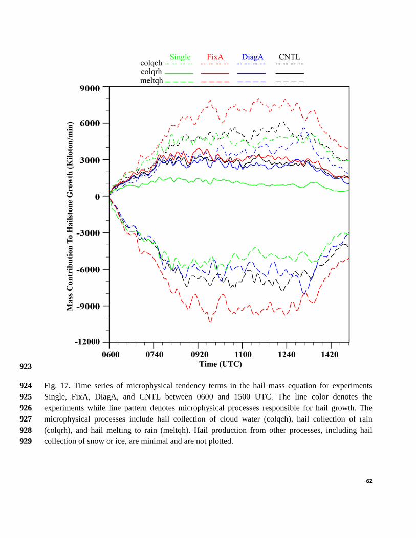
hail mixing ratio prediction equation for the MY scheme (see Eq. [A7] in MY05b). Figure 17 shows 519
the time series of total hail production tendency terms, including hail collection of rain (colqrh) and 520
cloud water (colqch), and hail melting to rain (meltqh), for the four experiments. Other processes, 521
including hail collection of snow or ice, are minimal (Heymsfield and Pflaum 1985), and are not 522
shown. Terms colqrh, colqch and meltqh in FixA are significantly larger than those in other 523
experiments between 0600 and 1500 UTC, with peak rates of approximate 3000, 8000 and -10200 524
27
kiloton/min at 0930 UTC, respectively. In other experiments, hail growth rates from these processes 525
are smaller, especially in DiagA and Single. Generally speaking, the main differences in hail growth 526
processes among the experiments match the differences in the predicted hail mass distributions 527
within storms and hail accumulation at surface, as discussed earlier. 528
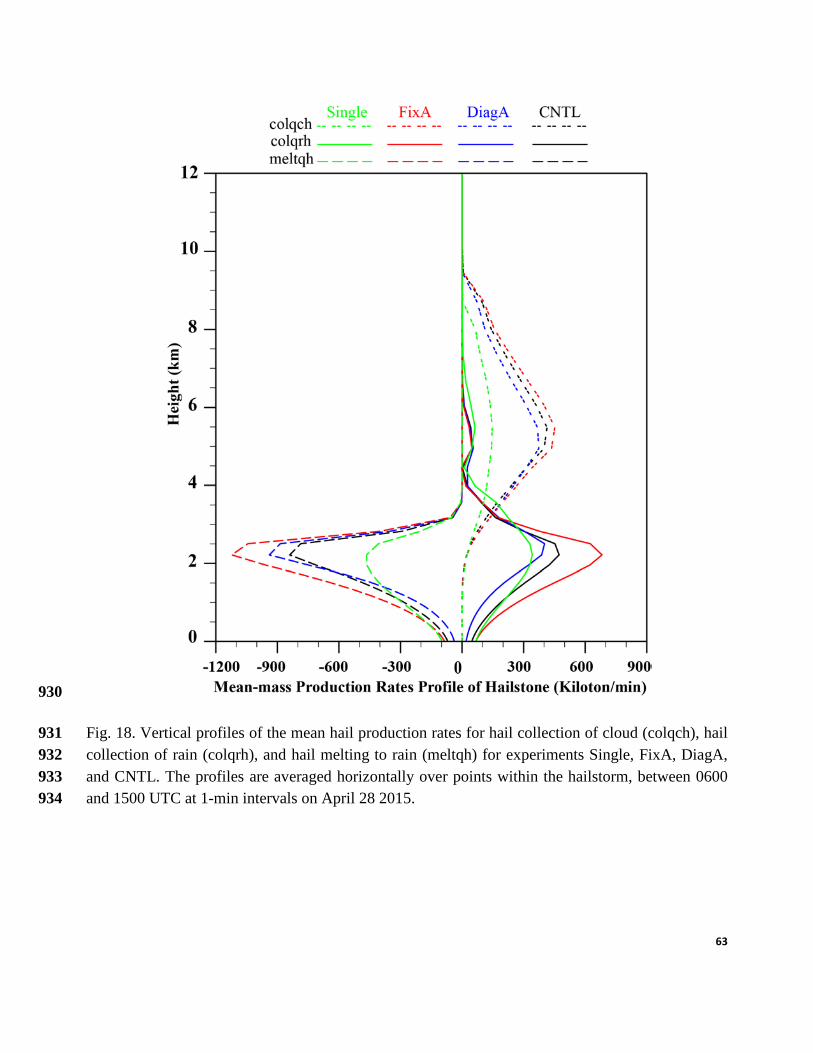
Time-averaged vertical profiles of hail production terms colqrh, colqch and meltqh are 529
plotted in Fig. 18. The profiles are averaged horizontally over points within the hailstorm during its 530
lifespan between 0600 and 1500 UTC with data at 1-minute intervals. The profiles exhibit generally 531
similar vertical patterns for the four experiments, with larger values of colqrh and meltqh occurring 532
below ~4 km (around the height of freezing level), and colqch within the layer between ~2.5 and ~9 533
km. For experiments using multi-moment MP schemes, substantial differences are mainly located 534
below the melting layer. Compared to the peaks values of CNTL (485 kiloton/min for colqrh and -535
840 kiloton/min for meltqh), FixA has much larger peak values of colqrh (696 kiloton/min) and 536
meltqh (-1212 kiloton/min). These larger peak values appear to reflect rapid growth of larger 537
hailstones in FixA through colqrh below the melting layer; the sensible heating from colqrh is offset 538
by the cooling of rapid melting of copious amounts of smaller hail, which may lead to more 539
excessive size sorting. In DiagA, as the hail size spectrum is artificially narrowed (see Fig. 15a), 540
lower collection efficiency of smaller hailstones leads to smaller peak colqrh (396 kiloton/min). The 541
smaller hailstones tend to melt more quickly (-922 kiloton/min), and have lower terminal velocities; 542
these effects combine to result in fewer hailstones accumulating at the surface (see Figs. 11c, 12c). 543
6. Summary and conclusions 544
28
This study evaluates the ability of different MP schemes within storm-scale NWP model 545
runs at a 1-km grid spacing to explicitly predict hail in a long-lasting multi-cellular hailstorm that 546
occurred in Jiangsu Province, China on 28 April, 2015. The hailstorm started within a strong low-547
level convergence between two low-level cyclones that are underneath an upper-level cut-off low 548
within a deep coastal trough. The environment, associated with a weak warm-moist PBL-capping 549
inversion, featured strong 0-6 km wind shear, moderate CAPE, and a very low CIN. The mid-levels 550
were relatively dry. Such an environment is generally conducive to deep convection that tends to 551
produce large hailstones. 552
The simulations employed one-, two-, and three-moment MY MP schemes (MY05a, 05b). 553
Two variants of two-moment schemes were used, one in which the shape parameters of 554
hydrometeors were fixed at zero, and the other in which the shape parameters were diagnosed as a 555
monotonically increasing function of the mean mass-weighted diameter of hydrometeor particles. 556
Evaluations were performed against available observations, including radar reflectivity, radar-557
derived maximum estimated hail size (MESH), and available severe weather reports. Furthermore, 558
neighborhood-based fraction skill scores (FSSs) were calculated for the simulated MESH fields for 559
objective evaluation. 560
Evaluations against observed radar reflectivity indicate that the time and location of the 561
hailstorm initiation and the later organization of storm cells into a large bow-echo are reasonably 562
reproduced by all experiments. Compared with radar observations, experiment FixA, which uses a 563
fixed shape parameter of zero, substantially over-predicts the magnitudes of reflectivity, and as a 564
29
result produces unrealistically high MESH values (with maxima exceeding 70 mm) compared with 565
radar-derived MESH (which has maxima of only 40-50 mm). In contrast, in Single and DiagA that 566
uses a single-moment and diagnostic shape parameter scheme, respectively, reflectivity and MESH 567
fields are under-predicted in both intensity and extent. CNTL using three-moment MY scheme 568
produces MESH swaths that agree more closely with radar-derived MESH swaths than other 569
experiments, and neighborhood-based MESH evaluations further show that the three-moment 570
scheme has notably higher fractional skill scores at all spatial scales compared to the other schemes, 571
especially for large hailstones. 572
Surface accumulated hail mass, number, and hail distribution characteristics within storms 573
are inter-compared among the experiments. Results suggest that FixA produces significant amounts 574
of large hail accumulated over a much wider swath than CNTL. For Single and DiagA, the peak 575
SAHNC values are about two orders of magnitude smaller than those of CNTL, especially in DiagA 576
where almost no hail larger than 40 mm is produced. Examinations of hail distributions within 577
storms indicate that since all the moments of a given hydrometeor type are monotonically related to 578
the mixing ratio (which is the only moment predicted) in Single, no size sorting can occur. For 579
multi-moment schemes, different moment-weighted terminal velocities allow for size sorting of 580
particles, making it possible to reproduce more realistic PSDs within the storm. However, 581
substantial differences in the hail size distributions are still present within storms simulated using 582
different multi-moment schemes. For example, FixA, which uses a two-moment scheme with a 583
fixed xα value of zero, suffers from excessive size sorting which leads to an unrealistic shift in hail 584
30
DSD towards larger hailstones during sedimentation. On the other hand, the diagnostic xα used in 585
DiagA is at least 2.8, resulting in a hail size spectrum that appears to be artificially narrowed 586
compared to CNTL; it causes a spectrum shift towards smaller hailstones and yields smaller Dmax 587
and SAHNC. These results indicate that although excessive size sorting is more limited in DiagA, 588
the specific xα diagnostic relation derived from sedimentation-only one-dimensional model appears 589
inaccurate. Therefore, more accurate diagnostic relations for xα may need to be derived, using 590
perhaps output from full three-moment simulations. In fact, our preliminary results using this 591
approach are encouraging and more complete results will be reported in a separate paper. 592
Furthermore, budget analyses of hail production terms suggest that collection of rain and 593
cloud water by hail are dominant contributors to hail mass growth. The differences in hail growth 594
processes among different experiments are closely linked to the treatment of shape parameter in 595
different MP schemes, which further lead to the differences in the predicted surface accumulated 596
hail mass, SAHNC, and hail distribution within the simulated storms. 597
In the end, we note that there are many other possible configurations for one- or two-598
moment MP schemes in terms of the choice of fixed or variable intercept and shape parameters, 599
which can be further evaluated in the future. We also note that due to the lack of reliable 600
observations of surface accumulated hailstones, evaluations of explicit hail prediction in this paper 601
carries a certain degree of uncertainty. In-situ observations of microphysical processes, as well as 602
hail size distributions are needed for more reliable evaluations. 603
604
31
Acknowledgement. This work was primarily supported by the National 973 Fundamental Research 605
Program of China (2013CB430103). Liping Luo was supported by Nanjing University for her 606
extended visit at CAPS, University of Oklahoma. The work was also supported by the National 607
Science Foundation of China (Grant No. 41405100), Foundation of China Meteorological 608
Administration special (Grant No. GYHY201506006). We gratefully acknowledge the High 609
Performance Center (HPCC) of Nanjing University for doing the numerical calculations in this 610
paper on its IBM Blade cluster system. The second author acknowledges the support of the National 611
Thousand Person Plan hosted at the Nanjing University, and the support of NSF grants AGS-612
1261776 for the Severe Hail, Analysis, Representation, and Prediction (SHARP) project. Nathan 613
Snook and Jonathan Labriola are thanked for proofreading and improving the manuscript. 614
Suggestions and comments from three anonymous reviewers also improved our paper. The NCEP 615
FNL analysis data can be downloaded freely at http://rda.ucar.edu/datasets/ds083.2/ The radar 616
dataset is provided by the Climate Data Center at National Meteorological Information Center of 617
China Meteorological Administration, and processed data used in this paper are available at 618
6 4 5 4 4 40 0 03 10 , 4 10 , 4 10s g hN m N m N m− − −= × = × = ×
764
765
41
List of figures 766
Fig. 1. Twenty-four-hour reports of severe weather in eastern China, starting from 2715 UTC 28 767
April 2015. Provinces of Shandong and Jiangsu are labeled in red. The open black circles 768
indicate the locations of six operational S-band radars at Jinan, Xuzhou, Bengbu, Yancheng, 769
Nanjing, and Nantong. The large gray dashed circles denote the 230-km range ring for each 770
radar. The red “×” denotes the location of the extracted sounding shown in Fig. 4. The base 771
map is obtained from Severe Weather Report Maps of Chinese Meteorological Society. 772
Fig. 2. Composite (column-maximum) reflectivity fields of operational radars from 0900 to 1400 773
UTC at 1-h interval. Provinces of Shandong, Jiangsu, and Anhui are labeled in black. The 774
thick straight line in (c) marks the rough location of vertical cross sections presented in Fig. 775
13 and 14. 776
Fig. 3. Synoptic features of (a) 200 hPa, (b) 500 hPa, (c) 850 hPa, and (d) 1000 hPa at 0600 UTC 28 777
April 2015, showing wind barbs (one full barb denotes 2.5 m s-1), temperature (magenta 778
dashed contours, with interval of 4oC), geopotential height (solid black contours, gpm). The 779
shadings in (a) and (b) denote the horizontal wind speed (m s-1), and that in (d) denotes 780
convective available energy (J kg-1). The bold solid brown lines in (a) and (b), (c) and (d) 781
indicate trough lines and shear lines, respectively. Jiangsu Province is outlined by red solid 782
42
line in (a), and the blue capital C denotes the COLs at 500 hPa and cyclonic circulations at 783
850 and 1000 hPa. The maps are drawn from NCEP GFS final analysis (FNL) data. 784
Fig. 4. Skew-T plot of a sounding extracted from NCEP FNL analysis data at (34oN, 117oE) at 0600 785
UTC 28 April 2015 near Xuzhou. 786
Fig. 5. Model domains of 3 km (outer black box) and 1 km (inner red box) grid spacings for the 787
hailstorm simulations. Terrain elevation (m) is plotted in color. Cities of Jinan, Changzhou, 788
Wuxi, and Suzhou where hailstones are reported are labeled in black. The city of Yizheng is 789
labeled in magenta, where maximum hail size is registered of around 10 cm. Provinces of 790
Shandong, Jiangsu, and Anhui are labeled in red. 791
Fig. 6. Composite (column-maximum) reflectivity fields from simulations using different 792
microphysics schemes and operational radar observations, namely (a) Single, (b) FixA, (c) 793
DiagA, (d) CNTL, and (e) radar observations at 0900 UTC 28 April 2015. 794
Fig. 7. As Fig. 6, but at 1400 UTC 28 April 2015. 795
Fig. 8. Simulated MESH with one-, two- and three-moment microphysics schemes, namely (a) 796
Single, (b) FixA, (c) DiagA, (d) CNTL, and (e) observed MESH derived from WSR-98D 797
radar observations. The MESH fields are created as a composite from observed/simulated 798
data between 0600 and 1600 UTC at 5-minute intervals. Locations of the cities of 799
Changzhou, Wuxi, and Suzhou, where hail was reported are represented by the black “×”. 800
43
The city of Yizheng is labeled in magenta, where maximum hail size is registered of around 801
10 cm. 802
Fig. 9. Fraction skill scores of MESH from 0600 to 1600 UTC for the experiments, i.e., Single, 803
FixA, DiagA, and CNTL, with MESH exceeding (a) 30 mm and (b) 40 mm, over 804
neighborhood radii of 10, 30, 50, and 60 km. FSSuseful value is also shown. 805
Fig. 10. Surface accumulated solid precipitation in water-equivalent depth (mm) between 0600 and 806
1600 UTC from simulations (a) Single, (b) FixA, (c) DiagA, and (d) CNTL. 807
Fig. 11. Surface accumulated hail number concentration (SAHNC) between 0600 and 1600 UTC at 808
60-second intervals on 28 April 2015, derived from simulations (a) Single, (b) FixA, (c) 809
DiagA, and (d) CNTL, with hail diameter larger than 30 mm. SAHNC is in base-10 810
logarithmic scale, i.e., log10(SAHNC) (m-2). 811
Fig. 12. As Fig. 11, but for hail diameter exceeding 40 mm. 812
Fig. 13. Vertical cross sections of the mass content (black contours; g m-3) and total number 813
concentration of hail in base-10 logarithmic scale, i.e., log10(Nth) (shaded; m-3), through the 814
hail mass cores of the primary hail-producing storm A at 1100 UTC (Fig. 2c), for 815
experiments of (a) Single, (b) FixA, (c) DiagA, and (d) CNTL. The location of the vertical 816
slice is marked by a solid black line in Fig. 2c, with a slight north-south shift in each 817
experiment so as to cut through the maximum hail mass core. The contour of 0oC in magenta 818
color is also overlaid. 819
44
Fig. 14. As Fig. 13, but for Dmax (shaded; mm). The reflectivity contours of 30, 40, 50, and 60 dBZ 820
(black) and temperature contours of 0°C (magenta) are also overlaid. The black circles in the 821
panels refer to the approximate locations of the hail size distributions for the sensitivity 822
experiments in Fig. 15. 823
Fig. 15. Hail size distributions at 1100 UTC (a) from Single, FixA, DiagA, and CNTL at z=251 m 824
corresponding to the locations indicated in each panel of Fig. 14, and (b) from various levels 825
of CNTL, within layers between 25 m and 7 km corresponding to the black dot locations in 826
Fig. 14d. 827
Fig. 16. Profiles of the shape parameters of experiments of Single, FixA, DiagA, and CNTL. The 828
profiles are horizontal averages within the simulated hailstorms over the 1-km domain of the 829
simulations between 0600 and 1600 UTC at 1-min interval. The shaded areas denote the one 830
standard deviation from the average profiles. 831
Fig. 17. Time series of microphysical tendency terms in the hail mass equation for experiments 832
Single, FixA, DiagA, and CNTL, between 0600 and 1500. The line color denotes the 833
experiments while line pattern denotes microphysical processes responsible for hail growth. 834
The microphysical processes include hail collection of cloud water (colqch), hail collection 835
of rain (colqrh), and hail melting to rain (meltqh). Hail production from other processes, 836
including hail collection of snow or ice, are minimal and are not plotted. 837
45
Fig. 18. Vertical profiles of the mean hail production rates for hail collection of cloud (colqch), hail 838
collection of rain (colqrh), and hail melting to rain (meltqh) for experiments Single, FixA, 839
DiagA, and CNTL. The profiles are averaged horizontally over points within the hailstorm 840
between 0600 and 1500 UTC at 1-min intervals on April 28 2015. 841
842
46
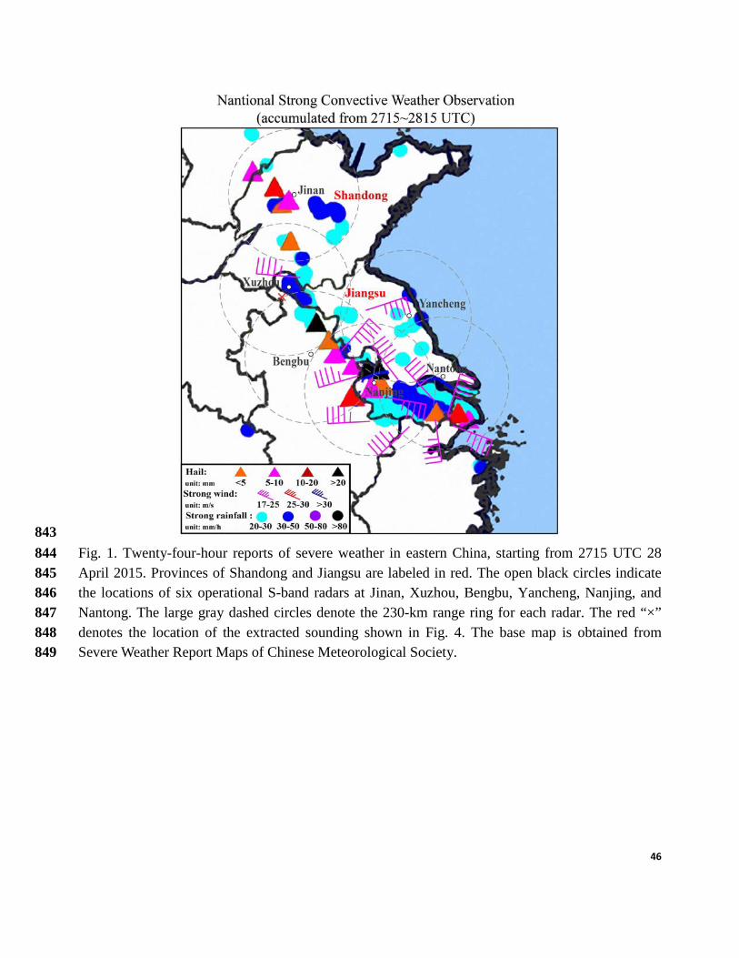
843 Fig. 1. Twenty-four-hour reports of severe weather in eastern China, starting from 2715 UTC 28 844 April 2015. Provinces of Shandong and Jiangsu are labeled in red. The open black circles indicate 845 the locations of six operational S-band radars at Jinan, Xuzhou, Bengbu, Yancheng, Nanjing, and 846 Nantong. The large gray dashed circles denote the 230-km range ring for each radar. The red “×” 847 denotes the location of the extracted sounding shown in Fig. 4. The base map is obtained from 848 Severe Weather Report Maps of Chinese Meteorological Society. 849
47
850
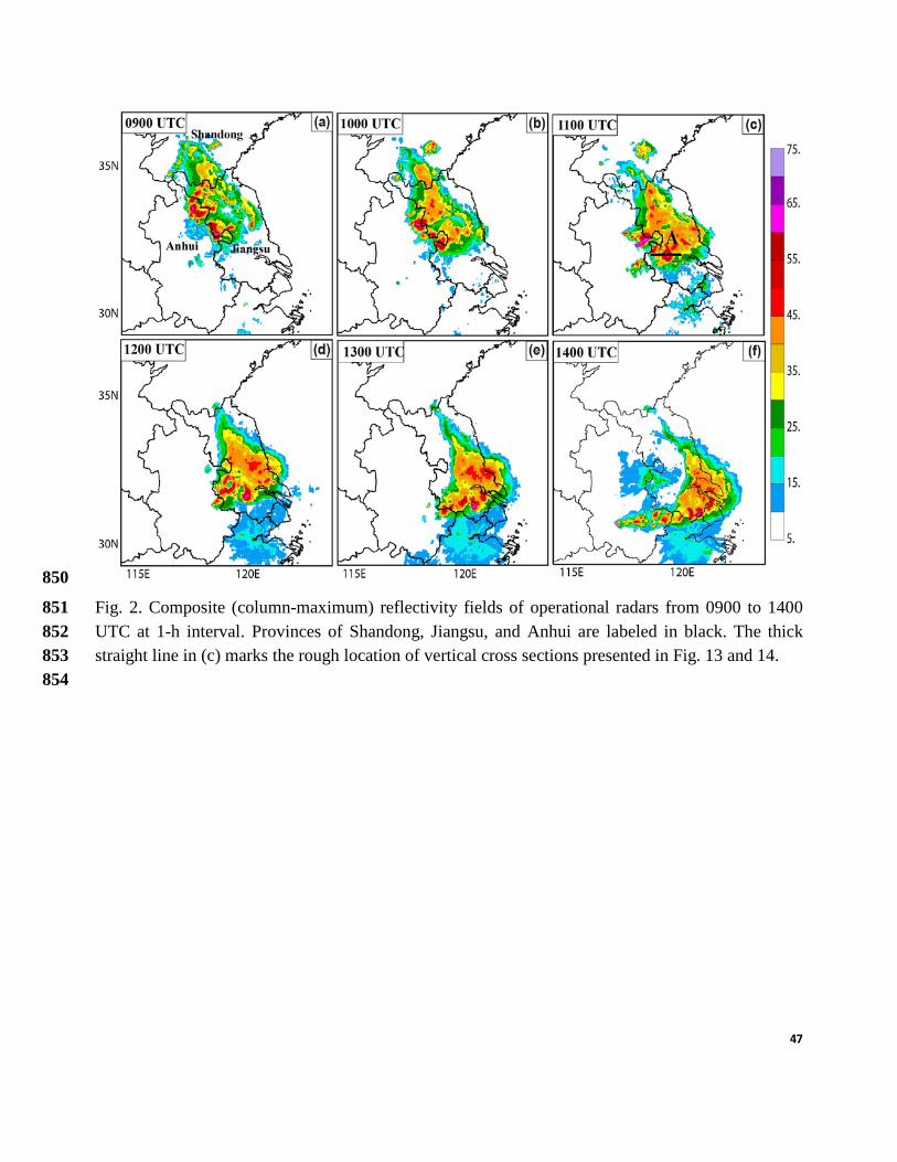
Fig. 2. Composite (column-maximum) reflectivity fields of operational radars from 0900 to 1400 851 UTC at 1-h interval. Provinces of Shandong, Jiangsu, and Anhui are labeled in black. The thick 852 straight line in (c) marks the rough location of vertical cross sections presented in Fig. 13 and 14. 853 854
48
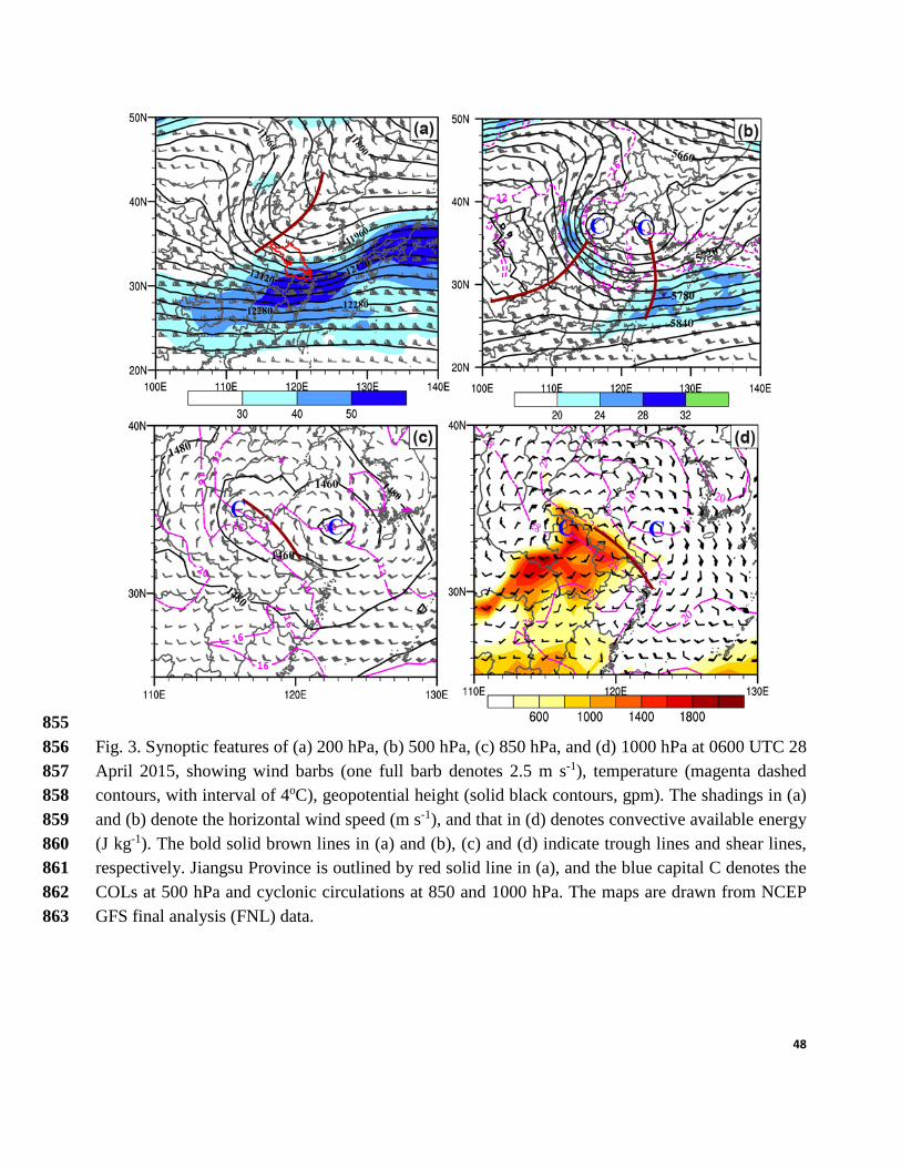
855 Fig. 3. Synoptic features of (a) 200 hPa, (b) 500 hPa, (c) 850 hPa, and (d) 1000 hPa at 0600 UTC 28 856 April 2015, showing wind barbs (one full barb denotes 2.5 m s-1), temperature (magenta dashed 857 contours, with interval of 4oC), geopotential height (solid black contours, gpm). The shadings in (a) 858 and (b) denote the horizontal wind speed (m s-1), and that in (d) denotes convective available energy 859 (J kg-1). The bold solid brown lines in (a) and (b), (c) and (d) indicate trough lines and shear lines, 860 respectively. Jiangsu Province is outlined by red solid line in (a), and the blue capital C denotes the 861 COLs at 500 hPa and cyclonic circulations at 850 and 1000 hPa. The maps are drawn from NCEP 862 GFS final analysis (FNL) data. 863
49
864
Fig. 4. Skew-T plot of a sounding extracted from NCEP FNL analysis data at (34oN, 117oE) at 0600 865 UTC 28 April 2015 near Xuzhou. 866
50
867
Fig. 5. Model domains of 3 km (outer black box) and 1 km (inner red box) grid spacings for the 868 hailstorm simulations. Terrain elevation (m) is plotted in color. Cities of Jinan, Changzhou, Wuxi, 869 and Suzhou where hailstones are reported are labeled in black. The city of Yizheng is labeled in 870 magenta, where maximum hail size is registered of around 10 cm. Provinces of Shandong, Jiangsu, 871 and Anhui are labeled in red. 872
51
873
Fig. 6. Composite (column-maximum) reflectivity fields from simulations using different 874 microphysics schemes and operational radar observations, namely (a) Single, (b) FixA, (c) DiagA, 875 (d) CNTL, and (e) radar observations at 0900 UTC 28 April 2015. 876
52
877
Fig. 7. As Fig. 6, but at 1400 UTC 28 April 2015. 878
53
879 Fig. 8. Simulated MESH with one-, two- and three-moment microphysics schemes, namely (a) 880
54
Single, (b) FixA, (c) DiagA, (d) CNTL, and (e) observed MESH derived from WSR-98D radar 881 observations. The MESH fields are created as a composite from observed/simulated data between 882 0600 and 1600 UTC at 5-minute intervals. Locations of the cities of Changzhou, Wuxi, and Suzhou, 883 where hail was reported are represented by the black “×”. The city of Yizheng is labeled in magenta, 884 where maximum hail size is registered of around 10 cm. 885 886
887
Fig. 9. Fraction skill scores of MESH from 0600 to 1600 UTC for the experiments, i.e., Single, 888 FixA, DiagA, and CNTL, with MESH exceeding (a) 30 mm and (b) 40 mm, over neighborhood 889 radii of 10, 30, 50, and 60 km. FSSuseful value is also shown. 890
55
891
Fig. 10. Surface accumulated solid precipitation in water-equivalent depth (mm) between 0600 and 892 1600 UTC from simulations (a) Single, (b) FixA, (c) DiagA, and (d) CNTL. 893
56
894
Fig. 11. Surface accumulated hail number concentration (SAHNC) between 0600 and 1600 UTC at 895 60-second intervals on 28 April 2015, derived from simulations (a) Single, (b) FixA, (c) DiagA, and 896 (d) CNTL, with hail diameter larger than 30 mm. SAHNC is in base-10 logarithmic scale, i.e., 897 log10(SAHNC) (m-2). 898
57
899
Fig. 12. As Fig. 11, but for hail diameter exceeding 40 mm. 900
58
901
Fig. 13. Vertical cross sections of the mass content (black contours; g m-3) and total number 902 concentration of hail in base-10 logarithmic scale, i.e., log10(Nth) (shaded; m-3), through the hail 903 mass cores of the primary hail-producing storm A at 1100 UTC (Fig. 2c), for experiments of (a) 904 Single, (b) FixA, (c) DiagA, and (d) CNTL. The location of the vertical slice is marked by a solid 905 black line in Fig. 2c, with a slight north-south shift in each experiment so as to cut through the 906 maximum hail mass core. The contour of 0oC in magenta color is also overlaid. 907
59
908
Fig. 14. As Fig. 13, but for Dmax (shaded; mm). The reflectivity contours of 30, 40, 50, and 60 dBZ 909 (black) and temperature contours of 0°C (magenta) are also overlaid. The black circles in the panels 910 refer to the approximate locations of the hail size distributions for the sensitivity experiments in Fig. 911 15. 912
60
913
Fig. 15. Hail size distributions at 1100 UTC (a) from Single, FixA, DiagA, and CNTL at z=251 m 914 corresponding to the locations indicated in each panel of Fig. 14, and (b) from various levels of 915 CNTL, within layers between 25 m and 7 km corresponding to the black dot locations in Fig. 14d. 916
61
917
Fig. 16. Profiles of the shape parameters of experiments of Single, FixA, DiagA, and CNTL. The 918 profiles are horizontal averages within the simulated hailstorms over the 1-km domain of the 919 simulations between 0600 and 1600 UTC at 1-min interval. The shaded areas denote the one 920 standard deviation from the average profiles. 921
922
62
923
Fig. 17. Time series of microphysical tendency terms in the hail mass equation for experiments 924 Single, FixA, DiagA, and CNTL between 0600 and 1500 UTC. The line color denotes the 925 experiments while line pattern denotes microphysical processes responsible for hail growth. The 926 microphysical processes include hail collection of cloud water (colqch), hail collection of rain 927 (colqrh), and hail melting to rain (meltqh). Hail production from other processes, including hail 928 collection of snow or ice, are minimal and are not plotted. 929
63
930
Fig. 18. Vertical profiles of the mean hail production rates for hail collection of cloud (colqch), hail 931 collection of rain (colqrh), and hail melting to rain (meltqh) for experiments Single, FixA, DiagA, 932 and CNTL. The profiles are averaged horizontally over points within the hailstorm, between 0600 933 and 1500 UTC at 1-min intervals on April 28 2015. 934